MAGAN: Margin Adaptation for GenerativeAdversarial Networks

Ruohan Wang Antoine Cully∗ Hyung Jin Chang∗ Yiannis DemirisPersonal Robotics Laboratory, Department of Electrical and Electronic Engineering

Imperial College London, United Kingdom{r.wang16, a.cully, hj.chang, y.demiris}@imperial.ac.uk

Abstract

We propose the Margin Adaptation for Generative Adversarial Networks (MA-GANs) algorithm, a novel training procedure for GANs to improve stability andperformance by using an adaptive hinge loss function. We estimate the appropriatehinge loss margin with the expected energy of the target distribution, and deriveprincipled criteria for when to update the margin. We prove that our method con-verges to its global optimum under certain assumptions. Evaluated on the task ofunsupervised image generation, the proposed training procedure is simple yet ro-bust on a diverse set of data, and achieves qualitative and quantitative improvementscompared to the state-of-the-art.

1 Introduction

Generative Adversarial Networks (GANs) [1] are generative models known for their ability to samplefrom complex and intractable distributions, inherent in tasks such as realistic image generation fromnatural scenes. GANs are designed as a competitive game between the generator and discrimina-tor network, whereby the generator tries to fool the discriminator with synthetic data, while thediscriminator tries to differentiate the real data from the synthetic one. At its theoretical optimum,the generator produces samples indistinguishable from the real data. GANs have been applied tomany interesting areas, including image super-resolution [2], driving behavior modeling [3], and dataaugmentation [4].

Training GANs remains a challenge. The quality of generated samples for complex distributionssuch as natural scenes is unsatisfactory, as they often contain visible artifacts and unrecognizablestructures. In addition, GANs suffer from potential mode collapse whereby the generator onlyproduces similar images [5], and a lack of convergence measures [6]. Recent techniques includingbatch discrimination [7] and Wasserstein distance loss [6] have addressed the above problems tovarying degrees of success. However, they often introduce additional complexity such as weightclipping and new hyper-parameters, which demands significant tuning to achieve the best result.

Energy-based GANs (EBGANs) [8] use an auto-encoder as the discriminator, and define the energyof each sample as its reconstruction loss computed by the auto-encoder. The auto-encoder aimsto assign lower energy to the real data than the synthetic one. EBGANs introduce a hinge lossobjective function aimed at stabilizing the training, so that the discriminator could ignore syntheticsamples with high energy. Finding an appropriate margin value is crucial for successful training andis dependent on both architecture choice and data complexity [8].

In this paper, we propose Margin Adaptation for Generative Adversarial Networks (MAGANs),that automatically adapts the margin using the expected energy of the real data distribution, whichimproves the training stability by maintaining the equilibrium between the discriminator and thegenerator.

∗These authors contributed equally to this work

arX

iv:1

704.

0381

7v3

[cs

.LG

] 2

3 M

ay 2

017

The main contributions of this paper are:

• A simple and robust training procedure for auto-encoder based GANs that adapts the hinge lossmargin based on training statistics. This approach does not introduce any new hyper-parametersand removes the dependence on the margin hyper-parameter introduced by EBGANs.

• We prove that both EBGANs and MAGANs converge to their global optima under certain assump-tions, and that MAGANs converge under more relaxed ones.

• A set of experiments that demonstrate the robustness and stability of our approach in producingvisually appealing samples with relatively simple network architectures, and improvements overthe state-of-the-art results on a diverse set of datasets.

2 Related Work

Generative Adversarial Networks (GANs) [1] are a class of generative sampling methods for modelingintractable distributions. Primary challenges of training GANs are summarized and discussedin [5]. Among them, the difficulty in maintaining the equilibrium between the discriminator andgenerator often lead to training instability, as one network overpowers the other. Furthermore, visualinspection of generated samples is typically the only practical method to estimate convergence as thevalue of loss function fluctuates [5, 6]. Various techniques have been proposed to improve GANstraining [7, 9] to varying degrees of success. Notably, Wasserstein GANs (WGANs) [6] provided thefirst convergence measure in GANs training using a loss function based on Wasserstein distance. Tocompute the Wasserstein distance, the discriminator uses weight clipping, which significantly limitsthe network capacity. Weight clipping has been later replaced with a gradient norm constraint in [10].Unfortunately, these advances often introduce additional hyper-parameters, requiring significanttuning to achieve best results.

Auto-encoders [11] are extensively used in GANs. In [9], the authors propose an auxiliary lossfunction to match latent features of real and synthetic samples, computed from an auto-encoder. InPlug-and-Play Generative Networks [12], auto-encoders are used for computing the gradient of thelog probability of real data to guide the sampling process. Energy-based GANs (EBGANs) [8] use anauto-encoder for the discriminator, which associates to each sample an energy value using the per-coordinate squared loss. Low energy samples are attributed to samples from the real data manifold,while high energy values are assigned to synthetic samples. EBGANs have been shown to minimizethe total variation (TV) distance between the real and synthetic data distributions [6]. EBGANsintroduce a hinge loss objective function to stabilize the training by allowing the discriminator toignore synthetic samples with energy larger than a predefined margin m (see Eq. 2). Most recently,Boundary Equilibrium GANs (BEGANs) [13] extends EBGANs by proposing a loss function thataims to match the energy of synthetic data to a fraction of the energy of real data. BEGANs sharesome similarities with the approach proposed in this paper, as they both monitor the expected energyof real and synthetic data to control training and generate visually pleasing and coherent samples.However, BEGANs formulate a compulsory trade-off between generation diversity and quality, andrequires a more complex training procedure.

3 Proposed Method

3.1 Definition

Given a data sample x ∈ RNx of dimension Nx, a generated sample G(z) : RNz → RNx andz ∈ RNz of dimension Nz generated from a known distribution, such as the normal distribution.Following [8], we define the discriminator D(x) as:

D(x) = ||Dec(Enc(x))− x|| (1)where D(x) is a deep auto-encoder function. The discriminator loss LD and the generator loss LG

are defined as:LD(x, z) = D(x) +max(0,m−D(G(z))) and LG(z) = D(G(z)) (2)

where m > 0 is a predefined hyper-parameter. We define Edata(D(x)) and EG(D(x)), the expectedenergies of the real data distribution and of the synthetic data distribution respectively as:

Edata(D(x)) =

∫x

pdata(x) ·D(x) dx and EG(D(x)) =

∫x

pG(x) ·D(x) dx (3)

2

where pdata, pG denotes the probability that an arbitrary sample x occurs in the real and syntheticdata distributions respectively. In addition, we define two sets S1 = {x : pdata(x) < pG(x)} andS2 = {x : pdata(x) ≥ pG(x)}

3.2 The MAGANs Model

We have observed reliably in our experiments with EGBANs that the real and synthetic data distri-butions diverge (in terms of expected energy) during training, and that the quality of the generatedsamples stops improving visually (see Section 4.3). To overcome the divergence between the twodistributions, we propose to adapt the margin m to the expected energy of real data when we detectthat the stalling of the generator loss. Intuitively, lowering the margin from a to b limits the powerof the discriminator by preventing it from differentiating against synthetic samples with energyb ≤ D(G(z)) ≤ a. This allows the generator to produce new adversarial examples without theirenergy being simultaneously raised by the discriminator. In turn, the discriminator is presented withnew adversarial samples that better matches the expected energy of the real data.

We define when and how to adapt the margin in the two following section, and present the MAGANstraining procedure in Algorithm 1.

Algorithm 1 MAGANs algorithmRequire: α, the learning rate, b, the batch size, N the training set size, Tmax the max number of training

epochs, w, initial discriminator parameters, θ, initial generator parameters1: m0 = 02: for t = 1 to 2 do . Pre-train discriminator3: for j = 1 to bN/bc do4: Sample {xi}bi=1 a batch from the real data5: gw = Ow[ 1b

∑bi=1D(xi)] . zi ignored as m0 = 0

6: w = w + α×Adamax(w, gw)7: end for8: end for9: m1 = E(D(x)), S0

G =∞10: for t = 1 to Tmax do11: Stdata = 0, StG = 0 . Collect statistics into S to compute E12: for j = 1 to bN/bc do13: Sample {xi}bi=1 a batch from the real data . Train the discriminator14: Sample {zi}bi=1 a batch from the prior samples15: gw = Ow[ 1b

∑bi=1(D(xi) +max(0,mt −D(G(zi))))]

16: Stdata = Stdata +∑bi=1D(xi)

17: w = w + α×Adamax(w, gw)18: Sample {zi}bi=1 a batch from the prior samples . Train the generator19: gθ = Oθ[ 1b

∑bi=1D(G(zi))]

20: θ = θ + α×Adamax(θ, gθ)21: StG = StG +

∑bi=1D(G(zi))

22: end for23: if Stdata/N < mt and Stdata < StG and St−1

G ≤ StG then . Update the margin24: mt+1 = Stdata/N25: end if26: end for

3.2.1 When to Adjust the Margin

We reduce the margin m when the following three conditions hold:

Et−1G ≤ Et

G and Etdata < mt and Et

data < EtG (4)

where EtG denotes EG(D(x)) at the end of training epoch t. Et

data is defined similarly forEdata(D(x)). The conditions capture the intuition that the discriminator should firstly attributelower energy to the real data, which provides sufficient amount of samples with low energy thatthe generator could imitate from. To reduce the noise in computing the expected energy, we collectsample energies across each training epoch and compute the average at the end of each epoch.

3

3.2.2 How to Set the Margin

We choose mt = Etx to guide the generator towards the real data distribution. In practice, the

computation of expectation requires almost no additional resources as the expected energies ofmini-batches are needed for the gradient computation. In order to get an initial estimate of the margin,we pre-train the discriminator with an auto-encoder objective for 2 epochs with only real samples(equivalent to setting m = 0) and compute the expected energy of the real data.

The idea of using the expected energy to control training is also independently proposed in BE-GANs [13], where the loss function aims to match Et

G = γEtdata with γ as a hyper-parameter meant

to control the trade-off between diversity and quality. We observe that our method is different inseveral significant ways:

• We show that our method converges to its global optimum where the real and synthetic datadistributions match exactly. In contrast, BEGANs provide no such guarantee.

• Our method does not introduce new hyper-parameters. On the contrary, we remove the dependenceon the margin hyper-parameter from EBGANs.

• Our method has a simpler training procedure, requiring no learning rate decay nor separate learningrates for the two networks.

3.3 Theoretical Analysis of MAGAN

We show that both MAGANs and EBGANs converge to their global optima under certain assumptions,and that MAGANs converge under more relaxed conditions. We follow the same theoretical assump-tions as in [1] for our analysis. Specifically, we assume that at each update step, 1) the discriminatoris allowed to reach its optimum given the generator, 2) that pG is updated to improve its loss function,and that 3) D and G have infinite capacity. We also assume that D∗(x) = 0 if pdata(x) = pG(x),where D∗ denotes the optimal discriminator to a given generator. For the following demonstrations,we hypothesize that the expected energies can be computed at each iteration t.

3.3.1 Convergence of EBGANs

Lemma 3.1. Let D∗ be the optimal discriminator with respect to a given generator, thenEdata(D

∗(x)) ≤ EG(D∗(x)) ≤ m. In particular, Edata(D

∗(x)) = EG(D∗(x)) if and only if

pdata(x) = pG(x) almost everywhere.

Proof. Since D∗ is optimal with respect to G,

D∗(x) =

{m, if pdata(x) < pG(x)

0, if pdata(x) > pG(x)(5)

if pdata(x) = pG(x), D∗(x) is not unique and 0 ≤ D∗(x) ≤ m. Equation 5 is proven in [8, p. 11].Therefore,

Edata(D∗(x))− EG(D

∗(x)) =

∫S1

(pdata(x)− pG(x)) ·D∗(x) dx (6)

= m ·∫S1

(pdata(x)− pG(x)) dx ≤ 0 (7)

EG(D∗(x)) =

∫x

pG(x)D∗(x) dx ≤ m ·

∫x

pG(x) dx = m (8)

Lastly, if pdata(x) = pG(x) ∀x, it is clear that Edata(D∗(x)) = EG(D

∗(x)). On the other hand, ifEdata(D

∗(x)) = EG(D∗(x)), then

Edata(D∗(x))− EG(D

∗(x)) = m ·∫S1

(pdata(x)− pG(x)) dx = 0 (9)

Since pdata(x)− pG(x) is negative for x ∈ S1, the equality only holds if∫S1

dx = 0. This impliesthat pdata(x) = pG(x) almost everywhere1.

1The last step is proven in Lemma 2 of [8, p. 11]

4

Lemma 3.2. Let Gt and D∗t be the generator and its optimal discriminator at update step t ofEBGANs training, then EGt+1(D

∗t (x)) = EGt+1(D

∗t+1(x)),

Proof. By assumption that D∗(x) = 0 if pdata(x) = pG(x), Equation 5 reduces to

D∗(x) =

{m, if pdata(x) < pG(x)

0, if pdata(x) ≥ pG(x)(10)

As D∗t and D∗t+1 do not change S1 or S2 (only updates to G change S1 and S2),

EGt+1(D∗t (x)) = 0 · pG(S2) +m · pG(S1) = EGt+1

(D∗t+1(x))

Proposition 1. If at each update step, the optimal discriminator is reached given the generator, andpG is updated to reduce EG(D(x)), EBGANs converge to pdata(x) = pG(x) almost everywhere.

Proof. The two conditions combined translates to EGt+1(D∗t (x)) < EGt(D

∗t (x)) ∀t. By Lemma

3.2, EGt+1(D∗t (x)) = EGt+1

(D∗t+1(x)). Therefore,

EGt+1(D∗t+1(x)) = EGt+1

(D∗t (x)) < EGt(D∗t (x)) (11)

This implies that the expected energy of synthetic data strictly decreases at each update step.

From [6], we rewrite the loss function of EBGANs in minimax form under optimal discriminators,

minpG

max0≤D(x)≤m

EG(D(x))− Edata(D(x)) (12)

Noting that the following expression is convex with respect to pG2

EG(D∗(x))− Edata(D

∗(x)) =m

2

∫x

|pG(x)− pdata(x)|dx (13)

and that there exists a unique global optimum when the two distributions exactly match [8, 6].Therefore, with sufficiently small update steps of pG, pG converges to the global optimum, whichimplies pdata(x) = pG(x) almost everywhere.

3.3.2 Convergence of MAGANs

Lemma 3.3. In MAGAN, m strictly decreases and m converges to 0 as long pdata and pG do notmatch exactly.

Proof. When mt is updated to Edata(D∗t (x)), we have mt = Edata(D

∗t (x)) = mt−1 · pdata(S1)

(according to equation 10). Therefore, m strictly decreases and converges to 0, as pdata(S1) < 1.

Proposition 2. If at each update step, the optimal discriminator is reached given the generator, andpG is updated along the direction of −∂EG(D∗(x))

∂pG(x) , MAGANs converge to pdata(x) = pG(x) almosteverywhere.

Proof. We first note that updating pG along the direction of −∂EG(D∗(x))∂pG(x) corresponds to a gradient

descent step of G towards reducing the generator loss function. We do not assume that the updatesteps reduce EG(D(x)) at each step, but only that the directions of the update steps is appropriatewith respect to pG.

We split the proof into two cases: 1) As long as the update steps are small enough such thatEG(D(x)) is reduced after each step, the margin remains unchanged and MAGANs converge to itsglobal optimum (similarly to Proposition 1).

2) If EG(D(x)) increases after a step t because of a too large step, the margin update conditionEGt+1

(D∗t (x)) ≥ EGt(D∗t (x)) is met, and the other two conditions are satisfied by Lemma 3.1).

Using the Radon–Nikodym Theorem, we can show that the magnitude of the update steps is propor-tional to mt:

∂EGt(D∗t (x))

∂pG(x)=

{mt, if x ∈ S1

0, if x ∈ S2(14)

2Derivation in the Supplementary Material.

5

0 1 2 3 4 5 6 7 8 9Digit class

0

5

10

15

20

Freq

uency

(%

)

(a) (b) (c)

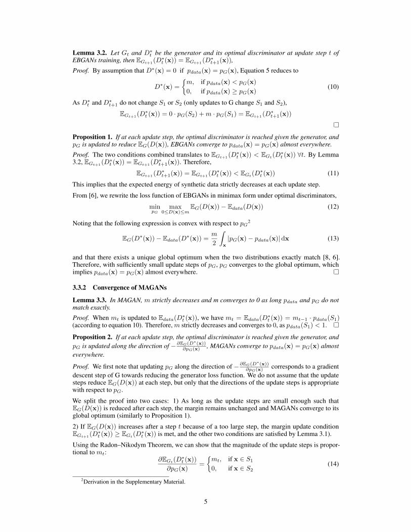
Figure 1: (a) MNIST generated samples distribution. The distribution shows relatively balancedgeneration among all 10 classes of the MNIST. (b) Noisy random generation using a fixed margin(equivalent to EBGANs). (c) Random generation from our proposed method. (b) and (c) differ onlyby the proposed adaptive margin.

This implies that the margin adaptation reduces the magnitude of the update steps, and as m strictlydecreases and converges to m∞ → 0 (according to Lemma 3.3), therefore it is guaranteed to find am small enough to meet the conditions of the first case above, specifically that the update steps aresufficiently small to reduce EG(D(x)) at each step.

While the effects of margin adaptation share some connections with learning rate decay from atheoretical standpoint, its empirical effects are subtler, as the adjustments are based on the on trainingstatistics. In particular, we hypothesize that margin adaptation maintains the equilibrium between thegenerator and the discriminator, which improves training stability and consequently the generatorperformance. Lowering the margin temporarily limits the power of the discriminator by removingmore synthetic samples from it loss function, until the generator catches up by generating moreconsistently samples with lower energies. At the same time, the margin reduction also protects thediscriminator from wasting model capacity on synthetic samples likely of low quality (i.e. of highenergy) and thus providing better gradients for the generator.

4 Experimental Results

For all experiments in this paper, we use a deep convolutional generator, analogous to DCGAN’s [14].For the discriminators, we use a fully-connected auto-encoder for the MNIST dataset, and a fullyconvolutional one forthe CIFAR-10 and the CelebA datasets. The convolutional auto-encoder iscomposed of strided convolution for encoding and fractional-strided convolutions for decoding. Allmodels are trained with Adamax [15] with a fixed learning rate of 0.0005, and momentum β1 of0.5, and a batch size of 64. Exact model architectures are reported separately for each dataset in theSupplementary Materials. The method requires no other techniques such as batch normalization [16],or layer-wise noises [8] to help with the training. We sample z from N (0, 1) and determine Nz suchthat the number of parameters in the discriminator and generator are roughly equal. The code usedfor the experiments is available on GitHub3.

4.1 Quantitative Evaluation

We first show that our method generates diverse samples with no mode collapse. In the first experiment,our architecture is trained on the MNIST dataset. A random mini-batch of samples is shown in Figure1c. To show that the model does not suffer from mode collapse, we trained a three-layer convolutionalclassifier on the MNIST separately (98.7% accuracy on MNIST test set) and used the classifier on50000 samples generated with our architecture. The results are shown in Figure 1a.

The results show that each of the 10 classes of MNIST is present, while 5 out of 10 classes aregenerated with a probability close to 10%, matching the original data distribution. The classes of"ones" and "twos" are respectively the most over and under-represented with 16.5% and 4.2% of the

3https://github.com/RuohanW/magan

6

(a) (b) (c)

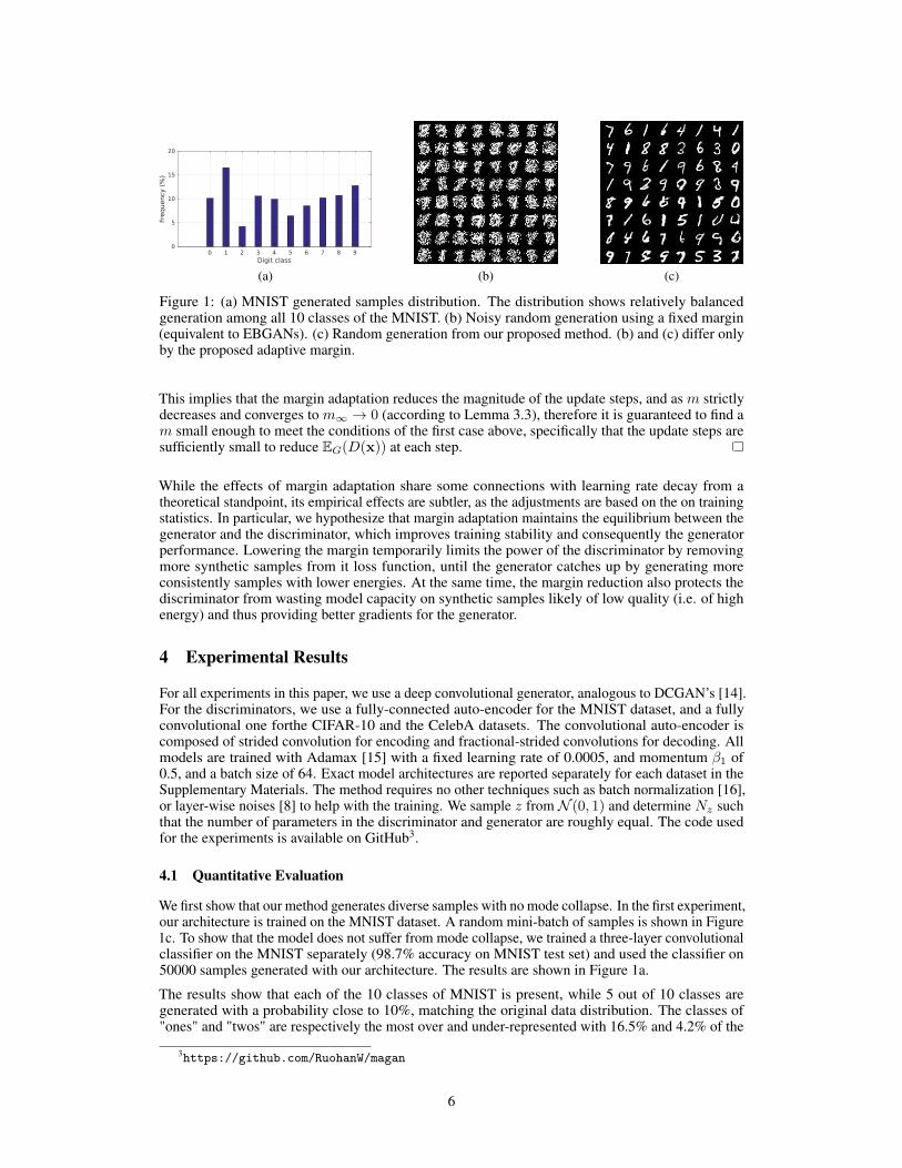
Figure 2: (a) EBGANs CelebA generation taken from [8]. (b) BEGANs CelebA generation basedon [21]. (c) CelebA generation from our method. Results from BEGANs and our method are froma random mini-batch of generates samples respectively. Best viewed in color and enlarged. Moresamples are available in the Supplementary Material.

distribution, which may be explained by the similarity between the "twos" and other classes, and thesimplicity of ones.

To quantify the sample diversity and quality of our results, we compute the inception score [7] on theMNIST samples generated by our architecture. The inception score is a heuristic commonly usedwith GANs to measure single sample quality and diversity using a standard pre-trained inceptionnetwork. We follow previous works to compute the score with 10 batches of 5000 independentgenerated samples, using the evaluation script from [7]. We emphasize that in order to compute theinception score for the MNIST, we replaced the pre-trained inception model with the aforementionedconvolutional MNIST classifier. To compare against EBGANs, we used code from [17], a EBGANsimplementation specifically tuned for MNIST generation. We report that our model achieves a scoreof 7.52±0.03 against 7.14±0.04 from EBGANs. The real samples from the MNIST test set achievesa score of 9.09± 0.08.

Table 1: CIFAR-10 Inception score compar-ison

Method Score ± Std

Real data 11.24± 0.12DFM [9] 7.72± 0.13EGANs [18] 7.07± 0.10BEGANs [13] 5.62ALI [19] (from [9]) 5.34± 0.05Improved GANs [7] 4.36± 0.04MIX + WGANs [20] 4.04± 0.07Wasserstein GANs [6] (from [20]) 3.82± 0.06MAGANs (proposed method) 6.40 ± 0.03

To further quantify the performance of our proposedarchitecture, we trained our model on the CIFAR-10dataset and computed the inception score. The result ispresented in Table 1, and compared against other state-of-the-art unsupervised GANs. For fair comparison, wedo not consider models using labeled data.

With the exception of Denoising Feature Matching(DFM) [9] (DFM) and EGAN [18], our method outper-forms all other methods by a large margin. Both DFMand EGANs introduces auxiliary training objectivesto improve the performance of the generator, whichare beyond the scope of this paper. Both works arecompatible with our framework and represent possibledirections for future investigations. Preliminary testshave shown promises in this direction.

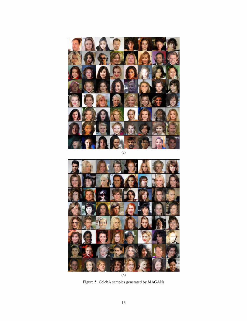
4.2 Qualitative Evaluation

For qualitative comparisons, we use the CelebA dataset, as generating realistic, highly detailed andflawless faces of different poses remains an open challenge in GANs. We compare the generationresults against those of BEGANs and EBGANs, as they are both state-of-the-art auto-encoder GANs,directly comparable to our method. For EBGANs, we directly use the results from [8]. For BEGANs,we use the code from [21], which is specifically tuned for the CelebA dataset, as the original paperdoes not release source code and used a private dataset. We also standardized the cropping of trainingimages for all the compared architectures.

7

0 0.5 1 1.5 2Number of steps #105

-1

0

1

2

3

4

Real lo

g e

nerg

y

EBGAN (m=10)EBGAN (m=5)EBGAN (m=1.08)MAGAN

(a) Comparison of real samples energy between pro-posed method and EBGAN

0 0.5 1 1.5 2Number of steps #105

-2

-1

0

1

2

3

Synth

eti

c lo

g e

nerg

y

EBGAN (m=10)EBGAN (m=5)EBGAN (m=1.08)MAGAN

(b) Comparison of synthetic samples energy betweenproposed method and EBGAN

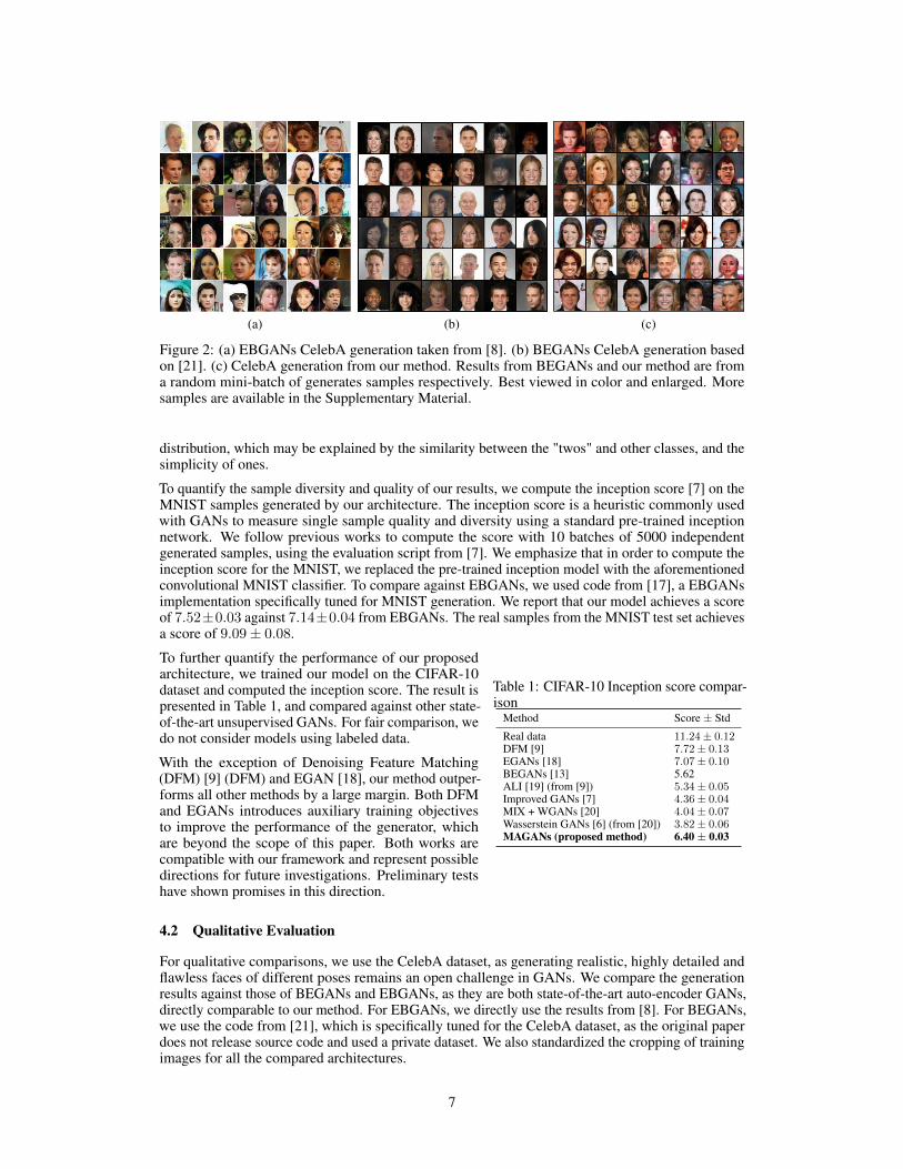
Figure 3: EBGANs have diverging energy for real and synthetic samples on the MNIST dataset. Theblack lines in (b) denotes EBGANs margins. The generator loss rises gradually and steadily abovethe preset margin. Real and synthetic data energy decreases in tandem in MAGANs. Best viewed incolor.

Compared against EBGANs, our results exhibit more detailed and coherent faces, and appear to bettercapture the symmetric property of faces and their appearances under different poses. Both EBGANsand our results show rich and diverse backgrounds, consistent with backgrounds contained in thetraining set. We follow closely to the parameter and architecture choices of EBGANs to attribute theimprovements in visual quality to the proposed margin adaptation.

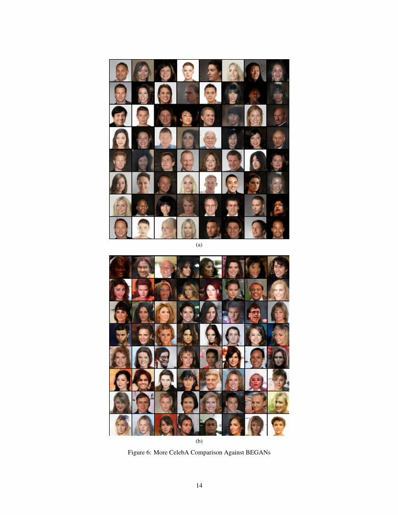
Our method generates very different samples compared to BEGANs. We first note that BEGANsresults are comparable to those presented in the original paper, with similar characteristics. BEGANsmostly generate uniform background between black and white, compare to the rich variety ofbackgrounds from the training data, and from our results. While both BEGANs and MAGANsgenerate visually appealing faces, our results demonstrate more diversity in terms of shape, hairstyleand color.

4.3 The Effects of Margin Adaptation

To further verify the effects of margin adaptation, we compared our method against EBGANs on theMNIST dataset, while keeping all other parameters and network architectures identical. We trainedthree EBGANs models by setting the margin at 10, 5 and 1.08 (the final margin value obtained byMAGANs) respectively. Figure 3 shows the evolutions of real and synthetic sample energy duringtraining, while Figure 1 shows the comparison of random samples generated from the two methods.All three EBGANs models produce samples of similar quality, shown in Figure 1b.

Qualitatively, the proposed method generates crisp and sharp samples, compared against the noisysamples produced by EBGANs. Quantitatively, real and synthetic sample energy decreases in tandemfor the proposed method. In contrast, the energies of real and synthetic samples diverge in EBGANs.In particular, the energy of synthetic samples, equivalent to the generator loss, does not decreasesover time, which causes difficulty in using the loss metric as an estimate of the training progress.Similar observations have been observed for standard GANs, whereby the Jensen-Shannon distancebetween the two distributions, a measure of similarity between two distributions, also worsen as thetraining proceeds [6]. Along with the qualitative and quantitative improvements demonstrated in theprevious sections, the results strongly suggest that margin adaptation improves both the stability andquality of GANs training.

5 Conclusion and Future Work

We have presented Margin Adaptation for GANs, a novel training procedure for auto-encoder GANs.We have shown theoretically that margin adaptation allows GANs to converge under more generalconditions, which improves training stability and both qualitative and quantitative performancecompared to the state-of-the-art. For future work, we wish to explore the use of margin adaptation inother GANs frameworks to test its general applicability.

8

References[1] Ian Goodfellow, Jean Pouget-Abadie, Mehdi Mirza, Bing Xu, David Warde-Farley, Sherjil

Ozair, Aaron Courville, and Yoshua Bengio. Generative adversarial nets. In Advances in neuralinformation processing systems, 2014.

[2] Christian Ledig, Lucas Theis, Ferenc Huszar, Jose Caballero, Andrew P. Aitken, Alykhan Tejani,Johannes Totz, Zehan Wang, and Wenzhe Shi. Photo-realistic single image super-resolutionusing a generative adversarial network. CoRR, abs/1609.04802, 2016.

[3] Alex Kuefler, Jeremy Morton, Tim Allan Wheeler, and Mykel John Kochenderfer. Imitatingdriver behavior with generative adversarial networks. CoRR, abs/1701.06699, 2017.

[4] Ashish Shrivastava, Tomas Pfister, Oncel Tuzel, Josh Susskind, Wenda Wang, and RussWebb. Learning from simulated and unsupervised images through adversarial training. CoRR,abs/1612.07828, 2016.

[5] Ian Goodfellow. NIPS 2016 tutorial: Generative adversarial networks. CoRR, abs/1701.00160,2017.

[6] Martin Arjovsky, Soumith Chintala, and Léon Bottou. Wasserstein gan. arXiv:1701.07875,2017.

[7] Tim Salimans, Ian Goodfellow, Wojciech Zaremba, Vicki Cheung, Alec Radford, and Xi Chen.Improved techniques for training gans. In Advances in Neural Information Processing Systems,2016.

[8] Junbo Zhao, Michael Mathieu, and Yann LeCun. Energy-based generative adversarial network.International Conference on Learning Representations, 2017.

[9] D Warde-Farley and Y Bengio. Improving generative adversarial networks with denoisingfeature matching. International Conference on Learning Representations, 2017.

[10] Ishaan Gulrajani, Faruk Ahmed, Martin Arjovsky, Vincent Dumoulin, and Aaron Courville.Improved training of wasserstein gans. arXiv preprint arXiv:1704.00028, 2017.

[11] Pascal Vincent, Hugo Larochelle, Yoshua Bengio, and Pierre-Antoine Manzagol. Extractingand composing robust features with denoising autoencoders. In International Conference onMachine Learning, 2008.

[12] Anh Nguyen, Jason Yosinski, Yoshua Bengio, Alexey Dosovitskiy, and Jeff Clune. Plug &play generative networks: Conditional iterative generation of images in latent space. CoRR,abs/1612.00005, 2016.

[13] D. Berthelot, T. Schumm, and L. Metz. BEGAN: Boundary Equilibrium Generative AdversarialNetworks. ArXiv e-prints, March 2017.

[14] Alec Radford, Luke Metz, and Soumith Chintala. Unsupervised representation learning withdeep convolutional generative adversarial networks. CoRR, abs/1511.06434, 2015.

[15] Diederik P. Kingma and Jimmy Ba. Adam: A method for stochastic optimization. InternationalConference for Learning Representations, 2015.

[16] Sergey Ioffe and Christian Szegedy. Batch normalization: Accelerating deep network trainingby reducing internal covariate shift. In Proceedings of the 32nd International Conference onMachine Learning, 2015.

[17] Namju Kim. A tensorflow implementation of Junbo et al’s Energy-based generative adversarialnetwork ( EBGAN ) paper. https://github.com/buriburisuri/ebgan, 2016.

[18] Zihang Dai, Amjad Almahairi, Philip Bachman, Eduard Hovy, and Aaron Courville. Cali-brating energy-based generative adversarial networks. International Conference for LearningRepresentations, 2017.

9

[19] V. Dumoulin, I. Belghazi, B. Poole, O. Mastropietro, A. Lamb, M. Arjovsky, and A. Courville.Adversarially Learned Inference. ArXiv e-prints, June 2016.

[20] S. Arora, R. Ge, Y. Liang, T. Ma, and Y. Zhang. Generalization and Equilibrium in GenerativeAdversarial Nets (GANs). ArXiv e-prints, March 2017.

[21] Taehoon Kim. Tensorflow implementation of "BEGAN: Boundary Equilibrium GenerativeAdversarial Networks". https://github.com/carpedm20/BEGAN-tensorflow, 2017.

AppendicesA Technical Details for Section 3.3.1

We show that EG(D∗(x))− Edata(D

∗(x)) = m2

∫x|pG(x)− pdata(x)|dx.

Proof. we first show that∫S1(pG(x)− pdata(x)) dx = 1

2

∫x|pG(x)− pdata(x)|dx∫

S1

(pG(x)− pdata(x)) dx+

∫S2

(pG(x)− pdata(x)) dx = 0∫S1

(pG(x)− pdata(x)) dx =

∫S2

(pdata(x)− pG(x)) dx∫S1

|pG(x)− pdata(x)|dx =

∫S2

|pG(x)− pdata(x)|dx∫S1

|pG(x)− pdata(x)|dx =1

2(

∫S1

|pG(x)− pdata(x)|dx+

∫S2

|pG(x)− pdata(x)|dx)∫S1

(pG(x)− pdata(x)) dx =1

2

∫x

|pG(x)− pdata(x)|dx

Therefore,

EG(D∗(x))− Edata(D

∗(x)) = m

∫S1

(pG(x)− pdata(x)) dx

=m

2

∫x

|pG(x)− pdata(x)|dx

B Supplementary Details for Experimental Setups

We use FC, CV and DC to denote fully-connected, convolution and deconvolution layers. Forexample, FC(128) denotes a fully-connected layer with a 128-unit output. CV(64, 4c2s) denotesa convolution layer with 64 output feature maps, using 4x4 kernels with stride 2. DC are definedsimilarly as CV.

B.1 MNIST Experiment

Discriminator: Input-FC(256)-FC(256)-FC(784)

Generator: Input-DC(128, 7c1s)-DC(64, 4c2s)-DC(1, 4c2s)

We set Nz = 50, to roughly balance the network capacity of the generator and the discriminator.All internal activations use RELU units while the output layers of both the discriminator and thegenerator use sigmoid units. The same architecture is used for Section 4.3.

10

B.2 CelebA Experiment

Discriminator: Input-CV(64, 4c2s)-CV(128, 4c2s)-CV(256, 4c2s)-CV(512, 4c2s)-DC(256, 4c2s)-DC(128, 4c2s)-DC(64, 4c2s)-DC(3, 4c2s)

Generator: Input-DC(512, 4c1s)-DC(256, 4c2s)-DC(128, 4c2s)-DC(64, 4c2s)-DC(3, 4c2s)

We set Nz = 350 to approximately balance the capacity of the two networks. The discriminator usesLeakly RELU for internal activations, while the generator uses RELU. The output layers of bothnetworks use tanh units.

B.2.1 CIFAR-10 Experiment

Discriminator: Input-CV(64, 3c1s)-CV(128, 3c2s)-CV(128, 3c1s)-CV(256, 3c2s)-CV(256, 3c1s)-CV(512, 3c2s)-DC(256, 3c2s)-DC(256, 3c1s)-DC(128, 3c2s)-DC(128, 3c1s)-DC(64, 3c2s)-DC(3,3c1s)

Generator: Input-DC(512, 4c1s)-DC(256, 3c2s)-DC(256, 3c1s)-DC(128, 3c2s)-DC(128, 3c1s)-DC(64, 3c2s)-DC(3, 3c1s)

We set Nz = 320. The discriminator uses Leakly RELU for internal activations, while the generatoruses RELU. The output layers of both networks use tanh units.

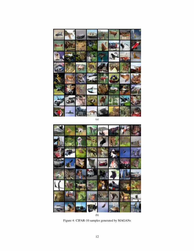
C Additional Generated Samples For CIFAR-10 and CelebA

All samples shown below are random mini-batches of size 64.

11

(a)

(b)

Figure 4: CIFAR-10 samples generated by MAGANs

12

(a)

(b)

Figure 5: CelebA samples generated by MAGANs

13

(a)

(b)

Figure 6: More CelebA Comparison Against BEGANs

14