ABSTRACT ALGORITHMS AND COMPLEXITY …cs.pnw.edu/~hairong/papers/hairong-thesis.pdf · ABSTRACT...

ABSTRACT

ALGORITHMS AND COMPLEXITY ANALYSES FOR SOMECOMBINATORIAL OPTIMIZATION PROBLEMS

byHairong Zhao

The main focus of this dissertation is on classical combinatorial optimization problems in

two important areas: scheduling and network design.

In the area of scheduling, the main interest is in problems in the master-slave model.

In this model, each machine is either a master machine or a slave machine. Each job is

associated with a preprocessing task, a slave task and a postprocessing task that must be

executed in this order. Each slave task has a dedicated slave machine. All the preprocessing

and postprocessing tasks share a single master machine or the same set of master machines.

A job may also have an arbitrary release time before which the preprocessing task is not

available to be processed. The main objective in this dissertation is to minimize the total

completion time or the makespan. Both the complexity and algorithmic issues of these

problems are considered. It is shown that the problem of minimizing the total completion

time is strongly NP-hard even under severe constraints. Various efficient algorithms are

designed to minimize the total completion time under various scenarios.

In the area of network design, the survivable network design problems are studied

first. The input for this problem is an undirected graph

, a non-negative cost for

each edge, and a nonnegative connectivity requirement for every (unordered) pair of

vertices , . The goal is to find a minimum-cost subgraph in which each pair of vertices

, is joined by at least edge (vertex)-disjoint paths. A Polynomial Time Approxi-

mation Scheme (PTAS) is designed for the problem when the graph is Euclidean and the

connectivity requirement of any point is at most . PTASs or Quasi-PTASs are also de-

signed for -edge-connectivity problem and biconnectivity problem and their variations in

unweighted or weighted planar graphs.

Next, the problem of constructing geometric fault-tolerant spanners with low cost

and bounded maximum degree is considered. The first result shows that there is a greedy

algorithm which constructs fault-tolerant spanners having asymptotically optimal bounds

for both the maximum degree and the total cost at the same time. Then an efficient algo-

rithm is developed which finds fault-tolerant spanners with asymptotically optimal bound

for the maximum degree and almost optimal bound for the total cost.


byHairong Zhao

A DissertationSubmitted to the Faculty of

New Jersey Institute of Technologyin Partial Fulfillment of the Requirements for the Degree of

Doctor of Philosophy in Computer Sciences

Department of Computer Science

May 2005

Copyright c

2005 by Hairong Zhao

ALL RIGHTS RESERVED

APPROVAL PAGE


Hairong Zhao

Dr. Joseph Leung, Dissertation Co-Advisor DateDistinguished Professor of Computer Science, New Jersey Institute of Technology

Dr. Artur Czumaj, Dissertation Co-Advisor DateAssociate Professor of Computer Science, New Jersey Institute of Technology

Dr. Teunis J. Ott, Committee Member DateProfessor of Computer Science, New Jersey Institute of Technology

Dr. Wojciech Rytter, Committee Member DateProfessor of Computer Science, New Jersey Institute of Technology

Dr. Clifford Stein, Committee Member DateProfessor of Industrial Engineering and Operations Research, Columbia University

BIOGRAPHICAL SKETCH

Author: Hairong Zhao

Degree: Doctor of Philosophy

Date: May 2005

Date of Birth: September 07, 1972

Place of Birth: Shanxi, People’s Republic of China

Undergraduate and Graduate Education:

Doctor of Philosophy in Computer Science,New Jersey Institute of Technology, Newark, NJ, 2005

Master of Computer Science,Beijing University of Posts & Telecommunications, Beijing, China, 1997

Bachelor of Computer Science,Taiyuan University of Technology, Shanxi, China, 1994

Major: Computer Science

Presentations and Publications:

J. Y-T. Leung and H. Zhao, “Minimizing Mean Flowtime and Makespan on Master-SlaveSystems,” Journal of Parallel and Distributed Computing, accepted for publication.

J. Y-T. Leung and H. Zhao, “Minimizing Mean Flowtime on Master-Slave Machines,” Pro-ceedings of the 2004 International Conference on Parallel and Distributed ProcessingTechniques and Applications, vol. 2, pp. 939-945, 2004.

A. Czumaj, M. Grigni, P. A. Sissokho, and H. Zhao “Approximation Schemes for Minimum2-Edge-Connected and Biconnected Subgraphs in Planar Graphs,” Proceedings of the15th Annual ACM-SIAM Symposium on Discrete Algorithms, pages 489 - 498, 2004.

A. Czumaj and H. Zhao “Fault-Tolerant Geometric Spanners,” Discrete and ComputationalGeometry, Vol. 32, pp. 207-230, 2004.

A. Czumaj and H. Zhao “Fault-Tolerant Geometric Spanners,” Proceedings of the 19thACM Symposium on Computational Geometry, pp. 1-10, 2003.

J. Y-T. Leung and H. Zhao “Real-Time Scheduling Analysis,” Final report to Federal Avi-ation Administration, 2003.

iv

A. Czumaj, A. Lingas, and H. Zhao “ Polynomial-Time Approximation Schemes for theEuclidean Survivable Network Design Problem, ” Proc. of the 29th International Col-loquium on Automata, Languages and Programming (ICALP’02) , pp. 973-984, 2002.

A. Berger, A. Czumaj, M. Grigni and H. Zhao. “Approximate Minimum 2-Connected Sub-graphs in Weighted Planar Graphs,” submitted.

A. Czumaj, W. Rytter, X. Wang and H. Zhao, “A Linear-Time Algorithm for 3-Path Color-ing of 2-Regular Digraphs,” submitted.

A. Berger, M. Grigni and Hairong Zhao, “A Well-Connected Separator for Planar Graphs,”submitted.

Y. Huo, J. Y-T. Leung and H. Zhao, “Complexity of Two Dual Criteria Scheduling Prob-lems,” submitted.

Y. Huo, J. Y-T. Leung and H. Zhao, “Bi-criteria Scheduling Problems: Number of TardyJobs and Maximum Weighted Tardiness,” submitted.

J. Y-T. Leung and H. Zhao, “Minimizing Total Completion Time in Master-Slave Systems,”submitted.

H. Zhao, “Survivable Network Design and Fault Tolerant Spanners,” invited talk at LosAlamos National Laboratory, March, 2005.

H. Zhao, “Minimizing Mean Flowtime and Makespan on Master-Slave Systems,” invitedtalk at INFORMS Annual Meeting, October 2004.

H. Zhao, “Fault Tolerant Spanners and Their Applications,” DIMACS/CS Light Seminar:Theoretical Computer Science, DIMACS Center, Rutgers Universe, March, 2004.

H. Zhao, “Approximation Schemes for Minimum 2-Edge-Connected and Biconnected Sub-graphs in Planar Graphs,” presentation at SODA 2004, New Orleans, January, 2004.

H. Zhao, “Fault-Tolerant Geometric Spanners,” DIMACS Workshop on Computational Ge-ometry, DIMACS Center, Rutgers University, November, 2002.

v

This dissertation is dedicated to my parents. Theirsupport, encouragement, and constant love havesustained me throughout my life.

vi

ACKNOWLEDGMENT

I have been very lucky to have two great advisors during my graduate study in NJIT –

Joseph Leung and Artur Czumaj. Without their support, patience and encouragement, this

dissertation would not exist.

I sincerely thank Joseph Leung for bringing my attention to the field of computa-

tional complexity and scheduling theory in the first place. I am grateful for his generous

support during my study. I thank him for spending a great deal of valuable time giving me

technical and editorial advice for my research. I am deeply indebted to Artur Czumaj, who

is not only an advisor, but also a mentor and a friend. I am grateful to him for teaching me

much about research and scholarship, for giving me invaluable advice on presentations and

writings among many other things, for many enjoyable and encouraging discussions with

him.

My thanks also go to the members of my dissertation committee, Cliff Stein, Teunis

Ott and Wojciech Rytter, for reading previous drafts of this dissertation and providing many

valuable comments that improved the contents of this dissertation. I must also thank my

coauthors, Artur Czumaj, Joseph Leung, Michelangelo Grigni, Wojciech Rytter, Andre

Berger, Andrzej Lingas, Xin Wang, Yumei Huo and Papa Sissokho. It has been such a

wonderful experience to work with each of them. Although I have not even had a chance

to meet some of them, each has taught me a great deal about research and about writing

research.

I am also grateful to my colleagues, Haibing Li, Yumei Huo and Xin Wang for nu-

merous interesting and good-spirited discussions about research. The friendship of Jingx-

uan Liu, Binghu Zhang, Hong Zhao, Yayi Hu, Sen Zhang, Min Zhang, Chang Liu, Thoa

Hoang, is much appreciated. They have given me not only advice on research in general,

but also valuable suggestions about life, living and job hunting, etc. I must give my thanks

to my best friends in my life, Qingrui Ping, Li Gao, Xiangping Wei. They are more than

vii

friends, they are part of my family. Though they are far away from me, their support is al-

ways with me. Their sincere care for me and my family is a treasure of my life. I thank

Maryann McCoul for her trust in me and for her great advice when I needed it the most.

Last, I would like to thank my husband, Wenxin Mao, for his understanding and

love during the past few years. His support and encouragement were in the end what made

this dissertation possible. I give my deepest gratitude to my parents for their endless love

and support which provided the foundation for this work. I also thank my dearest brother

and sister for their love and for taking care of my parents during my absence.

This work is supported in part by NSF Grant DMI-0300156 and by FAA Grant

01-C-AW-NJIT.

viii

TABLE OF CONTENTS

"! #$%& 1 INTRODUCTION '(''(')')')')')')')')')')')')')')')')')')')'(''(''(''(''(' 1

1.1 Machine Scheduling Problems '(''(''(''(''(''(''(')')')')')')')')')' 2

1.2 Network Design Problems ')')')')')')')')')')')')')')')'(''(''(''(''(' 5

1.3 Outline ''(''(''(')')')')')')')')')')')')')')')')')')')'(''(''(''(''(' 9

PART I: SCHEDULING PROBLEMS IN MASTER-SLAVE MODEL ')')')')')' 12

2 COMPLEXITY OF SCHEDULING PROBLEMS IN MASTER-SLAVE MODEL 13

2.1 Master-slave Model ''(''(''(''(''(''(''(''(''(')')')')')')')')'(' 13

2.2 Applications of Master-slave Model ''(''(''(''(''(')')')')')')')')')' 14

2.3 Scheduling Problems in Master-slave Model: Definitions and Notations ')' 16

2.4 Previous Work ')')'(''(''(''(''(''(''(''(''(''(')')')')')')')')')' 18

2.5 New Results: Complexity of Scheduling Problems in Master-slave Model ' 20

3 OPTIMAL AND APPROXIMATION ALGORITHMS: SPECIAL CASES ''(' 30

3.1 Optimal Algorithms for * +, : Canonical and Order Preserving Schedules ' 30

3.2 Approximation Algorithms for * +-, : Canonical Schedules ')')')')')')')' 31

3.3 Approximation Algorithms for No-wait-in Makespan '(')')')')')')')')')' 40

4 APPROXIMATION ALGORITHMS: GENERAL CASES ''(')')')')')')')')')' 48

4.1 Preliminaries '(''('(''(''(''(''(''(''(''(''(''(')')')')')')')')')' 48

4.2 New Results and Techniques ''(''(''(''(''(''(''(')')')')')')')')')' 50

4.3 Single-master ''('(''(''(''(''(''(''(''(''(''(')')')')')')')')')' 51

4.3.1 Canonical Preemptive Schedules ''(''(''(''('(''(''(''(''(' 51

4.3.2 Non-canonical Preemptive Schedules ')')')')')')'(''(''(''(''(' 54

4.3.3 Arbitrary Release Times ')')')')')')')')')')')')'(''(''(''(''(' 56

4.4 Multi-master '(''(')')')')')')')')')')')')')')')')')')')'(''(''(''(''(' 57

4.4.1 Non-canonical Preemptive Schedules ')')')')')')'(''(''(''(''(' 57

4.4.2 Arbitrary Release Times ')')')')')')')')')')')')'(''(''(''(''(' 59

ix

TABLE OF CONTENTS(Continued) "! #$%&

4.5 Distinct Preprocessing and Postprocessing Masters '(''(')')')')')')')')')' 62

4.6 Converting Preemptive Schedules into Non-preemptive Schedules ')')')')' 65

4.6.1 Single Master and Multi-Master Systems ''(''('(''(''(''(''(' 67

4.6.2 Distinct Preprocessors and Postprocessors ')')')'(''(''(''(''(' 70

4.7 Linear Programming: Distinct Preprocessors and Postprocessors '(''(''(' 72

4.7.1 .0/ .21 43 '(''(''(''(''(''(''(''(''(')')')')')')')')')' 73

4.7.2 .0/65 3 and .2175 3 ''(''(''(''(''(''(''(')')')')')')')')')' 76

PART II: NETWORK DESIGN PROBLEMS '(''(''(''(''('(''(''(''(''(' 78

5 POLYNOMIAL-TIME APPROXIMATION SCHEMES FOR THE EUCLIDEANSURVIVABLE NETWORK DESIGN PROBLEM ')')')')'(''(''(''(''(' 79

5.1 Introduction ')')')'(''(''(''(''(''(''(''(''(''(')')')')')')')')')' 79

5.1.1 Related Works '(''(''(''(''(''(''(''(''('(''(''(''(''(' 79

5.1.2 New Contributions ')')')')')')')')')')')')')')')'(''(''(''(''(' 80

5.2 Definitions ''(''(')')')')')')')')')')')')')')')')')')')'(''(''(''(''(' 81

5.3 Steiner Minimum Tree Problem ')')')')')')')')')')')')'(''(''(''(''(' 86

5.4 Filtering for SMT '('(''(''(''(''(''(''(''(''(''(')')')')')')')')')' 87

5.4.1 First Filtering Property '(''(''(''(''(''(''('(''(''(''(''(' 89

5.4.2 Second Filtering Property ')')')')')')')')')')')')'(''(''(''(''(' 98

5.4.3 Complexity of SMT-Filtering ')')')')')')')')')')'(''(''(''(''(' 100

5.5 Lightening for SMT ''(''(''(''(''(''(''(''(''(')')')')')')')')')' 101

5.6 Searching for SMT '(''(''(''(''(''(''(''(''(''(')')')')')')')')')' 106

5.7 Polynomial-Time Approximation Scheme for SMT ')')'(''(''(''(''(' 108

5.8 8:9 3" "; -Connectivity Problem ')')')')')')')')')')')')')'(''(''(''(''(' 109

5.8.1 Lightening for 8<9 3" "; -Edge-Connectivity '(''('(''(''(''(''(' 109

5.8.2 Dynamic Programming for 8:9 3" "; -Edge-Connectivity ')')')')')')' 110

5.9 Extensions ''(''('(''(''(''(''(''(''(''(''(''(')')')')')')')')')' 114

x


5.10 Auxiliary Claims ')'(''(''(''(''(''(''(''(''(''(')')')')')')')')')' 115

6 APPROXIMATION SCHEMES FOR MINIMUM 2-EDGE-CONNECTED ANDBICONNECTED SUBGRAPHS IN PLANAR GRAPHS ')'(''(''(''(''(' 117

6.1 Introduction ')')')'(''(''(''(''(''(''(''(''(''(')')')')')')')')')' 117

6.2 Cuts and = -EC Types ''(''(''(''(''(''(''(''(''('(''(''(''(''(' 119

6.3 Planar Separators ')'(''(''(''(''(''(''(''(''(''(')')')')')')')')')' 123

6.4 The -ECSS Algorithm '(''(''(''(''(''(''(''(''(')')')')')')')')')' 125

6.5 The -VCSS Algorithm ''(''(''(''(''(''(''(''(')')')')')')')')')' 130

6.5.1 Types of ( -VC, P)-Safe Planar Graphs '(''(''('(''(''(''(''(' 131

6.5.2 Recursive Decomposition ''(''(''(''(''(''(')')')')')')')')')' 137

6.5.3 Dynamic Programming ')')')')')')')')')')')')')'(''(''(''(''(' 139

7 APPROXIMATION SCHEMES FOR MINIMUM 2-CONNECTED SPANNINGSUBGRAPHS IN WEIGHTED PLANAR GRAPHS ')')')'(''(''(''(''(' 142

7.1 Introduction ')')')'(''(''(''(''(''(''(''(''(''(')')')')')')')')')' 142

7.1.1 Related Results '(''(''(''(''(''(''(''(''('(''(''(''(''(' 142

7.1.2 New Contributions and Techniques ')')')')')')')'(''(''(''(''(' 143

7.2 PTAS for the 2-ECSSM Problem ')')')')')')')')')')')')'(''(''(''(''(' 145

7.3 Augmented Planar Spanners ''(''(''(''(''(''(''(')')')')')')')')')' 146

7.4 Spanners and 2-EC Subgraphs '(''(''(''(''(''(''(')')')')')')')')')' 149

7.5 Approximation Schemes for the 2-ECSS and 2-VCSS Problems '(''(''(' 151

7.6 Extensions to the 8 3" "; -Connectivity Problem ')')')')')'(''(''(''(''(' 153

8 FAULT-TOLERANT GEOMETRIC SPANNERS ')')')')')')'(''(''(''(''(' 156

8.1 Introduction ')')')'(''(''(''(''(''(''(''(''(''(')')')')')')')')')' 156

8.1.1 Previous Results ''(''(''(''(''(''(''(''('(''(''(''(''(' 156

8.1.2 New Contributions ')')')')')')')')')')')')')')')'(''(''(''(''(' 158

8.2 Preliminaries '(''('(''(''(''(''(''(''(''(''(''(')')')')')')')')')' 160

xi


8.2.1 Menger’s Theorem and Its Consequences ''(''(')')')')')')')')')' 160

8.3 = -Vertex Fault-Tolerant Spanners of Low Degree and Low Cost '(''(''(' 161

8.3.1 Analyzing the Maximum Degree ''(''(''(''('(''(''(''(''(' 162

8.3.2 Upper Bound for the Cost of Spanners Generated by the = -GreedyAlgorithm ')')')')')')')')')')')')')')')')')')'(''(''(''(''(' 165

8.4 Efficient Construction of Fault Tolerant Spanners ')')')'(''(''(''(''(' 167

8.4.1 Basic Auxiliary Properties ')')')')')')')')')')')'(''(''(''(''(' 168

8.4.2 Sufficient Conditions for Being a = -Vertex Fault-Tolerant Spanner ' 169

8.4.3 Efficient Construction of = Fault-Tolerant Spanner ')')')')')')')')' 175

9 CONCLUSIONS ''(''(')')')')')')')')')')')')')')')')')')')'(''(''(''(''(' 185

9.1 Scheduling Problems ')')')')')')')')')')')')')')')')')'(''(''(''(''(' 185

9.2 Network Design Problems ')')')')')')')')')')')')')')')'(''(''(''(''(' 186

REFERENCES ')')')')')')'(''(''(''(''(''(''(''(''(''('(''(''(''(''(' 191

xii

LIST OF TABLES

> ?A@B #$%& 4.1 New Results for Single-Master System ''(''(''(''(''(')')')')')')')')')' 51

4.2 New Results for Multi-Master System, All Schedules are Non-Canonical ''(' 51

4.3 New Results for Distinct Preprocessor and Postprocesor System, .C/ .D1 E3 52

4.4 New results for distinct preprocessor and postprocesor, .C/65 3 and .2175 3 ' 52

xiii

LIST OF FIGURES

FHG %JIK!L #$%& 2.1 An illustration of the optimal schedule in the proof of Theorem 2.5.2. ''(''(' 22

2.2 An illustration of the optimal schedule in the proof of Theorem 2.5.4. ''(''(' 24

2.3 An illustration of the optimal schedule in the proof of Theorem 2.5.5. ''(''(' 25

3.1 Illustration of Algorithm 1. ')')')')')')')')')')')')')')')')'(''(''(''(''(' 40

3.2 Illustration of Algorithm 2. ')')')')')')')')')')')')')')')')'(''(''(''(''(' 43

3.3 Illustration of the proof of Theorem 3.3.3. ')')')')')')')')'(''(''(''(''(' 43

4.1 Convert a preemptive schedule into a non-preemptive schedule. ')')')')')')')' 69

5.1 Dissection of a bounding cube in M 1 ''(''(''(''(''(''(')')')')')')')')')' 86

5.2 Illustration of connectivity type construction. '(''(''(''(')')')')')')')')')' 111

5.3 Illustration to the proof of Lemma 5.10.1. ')')')')')')')')')'(''(''(''(''(' 115

6.1 The three different types of the separator. ')')')')')')')')')'(''(''(''(''(' 125

6.2 Type of a2 N + PO -safe graph used in the 2-VCSS Algorithm ')')')')')')' 141

7.1 A non-simple face Q in R , a chord S , and walksO / and

O 1 . ')')')')')')')')')' 147

7.2 (a) Face Q of RT (oval) with chord U , pathOWV

(bold), and chords removed fromXby the chord move at U (dotted). (b) Face Q with a face-edge S (dashed)

crossed by five chords fromX

. ')')')')')')')')')')')')')'(''(''(''(''(' 150

8.1 Any Y[Z\^] for points in _/ and _J1 must have weight at least `badc 1^e , while the MSThas weight fgaih e . ''('(''(''(''(''(''(''(''(''(''(')')')')')')')')')' 159

8.2 The = -Gap-Greedy Algorithm ')')')')')')')')')')')')')')')'(''(')')')')')')' 172

9.1 Light spanners do not always exist '(''(''(''(''(''(''(')')')')')')')')')' 189

9.2 Greedy algorithm does not always find light spanners of planar graphs '(''(' 189

xiv

CHAPTER 1

INTRODUCTION

A combinatorial optimization problem is concerned with selecting, from among a finite

set of possible solutions, the one that maximizes or minimizes a certain function, the so-

called objective function. Such problems are of great importance because a large number

of practical problems in various fields can be formulated as combinatorial optimization

problems: for example, inventory control, the scheduling of lines in flexible manufacturing

facilities, planning communication in traffic networks, finding the shortest or most reliable

paths in traffic or communication networks, etc. Extensive surveys of related applications

of combinatorial optimization are given in [49], [60].

Because of its importance, combinatorial optimization has attracted a great deal

of research effort and has experienced a particularly fast development during the last few

decades. Given any specific optimization problem of interest, the first question that arises

is whether there exists an efficient (polynomial-time) algorithm. While some problems in

this area are relatively well understood and have known efficient algorithms, many others

are intractable, typically NP-hard, e.g. scheduling problems, partitioning problems. So

under the widely believed assumption thatOCjlkmO

, there is no hope of getting polynomial

time algorithms for solving these problems.

However, very large instances of these problems frequently arise in practice. Thus,

one is forced to look for algorithms that run in polynomial time and hopefully return a near-

optimal solution. Such algorithms are called approximation algorithms. An approximation

algorithm is called an n -approximation algorithm for a problem o , if for any instance p of

o , it always returns a solution with value at most (at least for maximization problems) ntimes the optimal. The value n is called the approximation ratio or the performance ratio of

the algorithm. Of course, one hopes that n is as close to3

as possible. However, it turns out

1

2

that different NP-hard problems exhibit different approximability properties. Some prob-

lems, e.g. the knapsack problem, allow a polynomial-time approximation scheme (PTAS);

i.e., a family of algorithms 8rqtsr; such that, for each fixed uDvw9 , 8rqts:; runs in time poly-

nomial in the size of the input and produces a<36x u -approximation. On the other hand,

some other problems have intrinsic limitations to approximability. For example, there is no

PTAS for the general traveling salesman problem unlessOylkzO

.

This dissertation focuses on classical combinatorial optimization problems in two

important areas: scheduling and network design. Not surprisingly, most of these prob-

lems have been or will be shown in this dissertation to be NP-hard. Thus, various constant

approximation algorithms or approximation schemes are designed throughout the disserta-

tion.

1.1 Machine Scheduling Problems

Scheduling is an intensively studied class of discrete optimization problems. Scheduling

problems are motivated by the allocation of limited resources to jobs over time, subject to

some constraints. It is a decision-making process with the goal of optimizing one or more

objectives. The resources and jobs can take on many different forms. The resource can

be machines in a workshop, runways at an airport, processing units in a computing envi-

ronment. The jobs can be operations in a workshop, takeoffs and landings of air planes or

computer programs. Standard scheduling requirements include: a job cannot be processed

by two or more machines at a time, or a machine cannot process two or more jobs at the

same time. Depending on the type of scheduling system, specific constraints should be sat-

isfied. For example, jobs may have different release times and deadlines, different jobs may

have different priorities, a job may not be allowed to preempt other jobs, etc. The objective

can also take on many different forms; e.g., minimizing the makespan (the maximum com-

pletion time among all jobs) or the total completion time or the maximum response time,

3

or maximizing the number of on time jobs. For an extensive introduction into the theory of

scheduling, see, e.g., [7], [22], [76], [96].

Although scheduling problems may concern different types of resources, many of

them can be modeled as scheduling jobs on machines. A schedule specifies, for each

time instant, the set of jobs executing at that instant, and the machines on which they are

executing.

Depending on the properties of the jobs, the number and type of machines, and

the optimization goal, there are various problems under different models. In the simplest

model, there is a single machine and jobs, each of which is ready at time 9 and must be

executed without interruption. In a complex model, there are different types of machines;

each job has several tasks which have to be executed on different machines and may be in

certain order. These models are known as shop models. In the open shop model, there is

no restriction on the order of the tasks. In the flow shop model, each job has exactly one

task that needs to be processed in each machine, and the tasks of each job must follow the

same order. In the job shop model, each job has its own ordering of the tasks, and several

tasks can visit the same machine.

Scheduling problems in master-slave model. Scheduling problems in the master-slave

model was recently introduced by Sahni [104]. In this model there are jobs and . ma-

chines. Each job is associated with a preprocessing task, a slave task and a postprocessing

task that must be executed in this order. Each machine is either a master machine or a slave

machine. While the preprocessing and postprocessing tasks are scheduled on the master

machine, each slave task is scheduled on a dedicated slave machine.

The master-slave model is closely related to the two-machine flow shop model with

transfer lags. In this flow shop model, each job | has two operations: the first operation is

scheduled on the upstream machine and the second operation is scheduled on the down-

stream machine. The interval or time lag between the finish time of the first operation and

4

the start time of the second operation must be exactly or at least ~, . If the r, ’s are large

enough such that all of the first operations finish before the start of any second operation,

then the flow shop problem is equivalent to the problem of scheduling on a single machine

with time lags and two tasks per job, subject to the constraint that all of the first opera-

tions are scheduled first. The latter problem is identical to the single-master master-slave

scheduling model.

The master-slave model finds many applications in parallel computer scheduling

and industrial settings such as semiconductor testing, machine scheduling, transportation

maintenance, etc.; see [104], [106], [105], [115]. For example, suppose there is a main

thread running on one processor whose function is to prepare data then fork and initiate new

child threads that do the computations on different processors. After the computation of a

child thread, the main thread collects the computation results and performs some processing

on the results. Here, each child thread can be seen as a job with three tasks: the thread

initiation and data preparation is the preprocessing task, the computation is the slave task

and the postprocessing of the results from the computation is the postprocessing task.

The main objective in this dissertation is to minimize the total completion time or

makespan under various scenarios. First, it is shown that many of the problems are NP-

hard in the strong sense. Then some special cases are considered. It is assumed that (1)

there is a single master, (2) all jobs have the same release time 9 , same preprocessing

task length and same postprocessing task length U ; i.e. the jobs are different from each

other only by their slave tasks, (3) no preemption is allowed. Optimal or approximation

algorithms are developed for some problems in this case. Finally, more general cases are

considered. A job can have an arbitrary release time and arbitrary processing time. There

can be one or more masters. The problem can be online or offline. Efficient approximation

algorithms are developed to minimize the total completion time in various settings. These

are the first general results for the total completion time problem in the master-slave model.

5

Furthermore, these algorithms are shown to generate schedules with small makespan as

well.

1.2 Network Design Problems

The problem of network design is concerned with connecting a collection of sites into a

“good” network that satisfies some desired properties. Problems of this type arise in ap-

plications in VLSI design, telecommunication, clustering, robotics, graph theory, and dis-

tributed systems. In all these areas, it is often important to construct high quality networks.

From the topology point of view, typical quality measures of networks include the surviv-

ability (resistance to failures) of the network, its stretch factor (dilation), minimum and

maximum degree, and its diameter. The goal is to minimize the cost of the network that

satisfy certain required properties. This dissertation focuses on the survivability and stretch

factor of the network.

Survivability. In some applications such as communication network design, VLSI de-

sign, networks must be able to withstand the failure/deletion of one or several links or

nodes. This requirement leads to survivable network design problems.

Networks and their quality can be modeled by graphs. The sites correspond to ver-

tices (points), and the connections can be represented by edges. In the survivable network

design problem, the input is an undirected graph

, a non-negative cost for each

edge, and a nonnegative connectivity requirement for every (unordered) pair of vertices

, . The goal is to find a minimum-cost subgraph in which each pair of vertices , is

joined by at least disjoint paths between and . In the vertex-connected version of

the problem the paths must be internally vertex-disjoint and in the edge-connected version

of the problem the paths must be edge-disjoint.

In many applications of this problem, often regarded as the most interesting ones

[41, 53], the connectivity requirement function is specified with the help of a one-argument

6

function which assigns to each vertex its connectivity type ) . Then, for any pair of

vertices , the connectivity requirement is simply given as min8i P; . Notice

that, in particular, this includes the Steiner tree problem [97], in which 8<9 3 ; for any

vertex b . It also includes the most widely applied variant of the survivability problem

in which y08<9 3" "; for any vertex (see, e.g., [53, 91, 113]). If the connectivity

requirements are uniform, i.e., = ( =bv 3 ) for every pair of vertices and , then this

is the classical = -connectivity problem.

All these problems mentioned above are well known NP-hard graph problems. Fur-

thermore, these problems have been shown to be MaxSNP-hard for general graphs [23, 35].

This implies that there is no hope for a PTAS in general (unless P=NP), but a PTAS could

still exist for special cases. Indeed, based on the framework of Arora [3], a PTAS was

found [25, 26] for the problem of finding a minimum-cost = -vertex (or = -edge) connected

spanning subgraph in complete Euclidean graphs in bounded dimension.

This dissertation concentrates on efficient construction of good approximations for

the above problems. The aim is to develop PTASs for some special class of graphs, specif-

ically, the geometric graphs and planar graphs. Following the literature, this disserta-

tion adopts the standard simplification of the connectivity requirements function. That

is, each vertex has a connectivity type and the connectivity requirement is simply

min8i P; .In the geometric version of the survivable network design problem, the input is a

complete Euclidean graph. The vertices are points in M and the cost of each link is equal

to the Euclidean distance between its endpoints (which is a good approximation in many

applications, since often the “installation” and the “service” cost is roughly proportional to

the length of the link [91]). The first polynomial-time approximation schemes (PTAS) for

basic variants of the survivable network design problem in Euclidean graphs are presented.

First a PTAS is described for the Steiner tree problem, which is the survivable network

design problem with (8<9 3 ; for any vertex . Then, the PTAS is extended to the widely

7

applied case where z8:9 3" "; for any vertex . Finally, it is shown that the techniques

yield also a PTAS for the multigraph variant of the problem where the edge-connectivity

requirements satisfy )y8:9 3" ''' =; and = D<3 .Next the -edge-connectivity and biconnectivity problems for planar graphs are

considered: given a planar graph, find the minimum cost spanning subgraph that is -

edge connected and biconnected, respectively. For unweighted planar graphs, approxi-

mation schemes are designed for both the minimum 2-edge-connectivity problem and the

minimum biconnectivity problem, both running in polynomial time. For weighted planar

graphs, Quasi-polynomial Time Approximation Schemes are designed for the -edge con-

nectivity problem and biconnectivity problem. Some other variations are also considered.

Stretch factor. Let

be a weighted graph and R be a spanning subgraph of

. The

stretch factor of R is the smallest positive such that for any pair of vertices and , 7 , where and

are the weights of the shortest path

distance between the vertices and in R and

, respectively. The graph R is called a -spanner of

. If

is the complete Euclidean graph, then

W is simply the Euclidean

distance KW of and . The graph R is simply called a -spanner for

.

Traditionally, the main measure of quality of spanners are the number of edges,

maximum degree, and total cost. In this context, in any Euclidean space M7 with constant, for every positive constant u , one can construct in

b log time a<3-x u -spanner in

which every vertex has constant degree and whose total cost is in the order of the cost of the

MST for the input point set [5, 55]; all these bounds are asymptotically optimal. (See also

[1, 6, 15, 29, 30, 31, 81] for other related results on spanners.) For an arbitrarily weighted

graph

, Althofer et al. [1] designed a simple greedy algorithm that computes a -spanner

R of

for any (v 3 . In the case of planar graphs, it is shown in [1] that this spanner has

weight R <3x N 3 ¡ X¢ <£ , where¡ X¢ <£

is the weight of a minimum

spanning tree in

.

8

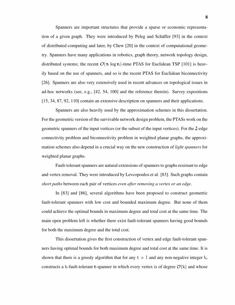
Spanners are important structures that provide a sparse or economic representa-

tion of a given graph. They were introduced by Peleg and Schaffer [93] in the context

of distributed computing and later, by Chew [20] in the context of computational geome-

try. Spanners have many applications in robotics, graph theory, network topology design,

distributed systems; the recentb log -time PTAS for Euclidean TSP [101] is heav-

ily based on the use of spanners, and so is the recent PTAS for Euclidean biconnectivity

[26]. Spanners are also very extensively used in recent advances on topological issues in

ad-hoc networks (see, e.g., [42, 54, 100] and the reference therein). Survey expositions

[15, 34, 87, 92, 110] contain an extensive description on spanners and their applications.

Spanners are also heavily used by the approximation schemes in this dissertation.

For the geometric version of the survivable network design problem, the PTASs work on the

geometric spanners of the input vertices (or the subset of the input vertices). For the -edge

connectivity problem and biconnectivity problem in weighted planar graphs, the approxi-

mation schemes also depend in a crucial way on the new construction of light spanners for

weighted planar graphs.

Fault-tolerant spanners are natural extensions of spanners to graphs resistant to edge

and vertex removal. They were introduced by Levcopoulos et al. [83]. Such graphs contain

short paths between each pair of vertices even after removing a vertex or an edge.

In [83] and [86], several algorithms have been proposed to construct geometric

fault-tolerant spanners with low cost and bounded maximum degree. But none of them

could achieve the optimal bounds in maximum degree and total cost at the same time. The

main open problem left is whether there exist fault-tolerant spanners having good bounds

for both the maximum degree and the total cost.

This dissertation gives the first construction of vertex and edge fault-tolerant span-

ners having optimal bounds for both maximum degree and total cost at the same time. It is

shown that there is a greedy algorithm that for any v 3and any non-negative integer = ,

constructs a = -fault-tolerant -spanner in which every vertex is of degreeD = and whose

9

total cost isD = 1 times the cost of minimum spanning tree; these bounds are asymp-

totically optimal. An efficient algorithm is designed to find fault-tolerant spanners with

asymptotically optimal bound for the maximum degree and almost optimal bound for the

total cost based on a new, sufficient condition for a graph to be a = -fault-tolerant spanner.

1.3 Outline

The dissertation contains two parts. Part I is dedicated to scheduling problems in master-

slave systems. The new results are joint work with J. Leung which appear in [79, 80].

These results are presented in three chapters. In Chapter 2, the master slave model and

some of its applications are first introduced. Then the problems going to be studied are

defined. Finally the new complexity results are presented. The complexity results show

that many makespan and total completion time problems, with or without constraints, are

NP-hard in the strong sense. Thus the following two chapters concentrate on approximation

algorithms.

Chapter 3 considers special cases of the problems in master slave model, which

assume that (1) there is a single master, (2) all jobs have the same release time 9 , same

preprocessing task length and same postprocessing task length U ; i.e. the jobs are different

from each other only by their slave tasks, (3) no preemption is allowed. First it is proved

that if there are canonical and order preserving constraints, then in ¤ log time one

can find an optimal schedule that minimizes the total completion time, when J¥ and

UL¥ U for all3z§¦( and U . After that, approximation algorithms are developed

for the canonical total completion time problem and the no-wait-in makespan problem,

respectively.

Chapter 4 considers the general cases of total completion time problem. Efficient

approximation algorithms are developed to minimize the total completion time in various

settings. These are the first general results for the total completion time problem in the

10

master-slave model. Furthermore, these algorithms are shown to generate schedules with

small makespan as well.

The second part of this dissertation is dedicated to network design problems. In

Chapter 5, the PTASs for the geometric version of the survivability problems are presented.

This include the first PTAS for the Steiner tree problem, the 8<9 3" "; -connectivity problem

and the multigraph variant 8:9 3" ''' =; -edge connectivity problem. The results of this

chapter have been published in [27] and they are joint work with A. Czumaj and A. Lingas.

Chapters 6 and 7 consider the -connectivity problem and its variations in planar

graphs. In Chapter 6, the PTASs for the -edge-connectivity and biconnectivity problem in

unweighted planar graphs are described. Chapter 7 discusses the weighted planar graphs.

First a PTAS is presented for the problem of finding minimum-weight 2-edge-connected

spanning subgraphs where duplicate edges are allowed. Then a new greedy spanner con-

struction for edge-weighted planar graphs are given. This construction augments any con-

nected subgraph ¨ of a weighted planar graph

to a:3x u -spanner of

with total weight

bounded by weight ¨ u . Based on this spanner, quasi-polynomial time approximation

schemes are derived for the problems of finding the minimum-weight 2-edge-connected

or biconnected spanning subgraph in planar graphs. Approximation schemes are also de-

signed for the minimum-weight 1-2-connectivity problem, which is the variant of the sur-

vivable network design problem where vertices have non-uniform (1 or 2) connectivity

constraints. Chapter 6 contains joint work with A. Czumaj, M. Grigni, P. Sissokho, and ap-

pears in [24]. Chapter 7 contains joint work with A. Berger, A. Czumaj and M. Grigni in

[9].

Chapter 8 presents two new results about vertex and edge fault-tolerant spanners in

Euclidean spaces. First it is shown that a greedy algorithm that for any ©v 3 and any non-

negative integer = , constructs a = -fault-tolerant -spanner in which every vertex is of degreeb = and whose total cost isD = 1 times the cost of minimum spanning tree; these bounds

are asymptotically optimal. The next contribution is an efficient algorithm for constructing

11

good fault-tolerant spanners. A new, sufficient condition for a graph to be a = -fault-tolerant

spanner is developed. Using this condition, one can design an efficient algorithm that finds

fault-tolerant spanners with asymptotically optimal bound for the maximum degree and

almost optimal bound for the total cost.

Finally, Chapter 9 summarizes the contributions of the dissertation. Some possible

extensions and future research directions are also remarked.

PART I

SCHEDULING PROBLEMS INMASTER-SLAVE MODEL

12

CHAPTER 2

COMPLEXITY OF SCHEDULING PROBLEMS IN MASTER-SLAVE MODEL

2.1 Master-slave Model

The master-slave model was recently introduced by Sahni [104]. In this model, each job

has to be processed sequentially in three stages. In the first stage, the preprocessing task

runs on a master machine; in the second stage, the slave task runs on a dedicated slave

machine; and in the last stage, the postprocessing task again runs on a master machine,

possibly different from the master machine in the first stage. The preprocessing, slave and

postprocessing tasks and task times of job¦

are denoted by J¥ , ª¥ and U^¥ , respectively. It is

assumed that ¥-v«9 , ª¥-v«9 and U^¥Av9 .A job may have a release time ¥5§9 , i.e., ¥ cannot start until ¥ . Without loss of

generality, one can assume that min L, 9 . Unless stated otherwise, all jobs are assumed to

have the same release time. There are two cases when arbitrary release time is present. The

first case deals with offline problems, i.e., the release times and processing times of all jobs

are known in advance. The second case deals with online problems, i.e., no information of

a job¦

is given until it arrives at ¥ , and when it arrives, all parameters about job¦

is given.

The quadruple ¥ ¥ ª¥ U^¥ is used to denote job

¦. For simplicity, if ¥ 9 , one can use

the triplet ¥ ª¥ U^¥ to represent job

¦.

Each machine is either a master machine or a slave machine. The master machines

are used to run preprocessing and/or postprocessing tasks, and the slave machines are used

to run slave tasks, one slave machine for each slave task. In a single-master system, there

is a single master to execute all preprocessing tasks ( tasks) and postprocessing tasks

( U tasks). In a multi-master system, there are more than one master, each of which is

capable of processing both tasks and U tasks. Finally, in some systems, there are distinct

13

14

preprocessing masters (preprocessors) and postprocessing masters (postprocessors), which

are dedicated to process tasks and U tasks, respectively.

The master-slave model is closely related to the flow shop model. The system

which has a single preprocessor and a single postprocessor can be seen as a two-machine

flow shop with transfer lags. In this flow shop model, each job | has two operations: the

first operation is scheduled on the upstream machine and the second operation is scheduled

on the downstream machine. The interval or time lag between the finish time of the first

operation and the start time of the second operation must be exactly or at least , . If the :, ’sare large enough such that all of the first operations finish before the start of any second

operation, then the flow shop problem is equivalent to the problem of scheduling on a single

machine with time lags and two tasks per job, subject to the constraint that all of the first

operations are scheduled first. The latter problem is identical to the single-master master-

slave scheduling model.

When there are more than one preprocessing and postprocessing masters, the master-

slave model can be seen as a two-stage hybrid flow shop with transfer lags. In this sense,

the single master case can be regarded as a three-stage hybrid flow shop where the first and

the last stage has a single machine and the second stage has machines. Hybrid flow shop

is often found in electronic manufacturing environment such as IC packaging and make-

to-stock wafer manufacturing. In recent years, hybrid flow shop has received significant

attention, see [12], [75], [78] and [112].

2.2 Applications of Master-slave Model

The master-slave model finds many applications in parallel computer scheduling and in-

dustrial settings such as semiconductor testing, machine scheduling, transportation main-

tenance, etc. Some of them are listed in the following. For more applications, see [104],

[106], [105] and [115].

15

Several applications of the master-slave model are found in parallel computer schedul-

ing. A common parallel programming paradigm involves the use of a main computational

thread whose function is to prepare data then fork and initiate new child threads that do the

computations on different processors. After the computation of a child thread, the main

thread collects the computation results and performs some processing on the results. Here,

each child thread can be seen as a job with three tasks: the thread initiation and data prepa-

ration is the preprocessing task, the computation is the slave task and the postprocessing of

the results from the computation is the postprocessing task.

The master-slave paradigm also has applications in certain semiconductor testing

operations. In the case of burn-in operations, chips are subject to thermal stress for an

extended period of time. The whole process for each chip consists of three phases. First, an

initial burn-in operation is accomplished by maintaining the oven at a constant temperature

while powering up the chip. The burn-in times for each chip are specified by the customer

and thus fixed a priori. Then, in the second phase, the chip cools off for a specified amount

of time that depends on the length and intensity of the initial burn-in period. In the last

phase, the chip is subject to a final burn-in operation. In this application the burn-in oven

corresponds to the master machine, the two burn-in tasks correspond to preprocessing and

postprocessing and the cooling period corresponds to the slave task. Since the burn-in

operations are near the end of the production process, scheduling is critical in determining

on-time delivery and output performance for the entire company.

Industrial applications of the master-slave paradigm include the case of consolida-

tors that receive orders to manufacture quantities of various items. The actual manufac-

turing is done by a collection of slave agencies. In this example, the consolidator is the

master machine and the slave agencies are the slave machines. The consolidator needs to

assemble the raw material needed for each task, load the trucks that will deliver this mate-

rial to the slave machines, and perform an inspection before the consignment leaves. All of

these work belong to preprocessing task. The slave machines need to wait for the arrival of

16

the raw material, inspect the received goods, perform the manufacture, load the goods on-

to the trucks for delivery, perform an inspection as the trucks are leaving. These activities

together with the delay involved in getting the trucks to their destination (i.e., the consol-

idator) represent the slave work. When the finished goods arrive at the consolidator, they

are inspected and inventoried. This represents the postprocessing.

It is easy to see that all of the above examples generalize to multi-master systems

or distinct preprocessing and postprocessing master systems.

2.3 Scheduling Problems in Master-slave Model: Definitions and Notations

Given a set of jobs in the master-slave system and a scheduleX

of the jobs, two jobs¦and | are said to overlap in

Xif the master machine is working on the preprocess-

ing/postprocessing task of job¦

while a slave machine is working on the slave task of

job | . Note that there may be several jobs overlapping with a given job¦.

The completion (or finish) time of job¦

in a scheduleX

is the time when the post-

processing task U^¥ finishes. The completion time of¦

inX

is denoted by +[¥ X . IfX

is clear

from the context, +-¥ , instead of +¥ X , is used. The makespan ofX

is the earliest time when

all the tasks have been completed. The makespan ofX

is denoted by + max X

, or + max ifX

is clear from the context. The total completion time ofX

, denoted by + X , is the sum of

the completion times of all jobs, i.e., + X *¬,®/ +-, X .Makespan and total completion time are two common objectives to minimize. The

problems of finding a schedule that minimizes the makespan and total completion time are

referred to as the makespan ( + max) problem and total completion time ( * +-, ) problem, re-

spectively. A schedule that minimizes + max or * +, is usually denoted byX T . Throughout

this dissertation, + Tmax and + T are used to denote the minimum makespan and the minimum

total completion time, respectively.

A non-preemptive schedule is one that schedules each task without interruption.

Note that in such a schedule, it is still possible that there is an interval between the finish

17

time of ¥ and the start time of ª¥ , or the finish time of ª¯¥ and the start time of U°¥ . How-

ever, without loss of generality, one can always assume that ª¥ is scheduled immediately

as soon as ¥ completes. In a preemptive schedule, a job running on one machine may be

interrupted for some time, and later resumed on possibly a different machine. Both non-

preemptive and preemptive schedules have some applications. In the consolidators exam-

ple, non-preemptive schedules are more realistic than preemptive schedules. On the other

hand, in the parallel computer scheduling example, preemptive schedules are as realistic as

non-preemptive schedules.

A non-preemptive scheduleX

is order preserving if for any two jobs¦

and | such

that ¥ completes before , , U^¥ must also complete before U±, . A no-wait-in schedule is one

such that each slave task must be scheduled immediately after the corresponding prepro-

cessing task finishes and each postprocessing task must be scheduled immediately after the

corresponding slave task finishes. In other words, once a job starts, it will not stop until it

finishes. It is easy to see that a no-wait-in schedule must be non-preemptive.

A canonical schedule on the single master system is one such that all the prepro-

cessing tasks complete before any postprocessing tasks can start (Note that the definition

of canonical schedule is slightly different from the one given in [104]). In the multi-master

system, a canonical schedule is one that is canonical on each master. Both canonical and

non-canonical schedules have some applications. In the consolidators example, canonical

schedules make sense while non-canonical schedules do not. On the other hand, in the par-

allel computer scheduling example, non-canonical schedules make sense while canonical

schedules do not.

It is easy to see that if all jobs have the same release time, one can always arrange a

schedule to be canonical without increasing the makespan. Thus, in order to minimize the

makespan in this case, one only needs to focus on canonical schedules. However, this is

not true if one wants to minimize * +, . In fact, the ratio of the total completion time of the

best canonical schedule versus that of the best non-canonical schedule can be arbitrarily

18

large. Consider the example: ²N 3 identical jobs

:3" u 3 and one job 1 u 3 , where u

is an arbitrary small positive number. The optimal canonical schedule has total completion

time ¤ ´³ , while the optimal non-canonical schedule has total completion time ¤ 1 .

2.4 Previous Work

So far the main research efforts to the master-slave model are for makespan minimization,

assuming all jobs have the same release time. As noted before, it is sufficient to focus on

canonical schedules for the makespan objective in this case. The general makespan problem

without constraints has been shown to be NP-hard by Kern and Nawijn [69]. Sahni [104]

showed that the no-wait-in makespan problem is NP-hard in the ordinary sense, even when

there is order preserving constraint. He also gave an ¤ log -time algorithm that solves

the order preserving makespan problem.

Sahni and Vairaktarakis [106] proposed several constant approximation algorithms

for the makespan problem in the single-master and multi-master systems. For the general

problem without any constraints, they gave a ³1 -approximation algorithms for the single

master system and a -approximation algorithms for the multi-master systems.

Further algorithms were given by Vairaktarakis [115] when there are .C/ preproces-

sors and .21 postprocessors. Let . max8<.0/ .D1; . He gave approximation algorithms

with a worst-case bound of N /µ for the makespan problems with no constraint, or with

the constraints of order preserving.

Flow shop is a classical model that has been studied for a long time. Let . be the

number of stages. For the makespan problem, Johnson [65] developed an ¤ log time

optimal algorithm when . . The problem becomes NP-hard when .5¶ . In this case,

Hall [58] presented a<3&x u -approximation algorithm for any fixed positive u . For the total

completion time problem, it is NP-hard in the strong sense even if . and preemption

is allowed [33]. Gonzalez and Sahni [46] developed an approximation algorithm for this

problem in the . -stage flow shop model. The approximation ratio of their algorithms is

19

. . Let ·W¥ be the total processing time of all operations of job¦. The algorithm schedules

the jobs in nondecreasing order of ·K¥ at each stage. By a careful analysis, Hoogeveen et

al. [61] showed that this algorithm has approximation ratio ¸¯ n x ¸ , where n denotes

the minimal processing time of all tasks and ¸ denotes the maximal processing time of all

tasks. If the jobs have different weights, Schulz [108] obtained an approximation algorithm

with performance guarantee of . (or . xE3in case of arbitrary release time) for total

weighted completion time based on linear programming.

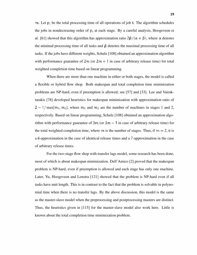
When there are more than one machine in either or both stages, the model is called

a flexible or hybrid flow shop. Both makespan and total completion time minimization

problems are NP-hard, even if preemption is allowed; see [57] and [33]. Lee and Vairak-

tarakis [78] developed heuristics for makespan minimization with approximation ratio of

N 3 max8:.0/ .D1P; , where .¹/ and .D1 are the number of machines in stages 1 and 2,

respectively. Based on linear programming, Schulz [108] obtained an approximation algo-

rithm with performance guarantee of ¶º. (or ¶º. x»3in case of arbitrary release time) for

the total weighted completion time, where . is the number of stages. Thus, if . , it is

a ¼ -approximation in the case of identical release times and a ½ -approximation in the case

of arbitrary release times.

For the two-stage flow shop with transfer lags model, some research has been done,

most of which is about makespan minimization. Dell’Amico [2] proved that the makespan

problem is NP-hard, even if preemption is allowed and each stage has only one machine.

Later, Yu, Hoogeveen and Lenstra [121] showed that the problem is NP-hard even if all

tasks have unit length. This is in contrast to the fact that the problem is solvable in polyno-

mial time when there is no transfer lags. By the above discussion, this model is the same

as the master-slave model when the preprocessing and postprocessing masters are distinct.

Thus, the heuristics given in [115] for the master-slave model also work here. Little is

known about the total completion time minimization problem.

20

2.5 New Results: Complexity of Scheduling Problems in Master-slave Model

First, some previous complexity results for the makespan problem is strengthened. Then

some new results for the total completion time problem are developed, based on the re-

sult from [121]. It is shown that many problems are strongly NP-hard, even with some

constraints. The main results can be summarized as follows:

The makespan problem is strongly NP-hard, even if &¥ U^¥ ¾3for

3¿À¦7 and

only no-wait-in schedules are considered.

The order preserving and no-wait-in makespan problem is NP-hard in the strong

sense, even if ¥ U^¥ for all3(«¦ .

The total completion time problem is NP-hard in the strong sense, even if (i) all the

preprocessing and postprocessing tasks have unit time, (ii) only canonical, or no-

wait-in, or canonical and no-wait-in schedules are considered.

The order preserving and no-wait-in total completion time problem is NP-hard in the

strong sense, even if ¥ UL¥ for all3(«¦H .

It is sufficient to prove the above results in the simple case: a single master and

all jobs have the same release time. Following is a theorem about + max problem in a two-

machine flow shop with delays which was recently proved by Yu et al. [121].

Theorem 2.5.1 (See Theorem 21 and Corollary 22 [121]) The flow shop problem Á° , ·W¥Â, 3 Ã+ max is strongly NP-hard, even if exact delays are required.

By the discussion in Section 2.1, the above theorem immediately implies the fol-

lowing theorem.

Theorem 2.5.2 The makespan problem in master slave system with J¥ U^¥ Ä3for all3£¦H is strongly NP-hard, even if there is no-wait-in constraint.

21

Proof : The outline of the proof of this theorem is given below, as it is relevant to the

discussion of the total completion time problem later. The reduction is almost the same

as in the proof of Theorem 21 in [121]. But for each job¦, instead of having a lag ~¥

between its two tasks, it now has a slave task ªÅ¥ which must start after the preprocessing

task and finish before the postprocessing task. The preprocessing and postprocessing tasks

are performed on the same master machine, instead of two machines. To ensure the same

argument goes through, let ª¯¥ i¥ xzÆ for each job¦, where

ÆÇ gN .È x and is the

number of jobs in the instance of the two-machine flow shop with delays. The bound for

the makespan is also increased byÆ

. The proof of Theorem 21 in [121] used a reduction

from the ¶ -partition problem, which is known to be strongly NP-complete; see [43].

A ¶ -partition problem instance has input as a set of non-negative integers É 8ËÊ/ Ê1 ''' , Ê ³ µ ; and a non-negative integer È such that * ³ µ¥Ì/ Êº¥ .È and ÈÍ^ÎtÏlÊº¥[ÏÈÍ° for all

3yÐ¦Ñ ¶º. . The problem is to decide whether É can be partitioned into .disjoint subsets É/ , ..., É µ such that for all

3 | . , *ÒÓÕÔÖ±×°Ê¥ È ? In the following

É-, is used to denote a partition subset, where3( | . .

An instance of the makespan problem can be constructed as follows. There are

. 1 È x .È jobs. For job¦,3¦Ø ¶º. , referred to as a

O-job in [121], ªÅ¥ Êº¥ xÙÆ

whereÆÙ 0N .È x ; for job

¦, ¶º. x»3m¦£ .È , referred to as a Ú -job in [121],

ªJ¥ ÛÆ, and for job

¦, .È x¾3«Ü¦ . 1 È x .¹È , referred to as an Ý -job in [121],

ªJ¥ Þ . x»3 È xl3xCÆ . For all job¦,3g»¦$ , let ¥ U^¥ ¾3

. Let the bound for the

makespan be .È x x xÙÆß à .

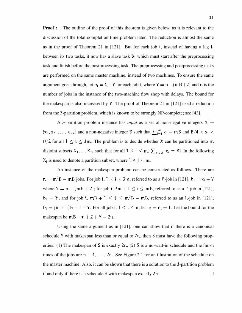
Using the same argument as in [121], one can show that if there is a canonical

scheduleX

with makespan less than or equal to à , thenX

must have the following prop-

erties: (1) The makespan ofX

is exactly à , (2)X

is a no-wait-in schedule and the finish

times of the jobs are xl3 , ''' , à . See Figure 2.1 for an illustration of the schedule on

the master machine. Also, it can be shown that there is a solution to the ¶ -partition problem

if and only if there is a scheduleX

with makespan exactly à . á

22

kP1jP

1iP2iP1k

P1jP

1iP

1ZZZZ ZLLLLZLLLLZL ZZ ZZLL L Z Z

2iP −1mB

(b)

Z

postprocessing tasks of n jobspreprocessing tasks of n jobs

mB

n+(mB+2)(mB+2)

Z

(a)

0 n

mBmB

mB

kP1i

P −1

−11kP−1

1jP

2iPZ

1

−11kP−1

1jP

1iP −1

mB2i

P −1−11jP −1

ZL

2M

1M2iP

1kP

1jP

1iP L

−11kP−1

1jP

1iP −1

LLZL ZZ ZZLL L Z

M

2iPZ ZZZZ

1iP −1

Z iP 1 ZLLLL1kP

1jP

Figure 2.1 (a) An illustration of the schedule that minimizes the makespan for the problem in-stance in the two-machine flow shop model with lags reduced from â -partition in [121], (b) Anillustration of the schedule on the master machine that minimizes the makespan problem instancereduced from â -partition in Theorem 2.5.2.

The above result can be used to show that the total completion time problem is also

strongly NP-hard.

Theorem 2.5.3 The total completion time problem with &¥ U^¥ 3for all

3l¦7 is

strongly NP-hard, even if (1) only canonical schedules are considered, or (2) only no-wait-

in schedules are considered, or (3) canonical and no-waited-in schedules are considered.

Proof : The reduction is still almost the same as above, the only difference is that now

one asks the question: is there a schedule of the tasks with total completion time at most

1 x ¬ãä¬å /<æ1 ?

It is sufficient to prove that there is a schedule with total completion time less than

or equal to 1 x ¬&ã ¬"å /<æ1 if and only if there is a schedule with makespan less than or equal

to à .

“If” part. LetX

be a schedule with makespan less than or equal to .È x xÆ N¿ à . By the proof of Theorem 2.5.2,

Xmust be a canonical and no-wait-in schedule and the

completion time of the jobs are x3 , x , ''' , à . Thus the total completion time is

exactly 1 x ¬&ã ¬"å /<æ1 .

“Only if” part. LetX T be a schedule for the jobs constructed above such that

* +, X T ( 1 x ¬&ã ¬"å /<æ1 . For any job¦,32¦z , let +Hç Ó X T denote the time when

23

the task ¥ finishes in the scheduleX T . Then, +Hç Ó X T 5 3

, and if¦yj | then +Hç Ó X T mj

+6ç × X T . Thus * ¬ ¥Ì&/ +6ç Ó X T 5 <3Hx x»èèè^x [ /1 xl3 . Since +¥é5¾+6ç Ó X T ÅxªJ¥ x U^¥ +6ç Ó X T Jx ª¥ x3 , the following inequality holds.

¬ê¥Ì/ +A¥

X T 5 ¬ê¥Ì&/ +6ç Ó X T Jx ªJ¥ xÀ3A ¬ê

¥Ì&/ +6ç Ó X T Jx ¬ê

¥ë/ ª¥x À5 3

x»3Jx ¬ê¥Ì/ ª¥

x ì'Note that *À¬¥Ì/ ª¥ Æ0x * ³ µ¥Ì/ Ê¥ x . 1 È . xí3 È x3b 1 N» . This means

that *À¬¥Ì&/ +A¥ X T 5 1 x ¬&ã ¬"å /îæ1 . By the assumption aboutX T , it must be true that

* ¬ ¥Ì/ +A¥ X T 6 1 x ¬ãä¬å /<æ1 . ThusX T must be a canonical and no-wait-in schedule. Fur-

thermore, the completion time of the jobs must be x3 , x , ''' , à . Thus the makespan

of the schedule is à .

This completes the proof. áThe above theorem implies that the total completion time problem is NP-hard in

the strong sense even if preemption is allowed. Observe that the optimal scheduleX

for the

constructed instance in the proof of Theorem 2.5.2 is not order preserving, so the above

results are not applicable to order preserving scheduling problems. In the following, the

complexity of no-wait-in makespan and no-wait-in total completion time problem with the

constraint of order preserving will be considered. Both problems will be shown to be NP-

hard in the strong sense by a reduction from the ¶ -partition problem.

Theorem 2.5.4 The problem of minimizing the order preserving and no-wait-in makespan

is strongly NP-hard, even if ¥ U^¥ for3)«¦H .

Proof : To reduce an instance of ¶ -partition problem to an instance of the scheduling

problem, one first create two types of jobs. This include (1) ¶º. partition jobs: J¥ U^¥ Ê¥and ª¥ ¶È x ¿NÊº¥ , 3tE¦ ¶º. , and (2) . separation jobs: ¥ UL¥ È x§3 and

ªJ¥ È , ¶º. x3Ü¦ðï . . The problem is to determine whether there is an order

preserving and no-wait-in-schedule such that + max . ¶È x . Clearly, the reduction

can be done in polynomial time.

24

B+1 2B+10 3B+2 4B+3 5B+3 6B+4 2m(3B+2)

c1 c2 c3a3m+1 a3a2a1

a3m+2 c3m+2c3m+1M

Figure 2.2 An illustration of the schedule on the master machine for the instance reduced from â -partition in Theorem 2.5.4. Jobs h , ñ and â are partition jobs, jobs âò0ózh and âò¹ó(ñ are separationjobs.

If there is a solution to the ¶ -partition problem, then one can schedule the separation

jobs in any order without overlapping, and for each group of ¶ -partition jobs corresponding

to a partition subset, schedule their preprocessing tasks fully overlapping with the slave task

of one separation job and the postprocessing tasks fully overlapping with slave task of the

separation job immediately following the previous one. See Figure 2.2 for an illustration

of the schedule. It is clear that the schedule is order preserving and no-wait-in and + max

. ¶È x . Now suppose the scheduling problem has a solution; i.e., there is an order

preserving and no-wait-in scheduleX

such that + max . ¶È x . Since only no-wait-

in schedules are considered and since ¥ U^¥6v§ª¯, for any two separation jobs¦

and | , a

separation job can not overlap with another one. Hence, + max 5*»ô µ,® ³ µ å / , x ª¯, x U°, A. ¶È x . By assumption, + max . ¶È x . Therefore + max

. ¶È x ,which means that all the partition jobs must fully overlap with the separation jobs. For

each partition job¦, È¹Ï§ª¯¥Ï¶È x . Therefore, each partition job

¦must overlap with

exactly two adjacent separation jobs in the scheduleX

. Because ÈÍ^ÎÏõJ¥ U^¥HÏöÈÍ° ,at most three preprocessing and/or postprocessing tasks of the partition jobs overlap with

one separation job. Since there are . separation jobs only, there must be exactly three

preprocessing or postprocessing tasks fully overlapping with each separation job. For each

separation job | , ªÅ, È . Thus, the integers corresponding to the three preprocessing or

postprocessing tasks that overlap with ªW, have a total exactly È . Hence, the ¶ -partition

problem has a solution. áTheorem 2.5.5 The problem of minimizing the order preserving and no-wait-in total com-

pletion time is strongly NP-hard, even if ¥ U^¥ for3)«¦H .

25

÷²÷÷²÷÷²÷÷²÷øøøø (2m+2l)(3B+2)+l ε4B+3 5B+3 6B+4 2m(3B+2)3B+22B+1B+1 (2m+1)(3B+2)0 (2m+2)(3B+2)+

a1a 1c3c2ca

ε

c5m+1a5m+1c3m+2a3m+2c3m+1a3m+1 2 3

Figure 2.3 An illustration of the schedule on the master machine for the instance reduced from â -partition in Theorem 2.5.5. Jobs h , ñ and â are partition jobs, jobs âò§óh and âò§óyñ are mediumjobs and job ùLòúóh is a large job.

Proof : As in the previous proof, the reduction is from ¶ -partition problem. First three

types of jobs are created for the scheduling problem: (1) ¶º. small jobs: J¥ U^¥ Ê¥ and

ªJ¥ ¶È x gNûÊº¥ , 3ßw¦z ¶º. ; (2) . medium jobs: ¥ UL¥ È xE3 and ª¥ È ,

¶º. x3£«¦«ï . ; (3) large jobs: ¥ UL¥ ¶È x and ª¥ u , ï . x3(«¦«ï . x , uis a small positive number and is an integer greater than ¶º¼. 1 x²3ü . x àÎ. 1 È x²3 .È .

Let

È-ý ¶È x Åè . . x»3DÈÍþ . ¶È x &x x»3 ¶È x &x 3

xÀ3 u and

ÈKÿ ¶º. B¶º.È x . x ½Î È xÀ3 'Let ÈÍT ÈKÿ x È-ý x ÈÍþ . The scheduling problem is: Is there an order preserving and

no-wait-in schedule of these jobs such that * ô µ å,®/ +-, ÈÍT ?

If the partition problem has a solution, then schedule the jobs as follows: first sched-

ule the medium jobs in any order without overlapping; schedule any three small jobs that

correspond to the three integers in the same partition subset fully overlapping with two ad-

jacent medium jobs; finally, schedule the large jobs after the medium jobs one by one in

any order without overlapping. See Figure 2.3 for an illustration of the schedule. One can

easily verify that the schedule is an order preserving and no-wait-in schedule. To bound

the total completion time, the total completion time of each type of jobs is calculated sepa-

rately. Without loss of generality, suppose that the medium jobs are scheduled in the order

of ¶º. x3, ¶º. x , ''' ,

ï . . Since the medium jobs are scheduled one by one from time

26

9 without overlap, the total completion time of all medium jobs is

ô µê¥Ì ³ µ å /

d¦ N¹¶º. Wè ¥ x ªJ¥ x U^¥ K 1 µê¥Ì/

¦-è ¶È x K ¶È x Wè . . x3Í È-ý 'Similarly, the total completion time of all large jobs is

ô µ åê¥ë ô µ å /

. ¶È x &x§Ì¦ N ï . Wè ¥ x ª¥ x U^¥ è . ¶È x Jx ê

¥ë/¦^ ¶È x Jx u

. ¶È x &x x3 ¶È x Jx 3 x3 u ÈÍþû'

Now consider the total completion time of the small jobs. Suppose that the small

jobs corresponding to the partition subset É´, , 3D | . , are | / , |Ë1 and | ³ ; furthermore,

suppose that | / is scheduled before |i1 which is scheduled before | ³ . Suppose that these jobs

overlap with two consecutive medium jobs ¶º. x "|ÅN 3 and ¶º. x "| . Let +´, Ó denote the

completion time of the small job |i¥ . Then

+, |N 3 ¶È x Jx§ È x»3x , x ª¯, x U^, |N 3 ¶È x Jx§ È x»3x Ê, x ¶È x 7N0Ê, x Ê, Ì "|N 3 ¶È x Jx§ È x»3x Ê, Ï Ì "|N 3 ¶È x Jx§ È x»3x 3

Èõ'Similarly, one can get

+, |N 3 ¶È x x È x»3&x , &x , x ª¯, x U°, |N 3 ¶È x x È x»3&x Ê, &x Ê, xú ¶È x ©N0Ê, Jx Ê, Ì "|N 3 ¶È x x È x»3x Ê, x Ê, Ï Ì "|N 3 ¶È x x È x»3x ¶Î È

and

+, |JN 3 ¶È x Jx È xÀ3Jx , x , &x , x ª¯, x U°,

27

|JN 3 ¶È x Jx È xÀ3Jx Ê, x Ê, &x Ê, xú ¶È x £N¹Ê, &x Ê, d "|JN 3 ¶È x Jx È xÀ3x Ê, x Ê, x Ê,d "|JN 3 ¶È x Jx È xÀ3x Èõ'

Thus,

+, x +, x +-, ÏÀ¶ èÌ "|&N 3 ¶È x &xú È x»3x 3 È x ¶Î È x È ¶ èÌ "|&N 3 ¶È x &xú È x»3x üÎ Èõ'

Hence, the total completion time of all small jobs is

³ µê,®/ +,

µê,®/

³ê¥Ì&/ +, Ó Ï

µê,®/ ¶ è "|N 3 ¶È x x È x»3&x üÎ È ¶º. 1 è ¶È x &x ¶º. È x»3&x üÎ .È ¶º. ¶º.È x . x ½Î È x3 ÈKÿÀ'

Therefore, the total completion time of all jobs is

³ µê,®/ +,

x ô µê, ³ µ å /

+, x ô µ åê,® ô µ å /

+,ÅÏÈKÿ x È-ý x ÈÍþ È T 'Now, suppose there is an order preserving and no-wait-in schedule of all these jobs

such that * ô µ å,®/ +, È T . One need to show that there is a solution to the partition prob-

lem. LetX T be such a schedule with the smallest total completion time. Some observations

aboutX T are listed as follows.

First, , U^,)v ª¥ for any two jobs¦

and | that are both medium jobs or large

jobs. Therefore,¦

and | can not overlap with each other inX T . For the same reason, a large

job can not overlap with a medium job inX T , nor can it overlap with a small job. Hence,

overlapping can only occur between the small jobs or between the small and medium jobs.

Next, because ¥ UL¥ Ê¥©v ÈÍ^Î for any small job¦,3D¦ ¶º. , there are at most

three small preprocessing/postprocessing tasks that can overlap with the slave task ªÍ, of a

28

medium job | . Since ÈÏÀª¯¥Ïû¶È x for any small job¦, ª¯¥ can overlap with tasks of at

most two medium jobs in the scheduleX T .

Finally, there are two other properties ofX T .

Large jobs are scheduled after all medium jobs finish inX T .

As shown above, the large jobs can not overlap with the medium jobs and small jobs.

Suppose that some medium jobs and small jobs are scheduled between two large

jobs. Then one can modify the schedule by moving the first large job so that it is

scheduled immediately before the second large job. Since no small or medium jobs

can overlap with the large jobs, this movement will not affect the feasibility of the

schedule, i.e., it is still an order preserving and no-wait-in schedule. However, the

new schedule has a smaller total completion time which contradicts the assumption

thatX T is optimal.

Exactly three small jobs overlap with a medium job inX T .

It is clear that a small job can not be scheduled after a large job; otherwise, one can

interchange them without increasing the total completion time. Similarly, a small job

can not be scheduled between two medium jobs. Therefore, a small job can only be

scheduled either before all medium and large jobs or fully overlapping with medium

jobs.

Suppose there is a preprocessing task &¥ of a small job¦

which is scheduled before

any medium or large jobs inX T . Then,

ô µ åê¥Ì&/ +A¥

X T v ô µ åê, ³ µ å /

+, X T

5 ô µê, ³ µ å /

¥ x |NÙ¶º. Wè , x ª, x U°, x ô µ åê

,® ô µ å / ¥ x . ¶È x Jx§ |N ï . Wè , x ª, x U°,

29

. x ¥ x 1 µê ,®&/ | è ¶È x x :. ¶È x &x ê

,®/ |è ¶È x x u

. x ¥ xû¡ x Ýv 3Î . x È x È T NûÈKÿ'

By assumption, vÀ¶º¼. 1 x»3ü . x àÎ. 1 È xl3 .ÇÈ . Thus, ÈÍÿ(Ï / . x È .

Hence, * ô µ å¥Ì&/ +A¥ X T vÀÈÍT , contradicting the assumption that * ô µ å¥Ì&/ +¥ X T [ ÈÍT .Therefore, every small job must overlap with exactly two adjacent medium jobs inX T . Since there are . medium jobs and ¶º. small jobs, there must be exactly three

preprocessing tasks or three postprocessing tasks overlapping with a medium job.

For any medium job | , there are exactly three small jobs overlapping with it inX T .

Because ª¯, È , the sum of the preprocessing or postprocessing tasks of the three small

jobs overlapping with | is exactly È , which means that the corresponding three integers

have a total exactly È . Thus, the partition problem has a solution.

á

CHAPTER 3

OPTIMAL AND APPROXIMATION ALGORITHMS: SPECIAL CASES

This chapter considers special cases of the total completion time minimization problem and

no-wait-in-makespan problem. It is assumed that (1) there is a single master, (2) all jobs

have the same release time 9 , same preprocessing task length and same postprocessing

task length U ; i.e., the jobs are different from each other only by their slave tasks, (3) no

preemption is allowed. It is proved that in this case if there are canonical and order preserv-

ing constraints, then in ¤ log time one can find an optimal schedule that minimizes

the total completion time, when ¥ and U^¥ U for all34¦¿ and U . After

that, some approximation algorithms are developed for the canonical total completion time

problem and the no-wait-in makespan problem.

3.1 Optimal Algorithms for * +, : Canonical and Order Preserving Schedules

It has been shown in Chapter 2 that minimizing total completion time is strongly NP-hard,

even under severe constraints. This section shows that there is a special case that admits a

polynomial time algorithm.

Theorem 3.1.1 The problem of minimizing the canonical and order preserving total com-

pletion time can be solved in ¤ log time if ¥ and U^¥ U for3D¦ and

U .Proof : The proof is by showing that a canonical schedule

X T that schedules the pre-

processing tasks in nondecreasing order of the processing times of the slave tasks gives an

optimal order preserving schedule.

For any job¦, let W¥ denote the rank of job

¦inX T ; i.e., ¥ is the W¥ -th task scheduled

inX T . Because only canonical schedules are considered, the earliest possible time to start

30

31

UL¥ is ¥ max 7 W¥ x ª¥ . For any two jobs

¦and | , if ¥7ÏW, and ª¥ ª¯, , then

¥ , . By the definition of canonical schedules, Uà¥ will be scheduled before Uà, . Thus,X T

is order preserving.

The next step is to show thatX T has the minimum total completion time among all

canonical and order preserving schedules. Suppose there is another canonical and order

preserving scheduleX

that is optimal. Suppose the jobs inX

are in the order of3, , ''' ,

, and there are two jobs¦

and¦Íx3

such that ªÅ¥[vûªJ¥ å / . Let their finish times inX

be +-¥and +A¥ å / , respectively. By interchanging them, one can get new finish times +¥ and +¥ å /and all the other jobs have the same finish times as before. One can show that +¥ +A¥ å /and + ¥ å / +A¥ . Thus, the new schedule has total completion time no larger than before.

By repeatedly interchanging jobs, one will arrive at the scheduleX T . á

Note that Sahni [104] showed that when &¥ , U^¥ U and U , scheduling

jobs in nondecreasing order of the processing times of the slave tasks also minimizes the

makespan.

If bv«U , then the canonical schedule that schedules the jobs in nondecreasing order

of the processing times of the slave tasks is still order preserving but may not be optimal.

The complexity of the problem of finding an optimal canonical and order preserving sched-

ule when bv«U is not known at the present time. However, we will show in the next section

that scheduling the jobs in nondecreasing order gives a ô -approximation.

3.2 Approximation Algorithms for * +, : Canonical Schedules

This section considers canonical schedules only. So a schedule in this section always means

a canonical schedule. The goal is to minimize the total completion time when J¥ and

UL¥ U for all¦.

Consider jobs all of which have preprocessing time and postprocessing time U .Each job

¦has a slave task ª¯¥ . Let

Xbe a canonical schedule of these jobs. Let K¥ X

denote the rank of job¦

inX

; i.e., ¥ is the Å¥ X -th preprocessing task that is processed.

32

Let ¥ X - max 7 W¥ X Wè x ª¥ be the ready time of U°¥ ; i.e., at time ¥ X the master

machine will schedule U°¥ if it finishes the postprocessing tasks that are ready earlier than

UL¥ . LetX T be the canonical schedule of these jobs with minimum total completion time

* ¬ , &/ +, X T .Given a subset

of the jobs, let

X T denote the schedule that minimizes * , Ô +,among all schedules of the jobs. Let + T be the sum of the completion time of the jobs

from

inX T .

The next lemma gives a lower bound of the total completion time of the optimal

scheduleX T . This lemma is useful for later analysis.

Lemma 3.2.1

¬ê¥Ì&/ +A¥

X T 5C 1 x 3 x3 U (3.1)

¬ê¥ë/ +¥

X T 5 3 x3 x ¬ê

¥Ì/ ª¥x U (3.2)

Proof : First since only canonical schedules are considered, the earliest possible time to

schedule a postprocessing task is 7 . Hence, the best possible schedule is one that first

executes a postprocessing task at 7 , and thereafter the remaining postprocessing tasks,

one after another without any idle time. Thus,

¬ê¥Ì&/ +A¥

X T 5 ¬ê¥Ì/ 7 x¹¦ U Í 1 x 3

x3 Ul'For (3.2), recall that a postprocessing task can not start earlier than its ready time

¥ X . Therefore,

¬ê¥Ì/ +A¥

X T 5 ¬ê¥Ì/ ¥ X T Jx U

5 ¬ê¥Ì/ Å¥ X T x ª¥ x U

¬ê¥ë/ Å¥ X T x ¬ê

¥Ì&/ ª¥x 6U

3 x»3 x ¬ê¥Ì/ ªJ¥

x yU»'

33

áThe next two lemmas show that there are some special cases that can be solved by

a polynomial time algorithm.

Lemma 3.2.2 If max /"!¥! ¬ ªJ¥ «N 3´è min U , then any canonical schedule is an

optimal schedule.

Proof : LetX

be a canonical schedule. Suppose the jobs are scheduled in the order

of | / , |Ë1 , ''' , | ¬ . By definition, , Ó X zÄ¦. By assumption, ªÅ, Ó N 3 . Thus,

, X max 7 x ª¯, Ó Í 7 . So,

+, , X &x U 7 x U'For job |Ë1 , the following can be derived.

, X max 7 x ª¯, [ max

7 ° xú N 3 min U A © x U +-,

Therefore, U°, will start immediately after U±, completes at 7 x U . Similarly, one can prove

that there is no idle time before all U tasks finish. Thus, *À¬¥Ì&/ +A¥ X - *À¬¥ë/ 7 xÙ¦ U [ 1 x /1 x3 U . By (3.1),

Xis an optimal schedule. á

Lemma 3.2.3 Suppose N 3 ª/ ª1 'd'Ì' ª ¬ . If 5ìU , or ÏìU but

ªJ¥ å /éNlª¥z5ðU¿N for3 ¦2 ûN 3

, then an optimal schedule can be obtained by

scheduling jobs in nondecreasing order of the processing times of the slave tasks.

Proof : LetX

be a schedule that schedules jobs in nondecreasing order of the processing

times of the slave tasks. Then ¥ X ¦ . Because ª¥´5 N 3 , ¥ X A max 7 î¦ x

ªJ¥ Í¦ x ª¥ .If y5ÀU , then ¥ å / X Ì¦Åx3 x ª¥ å /5 ¦ x ª¥ x U ¥ X x U , which means

that the master machine can schedule U±¥ at ¥ and finish at ¥ x U by the time U^¥ å / becomes

ready. Thus, +¥ X ¥ x U û¦ x ª¥ x U . The total completion time ofX

is

¬ê¥Ì&/ +¥

X K ¬ê¥ë/Ì¦ x ª¥ x U 3

x3 x ¬ê¥ë/ ªJ¥

x yU»'

34

By (3.2),X

is an optimal schedule.

If zÏ»U but ª¥ å / N7ª¥A5ÀU"NÑ , then it is still the case that ¥ å / X d¦xg3 x ª¥ å /é5 ¥ X &x U . Similarly, one can show thatX

is an optimal schedule. áThe above lemma does not apply if only úÏÛU holds. Consider the three jobs# / <3" ½ ¶ , # 1 <3"%$& ¶ and

# ³ :3" 9 ¶ . If the jobs are scheduled in nondecreasing

order of the processing times of the slave tasks, then the total completion time is 51. But if

the jobs are scheduled in the order of# / # ³ and

# 1 , one can get a smaller total completion

time ofï 9 .The next theorem gives a bound of the worst schedule versus the best schedule.

Theorem 3.2.4 LetX

be a schedule that schedules jobs in an arbitrary order. If U ,then

*À¬¥Ì/ +¥ X * ¬ ¥Ì/ +A¥ X T Ï3x 33x 1çV & (3.3)

If yvU , then

* ¬ ¥Ì&/ +A¥ X *À¬¥Ì&/ +A¥ X T Ï 3éx3

x Vç ' (3.4)

Proof : Let +6/éÏ +17Ï '''ºÏ¾+ ¬ be the completion times inX

. Let | be the last job that

finishes before the first idle time. The jobs will be divided into two subsets / and

1 as

follows.

Let | and all the jobs that finish before | be in / . By assumption, for any = | ,

=b / and +(' X K 7 x =&U . By (3.1), the total completion time of the jobs in / in any

schedule can not be smaller than that inX

. Thus, * ' Ô +(' X K + T .Let the remaining jobs =Ùv§| be in

1 . Then, for any job = in 1 , one can derive

that )' *'´ x ª+'mvû7 and )' )' å / . For job | x3 , +-, å / , å / x U . For job | x ,

one can obtain the following.

+, å 1 max +, å / , å 1 Jx U max

, å 1 x U , å 1 Jx U , å 1 x U

35

Similarly, one can show that for | xÀ3( = ,

+(' ,' x =¿N0| U *'´ x ª-' xú =NÙ| Ul'Thus, ê' Ô +(' X K ¬ê'", å / +(' ¬ê', å / .'´ x ª+' x§ =N0| U / ¬ê'", å / *'´ x ª-' x ¬10 ,ê '/ =&U ¬ê'", å / *'´ x ¬ê', å / ª+'2 x3 ¬40 , 0 /ê '/ =&U5 x§ NÙ| U

¬ê', å / = x6 ¬ê', å / ª-', x ¬10 , 0 /ê '/ =&U x ¬40 ,ê '&/ U/ ¬10 ,ê '/ = x ª-' å , x U x§ NÙ| |P x ¬40 , 0 /ê '/ =&U + T x§ N¹| | x 3

N¹| NÙ|N 3 U + T x7Ì ÇNÙ| | x 3 N0| N0|N 3 max

U + T x 3

N 3è max U

So,

¬ê '/ +(' X K ê' Ô +(' X &x ê' Ô +(' X + T x + T x 3 N 3Wè max

U ¬ê '/ +8' X T &x 3

N 3Wè max U '

By (3.1), *À¬ '/ +(' X T 5C 1 x /1 xÀ3 U . Therefore,

*À¬ '&/ +(' X * ¬ '&/ +(' X T ú3x /1 N 3Wè max U 1 x /1 x3 U Ï 3x 9:; :< // å %=> if U

/1 å >= if bv«U 'á

36

Corollary 3.2.5 LetX

be a schedule that schedules jobs in an arbitrary order. If Cv¾U ,then ?A@BDC 5E B ã ÿæ?A@BFC 5E B ã ÿHGæ Ï ³1 ; if U , then ?A@BFC IE B ã ÿæ?A@BFC JE B ã ÿHG~æ Ï

³ ; and if tÏ»U , then ?A@BFC JE B ã ÿæ?A@BFC 5E B ã ÿHG æ Ï .

Proof : The correctness follows directly from (3.3) and (3.4). áIt is unknown whether the bounds in the above theorem are tight or not. For the

case that U 3, there are examples approaching the

³ bound. If ðï

, let the

ªJ¥ ’s be ¶ Î îï¯ ¼ . If ª¥ ’s are used to represent the jobs, then the optimal order of the

jobs is Î ¼ ¶ îï¯ with total completion time Î9 , while the worst scheduling order is ¼ îï¯ Î ¶ with total completion time

ï 9 . If wü, let the ªÅ¥ ’s be Î îï¯ ¼ ''' 3 . The

optimal order is$&ü&3 9 3 îï¯33" ½ Î ¼ with completion time

3 ¼ , while the worst order

is<3 33"3 9 ü&%$& ½ ¼ îï Î with total completion time

3 ¼° .

Now consider simple algorithms that improve upon the previous bounds. The next

two theorems show that if the jobs are scheduled in nondecreasing order of the processing

times of the slave tasks, then one can obtain better bounds.

Theorem 3.2.6 Suppose 25U . LetX

be a schedule that schedules jobs in nondecreasing

order of the processing times of the slave tasks. Then,

*À¬ '/ +(' X * ¬ '/ +(' X T Ï 3x 3Î x 1 Vç

(3.5)

which is a tight bound. If U , ?A@BDC 5E B ã ÿæ?A@BFC JE B ã ÿHG æ ÏLKM and if DvU , ?N@BDC 5E B ã ÿæ?N@BFC JE B ã ÿHG æ Ï ô .

Proof : Suppose ª/ ª1 'd'Ì' ª ¬ . SinceX

schedules the jobs in this order, for any3l¦© , ¥ max 7 î¦ x ª¥ . Therefore, ¥ ¥ å / , which implies that +-¥[Ïí+A¥ å / .

Let | be the last job that finishes before the first idle time. The jobs will be divided into two

subsets / and

1 as in the proof of Theorem 3.2.4. Let | and all the jobs that finish before

| be in / . By the above analysis, =« / if and only if = | . Because there is no idle

time before | finishes, +O' X 7 x =&U for all = | . Thus, * ' Ô +(' X K +´T .The remaining jobs are in

1 . Since there is idle time before U±, å / starts, we have

+, å / , å / x U | x3 x ª¯, å / x U . By assumption, b5ÀU and ªÅ, å / ª¯, å 1 . Therefore,

37

+, å / | x x ª, å 1 , å 1 . Thus, +-, å 1 max +, å / , å 1 Jx U , å 1 x U . Similarly,

for any | xÀ3( = , one can derive that +O' ,' x U = x ª-' x U . Thus,

¬ê '/ +(' X K ê' Ô +(' X Jx ê' Ô +(' X + T x ¬ê'", å / = x ª-' x U + T x ¬10 ,ê '/ = x ª+' å , x U zx | NÙ| + T x + T x | NÙ| ¬ê '/ +8' X T &x 3

Î 1 'By (3.1), *À¬ '/ +(' X T 5C 1 x /1 xÀ3 U . Therefore,

*À¬ '&/ +(' X * ¬ '&/ +(' X T ú3éx / 1 1 x /1 x3 U Ï3éx 3

Î x 1 Vç 'It is easy to see that if U , ?A@BFC 5E B ã ÿæ?A@BDC 5E B ã ÿHG~æ Ï KM , and if bv«U , ?N@BFC 5E B ã ÿæ?N@BDC 5E B ã ÿHG æ Ï ô .

To show that the bound is tight when U , set half of the jobs with ªW¥ /1 $N 3 and the other half with ª¯¥ Ü ³1 ÙN 3 . For example, if ¼ and U õ3

, let the

ªJ¥ ’s be %$&%$&%$ . The optimal schedule will schedule the jobs with ªÅ¥ $first, then

schedule the jobs with ª¯¥ .

If v U , let ªA/ U , ª1 and ª¥ Ì¦ N 3 x U for ¶ ö¦y . Then

the optimal schedule schedules the jobs in nonincreasing order of the ªW¥ ’s and the total

completion time is 1 x /1 xE3 U . However, scheduling the jobs in nondecreasing

order of the ª¥ ’s gives the total completion time ô 1 x /1 x»3 U . áIt is clear that the schedule obtained by scheduling jobs in nondecreasing order

of the processing times of the slave tasks must be an order preserving schedule. Since

the optimal canonical and order preserving schedule can not have a total completion time

smaller than 1 x /1 xw3 U , the above bound also applies to canonical and order

preserving schedules.

38

Corollary 3.2.7 Given jobs such that ¥ and U^¥ U for all3Ð¦g . Suppose

that ¾vðU . Then, in ¤ log time, one can find a canonical and order preserving

schedule with total completion time at most ô of the minimum among all canonical and

order preserving schedules.

The case tÏ»U is considered next.

Theorem 3.2.8 Suppose ²ÏU . LetX

be the schedule that schedules jobs in nondecreasing

order of the processing times of the slave tasks. Then

* ¬ '&/ +(' X *À¬ '&/ +(' X T ØÏ 3éx 3 x Vç Ï

Î ¶ ' (3.6)

If Î¯ U , then the bound is KM .Proof : Suppose that ª/ ª1 ''' ª ¬ . Let

Xbe the schedule that schedules jobs

in this order. The jobs are divided into groups according to their completion times. Those

jobs that complete before the first idle interval are inQP

. Those jobs that complete after the

first interval and before the second idle interval are in / . Those jobs that complete after

the second interval and before the third idle interval are in 1 , and so on. Suppose there

are . x3groups. Let the numbers of jobs in these groups be Ê P , ..., Ê µ , respectively.

LetX T Ó be the schedule that minimizes * ' Ô Ó&+(' among all schedules of these

jobs. Let +´T Ó * ' Ô Ó&+(' X T Ó . Since the jobs inRP

complete one by one immediately

after all tasks finish underX

, * ' Ô S +(' X K +[T S . For ¥ , 3(«¦H . , let TK¥ * ¥ 0 /, P Ê, ,

i.e., TÍ¥ is the number of jobs scheduled before jobs of ¥ . It will be shown in the following

that * , Ô Ó&+, X +[T Ó x Êº¥ è TK¥ .

Suppose that the jobs finish in the order |/ , |Ë1 , ''' , | Ò Ó underX T Ó . Then +-, X T Ó 5

x ª, x U and +, B X T Ó 5ú+, X T Ó &x§ =¿N 3 U , 3) = Ê¥ . So

+ T Ó Ò Óê '&/ +, B X T Ó 5 Ò Óê '&/ +, X T Ó Jxú =¿N 3 U '

By Theorem 3.1.1,X

is order preserving. So job TA¥ xm3 must finish first among all jobs of ¥ .

Because there is idle time before U2U Ó å / , it must be true that +VU Ó å / X K TK¥ xg3 x ª U Ó å / x U .

39

By assumption, ªWU Ó å / ª¯, . Therefore, +VU Ó å / X [ T¥ xy x ª¯, x U - TK¥ x +, X T Ó .Since there is no idle time between jobs of

¥ underX

, for any other job |´ ¥ , it must be

true that +-, X K +.U Ó å / X &x§ |NXTK¥N 3 U . Thus,

ê, Ô Ó +,

X K U Ó å ÒPÓê, JU Ó å / +VU Ó å / X &xú |NYTK¥JN 3 U

U Ó å ÒÓê,®IU Ó å / TK¥ x +, X T Ó Jx§ |NZTK¥&N 3 U

Êº¥ è TK¥ x Ò Óê '&/ +, X T Ó &xú =¿N 3 U Êº¥ è TK¥ x + T Ó 'Therefore,

¬ê '/ +(' X ê' Ô S +(' X &x µê¥Ì/

ê' Ô Ó +8' X Ï4+ T S x µê

¥ë/A[ + T Ó x Êº¥ è TK¥~W\] µê

¥Ì P + T Ó x6 µê¥Ì&/

¥ 0 /ê, P Ê¥Ê,<

¬ê '/ +8' X T Jx µê¥Ì/

¥ 0 /ê,® P Êº¥BÊ,rW

¬ê '/ +8' X T Jx 3 è µê ¥Ì P Êº¥ 1

¬ê '&/ +(' X T Jx 3 1 '

Thus,

* ¬ '&/ +(' X * ¬ '/ +(' X T E3x /1 1 * ¬ '&/ +(' X T ú3éx /1 1 1 x /1 x3 U Ï3éx 3

x Vç ÏÎ ¶

and if Î¯ U , then ? @ BFC JE B ã ÿæ? @ BFC 5E B ã ÿHG æ Ï KM . á

40

^_^^_^^_^^_^^_^^_^`_``_``_``_``_``_` a_aa_aa_aa_aa_aa_ab_bb_bb_bb_bb_bb_b c_c_c_c_c_cc_c_c_c_c_cc_c_c_c_c_cc_c_c_c_c_cc_c_c_c_c_cc_c_c_c_c_c

d_d_d_d_d_dd_d_d_d_d_dd_d_d_d_d_dd_d_d_d_d_dd_d_d_d_d_dd_d_d_d_d_d1110 12 13 14 162 4 6 7 80 18 19

a2 a3 a4a1 c1 c3 c4c2e_ee_ee_ee_ee_ee_ef_ff_ff_ff_ff_ff_fFigure 3.1 Illustration of Algorithm 1: jobs are

îï¯3 , ½ 3 , ½ 3 and %$&3 .

3.3 Approximation Algorithms for No-wait-in Makespan

In this section two algorithms will be proposed to minimize the makespan of no-wait-in

schedules in the special case; i.e. ¥ and U^¥ U for all¦. The first algorithm is for the

case when b5U , while the second algorithm is for the case when zÏ»U .Algorithm 1 - D5ÀU

1. Sort the jobs in nondecreasing order of the processing times of the slave tasks. Sup-

pose the sorted jobs are in the order of3, , ''' , .

2. Schedule task / at time 9 , ªA/ at time and U/ at time x ªA/ .3. Repeat until all jobs are scheduled (see Figure 3.1):

Suppose the jobs3, , ''' ,

¦ N 3 have been scheduled. Find the first idle interval ^/ 1 before +¥ 0 / such that 1éNÙ°/ , schedule ¥ at ^/ on the master machine,

ª¥ at 1 on the slave machine and U°¥ at 1 x ª¥ on the master machine. If no such idle

interval exists, schedule ¥ at time +¥ 0 / , ª¥ at +A¥ 0 / x and U^¥ at +A¥ 0 / x x ª¥ .Theorem 3.3.1 Let

Xbe a schedule produced by Algorithm 1 for a given set of jobs

with preprocessing tasks and postprocessing tasks U and 5 U . ThenX

is a feasible

no-wait-in schedule, and

+ max X

+ max X T ¶ú'

Proof : Suppose ªA/ ª1 ''' ª ¬ . The first step is to show thatX

is a feasible no-

wait-in schedule. For convenience, let àç Ì¦ , Hg d¦ and VLÌ¦ be the times that ¥ , ª¥ and U^¥start in

X, respectively. By the algorithm, )g Ì¦K ^ç Ì¦x , VLÌ¦K ^ç Ì¦x x ª¥ . Thus,

it is enough to show thatX

is a feasible schedule.

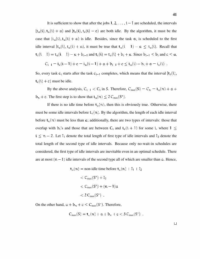
41

It is sufficient to show that after the jobs3, , ''' ,

¦ N 3 are scheduled, the intervals °ç Ì¦P ^ç Ì¦-x and V^Ì¦P VÌ¦-x U are both idle. By the algorithm, it must be the

case that °ç Ì¦P ^ç Ì¦éx is idle. Besides, since the task ¥ is scheduled to the first

idle interval °ç Ì¦P °ç Ì¦Ax , it must be true that ±ç Ì¦ N 3-x ^ç Ì¦ . Recall that

V°Ì¦ N 3K ^ç Ì¦ N 3x x ª¥ 0 / and V^Ì¦Í °ç Ì¦&x ª¥ x . Since ª¥ 0 / ª¥ and U ,

+A¥ 0 / V°Ì¦ N 3Jx U ^ç Ì¦ N 3Jx x ª¥ 0 / x U °ç Ì¦&x ª¥ x V°Ì¦ 'So, every task U°¥ starts after the task U°¥ 0 / completes, which means that the interval

VLÌ¦P V°Ì¦&x U must be idle.

By the above analysis, +-¥ 0 /Ïw+¥ inX

. Therefore, + max X [ + ¬ °ç Åx xª ¬ x U . The first step is to show that ±ç - 7+ max

X T .If there is no idle time before ±ç , then this is obviously true. Otherwise, there

must be some idle intervals before ±ç . By the algorithm, the length of each idle interval

before ^ç must be less than ; additionally, there are two types of intervals: those that

overlap with ª¥ ’s and those that are between +-¥ and V°Ì¦Øx3for some

¦, where

3¦ CN . Let p / denote the total length of first type of idle intervals and p:1 denote the

total length of the second type of idle intervals. Because only no-wait-in schedules are

considered, the first type of idle intervals are inevitable even in an optimal schedule. There

are at most ²N 3 idle intervals of the second type all of which are smaller than . Hence,

°ç K non-idle time before °ç Jx p / x pË1Ï4+ max

X T Jx pË1Ï4+ max

X T Jx N 3 Ïû7+ max

X T 'On the other hand, x ª ¬ x U + max

X T . Therefore,

+ max X Í °ç Jx x ª ¬ x U(ÏÀ¶$+ max

X T 'á

42

Note that if U , then 0N 3 ÇÏ /1 + max

X T . By the above analysis, ±ç Ï³1 + max. Thus, + max

X Ï ô1 + max X T . If U 3

and all task times are integers, then

there is no idle time of the second type before àç , so ^ç ÏÛ+ max X T . Therefore,

+ max X °ç <xg3°x ª ¬ xg3£ ©+ max

X T . The bound of 2 can be achieved asymptotically.

Consider . xE3jobs, where ¥ U^¥ 3

for all34¦g , ª¥ 3

for3Ð¦g

. , and ª1 µ å / Î. . The optimal schedule schedules job . x43first, and all other

jobs completely overlapping with ªÅ1 µ å / . The ratio between the algorithm and the optimal

solution for this instance is3éx µ µ å 1 , which approaches when . is large enough.

Note that Algorithm 1 actually produces order preserving schedules. Since the

minimum order preserving and no-wait-in makespan cannot be smaller than the minimum

no-wait-in makespan, one can obtain the following corollary.


be a schedule produced by Algorithm 1 for a given set of jobs with

preprocessing tasks and postprocessing tasks U and D5ÀU . ThenX

is an order preserving

and no-wait-in schedule and

+ max X

+ max X T ¶

among all order preserving and no-wait-in scheduleX T .

Algorithm 2 - tÏU1. Sort the jobs in nondecreasing order of the processing times of the slave tasks. Sup-

pose the sorted jobs are in the order of3, , ''' , .

2. Schedule task / at time 9 , ªA/ at time and U/ at time x ªA/ .3. Repeat until all jobs are scheduled (see Figure 3.2):

Suppose jobs3, , ''' ,

¦ N 3 have been scheduled. Find the first idle interval / 1

after ^ç Ì¦ N 3x and before +¥ 0 / such that 1±N°/ and 1 x ªJ¥5ú+A¥ 0 / . Schedule

¥ at °/ on the master machine, ª¯¥ at 1 on the slave machine and U±¥ at 1 x ªJ¥ on

43hihhihhihhihhihjijjijjijjijjij kikikkikikkikikkikikkikiklilillilillilillilillilil mimimimimimimimmimimimimimimimmimimimimimimimmimimimimimimimmimimimimimimimnininininininnininininininnininininininnininininininninininininin0 1 2 3 4 5 12 13 16 19 24 2796

a1

a2

a3

a5

c1

c2

c3

c4

c5

a4

Figure 3.2 Illustration of Algorithm 2: jobs are:3"îï¯ ¶ , :3" ¼ ¶ , <3"ü& ¶ , <3"3 9 ¶ and:3"33" ¶ .

(k+2)at (j+1)ct(1)ct

n−1a

(n)atjC nC

nc

C0 opoopoopoopoopoopoqpqqpqqpqqpqqpqqpqrprrprrprrprrprrprspsspsspsspsspsspstptpttptpttptpttptpttptpttptptupupuupupuupupuupupuupupuupupuvvvvvvvwwwwwww

xpxxpxxpxxpxxpxxpxypyypyypyypyypyypyzpzzpzzpzzpzzpzzpzpppppp i

k+1aj−1cjc1c ka2a1a a

naicj+1ck+ma

k+3ak+2

Figure 3.3 Illustration of the proof of Theorem 3.3.3. The idle interval between Uº, 0 / andU^, has length less than ; the idle interval between |' å / and ' å 1 has length less than UANand the idle interval between ' å µ and U°, å / has length less than U .

the master machine. If no such idle interval exists, schedule &¥ at time +A¥ 0 / , ª¥ at

+¥ 0 / x and U^¥ at +A¥ 0 / x x ª¥ .Theorem 3.3.3 Let

Xbe a schedule produced by Algorithm 2 for a given set of jobs

with preprocessing tasks and postprocessing tasks U and ÀÏ U . ThenX

is a feasible

no-wait-in schedule, and

+ max X

+ max X T ¶ú'

Proof : One can use a similar argument as in the proof of Theorem 3.3.1 to show thatX

is a feasible no-wait-in schedule.

Assume that ªÅ, ª¯, å / for3( | N 3 . By the algorithm, +H/[ÏE+1ØÏ4'Ì'd'ºÏ4+ ¬ .

Suppose that +¥ ^ç Ï +A¥ å / for some¦. In order to bound + max

X + max X T , first

consider the length of the idle times between +´, and V^ | x§3 for3t | Ð¦ N 3 . There

are three cases depending on the number of tasks scheduled between +, and V° | xú3 .Assume that ' is the last task scheduled before V° | . See Figure 3.3 for an illustration.

1. There is no task scheduled between +[, and V° | xÀ3 .In this case the whole period between +´, and V° | x3 is idle. It will be proved by

contradiction that VL | x»3 NÀ+-,¯ÏE .

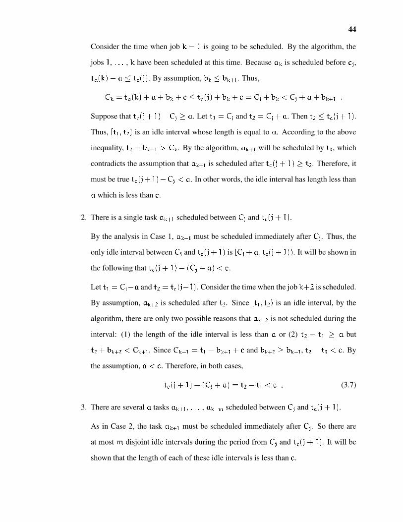
44

Consider the time when job = xú3 is going to be scheduled. By the algorithm, the

jobs3, ''' , = have been scheduled at this time. Because |' is scheduled before U±, ,

°ç = Jx V° | . By assumption, ª' ª-' å / . Thus,

+(' ^ç = Jx x ª-' x U V° | &x ª-' x U +-, x ª-'$Ï4+, x x ª+' å /'Suppose that V^ | x3 NÙ+,Í5ú . Let °/ +, and 1 +, x . Then 1 V^ | xC3 .Thus,

°/ 1 is an idle interval whose length is equal to . According to the above

inequality, 1 x ª+' å /$v +(' . By the algorithm, ' å / will be scheduled by °/ , which

contradicts the assumption that W' å / is scheduled after V° | xl3 5À1 . Therefore, it

must be true V^ | x03 N0+,WÏE . In other words, the idle interval has length less than

which is less than U .2. There is a single task W' å / scheduled between +-, and V^ | x3 .

By the analysis in Case 1, W' å / must be scheduled immediately after +[, . Thus, the

only idle interval between +[, and V° | x3 is +, x V | x«3 . It will be shown in

the following that V^ | x»3 N +-, x Ï»U .Let ^/ +-, x and 1 V^ | x²3 . Consider the time when the job = x is scheduled.

By assumption, ' å 1 is scheduled after 1 . Since °/ 1 is an idle interval, by the

algorithm, there are only two possible reasons that |' å 1 is not scheduled during the

interval: (1) the length of the idle interval is less than or (2) 17Nl°/Ç5 but

1 x ª-' å 1$Ï¾+8' å / . Since +8' å / °/ x ª-' å / x U and ª-' å 1(5»ª-' å / , 1-N°/éÏU . By

the assumption, tÏ»U . Therefore, in both cases,

V^ | x3 N +, x K 1[N¹^/-ÏU' (3.7)

3. There are several tasks W' å / , ''' , ' å µ scheduled between +[, and VL | x»3 .As in Case 2, the task W' å / must be scheduled immediately after +[, . So there are

at most . disjoint idle intervals during the period from +´, and V° | x3 . It will be

shown that the length of each of these idle intervals is less than U .

45

First consider the length of the idle interval between àç = x · ^x and °ç = x · xÇ3 ,where

3) · .N 3 . Without loss of generality, suppose that this interval has length

greater than 9 . If ±ç = x · "x "x UgvC V° | xÙ3 , then the length of the idle interval

is obviously less than U . So one may assume that àç = x · Jx &x U V° | x»3 .

Let 1 í °ç = x · Jx x U and °/ 1´N °ç = x · Jx U . Consider the time

when the job = x · x3 is being scheduled. It is clear that the interval à/ 1 must

be idle at this moment. Since ª*' åJ~^å /é5ûª-' å5~ , it is true that

1 x ª+' å5~Lå / d °ç = x · x Jx U &x ª-' åJ~^å /65^ç = x · Jx x U x ª-' å5~ +(' å5~ 'Thus, by the algorithm, the task W' å5~Lå / must be scheduled at or before ±/ ; that is,

°ç = x · x»3- ^/ °ç = x · Jx U (3.8)

which means that

°ç = x · x3 N ^ç = x · x - UN²ÏUl' (3.9)

For the intervald °ç = x . Åx P ^ç | x3 , one can use the same argument as in

Case 2 to show that the length of the idle time during this period is less than U .Now, one can bound the length of the interval

VL<3P ^ç . The interval consists

of three types of smaller intervals: (i) the intervals occupied by tasks, (ii) the intervals

occupied by U tasks and (iii) idle intervals.

Suppose that W/ , 1 , ''' , * are the tasks scheduled before V°<3 . Then, there are ²N 3 N tasks scheduled during the interval VL<3P ^ç . Therefore, the total length

of the type (i) intervals is ßN 3 N . Recall that it is assumed that +-¥ ^ç Ï4+A¥ å / .

So the number of U tasks during the interval V^<3 °ç is

¦and the total length of the

type (ii) intervals is¦ U .

By Cases 1, 2 and 3, the length of the idle interval after each task is at most U .Since there are

¹N 3 N tasks during the interval V^:3P °ç , the total length of the

idle intervals after these tasks is at most ¹N 3 N U . If there is no task between +é,

46

and +, å / for3) | «¦ N 3 , then there is an idle interval between +[, and +-, å / with length at

most . Since there are¦

jobs that finish before ±ç , the total length of the idle intervals

between the jobs +-, and +, å / with no task between them and3z | §¦ N 3 is at most¦ .

Thus, the length of the interval VL<3P ^ç is

^ç N¹ V^<3K total length of type (i) intervalsx

total length of type (ii) intervals

xtotal length of type (iii) intervals (3.10)

N 3 N x¦ U x7d N 3 N U x¹¦ 'Next, bound VL<3 . By the above assumption, / , 1 , ''' , * are scheduled before

+6/ . Using a similar analysis as in Cases 2 and 3, one can show that ç | x3 NÙ°ç | é U(see (3.8)) for

3( | )N 3 , and V°<3 N °ç Jx Ï»U (see (3.7)). Therefore,

V°:3Í x ªA/ ^ç Jx§ V°<3 N¹^ç - )N 3 U x§ U x Í U x ¾' (3.11)

By (3.11) and (3.10),

°ç Í V^<3Jx °ç NÙ V^<3 V^<3JxÌ N 3 N x¹¦ U x N 3 N U x¹¦ x ªA/ x7d N 3 N x¹¦ U x§ ÇN 3 N U x¦ U x Jx7d N 3 N x¹¦ U x§ N 3 N U x¹¦ N x¹¦ x§ N 3éx¹¦ U à x àyU à x U + max

X T 'Hence,

+ max ^ç Jx x ª ¬ x U 7+ max

X T &x§ x ª ¬ x U - ¶7+ max X T '

á

47

It is not known whether there is a set of jobs achieving a ratio of 3. However, one can

show that the ratio can approach 2 asymptotically. Let . xÀ3, E3 and U 43éx u ,

where u is arbitrarily small. Suppose ª¯¥ 43Ax u for3)«¦6 . and ª1 µ å / . Î x ¶&u .

The makespan of the schedule produced by Algorithm 2 is . Î x ¶&u ^x0 x u . However,

the optimal schedule schedules job . x»3first and all other jobs completely overlapping

with ª1 µ å / . Thus, the optimal makespan is . Î x ¶&u Wx4 x u . If . is very large, the

ratio between the algorithm and the optimal solution can approach arbitrarily closely.

Note that Algorithm 2 produces schedules that are order preserving. Since the min-

imum order preserving and no-wait-in makespan cannot be smaller than the minimum no-

wait-in makespan, Theorem 3.3.3 implies the following corollary.


be a schedule produced by Algorithm 2 for a given set of jobs with

preprocessing tasks and postprocessing tasks U and tÏU . ThenX

is an order preserving

and no-wait-in schedule and

+ max X

+ max X T ¶

among all order preserving and no-wait-in scheduleX T .

CHAPTER 4

APPROXIMATION ALGORITHMS: GENERAL CASES

In this chapter, the total completion time minimization problem will be considered under

various scenarios. This includes single-master systems, multi-master systems, and distinct

preprocessing and postprocessing master systems. Since the problem is strongly NP-hard,

the focus will be on approximation algorithms. For each type of system, both the case

when all jobs have the same release time and the case when the jobs have different release

times will be considered. Algorithms are designed to approximate the best preemptive or

non-preemptive schedules in these cases. The organization of this chapter is as follows. In

Sections 4.3 - 4.5, algorithms are designed to minimize total completion times of preemp-

tive schedules. Section 4.3 is devoted to the single-master case, Section 4.4 is devoted to

the multi-master case, and Section 4.5 is devoted to the case of distinct preprocessor and

postprocessor. In Section 4.6, conversions from preemptive schedules into non-preemptive

schedules will be considered. In section 4.7, linear programming relaxation approach is

applied to systems with distinct preprocessor and postprocessor.

4.1 Preliminaries

An n -approximation algorithm for makespan (or total completion time) is an algorithm

that for any set of jobs generates a scheduleX

whose makespan (or total completion time)

is at most n times the optimal makespan (or total completion time). It is an n ¸ -

approximation algorithm if it is an n -approximation algorithm for makespan and at the

same time a ¸ -approximation algorithm for total completion time. For a scheduleX

, if

+ max X nz+ Tmax and + X - ¸Í+ T , then

Xis said to be an

n ¸ -schedule.

The Shortest-Processing-Time (SPT) rule, which always runs the job with the least

processing time, and the Shortest-Remaining-Processing-Time (SRPT) rule [107, 111],

48

49

which always runs the job with the least remaining processing time, are two well-known

algorithms for minimizing total completion time. Usually, the SPT rule is used to generate

non-preemptive schedules, while the SRPT rule is used to generate preemptive schedules.

Suppose each job consists of a single task. If all jobs are available at time 0, then the SPT

rule is optimal for total completion time in the single-machine or multi-machine environ-

ment. If the release times are arbitrary, then the SRPT rule is optimal for a single machine

and it is a 2-approximation (see [95]) in the multi-machine environment.

In this chapter, both rules will be adapted for the problems in master slave model.

Both are applied to generate preemptive schedules. A scheduling decision is made when an

task or a U task completes so that a master machine becomes free, or when a new task or

a U task becomes available. At any such time instant, the SPT rule schedules, from the set

of available tasks (including those that have been preempted but have not yet completed),

the one with the smallest processing time. Depending on how one chooses from the set of

available jobs, one can obtain theX O ¢ ç rule and the

X O ¢ Vrule. Specifically, in the

X O ¢ çrule, preemption occurs only among the tasks and the preemption is based on the length

of ¥ . In theX O ¢ V

rule, preemption occurs only among the U tasks and the preemption is

based on the length of U°¥ . On the other hand, the SRPT rule schedules, from the set of

available tasks, the one with the smallest remaining processing time. Similarly, one can

define theX+ O ¢ ç rule and the

X+ O ¢ Vrule. Both the SPT rule and the SRPT rule may

generate schedules with migration when there are multiple machines, i.e., after interrupted

on one machine, a task is resumed on a different machine.

In this chapter, the jobs are frequently sorted in certain nondecreasing order of some

parameters Ê¥ of job¦, e.g. Ê¥ U^¥ . For convenience, in this chapter Ê¥KÏûÊ, is used as long

as Êº¥ comes before Ê, in the sorted order, even though it may be the case that Ê¥ Ê, . As in

the previous chapters, one can always assume that the ª tasks are scheduled immediately

when they become available. Thus one can focus on the schedule of tasks and U tasks

only.

50

4.2 New Results and Techniques

Preemptive relaxation and linear programming relaxation are two important techniques for

getting constant-factor approximations for total completion time of non-preemptive sched-

ules; see [95, 59, 14, 45, 109, 108]. Most of these algorithms work by first constructing a

relaxed solution, either a preemptive schedule or a linear programming relaxation. These

relaxations are then used to obtain an ordering of the jobs, and the jobs are list scheduled

(i.e., no unforced idle time) in this order. More about these methods will be discussed in

Section 4.6.

The advantage of the preemptive relaxation is that usually there are very efficient

algorithms to generate optimal or near-optimal schedules. In most cases, these algorithms

(both preemptive and non-preemptive) can be implemented to run in an online fashion, see

[95] and [59]. The linear programming relaxation, however, is more time consuming and

can only be implemented to run in an offline fashion. On the other hand, it provides better

approximation guaranties in some cases. Furthermore, the method usually works even if

one wants to optimize the total weighted completion time; see [59, 14, 45, 109, 108].

Both approaches will be used in this chapter. In all cases, efficient algorithms are

first developed to generate preemptive offline or online schedules with good approximation.

These schedules are shown to have small makespan as well. Then, by applying the ideas in

[95] and [16] to the master slave models, these preemptive schedules can be converted in-

to non-preemptive schedules with certain degradation in the quality of approximation. In

the case when there are distinct preprocessing masters and postprocessing masters, linear

programming relaxation is also used. It is shown that non-preemptive schedules obtained

in this way sometimes have better performance guaranties than those obtained by the pre-

emptive relaxation approach. The results are summarized in Tables 4.1, 4.2, 4.3 and 4.4,

where S is the base of natural logarithm.

51

Table 4.1 New Results for Single-Master System

preemptive non-preemptive

¥ 9 ³1 , canonical ô1 1% 0 / ¥ 9 , non-canonical ¶ Î

¥-5À9 , online and non-canonical ¶ Î

Table 4.2 New Results for Multi-Master System, All Schedules are Non-Canonical

preemptive non-preemptive

¥ 9 ¶ , no migration Î Î

¥-5À9 ¶ , offline with no migrationÌï¯ Î

¥-5À9 ¶ , online with migration -

4.3 Single-master

This section assumes that there is a single master. Canonical schedules are studied first,

and then non-canonical schedules. Finally, the case when jobs have different release times

will be studied. For convenience, throughout this chapter, let ¨ * ¬ , &/ , , È * ¬ ,®/ ª¯,and + *À¬,®/ U°, .

4.3.1 Canonical Preemptive Schedules

First, two lower bounds of the total completion time in canonical schedules are developed.

Suppose there are jobs3, , ''' , . For canonical schedules, whether preemption is

allowed or not, one can derive the following lower bound

+ T 5C6¨ x ¬ê,®/

êV Ó ! V × U^¥ (4.1)

52

Table 4.3 New Results for Distinct Preprocessor and Postprocesor System, .C/ .D1 43

preemptivenon-preemptive

preemptive relaxation LP relaxation

¥ 9 ¶ Î 1% 0 / ¶ îï ¥-5À9 ¶ , offline

Î Î x 1% 0 / Î ¼ ¥-5À9 ¶ , online

Î Î x 1% 0 / -

Table 4.4 New results for distinct preprocessor and postprocesor, .C/65 3 and .2175 3

preemptivenon-preemptive

preemptive relaxation LP relaxation

¥ 9 Î , with migration Î / ³ Î ¼

¥A59 Î ¶ , offline with migrationÌï¯3 ¶ Ìï¯ ½

¥A59 Î ¶ , online with migrationÌï¯3 ¶ -

which assumes that there is no idle time in the schedule and that the U tasks are scheduled

in ascending order of their lengths. Another lower bound is

+ T 5 ¬ê,®&/

êç Ó !&ç × ¥ x È x +

(4.2)

which assumes that jobs are scheduled in increasing order of the J¥ , and that the ª tasks

and the U tasks are scheduled immediately after they are available. Finally, the following

trivial lower bound which is simply the summation of all the processing times holds for any

schedule.

+ T 5û¨ x È x + (4.3)

This follows from the observation that +[,K5ú, x ª¯, x U°, . Summing | from 1 to gives the

result in (4.3).

53

In canonical schedules, all the tasks are scheduled first. Since all the tasks are

available at time 9 and the U tasks cannot start until all the tasks finish, there is no need to

preempt the tasks. Hence, only a U task can be preempted by another U task in this case.

Algorithm Canonical-X O ¢ V

: Schedule the tasks in an arbitrary order without preemp-

tion. After all the tasks finish, schedule the available U tasks by theX O ¢ V

rule.

Theorem 4.3.1 Algorithm Canonical-X O ¢ V

generates a canonical preemptive sched-

ule in ¤ log time.

Proof : Let +Hç × denote the time , completes. Then at time , max ¨ ° +6ç × x ª¯, ,

all the tasks finish and the U±, is available to be scheduled. Since +ç × ¨ , it must be

true that , ¨ x ª¯, . According to the algorithm, if there is another available task U¥ that

hasn’t finished at time , and U^¥KÏU°, , then U°, has to wait until U^¥ finishes. Also, during the

execution of U±, , if there is another task U°¥ÏU°, that becomes available, then U±¥ preempts U°, .In both cases, it is said that U±, is delayed by U°¥ . Let +, be the completion time of U±, in the

schedule generated by Algorithm Canonical-X O ¢ V

. Then,

+, , x U°, x êV Ó delaysV × UL¥

¨ x ª¯, x U°, x êV Ó V × U^¥'The total completion time is

¬ê,®/ +,

¬ê,®&/ Í¨ x ª¯, x U°, x êV Ó V × U^¥ Å¨ x ¬ê

, &/êV Ó V × U^¥ x È x + Ï ©+ T

where the last inequality comes from the lower bounds (4.1) and (4.3).

The above approximation ratio is tight. Consider this example: for3¦Ø N 3 ,

¥ U^¥ u , ª¥ x N 3 u , ¬ U ¬ and ª ¬ u . The optimal canonical

schedule schedules W/ , 1 , ''' , ¬10 / first and then followed by ¬ . The total completion

time is about x3 . However, if one schedules ¬ first followed by W/ , ''' , ¬40 / , then

the total completion time is about à© . (For this example, the optimal preemptive schedule

has the same total completion time as the optimal non-preemptive schedule.)

54

It has been shown in [106] that any canonical schedule without preemption is a -

approximation for makespan. Since preemption among the U tasks can not increase the

makespan, the schedule generated by Algorithm Canonical-X O ¢ V

has makespan at most

two times the optimal. áLet

X / 8 ¦R ¥ U^¥ë; andX 1 8 ¦ ¥év»U^¥B; . Suppose the jobs in

X / are arranged

in increasing order of the ª ’s and the jobs inX 1 are arranged in decreasing order of the ª ’s.

In [106], it was shown that the canonical schedule in which the tasks ofX / are scheduled

before the tasks ofX 1 has makespan at most ¶º° times the optimal schedule. If the

tasks are scheduled in this order in Algorithm Canonical-X O ¢ V

, then one still gets a ¶º° -approximation for makespan, since preemption on the available U tasks will not increase

the makespan.

Corollary 4.3.2 There is an ¤ log time algorithm that generates a ¶º° canonical

preemptive schedule.

Note that when preemption occurs, algorithm Canonical-X O ¢ V

uses SPT rule, in-

stead of the SRPT rule. This is for the purpose of analysis only. In practice, one can use

the SRPT rule to get a better approximation for total completion time.

4.3.2 Non-canonical Preemptive Schedules

In this model, the tasks and the U tasks can be scheduled alternatively. A lower bound on

the + T can be obtained by assuming all the ª tasks have length 9 :+ T 5 ¬ê

,®&/ê

ç Ó å V Ó !&ç × å V × ¥ x U^¥ (4.4)

Algorithm Non-canonical-X O ¢ ç å V : For any two jobs, if

, x U°, Ï ¥ x U^¥ , then

both , and U°, are said to have higher priority than &¥ and U^¥ . At any time, if the master

processor is free for assignment, assign the available task with the highest priority. If a new

task becomes available and has higher priority than the currently running task, the new task

preempts the currently running task.

55

Theorem 4.3.3 Algorithm Non-canonical-X O ¢ ç å V generates a

preemptive schedule

for a single-master system when , 9 for all job | .Proof : Since all the tasks are ready at time 0, there is no need for an task to

preempt another task. Thus, preemption occurs only between a higher priority U task and a

lower priority U task or a lower priority task. Let +Øç × denote the completion time of &,in the schedule generated by Algorithm Non-canonical-

X O ¢ ç å V . If none of the tasks is

preempted by a U task, then +ç × would be , x * ç Ó å V Ó ç × å V ×¥ . Because of preemption,

+6ç × can be delayed by some higher priority U tasks. In other words, Uà¥ can delay , only if

¥ x U^¥Ï , x U°, . At time , +6ç × x ª¯, , the task U°, becomes available. According to the

algorithm, U°, can only be delayed by a task U°¥ such that ¥ x U^¥Ïw, x U°, . Note that if U°¥delays , , it will not delay U±, again. Thus, one can bound the completion time +´, :

+, +6ç × x ª¯, x U°, x êV Ó delaysV × U^¥

êç Ó å V Ó ç × å V × ¥ x êV Ó delays ç × U^¥ x , x ª¯, x U^, x êV Ó delays

V × U^¥ ê

ç Ó å V Ó ç × å V × ¥ x êç Ó å V Ó ç × å V × U^¥ x , x ª¯, x U^,

êç Ó å V Ó ç × å V × ¥ x U^¥ x§ , x ª¯, x U°, '

Therefore, the total completion time is

¬ê,®/ +,

¬ê,®&/ ê

ç Ó å V Ó ç × å V × ¥ x U^¥ x , x ª, x U°, ¬ê

,®/ê

ç Ó å V Ó ç × å V × ¥ x U^¥ x§ ¨ x È x + by (4.4) and (4.3)

©+ T 'To bound the makespan of the schedule, pick the last job | such that U", is scheduled

immediately when it is ready. Such a job always exists since the job¦

with the highest

priority always satisfy this criterion. Then, the interval p/ 9 +6ç × and the interval after

56

U^, starts till the end, i.e., pi1 d +6ç × x ª, P + max, contain no idle time. Denote their lengths

by Ãp / and ÃpË1± , respectively. Then äp/ x ÃpÕ1à + Tmax. Thus, the makespan is

+ max äp / x ª¯, x äpË1± + Tmax

x ª¯,¯Ïû7+ Tmax

á

4.3.3 Arbitrary Release Times

When arbitrary release times are present, it is not meaningful to have canonical schedules

any more. Thus, only non-canonical schedules will be considered. The lower bound (4.4)

still holds for this case. Let *À¬¥Ì/ ¥ . Then, a trivial lower bound for the minimum

total completion time of any schedule is

+ T 5 ¬ê¥Ì/ ¥ x ¥ x ªJ¥ x U^¥ K x ¨ x È x + (4.5)

Observe that Algorithm Non-canonical-X O ¢ ç å V makes no assumptions about the release

time of a job. So, one can still apply Algorithm non-canonical-X O ¢ ç å V when jobs have

arbitrary release times. Unlike the case when all jobs have the same release times, in this

case, a higher priority task may also delay a lower priority task or U task.

Theorem 4.3.4 Algorithm Non-canonical-X O ¢ ç å V generates a

preemptive online sched-

ule for a single-master system even when the jobs have arbitrary release times.

Proof : One can first bound the total completion time of the schedule generated by

Algorithm Non-canonical-X O ¢ ç å V . Let +Hç × be defined as before. Then,

+6ç × , x êç Ó delays ç × ¥

x êV Ó delays ç × U^¥ x ,and

+, +Hç × x ª, x U°, x êç Ó delays

V × ¥x êV Ó delays

V × U^¥ , x ê

ç Ó delays ç × ¥x êV Ó delays ç × U^¥ x , x ª, x U°, x ê

ç Ó delaysV × ¥

x êV Ó delaysV × U^¥

57

êç Ó å V Ó ç × å V × ¥ x U^¥ xú , x , x ª¯, x U°, 2

where the last inequality comes from the fact that the two sets of tasks delaying ¯, and U°,are disjoint, and they all have higher priority than J, and U°, . Similarly, one can bound the

total completion time

¬ê,®/ +,

¬ê,®/ ê

ç Ó å V Ó ç × å V × ¥ x U^¥ xú , x , x ª¯, x U°, ¬ê

,®&/ê

ç Ó å V Ó ç × å V × ¥ x U^¥ x x ¨ x È x + by (4.4) and (4.5)

Ï 7+ T 'To bound the makespan, one picks the last job | such that U, starts immediately after it is

ready. Then the intervals p/ , +6ç × and pË1 Ì +6ç × x ª¯, P + max

must be both busy, and

the total length äp / x äpË1± of these two intervals is at most * ¬ ,®&/ , x * ¬ ,®/ U°, ¨ x + + Tmax. Thus,

+ max , x Ãp~/ x ª, x äpË1± , x ª¯, Jx + Tmax

©+ Tmax 'To conclude the proof, note that Algorithm Non-canonical-

X O ¢ ç å V schedules jobs in an

online fashion. á

4.4 Multi-master

This section assumes that there are .Û5« masters, each of which is capable of processing

both the tasks and the U tasks.

4.4.1 Non-canonical Preemptive Schedules

Let us assume that the jobs are indexed in nondecreasing order of , x U°, . That is, , x U°, , å / x U°, å / for

3£ | N 3 .

58

Algorithm Multi-Master-X O ¢ ç å V : (1) Without loss of generality, one may assume that

is a multiple of . . Otherwise, one can add dummy jobs with &¥ ªJ¥ U^¥ 9 . (2)

Assign the jobs to the machines such that jobs 1, 2, ''' , . go to machines 1, 2, ''' , . ,

respectively; jobs . x3, . x , ''' , . go to machines . , .öN 3 , ''' ,

3, respectively;

jobs . xl3, . x , ''' , ¶º. go to machines 1, 2, ''' , . , respectively; and so on until

all jobs are assigned. (3) Apply Algorithm non-canonical-X O ¢ ç å V to each master machine

to schedule the jobs assigned to it.

Theorem 4.4.1 Algorithm Multi-Master-X O ¢ ç å V generates a

¶ preemptive schedule

for multi-master systems without migration when all jobs have release time 0.

Proof : Without loss of generality, one may assume that .ß= for some integer = .

For convenience, one can reindex the jobs assigned to each machine · in the form of ·

such that ã ~ æ x U ã ~ æ ã ~ å /<æ x U ã ~ å /<æ . A lower bound of the total completion time

comes from the fact that Algorithm Multi-Master-X O ¢ ç å V is optimal if ª ã ~ æ 9 for every

job · .

+ T 5µê ~ / 'ê P/ =¿N x»3 ã ~ æ x U ã ~ æ (4.6)

Fix a machine · . Let + ã ~ æ denote the completion time of job · and È ~ * ' &/ ª ã ~ æ .

Following the analysis of Algorithm non-canonical-X O ¢ ç å V in Section 4.3.2,'ê P/ + ã ~ æ 'ê &/ =¿N x3 ã ~ æ x U ã ~ æ x È ~ '

Thus, the total completion time isµê ~ / 'ê P/ + ã ~ æ µê ~ / 'ê P/ =¿N x3 ã ~ æ x U ã ~ æ Jx È ~ µê ~ / 'ê P/ =¿N x3 ã ~ æ x U ã ~ æ x È by (4.6) and (4.3)

Ï 7+ T '

59

Now analyze the makespan of the schedule. Let ~ * , scheduled on ~ , x U°, . By

the pigeon hole principle, it is easy to see that

min/! ~ ! µ ~ 3. ¬ê,®/ , x U°, ÏE+ Tmax '

For any two machines · and , by the way the jobs are assigned to the machines ~ N max/"!1')! ¬ ' x UJ' N min/"!1')! ¬ ' x UJ' [ max/"!1')! ¬ ' x UJ' ÏE+ Tmax 'This means that for any machine · , ~ min /"!WH! µ x +[Tmax

©+[Tmax. Suppose the

job with the maximum completion time among all jobs is assigned to machine · . Let be

the last job on machine · so that U is scheduled immediately after it is ready. Define +ØçHas before. Then machine · is busy during the intervals p/ 9 +6çH and pË1 d +6çH xª P + max

. The total length of the two intervals is äpP/ x äpË1± ~ Ïû7+[Tmax. Therefore, the

makespan is

+ max äp / x ª x äpË1±ÏÀ¶$+ Tmax '

á

4.4.2 Arbitrary Release Times

Offline schedule without migration In this case, one can still apply Algorithm Multi-

Master-X O ¢ ç å V . However, note that to assign jobs to machines, Algorithm Multi-Master-X O ¢ ç å V requires that one has full knowledge of all the jobs at the beginning. Thus, Al-

gorithm Multi-Master-X O ¢ ç å V is an offline algorithm. One can combine the arguments in

Sections 4.3.3 and 4.4.1 to get the following theorem.

Theorem 4.4.2 Algorithm Multi-Master-X O ¢ ç å V generates a

¶ offline preemptive sched-

ule without migration for multi-master systems when jobs have arbitrary release times.

Proof : Fix a machine · .'ê P/ + ã ~ æ max/!WH!1' ã ~ æ x 'ê P/ =¿N xÀ3 ã ~ æ x U ã ~ æ x È ~ '

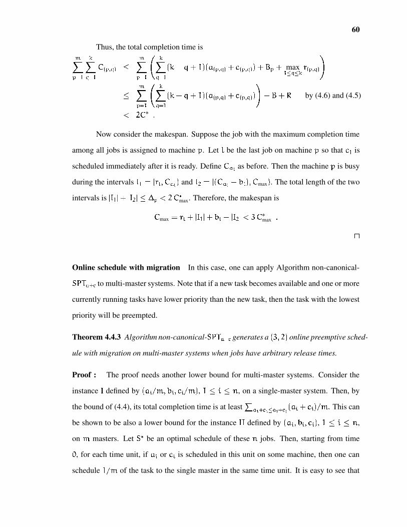
60

Thus, the total completion time isµê ~ &/ 'ê P/ + ã ~ æ µê ~ &/ 'ê &/ =¿N x3 ã ~ æ x U ã ~ æ x È ~ x max/!WH!1' ã ~ æ µê ~ &/ 'ê &/ =¿N x3 ã ~ æ x U ã ~ æ x È x

by (4.6) and (4.5)

Ï + T 'Now consider the makespan. Suppose the job with the maximum completion time

among all jobs is assigned to machine · . Let be the last job on machine · so that U is

scheduled immediately after it is ready. Define +ØçH as before. Then the machine · is busy

during the intervals p/ +6ç and pË1 Ì +Hç x ª P + max. The total length of the two

intervals is Ãp / x äpË1± ~ Ïû7+[Tmax. Therefore, the makespan is

+ max x Ãp~/ x ª x ÃpÕ1°ÏÀ¶$+ Tmax '

á

Online schedule with migration In this case, one can apply Algorithm non-canonical-X O ¢ ç å V to multi-master systems. Note that if a new task becomes available and one or more

currently running tasks have lower priority than the new task, then the task with the lowest

priority will be preempted.

Theorem 4.4.3 Algorithm non-canonical-X O ¢ ç å V generates a

¶ online preemptive sched-

ule with migration on multi-master systems when jobs have arbitrary release times.

Proof : The proof needs another lower bound for multi-master systems. Consider the

instance p defined by ¥Õ. ª¥ U^¥B. , 3z§¦( , on a single-master system. Then, by

the bound of (4.4), its total completion time is at least * ç Ó å V Ó !&ç × å V × ¥ x U^¥ . . This can

be shown to be also a lower bound for the instance pp defined by J¥ ª¥ U^¥ , 3²ú¦¿ ,

on . masters. LetX T be an optimal schedule of these jobs. Then, starting from time

9 , for each time unit, if ¥ or U^¥ is scheduled in this unit on some machine, then one can

schedule3 . of the task to the single master in the same time unit. It is easy to see that

61

the constraint of release time are preserved and that the interval between the finish time of

¥ and the start time of U°¥ is either the same or increased. Thus one obtains a valid schedule

of the instance p on the single-master system. Therefore,

+ T 5 ¬ê,®/

êç Ó å V Ó !&ç × å V × ¥ x U^¥ .

(4.7)

which is a lower bound of the original instance defined by L¥ ¥ ª¥ UL¥ .

Let +6ç × denote the completion time of &, in the schedule generated by Algorithm

non-canonical-X O ¢ ç å V . After , is released at , , it may be delayed by other tasks with

higher priority before it completes. That is, &¥ or U^¥ can delay , only if ¥ x U^¥WÏ4, x U°, . It

is easy to see that there is no idle time on any machine during the interval p/ , ° +6ç × N, ; otherwise, , would have completed earlier. Furthermore, only tasks with higher

priority than | can be scheduled during this interval. At time , +6ç × x ª¯, , the task

U^, becomes ready. Similarly, there is no idle time on any machine during the interval

pÕ1 +6ç × x ª¯, ° +-,¯NlU^, , and only tasks with higher priority than | can be scheduled

during this interval. Note that the task sets in the intervals p/ and pË1 are disjoint. Let Ãp /and äpË1° denote the lengths of p/ and pË1 , respectively. Then, it must be true that äpP/ x äpË1° * ç Ó å V Ó ç × å V × ¥ x U^¥ . . Thus, one can bound the completion time +´, as follows:

+-, , x äp / x , x ª¯, x äpË1± x U^, ê

ç Ó å V Ó ç × å V × ¥ x U^¥ . x , x , x ª¯, x U°, 'The total completion time is

¬ê,®/ +,

¬ê,®/ ê

ç Ó å V Ó ç × å V × ¥ x UL¥ . x§ , x , x ª¯, x U°, ¬ê

,®/ê

ç Ó å V Ó ç × å V × ¥ x U^¥ . x§ x ¨ x È x + by (4.7) and (4.5)

Ï 7+ T 'For the makespan of the schedule, let = be the job with the maximum completion time

among all jobs. Let be the last job among all jobs so that U is scheduled immediately

62

after it is ready. Define +ç as before. Then, all machines must be busy during the intervals

p~/ +6ç N» and pË1 Ì +6ç x ª P + max NUJ' . The total length of the two intervals

is äp / x äpË1° +[Tmax. Therefore, the makespan is

+ max x äp / x x ª x äpË1± x UJ' x x ª Jxú äp / x äpË1° x UJ'$Ïû¶7+ Tmax '

á

4.5 Distinct Preprocessing and Postprocessing Masters

In this section, the model with distinct preprocessing masters and postprocessing masters

will be discussed. Different from the previous cases, here an task can only be preempted

by another task and a U task can only be preempted by another U task. In all cases,

AlgorithmX+ O ¢ ç - X O ¢ V will be applied to obtain a preemptive schedule.

AlgorithmX+ O ¢ ç - X O ¢ V : Schedule the available tasks using the

X+ O ¢ ç rule on the pre-

processing master. Schedule the available U tasks using theX O ¢ V

rule on the postprocessing

master.

Let .0/ and .21 denote the numbers of preprocessing masters and postprocessing

masters, respectively. First the simple case .Ù/ .21 43 will be studied.

Theorem 4.5.1 AlgorithmX- O ¢ ç - X O ¢ V generates a

¶ online preemptive schedule when

.¹/ .D1 E3 and ,K5À9 for all | .Proof : First consider the total completion time. Let +T ç × be the time , finishes in an

optimal schedule. Then,

+ T 5 ¬ê,®/ + T ç × x ª¯, x U°, Í ¬ê

,®/ + T ç × x È x +ð'Let +Hç × be the time , finishes in the schedule obtained by Algorithm

X+ O ¢ ç - X O ¢ V . Since

theX+ O ¢ ç rule is optimal if ªÅ, U°, 9 , Algorithm

X+ O ¢ ç - X O ¢ V must have the minimum

63

*À¬, &/ +6ç × among all possible schedules. That is

¬ê,®/ +6ç ×

¬ê,®&/ + T ç × '

Thus, the total completion time is at most

¬ê,®/ é+Hç × x ª, x U°, x êV Ó delays

V × U^¥ ¬ê,®&/ [ +6ç × x ª¯, x U°, \ x ¬ê

, &/êV Ó V × U^¥ 7+ T '

For the makespan, consider the last job such that U runs immediately when it is available

at time +Hç x ª . There is no idle time in the interval pP/ +6ç and the interval

pÕ1 Ì +Hç x ª P + max. The length of each interval is at most + Tmax. Therefore, the

makespan is

+ max x äp / x ª x äpË1° ¶$+ Tmax '

áTheorem 4.5.2 Algorithm

X+ O ¢ ç - X O ¢ V generates a Î preemptive schedule with mi-

gration when .0/65 3 , .D1©5 3 and , 9 for all | .

Proof : Since all tasks are available at time 9 , then theX- O ¢ ç rule is the same as theX O ¢ ç rule. As mentioned before, the

X O ¢ ç rule is optimal when the ª tasks and the U tasks

have zero length; that is, it minimizes the total completion time of the tasks. Let +6T ç Óbe the finish time of ¥ in an optimal schedule, and let +ç Ó be the finish time of ¥ in the

schedule generated by AlgorithmX+ O ¢ ç - X O ¢ V . Then, as in the case of .Ù/ .D1 3

, a

lower bound of the total completion time is

+ T 5 ¬ê¥Ì/ + T ç Ó x ª¯, x U°, ß ¬ê

¥Ì&/ + T ç Ó x È x + 5 ¬ê¥Ì&/ +Hç Ó x È x + (4.8)

When the task U±, is ready, it can be delayed by a task U±¥ only if U^¥[Ï§U°, . The length of the

intervalÌ +Hç × x ª, P +,N«U°, is at most * V Ó V × V Óµ , since all postprocessing masters must

be busy and can only run the task U±¥ such that U°¥AÏ§U°, during this interval. Hence the total

64

completion time is at most

¬ê,®/ +,

¬ê,®&/ +6ç × x ª¯, x U°, x êV Ó V × U^¥.D1 ß ¬ê

,®/ +6ç ×x È x +O x ¬ê

, &/êV Ó V × U^¥.D1 7+ T

where the last inequality comes from (4.7) and (4.8).

Now the makespan is shown to be at most four times the optimal makespan. As

before, let = be the job with the maximum completion time, and let be the last job such that

the task U runs immediately after it is ready at +çH x ª . Then the intervals p/ 9 +6çHËNÑ and pË1 d +6çH x ª P° + max NUJ' must be both busy. And äpP/ * ç × ç ,ë.0/éÏ + Tmax

and äpË1° * V × V U°,ë.D1ØÏ4+ Tmax. Therefore,

+ max äp / x x ª &x ÃpÕ1° x UI'©Ï«Î£+ Tmax

áTheorem 4.5.3 Algorithm

X+ O ¢ ç - X O ¢ V generates a Î ¶ preemptive schedule with mi-

gration when .0/65 3 , .D1©5 3 and ,K5À9 for all | .Proof : Let + T ç × be the completion time of &, in an optimal schedule. As in the last

section, one can get

+ T 56 ê + T ç × x È x +Let +6ç × be the completion time of , in the schedule generated by Algorithm

X+ O ¢ ç - X O ¢ V .As mentioned before, the

X+ O ¢ ç rule is a -approximation when ªW, U°, 9 . Thus, it

must true that ê +6ç × ê + T ç ×and

¬ê, &/ +,

¬ê,®&/ é+6ç × x ª¯, x U°, x êV Ó V × U^¥Ë.D1

¬ê,®/ +6ç × x È x + x ¬ê

,®&/êV Ó V × U^¥Õ.D1

65

ê + T ç × x ê + T ç × x È x + x ¬ê,®/

êV Ó ! V × U^¥B.21 ¶$+ TNow consider the makespan. As before, let = be the job with the maximum com-

pletion time, and let be the last job such that U runs immediately after it is ready at time

+6çH x ª . Then the intervals p/ +Hç¡±N¹ and pË1 Ì +Hç¡ x ª ° + max N2UJ' must be

both busy. And äp/ * ç × ç ,.¹/[ÏE+ Tmax and äpË1° * V × V U°,.D1ØÏE+ Tmax. Therefore,

+ max x äp / x§ x ª Jx äpË1± x UJ'$ÏÎ©+ Tmax

á

4.6 Converting Preemptive Schedules into Non-preemptive Schedules

As mentioned before, non-preemptive schedules can be obtained by converting preemptive

schedules. Our approach is based on the techniques introduced by Phillips et al. in [95],

and improved by Chekuri et al. in [16]. For completeness, their approaches are described

in the following.

The model studied in [95] consists of one or more identical machines and jobs.

For this model, a general approach of converting a preemptive scheduleX

into a non-

preemptive scheduleX has been given in [95]. The idea is to form a list of jobs in in-

creasing order of their completion times inX

and then list schedule the jobs in this list one

by one, respecting their release times.

Let +, and +, denote the completion time of job | inX

andX , respectively. Sup-

pose the jobs are indexed such that +-¥Ï +¥ å / . Then they showed that +A, +,for a single machine environment and +A, ¶J+, for a multi-machine environment. Let

,max

max /"!¥!", ¥ . The result is based on the observations that (1) +[,¹v ,max, (2)

+,K5 * ,¥Ì&/ ·W¥ in the single-machine case, and +[,K5 * ,¥ë/ ·W¥Ë. in the multi-machine case,

where ·, is the processing time of job | , (3) + , ,maxx * ,¥Ì&/ ·W¥ if there is one machine

and + , ,maxxE * , 0 /¥Ì/ ·Å¥Õ. Åx ·, if there are two or more machines. These results im-

66

ply that ifX

is a ¸ -approximation for total completion time, thenX is a ¸ -approximation

for total completion time in the single-machine environment, and a ¶W¸ -approximation for

total completion time in the multi-machine environment. In addition, this conversion also

yields an online non-preemptive algorithm if the preemptive schedule can be generated on-

line: simply simulate the algorithm for preemptive schedule, start a job | if | completes in

the preemptive schedule or put it in the waiting queue if the machine is busy.

Now, consider the makespan which is equal to the completion time of job inX . It

is easy to see that +¬ + ¬ x * ¬ ,®&/ ·, + ¬ x +[Tmax. Therefore, ifX

is an n -approximation

for makespan, i.e., + max X K + ¬ n´+´Tµ ç Ò , then + max

X A +¬ <3Åx n +[Tmax. In other

words,X is a

<3éx n -approximation for makespan.

Later, Chekuri et al. [16] improved the above results for total completion time. They

designed a deterministic ¤ 1 time offline algorithm such that the schedule obtained has

total completion time at most 0 /¢ 3 ' ï$ times that of the preemptive schedule. They also

gave a randomized online algorithm which generates schedules having expected completion

time 0 / times that of the preemptive schedule. The difference between the two approaches

in [16] and [95] is how to obtain the list of jobs. GivenX

and a parameter £Ù 9 3¤ , let

+(¥, X , the £ -point of | , be the time when £"·Í, (a £ -fraction) of job | is completed. Instead

of forming a list based on +[, X , now form a list based on +O¥, X . A £ -schedule is a non-

preemptive schedule obtained by list scheduling jobs in increasing order of +¦¥, X , possibly

introducing idle time to account for the release times. It is easy to see that the algorithm

given by [95] is a £ -schedule with £ Ð3. It is also clear that a £ -scheduler can be made to

be an on-line algorithm if the underlying preemptive algorithm is an on-line algorithm.

The main result in [16] is that for each given instance, there exists a £ , the best £ ,

such that the £ -schedule has total completion time at most 0 / times that ofX

, and has

makespan at most<3x £ times that of

X. One can obtain such a £ -schedule by finding the

best £ in ¤ 1 time offline deterministically; or one can obtain, through a randomized on-

67

line algorithm, a schedule whose expected total completion time is at most 0 / times that

ofX

and whose makespan is at most<3´x £ times that of

X.

In the multi-machine case, Chakrabarti et al. [14] showed that the convert procedure

given in [95] has a bound of ½à±¶ for total completion time, instead of ¶ times that ofX

.

The following sections describe how to convert preemptive schedules generated in

Sections 4.3-4.5 to non-preemptive schedules. The difficulty of the conversion in the master

slave model is that one needs to respect not only the release time of J¥ , 3(«¦ , but also

respect the constraint that the interval between the finish time of &¥ and the start time of U°¥has length at least ª¯¥ .

4.6.1 Single Master and Multi-Master Systems

First consider the single master systems.

Theorem 4.6.1 In ¤ 1 time, one can obtain a ô1 1% 0 / non-preemptive canonical sched-

ule when there is a single master and L, 9 for all | .Proof : Let

Xbe a preemptive canonical schedule of jobs obtained by applying Corol-

lary 4.3.2. LetX ç be the partial schedule of

Xduring the interval

9 ¨ , andX V

be the

partial schedule ofX V

during the interval ¨ + max

.

ClearlyX ç contains all tasks only. By the Algorithm Canonical-

X O ¢ V, there is no

preemption inX ç . Let +6ç × be the completion time of , . It is easy to see that the partial

scheduleX V

contains all U tasks only and it can be seen as a preemptive schedule of tasks

on a single machine where each task | has a “release time” max ¨ +Øç × x ª¯, and processing

time U°, .To convert

Xinto a non-preemptive schedule

X , one fixesX ç and convert

X Vto a

non-preemptive scheduleX V of U tasks by using the approach of [16]. Let +´, and +, be

the completion time of U±, inX

andX , respectively. As mentioned at the beginning of the

section, it has been shown in [16] that +A, 0 / +, and +, +, x + max. SinceX

is a ³1

68

canonical schedule, the obtained schedule is a ô 1 1% 0 / non-preemptive canonical schedule.

This concludes the proof. áTheorem 4.6.2 In ¤ log time, one can obtain a

¶ Î online non-preemptive sched-

ule when there is a single master and L,K5À9 for all job | .Proof : Let

Xbe a non-canonical preemptive schedule

X. One can get a £ -schedule

X ,£ 3, similarly as [95]: (1) Sort all tasks (both tasks and U tasks) in increasing order

of their completion times. (2) List schedule these tasks on the master machine, with the

constraint that each task &, must start after , and the interval between the time &, finishes

and the time U±, starts is at least ª¯, .For the purpose of analysis, one can visualize the above procedure as follows (see

Figure 4.1): For each task, &, or U°, , remove all but the last scheduled piece of the task.

Suppose the last piece of &, and U°, have length =Wç × and = V × , respectively. Now process the

tasks one by one in the scheduling order of their last pieces inX

. If the current task is ¯, ,complete its last piece by inserting an extra piece with length

,"N0=Åç × immediately after

the last piece of , ; at the same time push backward in time all the last pieces of the tasks

which finish after , inX

by an amount of &,Nû=Åç × . If the task is U°, , complete its last

piece by inserting an extra piece with length Uà,NC= V × immediately after the last piece of

U^, ; at the same time push backward in time all the last pieces of the tasks which finish after

U^, inX

by an amount of U±,JNÀ= V × . Let the schedule be

X . It is easy to see that during

this process, the two constraints, (a) each task J, is scheduled after , and (b) the interval

between the time &, finishes and the time U°, starts is at least ªÅ, , are not violated. ThusX

is still a feasible schedule.

Now one pushes all jobs forward in time as much as possible without changing the

order of the tasks, or violating the constraints (a) and (b) mentioned above. The result

is exactly the scheduleX . Since a task U°, can only be moved back by processing times

associated with tasks finished earlier than Uà, inX

, we have +, +-, and +, +, x

69

131 7 6 10 11 14 15 1916 17 18§O§O§O§O§O§§O§O§O§O§O§§O§O§O§O§O§§O§O§O§O§O§§O§O§O§O§O§ÖÖÖÖÖ¨ÖÖÖÖÖ¨ÖÖÖÖÖ¨ÖÖÖÖÖ¨ÖÖÖÖÖ¨ ©O©O©O©O©O©O©©O©O©O©O©O©O©©O©O©O©O©O©O©©O©O©O©O©O©O©©O©O©O©O©O©O©ªOªOªOªOªOªOªªOªOªOªOªOªOªªOªOªOªOªOªOªªOªOªOªOªOªOªªOªOªOªOªOªOª 12

a3

a1

c3

c1

0 2 3 4 5 6 9

«O«O«O«O«O««O«O«O«O«O««O«O«O«O«O««O«O«O«O«O««O«O«O«O«O«¬O¬O¬O¬O¬O¬¬O¬O¬O¬O¬O¬¬O¬O¬O¬O¬O¬¬O¬O¬O¬O¬O¬¬O¬O¬O¬O¬O¬ OOOOOOOOOOOOOOOOOOOOOOOOO®O®O®O®O®O®®O®O®O®O®O®®O®O®O®O®O®®O®O®O®O®O®®O®O®O®O®O®S

S’

S’’ ¯O¯O¯O¯O¯O¯O¯O¯O¯¯O¯O¯O¯O¯O¯O¯O¯O¯¯O¯O¯O¯O¯O¯O¯O¯O¯¯O¯O¯O¯O¯O¯O¯O¯O¯¯O¯O¯O¯O¯O¯O¯O¯O¯°O°O°O°O°O°O°O°°O°O°O°O°O°O°O°°O°O°O°O°O°O°O°°O°O°O°O°O°O°O°°O°O°O°O°O°O°O°a2

c2

a3

a1

c1

c3

2

±O±O±O±O±O±O±±O±O±O±O±O±O±±O±O±O±O±O±O±±O±O±O±O±O±O±±O±O±O±O±O±O±±O±O±O±O±O±O±²O²O²O²O²O²²O²O²O²O²O²²O²O²O²O²O²²O²O²O²O²O²²O²O²O²O²O²²O²O²O²O²O²a1

a2 a

1a3

0 2 3 4 5 6 9 12 131 7 6 10 11 14

c

5 6 9 12 131 7 6 10 11 14 15 16

a2

c

4

2a3

a1

c1

c3

c1

0 2 3

Figure 4.1 Convert a preemptive schedule into a non-preemptive schedule:X

is a pre-emptive schedule of three jobs

# / 9 Î , # 1 3" 3 , # ³ Î Î ; X is the non-preemptive schedule obtained from

Xby completing the last piece of each task into a whole

piece;X is the non-preemptive schedule obtained from

X by removing unnecessary idleintervals in

X .* ¬ ¥Ì/ ¥ x U^¥ - +-, x + max, where +N, is the completion time of U±, in

X . This implies that

if one takes the non-canonical schedule in Theorem 4.3.4, then one can get a

¶ Î non-preemptive schedule. Furthermore, it can be implemented online if the preemptive

schedule is online. áThe following theorem shows how to get offline non-preemptive schedules for

multi-master systems. It is not known how to obtain an online non-preemptive schedule.

Theorem 4.6.3 When there are multi-masters, one can obtain aÌï¯ Î non-preemptive of-

fline schedule.

Proof : LetX

be the (2,2)-schedule generated by Algorithm Multi-Master-X O ¢ ç å V . ThenX

has no migration. One can obtain the non-preemptive scheduleX by converting the

schedule on each machine separately in the same way as described in the proof of Theo-

rem 4.6.2. Thus, the total completion time ofX is at most two times that of

X. Since

Xis

a -approximation for total completion time,X is a Î -approximation for total completion

time. For the makespan, +A, +, x maxµ¥Ì/ 6¥ where 6¥ is the total length of the tasks

and the U tasks assigned on machine¦. In Section 4.4, it has been shown that ¥ ©+ Tmax.

Thus, + , +, x maxµ¥Ì&/ 6¥ +, x 7+ Tmax. Since

Xis ¶ -approximation for makespan,

X is a

ï-approximation for the makespan. This concludes the proof. á

70

4.6.2 Distinct Preprocessors and Postprocessors

This subsection considers the case when there are ./ preprocessors and .21 postprocessors.

Theorem 4.6.4 In ¤ 1 time, one can obtain a Î 1% 0 / non-preemptive schedule when

, 9 for all | , and .0/ .D1 E3 .Proof : Let

Xbe the

¶ -schedule generated by AlgorithmX+ O ¢ ç - X O ¢ V . Since , 9

for all | , there is no preemption on the single preprocessor. Let +ç × be the completion time

of , inX

. To get a non-preemptive schedule, one can fix the schedule of the tasks and do

the conversion simply on the single postprocessor using exactly the approach given in [16],

respecting the “release time” of task Uà, +6ç × x ª¯, . Following exactly the same argument,

one can show thatX is a

Î 1% 0 / non-preemptive schedule. áWhen the release times are arbitrary, one needs to do the conversion carefully so as

to make sure that the difference between the finish time of J, and the start time of U±, is at

least ª¯, .Theorem 4.6.5 When .Ù/ .D1 3

, and ,5 9 , one can obtain a Î Î x 1% 0 / non-

preemptive offline schedule or an online non-preemptive schedule with expected perfor-

mance Î Î x 1% 0 / .

Proof : LetX

be the ¶ -schedule generated by Algorithm

X- O ¢ ç - X O ¢ V . Let +, be the

completion time of job | inX

. Let +ç × be the completion time of &, inX

.

The conversion consists of two steps. First one can remove the preemptions among

the tasks to get the best (offline) £ -schedule of the tasks on the single preprocessor by

using the approach of [16]. Let +Nç × be the new completion time of , . Then, one must have

+ç × 0 / +6ç × . Now fix the schedule of tasks, and remove the preemptions among the Utasks to get a £ -schedule of the U tasks, where £ w3

, and make sure the interval between

+ç × and the start time of U±, is at least ªÅ, for each job | .Suppose the jobs are indexed so that +[¥Ï4+A¥ å / . Then, +-,5 max

max

,¥Ì&/ ¥ max,¥Ì&/ ª¥

* ,¥Ì/ ¥ * ,¥Ì/ U^¥ . Let the new schedule beX and let the completion time of Uà, in

X be

71

+, . Then

+ , + ç × x max/"!¥!", ªJ¥ x ,ê¥Ì&/ U^¥

0 / +6ç × x 7+-, x 0 / +-,z'Thus, * ¬ , &/ +, ¾ x 0 / * ¬ ,®&/ +, . By assumption,

Xis -approximation for total com-

pletion time. Thus,X is

Î x 1% 0 / -approximation for total completion time.

For the makespan,

+ , max/"!¥!", ¥ x êE = ÓF! E = × ¥ x max/"!¥!", ª¥ x ,ê¥Ì&/ U^¥

Î£+ Tmax 'Thus,

X is a Î Î x 1¤ 0 / non-preemptive offline schedule. Similarly as in [16], one can

also get an online schedule whose expected performance is Î Î x 1¤ 0 / . This concludes

the proof. áTheorem 4.6.6 In ¤ log time, one can obtain a

Î 3 Î±¶ non-preemptive schedule

when , 9 for all | , .0/65 3 and .2175 3 .Proof : Let

Xbe the

Î -schedule generated by AlgorithmX+ O ¢ ç - X O ¢ V . Since all

jobs have the same release time, no preemption occurs on the preprocessors. Now fix the

schedule of the tasks. Let +ç × be the completion time of , inX

. The task U°, can be seen

as a task with release time +ç × x ª¯, . The conversion is performed on the postprocessors

using the approach given in [95], subject to the constraint that U", can not start earlier than

its “release time” +Hç × x ª¯, . Then by [14], the total completion time of

X is at most K³times that of

X, i.e.,

X is a / ³ -approximation for total completion time.

Now consider the makespan. Suppose the jobs are indexed such that +´¥ +A¥ å /inX

. By the algorithm, for any3¹ ¦b , +ç Ó x ª¥ * 'J³¥ 'L.¹/ xí ¥ x ªJ¥ z

7+ Tµ ç Ò and * ,¥ë/ U^¥Ë.D1 + Tµ ç Ò . InX , the latest time the postprocessors become busy is

max ¥!", +Hç Ó x ª¥ . Therefore, +N, max ¥!", +6ç Ó x ªJ¥ x * , 0 /¥Ì&/ U^¥Ë.D1 x U°, Î¯+[Tmax. áTheorem 4.6.7 In ¤ log time, one can obtain a

Ìï¯3 ¶ non-preemptive online sched-

ule when .0/65 3 and .2175 3 .

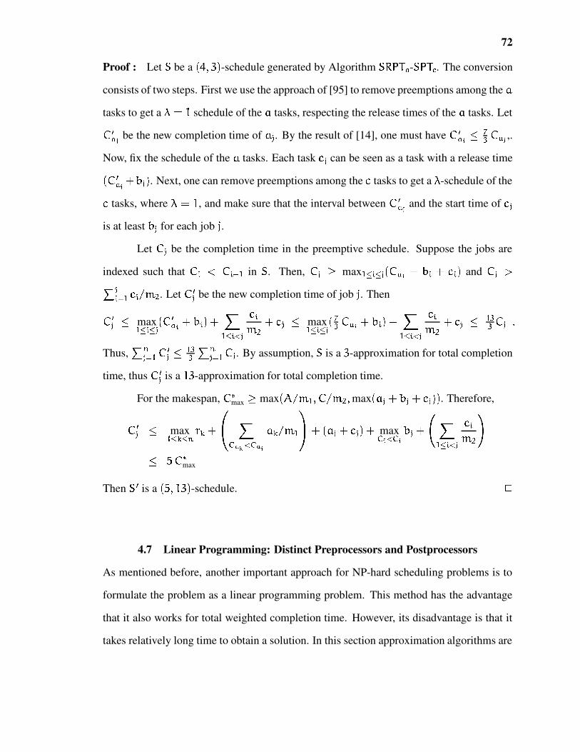
72

Proof : LetX

be a Î ¶ -schedule generated by Algorithm

X+ O ¢ ç - X O ¢ V . The conversion

consists of two steps. First we use the approach of [95] to remove preemptions among the tasks to get a £ 43 schedule of the tasks, respecting the release times of the tasks. Let

+ç × be the new completion time of , . By the result of [14], one must have +Aç × K³ +6ç × ,.Now, fix the schedule of the tasks. Each task U, can be seen as a task with a release time + ç × x ª¯, . Next, one can remove preemptions among the U tasks to get a £ -schedule of the

U tasks, where £ 3, and make sure that the interval between + ç × and the start time of U±,

is at least ªÅ, for each job | .Let +, be the completion time in the preemptive schedule. Suppose the jobs are

indexed such that +¥bÏ +A¥ å / inX

. Then, +,25 max /"!¥!", +6ç Ó x ª¥ x U^¥ and +,2v* ,¥Ì/ UL¥Õ.D1 . Let +, be the new completion time of job | . Then

+ , max/"!¥!", + ç Ó x ª¥ Jx ê/"!¥ , U^¥.D1 x U°, max/"!¥!", K³ +6ç Ó x ª¥ Jx ê

/"!¥ , U^¥.21 x U^, / ³³ +,t'Thus, *À¬, &/ +, / ³³ *À¬,®&/ +, . By assumption,

Xis a ¶ -approximation for total completion

time, thus +, is a3 ¶ -approximation for total completion time.

For the makespan, +´Tmax 5 max ¨.¹/ +[.D1 max

, x ª¯, x U°, . Therefore,

+ , max/"!1')! ¬ ,' x êE = B E = × '.¹/´ x , x U^, Jx maxE Ó E × ª¯, x ê

/"!¥ , U^¥.D1 ï + Tmax

ThenX is a

Ìï¯3 ¶ -schedule. á

4.7 Linear Programming: Distinct Preprocessors and Postprocessors

As mentioned before, another important approach for NP-hard scheduling problems is to

formulate the problem as a linear programming problem. This method has the advantage

that it also works for total weighted completion time. However, its disadvantage is that it

takes relatively long time to obtain a solution. In this section approximation algorithms are

73

presented for the case when there are distinct preprocessing and postprocessing processors.

Each job | is allowed to have a weight , .The basis of the approximation algorithms in this section is a linear programming

relaxation that uses as variables the completion times of the tasks and the U tasks. For

each task | , define +Hç × and +, to be the completion time of &, and U°, , respectively. The

total weighted completion time minimization problem can be formulated as follows:

minimize¬ê,®/ ²,:+, (4.9)

subject to

+6ç × 5« , x , (4.10)

+,Í5ú+6ç × x ª¯, x U°, (4.11)

+-,D5 +(' x U°, or +8'ú5 +-, x UJ' for each pair | j = (4.12)

+Hç × 5 +Hç B x , or +Hç B 5 +6ç × x ' for each pair | j = (4.13)

4.7.1 .0/ .D1 E3The difficulty with the above characterization is the so-called “disjunctive” constraints

(4.12)-(4.13), which are not linear inequalities and cannot be modeled using linear inequal-

ities. Instead, one can use a class of valid inequalities for any feasible schedules (maybe

preemptive), introduced by Queyranne [98] and Wolsey [119]. Suppose a setk

of tasks,

denoted by3, , ''' , , are scheduled on a single machine. Let ·, be the processing time

of | and +-, be the completion time of | in any feasible schedule. Then, the following in-

equality is valid for any subset É¶µ k .

ê, ÔÖ ·W,:+,K5

3 ê , ÔÖ · 1 , x ê

, ÔÖ ·, 1 for each Éµ k (4.14)

74

The key to the quality of the approximation deriving from the above relaxations is

the following lemma.

Lemma 4.7.1 ([59],[108]) Let +/ , +A1 , ''' , + ¬ satisfy (4.14), and assume without loss of

generality that +/-Ï +A1ØÏ4'''àÏ + ¬ . Then, for each job | E3 , ''' , ,

+-,K5 3,ê '/ ·.'

A feasible solution +/ÑÏ +A1Ï'''[Ï + ¬ satisfying (4.14) need not correspond

to a feasible schedule. Lemma 4.7.1 states that merely satisfying the constraints (4.14) is

sufficient to obtain a relaxation of this: +´,5 /1 * ,'/ ·.' .Queyranne [98] has shown that the linear program with constraints (4.14) is solv-

able in polynomial time via the ellipsoid algorithm; the key observation is that there is a

polynomial time separation algorithm for the exponentially large class of constraints given

by (4.14).

In our model, one can apply the above constraints to the preprocessing master and

the postprocessing master, respectively.

ê ' ÔÖ '+Hç B 5 3 ê , ÔÖ 1 , x3 ê

, ÔÖ , 1 for each É¶µ k (4.15)

ê ' ÔÖ UJ'à+('5 3 ê , ÔÖ U 1 , x6 ê

, ÔÖ U°, 1 for each Éµ k (4.16)

Algorithm List-Schedule-Guided-by-LP-Single-Master: First obtain an optimal solu-

tion to the linear program formed by (4.9), (4.10), (4.11), (4.15) and (4.16). Denote the

completion time of the jobs by +Ø/ , ''' , + ¬ . Then one can form a schedule by scheduling

both the tasks and the U tasks in increasing order of +´, under the condition that , can

not start until , , and the interval between the start time of Uà, and the finish time of , is at

least ª¯, , i.e., U°, can not start until ªÅ, finishes.

75

Theorem 4.7.2 Suppose that .Ù/ .D1 3. Then Algorithm List-Schedule-Guided-by-

LP-Single-Master produces a ¶ îï -schedule when all jobs have the same release time and Î ¼ -schedule when each job has an arbitrary release time. Furthermore, the tasks and

the U tasks complete in the same order.

Proof : LetX

be the schedule obtained by Algorithm List-Schedule-Guided-by-LP-

Single-Master. Let +Hç × be the completion time of &, inX

. By the way the tasks are

scheduled, we have +Hç × max ')!",Â8Ë )'; x * ')!", ' since the latest time the preprocessor be-

comes busy is max ')!",®8i ,'; . Let +, be the completion time of job | inX

. Because the U tasks

are scheduled in the same order as the tasks, it is possible that U, can not start even af-

ter ª¯, finishes at +6ç × x ª¯, . This is because U±, 0 / may not have completed yet. However, the

time that U±, needs to wait after it is ready is at most max ')!",®8:ª-'; x * ')!", 0 / UJ' . Thus,

+, +Hç × x max')!", 8rª-'; x , 0 /ê '/ UJ' x U°,

max')!", 8Ë )'; x ,ê '&/ ' x max')!", 8rª-'; x ,ê '/ UJ'max')!", 8Ë )'; x +6ç × x max')!", 8:ª-'; x +, by Lemma Î¯' ½' 3

max')!", 8Ë )'; x¹ï +,

Thus, if all jobs have the same release times, then +´, 4ï +, ; otherwise, +, ¼ +, . This

implies thatX

is aï-approximation for total completion time when ^, 9 for all | , and a

¼ -approximation when ,59 . This is so even if each job | has a weight.

For the makespan,

+, +6ç × x max')!", ª-' x ,ê '&/ UJ'

max')!", 8i ,'; x ,ê '/ ', x max')!", 8rª-'; x ,ê '&/ UJ'max')!", 8Ë )'; x ¶J+ Tmax

Thus, if all jobs have the same release times, then +´, ¶J+ Tµ ç Ò ; otherwise, +-, Î¯+ Tmax. á

76

4.7.2 .0/5 3 and .D1©5 3If the jobs are scheduled on . machines, then similar valid inequalities hold which were

also observed by Queyranne [99].

ê ' ÔÖ ·.'"+(')5 3. ê , ÔÖ · 1 , x ê

, ÔÖ ·, 1 for each É¶µ k (4.17)

One can derive similar lemma as in the single machine case.

Lemma 4.7.3 Let +H/ , +A1 , ''' , + ¬ satisfy (4.17), and assume without loss of generality

that +H/-Ï +A1ØÏE'''Ï + ¬ . Then, for each job | 43 , ''' , ,

+-,5 3.

,ê '/ ·.'In our model, one can apply the above constraints to the .C/ preprocessing masters

and the .21 postprocessing masters, respectively.

ê ' ÔÖ '"+6ç B 5 3.¹/ ê , ÔÖ 1 , x ê

, ÔÖ , 1 for each É¶µ k (4.18)

ê ' ÔÖ UI'"+('5 3.D1 ê , ÔÖ U 1 , x6 ê

, ÔÖ U°, 1 for each É¶µ k (4.19)

Algorithm List-Schedule-Guided-by-LP-Multi-Master: First obtain an optimal solu-

tion to the linear program given by (4.9), (4.10), (4.11), (4.18) and (4.19). Denote the

completion time of the jobs by +/ , ''' , + ¬ . Schedule both the tasks and the U tasks one

by one in nondecreasing order of +é, under the condition that: , can not start until , , and

the interval between the finish time of &, and the start time of U°, is at least ªÅ, . In other

words, U°, can not start until ªÅ, finishes.

Theorem 4.7.4 Suppose that .Ù/5 3 and .D1©5 3 . Then Algorithm List-Schedule-Guided-

by-LP-Multi-Master produces a Î ¼ -schedule when all jobs have the same release time

andÌï¯ ½ -schedule when each job has an arbitrary release time.

Proof : LetX

be the schedule obtained by Algorithm List-Schedule-Guided-by-LP-Multi-

Master. Let +Hç × be the completion time of task &, inX

. By the way the tasks are

77

scheduled, the latest time the preprocessor becomes busy is max ')!",Â8Ë )'; . Then ' , = |PN 3 ,are scheduled one by one. By time max ')!",Â8Ë )'; x * ')!", 0 / 'L.¹/ , the first |ÅN 3 tasks

must be finished and there will be an idle machine to process the |"·¸ task. Thus, +Hç × max ')!", 8i ,'; x * ')!", 0 / 'L.¹/ x , . Let +-, be the completion time of job | in

X. Because

the U tasks are scheduled in the same order as the tasks, it is possible that U", can not start

even after ª¯, finishes at +6ç × x ª, , because U°, 0 / may not have completed yet. However, the

time that U±, needs to wait after it is ready is at most max ')!",®8:ª-'; x * ')!", 0 / UJ'L.D1 . Thus,

+, +6ç × x max')!", 8rª-'; x 3.D1

, 0 /ê '&/ UJ' x U°,

max')!", 8i ,'; x 3.0/

, 0 /ê '/ ' x , x max')!", 8rª-'; x 3.D1

, 0 /ê '/ UI' x U°,max')!", 8Ë )'; x max')!", 0 / +6ç B x max')!", 8rª-'; x +, xú , x U°, max')!", 8Ë )'; x ¼ +,

Thus, if all jobs have the same release times, then +´, ¼ +, ; otherwise, +-, ½ +, . Thus,X

is a ¼ -approximation for total completion time when ^, 9 for all | , and a ½ -approximation

when ,5»9 . This is so even if each job | has a weight , .Now consider the makespan.

+, +6ç × x max')!", 8rª-'; x 3.D1

, 0 /ê '&/ UJ' x U°,

max')!", 8i ,'; x 3.0/

, 0 /ê '/ ' x , x max')!", 8rª-'; x 3.D1

, 0 /ê '/ UI' x U°,

max')!", 8Ë )'; x 3.¹/

, 0 /ê '/ ' x max')!", 8rª-'; x 3.D1

, 0 /ê '/ UJ' x§ , x U°, max')!", 8Ë )'; x Î¯+ Tmax

Thus, if all jobs have the same release times, then +´, Î¯+ Tµ ç Ò ; otherwise, +-, «ï + Tmax. á

PART II

NETWORK DESIGN PROBLEMS

78

CHAPTER 5

POLYNOMIAL-TIME APPROXIMATION SCHEMES FOR THE EUCLIDEAN

SURVIVABLE NETWORK DESIGN PROBLEM

5.1 Introduction

This chapter considers the geometric version of the survivable network design problem.

The input vertices are assumed to be points in M and the cost of each link is equal to

the Euclidean distance between its endpoints (which is a good approximation in many

applications, since often the “installation” and the “service” cost is roughly proportional to

the length of the link [91]).

The focus is on two most basic variants of the geometric survivable network design

problem: (1) SMT problem in which (b8:9 3 ; for any b and (2) 8:9 3" "; -vertex- and

-edge-connectivity problem in which Ñ8:9 3" "; for all . Note that SMT problem

is a special case of 8:9 3" "; -vertex- and -edge-connectivity problem.

The arguments provided by Grotschel et al. [53] (see also [91, 113]), suggest that

the second special case in the above models well many applications of the survivability

problem, e.g., the problem of designing survivable fiber telephone networks [91, 113]. In

the case of fiber communication networks for telephone companies, network topologies

with connectivity requirements in 8<9 3" "; provide an adequate level of survivability for

the distinguished central nodes of connectivity type 2. Simply, most failures usually can

be repaired relatively quickly and, as statistical studies have revealed, it is unlikely that a

second failure will occur for their duration.

5.1.1 Related Works

There has been a lot of research on the survivable network design problem. Typically,

the research addresses either practical heuristics and algorithms (see, e.g., [21, 50, 51, 53,

53, 91, 113]) or the general problem for arbitrary networks (see, e.g., [36, 37, 41, 64,

79

80

117]), or the problem restricted to very specific networks. In particular, the result due

to Jain [64] gives a polynomial-time -approximation algorithm for the edge-connected

survivable network design problem (for arbitrary connectivity requirements). Also, poly-

nomial-time -approximation algorithms for arbitrary networks in the case Çß8<9 3" ";for every have been recently presented [36, 37]. There is no other good polynomial-

time approximation algorithm specialized for the geometric version of the survivability

problem except the case when û8:9 3 ; for every [97]. If û8:9 3 ; for every and ¹ 8ë 6 Ä3 ; , then one can easily show that a minimum spanning tree of¹ guarantees the approximation ratio of in any metric space (and thus, in particular, in

any Euclidean space M ). Importantly, in this case the geometric survivability problem

is a generalization of the classical Euclidean (complete) Steiner tree problem (see, e.g.,

[44, 62, 63, 97, 118]). The Euclidean (complete) Steiner tree problem for a finite set of

pointsX

in M is to construct a minimum length tree whose vertex set consists of all points

inX

and possibly some other points in M . Thus, the latter problem can be regarded as a

survivable network design problem on an infinite vertex domain, i.e.,E M7 and í3

for any y X , and 9 otherwise. By the celebrated results due to Arora [3] and Mitchell

[90] (see also [101]), the Euclidean (complete) Steiner tree problem admits a polynomial-

time approximation scheme for any constant

.

5.1.2 New Contributions

The first polynomial-time approximation schemes (PTASs) are designed for the two afore-

mentioned basic variants of the geometric survivable network design problem.

First, the simplest case in which £y8<9 3 ; for any vertex y is considered, that

is, the Steiner tree problem. An algorithm is designed such that that for any constant

and

any constant u , it returns a Steiner tree whose cost is at most<36x u times larger than the

minimum. The algorithm runs in timeb log . For general

and u , its running time isb log u »º ã æ Jxb u ã ¤¼ s<æ¾½ ¿ÁÀ ¡Â .

81

Next, the case when 2«8:9 3" "; for any vertex « is considered; this is the

classical problem investigated thoroughly by Grotschel and Monma et al. [50, 51, 52, 53,

91, 113]. The algorithm for the Steiner tree problem is extended to design an algorithm

that, for any constant

and any constant u , returns a graph satisfying all the vertex (or

edge, respectively) connectivity requirements and having the cost at most<37x u times

the minimum. The algorithm runs in timeb log . When

and u are allowed to vary

arbitrarily, its running time isb log u "º ã æ Jx«D u ã %¼ s<æ ½ ¿À Â .

Finally, observe that the techniques yield also a PTAS for the multigraph variant

where the edge-connectivity requirements satisfy )y8:9 3" ''' =; and = §b<3 .All the polynomial-time approximation schemes in this chpater follow an approach

similar to those used in the recent PTASs for finding TSP, (complete) Steiner trees, and

minimum-cost biconnected spanning subgraph in Euclidean graphs, see [3, 26, 101]. How-

ever, there are many important differences that make the new results significantly more

complicated. First of all, one has to deal with the restriction of the Steiner points to the set

given a priori (unlike in the minimum-cost Euclidean (complete) Steiner trees problem, in

which Steiner points are allowed to be any points in M ). Furthermore, one has to deal with

non-uniform connectivity requirements. The substantial differences and complications oc-

cur in the so called filtering phase and searching phase (dynamic programming).

All the PTASs are randomized and achieve the promised approximation guarantees

and running time on the average. However, all these algorithms can be derandomized in

a way similar to that used by Rao and Smith in [101]. The derandomization preserves the

running time ofb log for constant

and u .

5.2 Definitions

Following are some notations and definitions for Euclidean (geometric) graphs that will be

used in this chapter.

82

A Euclidean graph, which frequently will be called in this chapter a graph, is a

pairwÕOJP

, whereO

is a set of points in a Euclidean space M and

is a subset of

the pairs of points inO

. Every Euclidean graph is weighted and the cost of edge Ê T is

equal to the Euclidean distance between points Ê and T . The cost of the graph is the sum of

the costs of its edges. Additionally, Euclidean multigraphs, which are as Euclidean graphs

but may contain parallel edges, are also considered. Consistently with the definition, the

edges of a Euclidean graph or multigraph BOP

are in one-to-one correspondence

with the straight-line segments (in M ) connecting the incident vertices. (Such graphs are

frequently called straight-line graphs in the literature.) Sometimes, for technical reasons,

it is also allowed to bend some edges. A bent edge between a pair of points inO

will be

identified with a straight-line path (a path consisting of straight-line segments connecting

the points).

Spanners for general graphs have been defined in Chapter 1. In this chapter, geo-

metric spanners of a set of points are considered.

Definition 5.2.1 (Geometric spanners) LetO

be a set of points in M . A graph

onO

is

called a geometric -spanner ofO

, z5 3, if for any pair of points · O there exists a

path in

from · to of length at most times the Euclidean distance between · and .

Since only geometric spanners are considered. For simplicity, a geometric spanner

is simply referred to as a spanner. The following result is proven in [56]1.

Lemma 5.2.2 [56] LetO

be a set of points in M , where

is a constant. Let u be any

positive constant. Then, there exists anb log -time algorithm that finds a

:3$x u -spanner of

Ohaving constant maximum degree and the total cost of order of the minimum

spanning tree ofO

.

1Notice that the algorithms used in Lemma 5.2.2 are in the so-called real RAM model, which is thealgebraic decision tree model extended with indirected addressing [56]. If one assumes the algebraicdecision tree model, then the running time will be by a factor of log ÃÅÄ log log Ã larger [56].

83

For arbitrary

and u , the running time of this algorithm isDÆ s è x è è log

and the resulting:3Wx u -spanner of

Ohas maximum degree upper bounded by Ç s and the

total cost upper bounded by Ç s times the cost of the minimum spanning tree ofO

, whereÆ s ¾ u º ã æ and Ç s u º ã æ .Definition 5.2.3 Leapfrog property ([30]) Let ß5öØv 3

.

is a set of line segments

in

-dimensional space.

satisfies the leapfrog property if the following is true for

every possible subsetX 8 P^ P^P° / / P ''' ° µ µ ; of

:

è P P Ï ê/"!¥! µ -¥Âº¥ x è µ P x êP !¥! µ 0 / ¥ë-¥ å / '

Informally, this definition says that if there exists an edge between P and P , then

any path not including P° P^ must have length greater than è P P .

Lemma 5.2.4 ([30]) If a set of line segments

in

-dimensional space satisfies the -

leapfrog property where ©5 v 3 , then the weight of

isD ² :¡ X¢ where ² :¡ X¢

is the cost of a minimum spanning tree connecting the endpoints of

. The constant implicit

in the

- notation depends on and

.

Definition 5.2.5 (Steiner trees) LetO / be a set of points in M . A Euclidean tree is called

a Steiner tree ofO / if its vertex set includes all the points

O / . All the vertices of a Steiner

tree ofO / outside

O / are called its Steiner points. If the Steiner points are restricted to a

point setO-P

, the tree is called a Steiner tree ofO / with respect to

O-Pand the points in

O-Pare called Steiner point candidates.

Definition 5.2.6 (Euclidean (complete) Steiner trees) LetO

be a set of points in M$ . The

Euclidean (complete) Steiner minimal tree ofO

is a Steiner tree ofO

having the minimum

cost.

84

Definition 5.2.7 (Steiner minimum trees (SMT)) LetOíOP8ÈO / be a point set in the

Euclidean space M . A Steiner tree ofO / with respect to

O-Phaving the minimum cost will

be called a Steiner minimum tree (SMT) ofO / with respect to

O-P.

Observe the difference between the definition of Euclidean (complete) Steiner tree

and Steiner minimum tree; in this chapter the abbreviation SMT is used only to denote a

Steiner minimum tree.

As mentioned before, the focus in this chapter is on the variant of the problem

when ~ û8:9 3" "; for any ·4 O . This problem is called the 8<9 3" "; -vertex- or -edge-

connectivity problem, depending on whether the vertex-connected or the edge-connected

version of the problem is considered. (Notice that the 8:9 3" "; -vertex- and -edge-connectivity

problem includes the SMT problem in which ~ 48:9 3 ; for any · O(see Definition

5.2.7).) Furthermore, one can repeat the arguments used in [26] (which were also used

earlier in [38, Section 3]) to show that in metric spaces 8<9 3" "; -vertex-connectivity and

8:9 3" "; -edge-connectivity are essentially equivalent (the arguments in [26] and [38] were

given only for biconnectivity vs. two-edge-connectivity).

Lemma 5.2.8 LetO-PPO / PO 1 be any three sets of points in a metric space. Let R be a

multigraph with the vertex setOP8ÈÇO / ÈO 1 such that for any pair of vertices § O ¥ and

ú O , there are at least min8 ¦ |Ë; 9 ¦ | edge-disjoint paths from to in R .

Then, in linear time, one can transform R into a graph

without increasing the total cost

such that for any pair of vertices § O ¥ and ¹ O , there are at least min8 ¦ |i; internally

vertex-disjoint paths form to in

.

Proof : Initially setû R and a sequence of modification will be performed to transform

to get the required properties. It is easy to see that if û OPÅÈ2O / , then graph

already

has the required properties with respect to . Therefore one only has to deal with points

O 1 all of which are in the same two-edge-connected component of

. If this single

component is also a block, it is done; otherwise pick any two edges and

such

85

that and are in different blocks, in other words, is an articulation point. Replace

edges and

by . Now, and will be in the same block. By the triangle

inequality, the cost of the new block will not be larger than the sum of the older two blocks.

One does this replacement until all points ofO 1 are in the same block. Then remove all

parallel edges from the graph, and

becomes a graph has a cost not greater than that of

R , and for any pair of vertices O ¥ and O , there are at least min8 ¦ |Ë; internally

vertex-disjoint paths form to in

.

Using standard techniques this transformation can be performed in time linear in

the number of edges in R . áThis lemma allows one to concentrate only on the 8<9 3" "; -edge-connectivity prob-

lem, and to allow the output to be given in a form of a multigraph.

Partitioning the space. An important component of the approximation algorithms in this

chapter is a partitioning scheme introduced by Arora in [3] and later extended in [25, 26].

Definition 5.2.9 (Dissection, 2d-ary tree) Given a setX

of points in MØ , a bounding box

ofX

is the smallest

-dimensional axis-parallel cube ÝW containing the points inX

. A ( & -ary) dissection [3](see Figure 5.1) of

Xis the recursive partitioning of the cube into smaller

sub-cubes, called regions. Each region ¹ of volume v 3is recursively partitioned into

regions ¹)° . A -ary tree (for a given -ary dissection) is a tree whose root

corresponds to Ý¯ , and whose other non-leaf nodes correspond to the regions containing

at least two points fromX

(see Figure 5.1). For a non-leaf node of the tree corresponding

to a region

, its children in the tree correspond to the regions that partition

in the

dissection.

For any

-vector a / ''' , where all ¥ are integers 9 ¥ Ý , the

a-shifted dissection [3, 25] of a set É of points in the cube Ý in M is the dissection of

the set É T in the cube HÝ in M obtained from É by transforming each point x É to

xx

a. A random shifted dissection of a set of points É in a cube ÝW in M is an a-shifted

86

TL BL BR TR

ROOT

Figure 5.1 Dissection of a bounding cube in M 1 (left) and the corresponding 1 -ary tree(right). In the tree, the children of each node are ordered from left to right: Top/Left square,Bottom/Left square, Bottom/Right square, and Top/Right square.

dissection of É with aÞ W/ ''' and the elements W/ ''' chosen independently

and uniformly at random from 8:9 3" ''' Ý; .In this chapter a special class of geometric graphs with respect to a given dissection

[26] will also be studied.

Definition 5.2.10 ( -locally-light graphs) A graph is -locally-light [26] with respect to

a shifted dissection if for each region in the dissection there are at most edges having

exactly one endpoint in the region. The crossings on the border of the region generated by

these edges are called relevant crossings.

The main reason of introducing this class of graphs is that while it is ÉÊ -hard to

solve the 8:9 3" "; -vertex- or -edge-connectivity problem (or even the minimum-cost Steiner

tree problem) for arbitrary Euclidean graphs, one can show how to solve this problem

efficiently for -locally-light graphs in Section 5.8.

5.3 Steiner Minimum Tree Problem

In the attempt to provide an efficient approximation scheme for the 8:9 3" "; -connectivity

problem in Euclidean graphs, the SMT problem will be considered first. The new approach

can be seen as a combination of the approach of Arora [3] and Rao and Smith [101] devel-

oped to design a PTAS for the TSP problem with the approach of Czumaj and Lingas [26]

87

developed to design a PTAS for = -connectivity problems. The new algorithms is based on

efficient implementations of the following three procedures.

Filtering: LetO+P

andO / be sets of points in M and let be any positive real number. Find

a subset É ofO-P

that satisfies the following two properties:

The cost of the SMT ofO / with respect to É is at most

3x times the cost of

the SMT ofO / with respect to

O-P.

The cost of the minimum spanning tree of É È7O / is upper bounded by £ · times

the cost of the minimum spanning tree ofO / , where £ · is a function of

and

only ( £ · will be set to º ã %Ë æ ± º ã æ ).Lightening: Let

O+Pand

O / be sets of points in M and let be any positive number. Let

be any<3Jx -spanner of

O-PÈ(O / satisfying the so called 3Jx -leapfrog property

[56] for3 Ï»1Ï 36x . Modify

to obtain an -locally-light graph with the vertex

setO+P*ÈyO / that has as its subgraph a Steiner tree of

O / with respect toO+P

whose cost

is at most<3´x é times the cost of the SMT of

O / with respect toO+P

.

Searching: LetO-P

andO / be sets of points in M and let be any positive integer. Let

be any -locally-light graph on

OP|ÈzO / . Find a minimum-cost Steiner tree ofO / with

respect toO+P

that is a subgraph of

.

5.4 Filtering for SMT

In this section it will be shown how to perform the filtering phase efficiently. First it will be

proved that the following algorithm finds a subset É ofOP

that satisfies the required filtering

property with ³ 1 u .1. Build a

<3x u -spannerX

onO / with è Ç s edges whose total cost is upper bounded

by Ç s times the cost of the minimum spanning tree ofO / , where Ç s í u »º ã æ ,

as in Lemma 5.2.2.

88

2. For each edge S of the spanner whose cost exceeds the O /P 0 fraction of the cost

of minimum spanning tree ofO / , circumscribe a

-dimensional ball ÈÍÌîSJÎ with the

center at the middle of S and of radius ÌîSJÎ equal to Ï u times the length of the

edge, where Ï is a function depending only on

, Ï º ã æ .3. Let

Æbe a subset of

OPthat includes all points contained in the constructed balls and

possibly some other points inOP

at distance at most Î ÌîSJÎ from the center of such a

ball ÈÍÌîSJÎ .4. For each ball ÈÍÌîSJÎ define a (rectilinear)

-dimensional cube +ÌîSJÎ of side length$ ÌîSJÎ that is co-centric with the ball ÈÍÌîSJÎ . Within each cube +Ì<SJÎ introduce a grid

with interspacing Sºîu 1 $ ÐÏ VÑ , where is the bound of maximum degree of

any MST of points in dimension

. Let set É be initially empty. Repeatedly, in the

increasing length order of the edges S ofX

, assign each point · Æ associated with

ball ÈÍÌîSJÎ to the closest point of the grid +ÌîSJÎ . For each grid point in +Ì<SJÎ if there is

at least one point · Æ assigned to it, add one such a point to É .

Lemma 5.4.1 (SMT Filtering) For any point setsO*P

andO / in M and any positive real

number u , the subset É ofO-P

satisfies the filtering property.

In order to prove Lemma 5.4.1. One has to prove that the set ÉÒµ O*Pobtained in

the above construction satisfies the following two properties:

1. The cost of the SMT ofO / with respect to É is at most

3Hx ³1 u times the cost of the

SMT ofO / with respect to

O-P.

2. The cost of the minimum spanning tree of É ÈßO / is upper bounded by º ã DË æ u º ã ætimes the cost of the minimum spanning tree of

O / .In the following, the set É is first shown to satisfy the first property and then it is

shown to satisfy the second property. The proof is rather long and will be presented in a

general form that can eventually be used in some further applications.

89

5.4.1 First Filtering Property

The proof needs a couple of auxiliary lemmas. Following is a standard result about the

upper bound for the cost of the minimum spanning trees contained in a

-dimensional ball

(for a proof, see, e.g., [77]).

Lemma 5.4.2 LetO

be a set of points in M contained in a

-dimensional ball of ra-

dius . Then, the minimum spanning tree ofO

has cost upper bounded by è / 0 / ¼ è1 ã 0 /<æ ã / 0à¬Ó Ô À æ .In particular, if 5& and

5 then the cost of the MST ofO

is upper bounded

by$ Å / 0 / ¼ . ÕÖ

The second lemma gives an upper bound for the maximum degree in a minimum

spanning tree (and an SMT) of a point set in M .Lemma 5.4.3 [102] Let

Obe a set of points in M . Then, any minimum spanning tree ofO

has maximum degree upper bounded by U º ã æ , where U is an absolute constant.ÕÖFrom now on, will be used to denote the upper bound for the maximum degree of

any minimum spanning tree of a set of points in M (though we will not use in the notation

the dependence on

).

Now, a simple lemma will be proved which shows some basic property of SMT

(which holds also for MST) and paths in spanners, and in general, in arbitrary connected

graphs.

Lemma 5.4.4 LetO-P

andO / be disjoint point sets in M . Let

be any graph connected

with respect toO / (for example, a spanner on

O / ) and let¢

be an SMT ofO / with respect

toO+P

. Let and be any two points inO / and let ·Å5×´ be the shortest path in

between

and . Let S be any edge in¢

of length Ø . If after removal of S from¢

, points and are in different connected components of the resulting forest, then at least one edge on the

path ·Å5×´ is not shorter than Ø .

90

Proof : The proof is by contradiction. Suppose after removal of S from¢

two subtrees¢ / and¢ 1 with Ð ¢ / and Ù ¢ 1 are obtained and suppose that all edges on ·K5×´ in

are shorter than Ø . Since and are in different subtrees, then there must exist an edge

ÊÙT on the path ·ÅÙ×´ such that ÊÙ ¢ / , TE ¢ 1 . By the assumption, Ê4TÏØ . Therefore,¢ / x ¢ 1 x ÊÙT forms a Steiner tree ofO / with respect to

O+Pwhose cost is smaller than the

cost of¢

. But this contradicts the assumption that¢

is an SMT ofO / with respect to

O-P. á

Next lemma is concerned with balls containing no points fromO / . It will be shown

that in that case in any SMT any co-centric ball of a slightly smaller radius has the number

of Steiner points upper bounded by º ã æ . Notice that a similar lemma is used by Rao

and Smith in [101] and the proof is this chapter uses many ideas from [101]. The main

differences are caused by the fact that in this chapter the Steiner trees considered have the

vertex set in a subset ofO-PÚÈ¿O / while the proof in [101] worked for

OP6 MH . This implies,

among other, that Rao and Smith could use many well known properties of such Steiner

trees (for example, in that case, the maximum degree in a minimum-cost Steiner tree is ¶ ).Lemma 5.4.5 Let

O-Pand

O / be any disjoint point sets in M . Let ÛÝÜ and Û8Þ be any two

co-centric

-dimensional balls in MØ of radius3

and , 9²Ï§ Ï 3, respectively. Then for

any SMT ofO / with respect to

O+P, if Û(Ü contains no points from

O / then Û8Þ contains at most:3 ¼S º ã æ Steiner points, i.e., SMT points fromOP

.

Proof : First fix an SMT ofO / with respect to

O-Pand denote it by

¢. Let denote

the maximum degree of Steiner points in the SMT. (Notice that Lemma 5.4.3 ensures that U for certain constant U .) It can be assumed without loss of generality, that every

Steiner point is of degree at least ¶ . Hence, also, the number of points inO / , which will

be denoted by , is bigger than the number of Steiner points. Let ß denote the number of

Steiner points contained in Û¦Þ ; the goal is to prove that ß <3 ¼S .Let Ê be the center of balls ÛàÞ and ÛÝÜ . For any

úMQá P , let ÈVâ denote the

-

dimensional ball of radius

with center at Ê . For any ßMá P , let

k â denote the number

91

of places where¢

touches the border of ÈÝâ , i.e., the number of edges that have exactly one

endpoint contained in ÈÅâ . Next, letX â denote the number of Steiner points contained in

ÈVâ , and let¢ â denote the portion of

¢contained in ÈÝâ . Note that by assumption, for any

9)Ï ú3,k â è X â .

Pick any

and T such that Ï T 3

. Notice that ifkäã ÏÄ , thenß«Ï käã Ï and hence the lemma is proved. So, suppose that

kåã 5 , and thusk âl5Ü . Observe that since ÈÅâæG contains no points fromO / , ÈVâ contains

X â Steiner

points, and all Steiner points are of degree at least ¶ , thusk â G 5 X â x Àv X â . (This

follows from the fact that¢ â)G contains at least

X âæG “internal” nodes of degree at least ¶ andk âæG “leaves” which are of degree3.) Furthermore, notice that the length of

¢ âæG is at least TJN è X â . On the other hand,¢ â2G contains at least

X â Steiner points and additionalk âæG

points on its border. Therefore, by Lemma 5.4.2,

T N Åè X â(Ï $£è T èÕk âæG x X â / 0 / ¼ Ï 3 ¼ Õk âæG / 0 / ¼ ' (5.1)

Let ç /ln ln ¬ and è

ln ln . For any integer¦, 9 ¦¹

ln ln è ,

let ¥ Ä3 N ¥é êë . Consider the balls ÈÅâ Ó for 9 ¦t è . Now apply Inequality (5.1) to

ÈVâ S ÈVâ5 ÈVâ ''' ÈVâJì to obtainçè è X â5-Ï 3 ¼ èÕk â S / 0 / ¼P çè è X â Ï 3 ¼ èÕk â5 / 0 / ¼ èèè çè è X â5ìÏ 3 ¼ èÕk â5ì Ó / 0 / ¼ 'Recall that

k â S »k / . Therefore, one can combine the inequalityk â è X â that

holds for all 9¿Ï ú3, with all the inequalities above to obtain

X â5ìÛÏ :3 ¼èîç ? ì Ó × C S ã / 0 / ¼ æ × è ? ì Ó × C ã / 0 / ¼P æ × è^k ã / 0 / ¼ æ ì/ 'Therefore, since

k / , one can get

X â ì S è<3 ¼ è è è Øç S è<3 ¼ è è è ln ln 1 'A more general form of this result is stated as follows.

Let í6óîXï ðïÞh and let ñâ be the number of places in which \touches the border of _*â . Then ]1â 0 ê , the number of Steiner points in\â 0 ê , is upper bounded by òOó±aih¡ôõó¤öYó2÷óàa ln ln ñâ e 1 e .

92

Sincek â è X â for any 9ûÏ 3

, one can apply the claim above to obtain the

following bound

X / 0ãø®å /<æ"ê S è<3 ¼ è è è ln lnk / 0Ý ê 1 S è<3 ¼ è è è ln ln

è X / 0Ý ê 1 that holds for any integer , 9 -Ï / 0 ãê .

Notice that ifX / 0Å ê for any integer , 9 Ï / 0 ãê , then (by Lemma 5.4.3) the

lemma is proven. Therefore, one can assume thatX / 0Ý ê)v , and hence the upper bound

above can be simplified to get

X / 0Jãù®å /îæ»ê S è<3 ¼ è è è ln ln X / 0Å ê 1 1 :3 ¼ è S è è è ln ln

X / 0( ê 1 'This implies that for certain log T k / x«D<3 , one has

X / 0ãø®å /<æ»ê <3 ¼ è S è è 'This yields ß X / 0JãøÂå /<æ"ê <3 ¼SÅ º ã æ . á

First filtering property of setÆ

NowÆ

will be proved to satisfy the first property. Sim-

ilarly as in the proof of Lemma 5.4.5, some of the arguments are similar to those used by

Rao and Smith [101] in their PTAS for the Euclidean (complete) Steiner tree problem. This

time, however, the differences caused by the fact that Rao and Smith worked withOVP MH

are even bigger. Therefore, most of the details of the following proof are completely new.

Lemma 5.4.6 2 LetO+P

andO / be two disjoint point sets in M . Let

Xbe a

:3&x / u -spanner

ofO / . For each edge S in

Xlet ÈÍÌîSJÎ be the ball with the center at the midpoint of S and

with the radius equal to Ï u times the length of the edge S , where Ï º ã æ LetÆ 3 be

the subset ofO-P

consisting of all points that are contained in at least one of the balls ÈÍÌîSJÎ ,S) X . Let

be a

<3éx /1 u -spanner ofÆúÈ2O / .

2This and the next Lemma is not exactly the same as the first property, they implies the first property.3This û is a little different from what is defined in Section 5.4. Here we assume that every edge inthe spanner ] has a ball surround it, however this assumption will not affect the final proof for ülater.

93

Then, there is a subgraph R of

that is connected with respect to vertices inO /

and whose cost is upper bounded by:3x u times the minimum-cost Steiner tree of

O / with

respect toO-P

.

Proof : Let¢

be the SMT ofO / with respect to

O-P. It can be assumed without loss of

generality, that every Steiner point in¢

is of degree greater than . The approach is to

construct the subgraph R of

using the following two-step procedure:

1. For every edge K in¢

with ÆÈ)O / , R contains the shortest path in

between

and .

2. After Step 1 R may be disconnected with respect toO / ; make R connected by adding

additional edges having total minimum weight.

It is easy to see that the obtained graph R is connected with respect toÆåÈtO / (and so, with

respect to vertices inO / too). What will be proven below is that its cost is upper bounded

by:3$x u times the cost of

¢. The proof consists of two parts. Because of the spanner

property, the graph R obtained in Step 1 has its cost upper bounded by<3éx /1 u times the

cost of the edges used in this step. Therefore, what really has to be proven is that the second

part of graph R has an upper bound such that the total cost of R is bounded by<3x u times

the cost of¢

.

Take any edge K in¢

, let Ø denote its length, and let be the midpoint of K . Since

it is known how to deal with the edges in¢

in which ÆÈO / , only the case when

ÆYÈ¹O / needs to be considered. Remove edge from¢

and letX ¡ ¢ and

X ¡ ¢ be the obtained two subtrees of

¢such that is contained in

X ¡ ¢ and is contained inX ¡ ¢ . For any point ÊDßM and any real

, let È Ò â denote the ball with center at Ê and of

radius

. Fix = Î log 1 <3 ¼HSÅ 6þý² 1 and ö3 ¼OØJ= ' u 1ÿ ã æ è Øu , such

that Ï ¶ x u ´uÙØ . Let¢ and

¢ , respectively, denote the subgraph ofX ¡ ¢ andX ¡ ¢ , respectively, induced by the vertices being at distance at most = edges from and

94

, respectively. In the following it will be shown that (assuming ú ÆúÈO / ) there must be

an edge Ê4T in at least one of¢ and

¢ whose length is greater than or equal to à= .

First it will be shown that it is impossible that at the same time all edges in¢ are

of length smaller than ´ Là= ,X ¡ ¢ contains a point Êb O / that is contained in È ·1 ã ,

andX ¡ ¢ contains a point T§ O / that is contained in È.·1 ã . (An equivalent case is

when is exchanged with , that is, when all edges in¢ are of length smaller than

é à= ,X ¡ ¢ contains a point Ê O / that is contained in È.·1 ã and

X ¡ ¢ contains a

point T0 O / that is contained in È.·1 ã .)If all edges in

¢ are of length smaller than é à= then¢ is contained in È.·1 ã . Since

Ê and T are disconnected after removal of edge , Lemma 5.4.4 implies thatX

has

at least one edge S on a shortest path · Ò ×àU between Ê and T whose length äSº is at

least Ø .Now it will be shown that path · Ò ×¦U cannot have a vertex outside ÈV· ã 1 å s<æ ã . Indeed, if

path · Ò ×àU were not contained in È · ã 1 å s<æ ã , then there were a point in · Ò ×¦U that is not

contained in È · ã 1 å s<æ ã . The length of the path · Ò ×àU is not shorter than Ê x T6 . But

this contradicts the definition of the spanner, because the length of · Ò ×àU is assumed

to be upper bounded by3Åx u^Î times the length of Ê4T , and one can easily show (see,

e.g., Lemma 5.10.1) that

<3x u^Î Wè Ê4T Ê x T6 length of · Ò ×àUú'So, now it is known that path · Ò ×àU must be contained in È · ã 1 å s<æ ã . This in particular

means that edge S is contained in È · ã 1 å s<æ ã . Notice that the endpoints of edge S belong

toO / . Therefore, by the construction of set

Æ, all the points from

O*Pthat are contained

in the ball ÈÍÌîSJÎ (having the center at the midpoint of S and radius Ï è Sº u ) belong

toÆ

. Now, since the length of S is greater than or equal to Ø , the radius of ÈÍÌîSJÎ is at

least Ï ØPu . Since Ï ØPu í ¶ x u , observe that ÈÍÌîSJÎ contains the entire ball ÈV·ã .

95

Therefore points and must belong toÆäÈzO / . This is a contradiction, because it is

assumed that E Æ È2O / . Otherwise, there either must be edges in each of

¢ and¢ of lengths greater than or

equal to é à= , orX ¡ ¢ must contain no point from

O / that is contained in È ·1 ã , orX ¡ ¢ must contain no point fromO / that is contained in È.·1 ã .

Consider the case whenX ¡ ¢ contains no point from

O / that is contained in È ·1 ã .Then, either

¢ is contained in È.·ã or there is an edge in¢ of length greater than

or equal to à= . First show that¢ cannot be contained in ÈV·ã . Indeed, if

¢ were

contained in È*·ã , then È.·ã would contain more than ¢ vû ' Þ<3 ¼HS Steiner

points. On the other hand, it is known that ÈÅ·1 ã contains no points fromO / in

X ¡ ¢ .By Lemma 5.4.5, this yields a contradiction. Hence,

¢ cannot be contained in ÈV·ã .This in turn, implies that one of

¢ and¢ , say

¢ , must contain an edge of length

greater than or equal to à= .

Thus, one can conclude that there is an edge ÊÙT in¢ whose length is greater than

or equal to Là= ¾3 ¼OØW ' u . The cost of edge will be “charged” to ÊÙT in Step 1 of the

construction of R .

Let / be the set of edges in

¢having both endpoints in

Æ È(O / and let 1 denote the

set of the remaining edges in¢

. Pick any edge S in¢

and denote its cost by Ý . Observe that

S may be charged to by at most Í ' N 3 ÏÎõ ' “short” edges. Notice further, that the

cost of each such a short edge is upper bounded by Ý(u <3 ¼O ' . (Indeed, by construction,

a short edge of length Ø is charged to edge S only if Ý05 3 ¼àØW ' u .) Therefore, the total

cost of all edges in¢

charged to S is upper bounded by / uKÝ . Furthermore, notice that only

the edges in 1 are charged in this way. This implies that the total length of all edges in

1is upper bounded by / u times the total cost of

¢.

Let RÑ/ denote the subgraph of R obtained in Step 1 and R(1 denote the subgraph

of R obtained in Step 2 of the construction. Notice that the subgraph of¢

induced by the

96

edges in 1 is a forest. Pick any tree

Æin this forest and let be the set of vertices in

Æbelonging to µ ÆÈO / . Clearly,

Æis a Steiner tree of . It is well known that the cost

of a minimum spanning spanning tree for any set of points (in any metric space) is upper

bounded by twice the cost of the SMT. Therefore, the cost of a minimum spanning tree of

is upper bounded by twice the cost ofÆ. Hence, since the cost of R)1 is upper bounded by

the sum of the costs of minimum spanning trees of over all treesÆ

in 1 , the cost of R£1

is upper bounded by twice the cost of the edges in 1 . By the discussion above, the total

length of all edges in 1 is upper bounded by / u times the total cost of

¢. Thus, the cost

of R©1 is upper bounded by /1 u times the total cost of¢

.

To summarize, the graph R consists of graph Rm/ and R©1 . By the spanner property,

the cost of RÑ/ is upper bounded by<3Hx /1 u times the total cost of

¢. By our arguments

above, the cost of R£1 is upper bounded by /1 u times the total cost of¢

. This implies that

the total cost of R is upper bounded by<36x u times the total cost of

¢, and hence yields

the proof of the lemma. á

First filtering property of set É . Lemma 5.4.6 gives “almost” a subset ofO.P

we want

to obtain in the Filtering phase. However, the so obtained setÆ

does not have to satisfy

the second Filtering property, that is, that the cost of a minimum spanning tree ofÆiÈO /

is proportional to the cost of a minimum spanning tree ofO / . The problem is that if there

are too many points inÆ

, even the cost of the minimum spanning tree ofÆ

can be arbitrary

large. Therefore, for investigations one can choose a subset ofÆ

that is obtained by a

“sparsification” ofÆ

. One can slightly modify the proof of Lemma 5.4.6 to obtain the

following result.

Lemma 5.4.7 LetO-P

andO / be two point sets in M . Let

Xbe an

<3$x / u -spanner ofO / . For each edge S of the spanner whose cost exceeds the O / 0 fraction of the cost of

minimum spanning tree ofO / , let ÈÍÌ<SJÎ be the ball with the center at the midpoint of S and

with the radius equal to Ï u times the length of the edge S , where Ï º ã æ . For each

97

ball ÈÍÌ<SJÎ , letÆ be the subset of

O-Pconsisting of all points that are contained in it. Let ÉR

be an arbitrary subset ofÆ such that if T Æ WNÉ¦ then that there is Ê0CÉÍ such that

TKÊÅ Sº~u 1 $ Ï ÝÑ . Let ÉéT Ô ÿ É¦ and let

be a<3[x /1 u -spanner of ÉéT ÈyO / .

Then, there is a subgraph R of

that is connected with respect to vertices inO /

and whose cost is upper bounded by<3´x ³1 u xA<3 times the minimum-cost Steiner tree

ofO / with respect to

O-P.

Proof : The proof is a slight modification of the proof of Lemma 5.4.6. Therefore, only

the places where that proof has to be modified will be referred.

Suppose first that even for the very short edges S ofX

the balls ÈÍÌîSJÎ and the setsÆ ÉÍ induced by them have been created.

One follows the arguments from the proof of Lemma 5.4.6. One needs to modify

them only when there is a path · Ò ×àU that is contained in È · ã 1 å s<æ ã and therefore there is

an edge S of length greater than or equal to Ø that is contained in ÈÝ· ã 1 å s<æ ã and has its both

endpoints inO / . In this case the contradiction will not be obtained as in the proof of

Lemma 5.4.6. However, observe that since the length of S is less than or equal to x u and since the ball ÈÍÌîSJÎ contains and (and hence both points are in

Æ ), there must

exist two points (that might be identical) 2ÀÉõ with ÍÇ äSºîu 1 $ ÐÏ Ñ and

Sº~u 1 $ Ï ÅÑ . Thus, one can “modify” all edges incident to and to have

their endpoint in and , respectively. It is easy to see that each such a modification may

increase the cost of the graph by at most K x Í äSºîu 1$ ÐÏ ÅÑ x u u 1ÎÏ x u Ï Øu 1 ¶ x u uÎÏ Øu°E'Therefore, the construction of R can be modified as follows:

1. For every edge K in¢

with 2ÉT ÈO / , R contains the shortest path in

between

and .

2. Otherwise, for every other edge K in¢

, if there is an edge S inX

(and hence, with

both endpoints inO / ) such that and belong to

Æ , then pick the closest points

98

DÉ´T for and , respectively. Then, modify¢

by moving all edges incident

to and to have their endpoint in and , respectively. If any new edge has both

endpoints in ÉéT ÈDO / then do as in Step 1.

3. Afterwards R may be still disconnected with respect toO / ; make R connected by

adding additional edges having total minimum weight.

One can apply the same arguments as in the proof of Lemma 5.4.6 to show that the cost of

the edges in R created in Steps 1 and 3 is upper bounded by<3x u times the minimum-

cost Steiner tree ofO / with respect to

O-P. On the other hand, by the arguments above, the

total cost of the modifications performed in Step 2 is upper bounded by * ã æ Ô W~u° ,

which is /1 u times the minimum-cost Steiner tree ofO / with respect to

O-P.

To obtain the claimed result, it remains to move all the points in ÉR for the edges

S whose costs do not exceed O /P 0 of the cost of the minimum spanning tree ofO / to an

endpoint of S . Such movements can increase the total cost of

by ¤ O / 0 ³ u º ã æ (since the total number of edges in the spanner is

u º ã æ ) times the cost of the mini-

mum spanning tree which with increasing O / is arbitrarily small in comparison to the cost

of a minimum Steiner tree ofO / with respect to

O-P. á

The following is immediate corollary of Lemma 5.4.7.

Corollary 5.4.8 Under the assumptions of Lemma 5.4.7, for any Ú ÉHT , the cost of the

SMT ofO / with respect to Ú is at most

3x ³1 u times than the cost of the SMT ofO / with

respect toO-P

. ÕÖ5.4.2 Second Filtering Property

In order to prove that set É satisfies the second filtering property, the following Lemma will

be proved first.

Lemma 5.4.9 LetO-P

andO / be two point sets in M . Let

Xbe an

<3$x / u -spanner ofO / . For each edge S of the spanner whose cost exceeds the O / 0 fraction of the cost of

99

minimum spanning tree ofO / , let ÈÍÌîSJÎ and ÈÍÌ<SJÎ be the balls with the center at the midpoint

of S and with the radius equal to Sº è Ï u and Î è Sº è Ï u , respectively, where Ï º ã æ .For each ball ÈÍÌîSJÎ , let

Æ be the subset ofO+P

consisting of all points that are contained in

it, and let Æ be any subset ofO-P

containing all points inÆ and possibly some other

points contained in the ball ÈÍÌîSJÎ . Let É¦ be any subset of Æ such that (i) if T»Æ ¯NÉÍthen that there is ÊÉ¦ such that TKÊÅ Sº~u 1 $ ÐÏ VÑ and (ii) if Ê T¾ÉÍ then

ÊÙT6à5ú Sº~u 1 $ Ï ÝÑ . Let É Ô ÿ ÉÍ .Then, there is a spanning tree of É È2O / whose total cost is upper bounded by

Ï u Kè Ñ ÐÏ 1 u ³ 0 / º ã Ë æ u º ã ætimes the cost of the spanner

X.

Proof : First a spanning graph of É ÈÇO / will be constructed. First of all, contains

a minimum spanning tree ofO / . Then, for every edge SÑ X we find a minimum spanning

tree¢ of É¦ (for convention, if É¦ is undefined, it will be treated as an empty set), connect

it to any of the endpoints of edge S , and add the obtained tree to . It is easy to see that so

defined graph is a spanning tree of É ÈO / . Therefore, the cost of the minimum spanning

tree of É ÈÑO / is upper bounded by the cost of and therefore the attention will be focused

on estimating the cost of .

Fix an arbitrary edge S inX

. Note that if Ê TÙ É¦ , then ÊÙT6à5ú Sº~u 1 $ Ñ ÐÏ ÅÑ .Furthermore, all points in É¦ are contained in a ball of radius upper bounded by Î£ SºDÏ u .This immediately implies that the size of ÉÍ is Ñ ÐÏ 1 u³ . Hence, by Lemma

5.4.2, the cost of¢ is

Î¯ SºDÏ u è Ñ Ï 1 u³ * 0 / . Therefore, if MSTÕO / denotes

the cost of the minimum spanning tree ofO / and by COST

X the cost of the spanner

X, one

can obtain the following upper bound for the total cost of :

MSTÕO / Jx ê Ô ÿ Î¯ Sº Ï u Wè Ñ Ï 1 u ³ * 0 / Ï Î-Ï u Wè Ñ Ï 1 u ³ * 0 / è COST

X 'á

100

Since É satisfies the two properties of É , let É É and apply É to the above lemma,

then there is a spanning tree of É ÈÙO / whose total cost is upper bounded by Î-Ï u éè Ñ ÐÏ 1 u³ * 0 / º ã Ë æ u º ã æ times the cost of the spanner

X. Recall that the É

is built upon the spanner whose cost is bounded by Ç s u º ã æ times MSTÕO / , one

can easily see that the cost of Minimum Spanning tree of É È¹O / is bounded by: £ s º ã Ë æ u º ã æ è^ u º ã æ §b º ã Ë æ u º ã æ times the cost of Minimum Spanning tree ofO / MSTBO /

5.4.3 Complexity of SMT-Filtering

This section shows how to implement SMT-Filtering phase. The construction of the set

É described above has been specially tuned to enable an efficient implementation. The

following lemma will be proved first.

Lemma 5.4.10 The filtering algorithm for SMT can be implemented to determine the set

É in time u »º ã æ è log , where O+PÅÈDO /P .

Proof : By Lemma 5.2.2, Step 1 can be implemented in time u º ã æ è xD è è log .

To implement Steps 2, 3, i.e., to determine the setÆ

, one can use a core data struc-

ture for approximate point location in equal balls due to Indyk and Motwani [67]. For a

given approximation factor UD5 3and a given real , they designed a static data structure

for a set of pointsX µM , called

U -PLEB, such that for any point yDMØ , ifX

contains

a point within distance from then U -PLEB outputs a point ¹ X that is promised

to be within a distance at most U from . Indyk and Motwani [67, Theorem 3] show that

there is an algorithm for -PLEB (in the Euclidean

-dimensional metric) that after

anD X º ã æ -time preprocessing achieves

D query time. Note that in the algorithm

above, the costs of the spanner edges from which the balls originate fall into a logarith-

mic number of intervals of the form ¥ P± ¥ å / P^ , where P is their minimum cost (which

is lower bounded by the cost of the minimum spanning tree ofO / over O / ). To deter-

mineÆ

, for¦7 9 ''' D log , one can build the

¥ å / P Ï u -PLEB data structure

101

for all the center points of spanner edges having cost in the interval ¥ P° ¥ å / P^ , and then

query it with all the points inOP

. The time needed for the construction of the logarithmic

number of PLEB data structures isD

log times the number of spanner edges (which is

Ç s u º ã æ ) and the time needed for the OP queries isb

log O-P ¹b [67]. Hence, the total time required in Steps 2 and 3 is

b u º ã æ log .Observe that during the construction of

Æ, one can also insert each point accounted

toÆ

into a list corresponding to the smallest ball it belongs to (approximately) by processing

theD

log PLEB queries without increasing the asymptotic time performance. These

lists are useful in the implementation of Step 4. Simply, for each of the balls ÈÍÌîSJÎ , and

for each point · in the corresponding list Ý.ÌîSJÎ , one checks whether or not the point · after

rounding off to the nearest point on the grid +ÌîSJÎ is already marked. If not, one marks the

grid point and add · to É . It is easy to see that in this way Step 4 can be implemented in

timeb u »º ã æ è . á

5.5 Lightening for SMT

For the Lightening phase, the framework developed in [26] will be used to transform span-

ners into -locally-light graphs maintaining connectivity properties.

Lemma 5.5.1 LetO-P

andO / be sets of points in M and let u(v9 . Let u º ã æ . Let

be any<3x / u -spanner of

O-PÈO / that has u º ã æ edges, whose total cost is upper

bounded by u º ã æ times the cost of the minimum spanning tree of

O / and that satisfies

the 3x / u -leapfrog property, where

3 Ïú¿Ï 36x / u . Then, one can transform

to

obtain a graph R with vertex setOPÅÈßO / (i) that is -locally-light and (ii) that contains as

its subgraph a Steiner tree ofO / with respect to

O-Pwhose cost is at most

<3x /1 u times the

cost of the SMT ofO / with respect to

O-P. Moreover, this transformation can be performed

in timeD ³F¼ 1 log Jx ½ ¿À Â xú u »º ã æ .

102

Remark 5.5.2 The key property of the construction in Lemma 5.5.1 is that the obtained graph has P ¯/ as its vertex set. This distinguishes it from previous constructions, e.g., [3, 101], where

a related graph was allowed to use arbitrary points outside P ¯/ . This property is critical in the

approximation of SMT and other connectivity problems (in contrast to, e.g., TSP approximation).

Indeed, suppose that has as a vertex a point XÄ P ¯/ which is a cut-vertex in and that contains some tree \ to be pruned to a Steiner tree for (or its subset). Then, if the degree of in

\ is very high, it might be impossible to remove from \ to obtain a tree of the cost as good (or

almost as good) as the cost of \ ( in contrast, TSP on a superset of can be easily modified to obtain

a TSP on without any cost increase). Observe that this construction allows to bend the edges, that

is, an edge between two points and ! in is a path of straight-line segments between and ! , see

the discussion at the beginning of Section 5.2. "Now the main ideas behind the proof Lemma 5.5.1 will be discussed. As mentioned,

this lemma uses (almost directly) results already developed in [26]. Therefore the results

presented here are given without proofs.

Theorem 3.1 from [26] is the key technical theorem in that paper.

Lemma 5.5.3 [26] Let u and £ be any positive but otherwise arbitrary reals (that is, they

may depend also on other parameters). Let = be an arbitrary positive integer. LetO

be an

arbitrary point set in M . Let

be a spanner forO

that has u º ã æ edges, has total

cost COST<£

, and that satisfies the 3x /1 u -leapfrog property, where

3 ÏÀ E3-x /1 u .Choose a shifted dissection uniformly at random. Then, one can modify

to a graph R

with vertex setO

such that

R is -locally-light with respect to the shifted dissection chosen, where º ã æ è= 1 x§ u º ã æ x èib £ è ³F¼ 1 , and

there exists a = -edge-connected multigraph¡

which is a spanning subgraph of Rwith possible parallel edges (of multiplicity at most = ) whose expected cost (over the

103

random choice of the shifted dissection) is upper bounded by<3ºx /1 u x COST ã æ¥ é MST ã$# æ times

the minimum-cost = -edge-connected multigraph spanningO

, where MSTÕO´

denotes

the cost of the minimum spanning tree ofO

.

Moreover, the modification can be performed in timeb ³F¼ 1 è è log Kx è ½ ¿À Â x u º ã æ . ÕÖ

Remark 5.5.4 Notice that the original theorem in [26] the so-called “isolation property”

of the spanner was required. However, the proof of that theorem can be easily modified to

spanners satisfying the “leapfrog property” (see [56] for a precise definition). The reason

of this change is that in [26] the authors were using the spanner construction due to Arya

et al. [5]. Unfortunately, it has been shown (see, e.g., [56]) that there is a serious flaw

in the construction due to Arya et al. The only known existing construction of “optimal”

spanners is due to Gudmundsson et al. [56], see Lemma 5.2.2. This construction satisfies

the leapfrog property and therefore we gave a modified version of Theorem 3.1 from [26].%

Remark 5.5.5 Some brief intuitions why the leapfrog property is required (and why it can

replace the isolation property) in the proof of Lemma 5.5.3will be given here . As it is

shown in [25, Lemma 2.3] (a predecessor paper of [26]), with a very little cost increase

one can transform any spanner (or any = -edge-connected multigraph) into a graph that

is “almost” -locally-light. By “almost” it is meant that the number of “short” relevant

crossings is at most ° , where a “short” crossing of a facet of side length Ý is of the

lengthD Ñ è Ý . However, the number of longer crossings may be significantly larger.

But if the input spanner satisfies the leapfrog property then one can show that the number

of “long” relevant crossings is small. This allows to prove that the construction leads to

an -locally-light graph.%

104

Remark 5.5.6 Actually, Lemma 5.5.3 requires that the input points are slightly “perturbed”

and are so-called “well-rounded.” This modification of the input points is used in all pa-

pers following Arora’s framework (see, e.g., [3, 26, 101]). It requires to move all input

points (by a very tiny vector) to a certain grid in M . Although formally this step is very

important in the algorithm, for simplicity of presentation it will be neglected.%

Remark 5.5.7 Finally notice that the key feature of the construction in Lemma 5.5.3 is that

the obtained graph R hasO

as its vertex set. This is the key property that distinguishes it

from previous construction, for example, as in [3, 101]. This property is not required if one

wants to find an approximation, for example, for TSP, but it is critical when dealing with

the SMT problem and other connectivity problems. Indeed, suppose that R is using some

new point O and this vertex is a cut-vertex in R and suppose that R contains a certain

tree¢

that we would like to use as a Steiner tree forO

(or its subset). Then, if the degree of in this tree is very high, then it might be impossible to remove from¢

to obtain a tree

of the cost as good (or almost as good) as the cost of¢

. (Notice that this is easy to be done

in the case of TSP, as in [3, 101], because TSP on a superset ofO

can be easily modified

to obtain a TSP onO

without any cost increase.) Additionally, this construction allows to

bend the edges, that is, an edge between two points Ê and T inO

is a path of straight-line

segments between Ê and T , see the discussion at the beginning of Section 5.2.%

Keeping in mind the remarks above, notice that the proof of Lemma 5.5.3 is actually

much stronger. The proof of Lemma 5.5.3 is performed by a sequence of removals of

certain edges from and inserting new edges to

. The idea behind inserting the edges is

that they are required to keep the same connectivity of the obtained graph as of

. This does

not mean only global connectivity, but also the local one (up to connectivity = ). Therefore,

the proof (without any modification) of Lemma 5.5.3 leads to the following much stronger

result (that is stated here without a proof).

105

Lemma 5.5.8 Let u and £ be any positive but otherwise arbitrary reals (that is, they may

depend also on other parameters). Let = be an arbitrary positive integer. LetO

be an

arbitrary point set in M . Let

be a<36x /1 u -spanner for

Othat has u º ã æ edges,

has total cost COST<£

, and that satisfies the:3Åx /1 u -leapfrog property, where

3 ÏÀ 3x /1 u . Choose a shifted dissection uniformly at random. Then, one can modify

to a

graph R with vertex setO

such that

R is -locally-light with respect to the shifted dissection chosen, where º ã æ è= 1 x§ u º ã æ x èib £ è ³F¼ 1 ,

there exists a multigraph¡

which is a spanning subgraph of R with possible parallel

edges (of multiplicity at most = ) such that

1. for every pair of points Ê T inO

, if there are Ò U edge-disjoint paths between Êand T in

then there are at least min8i Ò U =; edge-disjoint path between Ê andT in

¡,

2. the expected cost of¡

(over the random choice of the shifted dissection) is

upper bounded by<3Jx /1 u x COST ã æ¥ é MST ã&# æ times the minimum-cost multigraph span-

ningO

satisfying the above property 1, where MSTÕO´

denotes the cost of the

minimum spanning tree ofO

.

Moreover, the modification can be performed in timeb ³F¼ 1 è è log Kx è ½ ¿À Â x u º ã æ . ÕÖ

This lemma directly implies Lemma 5.5.1 after setting the parameters appropriately.

Indeed, pick any<3Hx /1 u -spanner

ofO+P8ÈÇO / that satisfies the assumptions of Lemma

5.5.1. Pick £ 1Hé COST ã æs"é MST ã$# æ ¾ u º ã æ and set = 43 . Apply Lemma 5.5.8 to

to construct

the promised graph R . Now, it is easy to verify that R satisfies the requirement of Lemma

5.5.1, which completes the proof of Lemma 5.5.1.

106

5.6 Searching for SMT

The approach in the Searching phase is to apply dynamic programming to find an optimal

Steiner tree in a -locally-light graph.

Lemma 5.6.1 LetO+P

andO / be sets of jointly points in M and let be any integer. Let

be an -locally-light (with respect to a certain given shifted dissection) graph onOVPÈ)O / .

Then, in timeb è º ã 1 À ã æ one can find a minimum-cost Steiner tree

¢ofO / with respect

toO+P

that is a subgraph of

.

This lemma is proved by showing how to use dynamic programming to find a

minimum-cost Steiner tree¢

ofO / with respect to

O-P. It will be shown that the running

time of the construction isb è º ã 1 À ã æ . The dynamic programming procedure is essen-

tially the same as the one used in PTAS algorithms for TSP and the Euclidean complete

Steiner tree problems due to Arora [3, 101], but for the sake of completeness it is presented

here in details.

It should be mentioned here that like [3, 25, 26, 101], in the dynamic programming

procedure, the input is assumed to be a well-rounded point set, which is done by Perturba-

tion to the original points. Like mentioned before, for simplicity of presentation it will be

neglected.

First define the subproblem in a region

of the dissection. LetX

be a set containing

. relevant crossings on the facets of

. Given a partition (X / X 1 ''' X ' ), 3£ = .

of S, find a minimum-cost steiner forest that (i) consist of = trees, (ii) the¦-th tree

¢ ¥ of the

forest contains all the crossings (called portals in [3, 101]) inX ¥ as their leaves, and (iii)

all the trees of the forest collectively contain all points ·§ O / in this region. If no such

forest exists for this partition, this partition is said to be invalid.

The tree¢

is found in a bottom-up fashion. First a minimum-cost Steiner forest

for each leaf region is found, then the minimum cost forests for each non-leaf region by

combining the optimal solutions of its child regions. The¢

we are looking for is the

minimum-cost forest for the root region.

107

1. For the subproblems of a leaf region, there is at most one point in the region. The

computation is trivial, one can easily compute the optimal solution inD . There

are three cases, depending on the number and type of the point:

No point, therefore no relevant crossings at all. The forest is empty, and the

cost is always 9 . One point ·« O / . There are only several ways of partition of

Xthat are valid,

and · must be contained in one of the tree, which makes the total cost of the

forest for the partition minimum.

One point ·C O-P . Almost the same as the second case, except that here · is a

Steiner candidate, so · is not required to be contained in the forest. Specifically

when = . , the optimal solution is a forest with . trees each containing only

one crossing and the total cost is 9 .

2. For each maximal sequence of regions / , ''' such that for

¦ 3, ''' , N 3 , ¥ å / is the only child region of

¥ that has points in it, the minimum cost forest within / can be easily computed from that within just by extending the latter along the

edges that cross the facets of .

3. For the subproblems arising from a non-leaf region with more than one point in it, it

will be shown that one can compute all its optimal solutions each with respect to a

particular partition of the crossings in timeb º ã 1 À ã æ .

Each forest in parent region

is a combination of forests from its child regions / 1 ''' 1 À respectively. So the minimum-cost forest in

can be found by enu-

merating all combinations of forests from its child region. The combination is done

through overlapping crossings on the shared facets of child regions. If there is no

mismatched crossings, a forest in the parent region is obtained. This forest also de-

fines the crossings setX

on the border of

and a partition ofX

. For a specific setX

108

and a specific partition ofX

, there may be many combinations correspond to it, one

needs to find the one that gives the minimum cost forest.

Note that if a crossing shared by two child regions is relevant for one child, but not

for another. That is there is an edge which comes from a point outside the region,

gets through one of its child and ends in another child. The combination is still valid.

The segment of the edge in the former child is not included in the computation for

the child, but it needs to be added to the cost of the parent region.

There areb ã forests for each child region, so the time complexity of combination

isb ã ¯

For a shifted dissection, it hasb leaf regions with a point in it, and has onlyb non-leaf regions with more than one point in them, so the time complexity of the

whole problem is ¤ è º ã ã æ .5.7 Polynomial-Time Approximation Scheme for SMT

Now, it will be shown how to combine all the arguments from Sections 5.4 – 5.6 to obtain

a PTAS for the Euclidean SMT problem. The input to the problem consists of two setsO.P

andO / of points in M of total size O+P x O / . The goal is to find a Steiner tree of

O /with respect to

O-Pwhose cost is less than or equal to

3x u times the minimum.

First apply Lemma 5.4.1 to find a subset É ofO*P

having the promised properties

(with / u ). Then, take a<3Øx / u -spanner

for É ÈO / and apply Lemma 5.5.1 to

modify

in order to obtain an -locally-light graph R that has as a subgraph a Steiner tree

ofO / with respect to É whose cost is upper bounded by

<3Wx /1 u times the cost of the SMT

ofO / with respect to É . Finally, apply Lemma 5.6.1 to find a minimum-cost Steiner tree

ofO / with respect to É that is a subgraph of R and output it. This leads to the following

theorem.

109

Theorem 5.7.1 There is a polynomial-time approximation scheme for the Steiner Mini-

mum Problem in Euclidean space M . In particular, for any sets of pointsOP

andO / in M

of total size , in timeb log u º ã æ "xD u ã %¼ s<æ ½ ¿À HÂ one can find a Steiner

tree ofO / with respect to

O+Pwhose cost is at most

3éx u times the minimum.

For constant

and u , the running time of this algorithm isD log . ÕÖ

5.8 8<9 3" "; -Connectivity Problem

One can extend the algorithm from the previous section to obtain a polynomial-time ap-

proximation scheme for the 8<9 3" "; -Connectivity Problem in Euclidean graphs. Actually,

special attention has been paid to present the algorithm for the SMT problem in a form

extendable to include the 8<9 3" "; -Connectivity Problem.

Due to Lemma 5.2.8, one may consider only the 8:9 3" "; -edge-connectivity problem

and allow the output to be given in a form of a multigraph. The algorithm uses similar three

phases as the algorithm for the SMT problem. The Filtering phase is essentially the same

as for the SMT problem except that one works on the spanner ofO / ÈÇO 1 now in order to

find É andÆ

. Similarly, the Lighting phase, is essentially the same as for the SMT problem,

see Section 5.8.1. Searching phase is the only phase that is completely different and rather

tricky, but still one can implement this phase efficiently by using the idea of connectivity

type of the multigraph within a region of the dissection, the detailed description of the

dynamic procedure and the proof of its correctness is in Section 5.8.2.

5.8.1 Lightening for 8:9 3" "; -Edge-Connectivity

For 8<9 3" "; -edge-connectivity, one can argue analogously as in the proof of the Lightening

Lemma for SMT.

Lemma 5.8.1 LetO-P

,O / and

O 1 be sets of points in M . Let ubvÐ9 and Ü u º ã æ .Let

be any

:3x /1 u -spanner ofO-PàÈO / ÈO 1 that has u »º ã æ edges, whose total

cost upper bounded by u "º ã æ times the cost of the minimum spanning tree of

O / ÈO 1

110

and that satisfies the 3x /1 u -leapfrog property, where

3 Ï ²Ï 3x /1 u . Then, one

can transform

to obtain a graph R with vertex setOPRÈÙO / ÈÙO 1 (i) that is -locally-

light and (ii)there is a sub-multigraph¡

whose induced graph is R , and it satisfies the

connectivity requirement of every vertex in¡

, the cost of¡

is at most:3Hx u times the

cost of the minimum-cost multigraph having the same connectivity property. Moreover, this

transformation can be performed in timeb ³D¼ 1 è è log Jx è ½ ¿ÁÀ Â x§ u º ã æ .

It is easy to transform the arguments used in the proof of Lemma 5.5.1 and in

Section 5.5 to prove the above claim. Pick any<3)x /1 u -spanner

ofO+PÈO / ÈûO 1

that satisfies the assumptions. One can still use Lemma 5.5.8 here, let £ 1¡é COST ã æs"é MST ã&# æ u º ã æ and = , construct the graph R , and it is easy to see R meets the requirement

of the claim.

Remark 5.8.2 The arguments above can be also easily modified to include the Lightening

Lemma for arbitrary 8<9 3" ''' =; -edge-connectivity in the same time complexity.

5.8.2 Dynamic Programming for 8:9 3" "; -Edge-Connectivity

The goal of searching phase for 8:9 3" "; -edge-connectivity is using dynamic programming

to solve the following problem: LetO¹¾OP(ÈÇO / ÈO 1 be a well-rounded point set in MØ ,

whereO ¥ is the set of points whose connectivity requirement is

¦. Given an arbitrary shifted

dissection, let

be an Euclidean graph onO

that is -locally-light with respect to this

dissection. Find the minimum-cost 8:9 3" "; -edge-connected multigraph R onO

for which

the induced graph is a subgraph of

.

Before describing the procedure of dynamic programming, some definitions will be

introduced first.

For any region

of the dissection, after duplicating some of the edges of

, a

multigraph within

is the part of the multigraph contained within

resulting from the

removal of all edges that cross

but have no endpoint inside

(see, Figure 5.2 (a–b)). The

multigraph within

has two types of points, those fromO

, which will be called the input

111

(a)

1

2

0

0

2

2

1

11

1

1

10 1 11

2

1

1

(b)

1

111

1

1

1

1

1

1

1

2

2

0

1

0

0

2

2

(c)

2

0

2

1 12

2

1

1

(d)

2

12

1

1

2

1

2

Figure 5.2 Illustration of connectivity type construction: (a) A part of graph ' inside a region ð ,(b) a multigraph (Zâ within ð , (c) contraction of two-edge-connected components in ( â , and (d)contraction of paths in (Xâ .

points, and those defined by the crossings of the edges with the border ofO

, which will be

called the border points.

The idea of connectivity type introduced in [25, 26] will be used here, but different

and more subtle characterizations are needed. The connectivity type of a multigraph is the

(“pseudo”-)forest obtained by the following steps (See Figure 5.2 for an illustration).

Contracting each maximal two-edge-connected component in the multigraph induced

by its non-leaf vertices to a single vertex, and associate a connectivity requirement

with this vertex which equals to the maximum connectivity requirement among all

vertices of the component.

Contracting each maximal path composed of input and/or contracted points of de-

gree two into the single edge with the endpoints being the first and the last vertex

at the path, and associating with each endpoint of the new edge the connectivity re-

quirement equal to the maximum connectivity requirement among all the points on

the path.

It can happen that a “leaf” in such a pseudo-forest have two edges connecting it with

its parents(thus, there are possible cycles of length two). This explains the name “pseudo-

forest”. This issue shall be ignored and the notation shall be slightly abused by calling such

“pseudo- forests” as forest in the continuation.

112

From the definition above, it is known that a connectivity type is a forest and two

multigraphs are said to have the same connectivity type if the forests are isomorphic. For

a region with at most relevant crossings, each forest obtained from a multigraph whose

induced graph is the graph within the region has at most leaves, thus less thanb

vertices, so there are at most º ã ã æ such forests, and therefore there are at most º ã ã æ con-

nectivity types.

Dynamic programming. The dynamic programming procedure will determine for each

region and for each possible connectivity type, the minimum-cost multigraph of this type

within the region.

1. For each leaf region, each possible multisetX

of at most crossings on the facets of

the region, since there is at most one point in the region, the minimum-cost multi-

graph of each connectivity type corresponding toX

can be easily computed in time

º ã ã æ .2. Like dynamic programming in SMT, for each maximal sequence of regions

/ , ''' such that for¦H¾3

, ''' , N 3 , ¥ å / is the only child region of ¥ that has points

in it, the minimum cost multigraph of each connectivity type within / can be easily

computed from those within in constant time. Since there are

D ã connectivity

types, so the total time needed isD ã .

3. Let

be any other non-leaf region

. Let )z/ , )©1 , '''*) 1 À be an arbitrary con-

nectivity types for the child regions / , 1 , ''' 1 À respectively. These connectivity

types(pseodo-forests) are combined through the overlapping crossings and then elim-

inate these vertices from the resulting graph and add single or double edges crossing

the common facets at these vertices. If a crossing on a common facet is a relevant

crossing in one child region, but not in the other, then the combination is valid. If a

valid graph is obtained from the combination, then its connectivity type is comput-

ed by performing the necessary contraction. By enumerating all combinations, the

113

minimum-cost of each connectivity type and its corresponding multigraph in

can

be found.

The total running time of the combination, contraction is obviously linear in the to-

tal size of these connectivity types, that isD . Since there are at most

b º ã ã æ 1 possible combinations, the computation for a non-leaf region takes

D ¯¯ ~èË º ã ã æ 1 º ã 1 À ã æ .

4. Finally after the minimum-cost multigraph of each connectivity type for the root

region is computed, the optimal multigraph for the original problem can be easily

found by just taking the one with minimum cost among those connectivity types

which consist of a tree with only one vertex having connectivity requirement of and some isolated vertices belonging to

OP.

From the analysis above, it is easy to see that the complexity of the searching phase

isb è º ã 1 À ã æ .

Correctness of the dynamic programming. Now, a sketch will be given to prove that the

multigraph obtained satisfies the connectivity requirements and has minimum cost. First

the multigraph will be shown to meet the connectivity requirement of each input point.

This is obviously true if one looks at connectivity type of this multigraph found. It is a

tree together with some points ofO-P

, so all points ofO / ÈO 1 are connected, furthermore

only one vertex having connectivity requirement of , this means all points belong toO 1

are contained in a two-edge-connected components represented by this vertex.

Next, it will be proved that its cost is minimum among all such multigraphs. It is

enough to show that the solution is optimal in each region, i.e., in each region the sub-

multigraph of the solution within it has minimum cost among all multigraphs within this

region having the same connectivity type. This can be proven by contradiction. Suppose

the solution is not optimal in some regions. Take any such a region at the lowest level.

Replace the sub-multigraph in this region of the solution by the optimal solution having

114

the same connectivity type in this region. It is easy to see that a new multigraph satisfying

the connectivity requirements but with lower cost than the solution is obtained, but this is

contradict to the fact that the solution has minimum cost among all multigraphs having the

the same connectivity type.

Theorem 5.8.3 There exists a polynomial-time approximation scheme for the 8<9 3" "; -vertex/edge-connectivity problem in Euclidean space M . For u(vû9 and any sets of pointsO+P

,O / , O 1 in MH of total size , the algorithm in time log u º ã æ x u ã %¼ s<æ ½ ¿À HÂ

finds a graph onO / ÈO 1 with possible Steiner points in

O-Pthat satisfies the connectivity

requirement for any pair of points and whose cost is at most3éx u times the minimum.

For constant

and u , the running time of this algorithm isD log . ÕÖ

5.9 Extensions

1. All the arguments from Section 5.8 except the dynamic programming part can be eas-

ily generalized to include 8:9 3" ''' =; -edge-connectivity for multigraphs. Regard-

ing the dynamic programming, one can combine the dynamic programming for the

= -edge-connectivity from [25] with the method of dealing with non-uniform connec-

tivity requirements. Thus, the variant of the geometric survivability problem, where

the edge-connectivity requirements satisfy ß8<9 3" ''' =; and = b<3, admits

also a PTAS. The running time is however, significantly greater thanD log ,

though it is still polynomial for constant

and u .2. Using the same arguments as in [3], one can extend the PTASs to include other ØL~

metrics as well.

3. The PTASs could be also extended to an infinite domain for Steiner candidate points

(e.g., ifO-Pé M one has the Euclidean complete Steiner problem) provided one can

determine the setÆ

(or its good approximation) as fast as claimed in Lemma 5.4.10.

115

(a)

x y

z

R r

(b)

AzAx

Ay

x y

z

R r

(c)

x y

z

R r

x’y’z’

Figure 5.3 Illustration to the proof of Lemma 5.10.1. (a) An example of input configuration. (b)Rays + Ò , + U , and +-, . (c) Construction of , ! , . (notice that the same construction is valid evenwhen + , does not lie between + Ò and + U ).

5.10 Auxiliary Claims

Lemma 5.10.1 Let and Ï be any positive real numbers and let <3x Ï Aè . Let È ã

and ÈÅâ be two co-centric

-dimensional balls of radius and

, respectively. If Ê and Tare points contained in È ã and is not contained within of ÈÝâ then

<3éx Ï è ÊÙT6 Ê x T/'Proof : First notice that it is sufficient to prove the lemma for

. Furthermore, it is

easy to see that it is enough to consider the case when Ê and T are on the boundary of È ã(otherwise one could move the triangle 0 Ê T to have Ê and T on the boundary of È ãwhile still having not contained within ÈÝâ ) and is on the boundary of ÈÝâ (otherwise, one

could move to the boundary of ÈÝâ without changing ÊÙT6 and with decreasing Ê x T/ ).Now, see Figure 5.3 for an illustration for the remaining of the proof. Draw three

rays ¨ Ò , ¨NU , and ¨ , from the center of È ã through points Ê , T , and , respectively (see

Figure 5.3 (b)). Define Ê and T to be the points on the intersection of the boundary of È(âand ¨ Ò , ¨U , respectively. Let be the point on the ray ¨ , that lies on the boundary of È ã .(See Figure 5.3 (c) for an illustration.) By the Thales theorem

<3éx Ï è ÊÙT6 Ê T Ø' (5.2)

Furthermore, from the triangle inequality one can get

Ê T Ê x T Ø' (5.3)

116

Now, consider the quadrilateral ÌBÊ ÊV Î (see Figure 5.3 (c)). Since the segments

Ê and Ê are parallel, ÌÊ Ê Î is a trapezoid. Furthermore, 1 Ê Ê K 1 Ê and 1 Ê Ê. K 1 Ê . Therefore

Ê Ê ' (5.4)

The same arguments imply

T/ T ' (5.5)

Thus, one can now summarize all our inequalities to obtain

<3éx Ï Wè ÊÙT6 ineq 2 ã ô 2 1æ Ê T ineq 2 ã ô 2 ³ æ Ê x T ineq 2 ã ô 2 æÂ ã ô 2 ô æ Ê x T/Ø'á

CHAPTER 6

APPROXIMATION SCHEMES FOR MINIMUM 2-EDGE-CONNECTED AND

BICONNECTED SUBGRAPHS IN PLANAR GRAPHS

6.1 Introduction

This chapter considers approximation algorithms for the most basic case of the survivable

network design problem in which the resulting subgraphs should be resistant to the removal

of a single edge or vertex. The two classical problems considered here are to find a min-

imum 2-edge-connected (2-EC) spanning subgraph (a 2-ECSS), or a 2-vertex-connected

(2-VC or biconnected) spanning subgraph (a 2-VCSS) of planar graphs.

As mentioned before, these problems are max-SNP-hard [25], even for unweighted

graphs or when duplicate edges are allowed; therefore one can not expect a PTAS. But this

does not preclude a PTAS for restricted classes of graphs: in particular, a PTAS exists for

both problems in geometric graphs of constant dimension [25]. The goal in this chapter is

to design PTASs for the two problems in planar graphs.

Many polynomial time approximation algorithms are already known for these prob-

lems, see the survey [70] and more recent advances [19, 39, 40, 66, 74]. In unweighted

graphs, the best currently known approximation ratios areï ^Î for 2-ECSS problem [66],

and a Î±¶ for the 2-VCSS problem [116]. For both problems in weighted planar graphs,

the best known subexponential-time approximation guarantee is still 2 [73, 94]. All these

approximaitons are achieved by polynomial-time algorithms working for general weighted

graphs.

This chapter describes a PTAS for the minimum 2-edge-connectivity problem and a

PTAS for the minimum biconnectivity problem, both for unweighted planar graphs. More

generally, when the planar graph has edge weights the algorithms approximately solve the

minimum-cost problems in time Ü ã 3 ¼ s<æ , where 4 is the ratio of the total edge cost to the

117

118

optimum solution cost. This is a PTAS when 4 is bounded; note that 4 is bounded (by 3)

when the edge weights are uniform.

The new general approach resembles the approximation schemes for metric-TSP

in planar graphs [4, 47, 48]. It uses a separator theorem, hierarchical decomposition, and

dynamic programming. The new separator finds low-cost cycles in a planar graph so that

after contracting those cycles (and committing their edges to the approximate solution),

the remaining graph has a logarithmic size vertex separator. Using this, the input graph

is recursively divided into pieces, forming a decomposition tree of logarithmic depth.

Each piece has a logarithmic number of “portal” vertices connecting it to the rest of

. For

each piece, one can enumerate all the different ways that some subgraph of

(outside this

piece) may influence the connectivity constraints within this piece. These are called the

external types of the piece, and one can show that the number of such types is a simple

exponential in the number of portals. For each piece in and for each external type, one

must find a near minimum cost subgraph R of the piece, so that R together with the external

type can meet the global connectivity constraints. These problems are solved by dynamic

programming, working up from the leaves to the root

.

In the following, -EC denotes “2-edge-connected”, -VC denotes “2-vertex-connected”

(or biconnected), -ECSS denotes “2-edge-connected spanning subgraph”, -VCSS de-

notes “2-vertex-connected spanning subgraph”, and U R denotes the total edge cost of a

subgraph R . The main results are summarized in the following two theorems.

Theorem 6.1.1 Let ugvl9 , let

be a -EC planar graph with edge costs, and let OPT be

the minimum cost of a -ECSS in

. There is an algorithm taking inputs

and u , running

in time Ü ã V ã æ ¼ ã OPT éäs<æÂæ , and producing a -ECSS R in

such that U R <3x u Wè OPT.

Theorem 6.1.2 Let ugvl9 , let

be a -VC planar graph with edge costs, and let OPT be

the minimum cost of a -VCSS in


and u , running

in time Ü ã V ã æ ¼ ã OPT éäs<æÂæ , and producing a -VCSS R in

such that U R <3x u Wè OPT.

119

As remarked above, each claimed algorithm is a PTAS when the ratio 4 U <£ OPT

is bounded. In particular, Theorems 6.1.1 and 6.1.2 imply a PTAS for the unweighted min-

imum 2-edge-connectivity and the minimum biconnectivity problems.

Corollary 6.1.3 Let ubvÐ9 , let

be a -EC planar graph, and let OPT be the minimum

number of edges of a -ECSS in


and u , running

in time Ü ã / ¼ s<æ , and producing a -ECSS R in

that has at most<3éx u Kè OPT edges.

Corollary 6.1.4 Let ubvÐ9 , let

be a -VC planar graph, and let OPT be the minimum

number of edges of a -VCSS in


and u , running

in time Ü ã / ¼ s<æ , and producing a -VCSS R in

that has at most<3éx u Kè OPT edges.

In the following, Theorem 6.1.1 will be discussed first, then the new ideas required

for Theorem 6.1.2 will be presented. Throughout the chapter, it is assumed that graphs

are undirected, without self-loops but possibly with parallel edges. Each edge S has a

nonnegative cost U1 ; a subgraph or minor R inherits edge costs from its parent graph, and

U R denotes the total edge cost of R .

6.2 Cuts and = -EC Types

Suppose§öéP

is a graph andX / X 1 are disjoint subsets of its vertex set

EEy<£.X / and

X 1 are separated if there is no path in

from a vertex ofX / to a vertex of

X 1 . An

edge set Á µ separates

X / andX 1 if they are separated in

NCÁ ; Á is said to be an edge

cut forX / and

X 1 . Similarly, a vertex cut forX / and

X 1 is some ¹6µ N X / È X 1 such

thatX / and

X 1 are separated in N ¹ . Let Cut X / X 1 denote a minimum size edge cut,

and C X / X 1 K Cut X / X 1 is the edge capacity betweenX / and

X 1 . Cut X / X 1 and

C X / X 1 are defined similarly. Such min cuts can be computed efficiently using max-

flow. ForO µ

, a (vertex or edge) cut is said to crossesO

if it separates someX / and

X 1such that

X / È X 1 »O .

120

A cycle has no repeated vertex, but it may consist of two vertices joined by two

parallel edges. For Sú , S denotes the graph obtained by contracting S (that is,

identifying its endpoints). If + is a cycle of

, + is the graph obtained by contracting

the edges of + . After contraction self-loops are discarded, but parallel edges are retained.

A minor of graph

is a graph obtained from

through a series of such edge contractions

and edge/vertex deletions.

Definition 6.2.1 A bipartition of a setO

is a pair of nonempty subsets 8 X / X 1P; such thatX / È X 1 lO andX /5 X 1 76

.

Suppose

is a graph,O µ D<£ , and = is a positive integer. The

k N + PO´ -type

of

is a table indexed by bipartitions 8 X / X 1P; ofO

, and holding the values X / X 1 Hmin

= C X / X 1 ~ .Suppose °/ and 1 are

k N + PO´ -types of two graphs sharing the vertex subset

O;

they are compatible iff °/ X / X 1 Jx 1 X / X 1 5û= for all 8 X / X 1; .Intuitively, the

k N + POé -type describes how

Ois crossed by edge cuts using less than =

edges. Usually only the type when

isk N + POé -safe is interesting, meaning that all

edge cuts of

not crossingO

use at least = edges. The relevance of such types to the

= -ECSS problem follows from this simple claim.

Claim 6.2.2 Suppose R/ and R©1 are graphs with disjoint edge sets, andb Rm/ 5 b R71 AO

. Then RÑ/ È R©1 is = -EC iff:

1. RÑ/ isk N + PO´ -safe,

2. R©1 isk N + PO´ -safe, and

3. thek N + POé -types of R/ and R©1 are compatible.

The third condition above can be abbreviated by saying that Rz/ and R71 (or Rg/ and the type

of R©1 , or vice versa) are compatible.

Suppose / and

1 are edge disjoint graphs withD< / 5 y< 1 O

. To solve

the = -ECSS problem in / È 1 , it suffices to do the following:

121

1. For each possible type ±/ of a subgraph of / , find a min-cost

k N + POé -safe span-

ning subgraph R©1 of 1 compatible with ±/ .

2. For each possible type 1 of a subgraph of 1 , find a min-cost

k N + POé -safe span-

ning subgraph RÑ/ of / compatible with 1 .

3. Consider all pairs of R/ from Step 1 and R©1 from Step 2. Return the min-cost

compatible pair.

A similar approach is used in the PTAS of Theorem 6.1.1. It is necessary to have in par-

ticular a polynomial bound on the number of distinct subgraph types considered is needed.

One may succinctly represent thek N + POé -type of

by a smaller graph <£ which con-

tainsO

and has the same type. In particular a minor of

containsO

as long as no vertex ofOis deleted, nor two vertices of

Oare contracted together.

In the special case of = , one can construct <£ from

by applying the fol-

lowing rules, until none apply:

1. If a cycle + has a chord (an edge S j é + connecting two vertices of + ), delete the

chord.

2. If a cycle + has at most one vertex inO

, contract + to a point.

3. If a vertex j O has degree 2, contract it with a neighbor.

The correctness of the above follows from the observation that all 0-edge cuts and 1-edge

cuts ofO

are invariant under the above rules. Note that if

is planar, then so is <£ . Also

if

is2 N + POé -safe, then so is <£ . For the application considered in this chapter, one

needs to consider the situation where

is embedded in a disk with the vertices ofO

on

the boundary. In the next two lemmas the size of <£ and the total number of possible2 N + POé -types induced by subgraphs of

are bounded.

Lemma 6.2.3 Suppose

is a2 N + POé -safe planar graph embedded in the disk, with

the vertices ofO

on the disk boundary. Then <£ is a planar graph embedded in the same

way, with ¤ O vertices.

122

Proof : By considering the three rules used to form :( , it is also a planar2 N + POé -

safe graph embedded in the disk withO

on the boundary. Every internal face Q of <£ has

at least two portals. If Q has exactly two portals, one draws an arc S98 inside Q between those

two portals. If Q has 5í¶ portals, one draws a cycle of

arcs within Q connecting the

portals. These arcs form an outerplanar graph ¨ on the portals.

One can claim that ¨ has no parallel edges. Suppose instead that two portals · Oare connected by two parallel arcs K/ and 1 , from faces Q^/ and Q1 . Since all faces must

involve at least two portals, one can choose K/ and 1 consecutive at · , so that Q°/ and Q1share at least one edge. Now consider the part of :( drawn between Í/ and 1 : it has no

cycles (by rule 2) and is connected, so it is a tree. Because :( is2 N + POé -safe, it is a

path from · to . By rule 3 it must be an edge directly between · and . But then it is a

chord between Q°/ and Q1 , so it should have been deleted by rule 1.

Therefore ¨ is a simple outerplanar graph on vertex setO

, so it has less than O arcs. Further if one add arcs from the outer faces of <£ (those faces bounded by a segment

of the boundary), there are at most three parallel arcs per pair of portals, therefore at most

¼ O arcs. For each · O, its degree in <£ is at most the number of adjacent arcs;

therefore the sum of the degree of · in <£ , over all · O , is at most Ø 43 O .Now if one erases each portal and an infinitesimal neighborhood around it, the graph

<£ is transformed into a forest (by rule 2) with Ø leaves, and all internal vertices of degree

at least 3 (by rule 3). Then <£ has less than Ø vertices not inO

, or in other words <£has less than

3 ¶J O vertices overall. áLemma 6.2.4 With

and

Oembedded as in the previous lemma, the number of distinct

2 N + POé -types defined by subgraphs of

is Ü ã;: #<: æ .Proof : Let R be a subgraph of

containing

O. By trimming R , one can make it

2 N + POé -safe without changing its2 N + POé -type. In the previous proof it is shown

that R can be described by a planar forest¢

with at most3 O leaves, internal vertices

123

of degree at least three, and each leaf labeled by some ·C O , where the labels for a given

· are on consecutive leaves. By standard tree counting techniques, there are Ü ã;: #<: æ such

graphs, and therefore at most that many distinct2 N + POé -types. á

6.3 Planar Separators

Suppose one needs to approximately solve the -ECSS problem in a planar graph

em-

bedded on a sphere. If a low-cost simple cycle + in

can be found, then one may divide

the problem into subproblems by contracting + . This follows from two observations:

Fact 6.3.1 For any subgraph R of

containing + , R is a -ECSS in

iff R(+ is a -ECSS

in + . (This does not use planarity.)

Fact 6.3.2 When + is contracted, the sphere pinches into two spheres kissing at the new

contracted vertex (a cut-point). Therefore the -ECSS problem in + is equivalent to two

disjoint -ECSS problems, one on each sphere.

Therefore to approximately solve the -ECSS problem in

, one may contract + and ap-

proximately solve the two independent -ECSS subproblems. Then lift the edges of those

two solutions back to

and add the edges of + . The obtained graph is a -ECSS in

.

The additive error of this solution (the difference between its cost and the optimal cost) is

at most the sum of the errors of the two subproblems plus U + .One can not always luckily find a light cycle which does a good enough job of

separating

, therefore a more general kind of separator combining cycles with a Jordan

cut is considered: a Jordan cut of

is a closed Jordan curve in the embedding of

that

does not cross (intersect the interior of) any edge. Given a Jordan cut#, every edge is

either in the interior or the exterior of#, but those vertices and faces intersected by

#are not

counted in either the interior or the exterior of#.

The following theorem is from [10] which is a modification of Miller’s planar sep-

arator theorem, as already used for the planar TSP [4, 47, 89, 10].

124

Theorem 6.3.3 Let

be a connected planar graph on 5Þ¶ vertices embedded in the

plane. Suppose

has non-negative weights on its vertices, edges and faces, and non-

negative costs on its edges. Let = be the total weight of the graph and let¡

be its total

cost and assume that no edge has weight more than ¶º^Î = .

Then, for any positive integer = , one can find a subgraph Á of

and a closed Jordan

curve#

inb time such that:

1. Á is the union of at most two vertex-disjoint simple cycles (maybe none). The total

cost of the edges on each cycle is at most¡ à= . If Á contains two cycles ¨ and È ,

then¦ é È ?>«¦ ¨ .

2. The interior of È and the exterior of ¨ (if they exist) both have weight at most =° .

3. Denote by the embedded graph that results after deleting the interior of È and the

exterior of ¨ (if they exist) and contracting each cycle in Á to a vertex of weight 0.

Then#

is a Jordan curve through the new contracted vertices, which intersects edges

of only at their endpoints. The interior and exterior of

#both have weight at most ¶º^Î = .

4. The set of vertices of on

#has size

b = .The three possible types of the separator (according to the number of cycles in Á )

are illustrated in Figure 6.1. Note that it is necessary to assume that each edge weighs at

most ¶º^Î = . If a graph has an edge S that has weight larger than

¶º^Î = and has cost

exceeding¡ à= , then no such separator would exist. Because of its high cost S cannot be

on any of the cycles in Á and due to its high weight it cannot be in the contracted interior of

È or in the contracted exterior of ¨ . Hence S is also an edge in and any Jordan curve in

the contracted graph has S either in its interior or exterior and so would not satisfy the

third property.

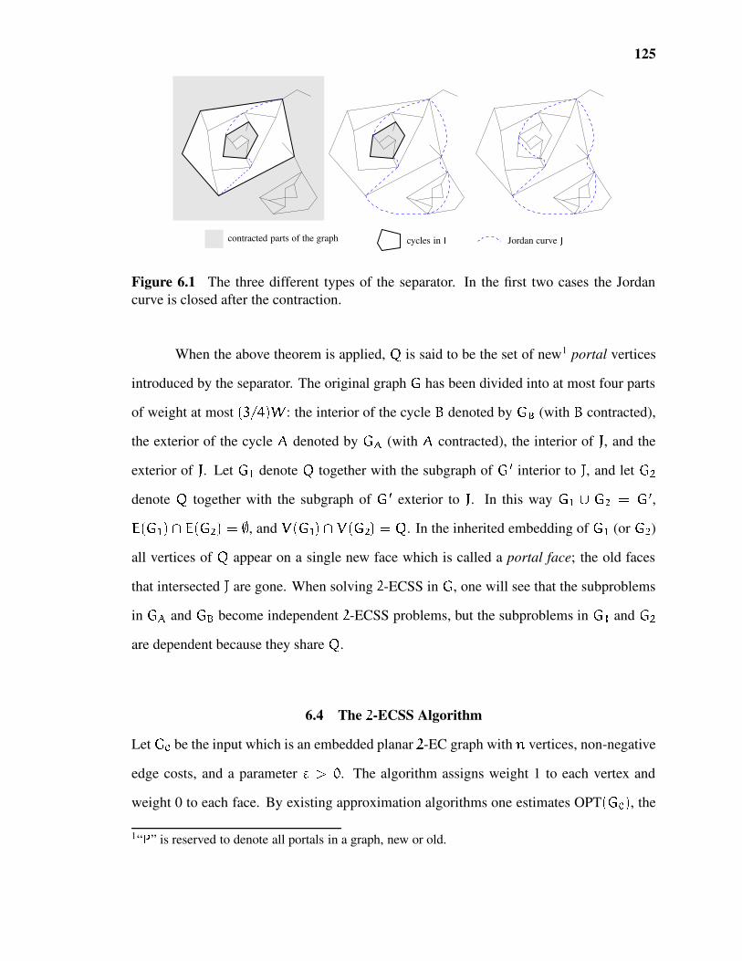
125

contracted parts of the graph Jordan curve @cycles in AFigure 6.1 The three different types of the separator. In the first two cases the Jordancurve is closed after the contraction.

When the above theorem is applied, ) is said to be the set of new1 portal vertices

introduced by the separator. The original graph

has been divided into at most four parts

of weight at most ¶º^Î = : the interior of the cycle È denoted by

CB(with È contracted),

the exterior of the cycle ¨ denoted by-D

(with ¨ contracted), the interior of#, and the

exterior of#. Let

/ denote ) together with the subgraph of interior to

#, and let

1denote ) together with the subgraph of

exterior to#. In this way

/ È 1 ,é: / 5 é< 1 -6, and

b< / 5 D: 1 - ) . In the inherited embedding of / (or

1 )all vertices of ) appear on a single new face which is called a portal face; the old faces

that intersected#

are gone. When solving -ECSS in

, one will see that the subproblems

inED

andFB

become independent -ECSS problems, but the subproblems in / and

1are dependent because they share ) .

6.4 The -ECSS Algorithm

LetRP

be the input which is an embedded planar -EC graph with vertices, non-negative

edge costs, and a parameter uv 9 . The algorithm assigns weight 1 to each vertex and

weight 0 to each face. By existing approximation algorithms one estimates OPT<NP^

, the

1“ ” is reserved to denote all portals in a graph, new or old.

126

minimum cost of a -ECSS, within a constant factor. Fix an integer = Òý² 4´u log ,where 4 U <õPL OPT

<RP^.

A rooted decomposition tree is built fromQP

as follows. Each node of stores

an embedded planar graph

, which has edge costs, vertex/face weights, and some distin-

guished subsetO

of “portal” vertices. The root of storesP

itself, with no portals. Each

node of has at most four children, defined inductively as follows.

Let

be the graph stored at a node of , and let = be its total vertex/face weight.

If = is ¤ = 1 , then this node is a leaf of . Otherwise, apply Theorem 6.3.3 to partition

into at most four pieces (interior of È and exterior of ¨ , and / , 1 ), each of total weight at

most ¶º^Î = . Uncontracted portal vertices from

remain as portals in each piece where

they appear; the graphs / and

1 each get at most = new portals, the set ) . In / and

1 ,assign a weight of = <3 ¼à= to each new portal, and weight =û 3 ¼ to the new portal face.

By the Separator Theorem, the number of new portals obtained in this phase is at most = ,

thus the weight of each of / and

1 is at most ³ = x = è< // M ' = x // M = KG = . In the graphDand

FB, assign the new (non-portal) vertex weight

3and all the the remaining vertices

have the same weight as in

. Since each child has weight at most constant fraction of the

weight of the parent, the tree has depth ¤ log and size ¤ log . Furthermore, ifõPis 2-edge connected, by the separator properties, each

in is

2 N + PO´ -safe.

By the construction,O

is the set of portals in

which have been introduced by some

Jordan cut but not yet cut off by a cycle contraction or another Jordan cut. Now, consider

the number of portals and faces of the smaller graphs. SinceFD

andFB

do not have new

portals and portal faces, one needs consider / and

1 only. The construction ensures that

the portals that / and

1 inherited from

are always heavier than the new portals in the

vertices of#, and the inherited portal faces are always heavier than the new portal face.

This implies that in / and

1 , every portal has weight at least // M ' = , and every portal face

has weight at least // M = . Since / and

1 each has weight at most KG = , one can conclude

that / and

1 each contains at most3 Î= portals and at most

3 ¶ portal faces. Each portal

127

face contains a hole made by a Jordan cut at some ancestor of

in . Note that a Jordan

cut might cut (simply) across an existing portal face, in which case some old portals may

appear on the new portal face, but this still counts as a single portal face. Or in terms of an

embedding on a sphere with holes, all old holes crossed by the Jordan cut disappear, with

segments of their boundaries incorporated into the one new hole boundary.is connected via

Oto the rest of

QP(really a pinched and contracted version ofõP

) which can be embedded as disjoint pieces, one in each portal face of

. Therefore the2 N + POé -type imposed on

Oby the rest of

QPdecomposes into independent types, one

in each portal face of

. By applying Lemma 6.2.4 to each portal face, one may bound and

enumerate the Ü ãH: #<: æ Ü ã 3 ¼ s<æ different2 N + PO´ -types that may be imposed on

Oby

the rest ofõP

. Call this list the list of external types for

. It is more efficient, although not

essential, if each external type of

is represented as a planar graph of size ¤ O (see

Lemma 6.2.3) embedded in the portal faces of

. In particular at the root of the input

graphõP

has no portals, and therefore it has the “empty” external type P .Having computed and these external type lists, one may now define a set of

subproblems that need to be approximately solved:

Definition 6.4.1 For

in (with portal setO

) and an external type for

, the subprob-

lem<( is this: find a min-cost

2 N + PO´ -safe spanning subgraph R of

which is

compatible with , or else declare that<( is infeasible (no such R ).

Checking feasibility is simple: just check whether is compatible with

itself. The to-

tal number of subproblems (over all choices of

and ) is Ü ã 3 ¼ s<æ , and the subproblem:RP° PL is the original -ECSS problem. The subproblems will be approximately solved

starting at the leaves of and finishing at the root. Using dynamic programming, the

solutions are stored to avoid recomputation.

In the base case,

is a leaf of and has sizek ¤ = 1 . Then enumerative

method can be applied based on Lipton-Tarjan separators [85] to exactly solve such sub-

128

problems in Ü ãJI K æ Ü ã 3 ¼ s<æ time (this may be regarded as a continuation of our method,

using Jordan cuts without cycle contractions).

Otherwise

is not a leaf, and has up to four children in as found by Theo-

rem 6.3.3. The external type is decomposed into independent external types, one for each

portal face of

.

Let E denote either

EDorFB

and let E be the subtype of induced by the portal

faces of E . Lookup the solution R E to the subproblem

< E E and lift the edges of R Eand the edges of + to be part of the approximate solution R for the

<( subproblem.

Now consider the two remaining children / and

1 . As in Theorem 6.3.3, let

be what is left of

after the (up to two) cycles are contracted and their interior or exterior

is pinched; so / ÈC 1 . Let 4 denote the external type induced by in the portal

faces of . Not knowing the optimal choice of external types / and 1 for

/ and 1 ,

one needs to try them all. That is, for every pair à/ 1 where subproblems

< / ^/ and: 1 1 were found feasible, one lookups their solutions Rz/ and R©1 and check whether

R RÑ/ È R©1 is compatible with 1 . The cheapest compatible R found are taken, and its

edges are lifted back to

. These edges of R , together with the + and R E edges mentioned

earlier, comprise the approximate solution R for the<( -subproblem.

Although is not actually associated with a node of , note that one can still

speak sensibly of the< 4 subproblem as defined above. In fact it would be a simple

matter to reformulate as a binary tree including : at each internal node of one would

either pinch one cycle, or apply a Jordan cut.

Analysis The above algorithm solves Ü ã 3 ¼ s<æ subproblems, each in Ü ã 3 ¼ s<æ time, so the

total running time is Ü ã 3 ¼ s<æ .Consider a feasible subproblem

<( . By planarity, decomposes into indepen-

dent types in each portal face, and these faces cannot cross a cycle; therefore each cycle-

pinched subproblem: E E and the remaining subproblem

: 4 are all feasible. Tak-

129

ing the external type on / induced by

1 È 4 as °/ , we see that: / °/ is feasible. Sup-

posing (by induction) that the algorithm found some solution R²/ for: / ^/ , then RÑ/ È

induces an external type 1 on 1 such that

: 1 1 is also feasible. Therefore by induction

up , the algorithm finds some solution for each feasible:) -subproblem.

Now suppose R is the solution that the algorithm finds for a feasible subproblem:) . Define the error on<( as the difference between the cost U R and the minimum

possible cost. For each pinched cycle + (up to two), by Facts 6.3.1 and 6.3.2 subproblem:) will inherit the error of< E E plus an additional additive error of at most U + .

After pinching cycles, the remaining error of<( is that from

: 4 . Recall / Èû 1 ; let R T be the unknown optimal solution for: . Let T / denote the

external type of / induced by

R)TL5 1 È 4 , and similarly let T1 denote the external type

of 1 induced by

R)T-5 / ÝÈ 4 . Then< ¥ T¥ has the optimal solution RT-5 ¥ (for¦£ 3" ), and

T / T1 is a compatible type pair considered by the algorithm; if these two

subproblems are solved optimally, the solution cost would be U R T . Therefore the error

on< 4 is at most the sum of the errors on

< / T / and< 1 T1 , even though one might

not actually find the best solution R using this pair. Therefore error terms simply add at a

Jordan cut.

Therefore the total error of the root problem<QP° P is at most the sum of U +

over all cycles contracted in . It is easy to see that for any level of , the total edge cost

of that level is at most U <RP^ . Therefore the total edge cost of all cycles contracted on that

level is ¤ U <RP^ à= . Summing over all ¤ log levels of , the total error from all levels

of is ¤ U <RP à= log . By an appropriate choice of the leading constant defining = ,

this is at most u è OPT<RP^

. Therefore the final solution has cost at most<3[x u OPT

<P^,

proving Theorem 6.1.1.

130

6.5 The -VCSS Algorithm

The main idea of the -VCSS algorithm is similar to the -ECSS algorithm. Given the

input plane graphQP

, the separator theorem is applied to decomposeP

hierarchically into

small pieces. For each piece, types are used to enumerate the different ways that the “rest”

of the graph may influence the connectivity constraints within this piece. Then, dynamic

programming is used to approximately find the minimum subgraph compatible for each

type of each piece. Similarly one can prove that the number of external types of each

piece is a simple exponential in the number of portals (Lemma 6.5.4), yielding the same

running time analysis. Again the only source of error is in the weight of the separating

cycle edges, yielding the same error analysis.

However, there are some difficulties preventing one from using the same technique

to solve the -VCSS problem. The principle difficulty is cycle contraction. In the -ECSS

algorithm, the decomposition, type definition and dynamic programming are all performed

on the minors ofRP

, and it is shown that this is sufficient. But it is no longer reasonable to

contract the cycles in the -VCSS problem, because this changes the problem (in particular,

it may introduce a false cutvertex). Therefore for each node in , a pair of graphs are kept,

the compressed subgraph

as defined in the -ECSS algorithm and its corresponding

uncompressed subgraph M , that is the subgraph ofP

induced by all vertices which appear

(after cycle contractions) as some vertex in

. As before, the separator theorem is still

applied to

, and the decomposition of M is obtained naturally. But the type and dynamic

programming will be defined on M .

The uncompressed graph M also contains portal vertices and portal faces, which are

the preimages of the portals and portal faces in

. Specifically, let#

be the Jordan cut when

the separator theorem is applied to

. Let · be a vertex on#. If · is mapped to a single

vertex of M , then · is a new portal that will be contained in the subgraphs of M . Otherwise,

· is mapped to many vertices which are on a series of cycles in M , then at most of these

vertices will be specified as new portals of M . These two vertices are where the Jordan cut#

131

would intersect M if the cycles represented by · are uncontracted. Thus there are still ¤ = portals in M . Each portal appears on some portal face in M corresponding to the portal faces

of

, and the portal faces identify where “the rest ofP

” would appear in the embedding.

The edges of each separating cycle will appear in M as hard edges which are committed to

the final solution as in the -ECSS algorithm.

The notion of types must also be redeveloped in the biconnected context, so that one

may again use types to characterize the possible counterparts of an uncompressed graph;

this is the point of Lemma 6.5.2 below. For convenience, types are simply represented as

graphs (rather than abstract cut tables represented by graphs, as in Section 6.2). Following

is a definition analogous to “k N + PO´ -safe” graphs.

Definition 6.5.1 For a graph ë P

with a portal setO µ

, a graph R ë P

is called a counterpart (of

) if 5 µ O

. The graphÈ R is obtained

by taking the union of the vertices and edges of the

and R and keeping the multiplicity

of each vertex and edge at most3. The graph

is called

2 N + O- -safe if it has a

counterpart R such that È R is biconnected.

6.5.1 Types of ( -VC, P)-Safe Planar Graphs

The type of a2 N + PO -safe graph is a graph describing a simplified characterization of

the biconnectivity information of the portals in the graph.

Definition of the type. The definition of type is operational and it is oriented towards

Lemmas 6.5.2 and 6.5.4 below. Let R P be any

2 N + O -safe graph (does

not have to be planar) with a distinguished portal setO

and a distinguished set of hard

edges ã . The type R of R is defined by performing a series of operations on R . See

Figure 6.2 for an illustration.

132

1. Let R ã be the graph consisting all portals ofO

and all the edges of ã . From R ã ,

construct a simplified graph R ã which is a forest formed by a collection of (possibly

connected) stars2:

(a) All vertices of R ã are included in R ã .(b) Every portal of

Ois marked as a super-portal.

(c) For each vertex À O , if it is a cutvertex or an end vertex of an isolated edge

in R ã , mark it as a super-portal in R ã .(d) For each block of R ã (hard block) with at least two vertices, create a new vertex

in R ã as a super-portal and connect by an edge the super-portal to every vertex

in the block.

(e) Assign distinct IDs to all super-portals.

2. Replace the subgraph R ã of R by the graph R ã and remove those vertices that have

no ID and are adjacent only to a super-portal (notice that the removed vertices are all

connected only to vertices of a hard block of R ã ). Let the obtained graph be R .

3. For each block of R that is not a bridge, if it has exactly two cutvertices and does not

contain a super-portal, contract it into a single vertex.

4. Repeat the following two operations until none apply.

(a) Remove all chords in any cycle of R .

(b) For each path of R with no super-portals as internal vertices and all internal

vertices with degree exactly , contract to an edge with the same end vertices

as .

2Notice a similarity of this construction to the standard construction of cutvertex-trees, see, e.g.,[32].

133

5. Let R be the graph obtained after Steps 1–4. The type R is a graph with some

vertices labeled (having IDs, these are vertices corresponding to super-portals and

will be called portal nodes). It is constructed from R as follows:

(a) Add each cutvertex Ê in R to R , and refer to Ê as a cutvertex in R . If it

is a super-portal · in R , then it is a portal-node in R with the ID of · .

(b) For each block in R that does not contain any super-portals, contract it to a

vertex in R . This vertex in R is referred as a block-vertex.

(c) For each block in R containing exactly one super-portal · , contract this block

to a block-vertex. If the block is not a bridge and · is not a cutvertex in R ,then this block-vertex is a portal node in R with the ID of · .

(d) Connect a block-vertex by an edge in R to each cutvertex adjacent to it or to

the endvertices of the bridge if the block-vertex is obtained from the bridge in

R .(e) If a block has two or more super-portals, then keep the block in R as it is in

R .(f) Finally, for each path of R with no portal-nodes as internal vertices and

all internal vertices with degree exactly , contract to a single edge with the

same end vertices as .

Note the concept of super-portal can be applied to any graph R that contains portals

and hard edges, and it is completely determined by the portal set and the hard edge set of

R .

Properties of the types. Some basic properties of the types are listed here. First of all,

the number of labels of R is identical to the number of super-portals of R . Secondly,

notice that the type R is uniquely defined. Let Rm/ and R©1 be two2 N + PO -safe graphs

on the same vertex set and with the same set of portals and hard edges. Then R²/ and R©1

134

are said to have the same type if R/ and R©1 are identical with respect to their IDs.

Thirdly, all vertices that are not portal-nodes have degree at least ¶ . Next, notice that if

R is biconnected and the portal set and hard edges are empty, then R contains a single

vertex (block-vertex). Finally, it is easy to see that the connections among portals in R are

preserved and presenteed by the connections of portal nodes in R . These properties can

be summarized in the following lemma.

Lemma 6.5.2 Let

and R be two2 N + O -safe graphs that have the same set of portalsO

and the same set of hard edges-ã

. Let R be the type of R . Then for any spanning

subgraph of

that contains all hard edges in

-ã, < and R have the same set of

portal-nodes with respect to IDs, and È R is biconnected if and only if < +È R is

-edge connected and the cutvertices of : È R are block-vertices of R or < or the super-portals resulting from contractions of hard blocks as defined in the type.

Let R be a counterpart of

with the same set of portals and hard edges, ifiÈ R is

biconnected, then

is said to be compatible with R . To check whether

is compatible

with R , by the above lemma, it is enough to check whether <£8È R is -edge

connected and the cutvertices of :(+È R are block-vertices of <£ or R or super-

portals representing hard blocks of

and R .

Next, the number of types, specifically, the number of external types of2 N + O -

safe plane graphs is considered. Let

be a2 N + PO -safe plane graph with a hard edge

set|ã

and a portal face set Á . Let the super-portal set of

determined byO

and*ã

beOON

.

If R be a counterpart of

that can be embedded in Á , 3 then the type R of R is said to

be an external type of

with respect to Á . The focus will be on the counterpart R of

that also is2 N + O -safe and shares the same set of super-portals

OPN(i.e., R and

have

the same set of portals and hard edges). Then, the type R is called an external type of

with respect toOQN

and Á . The goal is to show that the number of external types of

with

3That is, is drawn on the plane such that all vertices and edges of are contained in the portalfaces Z (including the boundaries of all faces in Z ).

135

respect toOQN

and Á is small, that is, it is only exponential in OPN . The following lemma

shows a type of a plane graph R can always maintain some topology of R .

Lemma 6.5.3 Let R ë6be a planar graph with a set of portals

O µ that is

embedded on the plane. Then, one can draw R on the plane such that R is planar

and each portal node of R is drawn at the same location as one 4 of the corresponding

portals in R .

Proof : Every single operation performed on R while constructing R satisfies this

property, and hence any sequence of such operations satisfies it too. áFollowing is the the main lemma bounding the number of types.

Lemma 6.5.4 LetÄ P

be a2 N + PO -safe plane graph with a hard edge set|ã

, a super-portal setOQN

and a portal face set Á . is embedded in a way such that all

super-portals ofOQN

will be on the border of the portal faces if the graphQã

consisting of all

portals and hard edges is replaced with Íã as in the definition of type. Then the number of

external types of

with respect toORN

and Á induced by2 N + PO -safe graphs is at most

º ã;: #TSU: æ .Proof : Let R be any

2 N + PO -safe plane graph that has super-portal set

Oand is

embedded in Á . For each portal face Áà¥ , let the subgraph of R embedded in Áà¥ be R©¥ .Because R is plane, R©¥ is disjoint with R(, for

¦Dj | . Correspondingly, the subgraphs of

R in different faces are also disjoint. Hence the type of the subgraph in each face can be

considered independently.

Fix any face Á±¥AßÁ and the subgraph R£¥ of R in Á°¥ . Let its type be ¥ . Now consider

the structure of ¥ . The vertices in ¥ whose degree is at most one are going to be called as

leaves. A leaf must be a portal node ofO

, because all vertices that are not portal nodes have

degree at least ¶ by the construction of R . Secondly, there may be some parallel edges

4A portal node in VLaW e may corresponds to many portals because the hard edges are compressed.

136

in ¥ which must be between two portal nodes (super-portals), because otherwise it will be

contracted according to Step 4a-4b of the definition. If ¥ contains a block, then the block

must be a cycle. This is because by assumption and Lemma 6.5.3, all portal nodes are on

the boundary of Á±¥ , thus can not be inside a block. But after Step 1-3, no vertex will remain

inside the cycle. Furthermore, by construction of ¥ , each such cycle in ¥ contains at least

two portal nodes and all non-portal vertices on the cycle must have degree at least ¶ .For the purpose of counting, one can transform ¥ into a forest with only bÕO ¥

leaves. If one erases each portal node and an infinitesimal neighborhood around it, then a

forest will be obtained with all internal nodes have degree at least ¶ with no ID assigned.

The leaves correspond to portals-nodes, they have the same ID as the corresponding portal-

nodes. It can be claimed that the number of the leaves isDÕO ¥ 5. Thus, there are at most

º ã;: # Ó : æ such forests.

Hence, the number of types ¥ in face Á°¥ is proved to be º ãH: # Ó : æ . Because ¥ and ,are independent for

¦(j | , the total number of possible external types with respect toO

and

Á is ?YX Z[XÓ C 1 ½ ¿ X \ Ó X Â . This completes the proof. áLet

W] R be a pair stored in a node of where]

is the uncompressed2 N + O -

safe graph. Suppose]

has a portal setO

and a hard edge setã

. Let be an external type

of]

.]

is said to be compatible with if W])ÅÈ is -edge connected and the cutvertices

of W])ÅÈ are block-vertices of W]( or or super-portals representing hard blocks.

By Lemma 6.5.4, the number of possible external types is determined by the number

of super-portals of]

. Now it will be shown that the number of super-portals in each

subgraph obtained from separator theorem isb = . By definition, the number of super-

portals of]

is at most the number of portals in it plus the number of separating cycles (hard

cycles) and the cutvertices between these cycles. Because the depth of the decomposition

5The operation can be seen as two steps. First break the cycles at the portals on the cycle by erasingonly the neighborhood on the cycle edge. Thus one gets at most ñ_^ ¥`^ new leaves, and the obtainedgraph is a forest with internal vertices degree at least three except those portal nodes. Therefore, thenumber of edges of the forest is fgaU^ ¥a^ e . To make all portal nodes be leaves, one can do the sameoperation to the internal portal nodes and gets the final forest.

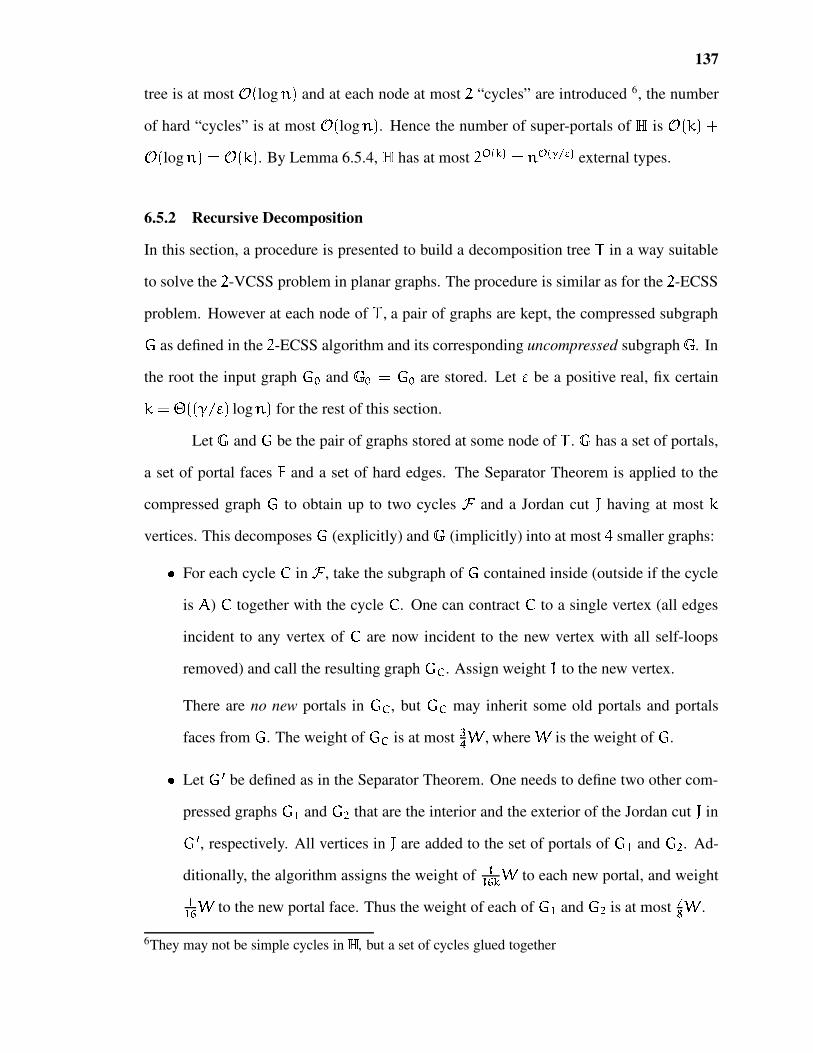
137

tree is at mostD

log and at each node at most “cycles” are introduced 6, the number

of hard “cycles” is at mostb

log . Hence the number of super-portals of]

isD = xb

log KD = . By Lemma 6.5.4,]

has at most Ü ã 'æ º ã 3 ¼ s<æ external types.

6.5.2 Recursive Decomposition

In this section, a procedure is presented to build a decomposition tree¢

in a way suitable

to solve the -VCSS problem in planar graphs. The procedure is similar as for the -ECSS

problem. However at each node of¢

, a pair of graphs are kept, the compressed subgraphas defined in the -ECSS algorithm and its corresponding uncompressed subgraph M . In

the root the input graphQP

and M Pb õPare stored. Let u be a positive real, fix certain

= ý² 4éu log for the rest of this section.

Let M and

be the pair of graphs stored at some node of¢

. M has a set of portals,

a set of portal faces Á and a set of hard edges. The Separator Theorem is applied to the

compressed graph

to obtain up to two cycles b and a Jordan cut#

having at most =vertices. This decomposes

(explicitly) and M (implicitly) into at most Î smaller graphs:

For each cycle + in b , take the subgraph of

contained inside (outside if the cycle

is ¨ ) + together with the cycle + . One can contract + to a single vertex (all edges

incident to any vertex of + are now incident to the new vertex with all self-loops

removed) and call the resulting graph E . Assign weight

3to the new vertex.

There are no new portals in E , but

E may inherit some old portals and portals

faces from

. The weight of E is at most ³ = , where = is the weight of

.

Let be defined as in the Separator Theorem. One needs to define two other com-

pressed graphs / and

1 that are the interior and the exterior of the Jordan cut#

in , respectively. All vertices in#

are added to the set of portals of / and

1 . Ad-

ditionally, the algorithm assigns the weight of // M ' = to each new portal, and weight// M = to the new portal face. Thus the weight of each of / and

1 is at most KG = .

6They may not be simple cycles in c , but a set of cycles glued together

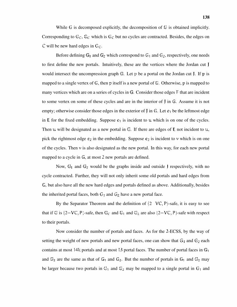
138

While

is decomposed explicitly, the decomposition of M is obtained implicitly.

Corresponding to E , M E which is

E but no cycles are contracted. Besides, the edges on

+ will be new hard edges in E .

Before defining M£/ and M61 which correspond to / and

1 , respectively, one needs

to first define the new portals. Intuitively, these are the vertices where the Jordan cut#

would intersect the uncompression graph M . Let · be a portal on the Jordan cut#. If · is

mapped to a single vertex of

, then · itself is a new portal of M . Otherwise, · is mapped to

many vertices which are on a series of cycles in M . Consider those edges

that are incident

to some vertex on some of these cycles and are in the interior of#

in

. Assume it is not

empty; otherwise consider those edges in the exterior of#

in

. Let S/ be the leftmost edge

in

for the fixed embedding. Suppose Sº/ is incident to which is on one of the cycles.

Then will be designated as a new portal in M . If there are edges of

not incident to ,

pick the rightmost edge SL1 in the embedding. Suppose SL1 is incident to which is on one

of the cycles. Then is also designated as the new portal. In this way, for each new portal

mapped to a cycle in

, at most new portals are defined.

Now, M7/ and M61 would be the graphs inside and outside#

respectively, with no

cycle contracted. Further, they will not only inherit some old portals and hard edges from

M , but also have all the new hard edges and portals defined as above. Additionally, besides

the inherited portal faces, both / and

1 have a new portal face.

By the Separator Theorem and the definition of2 N + O -safe, it is easy to see

that if M is2 N + O -safe, then M E and M©/ and MH1 are also

2 N + PO -safe with respect

to their portals.

Now consider the number of portals and faces. As for the -ECSS, by the way of

setting the weight of new portals and new portal faces, one can show that / and

1 each

contains at most3 Î= portals and at most

3 ¶ portal faces. The number of portal faces in M)/and MH1 are the same as that of

/ and 1 . But the number of portals in M£/ and M1 may

be larger because two portals in M)/ and MH1 may be mapped to a single portal in / and

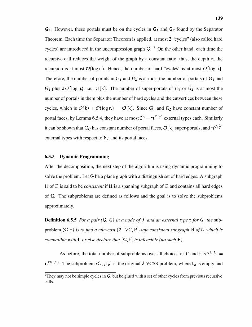
139 1 . However, these portals must be on the cycles in / and

1 found by the Separator

Theorem. Each time the Separator Theorem is applied, at most “cycles” (also called hard

cycles) are introduced in the uncompression graph

. 7 On the other hand, each time the

recursive call reduces the weight of the graph by a constant ratio, thus, the depth of the

recursion is at mostb

log . Hence, the number of hard “cycles” is at mostb

log .Therefore, the number of portals in M)/ and M61 is at most the number of portals of

/ and 1 plus D log , i.e.,b = . The number of super-portals of M(/ or M61 is at most the

number of portals in them plus the number of hard cycles and the cutvertices between these

cycles, which isb = Íxúb log ¿ÜD = . Since M£/ and MH1 have constant number of

portal faces, by Lemma 6.5.4, they have at most ' º ã d æ external types each. Similarly

it can be shown that E has constant number of portal faces,

b = super-portals, and º ã d æexternal types with respect to

O E and its portal faces.

6.5.3 Dynamic Programming

After the decomposition, the next step of the algorithm is using dynamic programming to

solve the problem. Let M be a plane graph with a distinguish set of hard edges. A subgraph]of M is said to be consistent if

]is a spanning subgraph of M and contains all hard edges

of M . The subproblems are defined as follows and the goal is to solve the subproblems

approximately.

Definition 6.5.5 For a pair (

, M ) in a node of and an external type for M , the sub-

problem M is to find a min-cost

2 N + PO -safe consistent subgraph

]of M which is

compatible with , or else declare that M is infeasible (no such

]).

As before, the total number of subproblems over all choices of M and is Ü ã 'æ º ã 3 ¼ s<æ . The subproblem

M P PL is the original -VCSS problem, where P is empty and

7They may not be simple cycles in ' , but be glued with a set of other cycles from previous recursivecalls.

140õPis the input graph with no portals and no hard edges. Each vertex in

Phas weight

3,

each face and edge has weight 9 .As for the -ECSS problem, the problems associated with the leaves where the

compressed

has sizek ¤ = 1 are considered first. All hard edges of M are included

in the solution to M . The subproblem instance are solved exactly in Ü ã I K æ Ü ã 3 ¼ s<æ

time by applying Lipton-Tarjon Theorem [85] to

(explicitly) and M (implicitly).

Let M be a subproblem associated with an internal node of

¢based on the

solutions to the subproblems associated with the children nodes. Suppose the problem

instance for the children of M , M D , M B , M7/ and M61 , have been solved.

Let E represent either

EDoreB

. Let + be the subgraph of that is induced by

the super-portals of M E . The minimum subgraph] E of M E compatible with type + can

be found by looking up the solution to the problem instance of M E .

Let £Nl + . The solution] to

M can be found by combining the

solutions to M©/ °/ and

M1 1 where ^/ È 1 . Then,] E Èf] is approximately the

minimum consistent subgraph of

for external type .Analysis of the algorithm As the algorithm for -ECSS, the only source of error comes

from the cycles in the the separator, i.e., the hard edges. Using similar analysis, one can

show that by selecting an appropriate constant in = ý² 4´u Og , the error is at most

u times the optimal.

For the time complexity, the time spent in the decomposition phase is mainly for

the run of the Separator Theorem which is applied at mostD log times, so the total

time isD 1 log . In the dynamic programming, there are º ã 3 ¼ s<æ subproblems, each

can be solved in º ã 3 ¼ s<æ time. So, the running time for the whole algorithm is º ã 3 ¼ s<æ .This proves Theorem 6.1.2.

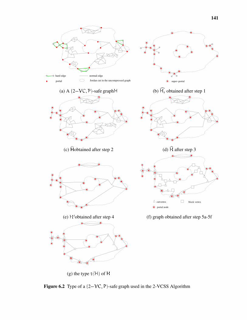
141

Jordan cut in the uncompressed graphportal

normal edgehard edge

super−portal

(a) A2 N + O[ -safe graph R (b) R ã obtained after step 1

(c) R obtained after step 2 (d) R after step 3

block vertex

portal node

cutvertex

(e) R obtained after step 4 (f) graph obtained after step 5a-5f

(g) the type R of RFigure 6.2 Type of a

2 N + O -safe graph used in the 2-VCSS Algorithm

CHAPTER 7

APPROXIMATION SCHEMES FOR MINIMUM 2-CONNECTED SPANNING

SUBGRAPHS IN WEIGHTED PLANAR GRAPHS

7.1 Introduction

In this chapter the approximation algorithms for the -ECSS and -VCSS problem in ar-

bitrary weighted planar graphs are studied. A standard relaxation of the 2-ECSS prob-

lem is also considered which is to find a minimum weight 2-EC spanning sub-multigraph

(2-ECSSM) R of

, meaning that an edge of

can be used multiple times in R (conse-

quently its weight is also counted multiple times in R ). Another classical extension is the

1-2-connectivity problem: each vertex is assigned a connectivity type ßû8 3" "; . The

problem is to find a minimum weight spanning subgraph such that for any pair of vertices

, there are at least min8i P; edge-disjoint or vertex-disjoint paths between

and . The 1-2-edge-connectivity is denoted by h 1,2 i -EC, and 1-2-vertex-connectivity

by h 1,2 i -VC. The relaxed 1-2-edge-connectivity problem where each edge may be used

more than once is also considered.

7.1.1 Related Results

All the problems mentioned above have been extensively studied in the literature. Since all

these problems are ÉÊ -hard, the main research has been devoted to designing efficient ap-

proximation algorithms, see the survey [70] and more recent advances [19, 39, 40, 66, 74].

In general, one would prefer to design a PTAS. However, all the problems considered in

this chapter are max-SNP-hard [25]. Therefore they do not have a PTAS unless Ê ÉÊ .

But this does not preclude a PTAS for restricted classes of graphs: indeed, in the previous

chapter, it has been shown that there are PTASs for both 2-ECSS and 2-VCSS problems

in unweighted planar graphs as. In fact, the approximation schemes of in Chapter 6 al-

low weighted planar graphs, but then the algorithms will either run in time Ükjl ã æs"éOPT m to

142

143

ensure an<3Íx u -approximate solution or they run in polynomial time with an approxima-

tion guarantee of 1+ ¤ l ã æs"é OPT

. Since the ratio <£ OPT could be arbitrarily large, these

algorithms are in general not PTAS’s for weighted planar graphs.

For both the 2-ECSS and 2-VCSS problems in weighted planar graphs, the best

known polynomial-time or even quasi-polynomial-time approximation guarantee is still 2

[73, 94], which is achieved by polynomial-time algorithms working for general weigh-

ted graphs. The best known result for h 1,2 i -ECSS in weighted planar graphs is a 2-

approximation algorithm, due to Jain [64], which in fact solves the more general problem

where = for any = . For the weighted h 1,2 i -VCSS problem, Fleischer [36] gives a 2-

approximation algorithm, which actually solves the h 0,1,2 i -VCSS problem. A PTAS for

the geometric version of these problems is presented in [27].

7.1.2 New Contributions and Techniques

Efficient approximation schemes for all the above mentioned problems in weighted planar

graphs will be presented. These approximation algorithms depend in a crucial way on the

new construction of light spanners for planar graphs.

Let

be a weighted graph. LetÅ denote the weighted shortest path distance

between the vertices and in

. An ß -spanner of

is a spanning subgraph R of

such

that [ ß è for all . A spanner provides an approximate representation

of the shortest path metric (1-connectivity) in

, but it may be much lighter than

.

Althofer et al. [1] designed a simple greedy algorithm that for an arbitrary graph

computes an ß -spanner R of

for any ß(v 3 . In the case of planar graphs, it is shown in [1]

that this spanner has weight R [ :3°x ßLN 3 ¡ X¢ <£ , where¡ X¢ :(

is the weight

of a minimum spanning tree in

. Since¡ X¢ <£W

OPT for all the problems considered,

this bounds the ratio R OPT in terms of just ß . If all weighted graphs in a graph

family have spanners with such a bound on R OPT (depending only on ß ), then the

family is said to have light spanners for this problem. Light spanners are known to be very

144

useful for solving various optimization problems on graphs. For example, planar graphs

have light spanners for metric-TSP: the first step in the metric-TSP PTAS for weighted

planar graphs [4] is to replace the input graph with an accurate enough ß -spanner (using

[1]), thus effectively bounding :( OPT for the remainder of the algorithm. Spanners

are also used in complete geometric graphs to design efficient PTAS’s for geometric TSP

and related problems [101], and to design PTAS’s for the 2-edge and 2-vertex-connectivity

problems [26, 27].

By combining the spanner constructed in [1] with the planar separator decomposi-

tion approach tuned to analyze 2-connected graphs in Chapter 6, it will be shown that one

can design a PTAS for the 2-ECSSM problem and a PTAS for the h 1,2 i -ECSSM problem.

However, this approach of replacing the input graph with an ß -spanner fails for the 2-ECSS

and 2-VCSS problems. The reason is that a spanner does not have to be 2-connected, thus

the spanner may not contain the optimal or a near optimal solution in most cases. Naturally,

one may think to use light fault-tolerant spanners (see, e.g., in [82]), which are subgraphs

that persist as ß -spanners even after deleting a constant number of vertices or edges. Un-

fortunately, this concept is not useful for weighted planar graphs, since simple examples

show that light fault-tolerant spanners do not exist in weighted planar graphs, not even for

a single edge deletion.

To solve the problem mentioned above, the main contribution is described: a new

greedy spanner construction which produces a light planar spanner with certain desirable

properties. Specifically, given a weighted planar graph

, a connected spanning subgraph

¨ of

and ßv 3, it computes an ß -spanner R of

. R contains ¨ as a subgraph and

has total weight R ¤ :3 ß£N 36è ¨ . Thus if the algorithm is fed with n -

approximate solutions R to the various connectivity problems in a weighted planar graph, then an ¤ nK ßÍN 3 -approximation RT for that problem is obtained where R¿T is an ß -

spanner for

at the same time. Furthermore, one can show that while RÑT need not contain

145

an<3Øx u -approximate solution

X, the number of edges of

X“crossing” each face of RÑT

(Lemma 7.4.2) is bounded.

Using the new spanner construction technique and the planar separator decompo-

sition, one can design approximation schemes for the 2-ECSS and 2-VCSS, h 1,2 i -ECSS

and h 1,2 i -VCSS problems, which find solutions with weight at most:3)x u 6è OPT in

Ü ã log ¬ log ã / ¼ s<æ ¼ s<æ time; these are quasi-polynomial time approximation schemes (QPTAS’s).

Organization. First a PTAS for the 2-ECSSM problem is presented in Section 7.2. This

section contains also a description of the main algorithmic approach used in our approxi-

mation schemes, which is a combination of the use of spanners, a recursive approach driven

by a variant of the planar separator theorem, and dynamic programming. Next, in Sections

7.3 and 7.4, the new construction of spanners is described and the special properties of

the spanners are discussed. In Section 7.5, quasi-polynomial approximation schemes for

the 2-ECSS and the 2-VCSS problems are presnted. Finally in Section 7.6, h 1,2 i -ECSS

and h 1,2 i -VCSS problems are considered : a PTAS for the h 1,2 i -ECSSM problem and a

QPTAS for each of the h 1,2 i -ECSS and h 1,2 i -VCSS problems are presented.

7.2 PTAS for the 2-ECSSM Problem

Let

be a connected weighted graph. A 2-ECSSM R of

is a spanning sub-multigraph

of

in which edges can have some multiplicity and in which every pair of vertices is

connected by at least two edge-disjoint paths. Note that

may not have any multiple

edges at all. If an edge is used multiple times in R , its weight also contributes multiple

times to the weight of R . Since it never helps to use an edge more than twice, one may cap

all edge multiplicities at two. Following is a PTAS for this problem which runs in Ü ã / ¼ s ætime.

Given

and u«vÄ9 , the algorithms chooses ß so that ß 1 3(x u . First an ß -spanner R in

is computed by the greedy spanner algorithm [1], with weight R )

146

¤ <3 u è OPT. Now it will be shown that there is a

:36x u -approximate 2-ECSSM that

uses only edges from R . SupposeX T is an optimal 2-ECSSM in

with X T © OPT.

NowX T is modifed such that it uses only edges from R . For each edge S of

X T not in R ,

remove S and add a shortest path from R of total weight at most ß è S . When the path

is added, the edges are added with multiplicity, but capped at two. The result of all these

modifications is another 2-ECSSMX

, using only edges from R , each edge used at most

twice, with X ß è OPT.

Next the algorithm applies the 2-ECSS ß -approximation algorithm from Chapter 6

to the graph Rú , which is R with each edge duplicated. In summary, one can get the

following theorem.

Theorem 7.2.1 Let u£v9 and let

be a connected weighted planar graph with vertices.

There is an algorithm running in time Ü ã / ¼ s æ that outputs a 2-ECSSM of

whose weight

is at most:3x u times the minimum.

Why this technique fails for other problems: The above technique does not work for

other problems considered in this chapter, because in these problems, we are not allowed

to duplicate edges from

in the output graph. Instead, our approximation schemes must

consider the possibility that the near-optimalX

needs some “extra” edges from outside the

spanner. In Sections 7.3 and 7.4 a new type of light planar spanners are developed and the

number and arrangement of those extra edges outside the spanner are limited.

7.3 Augmented Planar Spanners

In this section a new greedy algorithm is presented to construct ß -spanners in weighted

planar graphs, resembling the standard greedy algorithm [1] for general graphs. Just as in

the standard algorithm, the algorithm takes a connected weighted graph

and a parameterßg5 3, and produces an ß -spanner R . Unlike the general algorithm, our

must be planar,

and for each edge S of

not in R it is guaranteed that ß è S is at least the length of

147

f

evu

2P

1P

Figure 7.1 A non-simple face Q in R , a chord S , and walksO / and

O 1 .some path in the face of R containing S . The new algorithm is also provided with a third

argument: a “seed” spanning subgraph ¨ , containing edges that must appear in R . In

Section 7.4 ¨ will be used to enforce some 2-connectivity properties in the spanner.

Suppose

is a weighted plane graph (that is, an embedded planar graph) and R is

a subgraph. A chord S of R is an edge of

not in R . Note that R and S inherit embeddings

from

. For each chord S S is defined to be the length of the shortest walk connecting

the endpoints of S , along the boundary of the face of R containing S .More precisely, if the endpoints of S are disconnected in R , then define S xon

. Otherwise S connects two vertices in a component of R , and S is embedded in some

face Q of this component. The boundary of Q is a cyclic walk of (oriented) edges, with total

weight Q ; note that a cut-edge may appear twice in the boundary (once per orientation),

and its weight would then count twice in Q . Similarly a cut-vertex may appear multiple

times. The edge S splits the boundary sequence into two walksO / and

O 1 , both connecting

the endpoints of S , with ÕO / x BO 1 K Q . Now define S K min ÕO / P ÕO 1

(see Figure 7.1).

Given

, ß , and ¨ as above, R ¨© g .¹Sé <( ß ¨ is computed as follows:

Augment:) ß ¨ :

Rpì¨for all edges S of

in non-decreasing S order do

if S is not in R and ß è S ÏC S then

148

add S to Rreturn R

Note ¨µ R6µ . If ¨ is empty (has all vertices of

but no edges), then this is

like the general greedy spanner algorithm [1], except that replaces&

.

Theorem 7.3.1 Let

be a weighted plane graph, ßv 3, and ¨ a spanning subgraph of

. Then R ¨7 g .0Sé <( ß ¨ is an ß -spanner of

. If ¨ is connected, then R H:3x ßŃ 3Åè ¨ .Proof : To show that R is an ß -spanner it suffices to show that each edge of

is ß -

approximated in R . For S not in R , at the moment it was rejected it must be the case that

S Ø ß è S . Note that S may only decrease after that, so& S $ S $ß è S at the end of the algorithm.

For the second part one needs to show that the weight of all edges in R but not ¨ is

at most ßŃ 3Wè ¨ . Suppose S is such an edge; then S is not a cut edge in R since

¨ is a connected spanning subgraph. Therefore S is bounded by two distinct faces. Let Qbe either face bounding S . First one can claim that Q v <3$x ß [è S . To see this,

consider the last edge S added to Q whose boundary consists of a pathO

plus S . Since S is added to R , one must have ß è S Ï SÚ and SÚ Ø ÕO´ . Adding SÚ to

both sides of ß è SÚ ÏC ÕO´ , and noting S [ SÚ , one gets the claim.

For each face Q of ¨ , let 8 be the set of edges in R crossing the interior of Q .

Since the sum of Q over all faces of ¨ is è ¨ , it suffices to show that B 8 ¿:3 ßN 3è Q . Note that the edges dual to 8 define a tree on the faces of R inside

Q . Orient this dual tree away from some arbitrarily chosen root: now for each Sy 8 , an

adjacent face Q) of R (only the root was not picked) is chosen. For each S 8 it is known

Q, NÑ è S v ßN 3°è S , from the previous paragraph. Summing these inequalities

over all S) 8 , one gets at most Q on the left hand side, and exactly ßŃ 3¯è Õ 8 on

the right. ÕÖ á

149

7.4 Spanners and 2-EC Subgraphs

Suppose a weighted plane 2-EC graph

is given, where the goal is to find an<3©x u -

approximate 2-ECSS. First one can construct an auxiliary subgraph RÑT , as follows:

1. Compute a 2-approximate 2-ECSS ¨ , in polynomial time.

2. Compute R)T ¨7 g .¹Sé <( Ñ ¨ .The constant Ñ here is not critical, just convenient. By Theorem 7.3.1, R T is a 12-

approximate 2-ECSS. Below it will be shown that for every uÇvÞ9 , this RgT has nice in-

tersection properties with some:3éx u -approximate 2-ECSS in

.

Given a face Q in RT , the chords of Q are the edges of

embedded inside this face,

according to

’s embedding. A face-edge S of Q is an abstract edge connecting two vertices

of Q ; unlike a chord, a face-edge is not necessarily an edge of

. (If vertices appear more

than once on Q , one must specify which appearances is the endpoints of S .) The face edge

S is said to crosses a chord U if: U is a chord of the same face Q , their endpoints are distinct

vertex appearances on Q , and they appear in cyclic “ S^US^U ” order around the boundary of Q .Note that S may be embedded inside Q so S intersects only the crossed chords.

SupposeX

is a 2-ECSS in

, and an edge U ofX

is not in R¿T . Then U is a chord

of some face Q of R)T . LetOÅV

be the path in Q connecting the endpoints of U , such that

ÕOÅVg Ñ è U . Then the chord move at U is the following modification ofX

: add

toX

all the edges ofOWV

that were not already inX

, and remove fromX

any chords inside

the cycle U È¹OÅV (see Figure 7.2(a)). Since R T is 2-EC, the cycle has no repeated edges,

and thereforeX

is still a 2-ECSS after the chord move. The chord move is improving if

X decreases; this happens whenever ÕOV (or Ñ è U ) is less than the weight of

the discarded chords. Any non-trivial chord move bringsX

closer to RÑT (in Hamming

distance), thus at most ¤ improving chord moves apply to any given 2-ECSSX

.

150

cPc

f

f3

c4

c5c

1c

2

eu v

c

a

b

Figure 7.2 (a) Face Q of R)T (oval) with chord U , pathOV

(bold), and chords removed fromXby the chord move at U (dotted). (b) Face Q with a face-edge S (dashed) crossed by five

chords fromX

.

Lemma 7.4.1 Let S be a face edge of a face Q in R T andX

be a 2-ECSS of

. Suppose + is

a set of edges ofX

all of which are chords crossing S , Ñ è minV Ô E U v max

V Ô E U ,and no chord in + gives an improving chord move. Then Ã+ Î .

Proof : If not,X

has five chords crossing S as in Figure 7.2(b). But then there is an

improving chord move at U ³ , since the discarded chords (8<U/ U^1P; or 8<U U ô ; ) weigh more

than Ñ è U ³ . áNow one can argue that by accepting a small additive error in the 2-ECSS, one may

assume it has only a small number of chords crossing a given face-edge:

Lemma 7.4.2 Suppose

and R T are as above, ubvÐ9 , X is a 2-ECSS, Q is a face in R T ,and S is a face-edge in Q . Then there exists a 2-ECSS

X such that X ß X [xu è +8 , where +8 is the set of edges of

X that are chords crossing S , +N8 µ X, and

Ã+8 ¤ log<3 u .

Proof : First one can suppose thatX

has no improving chord move at a chord crossing

S , since such a move could only remove some chords crossing S . Let +E8 be the set of

chords inX

crossing S . Arrange +q8 in “left to right” order, according to how they intersect

S . Let U P ú+?8 be the chord with maximum weight. Say that a chord UÇE+k8 is short if

U u è U P Ñ . Now if there are short chords to the left of U P , perform a chord

move at the rightmost one, U . Similarly if there are short chords to the right of U P , perform

151

a chord move at the leftmost one, U ã . X is the result of these (at most) two chord moves;

note that + 8 contains no short chords except possibly U and U ã .Map each non-short chord Ut«+A8 to the real number log

U PL U , a point in

the real interval p 6 9 log<3 u Åx ¶º° . Note that two edges can be mapped to the same

semi-open subinterval of p of length3 ° only if the heavier edge has weight less than Ñ

times that of the lighter edge. By Lemma 7.4.1, at most four edges can be mapped into the

same subinterval of p of length3 ° . This implies Ã+ 8 ¤ log

<3 u .The chord moves in Q increased X by at most Ñ U ºx U ã- u è U PL ,

which is at most u è +N8 . ÕÖ á

Remarks: In the 2-VCSS case, the initial ¨ should be a 2-approximate 2-VCSS, so that

R(T is a 12-approximate 2-VCSS. Then in the chord move the cycle has no repeated vertices,

thereforeX

remains a 2-VCSS after the move. In Lemmas 7.4.1 and 7.4.2, the only proper-

ties of R)T that are needed were that it was 2-EC (or 2-VC), and that G S Ñ è S for each chord S .

7.5 Approximation Schemes for the 2-ECSS and 2-VCSS Problems

In this section it will be shown how to use our new spanner construction to find quasi-

polynomial time approximation schemes for the 2-ECSS and the 2-VCSS problems in

weighted planar graphs. Following is the QPTAS for 2-ECSS problem.

A similar framework as that in the PTAS for 2-ECSSM problem in Section 7.2

is used. But instead of using the spanner constructed as in [1], now one may use the

augmented spanner R T as constructed in Section 7.4.

First Theorem 6.3.3 is applied to RT with = ý²log 6u to decompose RT . How-

ever, different from the PTAS for the 2-ECSSM problem, R¿T may not contain a near-

optimal solution of the 2-ECSS problem. Thus one cannot work on the pieces of R T di-

rectly. Fortunately, Lemma 7.4.2 guarantees that there exists a near-optimal solution with

152

at most ¤ = log<3 u edges crossing the Jordan curve

#. These crossing edges can be

guessed by trying all Ü ã ' log ã / ¼ s<ædæ possibilities. The guessed edges are added to the corre-

sponding pieces, and the vertices of R¿T along#

together with the endpoints of the guessed

edges determine the set of portalsO

for the new pieces. For each possible new piece with

the guessed edges, weights are assigned to the new portals such that each new piece has

cost at most constant fraction of R T and ¤ = portals. Then the new pieces are recursively

decomposed.

As in the PTAS for the 2-ECSSM problem, for each piece edge-connecti-vity types

are defined to describe how these portals may be connected outside one of the pieces in a:3Wx u -approximate solution. The number of types for each piece is Ü ã ' log ã / ¼ s<ædæ , exponen-

tial in the number of portals. Then, dynamic programming is used to solve the subproblems

as before and the cycle edges are committed to the solution.

The approximation scheme for the 2-VCSS problem is similar, and only the differ-

ences are mentioned here: first, R T is redefined as remarked at the end of Section 7.4, and

then vertex-connectivity types are defined using the same techniques as in Chapter 6.

The error of the final solution comes from two sources. First, the edges of the cycles

that arose from the application of the separator theorem to the solution are added. Since

each piece in the decomposition has weight at most constant fraction of its parent weight,

the depth of the recursive calls is ¤ log . As before, the total error per recursive level is

¤ R T à= log , where = ý²log Hu and R T Í ¤ OPT u . By an appropriate

choice of the leading constant defining = , this is at most u° è OPT.

Moreover, each time a face of R¿T (or its pieces) is cut by a Jordan curve, ¤ log<3 u

crossing edges are guessed. If these edges are guessed optimally (they were edges in some

original optimalX T ), then by Lemma 7.4.2 an additive error of at most u° times the weight

of these guessed edges is paid. Summing over the entire assembly of a possible solution,

the total of these errors is at most u° è OPT.

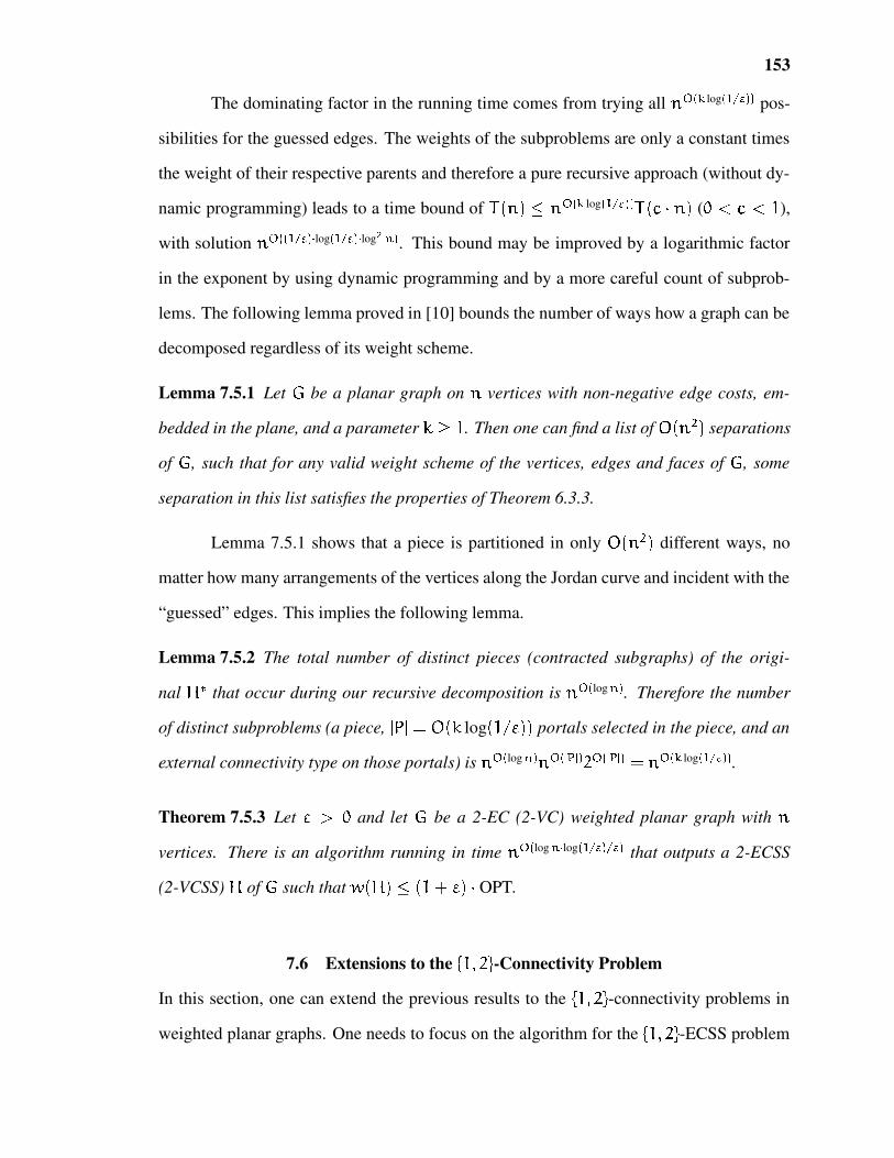
153

The dominating factor in the running time comes from trying all Ü ã ' log ã / ¼ s<æÂæ pos-

sibilities for the guessed edges. The weights of the subproblems are only a constant times

the weight of their respective parents and therefore a pure recursive approach (without dy-

namic programming) leads to a time bound of¢ [ Ü ã ' log ã / ¼ s<æÂæ ¢ U è ( 9Ï U²Ï 3

),

with solution Ü ãÂã / ¼ s<æÁé log ã / ¼ s<æ é log ¬ æ . This bound may be improved by a logarithmic factor

in the exponent by using dynamic programming and by a more careful count of subprob-

lems. The following lemma proved in [10] bounds the number of ways how a graph can be

decomposed regardless of its weight scheme.

Lemma 7.5.1 Let

be a planar graph on vertices with non-negative edge costs, em-

bedded in the plane, and a parameter =b5 3 . Then one can find a list of ¤ 1 separations

of

, such that for any valid weight scheme of the vertices, edges and faces of

, some

separation in this list satisfies the properties of Theorem 6.3.3.

Lemma 7.5.1 shows that a piece is partitioned in only ¤ 1 different ways, no

matter how many arrangements of the vertices along the Jordan curve and incident with the

“guessed” edges. This implies the following lemma.

Lemma 7.5.2 The total number of distinct pieces (contracted subgraphs) of the origi-

nal R)T that occur during our recursive decomposition is Ü ã log ¬ æ . Therefore the number

of distinct subproblems (a piece, O ¤ = log<3 u portals selected in the piece, and an

external connectivity type on those portals) is Ü ã log ¬ æ Ü ã;: #<: æ Ü ã;: #<: æ Ü ã ' log ã / ¼ s<æÂæ .Theorem 7.5.3 Let uvÄ9 and let

be a 2-EC (2-VC) weighted planar graph with

vertices. There is an algorithm running in time Ü ã log ¬ é log ã / ¼ s<æ ¼ s<æ that outputs a 2-ECSS

(2-VCSS) R of

such that R - <3éx u Wè OPT.

7.6 Extensions to the 8 3" "; -Connectivity Problem

In this section, one can extend the previous results to the 8 3" "; -connectivity problems in

weighted planar graphs. One needs to focus on the algorithm for the 8 3" "; -ECSS problem

154

only. The algorithm for the 8 3" "; -VCSS problem can be obtained similarly. The algorithms

presented are modifications of the respective algorithms in Sections 7.2 and 7.5.

First, consider the 8 3" "; -ECSSM problem, which is a relaxed version of the 8 3" "; -ECSS problem where duplicate edges are allowed. As in Section 7.2, it can be shown that

there is a<3$x u -approximate 8 3" "; -ECSSM that uses only edges from a light

<37x u -spanner R . So instead of

, one can work on R with duplicated edges.

The main difference from Section 7.2 is the dynamic programming part. The con-

nectivity types need to be redefined to reflect the non-uniform connectivity requirement.

For this, one can use the connectivity type construction in Chapter 5. Informally, the main

difference is that each time a 2-connected component or path is contracted, the highest

connectivity requirement among all contracted vertices is assigned to the new vertex. This

increases the number of types from Ü ã;: #<: æ to Ü ã 1 : #<: æ , whereO

is the set of portals in the

given graph. Again a PTAS is obtained with running time Ü ã / ¼ s æ .Now consider the 8 3" "; -ECSS problem. First a 2-approximate solution ¨ can be

found using algorithms from [64] (or [36] for 8 3" "; -VCSS). Then ¨ is augmented into a

light spanner R)T as in Section 7.4. Using similar arguments as in the proof of Lemma

7.4.2, one can show that there is a<3£x u -approximate 8 3" "; -ECSS

Xso that for each

picked face-edge S , only ¤ log<3 u edges of

Xcross S . Now redefine the connectivity

types as above. Finally, dynamic programming is used to solve the problem. The running

time is still dominated by the number of subproblems Ü ã log ¬ é log ã / ¼ s<æ ¼ s<æ . Hence, a QPTAS

is obtained in this case.

The results in this section are summarized as follows.

Theorem 7.6.1 Let u¿v9 and let

be a weighted planar graph with vertices. There is

an algorithm running in time Ü ã / ¼ s æ that outputs a h 1,2 i -ECSSM of

whose weight is

at most<3´x u Wè OPT.

155

Theorem 7.6.2 Let u¿v9 and let


an algorithm running in time Ü ã log ¬ é log ã / ¼ s<æ ¼ s<æ that outputs a h 1,2 i -ECSS R of

such that

R - <3x u è OPT.

Theorem 7.6.3 Let u(v9 , and let


an algorithm running in time Ü ã log ¬ é log ã / ¼ s<æ ¼ s<æ that outputs a h 1,2 i -VCSS R of

such that

R - <3x u è OPT.

CHAPTER 8

FAULT-TOLERANT GEOMETRIC SPANNERS

8.1 Introduction

This chapter considers geometric fault-tolerant spanners in Euclidean spaces which are

formally defined as follows.

Definition 8.1.1 (Fault-tolerant spanners [83]) Let

be a set of points in a metric

space, (5 3 a real, and = a non-negative integer. A graphÀíéP

is called a = -vertex

fault-tolerant -spanner for

, denoted by = -VFTS, if for any subset

of

of size at

most = , the graphsr is a -spanner for the point set

tr .Definition 8.1.2 (Edge fault-tolerant spanners [83]) Let

be a set of points in a met-

ric space, 5 3, and = an integer. A graph

Äë6is called a = -edge fault-tolerant

-spanner for

, denoted by = -EFTS, if for any subset

of

of size at most = and for

any pair of points · and in

, the graphur- contains a ·à -path of total length at most

times the length of a shortest path between · and in the graphqv r .

One can show (see [83] and [86]) that a = -VFTS is also a

= -EFTS. There-

fore, from now on, the focus will be on vertex fault-tolerant spanners.

8.1.1 Previous Results

This problem of efficiently constructing good fault tolerant spanners has been proposed

recently by Levcopoulos et al. [83]. They presented in [83] three algorithms constructing = -

vertex fault-tolerant spanners. Their first algorithm is based on the observation that the = x3

-power of a -spanner is a = -VFTS (an ß -power of a graph

is a graph with the same

vertex set as

and it contains an edge between any pair of vertices that are connected by a

path in

with at most ß edges). Therefore, if one starts with the spanner construction from

156

157

[55], then in timeb log Jx ² º ã 'æ one can obtain a

= -VFTS of maximum degree

º ã 'æ and the total cost of º ã 'æ times the cost of a MST. For a constant = , this construction

leads to a fault-tolerant spanner with asymptotically optimal parameters. The other two

algorithms described by Levcopoulos et al. [83] use the well-separated pair decomposition

[13]. It is shown that a = -vertex fault-tolerant spanner can be constructed (i) inD log x

= 1 time withb = 1 edges, or (ii) in

D = log time withb = log edges.

Neither the maximum degree nor the total cost of the fault-tolerant spanner is bounded in

these two algorithms.

In a follow-up paper, Lukovszki [86] gave a construction of = -VFTSs with the

optimal number of edgesb = ; the running time of this algorithm is

D log 0 / xt= log log . Lukovszki presented also a construction of

= -VFTSs with the maxi-

mum degree ofb = 1 and investigated fault-tolerant spanners that allow the use of Steiner

points.

The main idea of that construction in [86] is to take a high-quality (that is, with

constant maximum degree and total cost proportional to the cost of MST, see [5, 55]) -spanner and then put around each point = Steiner points, so that the distance between

the point and any Steiner point associated with it is infinitesimally small. Each point is

connected with all Steiner points associated with it. Furthermore, whenever there is an

edge in the spanner between a pair of input points Ê and T , then this edge is left in our

fault-tolerant spanner and = new edges are created by connecting in a matching the Steiner

points associated with Ê and T . It is not difficult to see that the obtained graph has exactly

=6 additional Steiner points, the degree of each vertex (either input point or a Steiner one)

is upper bounded byb = , and that the total cost of the graph is

D = times the cost of

minimum spanning tree. Furthermore, one can show that if one removes any set of at most

= vertices from that graph, then for any pair of vertices corresponding to the remaining

points there is a path connecting these points whose length is upper bounded by x u times

the Euclidean distance between the points.

158

8.1.2 New Contributions

The main open problem left in [83] and [86] is whether there exist fault-tolerant spanners

having good bounds for the maximum degree and the total cost. The best bounds obtained

in the prior constructions were the = -fault-tolerant spanners having the maximum degree

ofb = 1 by Lukovszki [86], and the one having the total cost of º ã 'æ times the cost of an

MST by Levcopoulos et al. [83].

The first result in this paper resolves that problem and gives a construction of opti-

mal = -VFTSs.

Theorem 8.1.3 Let

be a set of points in M . Let ²v 3and let = be a positive integer.

Then, one can construct a = -VFTS for

that has maximum degree

b = and whose

total cost isD = 1 è = MST

, where = MST denotes the cost an MST of

. The constants implicit

in the

-notation depend on and

.

Notice that by the arguments above this result implies the identical result for = -edge

fault-tolerant spanners.

It is not difficult to see that the spanner promised in Theorem 8.1.3 has asymptot-

ically optimal bounds both for the maximum degree and the total cost. Indeed, since a = -VFTS ( = -EFTS) has to be = xÀ3 -edge connected, every vertex must have degreew = . To see that the total cost must be

w = 1 è = MST

in the worst-case, consider the fol-

lowing construction (see also [83]), see Figure 8.1. Suppose that = is even. Let U&/ and U^1 be

two points with U/îU^1L w3and let yx 3 ^ . Consider points such that =&° of them are

contained in a ball È´/ of radius centered at U/ and the remaining ÇN0=&° points are con-

tained in another ball È1 of radius with the center at U°1 . Since any MST of these points

has only a single edge between Èé/ and ÈW1 , = MST

öb<3. However, since the minimum

degree of any = -vertex (or = -edge) fault-tolerant spanner is = xC3 , every vertex in È6/ has to

be connected to at least =&° x vertices contained in ball ÈÍ1 . Therefore, there arew = 1

edges between È´/ and ÈW1 , and the cost of any = -vertex (or = -edge) fault-tolerant spanner isw = 1 è = MST

.

159

B1B 1 2

k/2 vertices (n−k/2) vertices(kΩ ) edges2

Figure 8.1 Any Y-Z\°] for points in _-/ and _J1 must have weight at least `badc 1 e , while the MSThas weight fgaih e .

The construction in Theorem 8.1.3 is a generalization of the greedy algorithm that

has been used before to construct spanners [1, 5, 15, 30, 55]. The main contribution in this

context is the first, precise analysis of the fault-tolerant spanners obtained in that construc-

tion.

The next contribution gives an efficient construction of good fault-tolerant span-

ners. The construction from Theorem 8.1.3 gives fault-tolerant spanners having optimal

parameters, but it does not lead to an efficient algorithm for constructing the spanners.

The following theorem shows that one can construct very efficiently a fault-tolerant span-

ner whose total cost is just slightly larger than optimal (and the maximum degree remains

optimal).

Theorem 8.1.4 Let

be a set of points in M . Let (v 3 and let = be a positive integer.

Then, in timeD t= log x t= 1 log = , one can construct a directed

= -VFTS that

has maximum degreeb = and whose total cost is

D = 1 è log è = MST

, where = MST denotes

the cost of an MST of

. The constants implicit in the

-notation depend on and

.

Our efficient algorithm from Theorem 8.1.4 is based on a new, interesting property

of Euclidean graphs that gives a sufficient condition (characterization) for graphs to be = -VFTSs.

160

8.2 Preliminaries

In this chapter, many algorithms investigated will consider pairs of points (edges) in some

sequential order. For convenience, the total order on the costs of the edges in

is intro-

duced, such that for two edges Ê Ê P° T T , edge

Ê Ê is shorter than edge T T

if either ÊºÊ.BÏ4 TTRB or ÊÊ.B TTQ and edge Ê Ê. is taken by the algorithm before edge T TQ .

As mentioned before, both, directed and undirected Euclidean graphs will be con-

sidered. Throughout the chapter Ê T will denote both, an undirected and a directed edge

from Ê to T . In the first part of the chapter, in Section 8.3, undirected graphs and undirect-

ed fault-tolerant spanners are analyzed, while in the second part of the chapter, in Section

8.4, for convenience, directed graphs and their spanners will be considered. Notice howev-

er that this distinction is really for convenience only, since any undirected spanner can be

converted to directed one by replacing each edge with two directed edges; similarly any di-

rected spanner can be transformed to be undirected by making every edge undirected and

then removing the parallel edges between all pairs of vertices.

8.2.1 Menger’s Theorem and Its Consequences

The following lemma that follows easily from Menger’s theorem (see [11, Chapter III,

Theorem 5]) will be used later.

Lemma 8.2.1 Letw

be an undirected graph. Let . Let Éµ tr 8ë [; be a set of ß vertices such that for each ÊyßÉ

either Ê or there are ß internally vertex-disjoint Ê -paths in

, and

either Ê or there are ß internally vertex-disjoint Êº -paths in

.

Then, there are ß internally vertex-disjoint º -paths in

. In particular, if one removes anyßéN 3 vertices intr 8ë [; from

, then the obtained graph still contains a º -path. ÕÖ

One can easily extend the above lemma to obtain the following.

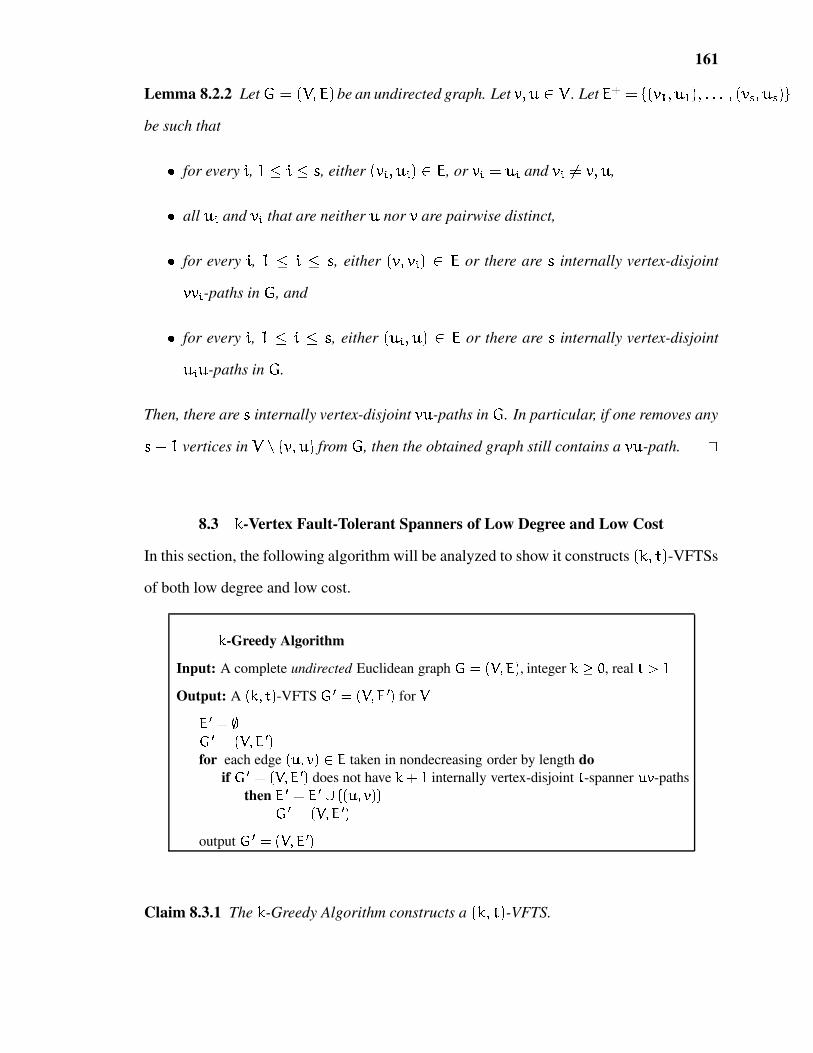
161

Lemma 8.2.2 Letû¾éP

be an undirected graph. Let « . Let å 8 ¯/ / P ''' ° N N ;

be such that

for every¦,3£«¦ ß , either

¥ -¥ , or ¥ -¥ and ¥ j ,

all -¥ and ¥ that are neither nor are pairwise distinct,

for every¦,3 ¦² ß , either

¥ or there are ß internally vertex-disjoint

à¥ -paths in

, and

for every¦,32w¦ ß , either

[¥ or there are ß internally vertex-disjoint

-¥ë -paths in

.

Then, there are ß internally vertex-disjoint º -paths in

. In particular, if one removes anyßéN 3 vertices intr 8ë [; from

, then the obtained graph still contains a º -path. ÕÖ

8.3 = -Vertex Fault-Tolerant Spanners of Low Degree and Low Cost

In this section, the following algorithm will be analyzed to show it constructs = -VFTSs

of both low degree and low cost.

c -Greedy Algorithm

Input: A complete undirected Euclidean graph 'zadY/|a e , integer c~ , real VE0hOutput: A adc|V e -VFTS ' zadY/|a e for Y z' z«adY|a e

for each edge a;|W e taken in nondecreasing order by length doif ' z«adY|a e does not have cóh internally vertex-disjoint V -spanner -paths

then z a;q|W eW' zadY|a eoutput ' z«adY|a e

Claim 8.3.1 The = -Greedy Algorithm constructs a = -VFTS.

162

Proof : Let be any subset of

having size at most = . First prove that

r£ is a

-spanner forr .

Pick any pair of points , inr´ . One has to show that

r[ has a -spanner

-path. Clearly, if , then this is true. So suppose that

. Then,

according to the algorithm, the only reason for not including edge in

is that there

are = x3 internally vertex-disjoint -spanner K -paths in

. Therefore, since = ,

there is at least one such path in r . á

Remark 8.3.2 Notice that Claim 8.3.1 holds even if the edges are taken in an arbitrary

order (that is, not necessarily nondecreasing).

Furthermore, this claim holds not only for Euclidean graphs and the assumption

that

is a complete graph can be weakened. For general graphs, a graph T T P T

is said to be a =JT T -VFTS of a weighted graph

§öéPif T E ,

Tµ , and for

any àµ

with =&T , for any pair of vertices ö 7r( , the graph T r)

contains a º -path of total length at most LT times the length of the shortest º -path intr7 . Then, the proof of Claim 8.3.1 implies that if one begins the = -Greedy Algorithm

with an arbitrary = xl3 -connected weighted graph

»ö, then the obtained graph will be a

= -VFTS of

.

8.3.1 Analyzing the Maximum Degree

This section is devoted to prove that the = -VFTS constructed by the = -Greedy Algo-

rithm has maximum degreeý² = . The analysis is in a similar spirit as the analysis of the

greedy algorithm for normal spanners, see, e.g., [1, 15].

Following is an auxiliary claim that will be used in later analysis.

Claim 8.3.3 Let 9¹Ï«Ï and suppose that is chosen such that 5 /cos 0 sin . Let ¾ . Let , , Ê be any three points in

with

P° Ê and ºÊ [ .

Suppose further that KW -ÊÅ . Then, for each -spanner Ê -path · in the path

consisting of the edge followed by the path · is a -spanner Ê -path.

163

Proof : Let · be any -spanner Ê -path in . Let be the -Ê -path obtained by taking

the edge followed by · . Then

length 2 KÅ x length

· KW x è ÊÅ' (8.1)

Furthermore, if denotes the point on the segment -Ê such that K LÊ A K° ,

then

ÊÅ x LÊÅ ÊW x§ N» q ' (8.2)

Next, observe that KÅ è sin K [ KÅ è sin and q KW è cos

5 KÅ è cos . Therefore, combining these two identities with (8.1) and (8.2), one obtains

length Ä KW x è ÊÅ KW x è -ÊÅ x W è sin (N cos

è -ÊÅ x KÅ è<3 N0 cos £N sin 'Hence, by the assumption that 5 3 cos ²N sin , one can conclude the claim that

length [ è -ÊÅ . áThis claim can be used to prove the following result.

Claim 8.3.4 Let 9bÏßÏ and t5 /cos 0 sin . Let

ÜP be the output of the = -

Greedy Algorithm for

. For any l , let be any cone in M with the apex at and

the angular diameter1 at most . Then, has at most = x3 edges incident to that are

contained in the cone .

Proof : Let be the set of edges in

incident to that are contained in the cone .

Let be the longest edge in

. The proof is to show that if there are more than =edges in

that are shorter than , then there are = xD3 -spanner K -paths in

, each

using only edges shorter than W . This will imply that the = -Greedy Algorithm would not

add edge to

, which contradicts to the fact that is an edge of

.Suppose there are = xÐ3

edges in that are shorter than

. Then one can

prove the existence of = xE3 internally vertex-disjoint K -paths such that each path uses

1The angular diameter of a cone in having its apex at point is defined as the maximumangle between any two vectors and ! , |W! .

164

edges in that are shorter than

. Consider first any edge such that . By Claim 8.3.3, the K -path consisting of the edges P° is of length

upper bounded by è KW .Next, consider any edge

such that . Then, since the = -

Greedy Algorithm has not taken edge to

, there must exist = x3 internally vertex-

disjoint -spanner -paths, and each edge on these paths is shorter than , which is

less than . Therefore, by Claim 8.3.3, there exist = x3 -spanner -paths between

and such that all paths begin with edge and then are internally vertex-disjoint.

Summarizing, there are = x3 vertices / 1 ''' æ' å / such that for each¦,3(«¦

= x3 , (i) ¥ and (ii) either

L¥ and q¥~ x L¥dW è KW , or contains

= xí3 -spanner K -paths between and such that all paths begin with edge ±¥

and then are internally vertex-disjoint, and each edge on each path is shorter than .

Therefore, one can apply Lemma 8.2.1 to conclude that contains at least = xÇ3 internally

vertex-disjoint -spanner K -paths, each path using only edges shorter than . This,

however, contradicts to the fact that is an edge of

, and hence, this completes the

proof of the claim. áIn [120], it was shown that there is a constant Ugv9 such that for any point ·2M$

and any angle , 9bÏÇÏ , there is always a collection ofb U± 0 / cones in M

having the apex at point · such that (i) E Ô + M , and (ii) each cone +Ð has the

angular diameter at most . One can incorporate this upper bound for the number of cones

in with Claims 8.3.1 and 8.3.4 to obtain the following lemma.

Lemma 8.3.5 Let

be any point set in a Euclidean space M . Let = be any non-negative

integer and let be any real number, v 3. Then, the = -Greedy Algorithm returns a = -VFTS for

having maximum degree of

D Uà 0 / = , where cos £N sin 5 /· . In

particular, if the dimension

and are constant, then the maximum degree isý² = . ÕÖ

165

8.3.2 Upper Bound for the Cost of Spanners Generated by the = -Greedy Algorithm

The most difficult and challenging part of the proof of Theorem 8.1.3 is the analysis of the

total cost of the spanner generated by the = -Greedy Algorithm. In order to bound the cost

of that spanner, one needs to first introduce the concept of “leapfrog property” [29], which

yields a bound for the total cost of a set of edges in terms of the relative position of these

edges in Euclidean space.

Definition 8.3.6 (Leapfrog property [29]) Let C5 3. Let

6 be a Euclidean

graph. A set T µ

satisfies the -leapfrog property if, for every ßz5E , for every subset å 8 ·[/ ¯/ P ''' ° · N N ;8µ T it holds that

è ·[/H¯/$Ï Nê¥Ìà1 ·W¥F¥~ x èO N ·[/ x N 0 /ê

¥Ì&/ ¥B·Å¥ å / 'The following result is shown in [29, 31] (see also [30, Theorem 3]).

Claim 8.3.7 Let be a constant greater than3. Let

6 be a Euclidean graph.

If a set Tµ

satisfies the -leapfrog property then the total cost of the edges in T

isb:¡ X¢¡ G , where

¡ X¢¡ G is the cost of an MST connecting the endpoints of T . The

constant implicit in the

-notation depends on and

. ÕÖThe following result gives a tight upper bound for the cost of

= -VFTSs gener-

ated by the = -Greedy Algorithm. This is one of the main results of this chapter; together

with Lemma 8.3.5, it directly yields Theorem 8.1.3.

Lemma 8.3.8 Letû¾

be a = -VFTS of a point set

generated by the = -Greedy

Algorithm. Then, the cost of

is at mostD = 1 è = MST

. The constant implicit in the

-

notation depends on and

.

Proof : The idea of the proof is to partition the edges of

intob = 1 groups and then

show that the cost of edges in each group is upper bounded byD = MST

.

First partition

into disjoint sets / P 1 ''' such that each

¥ is a maximal set

of edges and any two edges in the set have an angle at most where satisfies »5

1663 cos ¿N sin . By the discussion before (see also [120]), there areD Uà 0 / such

disjoint sets / P 1 ''' .

Next, partition each ¥ into sets

¥Õ/ P ¥®1 ''' such that each ¥Â, satisfies the -

leapfrog property. For each edge S ¾ , let 8µ be a minimum vertex set such

that after removal of all vertices of from

, there will be no -spanner º -paths con-

sisting only of edges shorter than S . Since

is a = -VFTS generated by the = -Greedy

Algorithm, besides S itself, there are at most = internally vertex-disjoint -spanner º -paths

having all edges shorter than S . Therefore, by Menger’s theorem one gets = .

Fix a set ¥ . Let

X be a subset of ¥ containing edges that are shorter than S and

that are incident to a vertex in . Then, define the sets

¥Õ/ P ¥®1 ''' by picking the edges

S) ¥ one by one and adding S to any set ¥d, that does not contain any edge in

X . One can

claim thatD = 1 sets

¥Â, are sufficient in the construction and that each set ¥Â, satisfies the

-leapfrog property. Indeed, by Claim 8.3.4, each vertex is incident to at most = x3 edges

in ¥ . Therefore, since = , it must be true that X = = x»3 . Thus, = = xl3Jx»3

sets ¥d, are sufficient for each

¦.

Fix a set ¥Â, . Now prove that

¥Â, satisfies the -leapfrog property. Let

8 P° PLP° / ¯/ P ''' & µ µ ; be any subset of ¥Â, . The goal is to show that

è P P Ï µê N / N N x è µ P x µ 0 /ê N P N N å / 'Observe first that this inequality is trivial if either P P µ P or P P

N N å / for certain ß , 9 ß .wN 3 . Furthermore, it is enough to consider the case when P° PL is the longest edge in . Therefore, from now on, it will be assumed that

P° PLis the longest edge in

È¢ 8ë P° /i; 8ë¯/ -1P; ''' 8ë µ 0 / µ ; 8 µ P ;£ .

For convenience, let S P^ P^ . Let be the graph obtained from

after

removing all vertices in together with their incident edges and then by removing all

edges not shorter than P° P^ . By the discussion above and by Menger’s theorem, any

P P -path in must have total length greater than è P P . The goal is to show that

167

* µ N &/ N N x è& µ P x * µ 0 /N P N N å / is at least the length of certain P P -path in .For each 8ËÊ TÍ; in

¢ 8 P° H/r; 8ë¯/ -1; ''' 8ë µ 0 / µ ; 8ë µ P ; £ , either Ê T

or there are = x²3 internally vertex-disjoint -spanner ÊÙT -paths in

consisting only of edges

shorter than Ê T , which is shorter than

P^ P^ by assumption. Furthermore, none of the

points P° / ''' µ P° ¯/ ''' µ is in . (Indeed, if, for example, N , then by

the assumption no edge incident to N should be included in ¥Â, , but this contradicts to the

fact that N N ¥Â, .)

Therefore, by Menger’s theorem there must be a -spanner ÊÙT -path in . Hence,

one can create a P P -path in as follows: starts with a -spanner P / -path, then

uses edge Ø/ ¯/ , then uses a -spanner Å/i-1 -path, then uses edge

´1 º1 , ''' , then

uses edge µ µ , and finally terminates with a -spanner µ P -path. By the discussion

above, is a P P -path in . Moreover, one can derive that

length Ä è P / x /B¯/ x è ¯/r-1° x -1î1° xÀèèè µ µ x è µ P

µê N / N N x è µ P x µ 0 /ê N P N N å / 'However, by the arguments above,

contains no -spanner P P -path. Therefore,

è P P Ï length ß µê N &/ N N x è µ P x µ 0 /ê N P N N å / ß

which implies the -leapfrog property of set ¥Â, .

To summarize the discussion, one can partition the set of edges of

intoD Uà 0 / è

= 1 sets of edges, each set satisfying the -leapfrog property. Therefore, by Lemma 8.3.7,

this concludes the proof. á

8.4 Efficient Construction of Fault Tolerant Spanners

In the previous section, it has been proved that the = -Greedy Algorithm generates = -

VFTSs with low maximum degree and low total cost. The disadvantage of this algorithm,

however, is that it is not known how to implement it efficiently. In this section an alternative

168

approach to construct fault tolerant spanners will be discussed. For convenience, in this

section directed graphs and their spanners will be considered.

First the notion of gap property and near parallel edges is introduced, and then a

new sufficient property for graphs to be = -VFTSs is prented. Then, one can use this

characterization to design a simple algorithm that generates good = -VFTSs in polyno-

mial time. Finally, algorithm is tuned to decrease the running time toD = log x

t= 1 log = .

8.4.1 Basic Auxiliary Properties

The following are two important notions on directed edges that will be heavily used in the

chapter.

Definition 8.4.1 (Near parallel edges) Two directed edges · and

Ê T are called n -

near parallel2 if after translating vector ¤ ¥Ê4T such that Ê coincides with · , that is, to the

vector ¤ ¥·R with TN ÊØN2· , the angle between vectors ¤ ¥·¦ and ¤ ¥·P is upper bounded by

n .

Definition 8.4.2 (Gap property) Let ¦Þ5À9 . Letû¾

be a directed Euclidean graph.

A set of edges TNµ satisfies ¦ -gap property if for any two edges

/ H/ P° 1 -1 Tthe distance between the heads and the tails of

W/ / and 1 -1 is greater than ¦ times

the length of the shorter of the two edges, that is,

min8 ¯/Õ1° /i-1° ;v ¦ èmin8P ¯/iH/ 11° ;D'

The following result is shown in [15]. (The constant implicit in the

-notation does

not depend on

.)

Claim 8.4.3 [15] (see also [6, Lemma 1]) Let ¦ v 9 . Letì

be a directed

Euclidean graph. If a set T µ

satisfies the ¦ -gap property then the total cost of the

2pairs of § -near parallel edges are called “similar directional” in [15].

169

edges in T is

D /¨ è log T èà¡ X¢©¡ G , where¡ X¢©¡ G is the cost of an MST connecting the

endpoints of the edges in T . ÕÖ

Our next claim states, informally, that if two edges in a directed Euclidean graph

are near parallel and close to each other, then one can form a spanner path between the

endpoints of the “longer” edge by concatenating the “shorter” edge and the spanner paths

between endpoints of the two edges. This claim is essentially proven in [6, Lemma 2].

Claim 8.4.4 Let , n , ¦ be real numbers such that 92Ï nÀÏLK^Î , 9 ¦ /1 cos nDNsin nÇN /· . Let

be a directed Euclidean graph. Let

and Ê be two edges in

that are n -near parallel to each other. Suppose KW Ê cos n , and ÊW . If

-ÊÅ ¦ è W , then (i) Ï4 Ê and (ii) è Ê" x KÅ x è è Ê . ÕÖRemark 8.4.5 It should be emphasized that Claim 8.4.4 holds not only when the length

of edge is less than or equal to the length of edge

Ê , but it also holds when

ÊLÏE KW Ê cos n .

Furthermore, notice that Claim 8.4.4 still holds if one changes the assumption

-ÊÅ ¦ è KÅ to -ÊW ¦ èmin8 KÅ Ê ; since the latter assumption is stronger. There-

fore, this claim is true when edges and

Ê do not satisfy the ¦ -gap property.

These two observations are important for the efficient algorithm described in Sec-

tion 8.4.3.

8.4.2 Sufficient Conditions for Being a = -Vertex Fault-Tolerant Spanner

In this section a new sufficient condition for a Euclidean graph to be a = -VFTS will

be presented. Later it will be shown how this condition can be used to obtain an efficient

algorithm for constructing = -VFTSs. The approach is motivated by a similar charac-

terization of spanners developed by Arya and Smid in [6].

170

Lemma 8.4.6 Let , n , ¦ be real numbers such that 9¿ÏEn2ÏK^Î and 9 ¦ /1 cos néNsin nHN /· . Let

ûéPbe a directed Euclidean graph. Suppose that for any two vertices

and in

,

1. either or

2. there are = x»3 edges 8 Ø/ ¯/ P ''' ° O' å / Ú' å / ;8µ such that

– for each3)«¦6 = xÀ3 , [¥Â¥ KW cos n ,

– all -¥ and ¥ that are neither nor are pairwise distinct,

– for each3)«¦6 = xÀ3 , edge

[¥ ¥ is n -near parallel to , and

– for each3)«¦6 = xÀ3 , min8P A[¥~ º¥Â ; ¦ è -¥d¥~ .

Then

is a = -VFTS for

.

Notice that in Lemma 8.4.6, it is allowed that some of the é¥ and ¥ are equal to or , but otherwise, all other endpoints of the edges in 8 $/ / P ''' ° 8' å / ' å / ; must be

pairwise distinct.

Proof : In order to prove that

is a = -VFTS, one need to show that for any two

vertices 2 , either or

contains = xl3 disjoint -spanner K -paths, each

-path having all edges shorter than KW cos n . The proof is by induction on the rank of

the distances between the pairs of points in

.

If has the minimum distance among all pairs of vertices, then must be an

edge of

, and hence the claim holds for . Next, one can proceed by induction. Consider

a pair of vertices Ù . By induction, for all ordered pairs of vertices Ê Tú with

ÊÙTHÏ4 KÅ , either Ê T or

contains = x3 disjoint -spanner ÊÙT -paths, each having

all edges shorter than ÊÙTH cos n . The goal is to prove that either or

contains

= x3 disjoint -spanner K -paths in

, each having all edges shorter than K cos n .

One only has to consider the case when . Then, by the lemma’s assump-

tion, there exist = x3 edges Ø/ / P° -1 1 P ''' ° O' å / Ú' å / in

such that

171

(i) for each3)«¦ = x»3 , edge

-¥ ¥ is shorter than KW cos n ,

(ii) all -¥ and ¥ that are neither nor are pairwise distinct,

(iii) for each3)«¦ = x»3 , edges

[¥ ¥ and are n -near parallel, and

(iv) for each3)«¦ = x»3 , min8 -¥~ ¥dW ; ¦ è -¥Â¥~ .

Pick any edge [¥ ¥ . Assume without loss of generality that ´¥~ min8 -¥~ ¥dW ; .

Since, [¥ ¥ and

are n -near parallel by (iii), [¥Â¥~ KW cos n by (i), and

¥~ ¦ è ¥Â¥~ by (iv), Claim 8.4.4 (i) implies that ¥dW[Ï KW . Hence, by induc-

tion, either ¥ or there are = xl3 disjoint -spanner ¥Â -paths in

, all using only

edges shorter than ¥ÌÅ cos n . Similarly, since A[¥~ º¥ÌÅ±Ï¾ K , either [¥ or

contains = xß3 disjoint -spanner [¥ -paths that use only edges shorter than ´¥~ cos n .

Furthermore, by Claim 8.4.4 (ii), each K -path consisting of a -spanner é¥ -path (or edge -¥ ), edge -¥ ¥ , and a -spanner ¥Â -path (or edge

¥ ) is a -spanner -path.

So far it has been proven that there are = x¿3 edges / ¯/ P° 1 1 P ''' ° O' å / Ú' å /

such that for each¦,3Ä¦ = x¾3

, (i) either ´¥

or

contains = xw3dis-

joint -spanner A[¥ -paths that use only edges shorter than ´¥~ cos n , and (ii) either ¥ or there are = x3 disjoint -spanner ¥d -paths in

that use only edges short-

er than ±¥ cos n . Now, the claim follows directly from the Menger’s theorem (for more

details, see Lemma 8.2.2). áEssentially identical arguments can be used to prove the following characterization

for edge fault-tolerant spanners.

Lemma 8.4.7 Let , n , ¦ be real numbers such that 9²ÏínÏ Í^Î , 9 ¦ /1 cos nyNsin ntN /· . Let

û6 be a Euclidean graph. Suppose that for any two vertices and

of

, either or there are = x§3 edges 8 Ø/ ¯/ P ''' ° O' å / Ú' å / ;Nµ

such

that

for3(¦H = x3 , -¥Â¥ KÅ cos n ,

172

each edge [¥ º¥ is n -near parallel to

, and

for each3(«¦ = x»3 , min8 -¥ ¥ÂÅ ; ¦ è -¥Â¥~ .

Then

is a = -EFTS for

. ÕÖ

c -Gap-Greedy Algorithm

Input: A directed complete Euclidean graph 'zadY/|a e , § and ª , and integer c such thatc~ , ¬«§®«¯|Ä±° , and e«tª²« /1 a cos §³ sin § eOutput: A adc|V e -VFTS ' zadY/|a e for Y , where Vqzh¤Äa cos §³ sin §³yñ´ª e .

zfor each edge a;q|W e taken in nondecreasing order by length do

Let T be a maximal (in the sense of inclusion) subset of such that:

1. all edges in beginning at or ending at are contained in T ,2. for every aµ |W! e T , aµ |W! e is § -near parallel to a;|W e ,3. for every aµ |W! e T , min

^ ©^¶|^ !©^ ïª óT^ ·!/^ ,4. for any pair of distinct edges aµ ©|W! e |a¸.9|W¹ e T , if ºz and !²ºzs , then »ºz. and !sºz¼¹ .

if ^ T ^½«cóh then z ¾ a;q|W eWoutput ' zadY|a e

Figure 8.2 The = -Gap-Greedy Algorithm

The characterization of = -VFTSs in Lemma 8.4.6 almost immediately implies

a simple polynomial-time algorithm for constructing such spanners, which is called = -Gap-

Greedy Algorithm and describe in a form of a meta-algorithm in Figure 8.2.

The following central lemma describes main properties of the = -Gap-Greedy Algo-

rithm.

Lemma 8.4.8 The = -Gap-Greedy Algorithm outputs a directed = -VFTS for E3 cos nÍN

sin ntN¹¬¦ with maximum in-degree and out-degreeb = and whose total cost is

D /¨ è= 1 log times the cost of an MST for

. The constant implicit in the

-notation depends

on and

.

173

Proof : First it will be prove that is a

= -VFTS by showing that for any ordered

pair of vertices , one of the two conditions of Lemma 8.4.6 is satisfied. If ,

then the first condition is obviously true. Otherwise, and consider the iteration

of the algorithm when is chosen. The only reason that

is not added to is

that T±5û= xÙ3 . But this implies that the second condition of Lemma 8.4.6 is satisfied for . Therefore, is a

= -VFTS by Lemma 8.4.6.

Next, it will be prove that the maximum out-degree and the maximum in-degree of

each vertex isD = . Let be any vertex. First prove the out-degree of is

b = . Let

+Í be any cone in M with the apex at and the angular diameter at most n . Let E be

the set of edges in beginning at that are contained in the cone +- . It will be proved

that E = x 3, which immediately implies that the out-degree of is

b = . Now

analyze the behavior of the algorithm at the moment when E = x¹3 and the algorithm

considers a new edge with y0+ . Observe that in that case one will have

E µ T ,and hence,

T will be of size at least = xl3 . Therefore, the algorithm will not add the edge to the spanner. This implies that E = xE3 , and hence, the out-degree of isb = . One can use essentially identical arguments to prove the in-degree of isD = .

(Similar arguments show that is the head/tail of at most = xE3 pairwise n -near parallel

edges.)

Finally, one needs to prove that has small cost. One can proceed similarly as in

the proof of Lemma 8.3.8 and first partition into disjoint sets

/ P 1 ''' such that each ¥ is a maximal set of edges which are n -near parallel. By the discussion in the proof of

Lemma 8.3.8, there areb Uà°n 0 / such disjoint sets

/ P 1 ''' . Let us fix one set ¥

and divide the edges in ¥ into a minimal number of groups such that the edges in the same

group satisfy the ¦ -gap property. It will be proved thatb = 1 groups are sufficient. It is

enough to show that for any edge SÇ ¥ there are at mostD = 1 edges SÚ ¥ shorter

than S such that 8S SÚ ; does not satisfy the ¦ -gap property.

174

Fix an edge ¥ . Let

ã æ 8Õ·E ¿Í · ¥ ·¦W KW 9 ·´ ¦ è ·àW ; and let

ã æ be the set of edges in ¥ that (i) begin at vertices in

ã æ ,and (ii) are shorter than W . Note that since

ã æ µ ¥ , all edges in ã æ are pairwise

n -near parallel. One can show that ã æ ÅÏ = xE3 1 by contradiction. Suppose that

ã æ W5¾ = xú3 1 and consider the iteration in which the edge is picked by the

algorithm. Let T be the set taken by the = -Gap-Greedy Algorithm when the edge

is considered. It will be proved that T -5 = xÐ3

, which contradicts to the assumption

that . Let À be the set of all edges in

shorter than such that for every

edge SÙÀ , (i) S is n -near parallel to and (ii) 8 S ° ; does not satisfy the ¦ -

gap property. Note that because the algorithm picks edges in nondecreasing order, the

condition 3 of the algorithm implies that none of the edges in T satisfies ¦ -gap property

with . Thus,

T can be defined as the sum of certain maximal matching in À and the

set of all edges in À that either begin at or end at . Therefore, to prove that T ^5À= xÀ3it is sufficient to show that every maximal matching in À contains at least = x 3

edges.

Furthermore, because of the well known relation between the cardinality of the maximum

matching and the minimum cardinality of a maximal matching, it is enough to show that the

maximum matching in À contains at least = x»3 edges. One can prove this property by

considering the edges in ã æ . First observe that by the definition

ã æ µÀ . Therefore,

one only must show that ã æ has a matching of size at least = xE3 . Note that there

are at most = xl3 edges in ¥ starting at each vertex as proved above. Since it is assumed

that ã æ J54 = x§3 1 , one can conclude that set ã æ must contain at least = xú3

disjoint edges. Therefore, there is a matching of size at least = x»3 in À . But this leads

to a contradiction, and hence one proved that ã æ Ï = x3 1 .Symmetrically, one can define

ã æ , and prove that ã æ Ïû = x3 1 . Therefore,

ã æ È ã æ Ï4Î = xE3 1 . Hence one can conclude that one needs at most Î = x§3 1groups of edges from

¥ such that the edges in each group satisfy ¦ -gap property. Thus,

it is proved that one can partition the edges in into

b Uà±n 0 / = 1 groups such that the

175

edges in each group satisfy ¦ -gap property. To conclude the proof one can apply Claim

8.4.3 to obtain an upper bound for the total cost of to be

D Uà±n 0 / = 1 /¨ log times

the cost of minimum spanning tree of

. á

8.4.3 Efficient Construction of = Fault-Tolerant Spanner

It is easy to implement the = -Gap-Greedy Algorithm in polynomial time, however, direct

implementations lead to the running time ofw 1 . This section discusses how that algo-

rithm can be modified to achieve the running time ofb t= log x t= 1 log = while still

returning a spanner having the parameters promised in Lemma 8.4.8. The new approach

is similar to the one developed by Arya and Smid [6] to construct spanners with bounded

degree and low cost.

The main idea behind the new approach is not to consider all theý² 1 edges but

to have an efficient procedure that will “forbid” certain edges without considering them

explicitly during the run of the algorithm. Since every vertex is of degreeb = , the goal

is to ensure that onlyb = edges incident to any vertex are considered by the algorithm.

The rules of inserting an edge in the = -Gap-Greedy Algorithm will be relaxed in order to

obtain a more efficient implementation. On one hand, the goal is to maintain the properties

of the output spanner required by Lemma 8.4.6 and on the other hand, the aim is to output

a spanner having properties described in Lemma 8.4.8. Below the main idea is described

behind that relaxation, and the algorithm itself is described in Section 8.4.3.

Main idea behind the modified algorithm A collection of cones of angular diameter n(see, Section 8.3.1) will be used to test whether two edges are n -near parallel to each other.

That is, it is assume that there is a collection of cones with apexes at the origin and the

angular diameter n , so that the cones in cover MØ . Then, an edge is said to be in

a cone + if the vector ÑN4l+ . Using this notion, each time a pair of points with §+ are consider, one only needs to look at those edges Ê T that are in + .

176

Since if and

Ê T are in the same cone, then they are n -near parallel to each other,

this notion allows one to relax testing of n -near parallel edges.

Once the collection of cones is fixed, the cones from will be considered sepa-

rately. The spanner is built by defining the edge set which will be the union of the edge

sets constructed for each cone separately. Let E denote all those edges of

inside the

cone +«f .

In the = -Gap-Greedy Algorithm, one analyzes the edges in the order of their in-

creasing lengths. This is more complicated (in the sense of efficiency) if one wants to

consider the edges being in different cones separately. Therefore, following the approach

from [103] (see also [6]), one can approximate the distance between the points in a cone.

For each cone + , fix a ray Ø E that is incident to the apex of + and that is included in the

cone + . Then, the idea of approximating the distance between pairs of points is to use the

distance between the projections of the points on the ray Ø E . To make this notion more for-

mal, a few definitions are needed. For any cone +«¼ and any point ÊyDM , let + Ò be the

translation of + so that the apex of + Ò is at Ê , that is, + Ò 8T02M6 TtNÊy0+; . Similar-

ly, for the ray Ø E , let Ø E Ò 8TÙDMH T¿NÊb Ø E ; . Then, one can approximate the distance

between the points in the cone + using the following function dist E :

dist E Ê T K 9:; :< Ê U if TÙ0+ Ò and U is the orthogonal projection of T onto Ø E Òn

if T»0+ Ò 'The main reason of using this approximation of the distances between pairs of points inside

a cone is that it can be efficiently maintained by a dynamic algorithm (see also [6, 103]).

Furthermore, it is easy to show that if dist E Ê T © dist E , then ÊÙT6 KW cos n .

Therefore, by Claim 8.4.4 and Lemma 8.4.6, the algorithm remains correct (in the sense

that it satisfies the properties from Lemma 8.4.6) even if edge Ê T is considered before

edge .

Summarizing, the algorithm is going to consider the edges inside each cone in non-

decreasing order of their dist E length.

177

Let Ê T be an edge in a cone +C¼ that is to be taken by the algorithm. Observe

that if there are already at least = x3 edges in + with the head at Ê then the edge Ê T will

not be taken by the algorithm. Therefore, whenever a vertex Ê already has = xl3 outgoing

edges in + , then no further edge starting at Ê in + will be considered. Symmetrically, one

only needs to consider at most = x3 incoming edges for any point T .

The other reason for rejecting edge Ê T is that there are many disjoint edges in

+ which are shorter than Ê T with respect to dist E length and are very close to either Ê

or T . Let ÊÙ be any input point. Two special data structures will be used to maintain

a maximal set of disjoint edges in + that have starting or ending points close to Ê , respec-

tively. These two data structures will be modified not when an edge in + incident to Ê is

considered, but instead, they will be updated each time an edge close to Ê is inserted in-

to E . To be more precise, at each moment of the algorithm, a set Á E Ê is maintained for

each Ê which contains a set of disjoint edges in E such that for any

0Á E Ê , Ê" ¦ è W . Similarly, R E Ê is maintained to contain a set of disjoint edges in

E such

that for any R E Ê , ÊÅ ¦ è KW .

Now, suppose an edge is inserted to

E . Letk ã æ and

k ã æ be the set of

points that are at distance at most ¦ è KÅ from and , respectively. By the definitions of

Á E Ê and R E Ê , one needs to update those points ink ã æ and

k ã æ that are “affected”

by the edge . That is, for every point Ê k ã æ , if Á E Ê contains no edge incident

to either or , then one updates Á E Ê by inserting to it. Similarly, one updates

R E T for every point T k ã æ .Notice that the operation of updating the sets Á E Ê and R E Ê may be very expen-

sive, because both the vertex setsk ã æ , k ã æ and the edge sets Á E Ê , R E Ê may be very

large. Therefore, one can relax the definition of the sets Á E Ê and R E Ê by observing that

once Á E Ê or R E Ê is of size larger than or equal to = xC3 , by Lemma 8.4.6, no new edge

in + beginning or ending at Ê , respectively, will have to be added to E . Therefore, two sets

of points from

are maintained: /E containing all points that still can be the heads of new

178

edges in E and

1E containing points that still can be the tails of new edges in E . Each

time the size of certain Á E Ê is greater than or equal to = x¹3 , Ê is deleted from /E ; no fur-

ther edges in + that begin at Ê will be considered, Á E Ê will not be updated anymore, nor

will Ê be considered in any further setsk ã æ . Similarly, if R E Ê 5 = x§3 , Ê is deleted

from 1E , no further edges in + ending at Ê will be considered, R E Ê will not be updated

and Ê will not be considered in any further setsk ã æ . In this way, since both Á E Ê and

R E Ê have a size between 9 and = x3 , the total number of operations for updating the sets

Á E Ê and R E Ê in the entire algorithm (for a given cone + ) will beb =6 .

Observe that once a vertex Ê has been reported = x3 1 times in the setsk ã æ ,

then there are = xú3 1 edges such that -ÊÅ ¦ è KW . Since each vertex is the

head of at most = x§3 edges in + , there must be = x§3 disjoint edges among all these

edges. Therefore, in this case, the size of Á E Ê must be greater than or equal to = xû3 (see

Lemma 8.4.8 for a more detailed discussion on similar arguments). Hence, at this moment

Ê will be deleted and will not be reported ink ã æ for any any more. For the same

reason Ê will be reported ink ã æ at most = x3 1 times. This allows one to conclude

that the total size ofk ã æ and

k ã æ for all vertices and in the entire algorithm (for a

given cone + ) is Î´ = x»3 1 .To define sets

k ã æ one needs to find all points that are at the distance at most

¦ è KW from . However, since it is difficult to maintain dynamic data structures to findk ã æ in the Euclidean metric, in the definition ofk ã æ one assumes the distances between

points according to the ÝLÁ metric. That is,k ã æ is redefined to be the set of all points

Ê with -ÊÅ Á ¨I KW . (Here, one needs to output only the points that have not been

deleted, that is, those Ê for which Á E Ê &Ïw= xE3 .) Since -ÊÅ Á ¨I KÅ implies that

-ÊÅ ¦ è W , the new definition ofk ã æ gives a subset of the set

k ã æ defined above.

Setk ã æ is redefined symmetrically.

179

Improved = -Gap-Greedy Algorithm In the previous subsection the main ideas behind

the modifications of the = -Gap-Greedy Algorithm are presented. These ideas allow one to

design a new algorithm that finds good fault-tolerant spanners efficiently. A more formal

description of the algorithm is presented below, on page 184. A formal proof of its cor-

rectness will be given first and then an efficient implementation of the algorithm will be

discussed.

Properties of the Improved = -Gap-Greedy Algorithm. This section is devoted to a

formal proof of the following lemma.

Lemma 8.4.9 Let

be a set of points in MØ . Let n , ¦ be real numbers such that 9)ÏEnÇÏK^Î and 9¿Ï¦wÏ /1 cos n²N sin n . Let Ð3 cos n²N sin n²N¹e¦ . There is a constant

U such that the Improved = -Gap-Greedy Algorithm outputs a directed = -VFTS with

maximum in-degree and out-degreeb = and whose total cost is

D Uà±n 0 / I ¨ = 1 log times the cost of a MST for

.

Proof : One needs to prove that the output of Improved = -Gap-Greedy Algorithm has

the same properties as the output of = -Gap-Greedy Algorithm after some conditions are

relaxed. The proof is similar to that of Lemma 8.4.8.

Let be the output of the Improved = -Gap-Greedy Algorithm. First,

is proved

to be a = -VFTS by showing that

satisfy the conditions of Lemma 8.4.6. Let be any ordered pair of vertices, and gNÙEÀ+ for some +ús . If

E , then the

first condition is obviously true. Otherwise, E and there are two possible reasons

why was not inserted to

E .

i. is considered explicitly in the “while” loop but is not inserted to

E .

In this case, dist E is minimum at the beginning of certain iteration. Since

is not added to E , there must exist either = x03 edges with heads at or = x03 edges

with tails at which are already inserted to E . These edges have length at most

180

W cos n , are n -near parallel to , and they have one common endpoint with . Therefore, the second condition of Lemma 8.4.6 is satisfied.

ii. is deleted when some other pair

Ê T is picked and added to E in the “while”

loop.

In this case, the only reason that is deleted from

E is either Á E = xÇ3 or

R E = x3 after Ê T is inserted to Á E or R E respectively. Suppose that

Á E = xÀ3 and consider the edges in Á E K 8 Ê/ Té/ P ''' ° ÊÚ' å / TÅ' å / ; . By

the Improved = -Gap-Greedy Algorithm, edge Ê¥ TK¥ , 3(«¦H = x23 , can be inserted

to Á E only if: (a) -Ê¥ Á ¨I Ê¥TK¥~ , which implies that Ê¥ ¦ è Ê¥TK¥~ , and

(b) Ê¥ T¥ is disjoint with all other edges in Á E . Furthermore, since

Ê¥ TK¥ is considered before

by the algorithm, it must be true that d¦ ß E Ê¥ TK¥ y

d¦ ß E , which means Ê¥TK¥~ KW cos n . Therefore, one can combine with (a)

and (b), to see that the second condition of Lemma 8.4.6 is satisfied.

To summarize, it has been proved for each pair Ê T , either

Ê T is an edge in

or there are = x3 edges in satisfying the second condition of Lemma 8.4.6. Therefore, is a

= -VFTS.

Next, it will be proved that the maximum in-degree and out-degree of each vertex

isb = . The proof is basically the same as the proof of Lemma 8.4.8. Let be any vertex.

According to the Improved = -Gap-Greedy Algorithm it is easy to see at most = xl3 edges

beginning at can be added to the E for any given cone +«¼ . Therefore the out-degree

of in is

D = . Similarly, one can show that the in-degree isb = .

Finally, one needs to prove that has small cost. Fix a cone + and divide the

edges in E into a minimal number of groups such that the edges in the same group satisfy

the¨I -gap property. It will be proved that

b = 1 groups suffice. To prove this claim it

is enough to show that for any edge Sß E there are at mostb = 1 edges SÚ´ E that

181

are “shorter” than S in terms of the dist E length and such that 8S SÚ ; does not satisfy theÏ -gap property.

Fix an edge E . Let

ã æ 8 Ê T E dist E Ê T Ï dist E and

-ÊÅ Ï è Ê4T ; and ã æ 8 Ê T E dist E Ê T Ï dist E and ÙT6 Ï è ÊÙT6 ; .

Observe that if an edge Ê T is “shorter” than

with respect to the dist E length and it

fails to satisfy theÏ -gap property with

, then Ê T ã æ È2 ã æ . Therefore, to

prove the claim it is sufficient to show that ã æ È2 ã æ D = 1 .First it will be proved that ã æ §b = 1 . Let À ã æ 8 Ê T E dist E Ê T Ï

dist E and -ÊÅ Á Ï è ÊÙT6 ; . Note that since -ÊÅ Á -ÊW , ã æ µÀ ã æ . In the fol-

lowing it will be shown that À ã æ §b = 1 which directly implies that ã æ D = 1 .There are two observations. First because all edges in À ã æ are “shorter” than

with respect to dist E , all these edges are picked and inserted to

E by the algorithm before . Secondly, each time after one of these edges Ê T is inserted to

E , the algorithm

inserts Ê T to Á E if

Ê T is disjoint with edges already in Á E . In other words, at

the end of each iteration of the Improved = -Gap-Greedy Algorithm Á E keeps a maximal

matching of the edges in À ã æ that have been inserted to E so far.

Now one can prove by contradiction that À ã æ Ï = xÑ3 1 . Suppose that À ã æ ±5 = x23 1 . It has already been shown that each vertex has out-degree (in-degree) in E of at

most = x3 . Therefore, the maximum matching of À ã æ must contain at least = x3 edges

and thus any maximal matching of ã æ must have at least

= x¹3 edges. Since Á E is a

maximal matching of À ã æ , Á E °5û= xÇ3 . Then, there must exist an edge Ê T ÂÀ ã æ

such that during the iteration when Ê T is inserted to

E , Ê T is also inserted to Á E ,

and Á E becomes = x»3 . However, the Improved = -Gap-Greedy Algorithm is designed

such that in that moment must have been deleted from /E and all edges with head at

including are also deleted from

E and will not be inserted to E . This contradicts

to the fact that E . Thus, it is proved that ã æ À ã æ Ï = x3 1 .

182

In a similar way, one can prove that ã æ Ïû = xg3 1 . Therefore, ã æ Èé ã æ ÏÎ = xÀ3 1 . Hence, one can partition the edges from ¥ into at most Î = x3 1 groups such

that the edges in each group satisfy the¨I -gap property. Thus, the edges in

can be

partitioned intoD Uà±n 0 / = 1 groups such that the edges in each group satisfy

¨I -gap

property. To conclude the proof one can apply Claim 8.4.3 to obtain an upper bound for

the total cost of , which is

b U±±n 0 / = 1 I ¨ log times the cost of MST of

. á

Details of the implementation of the Improved = -Gap-Greedy Algorithm. The de-

scription of the Improved = -Gap-Greedy Algorithm is on a high level and now it will be

disscussed how one can implement that algorithm efficiently. In order to obtain an efficient

implementations one must provide efficient data structures that allow one to query for (i) an

edge E with minimum dist E , (ii) the number of edges in

E beginning or ending

at , (iii) reporting all points ink ã æ and

k ã æ , and (iv) for verifying if an edge is

disjoint to all edges in Á E Ê or R E Ê .It is easy to see that one can maintain the data structure (ii) reporting the number

of edges in E beginning or ending at a given vertex with constant query time and update

time. Similarly, one can easily maintain the data structure (iv) verifying if an edge

is disjoint to all edges in Á E Ê or R E Ê withD

log = query time and update time. (The

bound for the query time follows immediately from the fact that Á E Ê or R E Ê containsb = edges and one can use a balanced binary search tree to store the endpoints of these

edges.)

Arya and Smid [6] gave an efficient data structure supporting queries (i) for an edge

in E with minimum dist E . As it is demonstrated (and discussed in details) in [6], the total

running time needed to perform all these operations is in our caseb t= log . (This

bound follows from the fact that one can use query (i)D =6 times, and as shown in [6],

efficient data structure can be built in timeb log that has constant query time andb

log amortized update time per edge.)

183

To efficiently report all points ink ã æ and

k ã æ one can use dynamic data struc-

ture for orthogonal range queries (see [88]). The algorithm only deletes points and therefore

the amortized deletion time isb

log 0 / and the query time isD

log 0 / time plus the

number of reported points [88]. Since each point is deleted at most once, the total dele-

tion time isD log 0 / . A query operations is performed on the dynamic data structure

each time after an edge is inserted, so the total time isD = log 0 / for

D = edges.

Each vertex is reported at mostD = 1 times, when reported, one needs to verify whether

Á E Ê or R E Ê can be enhanced by adding an edge, the verification and update takes timeblog = , thus the total time for reporting, verification, and update is

b = 1 log = .In summary, one can conclude the discussion in this section with the following

lemma.

Lemma 8.4.10 Let

be a set of points in MØ . Let n , ¦ be real numbers such that

9)ÏEnßÏK^Î and 9Ï¦wÏ /1 cos nmN sin n . Let 43 cos nzN sin nmNe¦ . There is a

constant U such that the Improved = -Gap-Greedy Algorithm can be implemented to run in

timeb U±±n 0 / = log x = 1 log = . ÕÖ

One can conclude the discussion in this section with the following main theorem

that follows immediately from Lemmas 8.4.9 and 8.4.10.

Theorem 8.4.11 Let n , ¦ be real numbers such that 9zÏín¹Ï K^Î , 9²ÏÃ¦ Ï /1 cos nyNsin n . Let

be a set of points in M . Let 3 cos nN sin nNle¦ . There is

a constant U such that inb U±±n 0 / t= log x = 1 log = time the Improved = -

Gap-Greedy Algorithm computes a directed = -VFTS having the maximum degree ofb U±±n 0 / = and the total cost of

D Uà±n 0 / = 1 Ñ ¦ log u= MST

. ÕÖ

To conclude this section, notice that Theorem 8.4.11 implies directly Theorem 8.1.4.

184

Improved c -Gap-Greedy Algorithm

Input: Set Y of Ã points in , an integer c~ , and positive §P|Äª with §®«¯|Ä±° andªÅ« /1 a cos §³ sin § eOutput: A adc|V e -VFTS ' zadY/|a e for Y , where VqzCh¤Äa cos §³ sin §³ñ´ª e .let Æ be any collection of cones with angular diameter § that cover for each cone Æ do

E z a;q|W eLÇ dist E a;q|W e «sÈ É E contains all edges a;q|W e such that F³Ê /Ë E z É E collects the edges in E that are to be included in the spanner Ëfor each Y do Z E aµ e zÉ Z E aµ e contains disjoint edges in E that begin at points near to Ëfor each Y do E aµ e zÉ E aµ e contains disjoint edges in E that end at points near to ËY /E zY É Y /E contains all points in Y such that ^ Z E aµ e ^«cØóhqËY 1E zY É Y 1E contains all points in Y such that ^ E aµ e ^½«cóhËwhile E ºz do

let a;|W e E be such that dist E a;|W e is minimal

if the number of edges beginning at in E is at least c$óh then

delete from Y /E and delete from E all edges beginning at if the number of edges ending at in E is at least cóh then

delete from Y 1E and delete from E all edges ending at if a;q|W e is still in E then É edge a;|W e will be in the spanner Ë E z E¬Ì a;|W eW E z E a;|W eW

let ñ ã æ be the set of points Y /E with ^ O ©^ Á ï ¨I ^ ©^let ñ ã æ be the set of points ! Y 1E with ^ ·!/^ Á ï ¨I ^ ©^for each ñ ã æ do

if a;q|W e is disjoint with all edges in Z E aµ e thenZ E aµ e zZ E aµ e a;q|W eWif ^ Z E aµ e ^·~ÇcØóh then

delete from Y /E and delete from E all edges beginning at for each ! ñ ã æ do

if a;q|W e is disjoint with all edges in E aJ! e then E aJ! e z E aJ! e a;|W eWif ^ E aJ! e ^T~ßcØóh then

delete ! from Y 1E and delete from E all edges ending at ! zsÍ E Ô E output ' zadY/|a e

CHAPTER 9

CONCLUSIONS

This dissertation studied combinatorial optimizations problems arising from two areas:

scheduling and network design. The main focus was to design efficient approximation

algorithms for NP-hard problems.

9.1 Scheduling Problems

In the scheduling area, problems in master-slave model have been considered. The master-

slave model finds many applications in parallel computer scheduling and industrial settings

such as semiconductor testing, machine scheduling, transportation maintenance and paral-

lel computing.

The complexity issues are considered first. It is shown that many makespan and

total completion time problems with constraints such as canonical, order preserving and

no-wait-in, are NP-hard in the strong sense.

Motivated by the computational complexity, some special cases of the problem are

considered. Several efficient algorithms are designed to minimize the total completion time

and makespan. These algorithms are proven to have very good approximation ratio. Next

more general cases are discussed. A job can have an arbitrary release time and arbitrary

processing time. There can be a single master, multi-masters, or distinct preprocessor and

postprocessors. Constant approximation algorithms are designed for the total completion

time problem. It is shown that these algorithms give good approximation for makespan at

the same time.

There are several questions that have not been answered. In this dissertation, it is

assumed that there are no precedence constraints among the jobs. These assumption may

not hold in some applications. It is worthwhile to develop approximation algorithms which

185

186

work well even with precedence constraints. Only the makespan and total completion time

are considered so far. Other objectives such as maximum lateness, number of tardy jobs

and total tardiness, have not been studied. In view of the NP-hardness of makespan and

total completion time, minimizing these objectives must also be NP-hard. In that case, it

will be desirable to have good approximation algorithms.

9.2 Network Design Problems

The survivable network design problem is the problem of designing graphs that resist edge

and/or vertex removal. This is a fundamental problem in algorithmic graph theory with

numerous applications in computer science and operations research. It is well-known that

all non-trivial variants of the survivable network design problem are NP-hard and therefore

the main research interest lies in the design of efficient approximation algorithms.

First the geometric version of the survivable network design problem is considered.

A PTAS is developed for the 8:9 3" "; -connectivity problem in which each vertex has a

connectivity requirement at most . Then it is shown that the techniques can be generalized

to other Ø ~ metrics and to the 8<9 3" ''' =; -edge-connectivity problems for multigraphs.

PTASs or Quasi-PTASs are designed for the minimum -connectivity problem and some

of its variations in unweighted or weighted planar graphs.

Then the problem of efficient construction of fault-tolerant spanners are considered.

A greedy algorithm is presented which finds the fault-tolerant spanners with both maximum

degree and total cost asymptotically optimal. An efficient algorithm is then developed to

find a fault-tolerant spanners with asymptotically optimal bound for the maximum degree

and almost optimal bound for the total cost.

Two important components used in all the approximation schemes are hierarchical

decomposition and dynamic programming. Through the decomposition, a large graph is

decomposed into smaller ones which have small interface with the rest of the graph. In

the Euclidean space, random shifted dissection is used to decompose a set of points into

187

regions. The interface between two regions contains only constant number of portals. In

planar graphs, a modified separator theorem is developed and applied to decompose the

graphs into small pieces. Each small piece has at most logarithmic number of portals. The

small interface between subgraphs allows one to solve the problem by dynamic program-

ming in polynomial time.

It would be great if one can extend the above techniques to other related problems.

Following are some possible problems.

= -connectivity problem in doubling metrics. The doubling dimension of a metric is the

smallest = such that any ball of radius can be covered using ' balls of radius . This

concept for abstract metrics has been proposed as a natural analog to the dimension of a

Euclidean space. Doubling metric appears in several practical applications such as peer-to-

peer networks and data analysis. In [114], Talwar showed that for low dimensional metrics

there exist quasi-polynomial time approximation schemes for TSP and other optimization

problems.

The geometric version of the = -connectivity problem has been considered and poly-

nomial approximation schemes have been designed = -connectivity problem in geometric

graphs by Czumaj and Lingas in [26]. Their algorithm is based on the framework of Arora

[3]. Like the approach used by Rao and Smith [101] for the TSP problem, their algorithm

depends on spanners and some other nontrivial techniques.

For the problem in the low dimension doubling metric, there is no known results

about construction of light and sparse spanners. Therefore one can not use the approach as

in [26]. However, it is still possible to achieve a Quasi-PTAS by using some novel ideas

and those from [114], [27] [26].

Minimum strongly connected subgraph in planar graphs. For the general unweighted

graphs, constant approximation algorithms have been given by Khuller et al. in [71, 72].

188

The existing separator theorems only work for undirected graphs. A PTAS for the problem

in planar graphs will heavily depend on light, directed cycle separators.

Forbidden minor -ECSS (or -VCSS). There are two difficulties here: first, the usual

separator theorems do not produce cycles (just trees). Also the appropriate generalization

of Lemma 6.2.4 may require a careful application of the Robertson-Seymour theory, which

appears difficult. For the special case of bounded-genus graphs, both of these issues look

more tractable.

For the fault tolerant spanners, an obvious open question that is left is whether one

can design an efficient algorithm that outputs fault-tolerant spanners having properties from

Theorem 8.1.3. It is believed that it should be possible to design anD = polylog -time

algorithm for that problem.

In all existing analysis of fault-tolerant spanners, the cost of fault-tolerant spanners

is compared with that of MST. Since a = -fault-tolerant spanner must be = x3 connected, a

natural question is how to compare its cost with the cost of the minimum = x3 connected

spanning subgraphs. One can extend the example in Figure 9.1 to show that the cost ratio

between the optimal:3"3x u fault-tolerant spanner and the minimum

= xl3 connected

spanning subgraphs can be arbitrarily large in planar graphs. It is believed that the cost

ratio for the geometric graphs should be bounded by constant. It is desirable if one could

design efficient algorithm to construct such light spanners.

There are many algorithmic applications of spanners, perhaps the most appealing

being the recent application in anb log -time approximation algorithm for the Eu-

clidean TSP [101]. On the other hand, not many applications of fault-tolerant spanners are

known. Actually, even in the most natural application to the = -connectivity problem, the

fastest approximation algorithms do not use fault-tolerant spanners [25, 26, 27]. Therefore,

investigating the relationship between the connectivity problems in Euclidean graphs and

the notion of fault-tolerant spanners would be an interesting topic.

189

1

2

2

21

1 1

1

1

(c)(b)(a)

1

1

1

1 1

1 1

1

1

2

2

21

1 1

Figure 9.1 (a) A weighted planar graph ' , (b) the minimum cost biconnected spanning subgraphof ' , (c) the optimal aihT|hÍóÎ e fault-tolerant spanner which is ' itself.

ε/8 ε/8 ε/8 ε/8 ε/8ε/8 ε/8

(a)

(b) (c)

10

10−ε

10−ε 10−ε 10−ε

10−ε 10−ε

Figure 9.2 (a) A weighted planar graph ' , (b) aihT|hóCÎ e -VFTS (or aihT|hóCÎ e -EFTS) of ' generatedby the greedy algorithm with VqzhófÎ , and (c) the minimum aihT|hófÎ e -VFTS (or aihT|hóÊÎ e -EFTS)of ' .

It is tempting (and very interesting) to try to extend the results for geometric fault

tolerant spanners to non-Euclidean graphs. One could extend Claim 8.3.1 to hold for ar-

bitrary graphs, that is to show that the graph obtained in the = -Greedy Algorithm is a = -VFTS for arbitrary (that is, also for non-Euclidean) graphs.

Furthermore, since the = -Greedy Algorithm is an extension of the classical greedy

that has been used extensively in the construction of -spanners, see, e.g., [1], it is plausible

to ask whether it produces good quality spanners for arbitrary graphs or for planar graphs.

For example, it follows from [1] that if the = -Greedy Algorithm with = 9 is run on a

planar graph, then it produces a -spanner whose total cost is upper bounded byb<3 ´N3

times the minimum spanning tree cost. However, this result cannot be generalized to

larger = . First there are graphs that does not have light spanners at all, see Figure 9.1 for an

example. Furthermore, even if there is one, the greedy algorithm can not always produce

good spanners, see Figure 9.2.

190

Due to its potential applications in various situations, ad hoc wireless network has

received significant attention over the last few years for its various applications. In an ad

hoc network the links between neighboring nodes get up and down from time to time be-

cause of mobility of the nodes and the communication capabilities of each node is usually

constrained by its limited battery power. This makes fault tolerance of the network one of

the fundamental and critical issues. Because the network is distributed, the global algo-

rithms for survivable network design and fault-tolerant spanner in this dissertaion do not

work any more. Li et al. [84] studied how to set the transmission radius to achieve the

= -connectivity with certain probability for a network of n devices; they also proposed a

construction of fault-tolerant spanners. Although the number of links is bounded, the to-

tal cost (transmission power) may be unbounded. A natural question is how to assign the

transmission power for each node to minimize the total transmission power assignment.

REFERENCES

[1] I. Althofer, G. Das, D. Dobkin, D. Joseph, and J. Soares. On sparse spanners of weightedgraphs. Discrete & Computational Geometry, vol. 9, pp. 81-100, 1993.

[2] M. Dell’Amico. Shop problems with two machine and time lags. Operations Research,44, 5, 777-787, 1996.

[3] S. Arora. Polynomial time approximation schemes for Euclidean traveling salesman andother geometric problems. Journal of the ACM, 45(5):753-782, 1998.

[4] S. Arora, M. Grigni, D. Karger, P. Klein, and A. Woloszyn. A polynomial time approxi-mation scheme for weighted planar graph TSP. Proceedings of the of the 9th AnnualACM-SIAM Symposium on Discrete Algorithms, pp. 33-41, 1998.

[5] S. Arya, G. Das, D. M. Mount, J. S. Salowe, and M. Smid. Euclidean spanners: Short,thin, and lanky. In Proceedings of the 27th Annual ACM Symposium on Theory ofComputing, pp. 489-498, Las Vegas, NV, May 29 - June 1, 1995. ACM Press, NewYork, NY.

[6] S. Arya and M. Smid. Efficient construction of a bounded-degree spanner with low weight.Algorithmica, 17(1):33-54, January 1997.

[7] K.R. Baker. Introduction to Sequencing and Scheduling. John Wiley & Sons, New York,1974.

[8] M. de Berg, M. van Kreveld, M. Overmars, and O. Schwarzkopf. Computational Geometry- Algorithms and Applications. Springer-Verlag, Berlin, 1997.

[9] A. Berger,A. Czumaj, M. Grigni, and H. Zhao. Approximate minimum 2-connected sub-graphs in weighted planar graphs. Manuscript, 2004.

[10] A. Berger, M. Grigni, and H. Zhao. A well-connected separator for planar graphs.Manuscript, 2004.

[11] M. Bollobas. Modern Graph Theory. Springer-Verlag, Berlin, 1998.

[12] R.E. Buten and V.Y. Shen. A scheduling model for computer systems with two classesof processors. Sagamore Computer Conference on Parallel Processing, pp. 130-138,1973.

[13] P. B. Callahan and S. R. Kosaraju. A decomposition of multidimensional point sets withapplications to = -nearest-neighbors and -body potential fields. Journal of the ACM,42(1):67-90, January 1995.

[14] S. Chakrabarti, C. Phillips, A. Schulz, D.B. Shmoys, C. Stein and J. Wein. Improvedscheduling algorithms for minsum criteria. In Proceedings of the 23rd InternationalColloquium on Automata, Languages and Programming, pp. 646-657, 1996

191

192

[15] B. Chandra, G. Das, G. Narasimhan, and J. Soares. New sparseness results on graph span-ners. In Proc. of the 8th Annual ACM Symposium on Computational Geometry, pp.192-201, Berlin, Germany, June 10-12, 1992. ACM Press, New York, NY.

[16] C. Chekuri, R. Motwani, B. Natarajan and C. Stein. Approximation techniques for averagecompletion time scheduling. SIAM Jounal on Computing, 31(1), pp. 146-166, 2001.

[17] J. Cheriyan, A. Sebo, and Z. Szigeti. An improved approximation algorithm for minimumsize -edge connected spanning subgraphs. Proceedings of the of the 6th InternationalInteger Programming and Combinatorial Optimization Conference, LNCS, 1412:126-136, 1998.

[18] J. Cheriyan, S. Vempala, and A. Vetta. Approximation algorithms for minimum-cost = -vertex connected subgraphs. Proceedings of the of the 34th ACM Symposium on The-ory of Computing, pp. 306-312, 2002.

[19] J. Cheriyan, S. Vempala, and A. Vetta. An approximation algorithm for the minimum-size= -vertex connected subgraph. SIAM Journal on Computing, 32(4):1050-1055, 2003.

[20] P. L. Chew. There is a planar graph as good as the complete graph. In Proc. of the 2ndAnnual ACM Symposium on Computational Geometry, pp. 169-177, 1986.

[21] S. Chopra and C.-Y. Tsai. A branch-and-cut approach for minimum cost multi-level net-work design. Discrete Mathematics, 242:65-92, 2002.

[22] E. G. Coffman, Jr.(ed.) Computer and Job-Shop Scheduling Theory. John Wiley and Sons,New York, 1976.

[23] B. Csaba, M. Karpinski, and P. Krysta. Approximability of dense sparse instances of min-imum 2-connectivity, TSP and path problems. Proc. of the 13th Annual ACM-SIAMSymposium on Discrete Algorithms, pp. 74-83, 2002.

[24] A. Czumaj, M. Grigni, P. Sissokho, and H. Zhao. Approximation schemes for minimum2-edge-connected and biconnected subgraphs in planar graphs. In Proceedings ofthe 15th Annual ACM-SIAM Symposium on Discrete Algorithms, pp. 489-498, NewOrleans, LA, January 11 - 13, 2004. SIAM, Philadelphia, PA.

[25] A. Czumaj and A. Lingas. On approximability of the minimum cost spanning subgraphproblem. Proceedings of the of the 10th Annual ACM-SIAM Symposium on DiscreteAlgorithms, pp. 281-290, 1999.

[26] A. Czumaj and A. Lingas. Fast approximation schemes for Euclidean multi-connectivityproblems. In Proceedings of the of the 27th Annual International Colloquium onAutomata, Languages and Programming, pp. 856-868, 2000.

[27] A. Czumaj, A. Lingas, and H. Zhao. Polynomial-time approximation schemes for theEuclidean survivable network design problem. Proceedings of the of the 29th AnnualInternational Colloquium on Automata, Languages and Programming, LNCS, 2380,pp. 973-984, 2002.

193

[28] A. Czumaj and H. Zhao. Fault-tolerant geometric spanners. In Proceedings of the 19thAnnual ACM Symposium on Computational Geometry, pp. 1-10, San Diego, CA, June8-10, 2003. ACM Press, New York, NY.

[29] G. Das, P. Heffernan, and G. Narasimhan. Optimally sparse spanners in ¶ -dimensionalEuclidean space. In Proceedings of the of the 9th Annual ACM Symposium on Com-putational Geometry, pp. 53-62, San Diego, CA, May 19-21, 1993. ACM Press, NewYork, NY.

[30] G. Das and G. Narasimhan. A fast algorithm for constructing sparse Euclidean spanners.International Journal of Computational Geometry and Applications, 7(4):293-315,1997.

[31] G. Das, G. Narasimhan, and J. Salowe. A new way to weigh malnourished Euclideangraphs. In Proc. of the 6th Annual ACM-SIAM Symposium on Discrete Algorithms,pp. 215-222, 1995.

[32] R. Diestel. Graph Theory. Springer-Verlag, New York, 2000.

[33] J. Du and J.Y-T. Leung. Minimizing mean flow time in two-machine open shops and flowshops. Journal of Algorithms, 14:24-44, 1993.

[34] D. Eppstein. Spanning trees and spanners. In J.-R. Sack and J. Urrutia, editors, Handbookof Computational Geometry, chapter 9, pp. 425-461. Elsevier Science B.V., 1997.

[35] C. G. Fernandes. A better approximation ratio for the minimum size k-edge-connectedspanning subgraph problem. Journal of Algorithms, 28:105-124, 1988.

[36] L. Fleischer. A -approximation for minimum cost 8:9 3" "; vertex connectivity. In Pro-ceedings of the 8th International Integer Programming and Combinatorial Optimiza-tion Conference, volume 2081 of Lecture Notes in Computer Science, pp. 115-129,Utrecht, The Netherlands, June 13-15, 2001. Springer-Verlag, Berlin.

[37] L. Fleischer, K. Jain, and D. P. Williamson. An iterative rounding -approximation algo-rithm for the element connectivity problem. In Proceedings of the 42nd IEEE Sym-posium on Foundations of Computer Science, pp. 339-347, Las Vegas, NV, October14-17, 2001. IEEE Computer Society Press, Los Alamitos, CA.

[38] G. N. Frederickson and J. JaJa. On the relationship between the biconnectivity augmen-tation and traveling salesman problem. Theoretical Computer Science, 19(2), pp.189-201, 1982.

[39] H. N. Gabow. An ear decomposition approach to approximating the smallest 3-edge con-nected spanning subgraph of a multigraph. Annual ACM-SIAM Symposium on Dis-crete Algorithms 2002, pp. 84-93.

[40] H. N. Gabow. Better performance bounds for finding the smallest = -edge connected span-ning subgraph of a multigraph. Annual ACM-SIAM Symposium on Discrete Algo-rithms 2003, pp. 460-469.

194

[41] H. N. Gabow, M. X. Goemans, and D. P. Williamson. An efficient approximation algorithmfor the survivable network design problem. Mathematical Programming, 82(1-2):13-40, 1998.

[42] J. Gao, L. J. Guibas, J. Hershburger, L. Zhang, and A. Zhu. Geometric spanner for routingin mobile networks. In Proceedings of the 2nd ACM Symposium on Mobile Ad HocNetworking & Computing (MobiHoc 2001), pp. 45-55, Long Beach, CA, October 4-5,2001.

[43] M.R. Garey and D.S. Johnson. Computers and Intractability: A Guide to the Theory ofNP-Completeness. Freeman, New York, 1979.

[44] E. N. Gilbert and H. O. Pollak. Steiner minimal trees. SIAM Journal on Applied Mathe-matics, 16(1):1-29, 1968.

[45] M.X. Goemans. Improved approximation algorithms for scheduling with release dates. InProceedings of the Eighth ACM-SIAM Symposium on Discrete Algorithms, pp. 591-598, 1997.

[46] T.F. Gonzalez and S. Sahni. Flowshop and jobshop schedules: complexity and approxima-tion. Operations Research, 26, pp. 26-52, 1978.

[47] M. Grigni, E. Koutsoupias, and C. Papadimitriou. An approximation scheme for planargraph TSP. Proceedings of the of the 36th IEEE Symposium on Foundations of Com-puter Science, pp. 640-645, 1995.

[48] M. Grigni and P. Sissokho. Light spanners and approximate TSP in weighted graphs withforbidden minors. Proceedings of the 13th Annual ACM-SIAM Symposium on DiscreteAlgorithms, pp. 852-857, 2002.

[49] M. Grotschel. Discrete mathematics in manufacturing. Proceedings of the of the 2ndInternational Conference on Industrial and Applied Mathematics, pp. 119-145, 1991.

[50] M. Grotschel and C. L. Monma. Integer polyhedra arising from certain network designproblems with connectivity constraints. SIAM Journal on Discrete Mathematics,3(4):502-523, November 1990.

[51] M. Grotschel, C. L. Monma, and M. Stoer. Computational results with a cutting planealgorithm for designing communication networks with low-connectivity constraints.Operations Research, 40(2):309-330, 1992.

[52] M. Grotschel, C. L. Monma, and M. Stoer. Polyhedral and computational investigations fordesigning communication networks with high survivability requirements. OperationsResearch, 43:1012-1024, 1995.

[53] M. Grotschel, C. L. Monma, and M. Stoer. Design of survivable networks. In M. O. Ball,T. L. Magnanti, C. L. Monma, and G. L. Nemhauser, editors, Handbooks in Opera-tions Research and Management Science, volume 7: Network Models, chapter 10, pp.617-672. North-Holland, Amsterdam, 1995.

195

[54] M. Grunewald, T. Lukovszki, C. Schindelhauer, and K. Volbert. Distributed maintenanceof resource efficient wireless network topologies. In B. Monien and R. Feldmann,editors, Proceedings of the 8th Euro-Par, volume 2400 of Lecture Notes in Comput-er Science, pp. 935-946, Paderborn, Germany, August 27-30, 2002. Springer-Verlag,Berlin.

[55] J. Gudmundsson, C. Levcopoulos, and G. Narasimhan. Fast greedy algorithms for con-structing sparse geometric spanners. SIAM Journal on Computing, 31(5):1479-1500,August 2002.

[56] J. Gudmundsson, C. Levcopoulos, and G. Narasimhan. Improved greedy algorithms forconstructing sparse geometric spanners. In M. M. Halldorsson, editor, Proceedings ofthe 7th Scandinavian Workshop on Algorithm Theory, volume 1851 of Lecture Notesin Computer Science, pp. 314-327, Bergen, Norway, July 5-7, 2000. Springer-Verlag,Berlin.

[57] J.N.D. Gupta. Two-stage, hybrid flowshop scheduling problem. Journal of the OperationalResearch Society, 38, pp. 359-364, 1988.

[58] L.A. Hall. Approximability of flow shop scheduling. Mathematical Programming, 82, pp.175-190, 1998.

[59] L.A. Hall, A.S. Schulz, D.B. Shmoys and J. Wein, Scheduling to minimize average com-pletion time: Offine and online algorithms. Mathematics of Operations Research, 22,pp. 513-544,

[60] D. S. Hochbaum(ed.). Approximation Algorithms for NP-Hard Problems. PWS PublishingCompany, Boston, MA, 1995.

[61] J.A. Hoogeveen and T. Kawaguchi. Minimizing total completion time in a two machineflowshop: Analysis of special cases. Mathematics of Operations Research, 24(4),887-910, 1999.

[62] F. K. Hwang and D. S. Richards. Steiner tree problems. Networks, 22:55-89, 1991.

[63] F. K. Hwang, D. S. Richards, and P. Winter. The Steiner Tree Problem. North-Holland,Amsterdam, 1992.

[64] K. Jain. A factor approximation algorithm for the generalized Steiner network problem.Combinatorica, 21(1):39-60, 2001. A preliminary version appeared in Proceedingsof the 39th IEEE Symposium on Foundations of Computer Science, pp. 448-457, PaloAlto, CA, November 8-11, 1998. IEEE Computer Society Press, Los Alamitos, CA.

[65] S.M. Johnson. Optimal two and three-stage production schedules with setup times includ-ed. Naval Research Logistics Quarterly, 1, pp. 61-68, 1954.

[66] R. Jothi, B. Raghavachari, and S. Varadarajan. Aï ^Î -approximation algorithm for mini-

mum -edge-connectivity. Proceedings of the 14th Annual ACM-SIAM Symposium onDiscrete Algorithms, pp. 725-734, 2003.

196

[67] P. Indyk and R. Motwani. Approximate nearest neighbors: Towards removing the curseof dimensionality. In Proceedings of the 30th Annual ACM Symposium on Theory ofComputing, pp. 604-613, Dallas, TX, May 23-26, 1998. ACM Press, New York, NY.

[68] A.H.G. Rinnooy Kan. Machine Scheduling Problems: Classification, complexity and com-putations, Nijhoff, The Hague, 1976.

[69] W. Kern and W. Nawijn. Scheduling multi-operation jobs with time lags on a single ma-chine. University of Twente, 1993.

[70] S. Khuller. Approximation algorithms for finding highly connected subgraphs. In D. S.Hochbaum, ed., Approximation Algorithms for ÉÊ -Hard Problems, pp. 236-265,1996.

[71] S. Khuller, B. Raghavachari and N. Young. Approximating the minimum equivalent di-graph. Proceedings of the of the 5th Annual ACM-SIAM Symposium on Discrete Al-gorithms, pp.177-186, 1994.

[72] S. Khuller, B. Raghavachari and N. Young. On strongly connected digraphs with boundedcycle length. UMIACS-TR-94-10/CS-TR-3212, 1994.

[73] S. Khuller and U. Vishkin. Biconnectivity approximations and graph carvings. Journal ofthe ACM, 41(2):214-235, March 1994.

[74] G. Kortsarz and Z. Nutov. Approximation algorithm for = -node connected subgraphs viacritical graphs. Annual ACM Symposium on Theory of Computing 2004, pp. 138-145.

[75] M.A. Langston. Interstage transportation planning in the deterministic flow-shop environ-ment. Operations Research, 35(4), pp. 556-564, 1987.

[76] E.L.Lawler, J.K. Lenstra, A.H.G. Rinnooy Kan, and D.B. Shmoys. Sequencing andscheduling: Algorithms and complexity. In S.C. Graves, A.H.G. Rinnooy Kan, andP.H. Zipkin (eds.), Logistics of Production and Inventory, Handbooks in OperationsResearch and Management Science 4, North-Holland, Amsterdam, 445-522, 1993.

[77] E. L. Lawler, J. K. Lenstra, A. H. G. Rinnooy Kan, and D. B. Shmoys, editors. TheTraveling Salesman Problem. John Wiley & Sons, New York, NY, 1985.

[78] C.-Y. Lee and G.L. Vairaktarakis. Minimizing makespan in hybrid flowshops. OperationsResearch Letters, 16, pp. 149-158, 1994.

[79] J. Y-T. Leung and H. Zhao. Minimizing Mean Flowtime and Makespan on Master-SlaveSystems. To appear in Journal of Parallel and Distributed Computing.

[80] J. Y-T. Leung and H. Zhao. Minimizing Total Completion Time in Master-Slave Systems.Manuscript.

[81] C. Levcopoulos and A. Lingas. There are planar graphs almost as good as the completegraphs and almost as cheap as minimum spanning trees. Algorithmica, 8:251-256,1992.

197

[82] C. Levcopoulos, G. Narasimhan, and M. H. M. Smid. Efficient algorithms for constructingfault-tolerant geometric spanners. Annual ACM Symposium on Theory of Computing1998, pp. 186-195.

[83] C. Levcopoulos, G. Narasimhan, and M. H. M. Smid. Improved algorithms for constructingfault-tolerant spanners. Algorithmica, 32(1):144-156, 2002.

[84] X. Li, W. P. Wan and C. Yi. Robust deployment and fault tolerant topology control for wire-less ad hoc networks. Journal of Wireless Communications and Mobile Computing,4(1), pp. 109-125, 2004.

[85] R. Lipton and R. Tarjan. Applications of a planar separator theorem. SIAM Journal onComputing, 9(3):615-627, 1980.

[86] T. Lukovszki. New results on fault tolerant geometric spanners. In Proc. of the 6th Work-shop on Algorithms and Data Structures, volume 1663 of LNCS, pp. 193-204, 1999.

[87] T. Lukovszki. New Results on Geometric Spanners and Their Applications. PhD thesis,University of Paderborn, 1999.

[88] K. Mehlhorn and S. Naher. Dynamic fractional cascading. Algorithmica, 5:215-241, 1990.

[89] G. L. Miller. Finding small simple cycle separators for 2-connected planar graphs. Journalof Computer and System Sciences, 32:265-279, 1986.

[90] J. S. B. Mitchell. Guillotine subdivisions approximate polygonal subdivisions: A sim-ple polynomial-time approximation scheme for geometric TSP, = -MST, and relatedproblems. SIAM Journal on Computing, 28(4):1298-1309, August 1999.

[91] C. L. Monma and D. F. Shallcross. Methods for designing communications networks withcertain two-connected survivability constraints. Operations Research, 37(4):531-541,July 1989.

[92] D. Peleg. Distributed Computing: A Locality-sensitive Approach. Society for Industrialand Applied Mathematics, Philadelphia, PA, 2000.

[93] D. Peleg and A. Schaffer. Graph spanners. Journal of Graph Theory, 13:99-116, 1989.

[94] M. Penn and H. Shasha-Krupnik. Improved approximation algorithms for weighted 2-and 3-vertex connectivity augmentation problems. Joural of Algorithms, 22:187-196,1997.

[95] C. Phillips, C. Stein and J. Wein. Minimizing average completion time in the presence ofrelease dates. Mathematical Programming, 82:199-223, 1998.

[96] M. Pinedo. Scheduling : Theory, Algorithms, and Systems. Prentice Hall, 1995.

[97] H. J. Promel and A. Steger. The Steiner Tree Problem. A Tour Through Graphs, Algorithmsand Complexity. Vieweg Verlag, Wiesbaden, 2002.

198

[98] M. Queyranne. Structure of a simple scheduing polyhedron. Mathematical Programming,58:263-285, 1993.

[99] M. Queyranne. Personal communication, 1995.

[100] R. Rajaraman. Topology control and routing in ad hoc networks: A survey. SIGACTNews, 33:60-73, June 2002.

[101] S. B. Rao and W. D. Smith. Approximating geometrical graphs via “spanners” and“banyans.” In Proceedings of the 30th Annual ACM Symposium on Theory of Com-puting, pp. 540-550, Dallas, TX, May 23-26, 1998. ACM Press, New York, NY.

[102] G. Robins and J. S. Salowe. Low-degree minimum spanning trees. Discrete & Compu-tational Geometry, 14:151-166, 1995. A preliminary version (entitled “On the maxi-mum degree of minimum spanning trees”) appeared in Proceedings of the 10th AnnualACM Symposium on Computational Geometry, pp. 250-258, Stony Brook, NY, June6-8, 1994. ACM Press, New York, NY.

[103] J. Ruppert and R. Seidel. Approximating the

-dimensional complete Euclidean graph.In Proceedings of the of the 3rd Canadian Conference on Computational Geometry,pp. 207-210, 1991.

[104] S. Sahni. Scheduling master-slave multiprocessor systems. IEEE Transactions on Com-puters, 45(10), 1195-1199, 1996.

[105] S. Sahni and G. Vairaktarakis. The master-slave scheduling model. In J. Y-T. Leung(Ed): Handbook of Scheduling: Algorithms, Models, and Performance Analysis, CRCPress, Boca Raton, FL, 2004.

[106] S. Sahni and G. Vairaktarakis. The master-slave paradigm in parallel computer and indus-trial settings. Journal of Global Optimization, 9, 357-377, 1996.

[107] L. Schrage. A proof of the optimality of the shortest remaining processing time discipline.Operations Research, 16:687-690, 1968.

[108] A. S. Schulz. Scheduling to minimize total weighted completion time: Performance guar-antees of LP-based heuristics and lower bounds. In Proceedings of the 5th IntegerProgramming and Combinatorial Optimaization (IPCO), pp. 301-315, 1996.

[109] A.S. Schulz and M. Skutella. Scheduling-LPs bear probabilities: Randomized approxima-tions for min-sum criteria, In Proceedings of the Fifth Annual European Symposiumon Algorithms, pp. 416 429, 1997.

[110] M. Smid. Closest-point problems in computational geometry. In J.-R. Sack and J. Urru-tia, editors, Handbook of Computational Geometry, chapter 20, pp. 877-935. ElsevierScience B.V., 1997.

[111] D. Smith. A new proof of the optimality of the shortest remaining processing time disci-pline. Operations Research, 26(1):197-199, 1976.

199

[112] C. Sriskandarajah and S.P. Sethi. Scheduling algorithms for flexible flowshops: worstand average case performance. European Journal of Operational Research, 43, pp.143-160, 1989.

[113] M. Stoer. Design of Survivable Networks, volume 1531 of Lecture Notes in Mathematics.Springer-Verlag, Berlin, 1992.

[114] K. Talwar Bypassing the embedding: approximation schemes and compact representa-tions for low dimensional metrics. In Proceedings of the 36th Annual ACM Symposiumon Theory of Computing, pp. 281-290, 2004.

[115] G. Vairaktarakis. Analysis of algorithms for master-slave system. IIE Transactions, 29,11, 939-949, 1997.

[116] S. Vempala and A. Vetta. Factor Î±¶ -approximations for minimum -connected sub-graphs. In Proceedings of the 3rd Workshop APPROX, LNCS, 1913:262-273, 2000.

[117] D. P. Willimason, M. X. Goemans, M. Mihail, and V. V. Vazirani. A primal-dual approx-imation algorithm for generalized Steiner network problem. Combinatorica, 15:435-454, 1995.

[118] P. Winter. Steiner problem in networks: A survey. Networks, 17:129-167, 1987.

[119] L.A.Wolsey. Mixed integer programming formulations for production planning andscheduling problems. Invited talk at the 12th International Symposium on Mathe-matical Programming, MIT, Cambridge, 1985.

[120] A. C. Yao. On Constructing minimum spanning trees in = -demensional spaces and relatedproblems. SIAM Journal on Computing, 11:721-736, 1982.

[121] W. Yu, H. Hoogeveen and J.K. Lenstra. Minimizing makespan in a two-machine flowshopwith delays and unit-time operations is NP-hard. Journal of Scheduling, 7(5), 333 -348, 2004.

ABSTRACT ALGORITHMS AND COMPLEXITY …cs.pnw.edu/~hairong/papers/hairong-thesis.pdf · ABSTRACT...

Documents

Transcript of ABSTRACT ALGORITHMS AND COMPLEXITY …cs.pnw.edu/~hairong/papers/hairong-thesis.pdf · ABSTRACT...