ARTICLE IN PRESS

0098-3004/$ - se

doi:10.1016/j.ca

$Supplement

kriging in vari

spatial-ana�Correspond

fax: +390332 7

E-mail addr

gerard.heuvelin

rossiter@itc.nl

Computers & Geosciences 33 (2007) 1301–1315

www.elsevier.com/locate/cageo

About regression-kriging: From equations to case studies$

Tomislav Hengla,�, Gerard B.M. Heuvelinkb, David G. Rossiterc

aEuropean Commission, Institute for Environment and Sustainability, TP 280, Via E. Fermi 1, I-21020 Ispra (VA), ItalybSoil Science Centre, Wageningen University and Research Centre, P.O. Box 37, 6700 AA Wageningen, The Netherlands

cInternational Institute for Geo-Information Science and Earth Observation (ITC), P.O. Box 6, 7500 AA Enschede, The Netherlands

Received 7 February 2006; accepted 25 May 2007

Abstract

This paper discusses the characteristics of regression-kriging (RK), its strengths and limitations, and illustrates these

with a simple example and three case studies. RK is a spatial interpolation technique that combines a regression of the

dependent variable on auxiliary variables (such as land surface parameters, remote sensing imagery and thematic maps)

with simple kriging of the regression residuals. It is mathematically equivalent to the interpolation method variously called

‘‘Universal Kriging’’ (UK) and ‘‘Kriging with External Drift’’ (KED), where auxiliary predictors are used directly to solve

the kriging weights. The advantage of RK is the ability to extend the method to a broader range of regression techniques

and to allow separate interpretation of the two interpolated components. Data processing and interpretation of results are

illustrated with three case studies covering the national territory of Croatia. The case studies use land surface parameters

derived from combined Shuttle Radar Topography Mission and contour-based digital elevation models and

multitemporal-enhanced vegetation indices derived from the MODIS imagery as auxiliary predictors. These are used to

improve mapping of two continuous variables (soil organic matter content and mean annual land surface temperature) and

one binary variable (presence of yew). In the case of mapping temperature, a physical model is used to estimate values of

temperature at unvisited locations and RK is then used to calibrate the model with ground observations. The discussion

addresses pragmatic issues: implementation of RK in existing software packages, comparison of RK with alternative

interpolation techniques, and practical limitations to using RK. The most serious constraint to wider use of RK is that the

analyst must carry out various steps in different software environments, both statistical and GIS.

r 2007 Elsevier Ltd. All rights reserved.

Keywords: Spatial prediction; Multiple regression; GSTAT; Environmental predictors; SRTM; MODIS

e front matter r 2007 Elsevier Ltd. All rights reserved

geo.2007.05.001

ary information: A practical guide to regression-

ous software packages is available at http://

lyst.net

ing author. Tel.: +390332 785535;

86394.

esses: tomislav.hengl@jrc.it (T. Hengl),

k@wur.nl (G.B.M. Heuvelink),

(D.G. Rossiter).

1. Introduction

In recent years, there has been an increasinginterest in hybrid interpolation techniques whichcombine two conceptually different approaches tomodelling and mapping spatial variability: (a) inter-polation relying solely on point observations of thetarget variable; and (b) interpolation based on regres-sion of the target variable on spatially exhaustiveauxiliary information. Several studies have shown that

.

ARTICLE IN PRESST. Hengl et al. / Computers & Geosciences 33 (2007) 1301–13151302

hybrid techniques can give better predictions thaneither single approach (Knotters et al., 1995; Bishopand McBratney, 2001; Bourennane and King, 2003;Lloyd, 2005; Yemefack et al., 2005). These inter-polators are currently used in a variety of applica-tions, ranging from modelling spatial variability intropical rainforest soils (Yemefack et al., 2005), soilmapping (Lopez-Granados et al., 2005; Leopold etal., 2005), mapping of leaf area index (LAI) usingLandsat ETM+ data (Berterretche et al., 2005),modelling spatial distribution of human diseases(Pleydell et al., 2004), mapping water table (Desbar-ats et al., 2002; Finke et al., 2004), mappingabundance of fish in the ocean (Rivoirard, 2002),mapping rainfall over Great Britain (Lloyd, 2005),and mapping rainfall erosivity in the Algarve regionof Portugal (Goovaerts, 1999).

One of these hybrid interpolation techniques isknown as regression-kriging (RK) (Odeh et al.,1995; Hengl et al., 2004b). It first uses regression onauxiliary information and then uses simple kriging(SK) with known mean (0) to interpolate theresiduals from the regression model. This allowsthe use of arbitrarily-complex regression methods,including generalized linear models. In spite of thisand other attractive properties of RK, it is not aswidely used in geosciences as might be expected.This paper presents the theory behind RK, explainsit with a simple example, and demonstrates itsutility with three diverse case studies. It also showshow RK can be implemented in today’s GIS andstatistical computing environments, identifies bar-riers to its wider use, and proposes solutions forthese.

2. Theory

2.1. Regression-kriging

In the pure geostatistical approach, predictionsare commonly made by calculating some weightedaverage of the observations (Webster and Oliver,2001, p. 38):

zðs0Þ ¼Xn

i¼1

li � zðsiÞ, (1)

where zðs0Þ is the predicted value of the targetvariable at an unvisited location s0 given its mapcoordinates, the sample data zðs1Þ; zðs2Þ; . . . ; zðsnÞ,and their coordinates. The weights li are chosensuch that the prediction error variance is minimized,

yielding weights that depend on the spatial auto-correlation structure of the variable. This interpola-tion procedure is popularly known as ordinary

kriging (OK).An alternative to kriging is the regression

approach, which makes predictions by modellingthe relationship between the target and auxiliaryenvironmental variables at sample locations, andapplying it to unvisited locations using the knownvalue of the auxiliary variables at those locations.Common auxiliary environmental predictors areland surface parameters, remote sensing images,and geological, soil, and land-use maps (McKenzieand Ryan, 1999). A common regression approach islinear multiple regression (Draper and Smith, 1981;Christensen, 1996), where the prediction is again aweighted average, this time of the predictors:

zðs0Þ ¼Xp

k¼0

bk � qkðs0Þ; q0ðs0Þ � 1, (2)

where qkðs0Þ are the values of the auxiliary variablesat the target location, bk are the estimated regres-sion coefficients and p is the number of predictors orauxiliary variables. (To avoid confusion with geogra-phical coordinates, we use the symbol q, instead of themore common x, to denote a predictor.)

RK combines these two approaches: regression isused to fit the explanatory variation and SK withexpected value 0 is used to fit the residuals, i.e.unexplained variation (Hengl et al., 2004b):

zðs0Þ ¼ mðs0Þ þ eðs0Þ

¼Xp

k¼0

bk � qkðs0Þ þXn

i¼1

li � eðsiÞ, ð3Þ

where mðs0Þ is the fitted drift, eðs0Þ is the inter-polated residual, bk are estimated drift modelcoefficients (b0 is the estimated intercept), li arekriging weights determined by the spatial depen-dence structure of the residual and where eðsiÞ is theresidual at location si. The regression coefficients bk

are estimated from the sample by some fittingmethod, e.g. ordinary least squares (OLS) or,optimally, using generalized least squares (GLS),to take the spatial correlation between individualobservations into account (Cressie, 1993, p. 166):

bGLS ¼ ðqT � C�1 � qÞ�1 � qT � C�1 � z, (4)

where bGLS is the vector of estimated regressioncoefficients, C is the covariance matrix of the

ARTICLE IN PRESST. Hengl et al. / Computers & Geosciences 33 (2007) 1301–1315 1303

residuals, q is a matrix of predictors at the samplinglocations, and z is the vector of measured values ofthe target variable. Once the trend has beenestimated the residual can be interpolated withkriging and added to the estimated trend. In matrixnotation, this is written as (Christensen, 2001,p. 277):

zðs0Þ ¼ qT0 � bGLS þ kT0 � ðz� q � bGLSÞ, (5)

where zðs0Þ is the predicted value at location s0, q0 isthe vector of pþ 1 predictors, and k0 is the vector ofn kriging weights used to interpolate the residuals.This prediction model has an error that reflects theposition of new locations (extrapolation) in bothgeographical and feature space:

s2RKðs0Þ ¼ ðC0 þ C1Þ � cT0 � C�1� c0

þ ðq0 � qT � C�1 � c0ÞT� ðqT � C�1 � qÞ�1

� ðq0 � qT � C�1 � c0Þ, ð6Þ

where C0 þ C1 is the sill variation and c0 is thevector of covariances of residuals at the unvisitedlocation.

The estimation of the residuals is an iterativeprocess: first the drift model is estimated using OLS,then the covariance function of the residuals is usedto obtain the GLS coefficients. Next, these are usedto re-compute the residuals, from which an updatedcovariance function is computed, and so on.Although this is by many geostatisticians recom-mended as the proper procedure, Kitanidis (1994)showed that use of the covariance function derivedfrom the OLS residuals (i.e. a single iteration) isoften satisfactory, because it is not different enoughfrom the function derived after several iterations toaffect the kriging interpolation.

The geostatistical literature uses many differentterms for what are essentially the same or at leastvery similar techniques. All these follow theuniversal kriging (UK) model that was introducedby Matheron (1969) and that is by many statisti-cians considered to be the (only) best linearunbiased prediction model of spatial data (Chris-tensen, 2001, Section 6). Originally, UK wasintended as a generalized case of kriging where thetrend is modelled as a function of coordinates,within the kriging system. Thus, many authors(Deutsch and Journel, 1998; Wackernagel, 1998;Papritz and Stein, 1999) reserve the term Universal

Kriging for this case. If the drift is defined externallyas a linear function of some auxiliary variables,

rather than the coordinates, the term Kriging with

External Drift (KED) is preferred (Wackernagel,1998; Chiles and Delfiner, 1999, p. 355). In the caseof UK or KED, the predictions are made as withkriging, with the difference that the covariancematrix of residuals is extended with the auxiliarypredictors qkðsiÞ’s (Webster and Oliver, 2001,p. 183). However, the drift and residuals can alsobe estimated separately and then summed. Thisprocedure was suggested by Ahmed and de Marsily(1987) and Odeh et al. (1995) later named itregression-kriging, while Goovaerts (1997, Section5.4) uses the term Kriging with a trend model to referto a family of interpolators and refers to RK assimple kriging with varying local means. KED andRK differ in the computational steps used, however,the resulting predictions and prediction variancesare the same, given the same point set, auxiliaryvariables, regression functional form, and regressionfitting method. The mathematical proof is given inthe Appendix.

Although the KED seems, at first glance, to becomputationally more straightforward than RK,the variogram parameters for KED must also beestimated from regression residuals, thus requiring aseparate regression modelling step. This regressionshould be GLS because of the likely spatialcorrelation between residuals. Note that manyanalyst use instead the OLS residuals, which maynot be too different from the GLS residuals(Yemefack et al., 2005). However, they are notoptimal if there is any spatial correlation, andindeed they may be quite different in the case ofhighly correlated, clustered sample points. Also alimitation of KED is the instability of the extendedmatrix in the case that the covariate does not varysmoothly in space (Goovaerts, 1997, p. 195). RKhas the advantage that it explicitly separates trendestimation from residual interpolation, allowing theuse of arbitrarily complex forms of regression,rather than the simple linear techniques that canbe used with KED. In addition, it allows theseparate interpretation of the two interpolatedcomponents. For these reasons we advocate theuse of the term regression-kriging over universal

kriging. Hence, RK is a more descriptive synonymof the same generic interpolation method.

2.2. A simple example of regression-kriging

The next section illustrates how RK computa-tions work and compares it to OK using the

ARTICLE IN PRESS

a

25.0

12.5

0.0

b

c

GLS

OLS

d f

e

Fig. 1. Comparison of ordinary kriging and regression-kriging using a simple example with 5 points (Burrough and McDonnell, 1998,

pp. 139–141): (a) location of points and unvisited site; (b) values of covariate q; (c) variogram for target and residuals, (d) OLS and GLS

estimates of the regression model and results of prediction for a 10� 10 grid using ordinary kriging (e) and regression-kriging (f). Note

how the RK maps reflects the pattern of the covariate.

T. Hengl et al. / Computers & Geosciences 33 (2007) 1301–13151304

textbook example from Burrough and McDonnell(1998, pp. 139–141), in which five measurements areused to predict a value of the target variable (z) atan unvisited location (s0) (Fig. 1a). We extend thisexample by adding a hypothetical auxiliary datasource: a raster image (10� 10 pixels) (Fig. 1b),which has been constructed to show a strongnegative correlation with the target variable at thesample points.

The RK predictions are computed as follows:

(1)

Determine a linear model of the variable aspredicted by the auxiliary map q. In this case thecorrelation is high and negative with OLScoefficients b0 ¼ 6.64 and b1 ¼ �0:195 (Fig. 1d).

(2)

Derive the OLS residuals at all sample locationsas

e�ðsiÞ ¼ zðsiÞ � ½b0 þ b1 � qðsiÞ�. (7)

For example, the point at (x ¼ 9, y ¼ 9) withz ¼ 2 has a prediction of 6:64� 0:195 � 23 ¼1:836, resulting in an OLS residual ofe� ¼ �0:164.

(3)

Model the covariance structure of the OLSresiduals. In this example the number of pointsis far too small to estimate the autocorrelationfunction, so we follow the original text in using ahypothetical variogram of the target variable(spherical model, nugget C0 ¼ 2:5, sill C1 ¼ 7:5and range R ¼ 10) and residuals (spherical model,C0 ¼ 2, C1 ¼ 4:5, R ¼ 5). The residual model isderived from the target variable model of the textby assuming that the residual variogram hasapproximately the same form and nugget but asomewhat smaller sill and range (Fig. 1c), which isoften found in practice (Hengl et al., 2004b).

(4)

Estimate the GLS coefficients using Eq. (4). In thiscase we get just slightly different coefficients b0 ¼

6:68 and b1 ¼ �0:199. The GLS coefficients willnot differ much from the OLS coefficients as longthere is no significant clustering of the samplinglocations (Fig. 1d) as in this case.

(5)

Derive the GLS residuals at all sample locationsas

e��ðsiÞ ¼ zðsiÞ � ½b0 þ b1 � qðsiÞ�. (8)

ARTICLE IN PRESST. Hengl et al. / Computers & Geosciences 33 (2007) 1301–1315 1305

Note that the b now refer to the GLScoefficients.

(6)

Model the covariance structure of the GLSresiduals as a variogram. In practice this willhardly differ from the covariance structure ofthe OLS residuals.

(7)

Interpolate the GLS residuals using SK withknown expected mean of the residuals (bydefinition 0) and the modelled variogram. Inthis case at the unvisited point location ð5; 5Þ theinterpolated residual is �0:081.

(8)

Add the GLS surface to the interpolated GLSresiduals at each prediction point. At theunvisited point location ð5; 5Þ the auxiliaryvariable has a value 12, so that the predictionis then:

zð5; 5Þ ¼ b0 þ b1 � qi þXn

i¼1

liðs0Þ � eðsiÞ

¼ 6:68� 0:199 � 12� 0:081 ¼ 4:21, ð9Þ

which is, in this specific case, a slightly differentresult than that derived by OK with thehypothetical variogram of the target variable(z ¼ 4:30).

The results of OK (Fig. 1e) and RK (Fig. 1f) overthe entire spatial field are quite different in this case,because of the strong relation between the covariateand the samples. In the case of RK, most ofvariation in the target variable (82%) has beenaccounted for by the trend. Depending on thestrength of the correlation, the RK might turn topure kriging (no correlation) or pure regression(high correlation, pure nugget variogram). In thatsense, pure kriging and pure regression should beconsidered as only special cases of a generic spatialprediction technique (Gotway and Stroup, 1997;Christensen, 2001; Pebesma, 2004).

3. Case studies

We will now demonstrate how can RK be used tomap different types of environmental variables. Wepresent three mapping exercises at the nationallevel, using the same set of predictors and thegeneric mapping framework based on RK explainedin detail in Hengl et al. (2004b). The key character-istics of this framework are:

�

Factor analysis of covariates (raster maps) isused prior to interpolation to reduce the multi-

collinearity and to be able to compare results offit for different predictors (Hengl et al., 2004b).

� The logistic transformation of the target variable

is used to account for skewed distribution andprevent predictions outside the physical range(Hengl et al., 2004b, pp. 90–91).

� Stepwise regression is used to select regression

predictors, to avoid spurious detail in theprediction maps.

Sixteen environmental predictors were preparedfor the national territory of Croatia from twosources of data: land surface and mutlitemporalsatellite radiometric images. These are the two mostcommonly used types of environmental predictorsof soil and vegetation (Dobos et al., 2000; Hengl etal., 2002). The topography was parameterized withelevation data from two sources: (a) Shuttle RadarTopography Mission (SRTM) and (b) a DEMinterpolated from the contour lines digitized fromthe 1:25K topo-maps. An SRTM 90m resolutionDEM was downloaded from the InternationalAgriculture Research Consortium for SpatialInformation server (http://srtm.csi.cgiar.org).

Prior to derivation of land surface parameters,the SRTM elevation must be estimated from theraw SRTM data (which is a surface, not elevation,model) by filtering out the canopy (Rabus et al.,2003). Another problem with SRTM data is that itmay contain substantial noise and artefacts, so thatthe nominal vertical accuracy (RMSE) of 15m isoften over-optimistic. Therefore, the average eleva-tion was computed as a weighted average betweenthe DEM derived from the contours from the 1:25Ktopo maps and the SRTM DEM. This is a goodcompromise because the SRTM DEM will showmore detail in the plain areas, while the DEMderived from the topo maps is more accurate in theareas of dense contours. The land surface para-meters slope gradient in % (SLOPE), wetness index(CTI) and direct incoming solar radiation (SOLAR)expressed in kWh=m2 were computed from theDEM. The height of canopy (CANH) was com-puted as the difference between the two surfacemodels (Kellndorfer et al., 2004) (Fig. 2). SLOPEand CANH were derived in the Integrated Land andWater Information System (ILWIS) GIS (Henglet al., 2003) and CTI and SOLAR were derived in theSAGA GIS package (http://saga-gis.org).

Vegetation was represented by a set of enhancedvegetation index (EVI) images provided as band 2

ARTICLE IN PRESS

Fig. 2. Window showing some auxiliary maps used as environmental predictors: digital elevation model (DEM), solar irradiation

(SOLAR), canopy height (CANH), and enchanced vegetation index for February (EVI02) and July (EVI06) of 2004.

T. Hengl et al. / Computers & Geosciences 33 (2007) 1301–13151306

of the 11-band Moderate Resolution ImagingSpectroradiometer (MODIS) imagery (http://modis.gsfc.nasa.gov), freely available fromthe NASA servers. Sixteen-day MODIS compositesat a spatial resolution of 250m for the year 2004(a total of 22) were first filtered to remove artefactscaused by clouds and snow, using the statisticalprocedure described in Hengl et al. (2004a,pp. 100–101). These were then combined as pairaverages to obtain 11 images, i.e. approximately oneimage per month (Fig. 2). All raster maps werebrought to the same grid resolution of 200m (fullimage 2353� 2370 pixels), which corresponds to aworking scale of about 1:200K (Hengl, 2006).

From sixteen original images we then derived thesame number of factors using principal componentanalysis in ILWIS. Visual inspection of the PCsshowed that the components 9–11 repeated previous

features with much less contrast, while components12–16 just reflect noise in the input images. Much ofthe noise in the components comes from the MODISimages, which indicates that even more sophisticatedmethods to filter such images are needed. Thus thefirst eight PCs were used as orthogonal variables forthe stepwise regression.

In all case studies we used the GSTAT packageboth to automatically fit the variograms of residualsand to produce final predictions (Pebesma, 2004).For fitting of the variograms, we used the exponen-tial model and weighted least squares method toemphasize shorter distances and lags with highernumber of point pairs (Nj=h2

j ). In addition to themap showing final predictions, GSTAT also pro-duces the UK variance map, which is the estimate ofthe uncertainty of the prediction model, i.e. preci-sion of prediction. The GSTAT command files and

ARTICLE IN PRESST. Hengl et al. / Computers & Geosciences 33 (2007) 1301–1315 1307

detailed explanation of the procedures is availableat http://spatial-analyst.net.

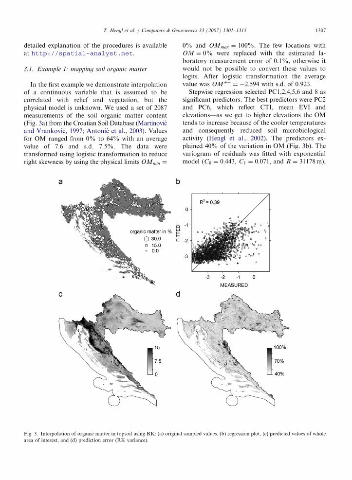
3.1. Example 1: mapping soil organic matter

In the first example we demonstrate interpolationof a continuous variable that is assumed to becorrelated with relief and vegetation, but thephysical model is unknown. We used a set of 2087measurements of the soil organic matter content(Fig. 3a) from the Croatian Soil Database (Martinovicand Vrankovic, 1997; Antonic et al., 2003). Valuesfor OM ranged from 0% to 64% with an averagevalue of 7.6 and s.d. 7.5%. The data weretransformed using logistic transformation to reduceright skewness by using the physical limits OMmin ¼

Fig. 3. Interpolation of organic matter in topsoil using RK: (a) origina

area of interest, and (d) prediction error (RK variance).

0% and OMmax ¼ 100%. The few locations withOM ¼ 0% were replaced with the estimated la-boratory measurement error of 0.1%, otherwise itwould not be possible to convert these values tologits. After logistic transformation the averagevalue was OMþþ ¼ �2:594 with s.d. of 0.923.

Stepwise regression selected PC1,2,4,5,6 and 8 assignificant predictors. The best predictors were PC2and PC6, which reflect CTI, mean EVI andelevations—as we get to higher elevations the OMtends to increase because of the cooler temperaturesand consequently reduced soil microbiologicalactivity (Hengl et al., 2002). The predictors ex-plained 40% of the variation in OM (Fig. 3b). Thevariogram of residuals was fitted with exponentialmodel (C0 ¼ 0:443, C1 ¼ 0:071, and R ¼ 31178m),

l sampled values, (b) regression plot, (c) predicted values of whole

ARTICLE IN PRESST. Hengl et al. / Computers & Geosciences 33 (2007) 1301–13151308

with a relatively high nugget to sill ratio. Althoughthe variogram model indicates poor predictivepossibilities, almost half of variation has beenexplained by the regression model. Such variogramsa typical effect of removing the feature-spacestructure: the remaining nugget is smaller or thesame as in the original variogram, but the total sill isreduced. In this case, the residuals showed abouttwo times smaller sill and about three times shorterrange of spatial correlation than the target variable(C0 ¼ 0:553, C1 ¼ 0:365, and R ¼ 84129m). Con-sequently, the RK prediction map (Fig. 3c) closelyfollows the map of elevation, with few hot-spots inregions where the residuals were high. Finally, theprediction model explained 64% of total variation.The remaining areas of high prediction error(Eq. (6)) can be seen in Fig. 3d. The map of theprediction error can be now used to locate

Fig. 4. Interpolation of occurrence of yew (Taxus baccata L.): (a) 3

(c) predicted values of whole area of interest, and (d) prediction error

additional samples and consider using either largersupport size or more detailed predictors.

3.2. Example 2: mapping presence/absence of yew

The second example is an interpolation of a binaryvariable: presence or absence of a plant species ineach grid cell, in this case yew (Taxus baccata L.).The result is the probability of occurrence (logistic-regression model), based on 364 sample plotsarranged in a regular grid, in which yew was eitherpresent or absent (Fig. 4a). This grid was acquiredfrom the on-line Flora Croatica database (Nikolicand Topic, 2005). In this case the predictorsaccounted for only 22% of total variation(Fig. 4b). The stepwise regression procedure selectedsix PCs ð2; 4; 5; 6; 8; 10Þ, the best predictor in factbeing CANH. This is probably because yew is a

64 observations on a regular grid, (b) logistic regression plot,

(RK variance).

ARTICLE IN PRESST. Hengl et al. / Computers & Geosciences 33 (2007) 1301–1315 1309

species that favours shady sites, e.g. areas of deepboreal forest. The variogram of residuals was fitted,as in previous case study, with an exponential model(C0 ¼ 4:126, C1 ¼ 5:336 and R ¼ 13797m). Again,the nugget variation was rather significant. Inaddition, the prediction error is rather high,indicating that only 46% of variation has beenexplained by the model (Fig. 4d). Note also fromFig. 4d that the prediction error mainly reflectsspatial location of points. The problem with thisdata set is obviously in the sampling design andsampling density. In this case, the short-rangevariation is completely under-sampled, the shortestspacing between the points is about 13 km and suchsampling density probably does not comply with thetargeted 200m grid resolution.

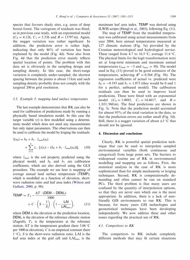
3.3. Example 3: mapping land surface temperature

The last example demonstrates that RK can also beused for calibration of predictions made by running aphysically based simulation model. In this case thetarget variable (z) is first modelled using a determi-nistic model which does not need any measurementsbut only input parameters. The observations can thenbe used to calibrate the model by kriging the residuals:

zðs0Þ ¼ b0 þ b1 � zmodðs0Þ

þXn

i¼1

li � ½zðsiÞ � ðb0 þ b1 � zmod ðs0ÞÞ�, ð10Þ

where zmod is the soil property predicted using thephysical model, and b0 and b1 are calibrationcoefficients, which are also derived using the GLSprocedure. The example we use here is mapping ofaverage annual land surface temperature (TEMP),which is modelled as a function of elevation, short-wave radiation ratio and leaf area index (Wilson andGallant, 2000, p. 98):

TEMP ¼ Tb �DT � ðDEM� DEMbÞ

1000

þ C � S �1

S

� �� 1�

LAI

LAImax

� �, ð11Þ

where DEM is the elevation at the prediction location,DEMb is the elevation of the reference climatic station(Zagreb), Tb is the temperature at the referencestation, DT is the temperature gradient (here 5:06 Cper 1000m elevation), C is an empirical constant (here1 C), S is the short-wave radiation ratio, LAI is theleaf area index at the grid cell and LAImax is the

maximum leaf area index. TEMP was derived usingILWIS scripts (Hengl et al., 2003), following Eq. (11).

The map of TEMP from the modelled tempera-ture was calibrated using actual measurements fromyear 2004, here annual temperatures measured at127 climatic stations (Fig. 5a) provided by theCroatian meteorological and hydrological service.These ranged from 4.7 to 16:5 C, average 11:6 C.The physical limits for the logit transformation wereset at long-term minimum and maximum annualtemperatures (zmin ¼ �5 and zmax ¼ 30). The modelused in Eq. (11) proved to be good estimator of thetemperatures, achieving R2 ¼ 0:564 (Fig. 5b). Theregression coefficients of actual vs. predicted wereb0 ¼ �0:193 and b1 ¼ 1:073 (they would be 0 and 1for a perfect, unbiased model). The calibrationresiduals can then be used to improve localpredictions. These were fitted with an exponentialmodel (C0 ¼ 1:0885, C1 ¼ 14:4617, and R ¼

1; 031; 960m). The final predictions are shown inFig. 5c. Note that the prediction model accountedfor almost 95% of the total variation in the data, sothat the prediction errors are rather small (Fig. 5d).Still, there is a nugget variation of about 1 C thatshould not be ignored.

4. Discussion and conclusions

Clearly, RK is powerful spatial prediction tech-nique that can be used to interpolate sampledenvironmental variables (both continuous andcategorical) from large point sets. The barriers towidespread routine use of RK in environmentalmodelling and mapping are as follows. First, thestatistical analysis in the case of RK is moresophisticated than for simple mechanistic or krigingtechniques. Second, RK is computationally de-manding and often cannot be run on standardPCs. The third problem is that many users areconfused by the quantity of interpolation options,so that they are never sure which one is the mostappropriate. In addition, there is a lack of user-friendly GIS environments to run RK. This isbecause, for many years GIS technologies andgeostatistical techniques have been developingindependently. We now address these and otherissues regarding the practical use of RK.

4.1. Competitors to RK

The competitors to RK include completelydifferent methods that may fit certain situations

ARTICLE IN PRESS

Fig. 5. Interpolation of land surface temperature: (a) original sampled values, (b) calibration plot, (c) predicted values of whole area of

interest, and (d) prediction error (RK variance).

T. Hengl et al. / Computers & Geosciences 33 (2007) 1301–13151310

better. If the auxiliary data are of different originand reliability, the Bayesian maximum entropyapproach might be a better alternative (D’Or,2003). There are also machine-learning techniquesthat combine neural network algorithms and robustinterpolators. Henderson et al. (2005) useddecision trees to predict various soil para-meters from large quantity of soil profile data andwith the help of land surface and remote sensingattributes. This technique is flexible, optimizes localfits and can be used within a GIS. However, it isstatistically suboptimal because it ignores spatiallocation of points during the derivation ofclassification trees. The same authors furtherreported (Henderson et al., 2005, pp. 394–396)that, although there is still some spatial correla-tion in the residuals, it is not clear how toemploy it.

RKmust also be compared with alternative krigingtechniques, such as OK and cokriging (CK). Theadvantage of OK is that it is less complicated in itsuse and included in most software packages. How-ever, when auxiliary information is available in theform of maps of covariates that can explain part ofthe variation in the target variable, then RK outper-forms OK because it exploits the extra information.Colocated CK does make use of the auxiliaryinformation, but is developed for situations in whichthe auxiliary information is not spatially exhaustive(Knotters et al., 1995). CK also requires simultaneousmodelling of both direct and cross variograms, whichcan be time-consuming for large number of covari-ates. In the case where the covariates are available asmaps, RK will generally be preferred over CK,although CK may in some circumstances give super-ior results (Goovaerts, 1999).

ARTICLE IN PRESS

Table

1

ComparisonofcomputingcapabilitiesofsomepopularstatisticalandGIS

packages

(versionsin

year2005)

Aspect

S-

PLUS

GSTAT/

R

SURFER

ISATIS

GEOEasGSLIB

GRASSPC

Raster

ILWIS

IDRISIArcGIS

SAGA

Commercialprice

category

IIIV

III

IIV

IVIV

III

IVII

IIV

Main

application

A,B

BB,E

BB

BB,C

CB,C

B,C

B,E

B,C

User-friendly

environmentto

non-expert

$�

$$

��

%�

$$

$$

Quality

ofsupport

anddescriptionofalgorithms

%$

%$

$$

%%

$$

%%

Standard

GIS

capabilities

�%

%�

��

$%

$$

$$

Standard

descriptivestatisticalanalysis

$$

�$

%%

%�

$$

$%

Imageprocessingtools(orthorectification,filtering,landsurface

analysis)�

��

��

�%

�$

$%

$

Comprehensiveregressionanalysis(regressiontrees,GLM)

$$

�%

��

��

�%

��

Interactive(automated)variogram

modelling

�$

�$

�%

��

�$

$�

Regression-krigingwithauxiliary

maps

�$

�%

��

$%

%$

�$

Dynamic

modelling(sim

ulations,spatialiterations,propagation,

anim

ations)

�%

��

��

%$

%%

%%

$—

Fullcapability,%—possiblebutwithmanylimitations,�—notpossiblein

thispackage.Commercialprice

category:I—

41000EUR;II—

500–1000EUR;III—

o500EUR;IV

—

open

sourceorfreeware.Main

application:A—statisticalanalysisanddata

mining;B—interpolationofpointdata;C—processingofauxiliary

maps;E—preparationandvisualization

offinalmaps.

T. Hengl et al. / Computers & Geosciences 33 (2007) 1301–1315 1311

4.2. Software implementation

There is still a large gap between what is possiblefor some (researchers) and what is available to many(users). No GIS package includes all of generalizedlinear models, variogram fitting, iterative estimationof residual variograms, and kriging, let alone theirseamless integration. We have compared differentaspects of geostatistical packages listed by the AI-GEOSTATS group (http://ai-geostats.org) and several well-known GIS packages (Table 1,see also supplementary materials at http://spatial-analyst.net). Although the UK(using coordinates) is available in most geostatis-tical packages, KED with multiple auxiliary mapscan be run in only a limited number of packages. Infact, only Isatis (http://geovariances.com),SAGA (http://saga-gis.org), and GSTAT(http://-gstat.org) as stand-alone applica-tion or integrated into R (R Development CoreTeam, 2004; Pebesma, 2004), GRASS (http://geog.uni-hannover.de/grass) or Idrisi(http://clarklabs.org) offer a possibility tointerpolate a variable using auxiliary maps. We havetested RK in all these packages to discover that RKin Isatis is limited to a use of a single (three in scriptmode) auxiliary maps (Bleines et al., 2005). In IdrisiGLS regression coefficients cannot be estimated andthe system is rather unstable. In GSTAT, both RKpredictions and simulations (predictors as basemaps) at both point and block support can be runby defining short scripts, which can help automatizeinterpolation of large amounts of data. However,GSTAT implements the algorithm with extendedmatrix (KED), which means that both the values ofpredictors and of target variable are used toestimate the values at each new location, whichfor large data sets can by time-consuming or canlead to computational problems (Leopold et al.,2005).

Setting UK in GSTAT to a smaller windowsearch can lead to termination of the program dueto the singular matrix problems. In fact, local UKwith a global variogram model is not valid becausethe regression model will differ locally, hence thealgorithm should also estimate the variogram modelfor residuals for each local neighbourhood. Thesingular matrix problem will happen especiallywhen indicator variables are used as predictors orif the two predictor maps are highly correlated. Ourexperience with GSTAT was that interpolation ofmore than 1000 points over 1M of pixels can last up

ARTICLE IN PRESST. Hengl et al. / Computers & Geosciences 33 (2007) 1301–13151312

to several hours on a standard PC. To runsimulations in GSTAT with the same settings willtake even more time. This clearly proves that,although KED procedure is mathematically elegant,such problems show that it might be more effectivefor real-life applications to fit the trend andresiduals separately (RK) instead of through useof an extended matrix (KED). Another limitation ofGSTAT is that it is a stand-alone application andthe algorithms cannot be adjusted easily.

To allow extension of GSTAT functionalities andintegration of its functionalities with other statis-tical functions, the developer of GSTAT, with asupport of colleagues, developed an R packagecalled spatial (http://r-spatial.source-forge.net). R itself provides rich facilities forregression modelling, including GLS. The onlyproblem here is that each step must be run by theanalyst, who must really be an R expert. The open-source packages open the door to analyses ofunlimited sophistication. However, they were notdesigned with graphical user interface, wizards, orinteraction as is typical for commercial GIS, so arenot easily used by non-experts. There is thusopportunity both for commercial GIS to incorpo-rate RK ideas, or for open-source software tobecome more user-friendly.

4.3. Limitations of RK

Finally, there are some limitations to routine useof RK. If any of these problems occur, RK can giveeven worse results than even non-statistical, empiri-cal interpolators such as Thiessen polygons ormoving averages. The following difficulties mightalso be considered as challenges for the geostatisti-cians:

(1)

Data quality: RK relies completely on thequality of data. If the data comes from differentsources and have been sampled using biased orunrepresentative design, the predictions mightbe even worse than with simple mechanisticprediction techniques (Example 2, Fig. 4). Evena single bad data point can make any regressionarbitrarily bad, which affects the RK predictionover the whole area.

(2)

Under-sampling: For regression modelling, themultivariate feature space must be well-repre-sented in all dimensions. For variogram model-ling, an adequate number of point-pairs must beavailable at various spacings. Webster and

Oliver (2001, p. 85) recommend at least 50 andpreferably 300 points for variogram estimation.Neter et al. (1996) recommends at least 10observations per predictor for multiple regres-sion. We strongly recommend using RK only fordata sets with more than 50 total observationsand at least 10 observations per predictor toprevent over-fitting.

(3)

Reliable estimation of the covariance/correlation

structure: The major dissatisfaction of usingKED or RK is that both the regression modelparameters and covariance function parametersneed to be estimated simultaneously. However,in order to estimate coefficients we need to knowcovariance function of residuals, which can onlybe estimated after the coefficients (the chick-en–egg problem). Here, we have assumed that asingle iteration is a satisfactory solution,although someone might also look for otheriterative solutions (Kitanidis, 1994).

(4)

Extrapolation outside the sampled feature space:If the points do not represent feature space orrepresent only the central part of it, this willoften lead to poor estimation of the model andpoor spatial prediction (Example 1, Fig. 4d).This is especially important for linear modellingwhere the prediction variance exponentiallyincreases as we get closer to the edges of thefeature space. For this reason it is importantthat the points be well spread at the edges of thefeature space and that they be symmetricallyspread around the center of the feature space(Hengl et al., 2004c). An assessment of theextrapolation in feature space can also be usedto allocate additional point samples that can beused to improve the existing prediction models.This also justifies use of multiple predictors to fitthe target variable, instead of using only the mostsignificant predictor or first principal com-ponent, which is, for example, advocated bythe Isatis development team (Bleines et al.,2005).

(5)

Predictors with uneven relation to the target

variable: Auxiliary maps should have a constantphysical relationship with the target variable inall parts of the study area, otherwise artefactswill be produced. An example is a single NDVIas a predictor of topsoil organic matter. If anagricultural field has just been harvested (lowNDVI), the prediction map will (incorrectly)show very low organic matter content within thecrop field.

ARTICLE IN PRESST. Hengl et al. / Computers & Geosciences 33 (2007) 1301–1315 1313

(6)

Intermediate-scale modelling: RK has not beenadapted to fit data locally, with arbitraryneighbourhoods for the regression as can bedone with kriging with moving window (Walteret al., 2001). Many practitioners would like toadjust the neighbourhood to fit their concepts ofthe scale of processes that are not truly global(across the whole study area) but not fully localeither.

4.4. Next steps

What the programmers might consider for futureis the refinement of (local) RK in a moving window.This will allow not only better data fitting, but willalso allow users to visualize variation in regression(maps of R2 and regression coefficients) andvariogram models (maps of variogram parameters).Note that the RK with moving window would needto be fully automated, which might not be an easytask considering the computational complexity.Also, unlike the OK with moving window (Walteret al., 2001), RK has much higher requirementsconsidering the minimum number of observations(at least 10 per predictor, at least 50 to modelvariogram). In general, our impression is that muchof the procedures (regression and variogram model-ling) in RK can be automated and amount of datamodelling definitions expanded (local or globalmodelling, transformations, selection of predictors,type of GLMs etc.), as long as the point data set islarge and of high quality. Ideally, the user should beable to easily test various combinations of inputparameters and then (in real-time) select the onethat produces most satisfactory predictions.

In conclusion, RK is a flexible method formodelling and mapping which offers conceptualadvantages over alternative methods. We hope itbecomes a routine part of the geostatistical toolbox.A task for the programmers in the near future willbe to incorporate statistical procedures, such asstep-wise regression, neural networks, automatedvariogram modelling, simulated annealing, unsu-pervised fuzzy classification and similar, within GISuser environments. Because many statistical techni-ques can be automated, integration of GIS andstatistical algorithms should open the possibility toeasily and quickly interpolate dozens of variables byusing dozens of predictors. Nevertheless, analystsshould have the final control to adjust the system asneeded. To do this, they should have full insight intoalgorithms used.

Appendix A. Proof of equivalence of RK and KED

Start from kriging with external drift (or universalkriging) where the predictions are made as in OKusing zKEDðs0Þ ¼ kTKED � z. The KED krigingweights (lTKED) are obtained by solving the system(Wackernagel, 1998, p. 179):

C q

qT 0

" #�

kKED

/

" #¼

c0

q0

" #, (A.1)

where / is a vector of Lagrange multipliers. Writingthis out yields:

C � kKED þ q � / ¼ c0,

qT � kKED ¼ q0. ðA:2Þ

From this follows:

qT � kKED ¼ qT � C�1 � c0 � qT � C�1 � q � / (A.3)

and hence:

/ ¼ ðqT � C�1 � qÞ�1 � qT � C�1 � c0

� ðqT � C�1 � qÞ�1 � q0, ðA:4Þ

where the identity qT � kKED ¼ q0 has been used.Substituting / back into Eq. (A.2) shows that theKED weights equal (Papritz and Stein, 1999, p. 94):

kKED ¼ C�1 � c0 � C�1 � q

� ½ðqT � C�1 � qÞ�1 � qT � C�1 � c0

� ðqT � C�1 � qÞ�1 � q0�

¼ C�1 � ½c0 þ q � ðqT � C�1 � qÞ�1

� ðq0 � qT � C�1 � c0Þ�. ðA:5Þ

Let us now turn to RK. Recall from Eq. (4) that theGLS estimate for the vector of regression coeffi-cients is given by

bGLS ¼ ðqT � C�1 � qÞ�1 � qT � C�1 � z (A.6)

and weights for residuals by

kT0 ¼ cT0 � C�1. (A.7)

Substituting these in RK formula (Eq. (5)) gives

zRKðs0Þ ¼ qT0 � bGLS þ kT0 � ðz� q � bGLSÞ

¼ ½qT0 � ðqT � C�1 � qÞ�1 � qT � C�1 þ cT0 � C

�1

� cT0 � C�1� q � ðqT � C�1qÞ�1 � qT � C�1� � z

ARTICLE IN PRESST. Hengl et al. / Computers & Geosciences 33 (2007) 1301–13151314

¼ C�1 � ½cT0 þ qT0 � ðqT � C�1 � qÞ�1 � qT

� cT0 � C�1� q � ðqT � C�1qÞ�1 � qT� � z

¼ C�1 � ½c0 þ q � ðqT � C�1 � qÞ�1

� ðq0 � qT � C�1c0Þ� � z. ðA:8Þ

The left part of the equation is equal to Eq. (A.5),which proves that KED will give the same predic-tions as RK if same inputs are used. A detailedcomparison of RK and KED is also available assupplementary material.

References

Ahmed, S., de Marsily, G., 1987. Comparison of geostatistical

methods for estimating transmissivity using data on trans-

missivity and specific capacity. Water Resources Research 23

(9), 1717–1737.

Antonic, O., Pernar, N., Jelaska, S., 2003. Spatial distribution of

main forest soil groups in croatia as a function of basic

pedogenetic factors. Ecological Modelling 170 (2–3),

363–371.

Berterretche, M., Hudak, A.T., Cohen, W.B., Maiersperger,

T.K., Gower, S.T., Dungan, J., 2005. Comparison of

regression and geostatistical methods for mapping leaf area

index (LAI) with landsat ETMþ data over a boreal forest.

Remote Sensing of Environment 96 (3), 49–61.

Bishop, T., McBratney, A., 2001. A comparison of prediction

methods for the creation of field-extent soil property maps.

Geoderma 103 (1–2), 149–160.

Bleines, C., Perseval, S., Rambert, F., Renard, D., Touffait, Y.,

2005. ISATIS. Isatis Software Manual. Geovariances & Ecole

Des Mines De, Paris, 710pp.

Bourennane, H., King, D., 2003. Using multiple external drifts to

estimate a soil variable. Geoderma 114 (1–2), 1–18.

Burrough, P., McDonnell, R., 1998. Principles of Geographical

Information Systems. Oxford University Press, Oxford,

333pp.

Chiles, J., Delfiner, P., 1999. Geostatistics: Modeling Spatial

Uncertainty. Wiley, New York, 695pp.

Christensen, R., 1996. Plane Answers to Complex Questions: The

Theory of Linear Models, second ed. Springer, New York,

452pp.

Christensen, R., 2001. Linear Models for Multivariate Time

Series and Spatial Data, second ed. Springer, New York,

398pp.

Cressie, N., 1993. Statistics for Spatial Data, revised ed. Wiley,

New York, 900pp.

Desbarats, A.J., Logan, C.E., Hinton, M.J., Sharpe, D.R., 2002.

On the kriging of water table elevations using collateral

information from a digital elevation model. Journal of

Hydrology 255 (1–4), 25–38.

Deutsch, C., Journel, A., 1998. GSLIB: Geostatistical Software

and User’s Guide, second ed. Oxford University Press, New

York, 369pp.

Dobos, E., Micheli, E., Baumgardner, M.F., Biehl, L., Helt, T.,

2000. Use of combined digital elevation model and satellite

radiometric data for regional soil mapping. Geoderma 97

(3–4), 367–391.

D’Or, D., 2003. Spatial Prediction of Soil Properties, the

Bayesian Maximum Entropy Approach. Ph.D., Universite

Catholique de Louvain, 212pp.

Draper, N., Smith, H., 1981. Applied Regression Analysis,

second ed. Wiley, New York, 709pp.

Finke, P.A., Brus, D.J., Bierkens, M.F.P., Hoogland, T.,

Knotters, M., de Vries, F., 2004. Mapping groundwater

dynamics using multiple sources of exhaustive high resolution

data. Geoderma 123 (1–2), 23–39.

Goovaerts, P., 1997. Geostatistics for Natural Resources

Evaluation. Oxford University Press, New York, 483pp.

Goovaerts, P., 1999. Using elevation to aid the geostatistical

mapping of rainfall erosivity. Catena 34 (3–4), 227–242.

Gotway, C., Stroup, W., 1997. A generalized linear model

approach to spatial data analysis and prediction. Journal of

Agricultural, Biological, and Environmental Statistics 2 (2),

157–198.

Henderson, B., Bui, E., Moran, C., Simon, D., 2005. Australia-

wide predictions of soil properties using decision trees.

Geoderma 124 (3–4), 383–398.

Hengl, T., 2006. Finding the right pixel size. Computers &

Geosciences 32 (9), 1283–1298.

Hengl, T., Rossiter, D.G., Husnjak, S., 2002. Mapping soil

properties from an existing national soil data set using freely

available ancillary data. In: Proceedings of the 17th World

Congress of Soil Science, Paper no. 1140. IUSS, Bangkok,

Thailand, p. 1481.

Hengl, T., Gruber, S., Shrestha, D., 2003. Digital Terrain

Analysis in ILWIS. Lecture Notes. International Institute

for Geo-Information Science & Earth Observation (ITC),

Enschede, 56pp.

Hengl, T., Gruber, S., Shrestha, D.P., 2004a. Reduction of errors

in digital terrain parameters used in soil–landscape modelling.

International Journal of Applied Earth Observation and

Geoinformation (JAG) 5 (2), 97–112.

Hengl, T., Heuvelink, G., Stein, A., 2004b. A generic framework

for spatial prediction of soil variables based on regression-

kriging. Geoderma 122 (1–2), 75–93.

Hengl, T., Rossiter, D., Stein, A., 2004c. Soil sampling

strategies for spatial prediction by correlation with auxiliary

maps. Australian Journal of Soil Research 41 (8),

1403–1422.

Kellndorfer, J., Walker, W., Pierce, L., Dobson, C., Fites, J.A.,

Hunsaker, C., Vona, J., Clutter, M., 2004. Vegetation height

estimation from shuttle radar topography mission and

national elevation datasets. Remote Sensing of Environment

93 (3), 339–358.

Kitanidis, P., 1994. Generalized covariance functions in estima-

tion. Mathematical Geology 25, 525–540.

Knotters, M., Brus, D., Voshaar, J., 1995. A comparison of

kriging, co-kriging and kriging combined with regression for

spatial interpolation of horizon depth with censored observa-

tions. Geoderma 67 (3–4), 227–246.

Leopold, U., Heuvelink, G.B., Tiktak, A., Finke, P.A., Schou-

mans, O., 2005. Accounting for change of support in spatial

accuracy assessment of modelled soil mineral phosphorous

concentration. Geoderma 130 (3–4), 368–386.

Lloyd, C.D., 2005. Assessing the effect of integrating elevation

data into the estimation of monthly precipitation in Great

Britain. Journal of Hydrology 308 (1–4), 128–150.

Lopez-Granados, F., Jurado-Exposito, M., Pena-Barragan, J.,

Garcia-Torres, L., 2005. Using geostatistical and remote

ARTICLE IN PRESST. Hengl et al. / Computers & Geosciences 33 (2007) 1301–1315 1315

sensing approaches for mapping soil properties. European

Journal of Agronomy 23 (33), 279–289.

Martinovic, J., Vrankovic, A. (Eds.), 1997. Croatian Soil

Database (in Croatian), vols. I–III, Ministry of Environ-

mental Protection and Physical Planning, Zagreb.

Matheron, G., 1969. Le krigeage universel (Universal kriging).

vol. 1. Cahiers du Centre de Morphologie Mathematique,

Ecole des Mines de Paris, Fontainebleau, 83pp.

McKenzie, N., Ryan, P., 1999. Spatial prediction of soil

properties using environmental correlation. Geoderma 89

(1–2), 67–94.

Neter, J., Kutner, M., Nachtsheim, C., Wasserman, W. (Eds.),

1996. Applied Linear Statistical Models, fourth ed. McGraw-

Hill/Irwin, Chicago, New York, 1408pp.

Nikolic, T., Topic, J. (Eds.), 2005. Red Book of Vascular Flora of

Croatia. Ministry of Culture, State Institute for Nature

Protection, Republic of Croatia, Zagreb, 693pp.

Odeh, I., McBratney, A., Chittleborough, D., 1995. Further

results on prediction of soil properties from terrain attributes:

heterotopic cokriging and regression-kriging. Geoderma 67

(3–4), 215–226.

Papritz, A., Stein, A., 1999. Spatial prediction by linear kriging.

In: Stein, A., van der Meer, F., Gorte, B. (Eds.), Spatial

Statistics for Remote Sensing. Kluwer Academic Publishers,

Dodrecht, pp. 83–113.

Pebesma, E.J., 2004. Multivariable geostatistics in S: the gstat

package. Computers & Geosciences 30 (7), 683–691.

Pleydell, D.R.J., Raoul, F., Tourneux, F., Danson, F.M.,

Graham, A.J., Craig, P.S., Giraudoux, P., 2004. Modelling

the spatial distribution of Echinococcus multilocularis infec-

tion in foxes. Acta Tropica 91 (3), 253–265.

R Development Core Team, 2004. R: A Language and

Environment for Statistical Computing. R Foundation for

Statistical Computing, Vienna, Austria, ISBN 3-900051-00-3.

Rabus, B., Eineder, M., Roth, A., Bamler, R., 2003. The

shuttle radar topography mission—a new class of digital

elevation models acquired by spaceborne radar. ISPRS

Journal of Photogrammetry and Remote Sensing 57 (4),

241–262.

Rivoirard, J., 2002. On the structural link between variables in

kriging with external drift. Mathematical Geology 34 (7),

797–808.

Wackernagel, H., 1998. Multivariate Geostatistics: An Introduc-

tion with Applications, second ed. Springer, Berlin, 291pp.

Walter, C., McBratney, A.B., Donuaoui, A., Minasny, B., 2001.

Spatial prediction of topsoil salinity in the Chelif valley,

Algeria, using local ordinary kriging with local variograms

versus whole-area variogram. Australian Journal of Soil

Research 39, 259–272.

Webster, R., Oliver, M., 2001. Geostatistics for Environmental

Scientists Statistics in Practice. Wiley, Chichester,

271pp.

Wilson, P.J., Gallant, C.J. (Eds.), 2000. Terrain Analysis:

Principles and Applications. Wiley, New York, 479pp.

Yemefack, M., Rossiter, D.G., Njomgang, R., 2005. Multi-scale

characterization of soil variability within an agricultural

landscape mosaic system in southern Cameroon. Geoderma

125 (1–2), 117–143.