This is an electronic reprint of the original article.This reprint may differ from the original in pagination and typographic detail.

Powered by TCPDF (www.tcpdf.org)

This material is protected by copyright and other intellectual property rights, and duplication or sale of all or part of any of the repository collections is not permitted, except that material may be duplicated by you for your research use or educational purposes in electronic or print form. You must obtain permission for any other use. Electronic or print copies may not be offered, whether for sale or otherwise to anyone who is not an authorised user.

Abed, Ayman; Korkiala-Tanttu, Leena; Forsman, Juha; Koivisto, Kirsi3D Simulations of Deep Mixed Columns under Road Embankment

Published in:Rakenteiden Mekaniikka - Journal of Structural Mechanics

Published: 01/01/2021

Document VersionPublisher's PDF, also known as Version of record

Published under the following license:CC BY

Please cite the original version:Abed, A., Korkiala-Tanttu, L., Forsman, J., & Koivisto, K. (2021). 3D Simulations of Deep Mixed Columns underRoad Embankment. Rakenteiden Mekaniikka - Journal of Structural Mechanics, 54(1), 1-20.https://rakenteidenmekaniikka.journal.fi/article/view/84590

1Corresponding author: ayman.abed@chalmers.se

1

Rakenteiden Mekaniikka (Journal of Structural Mechanics)

Vol. 54, No. 1, 2021, pp. 1–20

http://rakenteidenmekaniikka.journal.fi/index

https://doi.org/10.23998/rm.84590

© 2020 The Authors

Open access under license CC BY 4.0

3D simulations of deep mixed columns under road

embankment

Ayman Abed1, Leena Korkiala-Tanttu, Juha Forsman and Kirsi Koivisto

Summary When column stabilisation is meant to function as a ground improvement under an

embankment, the design cases to be considered consist of overall stability, compression resistance

of the column heads, arching of the embankment on the columns and settlements. This paper

focuses on the compression resistance of the columns. The proper geotechnical design of deep

mixed (deep stabilised) columns under road embankment requires good estimation of the stress-

strain behaviour of the columns and the surrounding soil under the embankment and traffic

loading. Earlier Finnish design approaches relied on an even traffic load of 10 kN/m2 on the road

surface. The dimensioning methods for column stabilised soil are also based on the idea of an

even traffic load. Due to Eurocode recommendations a more realistic scenario is introduced,

which remarkably increases the magnitude of the traffic loading. After deriving suitable material

properties and stiffness parameters for static and dynamic traffic loading, three-dimensional finite

element calculations are performed to achieve better understanding of the mechanical interaction

between the embankment, columns and soil under the new loading configuration. Even though

more investigations are needed before delivering a final statement, the calculations show that, for

the considered case in this paper, the new loading scenario has no relevant consequences on the

design compared to the earlier design approach.

Key words: soil stabilisation, finite-element modelling, dynamic loading.

Received: 20 August 2019. Accepted: 5 August 2020. Published online: 20 January 2021.

Introduction

Deep mixing or deep stabilisation is a widely used ground improvement method in

Finland in areas of soft clay [10]. Especially the use of columns made with the dry mixing

method has established its role in Nordic foundation engineering [30]. In column

stabilisation, a mixing head is pushed and rotated though the soft subsoil into the desired

depth. Then it is raised up by rotating while simultaneously adding binder material

pneumatically into the soil [5]. After a curing time, typically from one to three months,

2

the hardened columns and surrounding soft soil between the columns create an

inhomogeneous soil mass, where in the long-term stresses concentrate mainly on the

columns.

Finnish Transport Agency (FTA) has updated the guidelines for the design of deep

mixing [7]. The implementation of the Eurocode approach with new traffic loads was the

main drive behind updating the earlier guidelines from 2010 [9]. FTA substantially

updated the traffic loads for roads in their guideline NCCI7 [8]. The loads presented in

“Geotechnical Design, Application guidelines for Eurocode in Finnish FTA’s guideline

NCCI7” [8] are based on the measurements made on the Finnish road network during

2013 and 2014 [29]. Earlier, the design traffic load for roads [6, 9] was an evenly

distributed 10 kN/m2. According to the new regulations the traffic load became an evenly

distributed load of 9 kN/m2 with an additional distributed load of 31 kN/m2 at the area of

3 m x 5 m on one lane. The location of this additional load can vary (Figure 1).

Figure 1. Top view of the traffic load for road design according to NCCI7 [8].

Broms and Boman [3] presented the design principles of elastic columns based on the

concept of equal strain of columns and soil. The elastic column means that in the design

the yield stress of columns, assumed to be 70 % of the failure strength, is not exceeded.

The design of the columns is based on the allowed load of the column. The design method

applies a long-term modulus for the columns and the soft soil between columns [7, 9].

The earlier design guidelines adopted the analytical method of linear elasticity [23] to

estimate the stress distribution between columns and the surrounding soil [9, 3]. The 10

kN/m2 even traffic loading was assumed not to be distributed in the embankment or in

the dry crust layer.

In the case of an additional distributed loading of 31 kN/m2 (on an area of 3 m x 5 m)

the load is assumed to be distributed in the embankment. The stress distribution in the

embankment and subsoil layers was simulated for both the uniform loading of 10 kN/m2

and the updated traffic loading. The comparison showed a clear increase of the stress level

for the 31 kPa loading in the upper part of the column compared to the previously

implemented loading of 10 kPa. This increase would directly affect the design, and the

centre-to-centre (c/c) distance for the elastic columns would decrease (or the diameter of

the columns or the binder amount would increase) leading to more expensive deep mixing

for the embankment foundation. However, the existing deep mixed column structures

have performed quite well, and during the last 40 years only in few cases have problems

3

been reported in the existing column structures. In some of these cases, no dry crust layer

has existed and the embankment has been thin, so the traffic load at the uppermost part

of the column has exceeded the yield stress level.

Based on the simulations made during updating the guidelines, it was found that the

new distributed traffic load and the earlier dimensioning method cannot be combined

before more consideration is done. In the simulations, the old even traffic load of 10 kPa

was replaced by a new distributed load, which in analytical calculations gives somewhat

overconservative results. To find a solution to this issue, versatile three-dimensional

numerical simulations are done. The objective of this paper is to present and discuss the

results of three-dimensional simulations of a road embankment over column-stabilised

soil that is subjected to a traffic load configuration which meets the new design guidelines.

Implicitly, the paper proposes a method to define the material parameters for similar

loading scenarios. On the grounds of the numerical results, the paper delivers

recommendations for improving the current design practice of such cases.

Problem geometry

Figure 2 illustrates the road cross section, its dimensions, columns and the subsoil in 3D

space. The dimensions of the embankment correspond to a fairly conventional Finnish

case of column stabilisation as a ground improvement method. The height of the

embankment is 2 meters, the width 10 meters and the inclination of slopes 1:2. The subsoil

has two layers: i) dry crust which is a thin, relatively strong partially saturated clay layer

that lies directly over a soft saturated clay layer. In Finland the typical thickness of dry

crust is 0.5 to 3 meters. The current study considers an average thickness of 1 meter. The

current study considers an average thickness of 1 meter ii) soft clay of 10 meters. Below,

there is a stiff soil layer (moraine). The soft clay has the typical properties for a coastal

Finland clay. Two column spacings were chosen with the centre-to-centre (c/c) distances

of 0.9 m and 1.3 m, and a diameter of 600 mm for the columns. The columns were of two

different types, soft and stiff. The diameter, c/c distance and the strength of the elastic

columns were selected according to analytical calculations done following the guidelines

of FTA (2010) [9] with the evenly distributed traffic load of 10 kN/m2.

The stress distributions were mainly analysed on the bottom of the dry crust and along

the column in the middle of the road (see the red rectangle in Figure 2). This area is

normally the most critical part of the column in the compression strength design. The

columns were assumed to behave as an elastic material.

When the columns are elastic, the embankment load is distributed over the columns

and subsoil in relation to their area-weighted stiffness. About 90–95% of the embankment

load is typically distributed to the columns.

4

Figure 2. Problem geometry. Distance between the columns (D = 600 mm) is c/c = 0.9 or

1.3 m. The stress distributions were mainly analysed at the bottom of the dry crust and along the

column in the middle of the road and subsoil – see the red rectangle.

Parameters in different design situations

The compression resistance of the columns should be analysed e.g. in the following two

cases:

1. Final embankment and pavement structure + dynamic traffic load.

2. Final embankment and pavement structure + a static live load (e.g. truck

parking area).

Case 1 is the most common, where the stress caused by the fast-acting (dynamic)

traffic load is passed to the columns, to the granular structure of the soil between columns

and to the generated excess pore pressure. Whereas, under the static load, the excess pore

pressure has time to partly dissipate, and a greater portion of the load concentrates on the

columns and the granular structure of the soil between columns than in the case of the

dynamic load. This article mainly discusses case 1, however the soil parameters are

derived for both cases.

The previous design guidelines [9] used stiffness modulus Ecol for columns and

drained state tangent modulus M for soil. The modelling with dynamic traffic load,

presented in this paper, uses initial undrained stiffness modulus Eu,col0 for columns and

Eu,soil0 for the soil between columns. To define the initial stress state equivalent to the

embankment load, drained Young’s modulus E' is used for the soil between columns and

Ecol for columns. Only linear elastic material models are employed in the current FEM

modelling.

It is worth mentioning that when modelling the structure with the static load, drained

elastic modulus E0 was employed for the soil between columns. Even though the

modelling of this case is not presented here but the needed parameters are provided in the

following section.

5

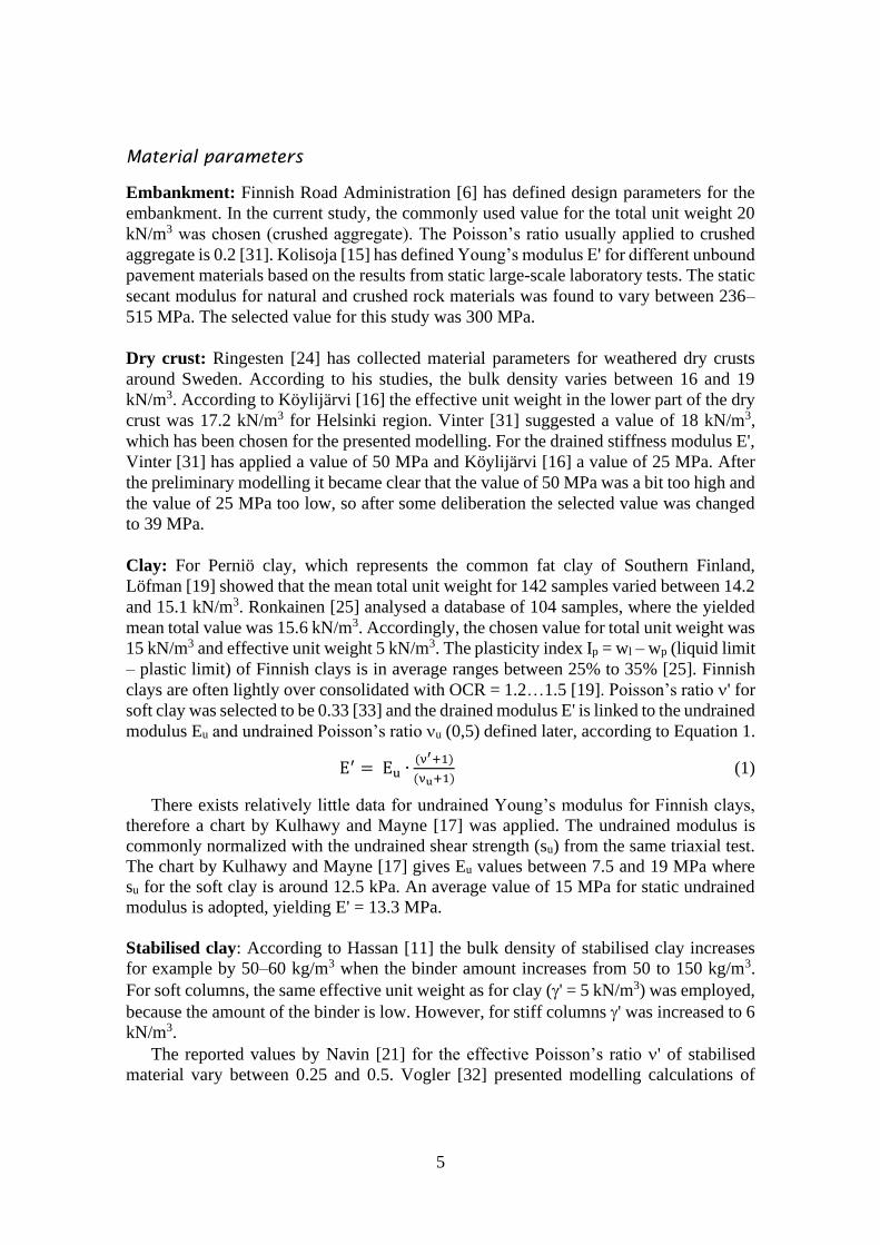
Material parameters

Embankment: Finnish Road Administration [6] has defined design parameters for the

embankment. In the current study, the commonly used value for the total unit weight 20

kN/m3 was chosen (crushed aggregate). The Poisson’s ratio usually applied to crushed

aggregate is 0.2 [31]. Kolisoja [15] has defined Young’s modulus E' for different unbound

pavement materials based on the results from static large-scale laboratory tests. The static

secant modulus for natural and crushed rock materials was found to vary between 236–

515 MPa. The selected value for this study was 300 MPa.

Dry crust: Ringesten [24] has collected material parameters for weathered dry crusts

around Sweden. According to his studies, the bulk density varies between 16 and 19

kN/m3. According to Köylijärvi [16] the effective unit weight in the lower part of the dry

crust was 17.2 kN/m3 for Helsinki region. Vinter [31] suggested a value of 18 kN/m3,

which has been chosen for the presented modelling. For the drained stiffness modulus E',

Vinter [31] has applied a value of 50 MPa and Köylijärvi [16] a value of 25 MPa. After

the preliminary modelling it became clear that the value of 50 MPa was a bit too high and

the value of 25 MPa too low, so after some deliberation the selected value was changed

to 39 MPa.

Clay: For Perniö clay, which represents the common fat clay of Southern Finland,

Löfman [19] showed that the mean total unit weight for 142 samples varied between 14.2

and 15.1 kN/m3. Ronkainen [25] analysed a database of 104 samples, where the yielded

mean total value was 15.6 kN/m3. Accordingly, the chosen value for total unit weight was

15 kN/m3 and effective unit weight 5 kN/m3. The plasticity index Ip = wl – wp (liquid limit

– plastic limit) of Finnish clays is in average ranges between 25% to 35% [25]. Finnish

clays are often lightly over consolidated with OCR = 1.2…1.5 [19]. Poisson’s ratio ' for

soft clay was selected to be 0.33 [33] and the drained modulus E' is linked to the undrained

modulus Eu and undrained Poisson’s ratio u (0,5) defined later, according to Equation 1.

E′ = Eu ∙(ν′+1)

(νu+1) (1)

There exists relatively little data for undrained Young’s modulus for Finnish clays,

therefore a chart by Kulhawy and Mayne [17] was applied. The undrained modulus is

commonly normalized with the undrained shear strength (su) from the same triaxial test.

The chart by Kulhawy and Mayne [17] gives Eu values between 7.5 and 19 MPa where

su for the soft clay is around 12.5 kPa. An average value of 15 MPa for static undrained

modulus is adopted, yielding E' = 13.3 MPa.

Stabilised clay: According to Hassan [11] the bulk density of stabilised clay increases

for example by 50–60 kg/m3 when the binder amount increases from 50 to 150 kg/m3.

For soft columns, the same effective unit weight as for clay (' = 5 kN/m3) was employed,

because the amount of the binder is low. However, for stiff columns ' was increased to 6

kN/m3.

The reported values by Navin [21] for the effective Poisson’s ratio ' of stabilised

material vary between 0.25 and 0.5. Vogler [32] presented modelling calculations of

6

stabilised soil with ' = 0.35 for the columns. An average value of 0.33 was adopted for

the current modelling. Determining the stiffness of stabilised soil is challenging and

therefore it is common to use empirical correlations between the undrained shear strength

of stabilised soil su,col and the related stiffness. Timoney [28] collected a list of these

equations to estimate the stiffness Ecol both from laboratory and field tests. Many of the

equations are linear and, for the most part, quite similar to each other. One of the more

common ones is Equation 2, which was also used in the old Finnish guide book [6].

Ecol = 100 ~ 200 ∙ su,col (2)

where su,col is estimated in [kPa].

According to Swedish Road Administration [27] the stiffness modulus for columns

Ecol can be derived from Equation 3, where 0.7 x su,col represents the value of the shear

yielding strength for the stabilised soil of columns. In both the new and the former Finnish

guidelines [7, 9], the column stiffness is derived based on Equation 4.

Ecol = 13 (0.7 su,col)1.6

(3)

Ecol = 20 (0.7 su,col)1.6

(4)

To make the design cases as realistic as possible, it was assumed that the “soft”

columns and the “stiff” columns have the shear strengths of 70 kPa and 150 kPa,

respectively. Consequently, based on Equations 2 and 4 taken from Finnish handbooks,

the nominal values of column stiffness are 7–14 MPa (Eq. 2) or 10 MPa (Eq. 4) for the

“soft” columns and 15–30 or 34 MPa for the “stiff” columns. Table 1 shows the literature

values and the selected material parameters. The stiffness parameters in this table are used

for modelling the case of static traffic loading (not presented in this paper).

Table 1. Material parameters. Literature values / selected values.

Material Unit weight '

[kN/m3]

Drained Poisson’s

ratio ' [-]

Drained Young’s

modulus E' [MPa]

Embankment 20 / 20 0.21 / 0.2 236–5152 / 300

Dry crust 181 / 18 0.31 / 0.3 259–502 / 39

Clay, soft 14.2–15.13 / 15 0.334 /0.33 6.6–175 / 13.3 5

Column, soft 156 / 15 0.357 / 0.33 7–14 / 148

Column, stiff 166 / 16 0.357 / 0.33 15–34 / 308 1 [31] 2 [15] 3 [19] 4 [33] 5 [17] 6 [11] 7 [32] 8 [6, 7] 9 [16]

Stiffness parameters for dynamic traffic load

Due to the dynamic nature of the traffic loading, resulting strains are likely to be small.

Therefore, small strain stiffness parameters were selected for the modelling of traffic

loading (case 1).

Clay: Small strain stiffness can be estimated with the help of the initial shear modulus.

The modulus E relates to the shear modulus G according to Equation 5, which is based

on the theory of elasticity. Robertson [26] suggests a Poisson’s ratio value of 0.2 for

7

drained soil behaviour at small strains, which means, based on Equation 5 that the

relationship between the initial shear modulus G0 and initial elastic modulus Esoil0 can be

estimated with Equation 6a in drained and 6b in undrained condition.

E = 2G(ν + 1) (5)

Esoil0 ≈ 2.4 G0 , when ν = 0.2 (6a)

Eu,soilo ≈ 3 G0, when ν = 0.5 (6b)

Mäenpää [20] presented several different ways to estimate the initial shear modulus

G0 from literature. Most of the existing estimation methods are given in terms of shear

strength, over-consolidation degree and plasticity index. For plastic clays the initial shear

modulus can be estimated based on Equation 7, proposed by Larsson and Mulabdic’ [18].

Go = (A

Ip+ B) su,soil (7)

They suggest regression values A = 208 and B = 250, which are constants that provide

good fit for Scandinavian clays. As mentioned earlier, the plasticity index Ip is usually

around 0.35 for Finnish clays. A typical shear strength su,soil of clay under the dry crust is

10 kPa at Finnish coastal areas. With these values, Equation 7 yields G0 = 8.44 MPa.

Employing Equation 6a the initial effective stiffness modulus Esoil0 = 20.3 MPa for a

typical Finnish clay at the areas where column stabilisation is used. Equation 6b can also

be used to estimate the initial undrained stiffness modulus Eu,soil0 by using the undrained

Poisson’s ratio of u = 0.5 and initial shear modulus of G0 = 8.44 MPa, which gives Eu,soil0

= 25.3 MPa.

Experimentally, the initial shear modulus can be determined from bender element test

or seismic CPTU soundings. Mäenpää [20] did seismic CPTU soundings for four

different, well-defined Finnish clay deposits and gave the following formula (Eq. 8).

G0 = 900 ∙ su,soil (8)

Upon substituting with su,soil = 10 kPa in the above equation, a value of G0 = 9.0 MPa

was derived, confirming the adopted value of G0 =8.44 MPa for the analyses.

Stabilised clay: Chan [4] studied the initial shear modulus of stabilised kaolin samples.

He proposed both linear and second-degree polynomial correlations between undrained

shear strength su and initial shear modulus G0 for three different types of clay, one

artificial (Speswhite kaolin) and two naturally occurring clays (Malaysian and Swedish

clays). The clays were stabilised in the laboratory. The second-degree polynomial

correlations worked properly only in the range of stresses equal to that of the original

samples, but the linear correlations (Eqs. 9, 10 and 11) can be extrapolated to different

stress ranges.

Speswhite kaolin:

su,col = 0.644 ∙ 10−3 ∙ G0 → G0 = 1553 ∙ su,col (9)

8

Malaysian clay:

su,col = 1.473 ∙ 10−3 ∙ G0 → G0 = 679 ∙ su,col (10)

Swedish clay:

su,col = 1.105 ∙ 10−3 ∙ G0 → G0 = 905 ∙ su,col (11)

Figure 3 shows the shear modulus / shear strength correlations from column samples

of two Finnish test sites, one from the town of Kouvola [14] and the other from Vantaa

[12]. The shear moduli of the test samples have been determined either with bender

element or resonant column tests, and the shear strength has been derived from the quality

control soundings of the columns at the test site.

In addition, Figure 3 presents the shear modulus / shear strength correlations used in

the 2D FEM modelling done for the Kouvola test site [13]. The correlations by Chan [4]

discussed above are also presented in Figure 3. Of the discussed correlations, the linear

correlation given by Chan [4] for Malaysian clay (Eq. 10) fits best to the studied samples

from Kouvola and Vantaa.

Figure 3. Correlations between small strain shear modulus G0 and shear strength su,col of

stabilisation columns from different studies and from two test sites in Finland. (BE = Bender

element test, RC = Resonant column test).

To find a better approximation to the samples, equations 12 and 13 were created for

the initial elastic modulus. Equation 12 was a linear fit, whereas Equation 13 was adapted

based on Equation 4. Equation 13 has also been suggested as the one to be applied for

small strain elastic modulus by the new Finnish guidelines [7]. Figure 3 shows the graphs

of equations 12 and 13 together with the column sample correlations they were fitted to

9

Ecol = 1600 su,col (12)

Ecol = 120 (0.7 su,col)1.6 (13)

Equation 13 is employed to estimate the initial elastic modulus for the stabilised

column assuming an undrained shear strength of 70 kPa and 150 kPa. For su,col = 70 kPa

the initial elastic modulus varies from 47.5 to 109 MPa, whereas for su,col = 150 kPa it

falls in the range of 102 to 233 MPa. Table 2 lists the adopted small strain stiffness

parameters for clay and stabilised columns.

Table 2. Analysed cases and material parameters for a rapid traffic load for soft clay and

stabilised columns (equations 12 and 5b are used in the table columns 3 and 4).

Case

No.

c/c distance

[m]

Undrained shear

strength of column

su,col [kPa]

Undrained

stiffness of

column Ecol

[MPa]

Undrained stiffness

of clay

Esoil [MPa]

Ratio

Ecol / Esoil

1 0.9 70 61 25.3 2.4

2 0.9 100 107 25.3 4.2

3 0.9 150 206 25.3 8.1

4 0.9 225 393 25.3 15.5

7 1.3 70 61 25.3 2.4

8 1.3 100 107 25.3 4.2

9 1.3 150 206 25.3 8.1

10 1.3 225 393 25.3 15.5

3D modelling

Finite element model

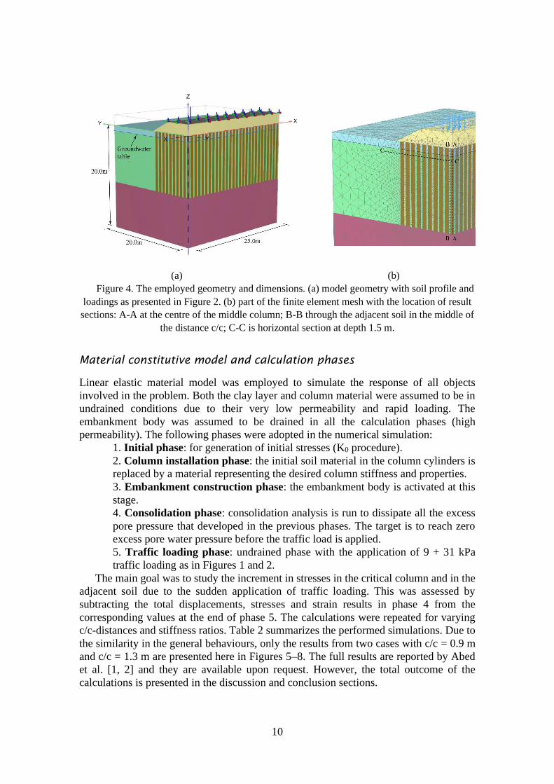
The 3D finite element calculations were performed using PLAXIS 3D [22]. Figure 4

illustrates the problem geometry, dimensions and finite element mesh (for more details

about the dimensions, see Figure 2). Due to symmetry, only a quarter of the problem is

modelled. The example shown in Figure 4 represents the case of c/c = 0.9 m. The finite

element mesh consists of about 630 000 ten-noded tetrahedron elements with four stress

integration (Gauss) points per element.

10

(a) (b)

Figure 4. The employed geometry and dimensions. (a) model geometry with soil profile and

loadings as presented in Figure 2. (b) part of the finite element mesh with the location of result

sections: A-A at the centre of the middle column; B-B through the adjacent soil in the middle of

the distance c/c; C-C is horizontal section at depth 1.5 m.

Material constitutive model and calculation phases

Linear elastic material model was employed to simulate the response of all objects

involved in the problem. Both the clay layer and column material were assumed to be in

undrained conditions due to their very low permeability and rapid loading. The

embankment body was assumed to be drained in all the calculation phases (high

permeability). The following phases were adopted in the numerical simulation:

1. Initial phase: for generation of initial stresses (K0 procedure).

2. Column installation phase: the initial soil material in the column cylinders is

replaced by a material representing the desired column stiffness and properties.

3. Embankment construction phase: the embankment body is activated at this

stage.

4. Consolidation phase: consolidation analysis is run to dissipate all the excess

pore pressure that developed in the previous phases. The target is to reach zero

excess pore water pressure before the traffic load is applied.

5. Traffic loading phase: undrained phase with the application of 9 + 31 kPa

traffic loading as in Figures 1 and 2.

The main goal was to study the increment in stresses in the critical column and in the

adjacent soil due to the sudden application of traffic loading. This was assessed by

subtracting the total displacements, stresses and strain results in phase 4 from the

corresponding values at the end of phase 5. The calculations were repeated for varying

c/c-distances and stiffness ratios. Table 2 summarizes the performed simulations. Due to

the similarity in the general behaviours, only the results from two cases with c/c = 0.9 m

and c/c = 1.3 m are presented here in Figures 5–8. The full results are reported by Abed

et al. [1, 2] and they are available upon request. However, the total outcome of the

calculations is presented in the discussion and conclusion sections.

11

Calculation results

Figure 5 presents the total displacements at the end of the calculations. This figure serves

as a reference for the general response of the numerical model and adequacy of the

position of the boundary conditions. It also shows that the model behaves qualitatively as

expected and that the problem boundaries were correctly decided and were far enough to

avoid any disturbance to the solution domain.

Figure 6 shows results along the section C-C at the depth of –1.5 m and Figure 7 along

sections A-A and B-B along the critical column and the adjacent soil. Respectively the

case of c/c = 0.9 m and stiffness ratio of Ecol / Esoil = 2.4 is presented in the a-figures and

the case of c/c = 1.3 m and stiffness ratio of Ecol / Esoil = 8.1 in the b-figures.

Figure 8 illustrates some characteristic output of the calculations. These results are for

the case of c/c = 1.3 m and stiffness ratio of Ecol / Esoil = 2.4.

Figure 5. Model response: total displacement at the end of analysis

12

Figure 6. Calculation results, vertical displacement increment and vertical stress increment

at the section C-C. Level 0 m is the bottom of the embankment. (a) c/c = 0.9 m + Ecol / Esoil = 2.4

and (b) c/c = 1.3 m + Ecol / Esoil = 8.1. Legends: total stress increment (zz), effective stress

increment (zz’) and excess pore pressure increment (pExcess).

13

Figure 7. Calculation results, effective stress increment in the z-direction, y-direction and

ratio between horizontal (y) and vertical (z) effective stress increments at sections A-A and B-B

along the critical column and the adjacent soil, respectively. Level 0 m is the bottom of the

embankment. (a) c/c = 0.9 m + Ecol / Esoil = 2.4. (b) c/c = 1.3 m + Ecol / Esoil = 8.1.

14

(a) (b)

Figure 8. Example of the typical calculation output: (a) total vertical stress before traffic

loading; and (b) excess pore water pressure after traffic loading (max ≈ 20kPa).

Discussion

Figure 9 illustrates the results of the eight calculations listed in Table 2. The vertical axis

shows the depth from the road surface and the horizontal axis the calculated averaged

vertical total stress increments due to traffic load. The numbers represent weighted values

(with respect to the area of c/c by c/c supported by one column) from each stress

increment carried by the column and by the soil. The averaged vertical total stress

increment due to traffic load is expressed by:

Δσzaverage=

Δσzcol×Acol+Δσzsoil

×Asoil

Acol + Asoil (14)

In Equation 14, Acol and Asoil are the horizontal cross-section areas of the column and

soil, respectively. The symbol Δσz,average stands for the average value of vertical stress

increment.

Figure 10 presents values of averaged vertical total stress increment due to traffic load

compared to the results calculated with the Boussinesq and 2:1 -stress distribution

theories. It appears that conclusive differences exist between the results from the

Boussinesq, the 2:1 stress distribution and the results from 3D FEM calculated values.

∆σz,average−∆σz,Boussinesq

Δσz,Boussinesq∙ 100 [%] (15)

∆σz,average−∆σz,2:1

Δσz,2:1∙ 100 [%] (16)

15

Figure 9. Average vertical stress increment for c/c = 0.9 m and 1.3 m with different moduli

ratios of Ecol / Esoil.

Figure 10. Average vertical stress increment and comparison to the Boussinesq and 2:1 -stress

distributions.

16

Table 3 presents the differences between FEM-calculated values and results from the

Boussinesq stress distribution (Eq. 15) and the 2:1 stress distribution (Eq. 16) methods at

the depths of 3, 4 and 5 meters from the road surface.

Table 3. Difference in the total stress increment due to traffic between 3D FEM calculated

results and values from the Boussinesq and the 2:1 stress distribution methods at the depths of 3,

4 and 5 meters from the road surface. All stress distributions are presented in Figure 10.

Depth

from road

surface

Difference between 3D FEM and

Boussinesq-calculated Δσz,average (Eq.

14)

Difference between 3D FEM and 2:1-

stress-distribution-calculated Δσz,average

(Eq. 15)

3 m +4 %...–28 % +25 %...–14 %

4 m +18 %...–16 % +27 %...–10 %

5 m +37 %...–6 % +33 %...–9 %

Design

Calculation results presented in Figure 9 are adopted in the new stabilisation design

guidebook by FTA [7]. Both the new guidebook [7] and the previous guidebook by FTA

[9] contain design examples. In one of these examples the geometry of the embankment

and the soil layers are similar to those in the case of FEM analyses portrayed in this paper

(Figure 2).

In stability calculations the change consists of an increase in the traffic load from the

previously used 10 kPa to 12 kPa, developed for standard cases from the traffic load in

NCCI7 [8]. The settlement calculations and the verifying of arching on columns are

identical in both the FTA 2010 and 2018 guidelines. The main adjustments are in the

traffic loading and in verifying the compression capacity of the top of the columns.

The design example of FTA with the traffic load of 10 kPa (Appendix 2 in [9]) gives

as a result the column ratio of a = 0.35 (a = Acol / ( Asoil + Acol ) ) with the shear strength

of 100 kPa for columns. The same example with the new traffic load (Appendix 3 in [7])

gives also result of a = 0.35. When the shear strength of the columns is 100 kPa, this

results in columns with the diameter of 600 mm having a column distance of c/c = 0.90

m or with the diameter of 700 mm having a column distance of 1.05 m. This means that

the number of columns ends up as the same in the two cases – both with the previous

traffic load of 10 kPa and with the new one of 9 + 31 kPa, where 31 kPa impacts an area

of 3 m x 5 m. Obviously this design example is not a universal result and for instance

when no dry crust exists under a moderately thin embankment, the new traffic load leads

to either a smaller c/c-distance, a larger column diameter or higher column strength.

Similarly, the increase in the Ecol to Esoil ratio results in a smaller c/c-distance, a larger

diameter or higher strength of the columns.

Conclusions

Due to Eurocode recommendations there have been major increase in the intensity of the

traffic loading. The 3D simulations were done to better understand the interaction

17

between column and soil under a rapid traffic load. The results proved that the average

vertical stress increment decreases downwards as expected, but the magnitude of the

decrease differs significantly from the one determined with either the Boussinesq or the

2:1 stress distribution theory. The vertical stress increment increases when the distance

between columns decreases (from 1.3 m to 0.9 m) or when the ratio between the column

and soil stiffness increases.

The aforementioned results were implemented into the updated design guidelines of

Finnish Transport Agency [7] in the analytical dimensioning of deep stabilisation. On the

basis of some design examples it appears that the previous design method with the traffic

load of 10 kPa leads to quite the similar number of columns as with the new traffic load

of 9 + 31 kPa regardless of the theoretical inadequacy in the previous traffic load

consideration. If no dry crust exists under a moderately thin embankment, the new traffic

loading and dimensioning leads to more conservative design with smaller c/c distance,

larger columns or higher column strength.

Acknowledgements

The authors would like to acknowledge the Finnish Transport Agency, Ramboll Finland

Oy and Aalto University, which collectively funded this 3D modelling project.

References

[1] A. Abed, L. Korkiala-Tanttu, J. Forsman. 3D Stress distribution modelling of deep

mixing columns (Part II). Aalto University, Helsinki. 15 p, 2018.

http://dx.doi.org/10.13140/RG.2.2.35120.38400

[2] A. Abed, L. Korkiala-Tanttu, J. Forsman. 3D Stress distribution modelling of deep

mixing columns. Aalto University, Helsinki. 7 p, 2017.

http://dx.doi.org/10.13140/RG.2.2.31764.94084

[3] B. Broms, P. Boman. Stabilisation of soil with lime columns. Design Handbook.

92. Royal Institute of Technology, Department of Soil and Rock Mechanics,

Sweden. 92 p, 1977.

[4] C. Chan. A laboratory investigation of shear wave velocity in stabilised soft soils.

PhD Thesis. University of Sheffield. UK. 234 p, 2006. Available at:

http://etheses.whiterose.ac.uk/15165/1/425591.pdf (Accessed: 17 July 2020).

[5] M. Dahlström. Dry soil mixing. In: Moseley, M. & Kirsch, K (Eds.). Ground

Improvement. Second Edition, Taylor & Francis. New York. ISBN-13: 978-

0415274555, pp. 435–494, 2012.

[6] Finnish Road Administration, FINNRA. Teiden pohjarakenteiden

suunnitteluperusteet “Design criteria for road base structures”, TIEH 2100002-

01. Finland. In Finnish. ISBN 951-726-743-6, 60 p, 2001.

[7] Finnish Transport Agency. Syvästabiloinnin suunnittelu “Deep stabilization

planning” (in Finnish) Liikenneviraston ohjeita 17/2018. Liikennevirasto,

Helsinki. ISBN 978-952-317-588-4, 128 p, 2018.

[8] Finnish Transport Agency. Eurokoodin soveltamisohje Geotekninen suunnittelu –

NCCI 7 “NCCI7 Geotechnical Design, Application guidelines for Eurocode in

18

Finnish FTA’s guideline” 13/2017 21.4.2017 (in Finnish). Helsinki. SBN 978-952-

317-387-3. 91 p, 2017.

[9] Finnish Transport Agency. Syvästabiloinnin suunnittelu “Deep stabilization

planning” (in Finnish) Liikenneviraston ohjeita 11/2010. Liikennevirasto,

Helsinki. ISBN 978-952-255-030-9, 57 p, 2010.

[10] J. Forsman, L. Korkiala-Tanttu, P. Piispanen. Mass Stabilisation as a Ground

Improvement Method for Soft Peaty Soil. In: Topcuoglu, B. & Turan, M. Peat.

InTechOpen. pp. 107–139, 2018. http://dx.doi.org/10.5772/intechopen.74144

[11] M. Hassan. Engineering characteristics of cement stabilised soft Finnish clay - a

Laboratory study, Licentiate thesis, Helsinki University of Technology, Espoo, 72

p, 2009.

[12] K. Koivisto. Katuliikenteen aiheuttaman tärinän vähentäminen syvästabiloinnin

avulla “Use of Deep Stabilisation as a Countermeasure against Vehicle Generated

Ground Vibration”. MSc thesis. in Finnish. Helsinki University of Technology.

120 p, 2004.

[13] K. Koivisto, J. Hellberg, J. Forsman. "Finite Element Modelling of Deep

Stabilisation Test Structures Used in Attenuating Railway Induced Ground

Vibration at Koria, Finland" in M. Kitazume, M. Terashi, S. Tokunaga & N.

Yasuoka (eds.) Deep Mixing 2009 Okinawa Symposium, Proceedings of The

International Symposium on Deep Mixing & Admixture Stabilisation –

DM'09/Okinawa, Japan/19–21 May 2009. Sanwa Co., Ltd. pp. 471–476, 2009.

[14] K. Koivisto, J. Hellberg, J. Forsman. "LITES 2 – Eliminating traffic induced

vibrations by means of deep stabilisation, phase 2. Report 1 B: Computational

Analysis of the Alternative Structures", unpublished report. By Ramboll Finland

Oy to Finnish Rail Administration, 2008.

[15] P. Kolisoja. Sitomattomien kerrosten kiviainesten muodonmuutosominaisuudet:

esiselvitysvaiheen kuormituskokeet “Deformation properties of aggragetes of

unbound layers. Loading tests of preliminary test series”. Tielaitoksen selvityksiä

39/1993. in Finnish. Tielaitos. Helsinki. ISBN 951-47-7670-4, 71 p, 1993.

[16] S. Köylijärvi. Saven anisotropian ja destrukturaation vaikutuksen mallintaminen

Östersundomin koepenkereellä “Effect of anisotropy and destructuration on the

behaviour of Östersundom test embankment”, Master's Thesis Aalto University.

(in Finnish). 96 p, 2015.

[17] F. Kulhawy, P. Mayne. Manual on estimating soil properties for foundation

design. Electric Power Research Inst., Palo Alto, CA (USA); Cornell Univ., Ithaca,

NY (USA). Geotechnical Engineering Group. 241 p, 1990. Available at:

https://www.geoengineer.org/storage/publication/20489/publication_file/2745/EL-

6800.pdf (Accessed: 17 July 2020).

[18] R. Larsson, M. Mulabdic’. Shear moduli in Scandinavian clays. Shear moduli in

Scandinavian clays: measurements of initial shear modulus with seismic cones:

empirical correlations for the initial shear modulus in clay. Swedish Geotechnical

Institute. 40. ISSN 0348-0755, 127 p, 1991. Available at: https://www.diva-

portal.org/smash/get/diva2:1299970/FULLTEXT01.pdf (Accessed: 17 July 2020).

[19] M. Löfman. Perniön saven parametrien luotettavuuden ja saven eri

ominaisuuksien välisten korrelaatioiden arviointi “Estimation of the reliability of

19

Perniö clay parameters and correlations between clay properties”, Master's thesis

Aalto University. In Finnish. 121 p, 2016.

[20] J. Mäenpää. Seismisen CPTU-mittauksen käyttö leikkausaallon nopeuden

määrittämiseen “Determining shear wave velocity by seismic CPTU”. Master's

thesis, Technical University of Tampere. In Finnish. 96 p, 2016.

[21] M. Navin. Stability of embankments founded on soft soil improved with deep-

mixing-method columns. PhD Thesis. Virginia Polytechnical Institute. 188 p,

2005. Available at:

https://vtechworks.lib.vt.edu/bitstream/handle/10919/28654/dissertation_revised.p

df?sequence=2&isAllowed=y (Accessed: 17 July 2020).

[22] PLAXIS 3D. Plaxis bv. Delft. The Netherlands, 2016.

[23] H. Poulos, E. Davis. Elastic solutions for soil and rock mechanics. John Wiley &

Sons. New York. 411 p, 1974.

[24] B. Ringesten. Dry crust - its formation and geotechnical properties. PhD thesis.

Chalmers University of Technology. Göteborg. Sweden. ISSN 0346-718X, 191 p,

1990.

[25] N. Ronkainen. Suomen maalajien ominaisuuksia Suomen Ympäristö

“Characteristics of Finnish soils” 2/2012. In Finnish. ISBN 978-952-11-3975-8.

62 p., 2012.

[26] P. Robertson. Seismic CPT (SCPT) [PowerPoint presentation]. Second

International Conference on Deep Foundations (2C.F.P.B): Field Testing and

Construction Aspects of Deep Foundations. Campo Ferial Fexpocruz, Santa Cruz,

Bolivia, 12–15 May, 2015. Available at:

http://cfpbolivia.com/2015/Robertson/Seismic-cpt(scpt)-peter-robertson.pdf

(Accessed: 28 February 2019).

[27] Swedish Road Administration (Trafikverket). Trafikverkets tekniska krav för

geokonstruktioner TK Geo13 (No. TRV 2014/13914). Swedish Road

Administration, Sweden. In Swedish. 105 p, 2014. Available at:

http://www.th.tkgbg.se/Portals/0/STARTFLIKEN/Checklistor%20och%20mallar/2

_%20Projektering%20dokument/TK%20Geo%2013%20Trafikverkets%20teknisk

a%20krav%20f%C3%B6r%20geokonstruktioner_2015-12.pdf (Accessed: 28

February 2019).

[28] M. Timoney. Strength verification methods for stabilised soil-cement columns: a

laboratory investigation of PORT and PIRT. PhD Thesis. National University of

Ireland, Gal-way. 328 p, 2015. Available at:

https://aran.library.nuigalway.ie/handle/10379/5023 (Accessed: 17 July 2020).

[29] J. Toikka, P. Virtala. Axle weight study 2013–2014. Research reports of the Finnish

Transport Agency 67/2015. Finnish Transport Agency, Helsinki. ISBN 978-952-

317-179-4, 74 p, 2015.

[30] M. Topolnicki. In-situ soil mixing. In: M. Moseley, K. Kirsch (Eds.) Ground

Improvement. Second Edition, CRC Press. 488 p, 2004.

[31] J. Vinter. The effect of the sub-ballast layer material to the performance of ground-

supported railway embankment. Master's thesis. In Finnish. Aalto University

Espoo. 96 p, 2015.

[32] U. Vogler. Numerical modelling of deep mixing with volume averaging technique.

PhD Thesis. The University of Strathclyde. Strathclyde. UK. 233 p, 2008.

20

[33] C. Wroth. In-situ measurements on initial stresses and deformations characteristics.

Proceedings Conference in-situ Measurements of Soil Properties. Raleigh. North

Carolina. Vol. 2, pp. 181–230, 1975.

Ayman A. Abed

Chalmers University of Technology

Department of Architecture and Civil Engineering

Sweden

Formerly:

Aalto University

Department of Civil Engineering

P.O.Box 12100, FI-00076 Aalto

Finland

ayman.abed@chalmers.se

Leena Korkiala-Tanttu

Aalto University

Department of Civil Engineering

P.O.Box 12100, FI-00076 Aalto

Finland

leena.korkiala-tanttu@aalto.fi

Juha Forsman, Kirsi Koivisto

Ramboll Finland Oy

Espoo

Finland

juha.forsman@ramboll.fi, kirsi.koivisto@ramboll.fi