ABC-Miner+: Constructing Markov Blanket Classi ers … · (will be inserted by the editor)...
40
Memetic Computing manuscript No. (will be inserted by the editor) ABC-Miner+: Constructing Markov Blanket Classifiers with Ant Colony Algorithms Khalid M. Salama · Alex A. Freitas 15-09-2013 Abstract ABC-Miner is a Bayesian classification algorithm based on the Ant Colony Optimization (ACO) meta-heuristic. The algorithm learns Bayesian network Augmented Na¨ ıve-Bayes (BAN) classifiers, where the class node is the parent of all the nodes representing the input variables. However, this as- sumes the existence of a dependency relationship between the class variable and all the input variables, and this relationship is always a type of “causal” (rather than “effect”) relationship, which restricts the flexibility of the algo- rithm to learn. In this paper, we extended the ABC-Miner algorithm to be able to learn the Markov blanket of the class variable. Such a produced model has a more flexible Bayesian network classifier structure, where it is not nec- essary to have a (direct) dependency relationship between the class variable and each of the input variables, and the dependency between the class and the input variables varies from “causal” to “effect” relationships. In this context, we propose two algorithms: ABC-Miner+ 1 , in which the dependency relation- ships between the class and the input variables are defined in a separate phase before the dependency relationships among the input variables are defined, and ABC-Miner+ 2 , in which the two types of dependency relationships in the Markov blanket classifier are discovered in a single integrated process. Em- pirical evaluations on 33 UCI benchmark datasets show that our extended algorithms outperform the original version in terms of predictive accuracy, model size and computational time. Moreover, they have shown a very com- petitive performance against other well-known classification algorithms in the literature. Keywords: Ant Colony Optimization (ACO), Data Mining, Classification, Bayesian Networks, Markov Blanket Classifiers . School of Computing, University of Kent, Canterbury, CT2 7NF, UK E-mail: {kms39,A.A.Freitas}@kent.ac.uk
-
Upload
nguyenhuong -
Category
Documents
-
view
216 -
download
0
Transcript of ABC-Miner+: Constructing Markov Blanket Classi ers … · (will be inserted by the editor)...

Memetic Computing manuscript No.(will be inserted by the editor)
ABC-Miner+: Constructing Markov Blanket Classifierswith Ant Colony Algorithms
Khalid M. Salama · Alex A. Freitas
15-09-2013
Abstract ABC-Miner is a Bayesian classification algorithm based on the AntColony Optimization (ACO) meta-heuristic. The algorithm learns Bayesiannetwork Augmented Naıve-Bayes (BAN) classifiers, where the class node isthe parent of all the nodes representing the input variables. However, this as-sumes the existence of a dependency relationship between the class variableand all the input variables, and this relationship is always a type of “causal”(rather than “effect”) relationship, which restricts the flexibility of the algo-rithm to learn. In this paper, we extended the ABC-Miner algorithm to beable to learn the Markov blanket of the class variable. Such a produced modelhas a more flexible Bayesian network classifier structure, where it is not nec-essary to have a (direct) dependency relationship between the class variableand each of the input variables, and the dependency between the class and theinput variables varies from “causal” to “effect” relationships. In this context,we propose two algorithms: ABC-Miner+1, in which the dependency relation-ships between the class and the input variables are defined in a separate phasebefore the dependency relationships among the input variables are defined,and ABC-Miner+2, in which the two types of dependency relationships in theMarkov blanket classifier are discovered in a single integrated process. Em-pirical evaluations on 33 UCI benchmark datasets show that our extendedalgorithms outperform the original version in terms of predictive accuracy,model size and computational time. Moreover, they have shown a very com-petitive performance against other well-known classification algorithms in theliterature.
Keywords: Ant Colony Optimization (ACO), Data Mining, Classification,Bayesian Networks, Markov Blanket Classifiers .
School of Computing, University of Kent,Canterbury, CT2 7NF, UKE-mail: {kms39,A.A.Freitas}@kent.ac.uk

2 Khalid M. Salama, Alex A. Freitas
1 Introduction
Ant Colony Optimization (ACO) is a meta-heuristic for solving combinatorialoptimization problems, inspired by the observation of the behavior of biolog-ical ant colonies [14]. One of the fields in which ACO has been successfullyapplied is data mining, which involves finding hidden patterns and construct-ing analytical models from real-world datasets [53]. Classification is one of thewidely studied data mining tasks, where the aim is to discover, from labeledcases (instances), a model that can be used to predict the class of unlabeledcases. There are many types of classification methods [53], but in this paperwe focus on Bayesian network (BN) classifiers.
BN classifiers model the (in)dependency-relationships between the inputdomain variables given the class variable by means of a probabilistic network[18], which is used to predict the class of a case by computing the class with thehighest posterior probability given the case’s predictor attribute values. Sincelearning the optimal BN structure from a dataset is NP-hard [5,6], stochasticheuristic search algorithms – such as ACO – can be a good alternative to buildhigh-quality models, in terms of predictive accuracy and network size, withinan acceptable computational time. Developing ACO-based algorithms to learnBN classifiers is the research topic addressed in this work.
We have recently introduced ABC-Miner [45,49], as an Ant-based BayesianClassification algorithm that learns the structure of a Bayesian network Aug-mented Naıve-Bayes (BAN), where the class node is the parent of all the inputvariables, and at most k parents are allowed for each variable in the network.The ABC-Miner algorithm showed predictive effectiveness compared to otherBayesian classification algorithms, namely: Naıve-Bayes, TAN and GBN [45,49]. However, the BAN structure produced by ABC-Miner has two limitations.First, it assumes there is a dependency relationship between the class and allthe input variables. However, this assumption is unrealistic and may harm theclassification effectiveness in the domains where there are redundant or irrele-vant input variables to the class variable prediction. Second, this dependencyrelationship between the class and the input variables is only specified as a“causal” relationship, i.e., the class variable is always a parent to the inputvariables. This restricts the flexibility of the algorithm to discover other struc-tures in constructing BN classification models, where the relationship betweenthe class and an input variable is an“ effect” relationship — i.e., the classvariable can be a child to some input variables.
In this paper, we extend our ABC-Miner algorithm to learn more flexibleBN classifier structures, where it is not necessary to have a (direct) depen-dency relationship between the class variable and each of the input variables.In addition, we allow the dependency between the class and the input vari-ables to vary from “causal” to “effect” relationships, where the class variablecan be a parent or a child of an input node. The produced model is calledthe Markov blanket (MB) of the class variable. Such a model specifies a moreeffective posterior probability distribution of the class variable given the sub-set of input variables that are relevant to the class prediction, which avoids

Title Suppressed Due to Excessive Length 3
the negative effect of the redundant and irrelevant input variables to the tar-get class. In this context we propose two variations of ACO-based algorithmsfor learning Markov blanket classifiers. The first algorithm is ABC-Miner+1,which executes in two phases. The first phase is dedicated to construct a struc-ture where only the relationship types (if any exists) between the class andthe input variables are defined, while in the second phase the dependency re-lationships among the input variables, according to the previously discoveredstructure, are defined. The second algorithm, ABC-Miner+2, utilizes an inte-grated approach, where the whole MB structure – including the dependencyrelationships between the class and the input variables, and among the inputvariables – is constructed in a synergic fashion.
The present paper is an extended version of the NICSO 2013 workshoppaper [48], where ABC-Miner+1, the two-phase ACO algorithm for learningMB classifiers, was introduced. We build on the work described in [48] in fourways. First, we introduce the novel ABC-Miner+2 algorithm, which discoversthe dependency structure of the MB classifier in a single integrated phase.Second, in order to mitigate possible training-phase overfitting, we propose twonew ideas: 1) randomly changing the validation set during the training phaseat each iteration; and 2) introducing a new penalty component in the modelquality evaluation function according to the number of class variable parents tolimit it and avoid producing overfitted structures. Third, we use two differenttypes of classification measures to evaluate the quality of the candidate modelconstructed during the training phase: accuracy and probabilistic accuracy.Fourth, in terms of empirical evaluations, the number of datasets used inthe experimental evaluation is increased from 18 to 33, and we compare ourproposed algorithms with various well-known classification algorithms.
Note that we use the word “causal” in a loose sense in this work, simply torefer to a direction of the dependency relationship between two variables. Theissue of whether or not Bayesian networks learned from observational datarepresent truly causal knowledge is controversial (depending on how we definecausality) [41], and is out of the scope of this paper.
The rest of the paper is structured as follows. The next section gives somebackground on the two related areas of this research, namely BN classifiersand ACO. Then, we briefly review the ABC-Miner algorithm in Section 3,to make this paper more self-contained. In Section 4, we discuss the motiva-tion behind our target task, which is learning Markov blanket classifiers, andthe difference between directly aiming at that target and learning GeneralBayesian Networks (GBNs) and then extracting the class variable’s MarkovBlanket. We introduced our two ACO-based algorithms, ABC-Miner+1 andABC-Miner+2, in Section 5, along with the quality evaluation functions usedin our algorithms for building the MB classification models and the overfittingmitigation techniques. Our experimental methodology is presented in Section6, followed by the computational results and their analysis in Section 7. Finally,we conclude with general remarks in Section 8.
4 Khalid M. Salama, Alex A. Freitas
2 Background
2.1 Bayesian Networks
Bayesian Networks (BNs) are a statistically sound method for representingprobabilistic (in)dependencies among variables and using those (in)dependenciesfor probabilistic inferences [9]. In a BN, nodes represent variables (featuresor attributes) and edges represent dependencies among variables. The set ofnodes and edges forms a DAG (Directed Acyclic Graph). Each node in thatDAG is also associated with a Conditional Probability Table (CPT), whichspecifies the probability for each value of its variable given the values of allthe variables that are parents of that node. The set of CPTs are the set ofparameters Θ of the BN. The joint probability distribution of the set of vari-ables X = {X1, X2, X3, ..., Xn} in a BN given its DAG structure G and its setof parameters Θ is given by the following factorized formula:
P (X1, X2, ..., Xn) =n∏
i=1
P (Xi|Parents(Xi), Θ,G), (1)
where Parents(Xi) are the parents of variable Xi, and G is the DAG thatrepresents the BN’s structure.
Learning a BN from a dataset involves two steps: learning the DAG struc-ture, and then learning the set of parameters Θ. The DAG structure learningstep is usually considered the most difficult one, since parameter learning canbe performed by estimating the relative frequency of each variable value di-rectly from the dataset.
Broadly speaking, there are two approaches for learning the DAG structureof a BN. The first one is often called the CI-based (Conditional Independence-based, or constraint-based) approach [23,9]. This approach is based on itera-tively using some kind of statistical independence test (e.g. the Chi-squaredtest) to detect whether a certain set of variables is (in)dependent – possiblygiven other variables. Two issues with this approach are that the results of suchstatistical tests are quite sensitive to the value of a (ad-hoc) user-specified sig-nificance level value and the iterative use of such tests leads to the well-knownproblem of multiple statistical hypothesis testing.
By contrast, the second approach, usually called the scoring-based ap-proach, uses a scoring function to evaluate each DAG structure G with respectto the dataset D at hand [23,9]. The basic idea is to find the DAG structureG that best fits the dataset D in terms of P (D|G). This idea is implementedby using a search method (usually a greedy one) G that maximizes the valueof a given scoring function. This approach has been more popular in the datamining and machine learning fields, possibly because it views the problem ofBN learning as a well-defined optimization task (avoiding difficult issues ofmultiple hypothesis testing), where various types of search methods can beemployed [4]. K2, MDL, KL, BDEu and several scoring functions can be usedfor this scoring-maximization task [7,24,55].

Title Suppressed Due to Excessive Length 5
For a more detailed review on learning BNs, we recommend the very com-prehensive review by Daly et al. [9] as well as [24,23].
2.2 Bayesian Network Classifiers
A general-purpose BN can compute the probability of any set of variables’values given any other set of variables’ values. By contrast, a BN classifieris built specifically for the classification task, i.e., to compute the probabilityof each value of the class variable for an instance given the values of all theother variables of that instance. More formally, a BN classifier computes theposterior probability of each value (label) l of the class variable C given aninstance x = (x1, x2, ..., xn) using a DAG structure G and parameters Θ, thenlabels this case with the class value having the highest posterior probability,as show in the following formulas:
C(x) = argmax∀ l∈C
P (C = l|x = x1, x2, ..., xn, BNC), (2)
and according to the Bayes’ theorem,
posterior probability︷ ︸︸ ︷P (C = l|x = x1, x2, ..., xn) ∝
prior probability︷ ︸︸ ︷P (C = l)
n∏i=1
likelihood︷ ︸︸ ︷P (xi|Parents(Xi)) , (3)
where ∝ denotes the proportionality relationship. The above formulas referto a typical type of BN classifier, where the class variable is a parent (cause)node to all the input variables (predictor attributes). As will be seen later,this is not the case in all types of BN classifiers.
Among the many types of BN classifiers, the simplest one is Naıve-Bayes(NB) [15,18]. NB makes the assumption that the input variables are inde-pendent of each other given the class variable, so its network has no edgesconnecting input variables. This reduces the posterior probability formula to:
P (C = l|x = x1, x2, ..., xn) ∝ P (C = l)
n∏i=1
P (xi|l) (4)
Since the assumption of independence among input variables is usuallynot realistic, many extensions of NB have been proposed. As discussed in[28,56], those extensions can be broadly divided into three main approaches:1) applying NB to a subset of the input variables [31,34,27]; 2) extendingthe network structure of NB [3,4,19]; and 3) building local models based ondifferent subsets of the dataset [25,21,33,4,30,50]. The current work is relatedto the first two types of extensions.
The first approach, called feature selection [31,35], consists of selecting asubset of relevant variables (features) from the dataset for use in model con-struction. This is in contrast to conventional NB, where all the input variableshave some effect on computing the posterior probability of the class, and so
6 Khalid M. Salama, Alex A. Freitas
redundant, strongly-correlated, and irrelevant variables may degrade the pre-dictive performance of NB. Several feature selection methods were introducedin the literature, such as Backward Sequential Elimination (BSE) method [31],Forward Sequential Selection (FSS) [34], and Evolutional Naıve-Bayes (ENB)[27].
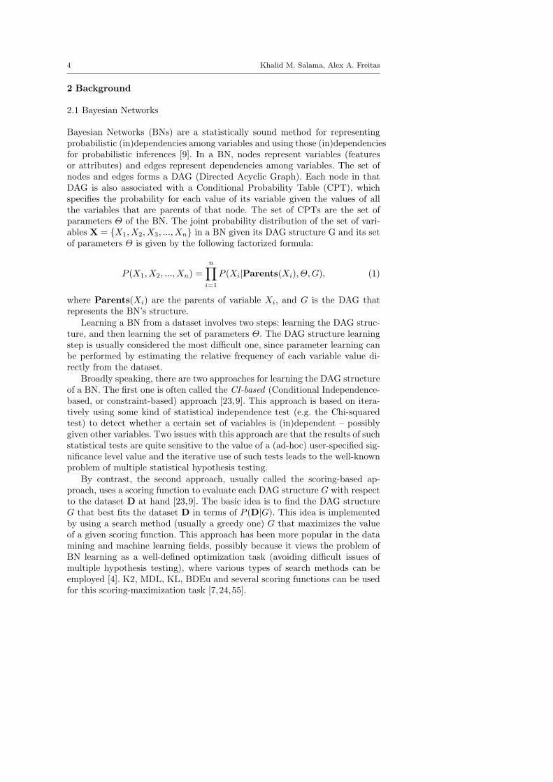
The second approach to improve NB is extending its structure to representthe dependency relationships between the input variables given the class vari-able, adding edges edges between the input nodes in the network. In practice,imposing restrictions on the number of parents that an input node can have inthe BN classifier is important for at least two reasons. First, finding the opti-mal structure of a BN (classifier) is NP-hard [5,6], thus restricting the numberof dependencies would reduce the search space and make the problem com-putationally tractable. Second, including too many dependency relationshipsin the BN classifier may result in producing a complex classification modelthat is prone to overfitting the training set and does not generalize well onthe test set. Besides, BN models with a large number of edges tend to be lesscomprehensible and harder to be interpreted by the user. Figure 1 illustratesthe various structural types of BN classifiers.
Fig. 1 Different types of Bayesian classifiers are presented: (a) Naıve-Bayes, where all theinput variables have only the class variable as a parent. (b) TAN, where a variable can haveone parent besides the class variable. (c) BAN, where a variable can have multiple parentsbeside the class variable. (d) MBC, where the class variable can have both parent and childvariables.
A simple extension of NB is the Tree Augmented Naıve-Bayes (TAN),which allows a node in a BN to have one parent, in addition to the class variable[18]. This produces a BN with a tree-like structure. The Chow-Liu tree (CL-Tree) [3,4], and the SuperParent TAN (SP-TAN) algorithms are examples ofwell-known TAN classifier learning algorithms. A more elaborated extension
Title Suppressed Due to Excessive Length 7
of NB is the Bayesian Network Augmented Naıve-Bayes (BAN). In a BAN,either there are no restrictions on the number of parents of a node or, morecommonly, there is a maximum number of k parents (k-dependencies) that anode can have. Another variation of the Chow-Liu algorithm can be utilizedto build BANs as well [3,4]. Note that if k = 1 a BAN becomes a TAN. Theoriginal version of our ABC-Miner algorithm produces BN classifiers with aBAN structure [49]. Since, the Markov blanket classifier (MBC), Figure 1 (d),is the focus of the current work; it is discussed separately in Section 4.
2.3 Ant Colony Optimization
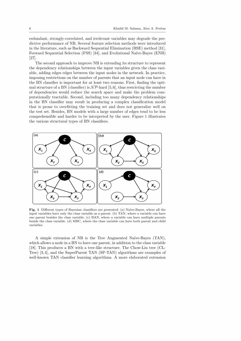
Ant colony optimization (ACO) is a meta-heuristic inspired by the behaviorof natural ant colonies [14,13,12]. Although each individual ant has a simplebehavior, the ants in a colony cooperate with each other to solve complexoptimization problems, resulting in an emergent intelligent behavior at thelevel of the colony. The pseudo-code of a typical ACO algorithm is shown, ata high level of abstraction, in Algorithm 1.
Algorithm 1 Pseudo-code of basic ACO algorithm.Begin ACOConstructionGraph← Problem definition;Initialize();best← ϕ; /* best solution found so far */repeat
current← ant.ConstructSolution()ApplyLocalSearch(current)if Quality(current) > Quality(best) then
best← current;end ifant.UpdatePheromone(current);
until termination condition
return best;End
The first step of Algorithm 1 is the definition of the construction graph,whose nodes represent the components to be used to construct a candidatesolution to the target problem. In the repeat-until loop, first each ant incre-mentally constructs a candidate solution by following a path in the graph,choosing which components are added to the current candidate solution ina heuristic manner (see below). Then, a local search procedure is applied tothe just-constructed candidate solution, in order to try to improve it. Next,the quality of the current candidate solution is evaluated, and the quality ofthe best solution constructed so far by the algorithm is tracked and saved inthe “best” variable. In the last step of the repeat-until loop, the current antdeposits pheromone on the construction graph components that were includedin its constructed candidate solution.

8 Khalid M. Salama, Alex A. Freitas
Importantly, the amount of pheromone deposited on each graph compo-nent is proportional to the quality of the current candidate solution, whichis measured by a predefined quality evaluation function. In future iterations,ants will be attracted by larger amounts of pheromone. Hence, the depositof pheromone acts as a positive feedback mechanism, which encourages theants to prefer solution components that were often used to produce good solu-tions in the previous iterations of the search. The algorithm also incorporatesa pheromone evaporation strategy (not shown in the high-level pseudo-codeof Algorithm 1), where the amount of pheromone in each solution componentdecreases gradually over time. This makes the search to put more emphasis onthe quality of solutions constructed in recent iterations, rather than in earlyiterations, helping convergence to good solutions.
In order to design an ACO algorithm, one has to specify not only a con-struction graph (representing solution components) and a quality-evaluationfunction, but also the state transition formula used by each ant to decide whichcomponent should be added next to the current solution. A typical state tran-sition formula consists of the product of two factors: the heuristic value η andthe pheromone amount τ associated with each candidate solution component.The value of η is usually computed by a predefined “local” heuristic functionthat measures the quality of a solution component by itself, regardless of thequality of the entire solution using that component, and regardless of the pre-vious history of the search. By contrast, the value of τ is given by the amountof pheromone accumulated on a solution component, taking into account thehistory of the search – i.e., solution components that were used to build bettersolution in the past accumulate more pheromone, as mentioned earlier. Typ-ically, an ant chooses which component to add next to a candidate solutionwith a probability proportional to the product of the heuristic value η and thepheromone amount τ for that component. In addition, one also has to specifyspecific formulas for pheromone updating (based on the quality function) andpheromone evaporation, of course. All these design decisions will be specifiedin the context of our proposed ACO algorithm in later sections.
It is important to note that, unlike the conventional local, greedy searchmethods which are commonly used in search and optimization problems, anACO algorithm performs a global search for near-optimal solutions in thesearch space. The global search stems from using a population of ants whichis initially spread across different regions of the search space and which iter-atively cooperate with each other (based on the positive feedback associatedwith depositing more pheromone on better solution components) in order toconverge to a near-optimal solution.
ACO has been effectively used for learning general-purpose BNs [54,10,8,42], as well as different types of classification models [40,43,37,39,44,51].Moreover, ABC-Miner, recently introduced by the authors [45,49], is the firstACO algorithm for learning BN classifiers with a BAN structure, and it wasshown to outperform several BN classification algorithms. Thus, we extend theant-based ABC-Miner algorithm to learn the more advanced structure of MBclassifiers. The authors have also introduced a clustering-based Bayesian multi-
Title Suppressed Due to Excessive Length 9
net classification algorithm [47], which uses ACO to cluster the dataset intosubsets, then builds several local BN classifiers. However, this paper addressesthe problem of building BN classifiers with a very different approach.
3 An Overview of the ABC-Miner Algorithm
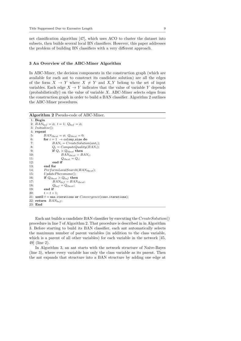
In ABC-Miner, the decision components in the construction graph (which areavailable for each ant to construct its candidate solution) are all the edgesof the form X → Y where X = Y and X,Y belong to the set of inputvariables. Each edge X → Y indicates that the value of variable Y depends(probabilistically) on the value of variable X. ABC-Miner selects edges fromthe construction graph in order to build a BAN classifier. Algorithm 2 outlinesthe ABC-Miner procedures.
Algorithm 2 Pseudo-code of ABC-Miner.1: Begin2: BANbsf = ϕ; t = 1; Qbsf = ϕ;3: Initialize();4: repeat5: BANtbest = ϕ; Qtbest = 0;6: for i = 1 → colony size do7: BANi = CreateSolution(anti);8: Qi = ComputeQuality(BANi);9: if Qi > Qtbest then10: BANtbest = BANi;11: Qtbest = Qi;12: end if13: end for14: PerformLocalSearch(BANtbest);15: UpdatePheromone();16: if Qtbest > Qbsf then17: BANbsf = BANtbest;18: Qbsf = Qtbest;19: end if20: t = t+ 1;21: until t = max iterations or Convergence(conv iterations);22: return BANbsf ;23: End
Each ant builds a candidate BAN classifier by executing the CreateSolution()procedure in line 7 of Algorithm 2. That procedure is described in in Algorithm3. Before starting to build its BAN classifier, each ant automatically selectsthe maximum number of parent variables (in addition to the class variable,which is a parent of all other variables) for each variable in the network [45,49] (line 2).
In Algorithm 3, an ant starts with the network structure of Naıve-Bayes(line 3), where every variable has only the class variable as its parent. Thenthe ant expands that structure into a BAN structure by adding one edge at

10 Khalid M. Salama, Alex A. Freitas
Algorithm 3 Pseudo-code of solution creation procedure by an ant.1: Begin CreateSolution(ant)2: k list = ant.SelectMaxParentsForEachV ariable();3: BAN ← Naıve-Bayes structure;4: while GetV alidEdges() = ϕ do5: {i→ j} = ant.SelectEdgeProbablistically();6: BAN = BAN ∪ {i→ j};7: RemoveInvalidEdges(BAN, kj);8: end while9: BAN.LearnParameters();10: return BAN ;11: End
a time to the network (lines 4 to 8). The edge selected to be added in thecurrent step is determined probabilistically. More precisely, the probability ofeach edge being selected is given by the product of the pheromone amount inthe edge (reflecting the usefulness of that edge for constructing good BANs inprevious iterations of the search) times the heuristic function value of that edge– measured by its conditional mutual information [45,49] (line 5). However, anedge can be added to the current BAN structure only if its inclusion does notproduce a directed cycle and does not violate the constraint on the maximumnumber of parents k (chosen by the current ant) for the node that the edge ispointing to. When an edge is added to the current BAN, all invalid edges areremoved from the construction graph (line 7). An ant keeps adding edges tothe current BAN as long as there are valid edges in the construction graph.Then, the CPT of each variable is computed, in order to create a completeBAN classifier (line 9). That classifier is then evaluated, and all edges becomeavailable again for constructing other BAN classifiers (line 8 in Algorithm 2).
ABC-Miner evaluates the quality of a candidate BAN classifier using ameasure of predictive accuracy [45,49], since the BAN will be used only forpredicting the value of a specific class attribute. This is in contrast to general-purpose BN learning algorithms, whose solution-quality function does not dis-tinguish between the input (predictor) and the class attributes. As shown inAlgorithm 2, only the colony’s iteration best solution BANtbest undergoes localsearch and is used for updating pheromone (lines 14 and 15). The best-so-farsolution BANbsf is saved during the search and returned as the output of thealgorithm.
4 Learning Markov Blanket Classifiers
4.1 Target and Motivation
The motivation behind our proposed extension is the following. As discussed inSection 2.2, two different limitations can be concluded from conventional TANand BAN, which are the commonly used structures of the BN classifier thatextends Naıve-Bayes. First, it assumes that the class variable has dependency

Title Suppressed Due to Excessive Length 11
relationships with all the input variables (attributes), which means that thestate of each input variable affects the posterior probability of the class values,and consequently the class prediction. This assumption is not necessarily validin all applications domains. In some domains, some attributes are irrelevant,or at least not directly related, to the prediction of the target class. Includingthese irrelevant attributes in the computation of the posterior probability ofthe class values, according to Equation 3, can be disadvantageous, and maylead to incorrect predictions.
Second, the relationship between the class and all the input variables isalways a type of “causal” relationship, that is, the class variable can only be aparent of an input variable. This is noticed in ABC-Miner’s BAN creation pro-cedure; it starts with a Naıve-Bayes structure where the class variable is fixedto be the parent of all the input variables (Algorithm 3, line 3). Such a prop-erty limits the flexibility of the algorithm to learn. Nonetheless, in real-worlddomains, some input variables are “causes” (parents) of the class variable,whereas others are “effects” (children) of the same class variable. For exam-ple, in a cancer diagnosis domain, the state of the smoker variable can beconsidered a cause of the state of the Cancer class variable, while the state ofthe X-Ray variable can be considered an effect of the class variable.
Our proposed ACO algorithms learn Markov blanket classifiers, which havethe most flexible and elaborated BN structure, as shown Figure 1(d). Theprocess of learning the class variable’s MB structure performs an embeddedfeature selection with respect to the target class variable, by including onlythe input variables that contain the relevant information with respect to thetarget class prediction. It is not necessary to have a dependency relationshipbetween the class variable and each of the input variables. This means thatan input variable may not have a direct connection (edge) to the class node inthe network, or an input variable may not even be presented in the network.In addition, the algorithm allows (up to) k dependency relationships to bedefined for an input variable in the MB classifier, to relax the (unrealistic)independency assumption of Naıve-Bayes.
Moreover, our proposed algorithms allow the type of dependency (edge)between the class and the input variables to vary from “causal” to “effect”relationships in the MB classifier, where the class variable can be a parentor a child of an input node, unlike the BAN structures produced by ABC-Miner. The advantage of allowing this kind of edges in the BN model is thepossibility of capturing new conditional (in)dependency relationships. For ex-ample, if X and Y are input variables that are unconditionally independentof the class variable C, then X and Y should be parents to C. This kindof (in)dependency relationship cannot be modeled by a BAN structure. Sucha flexible MB classifier structure should better represent the class posteriorprobability distribution according to the dependency relationships, and leadto higher classification accuracy.
Formally, given the set of variables X and target class variable C, a Markovblanket for C is the smallest subset S of the input variables X, such that Cis independent of X− S, conditional on the variables in S. Since the Markov

12 Khalid M. Salama, Alex A. Freitas
condition is assumed in a BN, every node Xi in X is independent of its non-descendants and non-parents in the network, conditional on its parents. There-fore, the variable subset S, which composes the Markov blanket of the classvariable C (MBC), is the union of C’s parents, C’s children, and the parents ofC’s children (Figure 1(d)). These are basically the variables on which the classvariable is dependent — i.e., the information about the nodes in the Markovblanket of the class variable affects the posterior probability calculation of theclass [32], as follows:
P (C = l|x) ∝ P (C = l|Parents(C))
|M|∏v=1
P (xv|Parents(Xv),MBC), (5)
where Xv ∈M, where M the subset of the input variables that have the classas parent, and Parents(C) ∪M = S.
4.2 Learning MB Classifiers vs. GBNs
It is worth mentioning that a straightforward known approach to discover theMarkov blanket of a class variable is the use of General Bayesian Networks(GBNs) [3,4]. In essence, any BN learning algorithm can be used to constructa general-purpose BN. Then one can find the Markov blanket of the class node,delete all the other nodes outside that blanket and use the resulting networkstructure as a Bayesian classifier. However, such an approach is very differ-ent from the approach employed in this work, which focuses only on directlyconstructing an MB classifier, on a number of aspects. First, the algorithmsutilized for learning GBNs do not treat the class variable as a special nodein the network, i.e., the algorithm may add dependency-relationships (edges)that are irrelevant to the class posterior probability calculation, because thetarget is constructing a general BN. On the other hand, the search space ofthe class variable’s MB gets much smaller during the construction process. Forexample, if the edge X ← C is added between the input variable X and thetarget class variable C in the MB classifier being constructed, then an edgefrom any input variable X to Y becomes invalid (irrelevant) to be added in thenetwork, which is unlike GBN algorithms. This is described in more details inSection 6.
Moreover, the GBN algorithms are oriented toward estimating any marginalprobability distribution. Unlike our proposed algorithms, which are specificallyfocused on the task of estimating the conditional probabilities of the class at-tribute given the set of input variable values in constructing the MB classifier.This implies that a GBN does not perform well in the classification task com-pared to a MB classifier, and other types of BN classifiers, that are constructedwith the classification purpose in mind. Such a purpose (building a BN classi-fier rather than a general BN) has an implication on different design aspects.
For instance, ACO-B [10], an ACO algorithm for learning GBNs, used theK2 scoring function as the heuristic information and solution quality evalua-tion. The aim is to increase the general inference capabilities of the constructed

Title Suppressed Due to Excessive Length 13
BN, with no respect to a specific target (class) variable. On the other hand, anACO algorithm for learning BN classifiers (such as ABC-Miner and the twoalgorithms proposed in the current paper) would use a classification-basedevaluation function, which measures the quality of the constructed model di-rectly as a classifier, with respect to predicting the class value. Section 5.6discusses the quality evaluation functions used in our work.
5 The Proposed ACO-based Algorithms
5.1 Construction Graphs
The aim of our proposed ACO algorithms is to discover the variable depen-dency structure of the Markov blanket, given a training set, with respect tothe target class variable. At first glance, one would suggest that the deci-sion (solution) components in the ACO construction graph, by which the antswould construct the candidate solution (MBC structure), are the possible de-pendency relationships between the variables of the domain. However, witha closer look at the problem, we can define two different types of these rela-tionships; the relationships between the class and the input variables, and therelationships among the input variables. The reason we distinguished betweenthe two types of the relationships is that we think that the latter type of re-lationship should be discovered based on a complete definition of the formertype. Hence, for constructing a candidate MB classifier structure, the class-input variables dependency relationships should be completely defined beforethe input variable-variable dependency relationships are discovered. Other-wise, a part the search process would be wasted by adding irrelevant decisioncomponents to the solution being constructed.
For example, let us assume that both types of dependency relationships areavailable in the search space (construction graph). An ant would select the edgeX ← Y to define a dependency relationship between the two input variablesX and Y in the MBC structure. However, the search process would finishconstructing the MBC structure without adding the edge C ← Y betweenthe class variable C and the input variable Y , which is necessary to make thepreviously added dependency relationship X ← Y relevant to calculating theposterior probability of the class variable (see Section 4.1). Therefore, addingedges between input variables before defining all the edges between the classand the input variable would introduce waste of time in the search process.
According to the previous reasoning, we define two different constructiongraphs, one for each type of dependency relationships. The ACO algorithmuses the first construction graph to completely define the relationships betweenthe class and the input variables, then it uses the second construction graphto define the relationships among the input variables based on the previouslydefined structure. A graphical representation of the two construction graphsis illustrated in Figure 2.
14 Khalid M. Salama, Alex A. Freitas
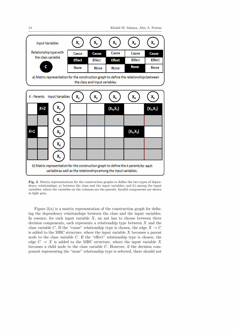
Fig. 2 Matrix representations for the construction graphs to define the two types of depen-dency relationships: a) between the class and the input variables; and b) among the inputvariables, where the variables on the columns are the parents. Invalid components are shownin light grey.
Figure 2(a) is a matrix representation of the construction graph for defin-ing the dependency relationships between the class and the input variables.In essence, for each input variable X, an ant has to choose between threedecision components, each represents a relationship type between X and theclass variable C. If the “cause” relationship type is chosen, the edge X → Cis added to the MBC structure, where the input variable X becomes a parentnode to the class variable C. If the “effect” relationship type is chosen, theedge C → X is added to the MBC structure, where the input variable Xbecomes a child node to the class variable C. However, if the decision com-ponent representing the “none” relationship type is selected, there should not
Title Suppressed Due to Excessive Length 15
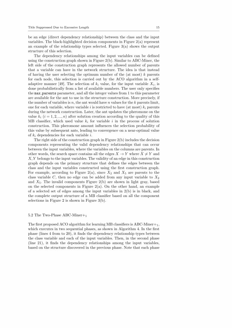
be an edge (direct dependency relationship) between the class and the inputvariables. The black-highlighted decision components in Figure 2(a) representan example of the relationship types selected. Figure 3(a) shows the outputstructure of this selection.
The dependency relationships among the input variables can be definedusing the construction graph shown in Figure 2(b). Similar to ABC-Miner, theleft side of the construction graph represents the allowed number of parentsthat a variable can have in the network structure. The idea is that insteadof having the user selecting the optimum number of the (at most) k parentsfor each node, this selection is carried out by the ACO algorithm in a self-adaptive manner [49]. The selection of ki value, for the input variable Xi, isdone probabilistically from a list of available numbers. The user only specifiesthe max parents parameter, and all the integer values from 1 to this parameterare available for the ant to use in the structure construction. More precisely, ifthe number of variables is n, the ant would have n values for the k parents limit,one for each variable, where variable i is restricted to have (at most) ki parentsduring the network construction. Later, the ant updates the pheromone on thevalue ki (i = 1, 2, ..., n) after solution creation according to the quality of thisMB classifier, which used value ki for variable i in the process of solutionconstruction. This pheromone amount influences the selection probability ofthis value by subsequent ants, leading to convergence on a near-optimal valueof ki dependencies for each variable i.
The right side of the construction graph in Figure 2(b) includes the decisioncomponents representing the valid dependency relationships that can occurbetween the input variables, where the variables on the columns are parents. Inother words, the search space contains all the edges X → Y where X = Y andX,Y belongs to the input variables. The validity of an edge in this constructiongraph depends on the primary structure that defines the edges between theclass and the input variables constructed using the first construction graph.For example, according to Figure 2(a), since X2 and X5 are parents to theclass variable C, then no edge can be added from any input variable to X2
and X5. The invalid components Figure 2(b) are shown in light gray, basedon the selected components in Figure 2(a). On the other hand, an exampleof a selected set of edges among the input variables in 2(b) is in black, andthe complete output structure of a MB classifier based on all the componentselections in Figure 2 is shown in Figure 3(b).
5.2 The Two-Phase ABC-Miner+1
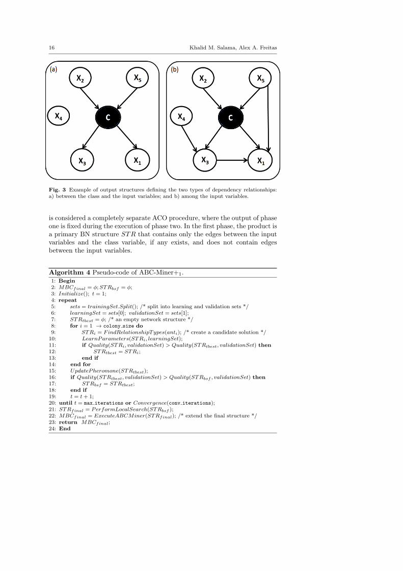
The first proposed ACO algorithm for learning MB classifiers is ABC-Miner+1,which executes in two sequential phases, as shown in Algorithm 4. In the firstphase (lines 4 from to 20), it finds the dependency relationship types betweenthe class variable and each of the input variables. Then, in the second phase(line 21), it finds the dependency relationships among the input variables,based on the structure discovered in the previous phase. Note that each phase
16 Khalid M. Salama, Alex A. Freitas
Fig. 3 Example of output structures defining the two types of dependency relationships:a) between the class and the input variables; and b) among the input variables.
is considered a completely separate ACO procedure, where the output of phaseone is fixed during the execution of phase two. In the first phase, the product isa primary BN structure STR that contains only the edges between the inputvariables and the class variable, if any exists, and does not contain edgesbetween the input variables.
Algorithm 4 Pseudo-code of ABC-Miner+1.1: Begin2: MBCfinal = ϕ;STRbsf = ϕ;3: Initialize(); t = 1;4: repeat5: sets = trainingSet.Split(); /* split into learning and validation sets */6: learningSet = sets[0]; validationSet = sets[1];7: STRtbest = ϕ; /* an empty network structure */8: for i = 1 → colony size do9: STRi = FindRelationshipTypes(anti); /* create a candidate solution */10: LearnParameters(STRi, learningSet);11: if Quality(STRi, validationSet) > Quality(STRtbest, validationSet) then12: STRtbest = STRi;13: end if14: end for15: UpdatePheromone(STRtbest);16: if Quality(STRtbest, validationSet) > Quality(STRbsf , validationSet) then17: STRbsf = STRtbest;18: end if19: t = t+ 1;20: until t = max iterations or Convergence(conv iterations);21: STRfinal = PerformLocalSearch(STRbsf );22: MBCfinal = ExecuteABCMiner(STRfinal); /* extend the final structure */23: return MBCfinal;24: End
Title Suppressed Due to Excessive Length 17
In essence, each anti in the colony constructs a candidate primary structureSTRi, using the FindRelationshipTypes() method (line 9). The constructionis performed by probabilistically selecting a relationship type for each inputvariable with respect to the class variable from the construction graph (asshown in Figure 2 (a)) according to the pheromone amounts associated withthe decision components. Then, the parameters are learnt for the structureusing the learning set (subset of the training set) to produce a BN classifier.The predictive quality of the produced model is evaluated on the validationset (a subset of the training set with no intersection with the learning set) andcompared with the iteration-best candidate solution STRtbest (lines 11 to 13).The pheromone update is performed according to the quality of STRtbest, inorder to influence the component selection of the ants during the constructionof the subsequent candidate solutions (line 15).
After that, the quality of the iteration-best solution STRtbest is comparedto the quality of the best-so-far solution STRbsf (lines 16 to 18), in order tokeep track of the best constructed primary structure. This set of steps is re-peated until the same solution is generated for a number of consecutive trialsspecified by the conv iterations parameter (indicating convergence) or untilmax iterations is reached (line 20). conv iterations, max iterations andcolony size are user-specified parameters. The best-so-far STRbsf structureundergoes local search, and the optimized primary STRfinal structure is pro-duced to be used in the next phase. Note that the BN structure discovered inthe first step contains no edges between the input variables, as shown in Figure3(a). The quality evaluation, local search, pheromone update, and training setsplit procedures are discussed in the following subsections.
In the second phase, the best constructed and optimized STRfinal struc-ture of the BN classifier is extended to a complete Markov blanket of the classvariable, by finding the dependency relationships among the input variables.To include this type of edge in the network structure, we execute the origi-nal ABC-Miner algorithm in this phase (line 22). However, in the context ofABC-Miner+1, the solution creation procedure (Algorithm 3) of ABC-Minerstarts with the STRfinal structure constructed in the previous phase, ratherthan a Naıve-Bayes structure as in the ABC-Miner algorithm (Algorithm 3,line 3). Therefore, the output of the procedure is a MB classifier, rather thana BAN.
5.3 The Integrated ABC-Miner+2
The second proposed ACO algorithm, ABC-Miner+2, employs an integratedapproach for building MB classifiers, where the relationships between the classand the input variables on one hand, and the relationships among the inputvariables on the other hand, are discovered in synergic fashion using a singlephase, as shown in Algorithm 5.

18 Khalid M. Salama, Alex A. Freitas
Algorithm 5 Pseudo-code of ABC-Miner+2.1: Begin2: MBCbsf = ϕ;3: Initialize(); t = 1;4: repeat5: sets = trainingSet.RandomSplit(); /* split into learning and validation sets */6: learningSet = sets[0]; validationSet = sets[1];7: STRtbest = ϕ; MBCtbest = ϕ;8: for i = 1 → colony size do9: STRi = FindRelationshipTypes(anti); /* wrt the class variable */10: LearnParameters(STRi, learningSet);11: if Quality(STRi, validationSet) > Quality(STRtbest, validationSet) then12: STRtbest = STRi;13: end if14: end for15: for i = 1 → colony size do16: MBCi = CreateSolution(anti, STRtbest); /* edges among input variables */17: if Quality(MBCi, validationSet) > Quality(MBCtbest, validationSet) then18: MBCtbest = MBCi;19: end if20: end for21: MBCtbest = PerformLocalSearch(MBCtbest);22: UpdatePheromone(MBCtbest);23: if Quality(MBCtbest, validationSet) > Quality(MBCbsf , validationSet) then24: MBCbsf = MBCtbest;25: end if26: t = t+ 1;27: until t = max iterations or Convergence(conv iterations);28: return MBCbsf ;29: End
Recall that the two-phase ABC-Miner+1 algorithm finishes the construc-tion of the primary BN structure (STR) that defines the edges between theclass and the input nodes, and fix this structure during the process of the sec-ond phase, which extends this structure by finding the edges between the inputnodes to complete the construction of a MB classifier (MBC). We can noticethat the ABC-Miner+1 has two separate repeat-until loops representing thesearch process of the ACO algorithms: 1) the one that produces the primarystructure STR (lines from 4 to 20 in Algorithm 4); and 2) the one that extendsthe primary structure to a complete MBC (in the execution of ABC-Miner,line 22 in Algorithm 4). By contrast, the ABC-Miner+2 algorithm consists ofone integrated repeat-until loop (lines from 4 to 27 in Algorithm 5), and ineach iteration of that loop a complete candidate MB classifier is constructed.
In each iteration of ABC-Miner+2, shown in Algorithm 5, the integratedconstruction of a candidate MBC is carried out in two steps, as follows. First,the ant colony responsible for creating candidate primary structures (usingthe construction graph shown in Figure 2(a)) constructs several candidateSTR solutions, using the FindRelationshipTypes() method, and selects theiteration-best STRtbest to go to the second step (lines 8 to 14). Then, theant colony responsible for extending a primary structure STR to a completeMB classifier MBC (using the construction graph shown in Figure 2(b)),
Title Suppressed Due to Excessive Length 19
extends the best discovered structure STRtbest in the previous step, usingthe CreateSolution() method, to construct several candidate complete MBCsolutions (lines 15 to 20).
The key integration aspect in this approach is that the pheromone updateis not performed on the two construction graphs until the complete MBC so-lution is constructed, local searched and evaluated. More precisely, in the firstphase of the ABC-Miner+1 algorithm, the pheromone feedback of the ants isperformed in each iteration according to the quality of the primary structure(line 15 in Algorithm 4), rather than a complete MB classifier. That is, the firstphase optimizes the primary structure, which defines the dependency relation-ships between the class and the input variables, independently of the possibledependency relationships that can be defined among the input variables. Onthe other hand, in the integrated approach of ABC-Miner+2, the pheromonefeedback is performed according to the quality (tested on a validation set) ofthe complete MB classifier (line 22 in Algorithm 5). The pheromone is up-dated on the decision components in the two construction graphs, introducinga relationship between the quality of the input variable-input variable depen-dency selection and the input variable-class dependency selections. Therefore,the optimization of the primary structure is also dependent on (or a part of)the optimization of the whole MB classifier structure.
5.4 A Note Regarding the Execution Time
The execution of the procedure shown in Algorithm 3, which adds the edgesbetween the input variables, is more efficient (faster) in the context of our twoproposed ACO algorithms (line 22 in Algorithm 4 and line 16 in Algorithm 5)than in the original ABC-Miner algorithm, which can be explained as follows.First, the search space of this procedure is smaller in the context of Algorithms4 and 5 than the search space in context of the original ABC-Miner. The reasonis that, in ABC-Miner, the initial structure is the Naıve-Bayes’ structure, whereall the input variables are children of the class variable, so all the candidateedges between the input variables are available for selection by an ant (i.e.,any variable can be a parent to any other variable).
On the other hand, in the proposed algorithms, the initial structure hassome input variables as parents of the class variable, and others are not evenrelated to the class variable. In this case, the candidate edges available for selec-tion to be added to the network are only the edges that satisfy two conditions,namely: the edge is connecting two input variables (rather than connecting aninput variable to the class), and the edge is pointing to a child node of theclass node. The algorithm does not consider adding edges between the classvariable’s parents because these edges do not affect the predictions (posteriorprobability calculation) of the MB classifier. For example, in Figure 2 (a),the valid edges to be added (white and black boxes) are the ones that arepointing to the variables X1 and X3, since they are the only child nodes to(effect of) the class variable, according to the previously constructed example
20 Khalid M. Salama, Alex A. Freitas
structure, as shown in Figure 3. Hence, line 22 in Algorithm 4 and line 16 inAlgorithm 5 call a somewhat modified version of Algorithm 3, where the onlymodified lines are the BAN initialization in line 3 and the implementation ofthe GetV alidEdges() procedure.
Second, in the MB models produced by our proposed ACO algorithms, thesize of the CPT for the variables that do not have the class variable as parentis relatively smaller compared to the CPT of the BN classifiers produced byABC-Miner, where the class node has to be a parent to all the variables, besidestheir other parents. Smaller CPT size leads to less computational time.
Note that both ABC-Miner+1 and ABC-Miner+2 perform the same (max-imum) number of solution quality evaluations, which represents the compu-tational budget of each algorithm, and is equal to max iterations timescolony size times 2. In the sequential two-phase ABC-Miner+1 (Algorithm4), the first half of the budget is utilized in the first phase (from line 4 toline 20), while the second half of the budget is utilized in the second phase(line 22). In ABC-Miner+2 (Algorithm 5), the whole computational budget isutilized in one, integrated phase (from line 4 to 27).
5.5 Local Search
In the context of the two phase ABC-Miner+1 algorithm, local search is per-formed in two different positions of the algorithm. The first position is atthe end of the first phase, where the local search is performed once on thebest-so-far primary structure STRbsf (line 21 in Algorithm 4), to produce theoptimized STRfinal that goes to phase two. In this procedure, the algorithmtries a different relationship type for each variable with respect to the classvariable. For example, if the relationship type between the input variable Xi
and the class variable C in the STRbsf is “cause”, the algorithm temporar-ily changes it: one time to “effect”, and another time to “none”. Then wecalculate the classification accuracy of each temporary BN structure (using avalidation set), and select the one with the highest quality. We perform thesame operations iteratively to each input variable Xi ∈ X. The best locallyoptimized structure STRfinal goes to the second phase.
In the second phase, the conventional local search procedure of ABC-Miner[49], embedded in the execution of line 22 of Algorithm 4, is performedafter each iteration. The procedure tentatively removes one edge between twoinput variables at a time from the constructed MBC in a reverse order (remov-ing last the edge that was added to the network first). If that removal improvesthe quality of the MB classifier, this edge is removed permanently from thenetwork; otherwise it is added once again. This process continues until all theedges between the input variables are tested to be removed from the MB clas-sifier, and then the MBCfinal with the highest quality is returned. Note thatthe local search of the second phase does not affect the primary structure (theedges between the class and the input variables) discovered and optimized inthe first phase.

Title Suppressed Due to Excessive Length 21
In the integrated ABC-Miner+2, the local search procedure is performedin one position in the algorithm (line 21 in Algorithm 5). In each iterationt, the iteration-best constructed MB classifier MBCtbest undergoes the localsearch as follows. First, the edges between the input variables are temporarilyremoved, one edge at a time, in a reversed order, where the edges whoseremoval improves the quality of the MBCtbest (tested on a validation set) areremoved permanently from the structure. Next, the edges between the classand the input variables are tested to be removed, that is, for each variablethat has a dependency relationship to the class variable other that “none”, wetemporarily change it to “none”. This is performed for one variable at a timefor each valid variable, where the change is kept if it improves the quality ofthe MB classifier.
We can notice that the second part of this local search procedure (involv-ing the edges between the class and the input variables) is simpler than itscorresponding procedure in ABC-Miner+1 that optimizes the primary struc-ture STRbsf , since only the “none” relationship type is tried for only a subsetof variables (which have edges with the class), rather than trying the othertwo relationship types for each variable. This is intended for two reasons. Thefirst reason is to reduce the computational time, since this procedure is calledin each iteration in ABC-Miner+2, (line 21 in Algorithm 5), unlike ABC-Miner+1, which calls the local search procedure only once on the best-so-farconstructed primary structure (line 20 in Algorithm 4).
The second reason is that changing the relationship type from “cause” to“effect” or vice versa, after adding a dependency relationship among the inputvariables, may introduce irrelevant edges in the MBC structure. For example,suppose that X and Y are input variables, and there is a dependency relation-ship between them: X → Y . Suppose that the relationship type between Yand the class variable C is “effect”, i.e., the edge is C → Y . Now suppose wechange the relationship type from “effect” to “cause”, i.e., the edge becomesC ← Y . In this case, the dependency relationship X → Y between X and Ybecomes irrelevant to the class variable prediction and outside the scope ofthe class variable’s Markov blanket.
5.6 Solution Quality Evaluation
As discussed in Section 4.2, GBN algorithms do not recognize any specialtarget class variable. They treat all the variables of the dataset in the sameway, and they are used to answer all types of inference queries about any setof variables, which may or may not include the class variable. By contrast, aBN classifier is only concerned about the queries regarding the class variable,and so the BN classification algorithm should be designed to build a modelthat maximizes its effectiveness concerning the prediction of the target classvariable.
Taking into account the aforementioned argument, ABC-Miner evaluatesthe quality of a candidate BN during the training phase directly as a classifier,
22 Khalid M. Salama, Alex A. Freitas
using the accuracy measure as the indicator of the predictive performance ofthat classifier. Accuracy is a simple and yet popular predictive performancemeasure, computed as:
Accuracy =|Correct||V Set|
, (6)
where Correct is the set of the correctly classified instances, and V Set is thecurrent validation set.
However, the conventional accuracy measure discards the fact that a BNclassifier does not only predict a class label of any given instance, it also as-sociates a probability to this predicted class label. This probability representsthe confidence of the BN classifier regarding its prediction.
More precisely, suppose we have two candidate BN classifiers BNC1 andBNC2, which are used to classify instance X l, where l is the correct class labelof the instance. Now let us assume that the posterior probabilities of the classC given instance X and each BN classifier are (C = l|X l, BNC1)=0.9 and(C = l|X l, BNC2)=0.55. If we used accuracy as the predictive performancemeasure, instance X l will be counted as 1 correctly classified instance for bothBN classifiers, and the performance of the two classifiers would be equal (withrespect to the classification of instance X). However, this discards the factthat BNC1 produced a higher posterior probability of the correct class labelthan the one produced by BNC2. Therefore, during the training phase, BNC1
should be considered to have a higher quality than BNC2, and consequentlyshould receive a better pheromone feedback.
We have addressed such an issue in our ACO algorithms for learning MBclassifiers, where we used probabilistic accuracy to evaluate the quality of thecandidate constructed MBC solutions and perform pheromone update. Asshown in Equation 7, the probabilistic accuracy will count each of the classifiedinstances in the validation set according to the posterior probability of itscorrect class label produced by the candidate MB classifier.
Probabilistic Accuracy =
∑|V Set|j P (C = l|X l
j)
|V Set|, (7)
where X lj is the j-th instance in the validation set, and l is the correct class
label of instance Xj . Note that the probabilistic accuracy (Equation 7) isonly the first component of the quality measure used to evaluate a candidateMB classifier. The second component, which concerns mitigating overfitting,is described in the next subsection.
As for pheromone update, we use the same procedure employed by theABC-Miner algorithm [49]. Concerning pheromone deposit, the pheromoneamount is increased on each decision component according to the quality oftwo constructed solutions: the iteration-best tbest and the best-so-far bsf us-ing a weighted reinforcement strategy. The strategy aims at focusing on theexploration aspect during the early iterations in the algorithms by giving more

Title Suppressed Due to Excessive Length 23
weight to the tbest solution in depositing pheromone. Gradually, the proce-dure moves to exploitation as the search progresses by giving more weight tothe bsf in depositing pheromone, leading to convergence towards a good so-lution. Then, the pheromone amounts are normalized to simulate pheromoneevaporation [49].
5.7 Overfitting Mitigation
A key objective of a classification algorithm is to learn models with good gen-eralization capabilities, i.e., models that are able to accurately predict the classlabels of previously unknown instances. In fact, the available instances in thedataset used for building and validating a classification model are consideredjust a sample of a larger population of possible instances in the applicationdomain of concern. The aim is to build a model that can generalize over thecurrent dataset to correctly fit the data of the whole application domain asmuch as possible [22,52].
Overfitting occurs when the induced model (classifier) reflects good clas-sification performance (fit) on the training (in-sample) data used for in thelearning process, yet shows bad predictive performance (generalization) in-volving new/testing data. This is in general a property of complex classifiersthat have a high degree of freedom — i.e., a BN classifier with a large num-ber of dependency relationships (edges). In general, overfitting can occur dueto two factors. First, if the classification algorithm used the whole trainingdataset for both learning (building the model) and validating the model’s ac-curacy. In this case, the generalization ability would not be tested during thetraining phase, since the model would be validated on the same instances usedto learn that model. The quality of the induced classifier might be due to ahigh (undesirable) fit on the training set, and the same classifier might showa bad predictive accuracy on the unseen test (out-of-sample) dataset. Second,allowing the classification algorithm to build too complex models might lead itto learn an over-tuned model that “memorizes” the training data, which harmsits generalization ability. Learning, in the sense of using a set of instances tobuild a classifier that can predict the class of unseen instances, needs induction,which refers to discovering a general hypothesis (classification model) that candescribe both the sample instances at hand and the whole population of theinstances in the application domain as well [38,52].
In the context of our proposed algorithms, we tried to mitigate the over-fitting problem, to produced well-generalized MB classification models, as fol-lows. First, in order not to allow building complex BN structures, we limitedthe maximum number of parents that each node can have in the network to3 (as applied in ABC-Miner [45,49]). However, learning MBC models is moreprone to overfitting than learning BANs, since in the class variable MB struc-ture, the class can have input variables as parents. In an extreme case, if theclass variable would have all the input variables as its parents, the producedmodel would be perfectly memorizing the training data in the parameters of

24 Khalid M. Salama, Alex A. Freitas
the constructed BMC. More precisely, one big CPT would be built for the classvariable that stores the probability of each class label given each combinationof the input variables, which is an undesirable behavior.
We have noticed that, the more parent nodes the class variable has, themore it is prone to overfitting. Therefore, we introduced a penalty compo-nent to the quality evaluation formula, which affects the pheromone updateprocedure, based on the number of parents of the class variables, as follows:
Quality(MBC) = ProbabAcc(MBC, validation set)− Penalty(MBC), (8)
Penalty(MBC) =1
2(n−p), (9)
where ProbabAcc() refers to the probabilistic accuracy measure that is shownin Equation 7, p is the number of parent nodes to the class variables, and n isthe total number of the input variables. Note that Equation 8 represents thecomplete formula for evaluating a candidate MBC solution quality to performpheromone update.
As shown in Equation 9, the penalty value can range from 0 to 1 (the samerange as the probabilistic accuracy), according to the number of parents thatthe class variable has. If all the input variables are parents to the class node(i.e., p = n) – which is totally undesirable, the penalty value would be themaximum (equals 1), and the total quality value of the model according toEquation 8 would be less than or equal to 0. However, if the p = n − 1, thepenalty would be reduced to its half. This means that, according to Equation9, adding one more parent to the class variable would double the penaltyvalue, as it would be increasing the possibility of the MBC model to overfitthe training data.
Second, instead of having the algorithm build the MB classifier over thewhole training set, the training set is split into two mutually exclusive parts:1) the learning set, which contains 75% of the training set and is used tobuild a candidate MBC (i.e., BN parameter learning, as shown in Algorithm4, line 10 and Algorithm 5, lines 10 and 16); and 2) the validation set, whichcontains 25% of the training set and is used to evaluate the quality of theconstructed MBC for pheromone update. Such a strategy is common in manyclassification algorithms. However, these two parts are usually fixed during thewhole training process, which may lead to optimize the model constructionover the validation set. To avoid that the model overfits a fixed validation set,we propose randomly changing the partitioning of the learning/validation setsin each iteration, in order to push the generalization ability of the constructedmodels over any part of the training set. In our experiments, we utilize thisidea in the two versions of ABC-Miner+ (as shown in Algorithm 4 and 5, lines5 to 6), as well as in the original ABC-Miner algorithm.

Title Suppressed Due to Excessive Length 25
6 Experimental Methodology
6.1 Comparative Evaluations
We compare the predictive accuracy of our proposed ACO algorithms for learn-ing MB classifiers with our previously introduced ABC-Miner that learns BANclassifiers, as well as three other widely used Bayesian Network (BN) classi-fiers, namely Naıve-Bayes, Tree Augmented Naıve-Bayes (TAN) and GeneralBayesian Network (GBN). A variation of the Chow-Liu (CL) tree algorithm[3] is used for building TANs, as follows. First, it computes the conditionalmutual information I(X,Y |C) between each pair of variables X and Y givenclass variable C. Then it builds a complete undirected graph connecting all theinput variables to find the maximum weighted spanning tree from the graph,where the weight of the edge X → Y is annotated with I(X,Y |C). After that,it chooses a root variable and sets the direction of all edges to be outwards ofit. Finally, it adds one edge from the class node to each of the other variablesto complete a TAN classifier. As for the construction of GBNs, Algorithm-B[2] is used to build a general Bayesian network. The algorithm utilizes a greedysearch to optimize the K2 scoring function for the Bayesian network. Then,the Markov blanket of the class node is extracted from the BN to be used asa MB classifier. We implemented in the experiments another version of theGBN learning algorithm, which optimizes the predictive accuracy, denoted asGHC-Acc. That is, it starts with an edge-less BN structure, and incrementallyadds the edge which leads to the highest increase in classification accuracyon the validation set. Table 1 presents the main properties of the used BNclassification algorithms.
Table 1 Summary of the BN classification algorithms used in the experiments.
Algorithm Type Search Strategy Output Optimization
Naıve-Bayes Determ. - NB -
CL-Tree Determ. Max. Spanning Tree TAN Cond. Mut. Info.
Algorithm-B Determ. Greedy Hill Clim. GBN K2 Function
GHC-Acc Determ. Greedy Hill Clim. GBN Predictive Acc.
ABC-Miner Stoch. Ant Colony Optim. BAN Predictive Acc.
ABC-Miner+1 Stoch. Ant Colony Optim. MBC Probabilistic Acc.
ABC-Miner+2 Stoch. Ant Colony Optim. MBC Probabilistic Acc.
Besides the BN classification algorithms, we compare our proposed ACOalgorithms with three well-known classification algorithms: Ripper, C4.5, andSVM [53]. Ripper is a classification rule induction algorithm, which learns aclassification model that consists of a list of classification rules, where eachrule has the form: “IF (Antecedent) THEN (Class)”. C4.5 builds classificationdecision trees, where the internal nodes are the input attribute values of thedataset, and the leaf nodes are the classes to be predicted. An SVM maps
26 Khalid M. Salama, Alex A. Freitas
the instances into a higher-dimensional feature space and then finds the besthyper-plane for separating instances of different classes – where the best hyper-plane is the one with the greatest possible margin (a gap separating instancesof different classes in the data space). Note that SVMs have the disadvantageof producing black-box classification models that can hardly be interpreted byusers [53,17,16], unlike the other types of classifiers used in our experiments.
6.2 Experimental Setup
The experiments were carried out using stratified 10-fold cross validation [53].For the stochastic ACO-based algorithms, we run each algorithm 10 times– using a different random seed to initialize the search each time – for eachcross-validation fold. In the case of the deterministic algorithms, each is runjust once for each fold.
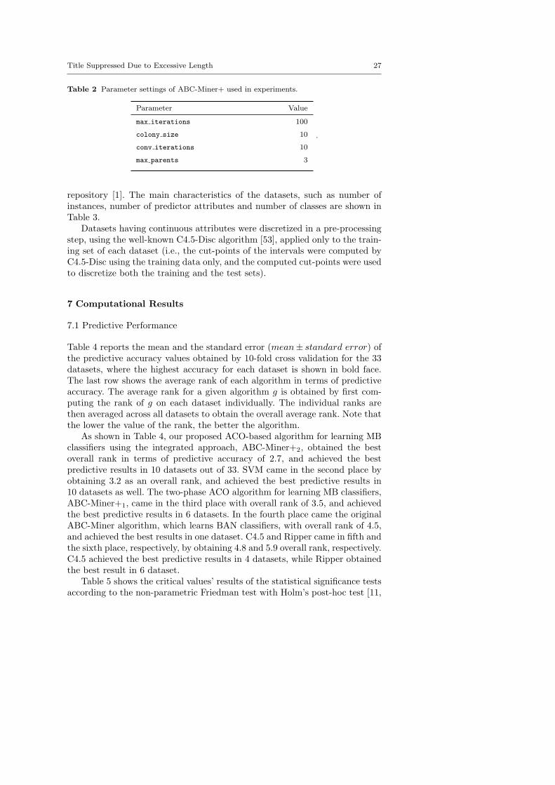
The parameter configuration used in our experiments is shown in Table2. Note that the max iterations parameter refers to the maximum numberof iterations used in ABC-Miner and ABC-Miner+2. However, in the case ofthe two-phase ABC-Miner+1, each phase is allocated half of the total max-imum number of iterations (i.e. 500 iterations in our experiments). On theother hand, for the greedy Algorithm-B and GHC-Acc algorithms, we re-fer to max iterations as the maximum number of solution evaluations thatthe algorithm performs during the hill-climbing search to build a GBN. Itis set to 1000, which is equal to the value of max iterations multiplied bycolony size used for our stochastic ant-based algorithms. For the sake of faircomparison, we limit each algorithm to the same fixed number of solution eval-uations to construct the model. However, the maximum number might not beutilized completely; ACO-based algorithms might only use a smaller numberof iterations if they converged earlier and the greedy-based algorithms mightalso stop earlier if they get stuck in a local optimum.
Unlike our ant-based algorithms, the number of parents (k-dependencies)must be specified for Algorithm-B and GHC-Acc. We set it to 3, which is themaximum number of parents used in our ACO algorithm, where the numberof parents is selected dynamically at each iteration (see Section 5.1). Notealso that we have employed the two overfitting mitigation procedures (i.e.,adding the penalty component in the quality evaluation function and randomlysplitting the training set into a learning set and a validation set each iteration),discussed in Section 5.7, in both versions of the ABC-Miner+ algorithm. Asfor the other classification algorithms, in our experiments, we used WEKA[53] implementations for Rippper (JRip), C4.5 (J48), and SVM (SMO), eachwith its default parameter settings.
6.3 Evaluation Datasets
The performance of ABC-Miner+1 and ABC-Miner+2 was evaluated using 33public-domain datasets from the University of California at Irvine UCI dataset
Title Suppressed Due to Excessive Length 27
Table 2 Parameter settings of ABC-Miner+ used in experiments.
Parameter Value
max iterations 100
colony size 10
conv iterations 10
max parents 3
.
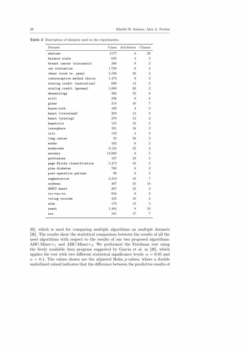
repository [1]. The main characteristics of the datasets, such as number ofinstances, number of predictor attributes and number of classes are shown inTable 3.
Datasets having continuous attributes were discretized in a pre-processingstep, using the well-known C4.5-Disc algorithm [53], applied only to the train-ing set of each dataset (i.e., the cut-points of the intervals were computed byC4.5-Disc using the training data only, and the computed cut-points were usedto discretize both the training and the test sets).
7 Computational Results
7.1 Predictive Performance
Table 4 reports the mean and the standard error (mean± standard error) ofthe predictive accuracy values obtained by 10-fold cross validation for the 33datasets, where the highest accuracy for each dataset is shown in bold face.The last row shows the average rank of each algorithm in terms of predictiveaccuracy. The average rank for a given algorithm g is obtained by first com-puting the rank of g on each dataset individually. The individual ranks arethen averaged across all datasets to obtain the overall average rank. Note thatthe lower the value of the rank, the better the algorithm.
As shown in Table 4, our proposed ACO-based algorithm for learning MBclassifiers using the integrated approach, ABC-Miner+2, obtained the bestoverall rank in terms of predictive accuracy of 2.7, and achieved the bestpredictive results in 10 datasets out of 33. SVM came in the second place byobtaining 3.2 as an overall rank, and achieved the best predictive results in10 datasets as well. The two-phase ACO algorithm for learning MB classifiers,ABC-Miner+1, came in the third place with overall rank of 3.5, and achievedthe best predictive results in 6 datasets. In the fourth place came the originalABC-Miner algorithm, which learns BAN classifiers, with overall rank of 4.5,and achieved the best results in one dataset. C4.5 and Ripper came in fifth andthe sixth place, respectively, by obtaining 4.8 and 5.9 overall rank, respectively.C4.5 achieved the best predictive results in 4 datasets, while Ripper obtainedthe best result in 6 dataset.
Table 5 shows the critical values’ results of the statistical significance testsaccording to the non-parametric Friedman test with Holm’s post-hoc test [11,
28 Khalid M. Salama, Alex A. Freitas
Table 3 Description of datasets used in the experiments.
Dataset Cases Attributes Classes
abalone 4177 8 29
balance scale 625 4 3
breast cancer (wisconsin) 286 9 2
car evaluation 1,728 6 4
chess (rook vs. pawn) 3,196 36 2
contraceptive method choice 1,473 9 3
statlog credit (australian) 690 14 2
statlog credit (german) 1,000 20 2
dermatology 366 33 6
ecoli 336 8 8
glass 214 10 7
hayes-roth 160 4 3
heart (cleveland) 303 12 3
heart (statlog) 270 13 2
hepatitis 155 19 2
ionosphere 351 34 2
iris 150 4 3
lung cancer 32 56 3
monks 432 6 2
mushrooms 8,124 22 2
nursery 12,960 8 5
parkinsons 197 23 2
page Blocks classification 5,473 10 5
pima diabetes 768 8 2
post-operative patient 90 8 3
segmentation 2,310 19 7
soybean 307 35 19
SPECT heart 267 22 2
tic-tac-to 958 9 2
voting records 435 16 2
wine 178 13 3
yeast 1,484 8 10
zoo 101 17 7
20], which is used for comparing multiple algorithms on multiple datasets[26]. The results show the statistical comparison between the results of all theused algorithms with respect to the results of our two proposed algorithms:ABC-Miner+1 and ABC-Miner+2. We performed the Friedman test usingthe freely available Java program suggested by Garcia et al. in [20], whichapplies the test with two different statistical significance levels: α = 0.05 andα = 0.1. The values shown are the adjusted Holm p-values, where a doubleunderlined valued indicates that the difference between the predictive results of
Title Suppressed Due to Excessive Length 29
the two corresponding algorithms in the table is statistically significant at 5%level, and a single underlined value indicates that the difference is statisticallysignificant at 10% level. A result shown with no underlines indicates that thereis no statistically significant difference between predictive performances of thecorresponding algorithms.

30 Khalid M. Salama, Alex A. FreitasTable
4Predictiveaccuracy
%(m
ean±
standarder
ror)resu
lts.
Data
set
Naıve-B
Cl-Tree
Algo-B
GHC-A
cc
ABC-M
iner
JRip
J48
SVM
ABC-M
iner+
1ABC-M
iner+
2
abl
86.1
±2.5
87.2
±1.6
88.3
±1.3
88.7
±2.7
85.6
±2.7
92.6
±2.5
92.6
±2.1
89.1
±1.2
88.7
±1.5
89.3
±1.8
bal
91.2
±0.8
84.4
±0.9
85.6
±0.6
83.4
±0.9
84.7
±0.7
77.6
±1.8
80.2
±1.2
88.4
±0.9
85.6
±0.9
86.8
±0.7
bcw
92.1
±1.4
95.4
±1.2
93.8
±2.7
94.6
±1.4
95.4
±2.5
94.7
±1.5
95.1
±2.5
97.7
±1.7
95.4
±1.5
97.6
±2.7
car
85.3
±2.2
93.6
±1.2
86.2
±1.3
92.1
±2.1
97.2
±2.3
90.6
±1.2
94.3
±2.8
94.1
±2.5
98.1
±1.1
98.6
±2.4
chess
88.2
±1.5
92.5
±1.4
89.8
±2.2
95.1
±2.2
97.6
±2.5
98.1
±1.5
98.4
±2.3
95.1
±1.8
96.3
±2.7
97.6
±2.5
cmc
52.2
±2.1
56.4
±2.2
54.6
±2.8
60.4
±2.8
66.4
±2.7
60.1
±1.1
64.2
±2.4
60.2
±2.2
67.8
±2.8
65.3
±2.2
crd-a
77.5
±2.6
85.1
±1.8
85.7
±1.4
85.2
±2.4
86.8
±2.6
85.7
±2.5
91.9
±1.2
85.5
±1.1
84.2
±2.1
87.1
±2.6
crd-g
75.6
±1.6
73.7
±1.8
75.6
±1.2
74.8
±2.3
73.7
±2.8
73.2
±1.8
75.7
±1.6
75.2
±2.3
75.8
±2.7
77.6
±1.1
drm
96.2
±1.5
97.8
±1.1
97.2
±1.6
96.0
±2.6
98.6
±2.6
94.8
±2.7
96.1
±1.8
97.2
±2.1
99.0
±1.3
97.7
±2.8
ecoli
86.5
±2.2
84.2
±2.7
82.6
±2.6
84.1
±1.4
87.4
±1.2
84.3
±1.7
85.7
±2.8
87.6
±1.6
90.4
±1.2
90.4
±2.4
glass
74.2
±1.1
78.4
±0.9
80.7
±1.2
80.9
±2.3
82.6
±2.7
75.7
±1.4
82.2
±1.2
82.6
±1.2
85.3
±2.4
85.8
±1.5
hay
80.0
±1.4
77.9
±1.7
83.1
±2.7
84.2
±2.1
80.2
±2.3
84.2
±2.1
83.3
±2.3
81.6
±2.7
82.4
±2.1
84.2
±1.4
hrt-c
62.7
±2.1
68.8
±2.5
66.7
±1.7
76.8
±2.6
83.8
±2.1
67.1
±2.1
70.9
±2.3
72.6
±1.8
84.2
±2.5
81.8
±1.6
hrt-s
83.4
±1.7
83.3
±2.4
81.5
±1.8
72.4
±2.7
85.6
±2.4
76.6
±1.6
75.5
±1.8
84.1
±2.3
88.4
±2.7
86.2
±2.6
hep
71.9
±1.6
78.0
±1.6
67.3
±2.1
74.2
±1.6
77.8
±1.2
72.7
±1.4
68.9
±1.2
74.2
±1.6
78.6
±0.9
78.0
±1.6
iono
82.6
±0.6
90.5
±1.5
90.5
±1.5
92.8
±1.2
94.5
±1.7
92.8
±1.3
93.1
±2.7
95.8
±1.7
94.9
±1.3
94.9
±1.1
iris
96.2
±2.8
94.2
±1.2
92.9
±2.2
96.2
±2.8
96.2
±1.7
95.6
±1.8
95.0
±2.5
96.6
±2.1
96.2
±1.1
96.2
±2.5
lung
72.5
±2.6
75.4
±2.7
63.2
±1.8
74.8
±2.2
74.8
±2.8
58.7
±1.3
75.7
±1.5
79.3
±2.2
74.8
±1.2
74.3
±2.2
monk
61.6
±2.3
58.8
±2.4
61.6
±2.1
61.6
±1.1
61.8
±1.1
61.4
±1.2
62.2
±1.6
63.3
±1.3
62.2
±1.2
64.6
±2.7
mush
95.8
±1.7
98.2
±1.5
96.1
±2.8
98.0
±2.3
98.8
±2.4
100
±2.3
100
±1.7
100
±2.4
99.9
±2.3
99.9
±1.3
nurs
90.1
±1.7
94.3
±1.6
92.7
±2.7
93.1
±2.6
98.0
±1.4
96.5
±2.8
97.1
±1.8
93.2
±2.7
97.7
±1.2
98.2
±2.5
park
84.5
±2.2
91.7
±1.7
84.5
±1.2
88.2
±2.5
94.2
±2.1
98.5
±1.8
96.2
±2.4
98.2
±1.4
98.5
±2.4
98.7
±2.8
pbc
93.5
±1.7
96.1
±1.4
95.6
±1.1
94.2
±2.4
96.5
±2.1
97.4
±1.5
98.2
±2.6
98.7
±2.3
97.8
±2.2
96.5
±2.4
pima
75.4
±1.2
77.8
±1.5
76.2
±1.5
76.2
±1.5
78.9
±1.9
79.9
±1.9
79.5
±1.6
75.7
±1.2
78.9
±1.9
78.9
±1.9
pop
68.2
±2.3
64.1
±2.2
66.6
±2.1
71.1
±2.1
74.3
±2.4
71.1
±1.7
71.1
±1.7
72.2
±1.7
70.3
±1.7
72.5
±1.2
seg
91.6
±1.4
94.8
±2.6
94.1
±2.7
94.0
±1.2
94.5
±2.1
94.7
±2.4
96.3
±2.5
97.8
±2.7
95.8
±2.8
971.±
1.3
soy
91.4
±1.7
95.6
±2.4
93.2
±2.2
92.1
±1.7
95.6
±1.1
91.5
±1.7
95.1
±2.3
97.6
±1.4
95.6
±1.3
95.6
±1.2
SPECT
73.7
±2.7
72.1
±1.4
74.0
±2.6
76.5
±2.6
76.5
±2.6
76.7
±2.2
74.4
±1.1
78.5
±1.5
78.8
±2.4
79.6
±2.6
ttt
70.3
±1.5
76.6
±2.5
74.3
±2.1
82.5
±2.5
86.4
±2.4
97.8
±1.5
85.7
±2.3
96.3
±2.3
86.8
±1.4
89.2
±2.3
vot
90.3
±1.6
92.1
±1.5
90.3
±1.8
91.4
±1.7
94.6
±1.5
96.5
±2.1
96.3
±2.6
95.8
±2.2
95.6
±2.7
95.6
±1.5
wine
95.6
±1.4
97.3
±1.3
97.3
±1.3
98.8
±2.2
98.4
±1.7
97.6
±1.1
95.8
±2.4
98.9
±1.7
98.0
±1.3
98.4
±1.1
yeast
59.7
±2.7
61.2
±1.8
60.2
±2.2
61.5
±1.8
62.6
±2.4
63.8
±1.5
64.2
±1.2
64.6
±1.7
64.2
±1.6
64.5
±1.7
zoo
94.2
±1.2
97.3
±1.3
95.1
±1.8
96.2
±1.2
97.0
±1.7
94.2
±2.5
96.1
±1.4
97.5
±2.2
97.0
±1.2
97.0
±2.1
Rank
8.6
6.8
8.0
6.7
4.5
5.9
4.8
3.2
3.5
2.7

Title Suppressed Due to Excessive Length 31
Table 5 The non-parametric Friedman statistical test results (adjusted p-values) withHolm’s post-hoc correction.
Algorithm ABC-Miner+1 ABC-Miner+2
Naıve-Bayes 7.8E-1 1.9E-13
CL-Tree 3.3E-4 1.2E-6
Algorithm-B 3.4E-7 2.4E-10
GHC-Acc 0.0023 1.4E-5
ABC-Miner 1.0 0.0946
Ripper 0.0681 0.0012
C4.5 1.0 0.08012
SVM 1.0 1.0
7.2 Model Simplicity
Table 6 reports the model size results – in terms of the number of edges –of the models produced by the BN classification algorithms, as the averageof the 10-fold cross validation experiments. The last row in the table showsthe average rank of results for the model sizes over all the datasets, where thelower the rank, the better the algorithm. Note that we do not report the sizeresults for Naıve-Bayes, since it is obvious that it produces the smallest modelsize; a Naıve-Bayes model has a number of edges that is equal to the numberof input variables in the dataset.
As shown in Table 6, TAN, as expected, produces the smallest BN modelsin general, since the number of parents for each node in a TAN is restrictedto one, besides the class parent. The reason why in some cases the ACO-based algorithm produces smaller models is due to the local search procedurethat might remove edges. We can also see that, in most of the datasets, theMB classifier structures produced by our proposed ACO algorithms are smallerthan the BAN models produced by ABC-Miner. More precisely, ABC-Miner+1
and ABC-Miner+2 obtained overall rankings of 2.3 and 3.1, respectively, whileABC-Miner obtained overall ranking of 4.3 (coming in the last place).
7.3 Execution Time
The execution time results are shown in Table 7. The running time (in seconds)of each algorithm in each dataset is reported. Besides, the ratio of the runningtime of each algorithm to the ABC-Miner algorithm (as a baseline) is shown inthe column with ”ratio” header in bold face. The last row in the table reportsthe average ratio of the running time of each algorithm to ABC-Miner acrossall the datasets. All the experiments were performed with an Intel dual-core i7
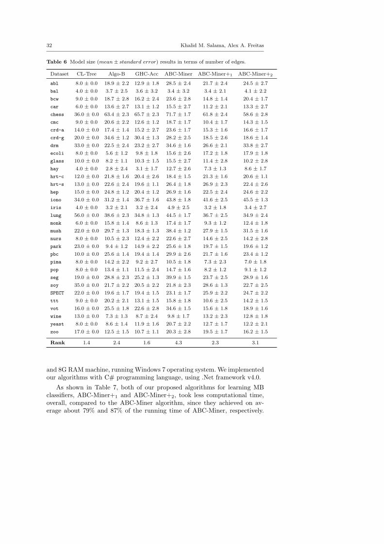
32 Khalid M. Salama, Alex A. Freitas
Table 6 Model size (mean± standard error) results in terms of number of edges.
Dataset CL-Tree Algo-B GHC-Acc ABC-Miner ABC-Miner+1 ABC-Miner+2
abl 8.0 ± 0.0 18.9 ± 2.2 12.9 ± 1.8 28.5 ± 2.4 21.7 ± 2.4 24.5 ± 2.7
bal 4.0 ± 0.0 3.7 ± 2.5 3.6 ± 3.2 3.4 ± 3.2 3.4 ± 2.1 4.1 ± 2.2
bcw 9.0 ± 0.0 18.7 ± 2.8 16.2 ± 2.4 23.6 ± 2.8 14.8 ± 1.4 20.4 ± 1.7
car 6.0 ± 0.0 13.6 ± 2.7 13.1 ± 1.2 15.5 ± 2.7 11.2 ± 2.1 13.3 ± 2.7
chess 36.0 ± 0.0 63.4 ± 2.3 65.7 ± 2.3 71.7 ± 1.7 61.8 ± 2.4 58.6 ± 2.8
cmc 9.0 ± 0.0 20.6 ± 2.2 12.6 ± 1.2 18.7 ± 1.7 10.4 ± 1.7 14.3 ± 1.5
crd-a 14.0 ± 0.0 17.4 ± 1.4 15.2 ± 2.7 23.6 ± 1.7 15.3 ± 1.6 16.6 ± 1.7
crd-g 20.0 ± 0.0 34.6 ± 1.2 30.4 ± 1.3 28.2 ± 2.5 18.5 ± 2.6 18.6 ± 1.4
drm 33.0 ± 0.0 22.5 ± 2.4 23.2 ± 2.7 34.6 ± 1.6 26.6 ± 2.1 33.8 ± 2.7
ecoli 8.0 ± 0.0 5.6 ± 1.2 9.8 ± 1.8 15.6 ± 2.6 17.2 ± 1.8 17.9 ± 1.8
glass 10.0 ± 0.0 8.2 ± 1.1 10.3 ± 1.5 15.5 ± 2.7 11.4 ± 2.8 10.2 ± 2.8
hay 4.0 ± 0.0 2.8 ± 2.4 3.1 ± 1.7 12.7 ± 2.6 7.3 ± 1.3 8.6 ± 1.7
hrt-c 12.0 ± 0.0 21.8 ± 1.6 20.4 ± 2.6 18.4 ± 1.5 21.3 ± 1.6 20.6 ± 1.1
hrt-s 13.0 ± 0.0 22.6 ± 2.4 19.6 ± 1.1 26.4 ± 1.8 26.9 ± 2.3 22.4 ± 2.6
hep 15.0 ± 0.0 24.8 ± 1.2 20.4 ± 1.2 26.9 ± 1.6 22.5 ± 2.4 24.6 ± 2.2
iono 34.0 ± 0.0 31.2 ± 1.4 36.7 ± 1.6 43.8 ± 1.8 41.6 ± 2.5 45.5 ± 1.3
iris 4.0 ± 0.0 3.2 ± 2.1 3.2 ± 2.4 4.9 ± 2.5 3.2 ± 1.8 3.4 ± 2.7
lung 56.0 ± 0.0 38.6 ± 2.3 34.8 ± 1.3 44.5 ± 1.7 36.7 ± 2.5 34.9 ± 2.4
monk 6.0 ± 0.0 15.8 ± 1.4 8.6 ± 1.3 17.4 ± 1.7 9.3 ± 1.2 12.4 ± 1.8
mush 22.0 ± 0.0 29.7 ± 1.3 18.3 ± 1.3 38.4 ± 1.2 27.9 ± 1.5 31.5 ± 1.6
nurs 8.0 ± 0.0 10.5 ± 2.3 12.4 ± 2.2 22.6 ± 2.7 14.6 ± 2.5 14.2 ± 2.8
park 23.0 ± 0.0 9.4 ± 1.2 14.9 ± 2.2 25.6 ± 1.8 19.7 ± 1.5 19.6 ± 1.2
pbc 10.0 ± 0.0 25.6 ± 1.4 19.4 ± 1.4 29.9 ± 2.6 21.7 ± 1.6 23.4 ± 1.2
pima 8.0 ± 0.0 14.2 ± 2.2 9.2 ± 2.7 10.5 ± 1.8 7.3 ± 2.3 7.0 ± 1.8
pop 8.0 ± 0.0 13.4 ± 1.1 11.5 ± 2.4 14.7 ± 1.6 8.2 ± 1.2 9.1 ± 1.2
seg 19.0 ± 0.0 28.8 ± 2.3 25.2 ± 1.3 39.9 ± 1.5 23.7 ± 2.5 28.9 ± 1.6
soy 35.0 ± 0.0 21.7 ± 2.2 20.5 ± 2.2 21.8 ± 2.3 28.6 ± 1.3 22.7 ± 2.5
SPECT 22.0 ± 0.0 19.6 ± 1.7 19.4 ± 1.5 23.1 ± 1.7 25.9 ± 2.2 24.7 ± 2.2
ttt 9.0 ± 0.0 20.2 ± 2.1 13.1 ± 1.5 15.8 ± 1.8 10.6 ± 2.5 14.2 ± 1.5
vot 16.0 ± 0.0 25.5 ± 1.8 22.6 ± 2.8 34.6 ± 1.5 15.6 ± 1.8 18.9 ± 1.6
wine 13.0 ± 0.0 7.3 ± 1.3 8.7 ± 2.4 9.8 ± 1.7 13.2 ± 2.3 12.8 ± 1.8
yeast 8.0 ± 0.0 8.6 ± 1.4 11.9 ± 1.6 20.7 ± 2.2 12.7 ± 1.7 12.2 ± 2.1
zoo 17.0 ± 0.0 12.5 ± 1.5 10.7 ± 1.1 20.3 ± 2.8 19.5 ± 1.7 16.2 ± 1.5
Rank 1.4 2.4 1.6 4.3 2.3 3.1
and 8G RAMmachine, running Windows 7 operating system. We implementedour algorithms with C# programming language, using .Net framework v4.0.
As shown in Table 7, both of our proposed algorithms for learning MBclassifiers, ABC-Miner+1 and ABC-Miner+2, took less computational time,overall, compared to the ABC-Miner algorithm, since they achieved on av-erage about 79% and 87% of the running time of ABC-Miner, respectively.

Title Suppressed Due to Excessive Length 33
Table 7 Running time (in seconds) results.
Dataset CL-Tree Algo-B GHC-Acc ABC+1 ABC+2 ABCtime ratio time ratio time ratio time ratio time ratio time
abl 210 0.12 7400 4.11 1600 0.89 1300 0.72 1500 0.83 1800
bal 20 0.01 2105 0.96 2300 1.05 2700 1.23 3200 1.45 2200
bcw 34 0.02 1200 0.6 3500 1.75 980 0.49 1400 0.7 2000
car 27 0.03 700 0.7 5700 5.7 710 0.71 750 0.75 1000
chess 590 0.16 6800 1.84 6700 1.81 3100 0.84 2700 0.73 3700
cmc 78 0.01 2100 0.39 5800 1.07 2050 0.38 3200 0.59 5400
crd-a 21 0.01 2200 1 2100 0.95 2110 0.96 2100 0.95 2200
crd-g 36 0.01 1400 0.31 4300 0.96 4200 0.93 4100 0.91 4500
drm 26 0.01 500 0.18 4600 1.64 1900 0.68 2700 0.96 2800
ecoli 7 0 700 0.47 1600 1.07 1400 0.93 1600 1.07 1500
glass 8 0 400 0.08 700 0.14 3800 0.76 3800 0.76 5000
hay 6 0.02 15 0.05 200 0.67 150 0.5 180 0.6 300
hrt-c 21 0.01 400 0.1 2200 0.52 3600 0.86 3900 0.93 4200
hrt-s 32 0.01 600 0.13 4300 0.96 3600 0.8 4000 0.89 4500
hep 30 0.01 780 0.31 640 0.26 200 0.08 850 0.34 2500
iono 13 0 450 0.17 2200 0.81 1900 0.7 2100 0.78 2700
iris 1 0.01 10 0.1 100 1 100 1 110 1.1 100
lung 1 0.04 15 0.6 30 1.2 20 0.8 25 1 25
monk 70 0.02 470 0.11 3000 0.7 3700 0.86 5200 1.21 4300
mush 180 0.12 6000 4 1800 1.2 1200 0.8 1500 1 1500
nurs 90 0.01 6500 0.76 9000 1.06 6400 0.75 6000 0.71 8500
park 26 0.01 400 0.19 6000 2.86 2300 1.1 2100 1 2100
pbc 320 0.09 9200 2.63 3500 1 3200 0.91 3100 0.89 3500
pima 20 0.01 2105 0.96 2300 1.05 2700 1.23 3200 1.45 2200
pop 1 0 14 0.02 100 0.14 300 0.43 310 0.44 700
seg 160 0.06 1200 0.43 3900 1.39 2800 1 2700 0.96 2800
soy 24 0.02 320 0.25 4200 3.23 1160 0.89 890 0.68 1300
SPECT 45 0.01 690 0.14 4600 0.96 4700 0.98 4600 0.96 4800
ttt 24 0.01 3800 1.46 2300 0.88 1200 0.46 1200 0.46 2600
vot 35 0.01 500 0.12 1800 0.44 2800 0.68 3900 0.95 4100
wine 27 0.11 200 0.8 700 2.8 220 0.88 230 0.92 250
yeast 30 0.01 3500 1.17 3800 1.27 3200 1.07 3000 1 3000
zoo 29 0.12 180 0.72 250 1 190 0.76 210 0.84 250
Avg. ratio 0.03 0.68 1.3 0.79 0.87
Moreover, both of them outperformed the greedy hill-climbing GHC-Acc forlearning GBNs. Obviously, Naıve-Bayes and TAN algorithms took much lesscomputational time compared to the other Bayesian classification learning al-gorithms used in the experiments.

34 Khalid M. Salama, Alex A. Freitas
8 Discussion
According to the predictive accuracy results, our two proposed ACO algo-rithms for learning MB classifiers obtained better results than the originalACO algorithm that learns BAN classifiers: ABC-Miner+1 and ABC-Miner+2
achieved better overall rank and reached the highest predictive accuracy re-sults in more datasets compared to ABC-Miner. However, according to theFriedman test with post-hoc Holm test, only ABC-Miner+2 was shown tobe statistically better than ABC-Miner at the significance level of 10%. Notethat in [48], we used the matched-pair samples Wilcoxon Signed-Rank statis-tical test [26] to compare the predictive accuracy results of ABC-Miner+1 andABC-Miner where the samples are the datasets. In that work ABC-Miner+1
was shown to be statistically better at the significance level of 5%. However,in this current paper we are using different and more sophisticated statisti-cal tests, which are necessary due to the fact that in the current paper weare comparing six algorithms (which requires the p-value to be corrected ac-cordingly), unlike the case in [48], where only two algorithms were compared.Hence, overall the results show that the proposed extension for learning classvariable MB structures, which allows capturing different types of dependencyrelationships between the class and the input variables, as well as performingembedded variable selection, improved the performance of the original ABC-Miner algorithm in terms of the predictive accuracy of the produced models.
On the other hand, ABC-Miner+1 and ABC-Miner+2 significantly outper-formed the conventional BN classification algorithms, including Algorithm-Band GHC-Acc, which also produce MB classifiers. As discussed in Section 4.2,our proposed algorithms are focused on directly learning MB classifier struc-tures, rather than building a GBN structures and then extracting the classvariable’s MB. In that sense, in our algorithms, all the computational bud-get (maximum number of solution evaluations as discussed in Section 6.2) isutilized for adding and evaluating relevant edges to the target class variable.However, in case of the GBN learning algorithms, the algorithm is allowedto add and evaluate any edge in the BN, which wastes part of the computa-tional budget with irrelevant structures to the target class variable. Moreover,our proposed algorithms use the ACO-meta heuristic, which performs a globalsearch that is less likely to get stuck into a local optimum in the search space,compared to the greedy local search performed by Algorithm-B and GHC-Acc.
In addition, both our proposed ACO algorithms were shown to be verycompetitive to well-known classification algorithms: Ripper, C4.5 and SVM.SVM, in particular, is currently a very popular type of classification algorithmbecause it often achieves higher predictive accuracy than other types of algo-rithms – although of course this is not always the case, as shown by the resultsin Table 4. Note, however, that a classifier built by SVM has the disadvantageof being a “black-box” from the perspective of users - i.e., the output of anSVM algorithm can hardly be interpreted by users. By contrast, MB classifiersrepresent graphical models of the dependencies between variables that can bedirectly interpreted by users, which is an advantage in many application do-

Title Suppressed Due to Excessive Length 35
mains. For a review of the importance of comprehensible classification models,see [17,36,16].
Figure 4 shows an example of the comprehensible graphical model of an MBclassifier, produced by ABC-Miner+2, for the “voting records” dataset used inour experiments, with comparison to a BAN model produced by the originalABC-Miner algorithm for the same dataset. Note that the MB model shownin the figure has better classification accuracy and fewer edges, compared toits correspondent BAN model, which makes it more useful and reliable.
According to the model size results, the ABC-Miner+1 and ABC-Miner+2
algorithms that learn MB classifiers, overall, produced smaller BN models, interms of the number of edges, compared to the BAN classifiers produced by theoriginal ABC-Miner algorithm. This is due to the variable selection process,as well as allowing the class to have input variables as parents. These optionshave limited the number of the available edges to be added between the inputvariables in the network during the execution of the two variations of the ABC-Miner+ algorithm, compared to the BAN construction in ABC-Miner. This,in turn, leads to producing models with a smaller number of edges. Figure 4shows an example of an MB classifier that has fewer edges compared to a BANmodel constructed for the same dataset.
Besides, compared to GBN learning algorithms, our proposed algorithmsfor learning MB classifiers produced, overall, larger model sizes (however,ABC-Miner+1 obtained better ranking than Algorithm-B). The reason be-hind this, as explained in the previous section, is that our algorithms use thecomputational budget to add relevant edges to the MB of the target class. Onthe other hand, for the Algorithm-B and GHC-Acc, during the search process,several irrelevant edges are tested and added to the BN, which wastes a lotof the allowed iterations without adding relevant edges to the class variables’MB. Therefore, the extracted MB would have a relatively low number of edges,with low predictive accuracy (see Section 7.1).
According to the computational time results, our extensions seemed toimprove the execution performance of the ABC-Miner algorithm, as discussedin Section 5.4. In general, both of the proposed algorithms execute two steps(in two sequential phases as in ABC-Miner+1, and in one integrated phase asin ABC-Miner+2). The first step finds a primary structure that defines theedges between the class and the input variables, and the second step finds theedges among the input variables. If the primary structure – which defines theedges between the class and the input variables – has an input variable as aparent to the class variable, no edge pointing to this input variable becomesavailable in the process of finding the edges among the input variables. Thefirst step reduces the search space for the second step, while the first step doesnot take much time. This makes the overall execution faster.
In addition, it is noticeable that GHC-Acc took more computational timecompared to our proposed algorithms. As discussed earlier, the algorithm eval-uates many irrelevant edges in the search space, which consumes a lot of execu-tion time before finding an edge that is relevant to the target class predictionand can improve the classification accuracy of the model. Note that GHC-Acc

36 Khalid M. Salama, Alex A. Freitas
Fig. 4 BN classifiers output from voting records dataset. (a) A BAN that is produced byABC-Miner, where the class variable is parent to all the input variables. (b) MBC that isproduced by ABC-Miner+2, where the class variable has three parent input variables, andthree other input varibales are not included in the model as an effect of the feature selection.

Title Suppressed Due to Excessive Length 37
is not designed to learn MB classifiers; rather, it learns GBNs using accuracyas a scoring function. Note also that, although Algorithm-B suffers from thesame search space problem, it uses the decomposable K2 scoring function,which takes less time for BN re-evaluation.
9 Concluding Remarks
In this paper, we have proposed two new ACO algorithms for Markov blan-ket classifiers: ABC-Miner+1, which utilizes two sequential phases, and ABC-Miner+2, which uses one integrated phase in the learning process. Our pro-posed algorithms build BN structures in which the class variable does not haveto be a parent to all the input variables, which performs an embedded variableselection with respect to the target class. Moreover, the algorithms allow hav-ing various dependency relationships between the class and an input variable,where the input variable can be a parent or a child (or have no relationship)to the class variables. These flexible structures can capture new conditional(in)dependency relationships that cannot be modelled by the BAN structureconstructed by the original ABC-Miner algorithm, and probably compute moreaccurate class posterior probability.
In addition, we proposed a new probabilistic accuracy measure for eval-uating the candidate BN structures constructed during the learning process,besides the structure complexity penalty that mitigates overfitting.
Empirical results in terms of predictive accuracy showed that our newalgorithms outperformed our previously introduced ACO algorithm for learn-ing BAN classifiers, as well as outperforming other conventional BN learn-ing algorithms. In addition, our proposed ACO algorithms have been shownto be very competitive to other well-known classification algorithms: Ripper,C4.5 and SVM. Moreover, both ABC-Miner+1 and ABC-Miner+2 producedsmaller-sized models, with less computational time, compared to ABC-Miner.
As a future work, we would like to evaluate the quality of the producedmodel using probability-based measures, such as Quadratic Loss Funciton,Bayesian Information Reward (BIR) and Kullback-Leibler (KL) divergence.
Moreover, we would like to investigate the effect of each over-fitting mitiga-tion mechanisms separately to evaluate the contribution of each in improvingthe predictive performance of the algorithms. This can be accomplished com-paring the classification accuracy of the produced model on the training setto the predictive accuracy of the model on the test set, with and without eachmechanism. Plus, we would like try to remove the k-parents restriction in theconstruction of the Bayesian network classifiers, and introduce a generalizedformula to penalize the complexity of the model with respect to the numberof parents that each node has in the network, including the class node.
Besides, we would like to build MB classifiers for hierarchical classifica-tion problems [29]. A preliminary work in this direction has been done in [46],but that paper used ABC-Miner in a local-classifier-per-node hierarchical ap-proach. We would like to extend the ABC-Miner+ algorithms to tackle the
38 Khalid M. Salama, Alex A. Freitas
hierarchical classification in a global-classifier approach. It would be also in-teresting to try our proposed ACO-based algorithm – in the context of flatclassification – with new real-world classification datasets from domains suchas fraud detection, churn prediction, targeted marketing, and social mediaanalysis, rather than the typical UCI datasets.
References
1. A. Asuncion and D.J. Newman. UCI Machine Learning Repository.URL:http://www.ics.uci.edu/ mlearn/MLRepository.html. 2007.
2. Wray Buntine. Theory Refinement on Bayesian Networks. In 17th Conference on Un-certainty in Artificial Intelligence, pages 52–60, San Francisco, CA, USA, 1991. MorganKaufmann.
3. Jie Cheng and Russell Greiner. Comparing Bayesian Network Classifiers. In 15th AnnualConference on Uncertainty in Artificial Intelligence, pages 101–108, San Francisco, CA,USA, 1999. Morgan Kaufmann.
4. Jie Cheng and Russell Greiner. Learning Bayesian Belief Network Classifiers: Algorithmsand System. In 14th Biennial Conference of the Canadian Society on ComputationalStudies of Intelligence: Advances in Artificial Intelligence, pages 141–151, London, UK,2001. Springer.
5. D. Chickering, M. Geiger, and D. Heckerman. Learning Bayesian Networks is NP-Hard.Advanced Technologies Division, Microsoft Corporation, Technical Report, 1994.
6. D. Chickering, D. Heckerman, and C Meek. Large-sample learning of Bayesian networksis NP-hard. Journal of Machine Learning Research, 5:1287–1330, 2004.
7. G. F. Cooper and E. Herskovits. A Bayesian Method for the Induction of ProbabilisticNetworks from Data. Machine Learning, 9(4):309–347, 1992.
8. Ronan Daly and Qiang Shen. Learning Bayesian Network Equivalence Classes with AntColony Optimization. Journal of Artificial Intelligence Research (JAIR), 35:391–447,2009.
9. Ronan Daly, Qiang Shen, and Stuart Aitken. Review: Learning Bayesian Networks:Approaches and Issues. Knowledge Engineering Reviews, 26(2):99–157, 2011.
10. L. M. de Campos, J. M. Fernandez-Luna, J. A. Gamez, and J. M. Puerta. Ant ColonyOptimization for Learning Bayesian Networks. International Journal of ApproximateReasoning, 31(3):291–311, 2002.
11. Janez Demsar. Statistical Comparisons of Classifiers over Multiple Data Sets. Journalof Machine Learning Research, 1(7):1–30, 2006.
12. Marco Dorigo, Gianni M. Caro, and Luca M. Gambardella. Ant Algorithms for DiscreteOptimization. Artificial Life, 5(2):137–172, 1999.
13. Marco Dorigo and Thomas Stutzle. The Ant Colony Optimization Metaheuristic: Algo-rithms, Applications, and Advances. volume 57 of OPRMS, pages 250–28, New York,NY, USA, 2003. Springer.
14. Marco Dorigo and Thomas Stutzle. Ant Colony Optimization. MIT Press, Cambridge,MA, USA, 2004.
15. Richard O. Duda and Peter E. Hart. Pattern Classification and Scene Analysis. JohnWiley & Sons Inc, 1973.
16. A.A. Freitas. Comprehensible classification models: a position paper. ACM SIGKDDExplorations, 15(1):1–10, 2013.
17. A.A. Freitas, D.C. Wieser, and R. Apweiler. On the importance of comprehensible clas-sification models for protein function prediction. IEEE/ACM Trans. on ComputationalBiology and Bioinformatics, 7(1):172–182, 2010.
18. Nir Friedman, Dan Geiger, Moises Goldszmidt, G. Provan, P. Langley, and P. Smyth.Bayesian Network Classifiers. Machine Learning, 29:131–163, 1997.
19. Nir Friedman and Moises Goldszmidt. Learning Bayesian networks with local structure.Learning in Graphical Models, Norwell, MA: Kluwer, pages 252–262, 1998.
Title Suppressed Due to Excessive Length 39
20. Salvador Garca and Francisco Herrera. An Extension on ”Statistical Comparisons ofClassifiers over Multiple Data Sets” for all Pairwise Comparisons. Journal of MachineLearning Research, 9:2677–2694, 2008.
21. Yaniv Gurwicz and Boaz Lerner. Bayesian Class-Matched Multinet Classifier. In In-ternational Conference on Structural, Syntactic, and Statistical Pattern Recognition(IAPR’6), pages 145–153, Berlin, Heidelberg, 2006. Springer.
22. Jiawei Han and Micheline Kamber. Data Mining: Concepts and Techniques. MorganKaufmann, San Francisco, CA, USA, 2nd edition, 2000.
23. David Heckerman. A Tutorial on Learning with Bayesian Networks. Studies in Com-putational Intelligence: Innovations in Bayesian Networks, 156:33–82, 2008.
24. David Heckerman, Dan Geiger, and David M. Chickering. Learning Bayesian Networks:The Combination of Knowledge and Statistical Data. Machine Learning, 20(3):197–243,1995.
25. Kaizhu Huang, I. King, and M.R. Lyu. Discriminative Training of Bayesian Chow-LiuMultinet Classifiers. In International Joint Conference on Networks, volume 1, pages484–488, New York, NY, USA, 2003. IEEE Press.
26. Nathalie Japkowicz and Mohak Shah. Evaluating Learning Algorithms: A ClassificationPerspective. Cambridge University Press, 2011.
27. L. Jiang, H. Zhang, and Z. Cai J. Su. Evolutional Naive Bayes. In 1st InternationalSymposium on Intelligent Computation and its Applications, pages 344–350. ChinaUniversity of Geosciences Press, 2005.
28. Liangxiao Jiang, Dianhong Wang, Zhihua Cai, and Xuesong Yan. Survey of ImprovingNaive Bayes for Classification. In 3rd International Conference on Advanced DataMining and Applications (ADMA’07), number 4632 in LNCS, pages 134–145, Berlin,Heidelberg, 2007. Springer.
29. C.N. Silla Jr. and A.A. Freitas. A survey of hierarchical classification across differentapplication domains. Data Mining and Knowledge Discovery, 22(1-2):31–72, 2011.
30. Eugene Santos Jr. and Ahmed Hussein. Case-Based Bayesian Network Classifiers. In17th International FLAIRS Conference, AAAI, volume 5, pages 598–605, Stanford,USA, 2004. AAAI Press.
31. Josef Kittler. Handbook of Pattern Recognition and Image Processing. Academic Press,New York, 1986.
32. Kevin B. Korb and Ann E. Nicholson. Bayesian Artificial Intelligence. CRC Press, SanFrancisco, CA, USA, 2nd edition, 2011.
33. Pat Langley. Induction of Recursive Bayesian Classifiers. In European Conference onMachine Learning (ECML), pages 153–164, Berlin, Heidelberg, 1993. Springer.
34. Pat Langley and Stephanie Sage. Induction of Selective Bayesian Classifiers. In 10thConference on Uncertainty in Artificial Intelligence, pages 399–406, San Francisco, CA,USA, 1994. Morgan Kaufmann.
35. Huan Liu and Hiroshi Motoda. Feature Extraction, Construction and Selection: A DataMining Perspective. Springer, Berlin, Heidelberg, 1st edition, 1998.
36. D. Marteens, J. Vanthienen, W. Verbeke, , and B. Baesens. Performance of ClassificationModels from a User Perspective. Decision Support Systems, 51(4):782–793, 2011.
37. D. Martens, M. De Backer, R. Haesen, J. Vanthienen, M. Snoeck, and B. Baesens.Classification with ant colony optimization. IEEE Transactions on Evolutionary Com-putation, 11:651–665, 2007.
38. T.M. Mitchell. The need for biases in learning generalizations. Readings in MachineLearning, 10:184–191, 1980.
39. F.E. Otero, A.A. Freitas, and C.G Johnson. Handling continuous attributes in antcolony classification algorithms. In IEEE Symposium on Computational Intelligence inData Mining (CIDM 2009), pages 225–231, New York, NY, USA, 2009. IEEE Press.
40. R. S. Parpinelli, H. S. Lopes, and A. A. Freitas. Data mining with an ant colonyoptimization algorithm. IEEE Transactions on Evolutionary Computation, 6(4):321–332, 2002.
41. J. Pearl. Causality: Models, Reasoning and Inference. Cambridge University Press,2000.
42. Pedro C. Pinto, Andreas Nagele, Mathaus Dejori, Thomas A. Runkler, and Ao. Usinga Local Discovery Ant Algorithm for Bayesian Network Structure Learning. IEEETransactions on Evolutionary Computation, 13(4):767–779, 2009.

40 Khalid M. Salama, Alex A. Freitas
43. K.M. Salama, A.M. Abdelbar, and A.A. Freitas. Multiple Pheromone Types and OtherExtensions to the Ant-Miner Classification Rule Discovery Algorithm. Swarm Intelli-gence, 5(3-4):149–182, December 2011.
44. K.M. Salama, A.M. Abdelbar, F.E. Otero, and A.A. Freitas. Utilizing multiplepheromones in an ant-based algorithm for continuous-attribute classification rule dis-covery. Applied Soft Computing, 13(1):667–675, 2013.
45. K.M. Salama and A.A. Freitas. ABC-Miner: an Ant-based Bayesian Classification Al-gorithm. In 8th International Conference on Swarm Intelligence (ANTS’12), number7461 in LNCS, pages 13–24, Berlin, 2012. Springer.
46. K.M. Salama and A.A. Freitas. ACO-based Bayesian Network Ensembles for the Hierar-chical Classification of Ageing-Related Proteins. In The European Conference on Evo-lutionary Computation, Machine Learning and Data Mining in Computational Biology(EvoBio’13), number 7833 in LNCS, pages 80–91, Berlin, Heidelberg, 2013. Springer.
47. K.M. Salama and A.A. Freitas. Clustering-based Bayesian Multi-net Classifier Construc-tion with Ant Colony Optimization. In IEEE Congress on Evolutionary Computation(IEEE CEC) (2013), pages 3079–3086, New York, NY, USA, 2013. IEEE Press.
48. K.M. Salama and A.A. Freitas. Extending the ABC-Miner Bayesian Classification Al-gorithm. In 6th International Workshop on Nature Inspired Cooperative Strategies forOptimization (NICSO’13), volume 512 of Studies in Computational Intelligence, pages1–12, Berlin, 2013. Springer.
49. K.M. Salama and A.A. Freitas. Learning Bayesian Network Classifiers Using Ant ColonyOptimization. Swarm Intelligence, 7(2-3):229–254, 2013.
50. Eugene Santos and Ahmed Hussein. Comparing case-based bayesian network and recur-sive bayesian multi-net classifiers. In International Conference on Artificial Intelligence(ICAI), pages 627–633, 2004.
51. J. Smaldon and A.A. Freitas. A new version of the ant-miner algorithm discovering un-ordered rule sets. In Genetic and Evolutionary Computation Conference (GECCO’06),pages 43–50. ACM Press, 2006.
52. Pang-Ning Tan, Michael Steinbach, and Vipin Kumar. Introduction to Data Mining.Addison Wesley, 2nd edition, 2005.
53. Ian H. Witten and Eibe Frank. Data Mining: Practical Machine Learning Tools andTechniques. Morgan Kaufmann, San Francisco, CA, USA, 3rd edition, 2010.
54. Yanghui Wu, John McCall, and David Corne. Two Novel Ant Colony Optimization Ap-proaches for Bayesian Network Structure Learning. In IEEE Congress on EvolutionaryComputation (CEC), pages 1–7, New York, NY, USA, 2010. IEEE Press.
55. Shulin Yang and Kuo-Chu Chang. Comparison of Score Metrics for Bayesian NetworkLearning. IEEE Transactions on Systems, Man, and Cybernetics - Part A, 32(3):419–428, 2002.
56. Fei Zheng and Geoffrey I. Webb. Semi-naive Bayesian Classification. Journal of MachineLearning Research, 87(1):93–125, 2008.


![More Classi ers, Less Forgetting: A Generic Multi-classi er ......popularity due to the renewed interest in deep neural networks [33,20]. Unlike standard multi-task learning, the tasks](https://static.fdocuments.in/doc/165x107/60d5b48b53787f0fab6d2484/more-classi-ers-less-forgetting-a-generic-multi-classi-er-popularity-due.jpg)