ABC-CDE: Towards Approximate Bayesian Computation with ...

ABC-CDE: Towards Approximate Bayesian

Computation with Complex High-Dimensional Data

and Limited Simulations

Rafael Izbicki∗, Ann B. Lee†and Taylor Pospisil‡

Abstract

Approximate Bayesian Computation (ABC) is typically used when the likelihood

is either unavailable or intractable but where data can be simulated under different

parameter settings using a forward model. Despite the recent interest in ABC, high-

dimensional data and costly simulations still remain a bottleneck in some applications.

There is also no consensus as to how to best assess the performance of such methods

without knowing the true posterior. We show how a nonparametric conditional density

estimation (CDE) framework, which we refer to as ABC-CDE, help address three

nontrivial challenges in ABC: (i) how to efficiently estimate the posterior distribution

with limited simulations and different types of data, (ii) how to tune and compare the

performance of ABC and related methods in estimating the posterior itself, rather than

just certain properties of the density, and (iii) how to efficiently choose among a large

set of summary statistics based on a CDE surrogate loss. We provide theoretical and

empirical evidence that justify ABC-CDE procedures that directly estimate and assess

the posterior based on an initial ABC sample, and we describe settings where standard

ABC and regression-based approaches are inadequate.

∗Department of Statistics, Federal University of Sao Carlos, Brazil.†Department of Statistics & Data Science, Carnegie Mellon University, USA.‡Department of Statistics & Data Science, Carnegie Mellon University, USA.

1

arX

iv:1

805.

0548

0v2

[st

at.M

E]

20

Oct

201

8

Key Words: nonparametric methods, conditional density estimation, approximate

Bayesian computation, likelihood-free inference

1 Introduction

For many statistical inference problems in the sciences the relationship between the parame-

ters of interest and observable data is complicated, but it is possible to simulate realistic data

according to some model; see Beaumont (2010); Estoup et al. (2012) for examples in genetics,

and Cameron and Pettitt (2012); Weyant et al. (2013) for examples in astronomy. In such

situations, the complexity of the data generation process often prevents the derivation of a

sufficiently accurate analytical form for the likelihood function. One cannot use standard

Bayesian tools as no analytical form for the posterior distribution is available. Neverthe-

less one can estimate f(θ|x), the posterior distribution of the parameters θ ∈ Θ given data

x ∈ X , by taking advantage of the fact that it is possible to forward simulate data x under

different settings of the parameters θ. Problems of this type have motivated recent interest

in methods of likelihood-free inference, which includes methods of Approximate Bayesian

Computation (ABC; Marin et al. 2012)

Despite the recent surge of approximate Bayesian methods, several challenges still remain.

In this work, we present a conditional density estimation (CDE) framework and a surrogate

loss function for CDE that address the following three problems:

(i) how to efficiently estimate the posterior density f(θ|xo), where xo is the observed

sample; in particular, in settings with complex, high-dimensional data and costly sim-

ulations,

(ii) how to choose tuning parameters and compare the performance of ABC and related

methods based on simulations and observed data only; that is, without knowing the

true posterior distribution, and

(iii) how to best choose summary statistics for ABC and related methods when given a

2

very large number of candidate summary statistics.

Existing Methodology. There is an extensive literature on ABC methods; we refer

the reader to Marin et al. (2012); Prangle et al. (2014) and references therein for a review.

The connection between ABC and CDE has been noted by others; in fact, ABC itself can

be viewed as a hybrid between nearest neighbors and kernel density estimators (Blum, 2010;

Biau et al., 2015). As Biau et al. point out, the fundamental problem from a practical

perspective is how to select the parameters in ABC methods in the absence of a priori

information regarding the posterior f(θ|xo). Nearest neighbors and kernel density estimators

are also known to perform poorly in settings with a large amount of summary statistics

(Blum, 2010), and they are difficult to adapt to different data types (e.g., mixed discrete-

continuous statistics and functional data). Few works attempt to use other CDE methods

to estimate posterior distributions. At the time of submission of this paper, the only works

in this direction are Papamakarios and Murray (2016) and Lueckmann et al. (2017), which

are based on conditional neural density estimation, Fan et al. (2013) and Li et al. (2015),

which use a mixture of Gaussian copulas to estimate the likelihood function, and Raynal

et al. (2017), which suggests random forests for quantile estimation.

Although the above mentioned methods utilize specific CDE models to estimate posterior

distributions, they do not fully explore other advantages of a CDE framework; such as, in

methods assessment, in variable selection, and in tuning the final estimates with CDE as

a goal (see Sections 2.2, 2.3 and 4). Summary statistics selection is indeed a nontrivial

challenge in likelihood-free inference: ABC methods depend on the choice of statistics and

distance function of observables when comparing observed and simulated data, and using

the “wrong” summary statistics can dramatically affect their performance. For a general

review of dimension reduction methods for ABC, we refer the reader to Blum et al. (2013),

who classify current approaches in three classes: (a) best subset selection approaches, (b)

projection techniques, and (c) regularization techniques. Many of these approaches still face

either significant computational issues or attempt to find good summary statistics for certain

3

characteristics of the posterior rather than the entire posterior itself. For instance, Creel and

Kristensen (2016) propose a best subset selection of summary statistics based on improving

the estimate of the posterior mean E[θ|x]. There are no guarantees however that statistics

that lead to good estimates of E[θ|x] will be sufficient for θ or even yield reasonable estimates

of f(θ|x).1 We will elaborate on this point in Section 2.2.

0.0 0.2 0.4 0.6 0.8 1.0

0.0

0.2

0.4

0.6

0.8

1.0

Expected Percentile

Ob

se

rve

d P

erc

en

tile

0.2 0.4 0.6 0.8

0.2

0.4

0.6

0.8

Theoretical Coverage

Em

pir

ica

l C

ove

rag

e

−3 −2 −1 0 1 2 3 4

0.0

0.5

1.0

1.5

2.0

θ

Po

ste

rio

r D

en

sity True f(θ|x)

Estim f(θ|x)

−3 −2 −1 0 1 2 3 4

0.0

0.5

1.0

1.5

2.0

θ

Po

ste

rio

r D

en

sity True f(θ|x)

Estim f(θ|x)

−3 −2 −1 0 1 2 3 4

0.0

0.5

1.0

1.5

2.0

θ

Po

ste

rio

r D

en

sity True f(θ|x)

Estim f(θ|x)

−3 −2 −1 0 1 2 3 4

0.0

0.5

1.0

1.5

2.0

θ

Po

ste

rio

r D

en

sity True f(θ|x)

Estim f(θ|x)

−3 −2 −1 0 1 2 3 4

0.0

0.5

1.0

1.5

2.0

θ

Po

ste

rio

r D

en

sity True f(θ|x)

Estim f(θ|x)

−3 −2 −1 0 1 2 3 4

0.0

0.5

1.0

1.5

2.0

θ

Po

ste

rio

r D

en

sity True f(θ|x)

Estim f(θ|x)

Figure 1: Limitations of diagnostic tests in conditional density estimation. The PP and coverage plots tothe left indicate an excellent fit of f(θ|x) but, as indicated by the examples to the right of a few differentvalues of x, the estimated posterior densities (solid black lines) are very far from the true densities (reddashed lines).

Moreover, the current literature on likelihood-free inference lacks methods that allow one

to directly compare the performance of different posterior distribution estimators. Given a

collection of estimates f1(θ|xo), . . . , fm(θ|xo) (obtained by, e.g., ABC methods with different

tolerance levels, sampling techniques, and so on), an open problem is to how to select the

estimate that is closest to the true posterior density f(θ|xo) for observed data xo. Some

goodness-of-fit techniques have been proposed (for example, Prangle et al. 2014 compute the

goodness of fit based on coverage properties), but although diagnostic tests are useful, they do

1As an example, if X1, . . . , Xn ∼ Unif(θ, θ + 1), the minimal sufficient summary statistic for θ is(minX1, . . . , Xn,maxX1, . . . , Xn). The optimal statistic for estimating the posterior mean, on the otherhand, is E = E[θ|x] (Fearnhead and Prangle, 2012; Section 2.3).

4

not capture all aspects of the density estimates. Some density estimates which are not close

to the true density can pass all tests (Breiman, 2001; Bickel et al., 2006), and the situation

is even worse in conditional density estimation. Figure 1 shows a toy example where both

probability-probability (PP) and coverage plots wrongly indicate an excellent fit,2 but the

estimated posterior distributions are far from the true densities; here, θ|x ∼ Normal(x, 0.32)

and X ∼ Normal(0, 1). Indeed, standard diagnostic tests will not detect an obvious flaw

in conditional density estimates f(θ|x) that, as in this example, are equal to the marginal

distribution f(θ) =∫f(θ|x′)f(x′)dx′ for all x.

In this paper, we show how one can improve ABC methods with a novel CDE surrogate

loss function (Eq. 3) that measures how well one estimates the entire posterior distribu-

tion f(θ|xo); see Section 2.2 for a discussion of its theoretical properties. Our proposed

method, ABC-CDE, starts with a rough approximation from an ABC sampler and then

directly estimates the conditional density exactly at the point x = xo using a nonparametric

conditional density estimator. Unlike other ABC post-adjustment techniques in the litera-

ture (e.g. Beaumont et al. (2002) and Blum and Francois (2010)), our method is optimized

for estimating posteriors, and corrects for changes in the ABC posterior sample beyond the

posterior mean and variance. We also present a general framework (based on CDE) that

can handle different types of data (including functional data, mixed variables, structured

data, and so on) as well as a larger number of summary statistics. With, for example,

FlexCode (Izbicki and Lee, 2017) one can convert any existing regression estimator to a con-

ditional density estimator. Recent neural mixture density networks that directly estimate

posteriors for complex data (Papamakarios and Murray, 2016; Lueckmann et al., 2017) also

fit into this ABC-CDE framework, and are especially promising for image data. Hence, with

ABC-CDE, we take a different approach to address the curse of dimensionality than in tradi-

tional likelihood-free inference methods. In standard ABC, it is essential to choose (a smaller

set of) informative summary statistics to properly measure user-specified distances between

2See Izbicki and Lee (2017) for details on computations of these plots.

5

observed and simulated data. The main dimension reduction in our framework is implicit

in the conditional density estimation and our CDE loss function. Depending of the choice

of estimator, we can adapt to different types of sparse structure in the data, and just as in

high-dimensional regression, handle a large amount of covariates, even without relying on a

prior dimension reduction of the data and a user-specified distance function of observables.

Finally, we note that ABC summary statistic selection and goodness-of-fit techniques

are typically designed to estimate posterior distributions accurately for every sample x. In

reality, we often only care about estimates for the particular sample xo that is observed,

and even if a method produces poor estimates for some f(θ|x′) it can still produce good

estimates for f(θ|xo). The methods we introduce in this paper take this into consideration,

and directly aim at constructing, evaluating and tuning estimators for the posterior density

f(θ|xo) at the observed value xo.

The organization of the paper is as follows: Section 2 describes and presents theoretical

results for how a CDE framework and a surrogate loss function address issues (i)–(iii).

Section 3 includes simulated experiments that demonstrate that our proposed methods work

in practice. In Section 4, we revisit CDE in the context of ABC and demonstrate how direct

estimation of posteriors with CDE and the surrogate loss can replace further iterations with

standard ABC. We then end by providing links to general-purpose CDE software that can be

used in likelihood-free inference in different settings. We refer the reader to the Appendix for

proofs, a comparison to post-processing regression adjustment methods, and two applications

in astronomy.

2 Methods

In this section we propose a CDE framework for (i) estimating the posterior density (Section

2.1), (ii) comparing the performance of ABC and related methods (Section 2.2), and (iii)

choosing optimal summary statistics (Section 2.3).

6

2.1 Estimating the Posterior Density via CDE

Given a prior distribution f(θ) and a likelihood function f(x|θ), our goal is to compute the

posterior distribution f(θ|xo), where xo is the observed sample. We assume we know how to

sample from f(x|θ) for a fixed value of θ.

A naive way of estimating f(θ|xo) via CDE methods is to first generate an i.i.d. sample

T = (θ1,X1), . . . , (θB,XB) by sampling θ ∼ f(θ) and then X ∼ f(x|θ) for each pair. One

applies the CDE method of choice to T , and then simply evaluates the estimated density

f(θ|x) at x = xo. The naive approach however may lead to poor results because some x are

far from the observed data xo. To put it differently, standard conditional density estimators

are designed to estimate f(θ|x) for every x, but in ABC applications we are only interested

in xo.

To solve this issue, one can instead estimate f(θ|x) using a training set T that only

consists of sample points x close to xo. This training set is created by a simple ABC rejection

sampling algorithm. More precisely: for a fixed distance function d(x,xo) (that could be

based on summary statistics) and tolerance level ε, we construct a sample T according to

Algorithm 1. To this new training set T , we then apply our conditional density estimator,

Algorithm 1 Training set for CDE via Rejection ABC

Input: Tolerance level ε, number of desired sample points B, distance function d, sample x0

Output: Training set T which approximates the joint distribution of (θ,X) in a neighborhood ofx0

1: Let T = 2: while |T | < B do3: Sample θ ∼ f(θ)4: Sample X ∼ f(x|θ)5: If d(x,xo) < ε, let T ←− T ∪ (θ,x)6: end while7: return T

and finally evaluate the estimate at x = xo. This procedure can be regarded as an ABC post-

processing technique (Marin et al., 2012): the first (ABC) approximation to the posterior is

obtained via the sample θ1, . . . , θB, which can be seen as a sample from f(θ|d(X,xo) < ε).

7

That is, the standard ABC rejection sampler is implicitly performing conditional density

estimation using an i.i.d. sample from the joint distribution of the data and the parameter.

We take the results of the ABC sampler and estimate the conditional density exactly at the

point x = xo using other forms of conditional density estimation. If done correctly, the idea

is that we can improve upon the original ABC approximation even without, as is currently

the norm, simulating new data or decreasing the tolerance level ε.

Remark 1. For simplicity, we focus on standard ABC rejection sampling, but one can use

other ABC methods, such as sequential ABC (Sisson et al., 2007) or population Monte Carlo

ABC (Beaumont et al., 2009), to construct T . The data x can either be the original data

vector, or a vector of summary statistics. We revisit the issue of summary statistic selection

in Section 2.3.

Next, we review FlexCode (Izbicki and Lee, 2017), which we currently use as a general-

purpose methodology for estimating f(θ|x). However, many aspects of the paper (such as

the novel approach to method selection without knowledge of the true posterior) hold for

other CDE and ABC methods as well. In Section 4, for example, we use our surrogate loss

to choose the tuning parameters of a nearest-neighbors kernel density estimator (Equation

14), which includes ABC as a special case.

FlexCode as a “Plug-In” CDE Method. For simplicity, assume that we are inter-

ested in estimating the posterior distribution of a single parameter θ ∈ <, even if there are

several parameters in the problem.3 Similar ideas can be used if one is interested in estimat-

ing the (joint) posterior distribution for more than one parameter (see Izbicki and Lee 2017

for more details on how FlexCode can be adapted to those settings). In the context of ABC,

x typically represents a set of statistics computed from the original data; recall Remark 1.

3Most inference problems can be expressed as the computation of unidimensional quantities. Say one isinterested in estimating m functions of parameters of the model θ; g1, . . . , gm. One can then (i) use ABCto obtain a single simulation set T = (θ1,X1), . . . , (θB ,XB), (ii) for each function gi, compute T gi =(gi(θ1),X1), . . . , (gi(θB),XB), and then (iii) fit a (univariate) conditional density estimator to T gi toestimate f(gi(θ)|xo). Note that (ii) is typically fast and (iii) can be performed in parallel; hence, the posteriordistributions of all quantities of interest can be estimated with essentially no additional computational cost.

8

We start by specifying an orthonormal basis (φi)i∈N in <. This basis will be used to model

the density f(θ|x) as a function of θ. Note that there is a wide range of (orthogonal) bases

one can choose from to capture any challenging shape of the density function of interest

(Mallat, 1999). For instance, a natural choice for reasonably smooth functions f(θ|x) is the

Fourier basis:

φ1(θ) = 1; φ2i+1(θ) =√

2 sin (2πiθ), i ∈ N; φ2i(θ) =√

2 cos (2πiθ), i ∈ N

The key idea of FlexCode is to notice that, if∫f 2(θ|x)dθ <∞ for every x ∈ X , then it

is possible to expand f(θ|x) as f(θ|x) =∑

i∈N βi(x)φi(θ), where the expansion coefficients

are given by

βi(x) = E [φi(θ)|x] . (1)

That is, each βi(x) is a regression function. The FlexCode estimator is defined as f(θ|x) =∑Ii=1 βi(x)φi(θ), where βi(x) are regression estimates. The cutoff I in the series expansion

is a tuning parameter that controls the bias/variance tradeoff in the final density estimate,

and which we choose via data splitting (Section 2.2).

With FlexCode, the problem of high-dimensional conditional density estimation boils

down to choosing appropriate methods for estimating the regression functions E [φi(θ)|x].

The key advantage of FlexCode is that it offers more flexible CDE methods: By taking

advantage of existing regression methods, which can be “plugged in” into the CDE estimator,

we can adapt to the intrinsic structure of high-dimensional data (e.g., manifolds, irrelevant

covariates, and different relationships between x and the response θ), as well as handle

different data types (e.g., mixed data and functional data) and massive data sets (by using,

e.g., xgboost (Chen and Guestrin, 2016)). See Izbicki and Lee (2017) and the upcoming

LSST-DESC photo-z DC1 paper for examples. An implementation of FlexCode that allows

9

for wavelet bases can be found at https://github.com/rizbicki/FlexCoDE (R; R Core

Team 2013) and https://github.com/tpospisi/flexcode (Python).

2.2 Method Selection: Comparing Different Estimators of the

Posterior

Definition of a Surrogate Loss. Ultimately, we need to be able to decide which approach

is best for approximating f(θ|xo) without knowledge of the true posterior. Ideally we would

like to find an estimator f(θ|xo) such that the integrated squared-error (ISE) loss

Lxo(f , f) =

∫(f(θ|xo)− f(θ|xo))2dθ (2)

is small. Unfortunately, one cannot compute Lxo without knowing the true f(θ|xo), which is

why method selection is so hard in practice. To overcome this issue, we propose the surrogate

loss function

Lεxo(f , f) =

∫ ∫(f(θ|x)− f(θ|x))2

f(x)I(d(x,xo) < ε)

P(d(X,xo) < ε)dθdx, (3)

which enforces a close fit in an ε-neighborhood of xo. Here, the denominator P(d(X,xo) < ε)

is simply a constant that makes f(x)I(d(x,xo)<ε)P(d(X,xo)<ε) a proper density in x.

The advantage with the above definition is that we can directly estimate Lεxo(f , f) from

the ABC posterior sample. Indeed, it holds that Lεxo(f , f) can be written as

∫ ∫f 2(θ|x)

f(x)I(d(x,xo) < ε)

P(d(X,xo) < ε)dθdx− 2

∫ ∫f(θ|x)f(θ|x)

f(x)I(d(x,xo) < ε)

P(d(X,xo) < ε)dθdx +Kf

= EX′

[∫f 2(θ|X′)dθ

]− 2E(θ′,X′)

[f(θ′|X′)

]+Kf , (4)

where (θ′,X′) is a random vector with distribution induced by a sample generated according

to the ABC rejection procedure in Algorithm 1; and Kf is a constant that does not depend

10

https://github.com/rizbicki/FlexCoDE

https://github.com/tpospisi/flexcode

on the estimator f(θ|xo). It follows that, given an independent validation or test sample of

size B′ of the ABC algorithm, (θ′1,X′1), . . . , (θ

′B,X

′B), we can estimate Lεxo(f , f) (up to the

constant Kf ) via

Lεxo(f , f) =1

B′

B′∑k=1

∫f 2(θ|x′k)dθ − 2

1

B′

B′∑k=1

f(θ′k|x′k) (5)

When given a set of estimators F = f1, . . . , fm, we select the method with the smallest

estimated surrogate loss,

f ∗ := arg minf∈F

Lεxo(f , f)

Example 1 (Model selection based on CDE surrogate loss versus regression MSE loss).

Suppose we wish to estimate the posterior distribution of the mean of a Gaussian distribution

with variance one. The left plot of Figure 2 shows the performance of a nearest-neighbors

kernel density estimator (Equation 14) with the kernel bandwidth h and the number of

nearest neighbors k chosen via (i) the estimated surrogate loss of Equation 5 versus (ii) a

standard regression mean-squared-error loss.4 The proposed surrogate loss clearly leads to

better estimates of the posterior f(θ|xo) with smaller true loss (Equation 2). Indeed, as the

right plot shows, if one chooses tuning parameters via the standard regression mean-squared-

error loss, the estimates end up being very far from the true distribution.

4The data are simulated using the same Gaussian model as in Section 4, but with n = 10, x = 0.5 and atan acceptance ratio equal to 1 (that is, ε→∞) and the number of simulations, B, varying.

11

0.02

0.04

0.06

1000

Total number of simulations

Mea

n tr

ue lo

ssLoss Function

Conditional DensityRegression

0.0

0.5

1.0

1.5

2.0

2.5

−2 0 2

θ

f(θ|

x)

Conditional Density Regression True Density

Figure 2: Left: Performance of a nearest-neighbors kernel density estimator with tuning parameters cho-sen via the surrogate loss of Equation 5 (continuous line) and via standard regression MSE loss (dashedline). Right: Estimated posterior distributions tuned according to both criteria after 1000 simulations. Thesurrogate loss of Equation 5 clearly leads to a better approximation.

Properties of the Surrogate Loss. Next we investigate the conditions under which the

estimated surrogate loss is close to the true loss; the proofs can be found in Appendix. The

following theorem states that, if (f(θ|x)−f(θ|x))2 is a smooth function of x, then the (exact)

surrogate loss Lεxo is close to Lxo for small values of ε.

Theorem 1. Assume that, for every θ ∈ Θ, gθ(x) := (f(θ|x)− f(θ|x))2 satisfies the Holder

condition of order β with a constant Kθ5 such that KH :=

∫Kθdθ <∞. Then |Lεxo(f , f)−

Lxo(f , f)| ≤ KHεβ = O(εβ)

The next theorem shows that the estimator Lεxo in Equation 5 does indeed converge to

the true loss Lxo(f , f).

Theorem 2. Let Kf be as in Equation 8. Under the assumptions of Theorem 4, |Lεxo(f , f)+

Kf − Lxo(f , f)| = O(εβ) +OP (1/√B′)

Under some additional conditions, it is also possible to guarantee that not only the

estimated surrogate loss is close to the true loss, but that the result holds uniformly for a

finite class of estimators of the posterior distribution. This is formally stated in the following

theorem.

5That is, there exists a constant Kθ such that for every x,y ∈ <d |gθ(x)− gθ(y)| ≤ Kθ(d(x,y))β .

12

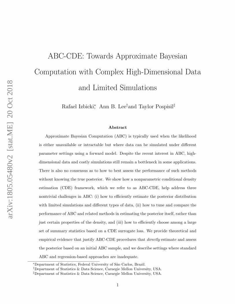
Theorem 3. Let F = f1, . . . , fm be a set of estimators of f(θ|xo). Assume that there

exists M such that |fi(θ|x)| ≤ M for every x, θ, and i = 1, . . . ,m.6 Moreover, assume that

for every θ ∈ Θ, gi,θ(x) := (fi(θ|x)− f(θ|x))2 satisfies the Holder condition of order β with

constants Kθ such that KH :=∫Kθdθ <∞. Then, for every ν > 0,

P(

maxf∈F|Lεxo(f , f) +Kf − Lxo(f , f)| ≥ Kεε

β + ν

)≤ 2me

− B′ν22(M2+2M)2 .

The next corollary shows that the procedure we propose in this section, with high proba-

bility, picks an estimate of the posterior density that has a true loss that is close to the true

loss of the best method in F .

Corollary 1. Let f ∗ := arg minf∈F Lεxo(f , f) be the best estimator in F according to the

estimated surrogate loss, and let f ∗ = arg minf∈F Lxo(f , f) be the best estimator in F ac-

cording to the true loss. Then, under the assumptions from Theorem 6, with probability at

least 1− 2me− B′ν2

2(M2+2M)2 , Lxo(f∗, f) ≤ Lxo(f

∗, f) + 2(KHεβ + ν).

2.3 Summary Statistics Selection

In a typical ABC setting, there are a large number of available summary statistics. Standard

ABC fails if all of them are used simultaneously, especially if some statistics carry little

information about the parameters of the model (Blum, 2010).

One can use ABC-CDE as a way of either (i) directly estimating f(θ|xo) when there

are a large number of summary statistics,7 or (ii) assigning an importance measure to each

summary statistic to guide variable selection in ABC and related procedures.

There are two versions of ABC-CDE that are particularly useful for variable selection:

6Such assumptions hold if the fi’s are obtained via FlexCode with bounded basis functions (e.g., Fourierbasis) or a kernel density estimator on the ABC samples.

7the dimension reduction is then implicit in the choice of (high-dimensional) regression method

13

FlexCode-SAM8 and FlexCode-RF9. Izbicki and Lee (2017) show that both estimators au-

tomatically adapt to the number of relevant covariates, i.e., the number of covariates that

influence the distribution of the response. In the context of ABC, this means that these

methods are able to automatically detect which summary statistics are relevant in estimat-

ing the posterior distribution of θ. Corollary 1 from Izbicki and Lee (2017) implies that, if

indeed only m out of all d summary statistics influence the distribution of θ, then the rate

of convergence of these methods is O(n−2β/(2β+m

2β+12α

+1))

instead of O(n−2β/(2β+d

2β+12α

+1))

,

where α and β are numbers associated to the smoothness of f(θ|x). The former rate implies

a much faster convergence: if m d, it is essentially the rate one would obtain if one

knew which were the relevant statistics. In such a setting, there is no need to explicitly

perform summary statistic selection prior to estimating the posterior; FlexCode-SAM or

FlexCode-RF automatically remove irrelevant covariates.

More generally, one can use FlexCode to compute an importance measure for summary

statistics (to be used in other procedures than FlexCode). It turns out that one can infer

the relevance of the j:th summary statistic in posterior estimation from its relevance in

estimating the I first regression functions in FlexCode — even if we do not use FlexCode

for estimating the posterior. More precisely, assume that x = (x1, . . . , xj, . . . , xd) is a vector

of summary statistics, and let x′j = (x1, . . . , xj−1, x′j, xj+1, . . . , xd). Define the relevance of

variable j to the posterior distribution f(θ|x) as

rj :=

∫ ∫ ∫(f(θ|x)− f(θ|x′j))2dxdx′jdθ,

and its relevance to the regression βi(x) in Equation 1 as

ri,j :=

∫ ∫ (βi(x)− βi(x′j)

)2dxdx′j.

8FlexCode with the coefficients from Equation 1 estimated via Sparse Additive Models (Ravikumar et al.,2009)

9FlexCode with the coefficients from Equation 1 estimated via Random Forests

14

Under some smoothness assumptions with respect to θ, the two metrics are related.

Assumption 1 (Smoothness in θ direction). ∀x∈X , we assume that f(θ|x)∈Wφ(sx, cx),

the Sobolev space of order s and radius c,10 where f(θ|x) is viewed as a function of θ, and

sx and cx are such that infx sxdef= β > 1

2and

∫c2xdx <∞.

Proposition 1. Under Assumption 2, rj =∑I

i=1 ri,j +O(I−2β

)Now let ui,j denote a measure of importance of the j:th summary statistic in estimating

regression i (Equation 1). For instance, for FlexCode-RF, ui,j may represent the mean

decrease in the Mean Squared Error (Hastie et al., 2001); for FlexCode-SAM, ui,j may

be value of the indicator function for the j:th summary statistic when estimating βi(x).

Motivated by Proposition 2, we define an importance measure for the j:th summary statistic

in posterior estimation according to

uj :=1

I

I∑i=1

ui,j. (6)

We can use these values to select variables for estimating f(θ|xo) via other ABC methods.

For example, one approach is to choose all summary statistics such that uj > t, where the

threshold value t is defined by the user. We will further explore this approach in Section 3.

In summary, our procedure has two main advantages compared to current state-of-the-

art approaches for selecting summary statistics in ABC: (i) it chooses statistics that lead

to good estimates of the entire posterior distribution f(θ|xo) rather than surrogates, such

as, the regression or posterior mean E[θ|xo] (Aeschbacher et al., 2012; Creel and Kristensen,

2016; Faisal et al., 2016), and (ii) it is typically faster than most other approaches; in

particular, it is significantly faster than best subset selection which scales as O(2d), whereas,

e.g., FlexCode-RF scales as O(Id), and FlexCode-SAM scales as O(Id3).

10For every s > 12 and 0 < c <∞, Wφ(s, c) := f =

∑i≥1 θiφi :

∑i≥1 a

2i θ

2i ≤ c2, where ai∼ (πi)s. Notice

that for the Fourier basis (φi)i, this is the standard definition of the Sobolev space of order s and radius c;it is the space of functions that have their s-th weak derivative bounded by c2 and integrable in L2.

15

3 Experiments

3.1 Examples with Known Posteriors

We start by analyzing examples with well-known and analytically computable posterior

distributions:

1. Mean of a Gaussian with known variance. X1, . . . , X20|µiid∼ Normal(µ, 1),

µ ∼ Normal(0, σ20). We repeat the experiments for σ0 in an equally spaced grid with

ten values between 0.5 and 100.

2. Precision of a Gaussian with unknown precision. X1, . . . , X20|(µ, τ)iid∼

Normal(µ, 1/τ), (µ, τ) ∼ Normal-Gamma(µ0, ν0, α0, β0). We set µ0 = 0, ν0 = 1, and

repeat the experiments choosing α0 and β0 such that E[τ ] = 1 and√V[τ ] is in an

equally spaced grid with ten values between 0.1 and 5.

In the Appendix we also investigate a third setting, “Mean of a Gaussian with unknown

precision”, with results similar to those shown here in the main manuscript.

In all examples here, observed data xo are drawn from a Normal(0, 1) distribution. We

run each experiment 200 times, that is, with 200 different values of xo. The training set T ,

which is used to build conditional density estimators, is constructed according to Algorithm

1 with B = 10, 000 and a tolerance level ε that corresponds to an acceptance rate of 1%. For

the distance function d(x,xo), we choose the Euclidean distance between minimal sufficient

statistics normalized to have mean zero and variance 1; these statistics are x for scenario 1

and (x, s) for scenario 2. We use a Fourier basis for all FlexCode experiments in the paper,

but wavelets lead to similar results.

We compare the following methods (see Section 4 and the appendix for a comparison

between ABC, regression adjustment methods and ABC-CDE with a standard kernel density

estimator):

• ABC: rejection ABC method with the minimal sufficient statistics (that is, apply a

kernel density estimator to the θ coordinate of T , with bandwidth chosen via cross-

16

validation),

• FlexCode Raw-NN: FlexCode estimator with Nearest Neighbors regression,

• FlexCode Raw-Series: FlexCode estimator with Spectral Series regression (Lee and

Izbicki, 2016), and

• FlexCode Raw-RF: FlexCode estimator with Random Forest regression.

The three FlexCode estimators (denoted by “Raw”) are directly applied to the sorted values

of the original covariates X(1), . . . , X(20). That is, we do not use minimal sufficient statistics

or other summary statistics. To assess the performance of each method, we compute the true

loss Lxo (Equation 2) for each xo. In addition, we estimate the surrogate loss Lεxo according

to Equation 5 using a new sample of size B′ = 10, 000 from Algorithm 1.

3.1.1 CDE and Method Selection

In this section, we investigate whether various ABC-CDE methods improve upon standard

ABC for the settings described above. We also evaluate the method selection approach in

Section 2.2 by comparing decisions based on estimated surrogate losses to those made if one

knew the true ISE losses.

Figure 3, left, shows how well the methods actually estimate the posterior density for

Settings 1-2. Panel (a) and (e) list the proportion of times each method returns the best

results (according to the true loss from Equation 2). Generally speaking, the larger the prior

variance, the better ABC-CDE methods perform compared to ABC. In particular, while for

small variances ABC tends to be better, for large prior variances, FlexCode with Nearest

Neighbors regression tends to give the best results. FlexCode with expansion coefficients

estimated via Spectral Series regression is also very competitive. Panels (c) and (g) confirms

these results; here we see the average true loss of each method along with standard errors.

Figure 3, right, summarizes the performance of our method selection algorithm. Panels

(b) and (f) list the proportion of times the method chosen by the true loss (Equation 2)

matches the method chosen via the estimated loss (Equation 5) in all pairwise comparisons;

17

that is, the plot tells us how often the method selection procedure proposed in Section

2.2 actually works. We present two variations of the algorithm: in the first version (see

triangles), we include all the data; in the second version (see circles), we remove cases where

the confidence interval for Lεxo(f1, f)− Lεxo(f2, f) contains zero (i.e., cases where we cannot

tell whether f1 or f2 performs better). The baseline shows what one would expect if the

method selection algorithm was totally random. The plots indicate that we, in all settings,

roughly arrive at the same conclusions with the estimated surrogate loss as we would if we

knew the true loss.

For the sake of illustration, we have also added panels (d) and (h), which show a scatter-

plot of differences between true losses versus the differences between the estimated losses for

ABC and FlexCode Raw-NN for the setting with σ0 = 0.5 and√V[τ ] = 0.1, respectively.

The fact that most samples are either in the first or third quadrant further confirms that the

estimated surrogate loss is in agreement with the true loss in terms of which method best

estimates the posterior density.

18

0%

25%

50%

75%

100%

0.50

11.5

622

.61

33.6

744

.72

55.7

866

.83

77.8

988

.94

100.

00

σ0

Bes

t met

hod

ABC FlexCode_Raw−NNFlexCode_Raw−RF FlexCode_Raw−Series

(a)

0%

25%

50%

75%

100%

0.5011

.5622

.6133

.6744

.7255

.7866

.8377

.8988

.94

100.

00

σ0

Agr

eem

ent b

etw

een

true

and

est

imat

ed l

oss

Without zeros All samples

(b)

0.01

0.10

0 25 50 75 100

σ0

Mea

n tr

ue lo

ss (

log

scal

e)


(c)

L(fABC,f)−L(fNN,f)

L ε^(f

AB

C,f)

−L ε^

(fN

N,f)

(d)

0%

25%

50%

75%

100%

0.10

0.64

1.19

1.73

2.28

2.82

3.37

3.91

4.46

5.00

V(τ)

Bes

t met

hod


(e)

0%

25%

50%

75%

100%

0.10

0.64

1.19

1.73

2.28

2.82

3.37

3.91

4.46

5.00

SD(τ)

Agr

eem

ent b

etw

een

true

and

est

imat

ed lo

ss


(f)

1e−02

2e−03

5e−03

0 1 2 3 4 5

V(τ)Mea

n tr

ue lo

ss (

log

scal

e)


(g)

L(fABC,f)−L(fNN,f)

L ε^(f

AB

C,f)

−L ε^

(fN

N,f)

(h)

Figure 3: Panels (a)-(d): CDE and method selection results for scenario 1 (mean of a Gaussian with knownvariance). Left: Panels (a) and (c) show that the rejection ABC leads to better estimates of the posteriordensity f(θ|xo) when the prior variance σ0 is small, but the NN and Series versions of FlexCode yield betterestimates for moderate and large values of σ0. Right: Panels (b) and (d) indicate that by estimating thesurrogate loss function one can tell from the data which method is better for the problem at hand. Thehorizontal line in panel (b) represents the behavior of a random selection. Panels (e)-(h): CDE and methodselection results for scenario 2 (precision of a Gaussian with unknown precision). Conclusions are analogous.

19

FlexCode−RF ABC

1 2 3 4 5 6 7 8 25 50 1 2 3 4 5 6 7 8 25 500.000

0.025

0.050

0.075

0.100

Number of Summary Statistics

Mea

n tr

ue lo

ss

σ00.5 11.56

22.61 33.67

(a)

0.0

0.1

0.2

0.3

0.4

Mea

n

Med

ian

Mea

n1

Mea

n2Sd

IQR

Quarti

le1

R1 R2 R3 R4 R5 R6 R7 R8 R9R10 R11 R12 R13 R14 R15 R16 R17 R18 R19 R20 R21 R22 R23 R24 R25 R26 R27 R28 R29 R30 R31 R32 R33 R34 R35 R36 R37 R38 R39 R40 R41 R42 R43

Summary Statistic

Ave

rage

Impo

rtan

ce Location Scale Random Noise

(b)

FlexCode−RF ABC

1 2 3 4 5 6 7 8 25 50 1 2 3 4 5 6 7 8 25 50

0.04

0.08

0.12

0.16


Mea

n tr

ue lo

ss

SD(τ)0.64 1.19

1.73 2.28

(c)

0.00.10.20.30.40.5

Mea

n

Med

ian

Mea

n1

Mea

n2Sd

IQR

Quarti

le1

R1 R2 R3 R4 R5 R6 R7 R8 R9R10 R11 R12 R13 R14 R15 R16 R17 R18 R19 R20 R21 R22 R23 R24 R25 R26 R27 R28 R29 R30 R31 R32 R33 R34 R35 R36 R37 R38 R39 R40 R41 R42 R43

Summary Statistic

Ave

rage

Impo

rtan

ce Location Scale Random Noise

(d)

Figure 4: Panels (a)-(b): Summary statistic selection for scenario 1 (mean of a Gaussian with knownvariance); Panels (c)-(d): Summary statistic selection for scenario 2 (precision of a Gaussian with unknownprecision). Panels (a) and (c) show that ABC is highly sensitive to random noise (entries 8-51) with theestimates of the posteriors rapidly deteriorating with nuisance statistics. Nuisance statistics do not affectthe performance of FlexCode-RF much. Furthermore, we see from panel (b) that FlexCode-RF identifiesthe location statistics (entries 1-5) as key variables for the first setting and assigns them a high averageimportance score. In the second setting, panel (d) indicates that we only need dispersion statistics (such asentry 5) to estimate the posteriors wells.

20

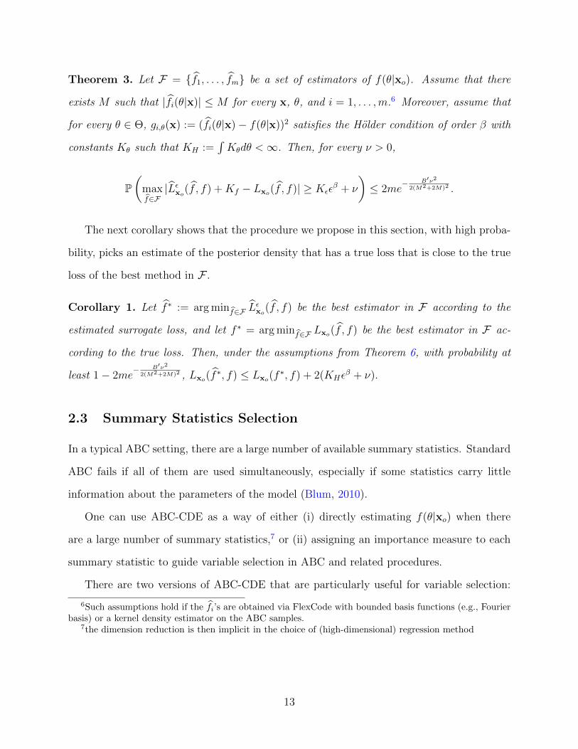
3.1.2 Summary Statistic Selection

In this Section we investigate the performance of FlexCode-RF for summary statistics selec-

tion (Sec. 2.3). For this purpose, the following summary statistics were used:

1. Mean: average of the data points; 1n

∑ni=1Xi

2. Median: median of the data points; medianXii=1,...,n

3. Mean 1: average of the first half of the data points; 1n/2

∑n/2i=1Xi

4. Mean 2: average of the second half of the data points; n/2+1n

∑ni=n/2+1Xi

5. SD: standard deviation of the data points;√

1n

∑ni=1(Xi − X)2

6. IQR: interquartile range of the data points; quantile75%Xii=1,...,n−quantile25%Xii=1,...,n

7. Quartile 1: first quantile of the data points; quantile25%Xii=1,...,n

8–51. Independent random variables ∼ Normal(0, 1), that is, random noise

Figure 4 summarizes the results of fitting FlexCode-RF and ABC to these summary

statistics for the different scenarios. Panel (a) and (c) show the true loss as we increase the

number of statistics. More precisely: the values at x = 1 represent the true loss of ABC

(left) and FlexCode-RF (right) when using only the mean (i.e., the first statistic); the points

at x = 2 indicate the true loss of the estimates using only the mean and the median (i.e.,

the first and second statistics) and so on. We note that FlexCode-RF is robust to irrelevant

summary statistics: the method virtually behaves as if they were not present. This is in sharp

contrast with standard ABC, whose performance deteriorates quickly with added noise or

nuisance statistics.

Furthermore, panels (b) and (d) show the average importance of each statistic, defined

according to Equation 6, where ui,j is the mean decrease in the Gini index. These plots

reveal that FlexCode-RF typically assigns a high score to sufficient summary statistics or

to statistics that are highly correlated to sufficient statistics. For instance, in panel (b)

(estimation of the mean of the distribution), measures of location are assigned a higher

importance score, whereas measures of dispersion are assigned a higher score in panel (d)

21

(estimation of the precision of the distribution). In all examples, FlexCode-RF assigns zero

importance to random noise statistics. We conclude that our method for summary statistic

selection indeed identifies relevant statistics for estimating the posterior f(θ|xo) well.

4 Approximate Bayesian Computation and Beyond

In this section, we show how one can use our surrogate loss to choose the tuning parameters

in standard ABC with a nearest neighbors kernel smoother.

4.1 ABC with Fewer Simulations

As noted by (Blum, 2010; Biau et al., 2015), ABC is equivalent to a kernel-CDE. More

specifically, it can be seen as a “nearest-neighbors” kernel-CDE (NN-KCDE) defined by

fnn(θ | x) =1

k

k∑i=1

Kh(ρ(θ, θsi(x))), (7)

where si(x) represents the index of the ith nearest neighbor to the target point x in covariate

space, and we compute the conditional density of θ at x by applying a kernel smoother Kh(·)

with bandwidth h to the k points closest to x.

For a given set of generated data, the above is equivalent to selecting the ABC threshold

ε as the k/n-th quantile of the observed distances. This is commonly used in practice as it is

more convenient than determining ε a priori. However, as pointed out by Biau et al. (2015)

(Section 4; remark 1), there is currently no good methodology to select both k and h in an

ABC k-nearest neighbor estimate.

Given the connection between ABC and NN-KCDE, we propose to use our surrogate loss

to tune the estimator; selecting k and h such that they minimize the estimated surrogate

loss in Equation 5. In this sense, we are selecting the “optimal” ABC parameters after

generating some of the data: having generated 10,000 points, it may turn out that we would

22

have preferred a smaller tolerance level ε and that only using the closest 1,000 points would

better approximate the posterior.

Example with Normal Posterior. To demonstrate the effectiveness of our surrogate

loss in reducing the number of simulations, we draw data X1, . . . , X5|µiid∼ Normal(µ, 0.22)

where µ ∼ Normal(1, 0.52). We examine the role of ABC thresholds by fitting the model

for several values of the threshold with observed data x0 = −0.5,−0.25, 0.0, 0.25, 0.5. (A

similar example with a two-dimensional normal distribution can be found in the Appendix.)

For each threshold, we perform rejection sampling until we retain B = 1000 ABC points. We

select ABC thresholds to fix the acceptance rate of the rejection sampling. Those acceptance

rates are then used in place of the actual tolerance level ε for easier comparison.

0.01 0.5 1

AB

CN

N−

KC

DE

FlexC

ode−N

N

−2 0 2 −2 0 2 −2 0 2

0.00

0.25

0.50

0.75

0.00

0.25

0.50

0.75

0.00

0.25

0.50

0.75

θ

p(θ|

x)

ISE Surrogate + Constant

0.01 0.25 0.5 0.75 1 0.01 0.25 0.5 0.75 1

0

1

2

3

Acceptance Rate

Loss

Method ABC NN−KCDE FlexCode−NN

Normal Posterior

Figure 5: Left: Density estimates for normal posterior using ABC sample of varying acceptance rates (0.01,0.5, and 1). As the acceptance rate (or, equivalently, the ABC tolerance level) decreases, the ABC posteriorapproaches the true posterior. Both NN-KCDE and FlexCode-NN approximate the posterior well for allacceptance rates, even for an acceptance rate of 1 which corresponds to no ABC threshold. Right: Trueintegrated squared error (ISE) loss and estimated surrogate loss for normal posterior using ABC sample ofvarying acceptance rates. We need to decrease the acceptance rate considerably to attain a small loss forABC. On the other hand, the losses for NN-KCDE and FlexCode-NN are small for all thresholds.

The left panel of Figure 5 shows examples of posterior densities for varying acceptance

rates. For the highest acceptance rate of 1 (corresponding to the ABC tolerance level ε→∞),

23

the ABC posterior (top left) is the prior distribution and thus a poor estimate. In contrast,

the two ABC-CDE methods (FlexCode-NN and NN-KCDE) have a decent performance even

at an acceptance rate of 1; more generally, they perform well at a higher acceptance rate

than standard ABC.

To corroborate this qualitative look, we examine the loss for each method. The right

panel of Figure 5 plots the true and surrogate losses against the acceptance rate for the

given methods. As seen in Section 3.1.1, the surrogate loss provides the same conclusion as

the (unavailable in practice) true loss. As the acceptance rate decreases, the ABC realizations

more closely approximate the true posterior and the ABC estimate of the posterior improves.

The main result is that NN-KCDE and FlexCode-NN have roughly constant performance

over all values of the acceptance rate. As such, we could generate only 1,000 realizations

of the ABC sample at an acceptance rate of 1 and achieve similar result as standard ABC

generating 100,000 values at an acceptance rate of 0.01.

There are two different sources of improvement: the first exhibited by NN-KCDE amounts

to selecting the “optimal” ABC parameters k and h using surrogate loss. However, as

FlexCode-NN performs slightly better than NN-KCDE for the same sample, there is an

additional improvement in using CDE methods other than kernel smoothers; this difference

becomes more pronounced for high-dimensional and complex data (see Izbicki and Lee 2017

for examples of when traditional kernel smoothers fail).

5 Conclusions

In this work, we have demonstrated three ways in which our conditional estimation frame-

work can improve upon approximate Bayesian computational methods for next-generation

complex data and simulations.

First, realistic simulation models are often such that the computational cost of generating

a single sample is large, making lower acceptance ratios unrealistic.

24

Secondly, our ABC-CDE framework allows one to compare ABC and related methods in

a principled way, making it possible to pick the best method for a given data set without

knowing the true posterior. Our approach is based on a surrogate loss function and data

splitting. We note that a related cross-validation procedure to choose the tolerance level

ε in ABC has been proposed by Csillery et al. (2012), albeit using a loss function that is

appropriate for point estimation only.

Finally, when dealing with complex models, it is often difficult to know exactly what

summary statistics would be appropriate for ABC. Nevertheless, the practitioner can usu-

ally make up a list of a large but redundant number of candidate statistics, including statis-

tics generated with automatic methods. As our results show, FlexCode-RF (unlike ABC)

is robust to irrelevant statistics. Moreover, FlexCode, in combination with RF for regres-

sion, offers a way of evaluating the importance of each summary statistic in estimating the

full posterior distribution; hence, these importance scores could be used to choose relevant

summary statistics for ABC and any other method used to estimate posteriors.

In brief, there are really two estimation problems in ABC-CDE: The first is that of

estimating f(θ|xo). ABC-CDE starts with a rough approximation from an ABC sampler

and then directly estimates the conditional density exactly at the point x = xo using a

nonparametric conditional density estimator. The second is that of estimating the integrated

squared error loss (Eq. 2). Here we propose a surrogate loss that weights all points in the

ABC posterior sample equally, but a weighted surrogate loss could potentially return more

accurate estimates of the ISE. For example, Figures 9 (left) and 10 in the Appendix show that

NN-KCDE perform better than ABC post-processing techniques. The current estimated loss,

however, cannot identify a difference in ISE loss between NN-KCDE and “Blum” because of

the rapidly shifting posterior in the vicinity of x = x0.

Acknowledgments. We are grateful to Rafael Stern for his insightful comments on the manuscript.

We would also like to thank Terrence Liu, Brendan McVeigh, and Matt Walker for the NFW simu-

25

lation code and to Michael Vespe for help with the weak lensing simulations in the Appendix. This

work was partially supported by NSF DMS-1520786, Fundacao de Amparo a Pesquisa do Estado

de Sao Paulo (2017/03363-8) and CNPq (306943/2017-4).

Links to Nonparametric Software Optimized for CDE:

• FlexCode: https://github.com/rizbicki/FlexCoDE; https://github.com/tpospisi/flexcode

• NN-KCDE: https://github.com/tpospisi/NNKCDE (see Appendix D)

• RF-CDE: https://github.com/tpospisi/rfcde (Pospisil and Lee, 2018)

References

Abbott, T., F. B. Abdalla, S. Allam, et al. (2016, July). Cosmology from cosmic shear with Dark Energy

Survey Science Verification data. Physical Review D 94 (2), 022001.

Aeschbacher, S., M. A. Beaumont, and A. Futschik (2012). A novel approach for choosing summary statistics

in approximate Bayesian c omputation. Genetics 192 (3), 1027–1047.

Beaumont, M. A. (2010). Approximate bayesian computation in evolution and ecology. Annual Review of

Ecology, Evolution, and Systematics 41, 379–406.

Beaumont, M. A., J. Cornuet, J. Marin, and C. P. Robert (2009). Adaptive approximate bayesian compu-

tation. Biometrika, asp052.

Beaumont, M. A., W. Zhang, and D. J. Balding (2002). Approximate bayesian computation in population

genetics. Genetics 162 (4), 2025–2035.

Biau, G., F. Cerou, and A. Guyader (2015). New insights into approximate bayesian computation. In

Annales de l’Institut Henri Poincare, Probabilites et Statistiques, Volume 51, pp. 376–403. Institut Henri

Poincare.

Bickel, P. J., Y. Ritov, and T. M. Stoker (2006). Tailor-made tests for goodness of fit to semiparametric

hypotheses. The Annals of Statistics, 721–741.

Blum, M. G. (2010). Approximate bayesian computation: a nonparametric perspective. Journal of the

American Statistical Association 105 (491), 1178–1187.

26

https://github.com/rizbicki/FlexCoDE

https://github.com/tpospisi/flexcode

https://github.com/tpospisi/NNKCDE

https://github.com/tpospisi/rfcde

Blum, M. G. B. and O. Francois (2010). Non-linear regression models for approximate bayesian computation.

Statistics and Computing 20 (1), 63–73.

Blum, M. G. B., M. A. Nunes, D. Prangle, and S. A. Sisson (2013). A comparative review of dimension

reduction methods in approximate bayesian computation. Statistical Science 28 (2), 189–208.

Breiman, L. (2001). Statistical modeling: The two cultures. Statistical Science 16 (3), 199–231.

Cameron, E. and A. Pettitt (2012). Approximate bayesian computation for astronomical model analysis: a

case study in galaxy demographics and morphological transformation at high redshift. Monthly Notices

of the Royal Astronomical Society 425 (1), 44–65.

Chen, T. and C. Guestrin (2016). Xgboost: A scalable tree boosting system. In Proceedings of the 22nd acm

sigkdd international conference on knowledge discovery and data mining, pp. 785–794. ACM.

Creel, M. and D. Kristensen (2016). On selection of statistics for approximate bayesian computing (or the

method of simulated moments). Computational Statistics & Data Analysis 100, 99–114.

Csillery, K., O. Francois, and M. G. B. Blum (2012). abc: an r package for approximate bayesian computation

(abc). Methods in Ecology and Evolution.

Estoup, A., E. Lombaert, J. Marin, et al. (2012). Estimation of demo-genetic model probabilities with

approximate bayesian computation using linear discriminant analysis on summary statistics. Molecular

Ecology Resources 12 (5), 846–855.

Faisal, M., A. Futschik, I. Hussain, and M. Abd-el. Moemen (2016). Choosing summary statistics by least

angle regression for approximate bayesian computation. Journal of Applied Statistics, 1–12.

Fan, Y., D. J. Nott, and S. A. Sisson (2013). Approximate bayesian computation via regression density

estimation. Stat 2 (1), 34–48.

Fearnhead, P. and D. Prangle (2012). Constructing summary statistics for approximate bayesian computa-

tion: semi-automatic approximate bayesian computation. Journal of the Royal Statistical Society: Series

B (Statistical Methodology) 74 (3), 419–474.

Ferraty, F. and P. Vieu (2006). Nonparametric functional data analysis: theory and practice. Springer Science

& Business Media.

27

Harnois-Deraps, J. and L. van Waerbeke (2015, July). Simulations of weak gravitational lensing - II. Including

finite support effects in cosmic shear covariance matrices. Monthly Notices of the Royal Astronomical

Society 450, 2857–2873.

Hastie, T., R. Tibshirani, and J. H. Friedman (2001). The elements of statistical learning: data mining,

inference, and prediction. New York: Springer-Verlag.

Hildebrandt, H., M. Viola, C. Heymans, et al. (2017, February). KiDS-450: cosmological parameter con-

straints from tomographic weak gravitational lensing. Monthly Notices of the Royal Astronomical Soci-

ety 465, 1454–1498.

Hoekstra, H. and B. Jain (2008). Weak gravitational lensing and its cosmological applications. Annual

Review of Nuclear and Particle Science 58, 99–123.

Izbicki, R. and A. Lee (2017). Converting high-dimensional regression to high-dimensional conditional density

estimation. Eletronic Journal of Statistics 11, 2800–2831.

Lee, A. B. and R. Izbicki (2016). A spectral series approach to high-dimensional nonparametric regression.

Electronic Journal of Statistics 10 (1), 423–463.

Li, J., D. J. Nott, Y. Fan, and S. A. Sisson (2015). Extending approximate bayesian computation methods

to high dimensions via gaussian copula. arXiv preprint arXiv:1504.04093 .

Li, W. and P. Fearnhead (2017). Convergence of regression adjusted approximate bayesian computation.

Biometrika.

Liddle, A. (2015). An introduction to modern cosmology. John Wiley & Sons.

Liu, T. and M. Walker (2018). In preparation.

Lueckmann, J. M., P. J. Goncalves, G. Bassetto, et al. (2017). Flexible statistical inference for mechanistic

models of neural dynamics. In Advances in Neural Information Processing Systems, pp. 1289–1299.

Mallat, S. (1999). A wavelet tour of signal processing. Academic press.

Mandelbaum, R. (2017). Weak lensing for precision cosmology. arXiv preprint:1710.03235 .

Marin, J. M., P. Pudlo, C. P. Robert, and R. J. Ryder (2012). Approximate Bayesian computational methods.


28

Munshi, D., P. Valageas, L. Van Waerbeke, and A. Heavens (2008). Cosmology with weak lensing surveys.

Physics Reports 462 (3), 67–121.

Navarro, J. F. (1996). The structure of cold dark matter halos. In Symposium-international astronomical

union, Volume 171, pp. 255–258. Cambridge University Press.

Papamakarios, G. and I. Murray (2016). Fast ε-free inference of simulation models with bayesian conditional

density estimation. arXiv preprint arXiv:1605.06376 .

Petri, A. (2016). Mocking the weak lensing universe: The lenstools python computing package. Astronomy

and Computing 17, 73–79.

Pospisil, T. and A. B. Lee (2018). RFCDE: Random forests for conditional density estimation. arXiv

preprint:1804.05753 .

Prangle, D., M. G. B. Blum, G. Popovic, and S. A. Sisson (2014). Diagnostic tools for approximate bayesian

computation using the coverage property. Australian & New Zealand Journal of Statistics 56 (4), 309–329.

R Core Team (2013). R: A Language and Environment for Statistical Computing. Vienna, Austria: R

Foundation for Statistical Computing. ISBN 3-900051-07-0.

Ravikumar, P., J. Lafferty, H. Liu, and L. Wasserman (2009). Sparse additive models. Journal of the Royal

Statistical Society, Series B 71 (5), 1009–1030.

Raynal, L., J.-M. Marin, , et al. (2017). ABC random forests for Bayesian parameter inference. arXiv

preprint arXiv:1605.05537 .

Rowe, B., M. Jarvis, R. Mandelbaum, et al. (2015). Galsim: The modular galaxy image simulation toolkit.

Astronomy and Computing 10, 121–150.

Sato, M., M. Takada, T. Hamana, and T. Matsubara (2011, June). Simulations of Wide-field Weak-lensing

Surveys. II. Covariance Matrix of Real-space Correlation Functions. The Astrophysical Journal 734, 76.

Sisson, S. A., Y. Fan, and M. M. Tanaka (2007). Sequential Monte Carlo without likelihoods. Proceedings

of the National Academy of Sciences 104 (6), 1760–1765.

Strigari, L. E., C. S. Frenk, and S. D. M. White (2017). Dynamical models for the Sculptor dwarf spheroidal

in a λCDM universe. The Astrophysical Journal 838 (2), 123.

29

Weyant, A., C. Schafer, and W. M. Wood-Vasey (2013). Likelihood-free cosmological inference with type ia

supernovae: Approximate bayesian computation for a complete treatment of uncertainty. The Astrophys-

ical Journal 764 (2), 116.

30

A Proofs

A.1 Results on the surrogate loss

Theorem 4. Assume that, for every θ ∈ Θ, gθ(x) := (f(θ|x) − f(θ|x))2 satisfies the Holder

condition of order β with a constant Kθ11 such that KH :=

∫Kθdθ <∞. Then

|Lεxo(f , f)− Lxo(f , f)| = KHεβ = O(εβ)

Proof. First, notice that

Lxo(f , f) =

∫gθ(xo)dθ

∫f(x)I(d(x,xo) < ε)

P(d(X,xo) < ε)dx =

∫ ∫gθ(xo)

f(x)I(d(x,xo) < ε)

P(d(X,xo) < ε)dxdθ.

It follows that

|Lεxo(f , f)− Lxo(f , f)| =∣∣∣∣∫ (∫ gθ(x)

f(x)I(d(x,xo) < ε)

P(d(X,xo) < ε)dx−

∫gθ(xo)

f(x)I(d(x,xo) < ε)

P(d(X,xo) < ε)dx

)dθ

∣∣∣∣=

∣∣∣∣∫ (∫ (gθ(x)− gθ(xo))f(x)I(d(x,xo) < ε)

P(d(X,xo) < ε)dx

)dθ

∣∣∣∣≤∫ (∫

|gθ(x)− gθ(xo)|f(x)I(d(x,xo) < ε)

P(d(X,xo) < ε)dx

)dθ

≤∫ (∫

Kθd(x,xo)β f(x)I(d(x,xo) < ε)

P(d(X,xo) < ε)dx

)dθ

≤∫Kθε

β

(∫f(x)I(d(x,xo) < ε)

P(d(X,xo) < ε)dx

)dθ

= εβ∫Kθ1dθ = KHε

β

11That is, there exists a constant Kθ such that for every x,y ∈ <d |gθ(x)− gθ(y)| ≤ Kθ(d(x,y))β .

31

Proof. Notice that

|Lεxo(f , f) +Kf − Lxo(f , f)| −KHεβ

= |Lεxo(f , f) +Kf − Lεxo(f , f) + Lεxo(f , f)− Lxo(f , f)| −KHεβ

≤ |Lεxo(f , f) +Kf − Lεxo(f , f)|+ |Lεxo(f , f)− Lxo(f , f)| −KHεβ

≤ |Lεxo(f , f) +Kf − Lεxo(f , f)|,

where the last line follows from Theorem 4. It follows that

|Lεxo(f , f) +Kf − Lxo(f , f)| ≥ KHεβ + ν ⇒ |Lεxo(f , f) +Kf − Lεxo(f , f)| ≥ ν.

The conclusion follows from Lemma 1.

Theorem 6. Let F = f1, . . . , fm be a set of estimators of f(θ|xo). Assume there exists M such

that |fi(θ|x)| ≤ M for every x, θ, and i = 1, . . . ,m. 12 Moroever, assume that for every θ ∈ Θ,

gi,θ(x) := (fi(θ|x)− f(θ|x))2 satisfies the Holder condition of order β with constants Kθ such that

KH :=∫Kθdθ <∞. Then,

P

(maxf∈F|Lεxo(f , f) +Kf − Lxo(f , f)| ≥ Kεε

β + ν

)≤ 2me

− B′ν22(M2+2M)2 .

Proof. The theorem follows from Lemma 2 and the union bound.

Corollary 2. Let f∗ := arg minf∈F L

εxo(f , f) be the best estimator in F according to the estimated

surrogate loss, and let f∗ = arg minf∈F Lxo(f , f) be the best estimator in F according to the true

loss. Then, under the assumptions from Theorem 6, with probability at least 1− 2me− B′ν2

2(M2+2M)2 ,

Lxo(f∗, f) ≤ Lxo(f

∗, f) + 2(KHεβ + ν).

12Such assumptions hold if the fi’s are obtained via FlexCode with bounded basis functions (e.g., Fourierbasis) or a kernel density estimator on the ABC samples.

33

Proof. From Theorem 6, with probability at least 1− 2me− B′ν2

2(M2+2M)2

Lxo(f∗, f)−Lxo(f

∗, f) =

Lxo(f∗, f)− (Lεxo(f

∗, f) +Kf )

+ (Lεxo(f∗, f) +Kf )− (Lεxo(f

∗, f) +Kf )

+ (Lεxo(f∗, f) +Kf )− Lxo(f

∗, f)

≤ 2(KHεβ + ν),

where the inequality follows from the fact that, by definition, (Lεxo(f∗, f)+Kf )−(Lεxo(f

∗, f)+Kf ) <

0 and Lxo(f , f)− (Lεxo(f , f) +Kf ) ≤ KHεβ + ν for every f ∈ F .

A.2 Results on summary statistics selection

Assumption 2 (Smoothness in θ direction). ∀x∈X , f(θ|x)∈Wφ(sx, cx), where f(θ|x) is viewed

as a function of θ, and sx and cx are such that infx sxdef= β > 1

2 and∫c2xdx <∞.

Lemma 3. Let x = (x1, . . . , xd) and x′ = (x1, . . . , x′j , . . . , xd). Then, for every x and xj, gx,xj (θ) :=

f(θ|x)− f(θ|x′j) ∈Wφ(β, c2x + c2x′j

+ 2√c2xc

2x′j).

Proof. First we expand f(θ|x) and f(θ|x′j) in the basis (φi)i. We have that

gx,xj (θ) = f(θ|x)− f(θ|x′j) =∑i≥0

(βi(x)− βi(x′j))φi(θ).

34

Now, using Cauchy-Schwarz inequality, the expansion coefficients satisfy

∑i≥1

i2β(βi(x)− βi(x′j))2

=∑i≥1

i2β(βi(x))2 +∑i≥1

i2β(βi(x′j))

2 + 2∑i≥1

i2ββi(x)βi(x′j)

≤ c2x + c2x′j

+ 2

√√√√√∑i≥1

i2β(βi(x))2

∑i≥1

i2β(βi(x′j))2

≤ c2x + c2x′

j+ 2√c2xc

2x′j,

where the last inequality follows from Assumption 2.

Proposition 2. Under Assumption 2,

rj =

I∑i=1

ri,j +O(I−2β

)

Proof. Because βi(x)− βi(x′j) are the expansion coefficients of f(θ|x)− f(θ|x′j) on the basis (φi)i,

it follows from Lemma 3 (see appendix) that

∑i≥I

I2β(βi(x)− βi(x′j)

)2 ≤∑i≥I

i2β(βi(x)− βi(x′j)

)2 ≤ c2x + c2x′j

+ 2√c2xc

2x′j.

Hence,

∑i≥I

ri,j =∑i≥I

∫ ∫ (βi(x)− βi(x′j)

)2dxdx′j ≤

K

I2β= O(I−2β). (9)

Because f(θ|x)− f(θ|x′j) =∑

i≥0(βi(x)− βi(x′j))φi(θ) and the basis (φi)i is orthonormal, we have

that

rj =

∫ ∫ ∑i≥0

(βi(x)− βi(x′j))2dxdx′j =∑i≥0

ri,j . (10)

35

The final result follows from putting Equations 9 and 10 together.

B Mean of a Gaussian with unknown precision

In this section, we repeat the experiments of Section 3.1 of the paper, but in the caseX1, . . . , X20|(µ, τ)iid∼

N(µ, 1/τ), (µ, τ) ∼ Normal-Gamma(µ0, ν0, α0, β0). We set µ0 = 0, α0 = 2, β0 = 50 and repeat the

experiments for ν0 in an equally spaced grid with ten values between 0.001 and 1.

0%

25%

50%

75%

100%

0.00

10.

112

0.22

30.

334

0.44

50.

556

0.66

70.

778

0.88

91.

000

ν0

Bes

t met

hod


(a)

0%

25%

50%

75%

100%

0.00

0.11

0.22

0.33

0.44

0.56

0.67

0.78

0.89

1.00

ν0A

gree

men

t bet

wee

n tr

ue a

nd e

stim

ated

loss


(b)

1e−02

2e−02

4e−02

0.00

0.25

0.50

0.75

1.00

ν0

Mea

n tr

ue lo

ss (

log

scal

e)


(c)

−0.04 −0.02 0.00 0.02 0.04

−0.

15−

0.10

−0.

050.

000.

050.

100.

15

True loss ABC − True loss FlexCode_Raw_NN

Est

imat

ed lo

ss A

BC

− E

stim

ated

loss

Fle

xCod

e_R

aw_N

N

(d)

Figure 6: CDE and method selection results for scenario 3 (mean of a Gaussian with unknown precision).Left: Panels (a) and (c) show that the NN version of FlexCode yield better estimates of the posterior densityf(θ|xo) than the competing methods. Right: Panels (b) and (d) indicate that one by estimating the surrogateloss function can tell from the data which method is better for the problem at hand. The horizontal line inpanel (b) represents the behavior of a random selection.

36

ABC FlexCode−RF

1 2 3 4 5 6 7 8 25 50 1 2 3 4 5 6 7 8 25 500.01

0.02

0.03

0.04


Mea

n tr

ue lo

ssν0

0.22 0.330.44 0.56

(a)

0.00

0.05

0.10

0.15

Mea

n

Med

ian

Mea

n1

Mea

n2

Quarti

le1

SdIQ

R R1 R2 R3 R4 R5 R6 R7 R8 R9R10 R11 R12 R13 R14 R15 R16 R17 R18 R19 R20 R21 R22 R23 R24 R25 R26 R27 R28 R29 R30 R31 R32 R33 R34 R35 R36 R37 R38 R39 R40 R41 R42 R43

Summary Statistic

Ave

rage

Impo

rtan

ce

Location Scale Random Noise

(b)

Figure 7: Summary statistic selection for scenario 3 (mean of a Gaussian with unknown precision). Panel(a) shows the performance of ABC and FlexCode-RF using different sets of summary statistics. The ABCestimates of the posteriors rapidly deteriorate when adding other statistics than the location statistics 1-5(top left), whereas nuisance statistics do not decrease the performance of FlexCode-RF significantly (topright). Panel (b), furthermore, shows that FlexCode-RF identifies the location statistics (entries 1-5) as keyvariables and assigns them a high average importance score.

C Application I: Estimating a Galaxy’s Dark Matter

Density Profile

Next we consider more complex simulations. The ΛCDM (Lambda cold dark matter) model is

frequently referred to as the standard model of Big Bang cosmology (Liddle, 2015); it is the simplest

model that contains assumptions consistent with observational and theoretical knowledge of the

Universe.

37

The ΛCDM model predicts that the dark matter profile of a galaxy in the absence of baryonic

effects can be parameterized by the Navarro-French-White (NFW) model (Navarro, 1996). Given an

observed galaxy, such as the Sculptor dwarf spheroidal galaxy, we wish to constrain the parameters

of the NFW model. To begin we will only consider a single parameter, the critical energy Ec

(Strigari et al. 2017, Equation 15), and set all other parameters at commonly accepted estimates;

see Section C.1 for details.

The observed data x0 are velocities and coordinates of 200 stars in a galaxy, here simulated

so as to follow the NFW model.13 To perform ABC we define the distance function as the `2

norm between bivariate kernel density estimates of the joint distribution of the velocity and dis-

tance from the center. The same distance function will be used by FlexCode-NN and FlexCode-

Series. Because the data are functional we also implement a third version of ABC-CDE based

on FlexCode-Functional, where the coefficients in FlexCode are estimated via functional kernel

regression (Ferraty and Vieu, 2006).

To assess the performance of the CDE methods we generate 1000 test observations each with

an ABC sample of 1000 accepted observations with an acceptance rate of 0.1. We use the prior

Ec ∼ U(0.01, 1.0).

Analytic Estimated

0.00 0.25 0.50 0.75 1.00 0.00 0.25 0.50 0.75 1.00

0

20

40

60

Ec

Loss

ABC FlexCode−Functional FlexCode−NN FlexCode−Series

Figure 8: Left: True loss for each method in different parameter regions. Right: The estimated surrogateloss (here shifted with a constant

∫f(θ|xo)2dθ for easier comparison) can be used to identify when our

methods improve upon the ABC estimates.

Figure 8, left, displays the true loss for each method. The plot indicates that, for at least

some realizations with low true Ec, the estimates from the FlexCode estimators lead to better

13The simulations are written by Mao-Shen (Terrence) Liu and rely on an MCMC sampling scheme; thedetails are outlined in Liu and Walker 2018.

38

performance than ABC. Of most interest is that we reach similar conclusions with the estimated

surrogate loss; see right plot. Thus the surrogate loss serves as a reasonable proxy for the true loss

which in practical applications will be unavailable.

C.1 Additional details

Under the NFW model the joint likelihood for the specific angular momentum J and specific energy

E factorizes independently

f(E, J) ∝ g(J)h(E) (11)

with

g(J) =

[1 + (J/Jβ)−b]−1 b ≤ 0

1 + (J/Jβ)b b > 0

(12)

and

h(E) =

Eα(Eq + Eqc )d/q(Φlim − E)e E < Φlim

0 E ≥ Φlim

(13)

We can relate E and J to the observed values of position r and velocity v as follows

E =1

2v2 + Φs(1−

log(1 + rrs

)rrs

)

J = vr sin(θ)

We set the following constants at commonly accepted values in Table 1 and focus only on

estimating Ec.

Figure 9 displays examples of estimated posterior; each plot consists of an observed sample

generated using a different true of Ec.

39

Table 1: Parameter values used for the simulations of the Galaxy’s Dark Matter DensityProfile Model as reported by Strigari et al. (2017).

Parameter Valueα 2.0d -5.3e 2.5vmax 21rmax 1.5φs (vmax/0.465)2

rs rmax/2.16rlim 1.5

φlim φs(1−log(1+

rlimrs

)rlimrs

b -9.0q 6.9Jβ 0.086

0

10

20

30

0

10

20

30

0

10

20

30

0

10

20

30

AB

CF

lexCode−

Functional

FlexC

ode−N

NF

lexCode−

Series

0.2 0.4 0.6 0.8 1.0 0.2 0.4 0.6 0.8 1.0 0.2 0.4 0.6 0.8 1.0 0.2 0.4 0.6 0.8 1.0EC

P(E

C |

X)

Figure 9: Sample posterior densities for simulated galaxy data; the dashed curve is the true posterior, andthe vertical line indicates the true parameter value.

40

D Fast Implementation of NN-KCDE

NN-KCDE (or nearest-neighbors kernel CDE) is the usual kernel density estimate using only the

points closest in covariate space to the target point x:

fnn(θ | x) =1

k

k∑i=1

Kh(ρ(θ, θsi(x))), (14)

where si(x) represents the index of the ith nearest neighbor to x. As mentioned in Section 4.1,

NN-KCDE has a close connection with ABC in that, for every choice of k for a data set, there

is a choice of ε for the accept-reject ABC algorithm that produces an equivalent estimate of the

posterior. With the CDE loss, we can choose k to minimize the loss and improve upon the naive

pre-selected ε approach. For large ε we expect k to be small to avoid bias in the posterior estimate.

As ε shrinks, larger values of k will be selected to reduce the variance of the estimate.

To make this model selection procedure computationally feasible, we need to be able to effi-

ciently calculate the surrogate loss function. We examine the two terms (Section 2.2, Equation 5)

separately: The second term ∑i

f(θi | xi)

poses no difficulties as we simply plug in the kernel density estimate. The first term

∑i

∫f2(θ | xi)dz

is more difficult. Numerically integrating this integral is infeasible especially as the number of

validation samples increases.

Fortunately there is an analytic solution. We can express the integral in terms of convolutions

of the kernel function:

∫f2(θ | x)dz =

1

k2h

∑i∈Nk(x)

∑j∈Nk(x)

∫K(t)K

(t− di,j

h

)dt

with di,j representing the pairwise distance between points xi and xj . In the Gaussian case we

41

have the analytic solution

∫K(t)K(t− d)dt =

1

2√π

exp

(−d2

4

)

For other kernels we can work out the analytic solution as well, or, if that proves intractable,

we can approximate the function using numerical integration.

For both terms we have nested calculations, in that we can reuse computations for k = k1 < k2

when calculating the estimated loss for k = k2. In this way, there is little additional computational

time in considering all settings for k as opposed to trying only a large value of k.

An implementation of this method is available at https://github.com/tpospisi/NNKCDE.

E Two-Dimensional Normal.

We can extend the normal example of Section 4 of the paper to multiple dimensions with similar

results. Given a two-dimensional multivariate normal with fixed covariance ΣX = I2, we put a

normal conjugate prior on the mean µ ∼ N(µ0 = 0,Σ0 = I2). This results in the true posterior

µ | X ∼ N(µn,Σn),

where

µn = Σ0(Σ0 +1

nΣX)−1x+

1

nΣX(Σ0 +

1

nΣX)−1µ0

Σn =1

nΣ0(Σ0 +

1

nΣX)−1ΣX

As before we use the sufficient statistic of the sample mean as our statistic and the Euclidean norm

as the distance function.

Figure 10 shows density estimates for ABC and NN-KCDE for different values of the acceptance

rate. At higher acceptance rates the ABC density estimate performs poorly, reflecting the prior

distribution rather than the posterior. Eventually, with a suitably low acceptance rate the ABC

density approaches the posterior. Once again NN-KCDE achieves similar performance as standard

42

https://github.com/tpospisi/NNKCDE

ABC with 100000 simulations (at acceptance ratio 0.01) but using only 1000 ABC realizations (at

acceptance ratio 1).

0.01 0.5 1

AB

CK

ern

el-N

N

-2 -1 0 1 2 -2 -1 0 1 2 -2 -1 0 1 2

-2

-1

0

1

2

-2

-1

0

1

2

μ1

μ2

Figure 10: Contours for density estimates of two-dimensional normal posterior; black lines are the contoursof the true posterior.

F Comparison with ABC Post-Processing Methods

We can view the connection between ABC and NN-KCDE in yet another way: NN-KCDE (tuned

with the surrogate loss) provides a post-processing step for improving the density estimate obtained

from ABC. There are several other post-processing procedures in the ABC literature, most notably

the regression adjustment methods of Beaumont et al. (2002) and Blum and Francois (2010); see

Li and Fearnhead (2017) for asymptotic results. These two methods use a regression adjustment

43

to correct for the impact of the conditional distribution changing with x, modeling the response as

θi = m(xi) + σ(xi)× εi,

where m(xi) is the conditional expectation, and σ(xi) is the conditional standard deviation. As-

suming this is the true model, the sample points can be transformed to

θi = m(xo) + (θi −m(xi))×σ(xo)

σ(xi), (15)

which scales the sample to have the same mean and standard deviation as the fitted distribution

around xo.

A visual representation of this procedure can be seen in Figure 11. The data are drawn from the

conjugate normal posterior described in Section 4.1 of the paper. In the joint distribution we see a

clear linear relationship between the summary statistic x and parameter θ. The ABC joint sample

we obtain from restricting our data to a neighborhoood around xobs is skewed, as seen in the ABC

kernel density estimate. With access to the true m(x) and σ(x), however, one could transform the

ABC joint sample with Equation 15 to remove the trend (see regression-adjusted joint distribution)

and achieve a better fit (see regression-adjusted kernel density estimate). Beaumont et al. (2002)

and Blum and Francois (2010) use local-linear and neural-net regression respectively to estimate

m(x) and σ(x) with similar effect.

In Figure 12, we calculate the ABC density loss and CDE loss for the unimodal example, and

see that regression-adjusted methods achieve similar performance to ABC-CDE (FlexCode-NN

and NN-KCDE) here. We use the abc package (Csillery et al., 2012) to fit both the methods of

Beaumont et al. (2002) and Blum and Francois (2010).

44

−2

−1

0

1

2

−1 0 1 2 3x

θ

Joint Distribution

−2

−1

0

1

2

−0.2 0.0 0.2x

θ

ABC Joint Distribution

AB

CR

egression Adjusted

−2 −1 0 1 2

0

1

2

3

4

0

1

2

3

4

θ

Den

sity

Densities

−2

−1

0

1

2

−0.2 0.0 0.2x

θ

Regression Adjusted Joint Distribution

Figure 11: Regression adjustment in ABC for unimodal example assuming we know the true m(x) andσ(x). In the Joint Distribution plots the solid line represents the conditional mean and the dotted lines areone conditional standard deviation from the mean. See text for details.


0.01 0.25 0.5 0.75 1 0.01 0.25 0.5 0.75 1

0

1

2

3

Acceptance Rate

Loss

Method ABC NN−KCDE FlexCode−NN Beaumont Blum

Unimodal Posterior

Figure 12: True integrated squared error loss (left) and estimated surrogate loss (right) for unimodalexample using ABC sample of varying acceptance rates. Both regression adjustment and ABC-CDE methodsimprove upon standard ABC.

45

However, the regression-based methods rely upon the assumption that the distributions of

εi at different x are similar up to a translation and scaling. To illustrate where this assump-

tion can break down consider the case of a multimodal posterior. Given the mixture prior µ ∼∑iwi Normal(µi, σ

2i ) and likelihood Xi ∼ Normal(µ, σ2x), we obtain the conjugate mixture model

posterior

µ | X ∼∑i

w∗i Normal(µ∗i , σ∗2i ),

where µ∗i and σ∗i are the parameters of the conjugate posterior for that particular normal prior.

The mixing weights w∗i ∝ wiPi(X) where Pi(X) is the marginal likelihood under the i-th mixture

component.

We follow the same procedure as Figure 11 for this setting resulting in Figure 13. Here the

regression is misleading; the error distribution at xobs is bimodal whereas the error distribution

away from xobs is unimodal. When the regression adjustment is made, the bimodality is lost and

a single peak is fit. When we calculate the losses for this simulation (Figure 14), we see that the

regression methods perform worse than ABC whereas the ABC-CDE methods still improve upon

ABC.

46

−2

−1

0

1

2

−1.0 −0.5 0.0 0.5 1.0x

θ

Joint Distribution

−2

−1

0

1

2

−0.2 −0.1 0.0 0.1 0.2x

θ

ABC Joint Distribution

AB

CR

egression Adjusted

−2 −1 0 1 2

0

2

4

6

0

2

4

6

θ

Den

sity

Densities

−2

−1

0

1

2

−0.2 −0.1 0.0 0.1 0.2x

θ

Regression Adjusted Joint Distribution

Figure 13: For the multimodal example, a regression of the ABC joint sample is misleading, as we cannotsimply adjust for the change in the distribution of θ|x around xobs by shifting and rescaling the sample bythe conditional mean m(x) and the conditional standard deviation σ(x), respectively.


0.01 0.5 1 0.01 0.5 1

0

1

2

3

Acceptance Rate

Loss

Method ABC NN−KCDE FlexCode−NN Beaumont Blum

Multimodal Posterior

Figure 14: True integrated squared error loss (left) and estimated surrogate loss (right) for multimodalexample using ABC sample of varying acceptance rates. ABC-CDE methods (e.g, NN-KCDE and FlexCode-NN) improve upon standard ABC, whereas regression adjustment methods (e.g., Beaumont and Blum) canlead to worse results.

47

0.01 0.5 1

AB

CB

eaumont

Blum

NN

−K

CD

E

−2 0 2 −2 0 2 −2 0 2

0.0

0.2

0.4

0.6

0.8

0.0

0.2

0.4

0.6

0.8

0.0

0.2

0.4

0.6

0.8

0.0

0.2

0.4

0.6

0.8

θ

p(θ|

x)

Figure 15: The regression-adjustment methods adjust for the change in the distribution of θ | x aroundxobs by shifting and rescaling the sample by the conditional mean m(x) and the conditional variance σ(x),respectively. However, the change in the distribution from unimodal to multimodal cannot be expressed byshifting or rescaling which results in misleading posteriors for the regression-adjustment methods for largervalues of the ABC tolerance while NN-KCDE performs well.

G Application II: Cosmological Parameter Inference

via Weak Lensing

We end by considering the problem of cosmological parameter inference via weak gravitational

lensing. Gravitational lensing causes distortion in images of distance galaxies; this is called cosmic

shear. Because the universe has varying matter densities, these create tidal gravitational fields

which cause light to deflect differentially. The size and direction of distortion is directly related to

the size and shape of the matter along that line of sight. We can use shear correlation functions

to study the properties and evolution of the large scale structure and geometry of the Universe. In

particular we can constrain parameters of the ΛCDM cosmological model such as the dark matter

density ΩM and matter power spectrum normalization σ8. For further background see Hoekstra

and Jain (2008), Munshi et al. (2008) and Mandelbaum (2017).

We can perform ABC rejection sampling using the Euclidean distance between binned shear

48

correlation functions as our summary statistic. We use the lenstools package (Petri, 2016) to

generate power spectra given parameter realizations. We then use the GalSim toolkit (Rowe et al.,

2015) to generate simplified galaxy shears distributed according to a Gaussian random field deter-

mined by (ΩM , σ8).

For our prior distribution we assume a uniform distribution: ΩM ∼ U(0.1, 0.8) and σ8 ∼

U(0.5, 1.0). Other parameters are fixed to h = 0.7, Ωb = 0.045, z = 0.7.

0.2 0.5 1

AB

CN

N-K

CD

E

0.2 0.4 0.6 0.8 0.2 0.4 0.6 0.8 0.2 0.4 0.6 0.8

0.5

0.6

0.7

0.8

0.9

1.0

0.5

0.6

0.7

0.8

0.9

1.0

ΩM

σ8

Figure 16: Estimated posteriors of cosmological parameters for weak lensing mock data at different ABCacceptance rates (0.2, 0.5, and 1). The dashed line represents the parameter degeneracy curve on which thedata are indistinguishable. With NN-KCDE tuned with a surrogate loss, the posteriors concentrate rapidlyaround the degeneracy line; we even see some structure for an ABC acceptance rate of 1; that is, an ABCthreshold of ε→∞.

One result that is apparent from Figure 16 is that kernel-NN tuned with the surrogate loss

quickly converges to the degeneracy curve ΩαMσ8 on which observable data are indistinguishable.

As we in the future analyze more complex simulation mechanisms and higher-dimensional data

(with, for example, galaxies divided into time-space bins and measurements from different probes),

the dimension of the data and the simulation time will eventually make standard ABC intractable.

For example, recent analyses in cosmological analysis (e.g., Abbott et al., 2016; Hildebrandt et al.,

2017) have employed ∼1000 expensive N-body simulations, which altogether can take months to

run on thousands of CPUs (Sato et al., 2011; Harnois-Deraps and van Waerbeke, 2015). Often

49

there are also several parameters, which results in prior distributions that are typically not con-

centrated around the true value of θ. Our work indicates that these are exactly the settings where

nonparametric conditional density estimators of f(θ|x) will lead to better performance than ABC.

References

Abbott, T., F. B. Abdalla, S. Allam, et al. (2016, July). Cosmology from cosmic shear with Dark Energy

Survey Science Verification data. Physical Review D 94 (2), 022001.

Aeschbacher, S., M. A. Beaumont, and A. Futschik (2012). A novel approach for choosing summary statistics

in approximate Bayesian c omputation. Genetics 192 (3), 1027–1047.

Beaumont, M. A. (2010). Approximate bayesian computation in evolution and ecology. Annual Review of

Ecology, Evolution, and Systematics 41, 379–406.

Beaumont, M. A., J. Cornuet, J. Marin, and C. P. Robert (2009). Adaptive approximate bayesian compu-

tation. Biometrika, asp052.

Beaumont, M. A., W. Zhang, and D. J. Balding (2002). Approximate bayesian computation in population

genetics. Genetics 162 (4), 2025–2035.

Biau, G., F. Cerou, and A. Guyader (2015). New insights into approximate bayesian computation. In

Annales de l’Institut Henri Poincare, Probabilites et Statistiques, Volume 51, pp. 376–403. Institut Henri

Poincare.

Bickel, P. J., Y. Ritov, and T. M. Stoker (2006). Tailor-made tests for goodness of fit to semiparametric

hypotheses. The Annals of Statistics, 721–741.

Blum, M. G. (2010). Approximate bayesian computation: a nonparametric perspective. Journal of the

American Statistical Association 105 (491), 1178–1187.

Blum, M. G. B. and O. Francois (2010). Non-linear regression models for approximate bayesian computation.


Blum, M. G. B., M. A. Nunes, D. Prangle, and S. A. Sisson (2013). A comparative review of dimension

reduction methods in approximate bayesian computation. Statistical Science 28 (2), 189–208.

50

Breiman, L. (2001). Statistical modeling: The two cultures. Statistical Science 16 (3), 199–231.

Cameron, E. and A. Pettitt (2012). Approximate bayesian computation for astronomical model analysis: a

case study in galaxy demographics and morphological transformation at high redshift. Monthly Notices

of the Royal Astronomical Society 425 (1), 44–65.

Chen, T. and C. Guestrin (2016). Xgboost: A scalable tree boosting system. In Proceedings of the 22nd acm

sigkdd international conference on knowledge discovery and data mining, pp. 785–794. ACM.

Creel, M. and D. Kristensen (2016). On selection of statistics for approximate bayesian computing (or the

method of simulated moments). Computational Statistics & Data Analysis 100, 99–114.

Csillery, K., O. Francois, and M. G. B. Blum (2012). abc: an r package for approximate bayesian computation

(abc). Methods in Ecology and Evolution.

Estoup, A., E. Lombaert, J. Marin, et al. (2012). Estimation of demo-genetic model probabilities with

approximate bayesian computation using linear discriminant analysis on summary statistics. Molecular

Ecology Resources 12 (5), 846–855.

Faisal, M., A. Futschik, I. Hussain, and M. Abd-el. Moemen (2016). Choosing summary statistics by least

angle regression for approximate bayesian computation. Journal of Applied Statistics, 1–12.

Fan, Y., D. J. Nott, and S. A. Sisson (2013). Approximate bayesian computation via regression density

estimation. Stat 2 (1), 34–48.

Fearnhead, P. and D. Prangle (2012). Constructing summary statistics for approximate bayesian computa-

tion: semi-automatic approximate bayesian computation. Journal of the Royal Statistical Society: Series

B (Statistical Methodology) 74 (3), 419–474.

Ferraty, F. and P. Vieu (2006). Nonparametric functional data analysis: theory and practice. Springer Science

& Business Media.

Harnois-Deraps, J. and L. van Waerbeke (2015, July). Simulations of weak gravitational lensing - II. Including

finite support effects in cosmic shear covariance matrices. Monthly Notices of the Royal Astronomical

Society 450, 2857–2873.

Hastie, T., R. Tibshirani, and J. H. Friedman (2001). The elements of statistical learning: data mining,

inference, and prediction. New York: Springer-Verlag.

51

Hildebrandt, H., M. Viola, C. Heymans, et al. (2017, February). KiDS-450: cosmological parameter con-

straints from tomographic weak gravitational lensing. Monthly Notices of the Royal Astronomical Soci-

ety 465, 1454–1498.

Hoekstra, H. and B. Jain (2008). Weak gravitational lensing and its cosmological applications. Annual

Review of Nuclear and Particle Science 58, 99–123.

Izbicki, R. and A. Lee (2017). Converting high-dimensional regression to high-dimensional conditional density

estimation. Eletronic Journal of Statistics 11, 2800–2831.

Lee, A. B. and R. Izbicki (2016). A spectral series approach to high-dimensional nonparametric regression.

Electronic Journal of Statistics 10 (1), 423–463.

Li, J., D. J. Nott, Y. Fan, and S. A. Sisson (2015). Extending approximate bayesian computation methods

to high dimensions via gaussian copula. arXiv preprint arXiv:1504.04093 .

Li, W. and P. Fearnhead (2017). Convergence of regression adjusted approximate bayesian computation.

Biometrika.

Liddle, A. (2015). An introduction to modern cosmology. John Wiley & Sons.

Liu, T. and M. Walker (2018). In preparation.

Lueckmann, J. M., P. J. Goncalves, G. Bassetto, et al. (2017). Flexible statistical inference for mechanistic

models of neural dynamics. In Advances in Neural Information Processing Systems, pp. 1289–1299.

Mallat, S. (1999). A wavelet tour of signal processing. Academic press.

Mandelbaum, R. (2017). Weak lensing for precision cosmology. arXiv preprint:1710.03235 .

Marin, J. M., P. Pudlo, C. P. Robert, and R. J. Ryder (2012). Approximate Bayesian computational methods.


Munshi, D., P. Valageas, L. Van Waerbeke, and A. Heavens (2008). Cosmology with weak lensing surveys.

Physics Reports 462 (3), 67–121.

Navarro, J. F. (1996). The structure of cold dark matter halos. In Symposium-international astronomical

union, Volume 171, pp. 255–258. Cambridge University Press.

52

Papamakarios, G. and I. Murray (2016). Fast ε-free inference of simulation models with bayesian conditional

density estimation. arXiv preprint arXiv:1605.06376 .

Petri, A. (2016). Mocking the weak lensing universe: The lenstools python computing package. Astronomy

and Computing 17, 73–79.

Pospisil, T. and A. B. Lee (2018). RFCDE: Random forests for conditional density estimation. arXiv

preprint:1804.05753 .

Prangle, D., M. G. B. Blum, G. Popovic, and S. A. Sisson (2014). Diagnostic tools for approximate bayesian

computation using the coverage property. Australian & New Zealand Journal of Statistics 56 (4), 309–329.

R Core Team (2013). R: A Language and Environment for Statistical Computing. Vienna, Austria: R

Foundation for Statistical Computing. ISBN 3-900051-07-0.

Ravikumar, P., J. Lafferty, H. Liu, and L. Wasserman (2009). Sparse additive models. Journal of the Royal

Statistical Society, Series B 71 (5), 1009–1030.

Raynal, L., J.-M. Marin, , et al. (2017). ABC random forests for Bayesian parameter inference. arXiv

preprint arXiv:1605.05537 .

Rowe, B., M. Jarvis, R. Mandelbaum, et al. (2015). Galsim: The modular galaxy image simulation toolkit.

Astronomy and Computing 10, 121–150.

Sato, M., M. Takada, T. Hamana, and T. Matsubara (2011, June). Simulations of Wide-field Weak-lensing

Surveys. II. Covariance Matrix of Real-space Correlation Functions. The Astrophysical Journal 734, 76.

Sisson, S. A., Y. Fan, and M. M. Tanaka (2007). Sequential Monte Carlo without likelihoods. Proceedings

of the National Academy of Sciences 104 (6), 1760–1765.

Strigari, L. E., C. S. Frenk, and S. D. M. White (2017). Dynamical models for the Sculptor dwarf spheroidal

in a λCDM universe. The Astrophysical Journal 838 (2), 123.

Weyant, A., C. Schafer, and W. M. Wood-Vasey (2013). Likelihood-free cosmological inference with type ia

supernovae: Approximate bayesian computation for a complete treatment of uncertainty. The Astrophys-

ical Journal 764 (2), 116.

53

ABC-CDE: Towards Approximate Bayesian Computation with ...

Documents

Transcript of ABC-CDE: Towards Approximate Bayesian Computation with ...