1

AAS 04-257

AUTONOMOUS ORBIT NAVIGATION OF TWO SPACECRAFT SYSTEM USING RELATIVE LINE OF SIGHT

VECTOR MEASUREMENTS*

Jo Ryeong Yim†, John L. Crassidis‡, John L. Junkins§

Autonomous orbit navigation of two spacecraft system is considered with the relative line-of-sight vector measurements between two spacecraft system. Observability of the system with the available measurements is investigated using the linear observability analysis, and the relative state variable observability is obtained. Error covariance analysis based on the extended Kalman filter is considered, and the position and velocity state estimations of two spacecrafts are obtained by using the extended Kalman filter. The estimation results show that the position can be estimated with an accuracy of about 200 m and the velocity about 0.2 m/sec. This estimation result is confirmed through the Monte-Carlo simulation. The results clearly show that a fully autonomous on-board orbit navigation system is feasible by using an electro-optical means for measuring the relative LOS vector.

INTRODUCTION

When we consider orbit determination and the operation cost, automating navigation and navigation-related operations using only on-board measurements can greatly reduce total system cost and assure mission continuity if ground tracking or communication is interrupted. Estimating orbits without the aid of Earth-based systems or other Earth orbiting resources is obviously needed. We seek to establish a new approach for fully autonomous orbit navigation (or orbit determination). Autonomous orbit navigation is not a new concept. The characteristics of autonomous navigation are described by 1) self-contained, 2) operating in real time, 3) non-radiating, and 4) not depending on Earth operations.1 Moreover, the ideal autonomous navigation makes use of only on-board measurements of signals from mother nature - with no external signals required from other ground-based or orbiting systems. Early development of autonomous orbit navigation systems was mainly based upon line-of-sight (LOS) measurement to stars for attitude and orbit determination combining measurements from a star sensor, a Sun sensor or an Earth sensor or some combination of these sensors. Markley suggested the possibility of removing the star cameras in order to save the costs for hardware and software for autonomous orbit determination of Earth-

* Copyright © 2004 by Authors. Permission to publish granted to The American Astronautical Society. † Senior Researcher. Dr. Yim is affiliated with Korea Aerospace Research Institute, 45 Eoeun-dong Youseong-gu, Daejeon, 305-333,

Republic of Korea, E-mail: jryim@kari.re.kr, Phone: 82-42-860-2874, Fax: 82-42-860-2603. ‡ Associate Professor of Aerospace Engineering. Senior Member AIAA. Dr. Crassidis is affiliated with Department of Mechanical

and Aerospace Engineering, University at Buffalo, Amhert, NY 14260, E-mail: johnc@eng.buffalo.edu § George J. Eppright Chair Professor of Aerospace Engineering. Fellow AIAA. Dr. Junkins is affiliated with Department of

Aerospace Engineering, Texas A&M University, College Station, TX 77843, E-mail: junkins@aero.tamu.edu

2

orbiting spacecraft without ground tracking, and also presented that the measurement combination of the Sun sensor and landmarks gives accuracy as good as that from the combination of star sensing and landmarks.2 Also, Markley showed the possibility to determine the attitude and orbit of two spacecraft using landmarks (using Earth sensor) and inter-satellite data (using an angle sensor and range sensor), along with a Sun sensor.3 A batch estimator was designed based upon nonlinear least squares to autonomously determine the orbits of two spacecraft from measurements of the relative position vector from one spacecraft to the other.4 The estimator uses a time series of the inertially-referenced relative position vectors between two spacecrafts. Extending the study in Ref. (4), the relative LOS vector between two spacecrafts was considered for state estimates without distance information.5 Based on the Ref. (5), this research deals with the observability of the two spacecraft system with only relative LOS vector measurement, and some result of covariance analysis and an extended Kalman filter.

SYSTEM DESCRIPTIONS

The standard two body orbit model is used for the model of state vectors. The dynamical model for the translational motion of a spacecraft moving under the influence of the Earth’s gravitational force and in the presence of an arbitrary perturbation da can be written as the sixth order nonlinear system of differential equations

vr =& (1a) darv +−= 3/ rµ& (1b)

where the vectors [ ]Tzyx ,,=r and [ ]Tzyx &&& ,,=v denote the inertial position and velocity vectors of a spacecraft in the geocentric coordinate system in which the center of both orbits is the center of the Earth, 222 zyxr ++= and µ is the gravitational mass constant of the Earth. Figure 1 shows the graphical concept of the orbits of two spacecraft orbiting the Earth, in which the only measurement is the relative LOS vector

BAl between the two spacecrafts. Let S/A and S/B be a main spacecraft A and a second spacecraft B. Then each position vector of S/A and S/B can be written as

AAA r lr ˆ= (2a)

BBB r lr ˆ= (2b) Then, the LOS vector from S/A to S/B relative to the inertial unit vectors n is

321 ˆsinˆsincosˆcoscosˆ nnnl BABABABABABA Θ+ΦΘ+ΦΘ= (3) This LOS vector measurement is also assumed to be measured in the inertial reference frame not in the rotating body frame (which implicitly assumes accurate inertial attitude knowledge). The measurement from this LOS vector can be expressed as

( ) ( )[ ]ABABBA xxyy −−=Φ − /tan 1 (4a) ( ) ( )[ ]BAABBA zz r/sin 1 −=Θ − (4b)

where BAΦ is a relative azimuth angle, BAΘ is a relative elevation angle between the two

spacecrafts and ( ) ( ) ( )[ ] .2/1222

ABABABBABA zzyyxxr −+−+−== r

3

S/C A

3n

AAA r lr ˆ=

Earth 2n BABABA r lr ˆ=

1n BBB r lr ˆ= S/C B

Figure 1 Orbit and Measurement Configuration

OBSERVABILITY ANALYSIS

Checking the observability is important because it is a way to evaluate the feasibility of the system such that the measurement set can enable reliable state estimation. The computational method makes use of a condition number of the associated observability matrix.5,6 The condition number, cN , that is the ratio of the singular values of the observability matrix can be obtained by dividing the largest singular value by the smallest singular value. Experience suggests that a condition number greater than 1610≅cN , for this problem, is usually not observable. From the above Eq. (4), the partial derivatives of measurement angles with respect to each state used for the observability analysis can be obtained by

x∂Φ∂ BA (5a)

x∂

Θ∂ BA (5b)

where TBBBBBBAAAAAA zyxzyxzyxzyx ],,,,,,,,,,,[ &&&&&&=x .

Assumptions of Known Attitude Information

We consider the case that the relative LOS vector BAl in the inertial reference frame is the only available measurement for estimating 12 states (three position and three velocity state variables for S/A, and three position and three velocity state variables for S/B). It is assumed that one of two spacecraft (S/A) knows its attitude information with respect to the inertial reference frame, i.e., S/A continuously measures its attitude information. The reason for assuming the inertial measurement is to make the system observable using only relative LOS measurement. Without attitude information, the LOS vector measurement should be in the rotating S/A body frame, and the system is not observable for the state estimates. Markley already proved that the two spacecraft in the same orbiting plane is not observable without the J2 perturbation,

4

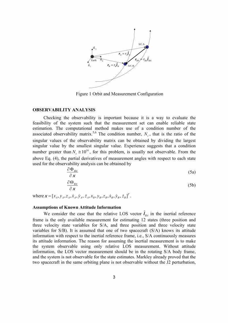
since inclination information is lost for the spherical Earth assumption.4 We considered this attitude knowledge effect, when the J2 perturbation is not included in the dynamical equation. For this case, the orbit configuration of two spacecraft can have an infinite number of possibilities representing the exactly same relative motion measurements, since inclination and the longitude of ascending node are not unique without the J2 effect. However, in the presence of the J2 perturbations, the orbit precession effect is a unique function of inclination, which proves to make the system more observable. In order to check this, a pair of orbit system (two orbit system (a)) is chosen as shown in Table 1. Figure 2 shows the angle measurements in the LVLH frame with respect to variation of ascending node including J2 with both inclinations iA = iB = 45 deg. Even if the J2 perturbation is included for the analysis the measurements are not unique and the system is still unobservable with the measurements in the LVLH frame (the condition number is about 1017). Figure 3 shows that the inertial angle measurements can be separated even without J2 perturbation. Therefore, this two spacecraft system requires knowledge of attitude information of one of two spacecraft. For the inertial measurement when the attitude information of S/A is available, the position and velocity vectors of two spacecraft system is numerically observable without the J2 perturbation even if the two orbits are in the same orbiting plane (as long as inclination is not equal to 0 deg for both spacecraft) and the eccentricity is not 0 for at least one of two spacecraft (for this case, the condition number is about 1012, which means observable). When two orbits are not in the same plane, the system is completely observable without J2 perturbation. Including J2 makes the system more observable and the higher inclination configuration for both spacecraft is more observable than the lower inclination configuration. The system is weakly observable when two orbits are on the same plane and have the same eccentricity.

Table 1 THE TWO ORBIT SYSTEM (a)

a (km) e i (deg) Ω (deg) ω (deg) M0 (deg) Period (sec) S/A 4101.5× 0.1 45 30 20 5.0 4101.8283× S/B 4101.5× 0.1 45 30 10 1.0 4101.8283×

0 0.5 1 1.5 2

x 104

90

95

100

105

110

115

120

125

Time (sec)

LVLH

Azi

mut

h A

ngle

(deg

)

ΩA = 10 deg, ΩB = 40 degΩA = 20 deg, ΩB = 50 degΩA = 30 deg, ΩB = 60 deg

0 0.5 1 1.5 2

x 104

-80

-60

-40

-20

0

20

40

60

80

Time (sec)

LVLH

Ele

vatio

n A

ngle

(deg

)

ΩA = 10 deg, ΩB = 40 degΩA = 20 deg, ΩB = 50 degΩA = 30 deg, ΩB = 60 deg

Figure 2 Angle Measurements with J2 in the LVLH frame

5

0 0.5 1 1.5 2

x 104

-200

-150

-100

-50

0

50

100

150

200

Time (sec)

Iner

tial A

zim

uth

Ang

le (d

eg)

ΩA = 10 deg, ΩB = 40 degΩA = 20 deg, ΩB = 50 degΩA = 30 deg, ΩB = 60 deg

0 0.5 1 1.5 2

x 104

-30

-20

-10

0

10

20

30

Time (sec)

Iner

tial E

leva

tion

Ang

le (d

eg)

ΩA = 10 deg, ΩB = 40 degΩA = 20 deg, ΩB = 50 degΩA = 30 deg, ΩB = 60 deg

Figure 3 Angle Measurements without J2 in the inertial frame

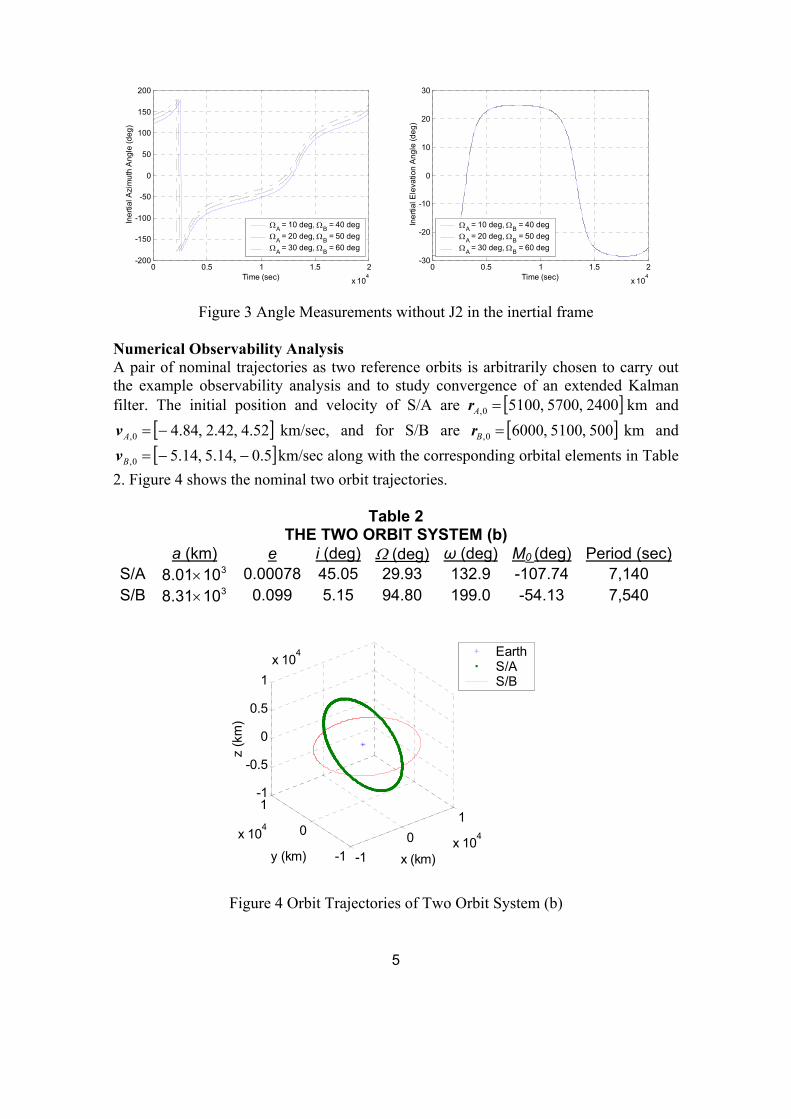
Numerical Observability Analysis A pair of nominal trajectories as two reference orbits is arbitrarily chosen to carry out the example observability analysis and to study convergence of an extended Kalman filter. The initial position and velocity of S/A are [ ]2400,5700,51000, =Ar km and

[ ]52.4,42.2,84.40, −=Av km/sec, and for S/B are [ ]500,5100,60000, =Br km and [ ]5.0,14.5,14.50, −−=Bv km/sec along with the corresponding orbital elements in Table

2. Figure 4 shows the nominal two orbit trajectories.

Table 2 THE TWO ORBIT SYSTEM (b)

a (km) e i (deg) Ω (deg) ω (deg) M0 (deg) Period (sec)S/A 3108.01× 0.00078 45.05 29.93 132.9 -107.74 7,140 S/B 3108.31× 0.099 5.15 94.80 199.0 -54.13 7,540

-10

1

x 104

-1

0

1

x 104

-1

-0.5

0

0.5

1x 104

x (km)y (km)

z (k

m)

EarthS/A S/B

Figure 4 Orbit Trajectories of Two Orbit System (b)

6

The observability of the nominal two orbit system (b) is investigated by obtaining the condition number of singular values. The largest singular value is 63.3 and the smallest singular value is ,1000.7 10−× and therefore, the condition number for the case is 10101.9 × . The state variables corresponding to each singular value can be found from the singular vector matrix V of the singular value decomposition. A state variable corresponding to a larger singular value is more observable than a state variable corresponding to a smaller value. For the two spacecraft system, the well observable states are Az& , Bz& , Ax& , Bx& , and the less observable states are Az , Ay , By . A property of this two orbit system is that the states for the two orbits are coupled to each other such that if Az& , Ax& are the most observable state variables then Bz& , Bx& are also observable with almost same degree. As a whole, it can be concluded that the velocity components of S/A and S/B are the most observable and the position of S/A ( Az , Ay ) is the least observable.

The observablility of the two spacecraft system with respect to varying orbital elements was checked. The measurement is only the relative LOS vector between the spacecrafts. In order to check this orbital element effect on the observability, the two orbit system (a) with comparably larger semimajor axis than the two orbit system (b) is used for considering the physically meaningful orbit configuration for the case of varying eccentricity (with large eccentricity). For gaining knowledge of the effect of semimajor axis on observability, while the semimajor axis of S/A is retained at 15,000 km, only the semimajor axis of S/B is changed from 10,000 km to 20,000 km at 1,000 km intervals and the nominal values of other orbital elements are used. The condition numbers are obtained from the observability matrices. Investigating the condition numbers reveals that when two spacecraft are comparably close, the observability decreases since the two orbits are influenced to about the same degree by the nonspherical Earth assumption such that the system is less observable when the two orbits are in the same orbiting plane. The most observable state variables are the velocity components for both orbits Az& , Bz& , except at semimajor axis equal to 12,000 km ( Bx& , Ax& ) and 13,000 km ( By& , Ay& ). The least observable state variables are apparently the position Ay and By and for some cases Ax and Bx . Since the semimajor axes are not equal; the periods of the two orbits differ. As a consequence, the LOS vector between these spacecrafts will be obstructed by the Earth part of the time. This visibility issue was not considered here but obviously must be in practice.

In order to obtain the effect of eccentricity on observablility, the eccentricity of S/A and S/B varies from 0.1 to 0.6 at intervals 0.1 with the fixed semimajor axis of 15,000 km for both orbits. For obtaining the observability result from the effect of only eccentricity, the inclination for both orbits is set to be 0 deg and eccentricity 0 is avoided for the system to be more observable (i.e., having relatively smaller condition number) and to show the reasonable range of condition numbers. The result reveals that the observability degrades when the two orbits have the same eccentricity, while the observability increases on the whole when the difference of eccentricity between two spacecrafts increases. The most observable state variables are the same, Az& , Bz& as the case for variation of semimajor axis and the least observable are Ax for high eccentricity

7

of S/B and By for high eccentricity of S/A. Again, for the least observable state variables are Ax , By .

For inclination, the inclination of S/A and S/B varies from 10 deg to 80 deg with 10 deg intervals. In order to extract the pure effect of inclination, the eccentricity of orbits is assumed to be zero. It is found that when the nonzero eccentricity is used, the result obtained shows some different trends. The system is weakly observable when the orbits have the same inclination. For the lower inclination (10 deg) of S/A, as the inclination of S/B goes higher, the most observable state variables are changed from Az& or Bz& to Ax& , By& and Ay& . For the medium inclination (20 deg ~ 40 deg) of S/A, the most observable state variable is Bz& for almost inclination cases of S/B with several exceptions. For the case of the higher inclination of S/A and the lower inclination of S/B, the most observable state variable is Bx& . For the high inclination of S/A (80 deg), the most state variable is By& for the inclination 10 deg ~ 30 deg of S/B, and it is Bx& for the higher inclination (> 40 deg) of S/B. When the two orbits are in the same plane, i.e., having same inclinations, the most observable state variable is Az& up to the inclination 50 deg and for the higher inclination, it is changed to Bx& . For the lower inclination of S/A and the higher inclination of S/B, By is the least observable, and for the higher inclination of S/A and the lower inclination of S/B, Bx is the least observable. When the two orbits are in the same plane, Az is the least observable up to 40 deg inclination and for higher inclination, it changes to By .

ERROR COVARIANCE ANAYSIS

Error covariance analysis based on an extended Kalman filter was considered in order to infer the filter performance with solely the initial state error and the measurement error. The covariance propagation from an extended Kalman filter7,8 is introduced in this section and also used in the next section for the Kalman filter simulation studies. The standard orbit model in Eq. (1) can be written in the general state equation form which can be used for the state propagation in the filter as

kk ttttt <<+= −1),(),( wxfx& (6) where x is a state vector and w is a white Gaussian process noise term. In general, the discrete measurement equation can be expressed for the filter as

kkkkk t vxhy += ),(~ (7) where ky~ is a measurement vector and kv is a measurement noise which is assumed to be a white Gaussian noise process. The error covariance matrix can be expressed as

( ) [ ][ ][ ]TttttEtP )()(ˆ)()(ˆ xxxx −−= (8) When the first-order expansion is used for the above nonlinear equations, Eqs. (6) and (7), we have

wxx GF += δδ& (9a) kk H vxy += δδ~ (9b)

8

where the Jacobians are xf∂∂

≡F , wf

∂∂

≡G , xh∂∂

≡H and we assume a zero mean white

noise process and measurement noise with known covariance matrices: QE T =ww (10a) RE T

kk =vv (10b) where w and v are assumed to be uncorrelated with each other and with their previous values over time, and Q and R are the process noise covariance matrix and the measurement noise covariance matrix, respectively. Then the state covariance with initial state error and measurement error propagates with time using the nonhomogeneous Lyapunov differential equation

TT GQGPFFPP ++=& (11) and for a discrete time the covariance is alternatively represented by

TTk GQGPP +ΦΦ=− (12)

The forward propagated state covariance of Eq. (12) is updated when the measurement is available as follows

[ ] −+ −= kkkk PHKIP (13a) [ ]RHPHHPK T

kkkTkkk += −− (13b)

where −kP is an error covariance matrix before the update which comes from the

integration of the Eq. (11) or from the calculation of the Eq. (12) and +kP is an updated

error covariance matrix. For covariance propagation, the state vector is propagated using Eq. (6) and the linearized matrices F and H are evaluated with respect to the true nominal state values since the state estimates are not performed.

The error covariance is propagated with 5% initial state error for each state variable, the relative LOS measurement error standard deviation of 51075.1 −× rad, and the process noise covariance 1212

15101 ×− ⋅×= IQ . The propagation results are shown in

Figures 5 and 6. In order to show obviously the convergence trend, a logarithmic (base 10) scale is used for the y-axis, the square roots of the covariance errors. Table 3 shows the covariance error at final time, and the largest error is for Ay and Bz .

0 2000 4000 6000 8000 10000

10-1

100

101

Time (sec)

S/A

Pos

ition

Erro

r (km

)

xyz

0 2000 4000 6000 8000 10000

10-4

10-3

10-2

Time (sec)

S/A

Vel

ocity

Erro

r (km

/sec

)

xyz

Figure 5 Covariance Propagation of S/A

9

0 2000 4000 6000 8000 10000

10-1

100

101

Time (sec)

S/B

Pos

ition

Erro

r (km

)xyz

0 2000 4000 6000 8000 10000

10-4

10-3

10-2

Time (sec)

S/B

Vel

ocity

Erro

r (km

/sec

)

xyz

Figure 6 Covariance Propagation of S/B

Table 3

COVARIANCE PROPAGATION ERROR S/A Covariance Error S/B Covariance Error

Ax 0.0343 (km) Bx 0.0242 (km)

Ay 0.0444 (km) By 0.0425 (km)

Az 0.0165 (km) Bz 0.0509 (km)

Ax& 5102.24 −× (km/sec) Bx& 5−×104.61 (km/sec) Ay& 5106.04 −× (km/sec) By& 5101.48 −× (km/sec) Az& 5−×106.93 (km/sec) Bz& 5−×106.24 (km/sec)

The effect of measurement frequency on the covariance error propagation has

been checked by using the different measurement sampling time dt = 100, 50, 20, 10, and 5 seconds with the same initial and final time, and obtaining the final time covariance error (Table 4). As expected, using the smaller measurement time step gives a more accurate covariance error. The final time covariance error decreases when the smaller sampling time (and a greater number of measurements) is used. Nonetheless, the accuracy improvement is not so effective as much as the measurement sampling time decreases for the calculation. This is the reason that the sampling time 20 second is chosen for the measurement updates.

Table 4

COVARIANCE PROPAGATION ERROR VS. MEASUREMENT FREQUENCY Sampling Time (sec) Position Error (km) Velocity Error (km/sec)

100 0.189 4102.26 −× 50 0.143 4−×101.86 20 0.0916 4−×101.23 10 0.0674 5−×109.06 5 0.0534 5−×107.06

10

For measurement accuracy, only the relative LOS vectors are considered as available measurements, measured in the inertial reference system. By changing the LOS measurement accuracy from 51075.1 −×=aσ rad (Case 1), 41075.1 −×=aσ rad (Case 2), and 31075.1 −×=aσ rad (Case 3), the final time covariance error for each state is obtained as shown in Table 5. As the accuracy of the relative LOS vector is degraded by one order of magnitude, the final time covariance error increases about one order. It means that the accuracy of the state estimation directly depends on the accuracy of measurement sensor, as expected. Therefore, the development of accurate LOS sensors is very essential to this system estimates.

Table 5

COVARIANCE PROPAGATION ERROR VS. MEASUREMENT ACCURACY Cases Position Error (km) Velocity Error (km/sec) Case 1 0.0916 4101.23 −× Case 2 0.902 3101.22 −× Case 3 9.02 2101.22 −×

EXTENDED KALMAN FILTER

The extended Kalman filter simulation is performed for the two spacecraft system. Since in the previous section, some part of an extended Kalman filter has already been introduced, we introduce only the state update part. In the extended Kalman filter, the state can be updated when new measurements are available using the equation8:

( )[ ]−−+ −+= kkkkkk K xhyxx ˆ~ˆˆ (14) where the superscripts + and - denote the estimates after the measurement update and the propagated estimates at the update time, respectively, and kK is a gain at the measurement time update given by

[ ]RHPHHPK Tkkk

Tkkk += −− (15)

and here +kP is an updated error covariance matrix

[ ] −+ −= kkkk PHKIP 16) and −

kP is an error covariance matrix before the update which comes from the integration of the following equation

.TT GQGPFFPP ++=& (17) Also, the state propagation is given by the following equation

( ).,ˆ tx xf=& (18) Equations (14)-(18) represent the extended Kalman filter that is used to estimate the orbital position and velocity. We note that the nonlinear system in Eq. (18) is integrated forward as the updated nominal trajectory estimate from +

−1ˆ kx to −kx obtain to use in the

update of Eq. (14). The various jacobians and state transition matrices (used in the covariance updates and Kalman gain) are all evaluated using the most recent nominal state trajectory estimates.

11

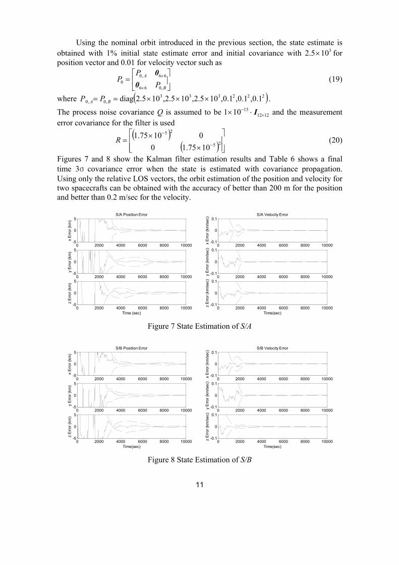
Using the nominal orbit introduced in the previous section, the state estimate is obtained with 1% initial state estimate error and initial covariance with 3105.2 × for position vector and 0.01 for velocity vector such as

=

×

×

B

A

PP

P,066

66,00 0

0 (19)

where ( )222333,0,0 1.0,1.0,1.0,102.5,102.5,102.5diag ×××== BA PP .

The process noise covariance Q is assumed to be 121215101 ×

− ⋅× I and the measurement error covariance for the filter is used

( )( )

××=

−

−

25

25

1075.1001075.1R (20)

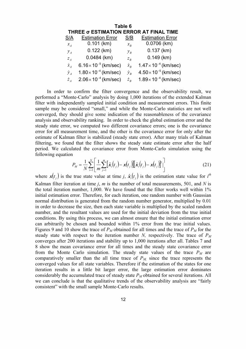
Figures 7 and 8 show the Kalman filter estimation results and Table 6 shows a final time 3σ covariance error when the state is estimated with covariance propagation. Using only the relative LOS vectors, the orbit estimation of the position and velocity for two spacecrafts can be obtained with the accuracy of better than 200 m for the position and better than 0.2 m/sec for the velocity.

0 2000 4000 6000 8000 10000-5

0

5S/A Position Error

x E

rror (

km)

0 2000 4000 6000 8000 10000-5

0

5

y E

rror (

km)

0 2000 4000 6000 8000 10000-5

0

5

Time (sec)

z E

rror (

km)

0 2000 4000 6000 8000 10000-0.1

0

0.1S/A Velocity Error

x E

rror (

km/s

ec)

0 2000 4000 6000 8000 10000-0.1

0

0.1

y E

rror (

km/s

ec)

0 2000 4000 6000 8000 10000-0.1

0

0.1

Time(sec)

z E

rror (

km/s

ec)

Figure 7 State Estimation of S/A

0 2000 4000 6000 8000 10000-5

0

5S/B Position Error

x E

rror (

km)

0 2000 4000 6000 8000 10000-5

0

5

y E

rror (

km)

0 2000 4000 6000 8000 10000-5

0

5

Time(sec)

z E

rror (

km)

0 2000 4000 6000 8000 10000-0.1

0

0.1S/B Velocity Error

x E

rror (

km/s

ec)

0 2000 4000 6000 8000 10000-0.1

0

0.1

y E

rror (

km/s

ec)

0 2000 4000 6000 8000 10000-0.1

0

0.1

Time(sec)

z E

rror (

km/s

ec)

Figure 8 State Estimation of S/B

12

Table 6 THREE σ ESTIMATION ERROR AT FINAL TIME

S/A Estimation Error S/B Estimation Error Ax 0.101 (km) Bx 0.0706 (km)

Ay 0.122 (km) By 0.137 (km)

Az 0.0484 (km) Bz 0.149 (km)

Ax& 5106.16 −× (km/sec) Bx& 4101.47 −× (km/sec) Ay& 4101.80 −× (km/sec) By& 5104.50 −× (km/sec) Az& 4102.06 −× (km/sec) Bz& 4101.89 −× (km/sec)

In order to confirm the filter convergence and the observability result, we

performed a “Monte-Carlo” analysis by doing 1,000 iterations of the extended Kalman filter with independently sampled initial condition and measurement errors. This finite sample may be considered “small,” and while the Monte-Carlo statistics are not well converged, they should give some indication of the reasonableness of the covariance analysis and observability ranking. In order to check the global estimation error and the steady state error, we computed two different covariance errors; one is the covariance error for all measurement time, and the other is the covariance error for only after the estimate of Kalman filter is stabilized (steady state error). After many trials of Kalman filtering, we found that the filter shows the steady state estimate error after the half period. We calculated the covariance error from Monte-Carlo simulation using the following equation

( ) ( )[ ] ( ) ( )[ ]∑ ∑= =

−−=

N

i

Tjji

m

jjjiM tttt

mNP

1 1

ˆˆ11 xxxx (21)

where ( )jtx is the true state value at time j, ( )ji tx is the estimation state value for ith Kalman filter iteration at time j, m is the number of total measurements, 501, and N is the total iteration number, 1,000. We have found that the filter works well within 1% initial estimation error. Therefore, for each iteration, one random number with Gaussian normal distribution is generated from the random number generator, multiplied by 0.01 in order to decrease the size, then each state variable is multiplied by the scaled random number, and the resultant values are used for the initial deviation from the true initial conditions. By using this process, we can almost ensure that the initial estimation error can arbitrarily be chosen and bounded within 1% error from the true initial values. Figures 9 and 10 show the trace of PM obtained for all times and the trace of PM for the steady state with respect to the iteration number N, respectively. The trace of PM converges after 200 iterations and stability up to 1,000 iterations after all. Tables 7 and 8 show the mean covariance error for all times and the steady state covariance error from the Monte Carlo simulation. The steady state values of the trace PM are comparatively smaller than the all time trace of PM, since the trace represents the converged values for all state variables. Therefore if the estimation of the states for one iteration results in a little bit larger error, the large estimation error dominates considerably the accumulated trace of steady state PM obtained for several iterations. All we can conclude is that the qualitative trends of the observability analysis are “fairly consistent” with the small sample Monte-Carlo results.

13

Table 7 MEAN COVARIANCE ERROR

S/A Covariance Error S/B Covariance Error Ax 7.52 (km) Bx 8.54 (km)

Ay 11.5 (km) By 11.8 (km)

Az 7.59 (km) Bz 1.76 (km)

Ax& 0.0107 (km/sec) Bx& 0.0111 (km/sec)

Ay& 0.0103 (km/sec) By& 0.0143 (km/sec)

Az& 0.0100 (km/sec) Bz& 3102.16 −× (km/sec)

Table 8 STEADY STATE COVARIANCE ERROR

S/A Covariance Error S/B Covariance Error Ax 0.0913 (km) Bx 0.137 (km)

Ay 0.343 (km) By 0.121 (km)

Az 0.173 (km) Bz 0.331 (km)

Ax& 4−×101.12 (km/sec) Bx& 4101.05 −× (km/sec) Ay& 4101.82 −× (km/sec) By& 4−×101.11 (km/sec) Az& 4102.15 −× (km/sec) Bz& 4101.72 −× (km/sec)

0 200 400 600 800 10000

200

400

600

800

1000

Iteration Number N

Trac

e P

M

0 200 400 600 800 10000

0.1

0.2

0.3

0.4

0.5

Iteration Number N

Trac

e P

M o

f Ste

ady

Sta

te

Figure 9 Trace of PM Figure 10 Trace of PM for the Steady State

CONCLUSION

Autonomous spacecraft orbit navigation was considered for two spacecraft system using the relative LOS vector between two spacecrafts. Observability of the system was checked in the sense of numerical method. In the computational study, this system requires knowledge of attitude information of one of two spacecrafts. For the inertial measurement when the attitude information of S/A is available, the two spacecraft system can be observable without J2 perturbation as long as two orbits are not in the same orbiting plane i = 0 deg. Including J2 makes the system more observable and the

14

higher inclination configuration for both spacecraft is more observable than the lower inclination configuration. The system is weakly observable when two orbits are on the same plane and have the same eccentricity. Error covariance analysis based on an extended Kalman filter was considered and the estimation accuracy directly depends almost linearly on the accuracy of the relative LOS vector measurement. For the nominal two spacecraft system, the extended Kalman filter simulations were performed and the filter estimation was obtained with an accuracy of about 200 m for the position and about 0.2 m/sec for the velocity. This estimation results were confirmed by the Monte-Carlo simulation. The concept of two spacecraft orbit estimation can be extended to orbit estimation for formation flying spacecraft system, and the relative position estimation in the spacecraft body frame can be considered as further research. Throughout this research, the results clearly show that a fully autonomous on-board orbit navigation system is feasible by using an electro-optical means for measuring the relative LOS vector.

REFERENCES

1. Chory, M. A., Hoffman, D. P., Major, C. S., and Spector, V. A., “Autonomous Navigation – Where We Are in 1984,” AIAA Guidance and Control Conference, AIAA Seattle, WA, Aug. 1984, pp. 27-37, AIAA Paper 84-1826.

2. Markley, F. L., ‘‘Autonomous Satellite Navigation Using Landmark,’’ AAS/AIAA Astrodynamics Conference, North LakeTahoe, NV, Aug. 1981. pp.989-1010, AAS Paper 81-205

3. Markley, F. L., ‘‘Autonomous Navigation Using Landmark and Intersatellite Data,’’ AIAA/AAS Astrodynamics Conference, Seattle, WA, Aug. 1984, pp. 111, AIAA Paper 84-1987.

4. Psiaki, M. L., ‘‘Autonomous Orbit Determination for Two Spacecraft from Relative Position Measurements,’’ Journal of Guidance, Control, and Dynamics, Vol. 22, No. 2, 1999, pp. 305-312.

5. Yim, J. R., ‘‘Autonomous Spacecraft Orbit Navigation,’’ Ph. D. Dissertation, Texas A&M University, 2002.

6. Yim, J. R., Crassidis, J. L., and Junkins, J. L., “Autonomous Orbit Navigation of Interplanetary Spacecraft,” AIAA/AAS Astrodynamics Specialist Conference, Denver, CO, Aug. 2000, pp. 53-61, AIAA Paper 2000-3936.

7. Gelb, A., Applied Optimal Estimation, The M.I.T. Press, Cambridge, MA, 1974, pp. 182-190.

8. Junkins, J. L., an Introduction to Optimal Estimation of Dynamical Systems, Sijthoff & Noordhoff International Publishers B.V., Alphen aan den Rijn, The Netherlands, 1978, pp. 200-203.