Aalborg Universitet

Wind turbine state estimation

Knudsen, Torben

Publication date:2014

Document VersionEarly version, also known as pre-print

Link to publication from Aalborg University

Citation for published version (APA):Knudsen, T. (2014). Wind turbine state estimation.

General rightsCopyright and moral rights for the publications made accessible in the public portal are retained by the authors and/or other copyright ownersand it is a condition of accessing publications that users recognise and abide by the legal requirements associated with these rights.

- Users may download and print one copy of any publication from the public portal for the purpose of private study or research. - You may not further distribute the material or use it for any profit-making activity or commercial gain - You may freely distribute the URL identifying the publication in the public portal -

Take down policyIf you believe that this document breaches copyright please contact us at vbn@aub.aau.dk providing details, and we will remove access tothe work immediately and investigate your claim.

Downloaded from vbn.aau.dk on: February 21, 2022

Wind Turbine State Estimation

Torben KnudsenAutomation and Control

Department of Electronic SystemsAalborg University

March 26, 2014

Abstract

Dynamic inflow is an effect which is normally not included in the models used for wind turbine controldesign. Therefore, potential improvement from including this effect exists. The objective in this projectis to improve the methods previously developed for this and especially to verify the results using full-scale wind turbine data.

The previously developed methods were based on extended Kalman filtering. This method has severaldrawback compared to unscented Kalman filtering which has therefore been developed. The unscentedKalman filter was first tested on linear and non-linear test cases which was successful. Then the esti-mation of a wind turbine state including dynamic inflow was tested on a simulated NREL 5MW turbinewas performed. This worked perfectly with wind speeds from low to nominal wind speed as the out-put prediction errors where white. In high wind where the pitch actuator was always active the resultswhere not as convincing because the output prediction errors where not white. Using real data it has notbeen possible to get really good results so far. There remains a number of challenges: verifying turbineparameters and getting the most suitable measurement signals, including the 3P effect in the model andperhaps including the 1P effect. It is obviously difficult to make a final conclusion before the abovechallenges has been resolved.

Acknowledgement

This work has been funded by Norwegian Centre for Offshore Wind Energy (NORCOWE) under grant193821/S60 from Research Council of Norway (RCN). NORCOWE is a consortium with partners fromindustry and science, hosted by Christian Michelsen Research. All the data necessary for the full scaleexperiments was kindly provided by Vestas Wind Systems A/S.

1

Contents

1 Introduction 4

1.1 Objectives . . . . . . . . . . . . . . . . . . . . . . . . . . . . . . . . . . . . . . . . . . 4

1.2 Approach and outline . . . . . . . . . . . . . . . . . . . . . . . . . . . . . . . . . . . . 4

2 Continuous discrete unscented Kalman filter 6

2.1 The continuous–discrete KF . . . . . . . . . . . . . . . . . . . . . . . . . . . . . . . . 6

2.2 The continuous–discrete EKF . . . . . . . . . . . . . . . . . . . . . . . . . . . . . . . . 7

2.3 Unscented transform . . . . . . . . . . . . . . . . . . . . . . . . . . . . . . . . . . . . 7

2.4 Unscented Kalman filter . . . . . . . . . . . . . . . . . . . . . . . . . . . . . . . . . . 11

2.5 Test of the UKF implementation . . . . . . . . . . . . . . . . . . . . . . . . . . . . . . 12

3 Dynamic inflow model 16

4 Test based on NREL 5MW simulations 17

4.1 Close to rated wind . . . . . . . . . . . . . . . . . . . . . . . . . . . . . . . . . . . . . 17

4.2 High wind . . . . . . . . . . . . . . . . . . . . . . . . . . . . . . . . . . . . . . . . . . 17

4.3 Summary of results . . . . . . . . . . . . . . . . . . . . . . . . . . . . . . . . . . . . . 17

5 Test based on full-scale data 23

5.1 First data . . . . . . . . . . . . . . . . . . . . . . . . . . . . . . . . . . . . . . . . . . 23

5.2 Second data sets . . . . . . . . . . . . . . . . . . . . . . . . . . . . . . . . . . . . . . . 23

5.3 Low wind . . . . . . . . . . . . . . . . . . . . . . . . . . . . . . . . . . . . . . . . . . 24

5.4 Close to rated wind . . . . . . . . . . . . . . . . . . . . . . . . . . . . . . . . . . . . . 26

5.5 Discussion . . . . . . . . . . . . . . . . . . . . . . . . . . . . . . . . . . . . . . . . . . 30

6 Conclusion 32

2

A Measurement specifications 34

B Parameter specifications 36

C Second order statistics for y = xTx for x Gaussian 37

D Detailed dynamic model 40

3

Chapter 1

Introduction

This report is part of the work done in the NORCOWE project by section for Automation and Control,Department for Electronic Systems, AAU. In the work plan for 2013 the following deliverable “Paperon methods for estimating the effective wind speed and available power at a single turbine.” is listed andcovered by Knudsen and Bak [2013]. The results in this paper suggested new research especially usingunscented instead of extended Kalman filtering and using a standard large commercial wind turbineinstead of a small prototype for experimantal verification. The results of this research is presented in thisreport.

1.1 Objectives

The significance of dynamic inflow is discussed in Knudsen and Bak [2013]. Especially for modelbased control design dynamic inflow could have an important role. The main objective in this projectis to improve and verify the dynamic inflow model presented in Knudsen and Bak [2013]. Initially asecond stage for 2014 was also discussed. This stage would include pursuing possible improvementsfor the inflow model. Moreover, data driven modelling of larger parts of the wind turbine model will beconsidered e.g. improving the Cp and Ct models. This report only covers the first stage.

1.2 Approach and outline

The original state estimator in Knudsen and Bak [2013] is based on a extended Kalman filter (EKF).EKF make use of a linearised state model. This makes it difficult to change the model as new partialderivatives have to be derived. The unscented Kalman filter (UKF) [Julier et al., 1995] uses the un-scented transform [Thrun et al., 2006] to calculate necessary means and covariances and does not needlinearization. Moreover, the UKF should have the same or better performance compared to the EKFdepending on the type of non linearities. For these good reasons the EKF was exchanged with a UKF.In order to keep the parametrisation from the stochastic differential equations (SDE) from physics theEKF was of the continuous-discrete (CD) type i.e. based on the continuous SDE for the state and thediscrete time measurement equation. Exciting implementations of the UKF have only been found for thediscrete-discrete (DD) case i.e. with discrete time state equation. Therefore a CD version of the UKFhas been developed in section 2.4.

4

In Knudsen and Bak [2013] the drive train model is simply a one inertia model. As the drive train is onlyweekly damped drive train oscillations can occur depending on the controller. Therefore the drive trainmodel used here consists of two masses one for the slow rotor part and one for the fast generator part,the two inertias are connected with a spring and damper. This extension and the rest of the model fromKnudsen and Bak [2013] are briefly presented in section 3.

The developed UKF is tested on a “standard” non-linear system in section 2.4. One possible next stepwould be to directly test with full-scale data. An intermediate step taken here is to test the wind turbinestate estimation on simulated data. This makes it possible to check for errors in the wind turbine specificpart of the UKF implementation. When there are no more errors the results shows the performance forthe simulated case which is assumed to be the the upper limit of what can be achieved with real data.The simulation test is presented in section 4.

Finally the UKF is tested on real full-scale data in section 5.

5

Chapter 2

Continuous discrete unscentedKalman filter

This section serves to document the ideas and understanding gained regarding UKF. This can appearrather technical and can be skipped for those who focus more on results.

For reference the basic KF filter for linear systems are first presented below.

2.1 The continuous–discrete KF

Assume the linear time varying system:

dx(t) = (F (t)x(t) +B(t)u(t)) dt+ dw(t) (2.1a)y(tk) = H(tk)x(tk) +D(tk)u(tk) + v(tk) (2.1b)

w(t) ∈W (Q(t)) , v(ti) ∈ N(0, R(ti)) , E(v(ti)v(tj)T) = ∆(ti − tj)R(ti) (2.1c)

and the normal definitions

x(t−k ) , E(x(tk)|Y t−10 ) , (2.2a)

x(t+k ) , E(x(tk)|Y t0 ) , (2.2b)

Y t0 , y(t), y(t− 1), . . . , y(0) (2.2c)

P (t−k ) , Cov(x(tk)|Y t−10 ) = E((x(tk)− x(t−k ))(x(tk)− x(t−k ))T

)(2.2d)

P (t+k ) , Cov(x(tk)|Y t0 ) = E((x(tk)− x(t+k ))(x(tk)− x(t+k ))T

)(2.2e)

Given measurements and initial values:

y(t0), y(t1), y(t2) . . . , y(t), t ≥ t0, (2.3a)

x(t−0 ) = x0 , P (t−0 ) = P0 (2.3b)

The KF can be formulated as follows:

Measurement update at time tk:

K(tk) = P (t−k )H(tk)T(H(tk)P (t−k )H(tk)T +R(tk))−1 (2.4a)

6

x(t+k ) = x(t−k ) +K(tk)(y(tk)−H(tk)x(t−k )−D(tk)u(tk)) (2.4b)

P (t+k ) = (I −K(tk)H(tk))P (t−k )(I −K(tk)H(tk))T +K(tk)R(tk)K(tk)T (2.4c)

Time update from tk to tk+1:

x(tk) = x(t+k ) , P (tk) = P (t+k ) (initial conditions) (2.5a)˙x(t) = F (t)x(t) +B(t)u(t) (diff. eq. for x) (2.5b)

P (t) = F (t)P (t) + P (t)F (t)T +Q(t) (diff. eq. for P ) (2.5c)

x(t−k+1) = x(tk+1) , P (t−k+1) = P (tk+1) (Result) (2.5d)

2.2 The continuous–discrete EKF

Assume now the nonlinear model (2.6).

dx(t) = f(x(t), u(t))dt+ dw(t) (2.6a)y(tk) = h(x(tk), u(tk)) + v(tk) (2.6b)

The extended EKF is then derived from the KF by using the following heuristic principle: use thenonlinear relations when possible and the linearization otherwise.

This means that the following are changed to use the nonlinear equations.

Measurement update at time tk:

x(t+k ) = x(t−k ) +K(tk)(y(tk)− h(x(t−k ), u(tk), tk)) (2.7)

Time update from tk to tk+1:

˙x(t) = f(x(t), u(t), t) (diff. eq. for x) (2.8)

In all the other equations the linearized parameters (2.9) must be used.

F (x, u, t) ,∂f(x, u, t)

∂x(2.9a)

H(x, u, t) ,∂h(x, u, t)

∂x(2.9b)

It is best to use the most recent values of the state estimate, i.e.,

H(tk) = H(tk, x(t−k ), u(t−k )) (2.10)F (t) = F (t, x(t|tk), u(t)) (2.11)

2.3 Unscented transform

The basic new idea in the UKF is to use the unscented transform (UT) to calculate necessary conditionalmeans and covariances in the measurement (2.4) and time update (2.5). The problem solved by the UT is

7

the basic probabilistic problem of calculating the statistics of x, y given the statistics of x and a relationf :

y = f(x) , µx = E(x) , Cx = Cov(x) (2.12)

For non-liner relations there is no exact solution to find even the second order statistics. The EKF can beinterpreted as using the linearization approach:

y ∼ f(µx) +∇f(µx)(x− f(µx))⇒ (2.13)

µy = f(µx) , Cyx = ∇f(µx)Cx , Cy = ∇f(µx)Cx∇f(µx)T (2.14)

A Monte Carlo approach would be to generate random realisations xi based on the statistics for x andestimating the statistics for x, y as follows:

µy =1

N

N∑i=1

f(xi) , µx =1

N

N∑i=1

xi , (2.15)

Cyx =1

N

N∑i=1

(f(xi)− µy))(xi − µx))T , Cy =1

N

N∑i=1

(f(xi)− µy))(f(xi)− µy))T , (2.16)

The UT can be seen as the Monte Carlo method but where the xi’s are not randomly drawn but con-structed to obtain certain features these constructed xi’s are called sigma points. Especially if x isGaussian it is natural to use the eigen vectors of Cx to construct the sigma points. The UT used here isgiven below where n is the dimension of x.

α = 1 , κ = 2 , β = 0 , (Default parameters gives λ= 2) (2.17a)

λ = α2(n+ κ)− n , (2.17b)

k =√n+ λ , (2.17c)

ui , eigenvector i for Cx , li , eigenvalue i for Cx , (2.17d)

xi =

µx , i = 0

µx + kui√li , 1 ≤ i ≤ n

µx − kui√li , n+ 1 ≤ i ≤ 2n

(2.17e)

wti =

λ

n+λ , i = 0 , t = m (for mean)λ

n+λ + 1− α2 + β , i = 0 , t = c (for covarians)1

2(n+λ) , 1 ≤ i ≤ 2n

(2.17f)

µy =

2n∑i=0

wmi f(xi) , (2.17g)

Cyx =

2n∑i=0

wci (f(xi)− µy))(xi − µx))T , (2.17h)

Cy =

2n∑i=0

wci (f(xi)− µy))(f(xi)− µy))T , (2.17i)

Notice that∑2ni=0 w

mi = 1 and for the chosen parameters wmi = wci . This construction can be shown to

give exactly correct results for linear and affine functions f(x) = Ax+ b. Here eigen vectors are used to

8

construct the sigma points. There are other ways, e.g. Cholesky factorisation, which gives correct resultsfor linear functions but different results for non-linear functions.

The above UT has been tested and compared to both the MC method and the version using Choleskyfactorisation. A number of different functions f(x) has been tested. In general the two versions of theUT transform are quit similar. In order to have a test where the correct result is known the E(y) andCov(y, x) is derived in appendix C for y = xTx. The results are shown in figure 2.1– 2.3 and table 2.1for the Gaussian case with E(x) = [1; 1] and Cov(x) = [1 1; 1 2] (using Matlab notation).

−8 −6 −4 −2 0 2 4 6 8 10

−2

0

2

4

Sigma points x

−30 −20 −10 0 10 20 30

5

10

15

20

Mapped sigma points y

Figure 2.1: Sigma points and images for the UT based on (2.17).

Method My Cy CyxUTSCEst 5.000e+00 3.900e+01 4.000e+00 6.000e+00UTJMEst 5.000e+00 3.100e+01 4.000e+00 6.000e+00

UTMCEst 5.038e+00 3.385e+01 3.988e+00 6.028e+00THTK 5.000e+00 3.400e+01 4.000e+00 6.000e+00

UTSCRelE 0 1.471e-01 0 0UTJMRelE 0 -8.824e-02 0 0

UTMCRelE 7.663e-03 -4.284e-03 -3.090e-03 4.670e-03

Table 2.1: Performance for the above method, the Cholesky based, the MC and the theoretical. The rowsmarked RelE are the errors relative to the correct results.

9

−20 −15 −10 −5 0 5 10 15 20

−5

0

5

MC points x

−100 −50 0 50 100

0

20

40

60

Mapped MC points y

Figure 2.2: Sigma points and images for the MC based method.

−4 −2 0 2 4 6

−4

−3

−2

−1

0

1

2

3

4

5

6

Sigma points

Eigen valuesCholesky

Figure 2.3: Comparision of sigma points based on eigenvalues and the Cholesky method.

10

2.4 Unscented Kalman filter

To understand the UKF it is necessary to follow the derivation of the KF to recognise that the measure-ment update (2.4b) and (2.4c) originates from basic relation for Gaussian variables. Assume x, y areGaussian vectors then the least mean square (LMS) error estimate for x given y is the conditional meanE(x|y).

E(x|y) = E(x) + Cov(x, y) Cov(y)−1(y − E(y)) , (2.18a)

Cov(x|y) = Cov(x)− Cov(x, y) Cov(y)−1 Cov(y, x) , (2.18b)

where

Cov(x, y) , E((x− E(x))(y − E(y))T

), (2.18c)

Cov(x) , Cov(x, x) (2.18d)

If some information z is already available and some new information y will be obtained the similarformulas are

E(x|y, z) = E(x|z) + Cov(x, y|z) Cov(y|z)−1(y − E(y|z)) , (2.19a)

Cov(x|y, z) = Cov(x|z)− Cov(x, y|z) Cov(y|z)−1 Cov(y, x|z) (2.19b)

Applying this where x, y, z are x(tk), y(t−k ), Y t−10 gives the following

x(t+k ) = x(t−k ) + Cov(x(t−k ), y(t−k )) Cov(y(t−k ))−1y(t−k ) , (2.20a)

P (t+k ) = P (t−k )− Cov(x(t−k ), y(t−k )) Cov(y(t−k ))−1 Cov(y(t−k ), x(t−k )) , (2.20b)

y(t−k ) , y(tk)− E(y(tk)|Y t−10 ) = y(tk)−H(tk)x(t−k )−D(tk)u(tk)) , (2.20c)

x(t−k ) , x(tk)− E(x(tk)|Y t−10 ) , (2.20d)

Cov(x(tk), y(t−k )|Y t−10 ) = Cov(x(t−k ), y(t−k )) , (2.20e)

Cov(y(t−k )|Y t−10 ) = Cov(y(t−k )) (2.20f)

this can be verified in the linear case using:

K(tk) = Cov(x(t−k ), y(t−k )) Cov(y(t−k ))−1 , (2.21a)

Cov(y(t−k )) = H(tk)P (t−k )H(tk)T +R(tk) (2.21b)

The UKF measurement update, corresponding to (2.4b)–(2.4c) in the linear case, are given by (2.20a)–(2.20b) where the UT for the measurement equation

y(tk) = h(x, u) + v = ha([x, v], u) (2.22)

with the input statistics

E

(xv

)=

(x(t−k )

0

), (2.23)

Cov

(xv

)=

(P (t−k ) 0

0 R(tk)

)(2.24)

11

gives the output-input statistics

y(t−k ) , Cov(y(t−k ), x(t−k )) = Cov(x(t−k ), y(t−k ))T , Cov(y(t−k )) (2.25)

which are necessary in the UKF measurement update (2.20a)–(2.20b).

The UKF time update using UT calls for a function definition of this step. From a mathematical pointof view the input to this function is x(t−k ), P (t−k ), u(t), t ∈ [tk, tk+1], Q(t), t ∈ [tk, tk+1]. The firsttwo inputs comes from the measurement update step just explained and the two last inputs are assumedknown. The output of the function must be the result of integrating the state SDE (2.26) from tk to tk+1.

dx(t) = f(x(t), u(t))dt+ dw(t) (2.26)

As w is a Wiener process it has independent increments with variance V(w(t + δt) − w(t)) = Q(t)δt.This can be approximated using Runge-Kutta (RK4) integration of the difference equation

δx(t) = f(x(t), u(t))δt+ δw(t) (2.27)δx(t) = (f(x(t), u(t)) + δw(t)/δt)δt (2.28)δx(t) = (f(x(t), u(t)) + δw(t)/δt)δt (2.29)δx(t) = (f(x(t), u(t)) + n(t))δt (2.30)

n(t) should then be a process with independent increments and variance Q(t)(δt)−1. If the (RK4)integration has ni intermediate steps the final state

xf (tk+1) = fa([xi(tk),Ntk+1

tk], U

tk+1

tk) (2.31)

will be a function of the initial state and stacked noise N and input U for the intermediate time steps inthe integration and the UT transform can be used with the input statistics

E

(xiN

)=

x(t−k )

0...0

, (2.32)

Cov

(xiN

)=

P (t−k ) 0 . . . 0

0 Q(tk)/δt . . . 0

0 . . .. . . 0

0 . . . . . . Q(tk+1)/δt

(2.33)

gives the output-input statistics

x(t−k+1) , P (t−k+1) = Cov(x(t−k+1) (2.34)

which are necessary in the UKF time update corresponding to (2.5).

As seen above the UKF can be interpreted as using the UT to calculate the conditional means, variancesand covariances necessary in the KF.

2.5 Test of the UKF implementation

The UKF described above has been turned into a MATLAB program. A DD version has also been madeand then, from previous development, we have both EKF and KF also in both a DD and CD version.

12

To test the CD UKF developed above a number of simulations of SDE has been done. Simulation withlinear SDE’s shows that all KF versions behaves as expected and produces white residuals. This justserves to rule out programming errors. Two non-linear SDE has also been tested. One with polynomialnon-linearities and a Lorenz system with noise. In all cases the CD UKF performed at least as well asthe other KF measured by state prediction error RMS and output prediction error whiteness. In manycases CD UKF was very superior. There were also cases where the CD UKF was much better than theDD UKF even though only one step in the RK4 integration was used.

Below some results from the Lorenz SDE (2.35) are shown.

dx = f(x)dt+ dw , (2.35a)y = x+ v , (2.35b)

f(x) =

σ(x2 − x1)x1(ρ− x3)− x2x1x2 − βx3

, (2.35c)

w ∈W(0, Q) , (2.35d)v ∈ NID(0, R) , (2.35e)

σ = 10 , ρ = 8 , β = 8/3 , Q = 0.12I , R = I , Ts = 0.01 , x(0) =(−1 3 4

)T(2.35f)

As seen in figure 2.4– 2.7 the results are good as everything is as expected e.g. white noise test is OK

−20

−10

0

10

20

−40

−20

0

20

40

0

10

20

30

40

50

Lorenz system

States

Measurements

Figure 2.4: Simulated states and measurements for the Lorenz system.

and also the rms on state prediction errors is close to the average covariances calculated by the UKF. Forthe three states the fraction between rms and calculated covariances are 0.95, 0.94, 1.06 respectively.

13

0 20 40−1

0

1

lag

nobs= 900, p= 0.068246

−50 0 50−0.1

0

0.1

lag

nobs= 900

−50 0 50−0.1

0

0.1

lag

nobs= 900

0 20 40−1

0

1

lag

nobs= 900, p= 0.94597

−50 0 50−0.1

0

0.1

lag

nobs= 900

0 20 40−1

0

1

lag

nobs= 900, p= 0.4622

Figure 2.5: Whiteness test for residuals.

0 200 400 600 800 1000−5

0

5

0 200 400 600 800 1000−5

0

5

Residuals with 2 standard deviations error bounds

0 200 400 600 800 1000−5

0

5

Figure 2.6: Output prediction errors (residuals) vs time including 0.95 confidence limits.

14

0 200 400 600 800 1000−0.5

0

0.5

0 200 400 600 800 1000−1

0

1

State prediction errors with 2 standard deviations error bounds

0 200 400 600 800 1000−1

0

1

Figure 2.7: State prediction errors (residuals) vs time including 0.95 confidence limits.

15

Chapter 3

Dynamic inflow model

To use the UKF for estimating wind turbine states, a state and measurement equation corresponding to(2.6), is needed. The model is a extension of the one used in Knudsen and Bak [2013]. it is explained ingeneral terms in this section. The mathematical details can be found in Knudsen and Bak [2013] and inappendix D where the extension is included.

The dynamic part of the model can be split into disturbance i.e. wind flow, input actuators, control subjecti.e. mechanics and output part. The ambient wind speed is modelled as a mean part which is integratedwhite noise plus the turbulence which has a Kaimal spectrum. The dynamic inflow is modelled via ainduction factor which is a first order filtering of the static induction factor. The input are measured pitchand generator torque and not their reference values so there is no reason to include input dynamics alsothe noise on the inputs are assumed negligible. The mechanics is modelled with a 2 DOF drive trainand a 1 DOF tower fore-aft model. In the original model in Knudsen and Bak [2013] only one DOF(inertia) was used for the drive train. The outputs consists of generator speed, nacelle wind speed andnacelle fore AFT acceleration all with noise but no dynamics. Notice that 1P and 3P disturbances in themeasurements are not considered. For simulation all the parameters are obtained from the model. Forfull-scale most of the parameters are obtained from the manufacturer while the rest, e.g. for the noisepart, are guessed and estimated.

16

Chapter 4

Test based on NREL 5MW simulations

In advance it is not known how well the UKF performs or if it works at all. The theoretical optimalknown performance for KF estimators only applies to linear systems. For non-linear systems we canonly hope for good performance. For this reason the UKF will be tested using simulated data to see theperformance under ideal conditions.

For this a Simulink implementation of the model in section 3 has been used. Notice that the modeland system is then the same. The challenge for the UKF is then the non-linearities not any unmodeleddynamics.

There are some differences in performance depending on the mean wind speed. Therefore examples ofrated (medium) and high wind speed are shown below.

4.1 Close to rated wind

At mean wind speed 11 m/s the pitch is not always active as seen in figure 4.1. For this situation theUKF performs as for a linear system so state predictions stays within calculated confidence intervals asshow for the induction in figure 4.3 and all residuals are white as seen in figure 4.4.

4.2 High wind

In high winds where the pitch is mostly active the performance is not that close to ideal as seen for meanwind speed 15 m/s in figure 4.5–4.8.

4.3 Summary of results

The results in section 4.1– 4.2 are examples of the general picture shown in table 4.1. Here it is clearlyseen that the performance of the UKF depart more from the ideal as the pitch activity, and the meanwind, increases.

There is to possible causes for this disappointing performance:

17

0 1000 2000 3000 4000 5000 60000

1

2

3

4

5

6

7

Input

Pitch(deg)PGen(MW)

Figure 4.1: Input for the NREL 5MW simulated test at mean wind 11m/s.

0 1000 2000 3000 4000 5000 6000−5

0

5

10

15

20

25

Measurements

Omegag(rad/s)x0.1Vn(m/s)An(m/s2)

Figure 4.2: Measurements for the NREL 5MW simulated test at mean wind 11m/s.

18

0 1000 2000 3000 4000 5000 6000−0.05

0

0.05

0.1

0.15

0.2

0.25

0.3

0.35

0.4

0.45

X XHM for the induction factor

aa

a− 2σaa+ 2σa

Figure 4.3: Induction factor and confidense limits for the NREL 5MW simulated test at mean wind11m/s.

0 20 40−1

0

1

lag

nobs= 5221, p= 0.28033

−50 0 50−0.05

0

0.05

lag

nobs= 5221

−50 0 50−0.1

0

0.1

lag

nobs= 5221

0 20 40−1

0

1

lag

nobs= 5221, p= 0.54844

−50 0 50−0.1

0

0.1

lag

nobs= 5221

0 20 40−1

0

1

lag

nobs= 5221, p= 0.062011

Figure 4.4: Residual test for the NREL 5MW simulated test at mean wind 11m/s.

19

0 1000 2000 3000 4000 5000 60000

5

10

15

20

25

Input

Pitch(deg)PGen(MW)

Figure 4.5: Input for the NREL 5MW simulated test at mean wind 15m/s.

0 1000 2000 3000 4000 5000 6000−5

0

5

10

15

20

25

Measurements

Omegag(rad/s)x0.1Vn(m/s)An(m/s2)

Figure 4.6: Measurements for the NREL 5MW simulated test at mean wind 15m/s.

20

0 1000 2000 3000 4000 5000 60000

0.01

0.02

0.03

0.04

0.05

0.06

0.07

0.08

0.09

0.1

X XHM for the induction factor

a

a

a− 2σa

a+ 2σa

Figure 4.7: Induction factor and confidense limits for the NREL 5MW simulated test at mean wind15m/s.

0 20 40−1

0

1

lag

nobs= 5221, p= 0

−50 0 50−0.2

0

0.2

lag

nobs= 5221

−50 0 50−0.2

0

0.2

lag

nobs= 5221

0 20 40−1

0

1

lag

nobs= 5221, p= 0

−50 0 50−0.1

0

0.1

lag

nobs= 5221

0 20 40−1

0

1

lag

nobs= 5221, p= 0

Figure 4.8: Residual test for the NREL 5MW simulated test at mean wind 15m/s.

21

Mean wind Pitch > 0.1 Min p Max corr. Observed state rms/ estimated std7 0 0.18 1.089 0.002 0.66 1.21

11 0.29 0.06 1.5013 0.94 0.00 0.16 3.2215 0.99 0.00 0.22 3.2820 0.996 0.00 0.23 5.52

Table 4.1: Summary results by mean wind speed. Min p is the minimal p value in the Portmanteau test,Max corr. is the maximum estimated auto correlation between lag 1 and 40.

• The non-linearities are to large.

• The observability are to low when the pitch feedback is mostly active.

It has not been possible to find the cause so far.

22

Chapter 5

Test based on full-scale data

In this section the full-scale data are first discussed and then the estimation results are presented.

The data and parameter specification follows from the model in section 3 and appendix D and is thereforeplaced in appendix A– B.

5.1 First data

The first data was from a special test of something else. This is data sampled at 100 Hz. The pitch stepsare every 15 sec. i.e. with a period of 30 sec. The mean wind speed is very low at 4.7 m/s.

The signals newer reaches aerodynamic stationarity because the pitch changes every 15 sec. are to fastcompared to the assumed time constant for dynamics inflow at 3D/2V i.e. approximately 36 sec. So thestep is only half the time constant not the double which would be better. The very low wind speed is alsoa disadvantage as the effect of dynamic inflow is most pronounced close to rated power. Consequentlythese data have not been further used.

5.2 Second data sets

A second collection of data was kindly provided by the turbine manufacturer. These data was sampledwith 10 Hz, had a duration from 300–600 sec., a average power from 0.33–0.93 of rated power and from1–3 pitch “steps”. So far this seems promising.

After testing the estimation method with several of the data sets the results suggested that the tower eigenfrequency might be wrong. The manufacturer corrected the frequency to 0.69 of the initial value and alsocorrected the structural damping which is anyway low compared to the aerodynamic damping.

With the new lower tower frequency the fraction between this and the 1P frequency is only 1.09 at ratedspeed. Especially with just a little over speeding the 1P can easily affect the tower. This was not expectedas these frequencies should be separated. Further it is a problem because the 1P and 3P effects are notincluded in the model.

The nacelle wind speed included in the measurement is the direct reading by the anemometer corrected in

23

a way that should make it represent the corresponding ambient wind speed. For the estimation purposethe direct wind speed reading is the best as it carries information about the induction. Alternativelythe correction procedure used could perhaps be used to map the corrected value back to the original.Unfortunately, neither of these requests were solved by the manufacturer.

5.3 Low wind

The “tuning” parameters for the KF is the process noise incremental covariance and the measurementcovariance. The process noise consists of turbulence and “average” (10 min.) wind speeds. The windparameters are fixed with turbulence intensity at 0.1 and the length scale parameter L at 170.1. The“average” wind speed is modelled as integrated white noise with incremental covariance 22/600 i.e. avariance increase of 22 in 600 sec. The process noise parameters above are mostly based on physicalconsiderations. The measurement noise parameters are based on experience, judgement and informationfrom the manufacturer. The measurement noise covariance is diagonal with elements corresponding tothe standard deviations 0.001ωg,n , 2[m/s] , 0.1[m/s2].

The first data set last for 600 sec. The input in figure 5.1 shows the 3 pitch steps included which givessome nacelle movement as seen in figure 5.2. An example of the state estimates is shown in figure 5.3where the estimated induction factor is plotted. In contrast to the simulation study in section 4 it isnot possible to show the right induction factor here. However, it is possible to do the test for white

0 1000 2000 3000 4000 5000 6000−4

−2

0

2

4

6

8

Scaled Input

PitchPGen

Figure 5.1: Input for full-scale test at mean wind below rated.

residuals as seem in figure 5.4. These are not white at all. To identify the frequencies the spectra forthese residuals are shown in figure 5.5. The wind measurements residual is mostly of low pass typemaybe because of some signal filtering which is not specified by the manufacturer. The generator speed

24

0 1000 2000 3000 4000 5000 6000−2

0

2

4

6

8

10

12

Scaled measurements

Omegag/Ng

VnAn

Figure 5.2: Measurements for full-scale test at mean wind below rated.

0 1000 2000 3000 4000 5000 60000.24

0.26

0.28

0.3

0.32

0.34

0.36

0.38

0.4

Estimated induction factor

Figure 5.3: Induction factor estimate for full-scale test at mean wind below rated.

25

residual has peaks at the 3P the DT and then to frequencies in between. The first three peaks are atunmodeled dynamics namely the 3P and then perhaps some blade frequencies. As these are unmodeledthis is to be expected. However, the DT peak should not be there as the DT is included in the model.Similarly for the acceleration residual, the small peak at the FT is not expected.

0 20 40−1

0

1

lag

nobs= 5400, p= 0

−50 0 50−0.2

0

0.2

lag

nobs= 5400

−50 0 50−0.5

0

0.5

lag

nobs= 5400

0 20 40−1

0

1

lag

nobs= 5400, p= 0

−50 0 50−0.2

0

0.2

lag

nobs= 5400

0 20 40−1

0

1

lag

nobs= 5400, p= 0

Figure 5.4: Residual test for the full-scale test at mean wind below rated.

5.4 Close to rated wind

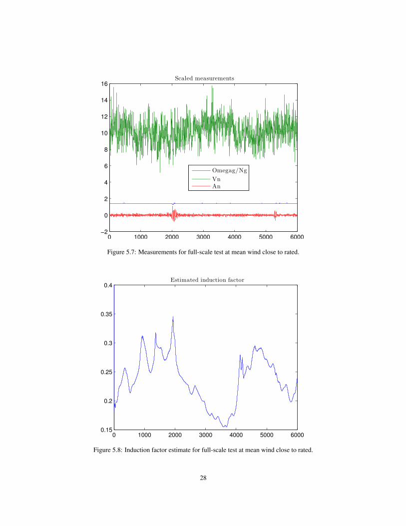
The next data is close to rated wind speed as seen in figure 5.6 where the pitch is active all the time andthere is also two time intervals from 300–400 sec. and from 550–600 sec. where the turbine is in pitchspeed control operation mode. Again the estimated induction factor in figure 5.8 is hard to verify but atleast it is low when the pitch is high.

Again the residuals are far from white as seen in figure 5.9–5.10. The wind measurements residual isagain mostly of low pass type. The peaks from 3P and above which were seen in low wind are also seenhere. The FT and 1P frequencies almost coincides for this wind speed. This means that the 1P probablygives sideways tower movements which can affect the generator speed measurements which again mightcarry over to the pitch via the speed controller. The unmodeled 1P disturbance in the generator speed canalso simply spread via the Kalman gain to the other state estimates. This is a possible explanation forthe large peak at FT/1P for both the speed and acceleration measurements. Then there is also a slowerfrequency peak around 0.2 which is difficult to explain.

Changing the covariances in the KF will change the behavior and potentially improve the performance.There is to many parameters to use trial and error approach for all of them. Therefore the rationale used is

26

−3 −2 −1 1PT 3P 0 DT 1 10

−5

10−4

10−3

10−2

10−1

100

101

102

Log frequency

Magnitude(abs)

Predictions errors

OmegagVnAn

Figure 5.5: Residual spectrum for the full-scale test at mean wind below rated. Notice the extra tickmarks for 1P, first tower (FT), 3P and drive train (DT) frequencies. 1P and FT are close together.

0 1000 2000 3000 4000 5000 6000−3

−2

−1

0

1

2

3

4

5

6

7

Scaled Input

PitchPGen

Figure 5.6: Input for full-scale test at mean wind close to rated.

27

0 1000 2000 3000 4000 5000 6000−2

0

2

4

6

8

10

12

14

16

Scaled measurements

Omegag/Ng

VnAn

Figure 5.7: Measurements for full-scale test at mean wind close to rated.

0 1000 2000 3000 4000 5000 60000.15

0.2

0.25

0.3

0.35

0.4

Estimated induction factor

Figure 5.8: Induction factor estimate for full-scale test at mean wind close to rated.

28

0 20 40−1

0

1

lag

nobs= 5400, p= 0

−50 0 50−0.1

0

0.1

lag

nobs= 5400

−50 0 50−0.5

0

0.5

lag

nobs= 5400

0 20 40−1

0

1

lag

nobs= 5400, p= 0

−50 0 50−0.1

0

0.1

lag

nobs= 5400

0 20 40−1

0

1

lag

nobs= 5400, p= 0

Figure 5.9: Residual test for the full-scale test at mean wind close to rated.

−3 −2 −1 1PT 3P 0 DT 1 10

−5

10−4

10−3

10−2

10−1

100

101

102

Log frequency

Magnitude(abs)

Predictions errors

OmegagVnAn

Figure 5.10: Residual spectrum for the full-scale test at mean wind close to rated. Notice the extra tickmarks for 1P, first tower (FT), 3P and drive train (DT) frequencies. 1P and FT are close together.

29

to keep the process noise, i.e. wind part, covariances fixed. Also the measurements covariance for nacellewind speed and acceleration has mostly been fixed. The generator speed measurements are consideredas the prime measurement with the highest quality. If the speed covariance is increased compared to theabove results the residuals spectrum peaks reduces but becomes more low frequent and larger. If it isdecreased especially the 3P peak increases and also divergence can occur.

5.5 Discussion

It has not so far been possible to point to a few specific reasons for the non white residuals. There are atleast the following many possibilities.

• The non-linearities are to large for the UKF to work. This is probably not very lightly.

• Problems with the parameters

– Cp and Ct tables are with a perhaps to crude resolution which is 2 degrees for pitch and 0.5for tip speed ratios. E.g. 0.5 for pitch and 0.1 for tip speed ratios would be better.

– Tower frequency has already been corrected.

– Rotor and generator inertia and similar "physical" parameters should be correct as they arenot to difficult to measure/calculate.

• Problems with the current model structure.

– The dynamic inflow part may not match reality.

– The rest is very standard.

• Importance of what is left out from the model

– 3P is clearly given errors when covariance on generator speed measurement is small.

– Variations in efficiency for gear and generator and especially air density will be significant.When power, pitch and speed are considered very accurate then this unmodeled uncertaintyends up in the wind state. However, the relative error in wind speed will be approximately1/3 of the error in power e.g. for 25% error 3

√1.25 = 1.077.

NREL Investigation: For NREL 5MW the effect of 10% to high air density has been tested.This increases the predicted state error rms by a factor of 3 for tower movement and 16 forthe induction state while the other states where not affected. Notice that for both states theerror is entirely a offset so maybe it is not to important for fatigue and control. The effect of10% to low air density is similar.

– Blades are not in the model. This is maybe why there is 3 peaks in the spectra for thegenerator speed at approximately 2, 2.1 and 3. The blade frequencies are presently unknown.

• Problems with low observability which maybe also present in the NREL 5MW test in section 4.This is considered to be a less significant problem compared to the above.

Further work based on the above could be.

• Improve resolution of Cp and Ct tables.

• Check other parameters once more.

30

• Use the un-transformed wind speed measurement.

• Include 1P and 3P effects in the model.

• Low pass filter measurement with cut off frequency close to 2 to get rid of higher order unmodeleddynamics from blades etc.

• Include a state for estimating air density or “total efficiency” and perhaps also

• Include measurement uncertainty for pitch and power.

• Investigate problems with colored residuals in the simulated case when the feedback is active.

31

Chapter 6

Conclusion

The main objective with this project is to test if a simple dynamic inflow model will improve the stateestimation for a real commercial wind turbine. For this a successful development and test of a continuousdiscrete version of the unscented Kalman filter has been developed and tested. Test based on simulationsusing NREL5MW virtual turbine was also successful with no or low pitch activity. For high winds withpitch activity all the time the whiteness and other performance of the UKF degraded compared to theideal for linear systems. This has not been explained so far. Test based on data from a real turbineshows that the estimator works and gives reasonably estimates but the residuals are far from white andimprovements should be pursued. A number of potential improvements are suggested. Unfortunately theproject can not be continued as planed in 2014 do to administrative changes. Therefore a final conclusioncan not be given.

32

Bibliography

T. Burton, D. Sharpe, N. Jenkins, and E. Bossanyi. Wind Energy Handbook. John Wiley, 2008.

S. J. Julier, J. K. Uhlmann, and H. F. Durrant-Whyte. A new approach for filtering nonlinear systems. InACC 1995, Seattle, pages 1628–1632, 1995.

T. Knudsen and T. Bak. Simple model for describing and estimating wind turbine dynamic inflow. In2013 American Control Conference, June 17 - 19, Washington, DC., pages 640–646. AACC, IFAC,2013.

T. Knudsen, M. Soltani, and T. Bak. Prediction models for wind speed at turbine locations in a wind farm.Wind Energy, 14:877–894, 2011. Published online in Wiley Online Library (wileyonlinelibrary.com).DOI: 10.1002/we.491.

I. Munteanu, A. I. Bratcu, N.-A. Cutululis, and E. Ceanga. Optimal Control of Wind Energy Systems.Springer, 2008.

S. Thrun, W. Burgard, and D. Fox. Probabilistic Robotics. The MIT Press, 2006.

33

Appendix A

Measurement specifications

To estimate effective wind speed (EWS), at least generator speed, generator power and blade pitch areneeded. This will only be sufficient for sampling and averaging times of more than 1 sec. For control rel-evant modelling with sampling of 0.1 sec. or less many more signals are needed to include the necessarydynamics.

The ideal measurements specifications are shown in table A.1. However, data that do not fully complycan still be very valuable. The specific turbine type and size and whether it is off or onshore have lesspriority as long as it is a pitch to feather type.

The most interesting operating condition is around rated power where the effect of dynamic inflow ismost pronounced. It will be very valuable to have data with forced pitch excitation e.g. in square wavestepping signals of 1-3 degrees and with periods of 100-200 sec. This can be done without disturbing thewind turbine operation much just below rated power when the normal pitch controller is not active. Infull load it is still possible to ad a pitch disturbance but the full load pitch controller must then be allowedto remove this disturbance again. Another possibility will be to use power reference changes to inducethe pitch changes when in full load operation.

34

General Sample time:0.1 sec.Averaging time: samplingt timeDate / Time stamp: absolute

Wind turbine Electrical power producedElectrical power reference (if available)Status signalBlade pitch angles (3)Generator speedRotor speed (if available)Wind speed at turbineWind direction at turbineNacelle directionTower acceleration fore aft and sideways

Meteo mast (if available) Wind speed at 0.5, 1 and 1.5 hub heightWind direction at hub heightTemperature at 0.5, 1 and 1.5 hub height

Conditions Forced pitch excitation in partial load if possibleFour wind speeds:(1) near cut-in,(2) halfway nominal power,(3) near nominal power,(4) high wind speed

Misc Several (10) sets per wind speedAt least 10 min. of data per set preferable longer.

Table A.1: Measurement specification

35

Appendix B

Parameter specifications

To estimate EWS with fast sampling e.g. 0.1 sec. all the below parameters in table B.1 are necessary.

Aerodynamics CP and CT tables for the hole operating range of pitch and tip speed ratioDrive train Slow side (rotor) inertia

Fast side (generator) inertiaSpring constant and damping coefficient orEigen frequency and damping

Generator Losses e.g. viscous damping coefficient and zero load lossesTower Total top inertia

Spring constant and damping coefficient orEigen frequency and damping

Table B.1: Turbine parameter specification

36

Appendix C

Second order statistics for y = xTx forx Gaussian

The objective it this section is to find a test case for testing the unscented transform in section 2.3 wherethe exact theoretical result is known even though the relation is non linear. This is possible for the aboverelation as demonstrated below.

Assume the n dimensional vector x is defined by: covariance

x ∈ N(µx, Cx)⇒ (by definition) E(x) = µx , Cov(x) = Cx , x Gaussian . (C.1)

The problem is then to find E(y),Cov(y),Cov(y, x).

An more useful representation of x is:

x = µx + C12x e , e ∈ N(0, I) (C.2)

where

C12x = UL

12 , U, L are eigen vector and value matrices⇒ (C.3)

C12x C

12x

T

= UL12 (UL

12 )T == UL

12L

12UT = ULUT = Cx , (C.4)

C12x

T

C12x = (UL

12 )TUL

12 == L

12UTUL

12 = L

12L

12 = L (C.5)

Below the following facts about normalised Gaussian variables are used.

e ∈ N(0, I)⇒ (C.6)

E(ei) = 0 , E(e2i ) = 1 , E(e3i ) = 0 , E(e4i ) = Var(e2i ) + E(e2i )2 = 2 + 1 = 3 (C.7)

37

The mean E(y) can then be found as follows:

E(y) = E(xTx)

= E((µx + C12x e)

T(µx + C12x e))

= µTxµx + E((C12x e)

TC12x e)

= µTxµx + E(eTC12x

T

C12x e)

= µTxµx + E(eTLe)

= µTxµx + trace(L)

= µTxµx + trace(Cx)

(C.8)

The cross covariance Cov(y, x) is found in a similar way where we use E(e) = 0 , E(eeT) =I , E(eTAeeTB) = 0 ∀A,B.

Cov(y, x) = E((y − µy)(x− µx)T

)= E

((xTx− µy)(C

12x e)

T)

= E(

(xTx)(C12x e)

T)

= E(

(µx + C12x e)

T(µx + C12x e)(C

12x e)

T)

= E((µTxµx + µTxC

12x e+ (C

12x e)

Tµx + (C12x e)

TC12x e)

(C12x e)

T)

= E((µTxC

12x e+ (C

12x e)

Tµx

)(C

12x e)

T)

= E((

2µTxC12x e)

(C12x e)

T)

= 2µTxC12x E

(eeT)C

12x

T

= 2µTxCx

(C.9)

Finally E(y2) is derived.

E(y2) = E((xTx)2)

= E

(((µx + C

12x e)

T(µx + C12x e))2)

= E

((µTxµx + µTxC

12x e+ (C

12x e)

Tµx + (C12x e)

TC12x e)2)

= E

((µTxµx + 2µTxC

12x e+ eTLe

)2)= (µTxµx)2 + 2µTxµx trace(L) + 4µTxCxµx + E

((eTLe

)2)(C.10)

38

E((eTLe

)2)= E

( n∑i=1

lie2i

)2

= E

n∑i=1

n∑j=1

lilje2i e

2j

= 3

∑i=1

l2i +

n∑i=1

∑j 6=i

lilj

= 2∑i=1

l2i +

n∑i=1

n∑j=1

lilj

(C.11)

The covariance, or variance as it is a scalar, for y is

Cov(y) = Var(y) = E(y2)− E(y)2

= (µTxµx)2 + 2µTxµx trace(Cx) + 4µTxCxµx + 2∑i=1

l2i +

n∑i=1

n∑j=1

lilj

− (µTxµx + trace(Cx))2

= 4µTxCxµx + 2∑i=1

l2i

(C.12)

39

Appendix D

Detailed dynamic model

The EKF is based on a state space model. For convenience all the needed equations are collected in(D.1) starting with the state dynamics and ending with the static relations. The extension compared tothe model used in Knudsen and Bak [2013] are the use of two inertias for the drive train compared toone in the previous work. Please see Knudsen and Bak [2013] for more details.

Irωr = Tr − kdφ− ddφ , (D.1a)

Igωg = (kdφ+ ddφ)1

N− Tg , (D.1b)

φ = ωr − ωg1

N, (D.1c)

Mndn = Fr − ktdn − dtdn , (D.1d)vt = −γ(vm)vt + n1 , (D.1e)vm = n2 , (D.1f)af = κ(vm)(as − af ) , (D.1g)

κ(vm) =2vm3D

, (D.1h)

γ(vm) =πvm2L

, (D.1i)

V1(vm) =πv3mt

2i

L, (D.1j)

vr = vt + vm − dn , (D.1k)

vf = vr1− af1− as

, (D.1l)

as =1

2

(1−

√1− Ct(λ, β)

), (D.1m)

Tr =1

2ρv3fArCp(λ, β)

1

ωr, (D.1n)

Fr =1

2ρv2fArCt(λ, β) , (D.1o)

λ =ωrRrvr

, (D.1p)

40

Tg =p

µωr. (D.1q)

The mechanical part is quite standard and are discussed in several text books [Burton et al., 2008,Munteanu et al., 2008].

The wind model is important for the estimator and is not standard. It is however well described inKnudsen et al. [2011].

The DI inflow part (D.1g), (D.1l) and (D.1m) is new while the rest of the aerodynamics (D.1n)– (D.1p)is standard except that the fictive wind vf is used for rotor torque and thrust.

The measurement part (D.2) simply adds white measurement noise to the rotor speed ωr, the wind speedseen by the nacelle vr and the nacelle acceleration an.

ωm = ωr + v1 , (D.2a)vn = vr + v2 , (D.2b)am = an + v3 . (D.2c)

The state space model with state, input and output is given below in condensed form.

x =[ωr ωg φ dn dn vt vm af

]T, (D.3)

u =[β p

]T, (D.4)

y =[ωm vn am

]T(D.5)

41