Aalborg Universitet The Application of Vector Fitting to ...

Aalborg Universitet

The Application of Vector Fitting to Eigenvalue-based Harmonic Stability Analysis

Dowlatabadi, Mohammadkazem Bakhshizadeh; Yoon, Changwoo; Hjerrild, Jesper; Bak,Claus Leth; Kocewiak, ukasz Hubert; Blaabjerg, Frede; Hesselbæk, BoPublished in:I E E E Journal of Emerging and Selected Topics in Power Electronics

DOI (link to publication from Publisher):10.1109/JESTPE.2017.2727503

Publication date:2017

Document VersionAccepted author manuscript, peer reviewed version

Link to publication from Aalborg University

Citation for published version (APA):Dowlatabadi, M. B., Yoon, C., Hjerrild, J., Bak, C. L., Kocewiak, . H., Blaabjerg, F., & Hesselbæk, B. (2017). TheApplication of Vector Fitting to Eigenvalue-based Harmonic Stability Analysis. I E E E Journal of Emerging andSelected Topics in Power Electronics, 5(4), 1487 - 1498. https://doi.org/10.1109/JESTPE.2017.2727503

General rightsCopyright and moral rights for the publications made accessible in the public portal are retained by the authors and/or other copyright ownersand it is a condition of accessing publications that users recognise and abide by the legal requirements associated with these rights.

- Users may download and print one copy of any publication from the public portal for the purpose of private study or research. - You may not further distribute the material or use it for any profit-making activity or commercial gain - You may freely distribute the URL identifying the publication in the public portal -

Take down policyIf you believe that this document breaches copyright please contact us at [email protected] providing details, and we will remove access tothe work immediately and investigate your claim.

Downloaded from vbn.aau.dk on: March 15, 2022

https://doi.org/10.1109/JESTPE.2017.2727503

https://vbn.aau.dk/en/publications/b861f8ba-f5ca-47f8-9cb6-a861be4f08f6

https://doi.org/10.1109/JESTPE.2017.2727503

2168-6777 (c) 2017 IEEE. Personal use is permitted, but republication/redistribution requires IEEE permission. See http://www.ieee.org/publications_standards/publications/rights/index.html for more information.

This article has been accepted for publication in a future issue of this journal, but has not been fully edited. Content may change prior to final publication. Citation information: DOI 10.1109/JESTPE.2017.2727503, IEEE Journalof Emerging and Selected Topics in Power Electronics

1

Abstract— Participation factor analysis is an interesting

feature of the eigenvalue-based stability analysis in a power

system, which enables the developers to identify the problematic

elements in a multi-vendor project like in an offshore wind power

plant. However, this method needs a full state space model of the

elements that is not always possible to have in a competitive

world due to confidentiality. In this paper, by using an

identification method, the state space models for power

converters are extracted from the provided data by the suppliers.

Some uncertainties in the identification process are also discussed

and solutions are proposed, and in the end the results are verified

by time domain simulations for linear and nonlinear cases with

different complexities, no matter which domain (phase or dq) is

used.

Index Terms— Eigenvalue analysis; Harmonic Stability;

Matrix Fitting; Participation Factor Analysis; Vector Fitting

I. INTRODUCTION

HE drastic increasing trend of global energy consumption

and the demand for cleaner and more sustainable energy

are bringing more new and renewable energy sources into the

existing power system [1]–[3]. As a consequence of the very

wide-spread renewable energy resources, the interfacing units,

typically Power Electronics (PE) based power devices, are

connected anywhere in the existing power system and

unexpected interaction problems are caused by these newly

installed PE units [4]–[7]. These interaction problems can be

categorized by their frequency range into two categories. One

is low-frequency small signal instability around the

fundamental frequency [8]–[10] or even lower frequency, such

as the sub-synchronous resonance frequency [11]–[13]. The

other one is the instability with the relatively higher

frequencies ranged from a few hundred Hertz to a few kilo

Hertz [7], [14], [15]. Even though the physical reason of these

Manuscript received February 27, 2017; revised May 15, 2017; accepted

June 27, 2016. This work was supported in part by the DONG Energy Wind

Power A/S and in part by the Innovation Fund Denmark. M. K. Bakhshizadeh, J. Hjerrild, Ł. Kocewiak, and B. Hesselbæk are with

the DONG Energy Wind Power, Fredericia 7000, Denmark (e-mail:

[email protected]; [email protected]; [email protected]; bohes@ dongenergy.dk).

C. Yoon, C. L. Bak, and F. Blaabjerg are with the Department of Energy

Technology, Aalborg University, Aalborg DK-9220, Denmark (e-mail: [email protected]; [email protected]; [email protected]).

instabilities may be different from each other, all these

interaction problems can be understood by the conditions that

creates unstable poles in the system transfer-function [16],

[17].

There are typically two ways to assess small signal stability.

One is the Impedance Based Stability Analysis (IBSA) [17]

and the other one is the eigenvalue-based analysis using the

State-Space (SS) model [16]. The IBSA evaluates the system’s

stability using the ratio of the impedance of the two sub

systems (lumped impedances) that are connected to the node

under study. While the eigenvalue-based method models the

entire system as SS matrices, the IBSA is a simpler method

but gives only local information about the stability of the

system. The IBSA is confined only to an interconnection point

and it needs to be remodeled repeatedly in order to assess

somewhere else [18], [19]. In contrast SS models are harder to

get but using them one can study the system globally. The SS

model allows the participation factor analysis or the sensitivity

analysis [20], [21] which is very necessary when imposing a

responsibility of the interaction problem to the participants in

the power network. Phenomenally, the interaction problem is a

compounded issue with the linked impedances and the

participant can be an offender or a victim at the same time. In

that sense, it is necessary to have a quantitative method that

measures the effect on the poles of the entire system

(eigenvalues) from varying the state variables in each

subsystem [20]. The entire SS model can be found using a

systematic and modular method called Component Connection

Method (CCM) [22], [23]. Also, by the help of CCM, the

problematic state variables in each subsystem can be managed

and visible easily [21].

However, this method is only possible on the assumption

that we have proper SS models of all subsystems. The problem

is with the confidentiality of the commercial products where

the detailed SS model cannot be obtained and can only be

reconstructed indirectly such as by Vector Fitting (VF) [24]–

[26]. In [27] the application of the VF in eigenvalue-based

stability analysis has been introduced, in which based on

measurements from a node in the network, an SS model is

proposed using the VF. However, since this model is based on

a local measurement, the model is local and not global. In

other words, it cannot show the dynamics of the entire system

if there are some symmetries in the system, which leads to the

appearance of some hidden dynamics [28], and as a result this

The Application of Vector Fitting to

Eigenvalue-based Harmonic Stability Analysis

Mohammad Kazem Bakhshizadeh, Student Member, IEEE, Changwoo Yoon, Student Member, IEEE,

Jesper Hjerrild, Claus Leth Bak, Senior Member, IEEE, Łukasz Kocewiak, Senior Member, IEEE,

Frede Blaabjerg, Fellow, IEEE, and Bo Hesselbæk

T



2

method must be repeated at different nodes. It also needs a

stable system to do measurements, because if the system is

unstable, then no measurement can be done and this method is

not applicable. Finally, since the entire network is modelled as

a black box seen from the measurement point, no further

studies such as the participation factor analysis can be done to

find the most problematic component in a system. It must be

noted that the method proposed in this paper can be

considered as an extension to [27] when more information is

available.

In this paper, system stability analysis based on SS and

CCM by using the indirect VF is presented. Some interaction

case examples are adopted to show the validity of this

procedure. The result shows that the problematic subsystem

could be identified based on the participation factor analysis

even for an unstable system. Since the method models the

entire system using a systematic approach, it includes all

dynamics of the system. Some uncertainties in the VF are also

discussed.

II. EIGENVALUE ANALYSIS

A. Stability Evaluation

If one has the overall SS representation of a system, for

instance as given in (1), then the stability can be evaluated by

investigating the eigenvalues of matrix A, which is called the

state (or system) matrix [29]. The eigenvalues are indeed poles

of the system and if their real part is positive, then the system

is unstable. It must be noted that in this paper the focus is on

linear/linearized SS models.

�̇� = 𝐴𝑥 + 𝐵𝑢 𝑦 = 𝐶𝑥 + 𝐷𝑢

(1)

The eigenvalues also contain some other useful information

[20], for instance if the ith

eigenvalue/pole, which is called

hereafter the ith

mode, is

𝜆𝑖 = 𝜎𝑖 + 𝑗𝜔𝑖 (2)

Then the oscillation frequency of that mode is ωi, the time

constant of that mode, very similar to a first order RC system,

is 1/σi and the damping is defined as

𝜉𝑖 = −𝜎𝑖

√𝜎𝑖2 + 𝜔𝑖

2 (3)

In other words the transient response of the system to a

perturbation includes this frequency which will decay with the

specified time constant/damping. A negative damping by

definition indicates an unstable case, where instead of

damping, amplifying happens. Therefore, not only the stability

of the system can be assessed using the sign of the real parts,

but also the minimum damping of the system can be found.

The latter can be considered as a measure that states how

stable a system is.

B. How to find the overall SS model

One problem is how to find the SS representation of such a

complicated system, which has some controllers in addition to

a coupled electrical system. The Component Connection

Method (CCM) is a good way to deal with very complicated

systems [23]. In this method each subsystem (power

converters, passive network and etc.) is modelled separately

and in the end the overall SS can be found by some simple

matrix operations. Modelling the system in this way is much

easier and the equations are more readable. The

implementation of this algorithm in a computer program is

also more straightforward. In this method, first the block

diagonal matrices are created by simply appending the

different SS matrices individually without considering the

interconnections between them.

𝑥�̇� = 𝐴𝑖𝑥𝑖 + 𝐵𝑖𝑢𝑖 𝑦𝑖 = 𝐶𝑖𝑥𝑖 + 𝐷𝑖𝑢𝑖

(4)

𝐴𝑎𝑝𝑝 = [

𝐴1 0 … 00 𝐴2 … ⋮⋮ ⋮ ⋱ 00 … 0 𝐴𝑛

] , 𝑥𝑎𝑝𝑝 = [

𝑥1

𝑥2

⋮𝑥𝑛

] (5)

𝐵𝑎𝑝𝑝 = [

𝐵1 0 … 00 𝐵2 … ⋮⋮ ⋮ ⋱ 00 … 0 𝐵𝑛

] , 𝑢𝑎𝑝𝑝 = [

𝑢1

𝑢2

⋮𝑢𝑛

] (6)

𝐶𝑎𝑝𝑝 = [

𝐶1 0 … 00 𝐶2 … ⋮⋮ ⋮ ⋱ 00 … 0 𝐶𝑛

] , 𝑦𝑇 = [

𝑦1

𝑦2

⋮𝑦𝑛

] (7)

𝐷𝑎𝑝𝑝 = [

𝐷1 0 … 00 𝐷2 … ⋮⋮ ⋮ ⋱ 00 … 0 𝐷𝑛

] (8)

Then, the final matrices can be obtained by

𝑢𝑐𝑚𝑝 = 𝐿1𝑦𝑐𝑚𝑝 + 𝐿2𝑢𝑠𝑦𝑠 (9)

𝑦𝑠𝑦𝑠 = 𝐿3𝑦𝑐𝑚𝑝 + 𝐿4𝑢𝑠𝑦𝑠

where, L1 to L4 , which are called the interconnection

matrices, are the matrices which define the relationship

between the inputs and outputs of the individual components

(ucmp and ycmp) and the inputs and outputs of the total system

(usys and ysys). The total SS model is described by

�̇�𝑎𝑝𝑝 = 𝐴𝑇𝑥𝑎𝑝𝑝 + 𝐵𝑇𝑢𝑠𝑦𝑠

𝑦𝑠𝑦𝑠 = 𝐶𝑇𝑥𝑎𝑝𝑝 + 𝐷𝑇𝑢𝑠𝑦𝑠 (10)

where,

𝐴𝑇 = 𝐴𝑎𝑝𝑝 + 𝐵𝑎𝑝𝑝𝐿1(𝐼 − 𝐷𝑎𝑝𝑝𝐿1)−1

𝐶𝑎𝑝𝑝

(11) 𝐵𝑇 = 𝐵𝑎𝑝𝑝𝐿1(𝐼 − 𝐷𝑎𝑝𝑝𝐿1)

−1𝐷𝑎𝑝𝑝𝐿2 + 𝐵𝑎𝑝𝑝𝐿2

𝐶𝑇 = 𝐿3(𝐼 − 𝐷𝑎𝑝𝑝𝐿1)−1

𝐶𝑎𝑝𝑝

𝐷𝑇 = 𝐿3(𝐼 − 𝐷𝑎𝑝𝑝𝐿1)−1

𝐷𝑎𝑝𝑝𝐿2 + 𝐿4

and I is the identity matrix.

C. Improper transfer functions

A transfer function is called improper, if the order of the

numerator polynomial is more than the order of the

denominator polynomial. The SS model of an improper

transfer function could not be described by only A, B, C and D



3

matrices and another matrix E is needed to model the extra

order.

�̇� = 𝐴𝑥 + 𝐵𝑢𝑦 = 𝐶𝑥 + 𝐷𝑢 + 𝐸�̇�

(12)

The VF is able to find the E matrix; however, in this paper

the improper transfer functions are avoided by choosing a

proper impedance or admittance representation. For instance,

for Current-Controlled Converters (such as solar inverters) a

series inductor is normally used for smoothing the output

current, therefore this series inductance makes the transfer

function of the output impedance improper. However, by

using the admittance model for a current controlled converter

this problem can be avoided. The same can be concluded for

Voltage-Controlled Converters, in which a capacitive shunt is

used at the output terminal. Thus, for a Voltage-Controlled

Converter an impedance model should be used. As a

conclusion the E matrix is not necessary in the identification

process by choosing the correct models based on the

application and a little engineering judgement. If the

magnitude of the frequency response goes up for higher

frequencies, then it means the current model might be

improper.

III. THE PROPOSED METHOD FOR DEALING WITH BLACK BOX

MODELS

If the SS models of converters and other elements are

available, then one can use the aforementioned method and

evaluate the stability. However, the structure and parameters

of the power converters are not always available due to

confidentiality and intellectual property rights. Instead, the

terminal characteristics of the converter are delivered as a look

up table, which shows the frequency response of the converter

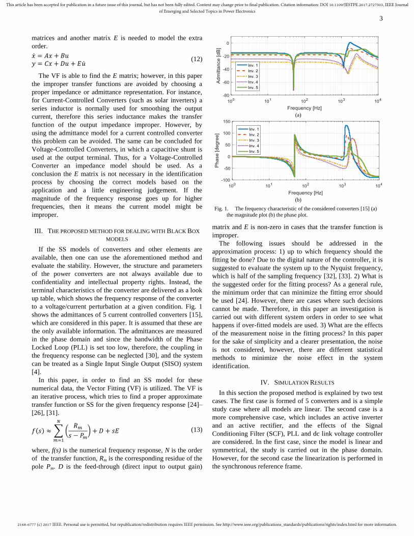
to a voltage/current perturbation at a given condition. Fig. 1

shows the admittances of 5 current controlled converters [15],

which are considered in this paper. It is assumed that these are

the only available information. The admittances are measured

in the phase domain and since the bandwidth of the Phase

Locked Loop (PLL) is set too low, therefore, the coupling in

the frequency response can be neglected [30], and the system

can be treated as a Single Input Single Output (SISO) system

[4].

In this paper, in order to find an SS model for these

numerical data, the Vector Fitting (VF) is utilized. The VF is

an iterative process, which tries to find a proper approximate

transfer function or SS for the given frequency response [24]–

[26], [31].

𝑓(𝑠) ≈ ∑ (𝑅𝑚

𝑠 − 𝑃𝑚

)

𝑁

𝑚=1

+ 𝐷 + 𝑠𝐸 (13)

where, f(s) is the numerical frequency response, N is the order

of the transfer function, Rm is the corresponding residue of the

pole Pm. D is the feed-through (direct input to output gain)

matrix and E is non-zero in cases that the transfer function is

improper.

The following issues should be addressed in the

approximation process: 1) up to which frequency should the

fitting be done? Due to the digital nature of the controller, it is

suggested to evaluate the system up to the Nyquist frequency,

which is half of the sampling frequency [32], [33]. 2) What is

the suggested order for the fitting process? As a general rule,

the minimum order that can minimize the fitting error should

be used [24]. However, there are cases where such decisions

cannot be made. Therefore, in this paper an investigation is

carried out with different system orders in order to see what

happens if over-fitted models are used. 3) What are the effects

of the measurement noise in the fitting process? In this paper

for the sake of simplicity and a clearer presentation, the noise

is not considered, however, there are different statistical

methods to minimize the noise effect in the system

identification.

IV. SIMULATION RESULTS

In this section the proposed method is explained by two test

cases. The first case is formed of 5 converters and is a simple

study case where all models are linear. The second case is a

more comprehensive case, which includes an active inverter

and an active rectifier, and the effects of the Signal

Conditioning Filter (SCF), PLL and dc link voltage controller

are considered. In the first case, since the model is linear and

symmetrical, the study is carried out in the phase domain.

However, for the second case the linearization is performed in

the synchronous reference frame.

(a)

(b)

Fig. 1. The frequency characteristic of the considered converters [15] (a)

the magnitude plot (b) the phase plot.



4

Inv. 5

Inv. 4

Inv. 3

Inv. 2

CPFC

RS

LS

vg

PCC

Inv. 1vdc

ig

iinv1

iinv5

(a)

αβ

PWM

abc

12

num

den

÷Limiter

KI s

s2+ω02

KP

PLL

ω0 θ

iINV

αβ

abc

iαβ

iαβ

vdc

ω0

Lf Lg

Cf

Rd

vMvPCC

i*αβ

vdc

rLf rLg

rCf

(b)

Fig. 2. The considered power system [15], which is based on Cigré LV

benchmark system [34]: a) the overall power scheme. (b) the

converter internal control structure.

TABLE I. THE PARAMETERS OF THE CONSIDERED POWER SYSTEM

[15].

Symbol / Description Inverters

1 2 3 4 5

fsw Switching/Sampling frequency [kHz]

10 16 10

Vdc DC-link voltage [V] 750

Lf Inverter side inductor

of the filter [mH] 0.87 1.2 5.1 3.8 0.8

Cf Filter capacitor [μF] 22 15 2 3 15

Lg Grid side inductor of

the filter [mH] 0.22 0.3 1.7 1.3 0.2

rLf Parasitic resistance of

Lf [mΩ] 11.4 15.7 66.8 49.7 10

rCf Parasitic resistance of

Cf [mΩ] 7.5 11 21.5 14.5 11

rLg Parasitic resistance of

Lg [mΩ] 2.9 3.9 22.3 17 2.5

Rd Damping resistance

[Ω] 0.2 1.4 7 4.2 0.9

Kp Proportional gain of

the controller 5.6 8.05 28.8 16.6 6.5

Ki Integrator gain of the

controller 1000 1500 1000

Ls Grid inductance [mH] 0.4

Rs Grid resistance [Ω] 0.1

TABLE II. DIFFERENT CONFIGURATIONS OF 0AND THE

CORRESPONDING RESULTS [15]

Case No. Description Result

1 All are connected Stable

2 Inverter 5 is disconnected Unstable

3 Inverter 2 is disconnected Unstable

4 Inverter 3 is disconnected Stable

5 Inverter 3 and 4 are disconnected Stable

A. A Linear Case study

Fig. 2 shows the considered power system, which is based

on to the Cigré LV benchmark system [34]. The current

control is done using a Proportional Resonant controller as

shown in Fig. 2, and the parameters of the electrical system

and controllers are listed in Table I. Depending on which

converters are connected or disconnected, different stable and

unstable cases can be seen [15], [35]. Table II shows a few

different configurations and Fig. 3 is the time domain

simulation considering those cases.

Fig. 4 shows the magnitude plot of the admittance of

Inverter 2 and the accuracy of the identified models

(magnitude of the absolute error) with 6th, 8th and 12th orders

by the VF. It must be noted that since the original admittance

plots are results of a measurement, therefore, they must model

a stable system. To ensure that no Right Half Plane (RHP)

pole appears in the identified models, the stability enforcement

must be used, which simply rejects unstable poles in each

iteration. For elements where the transfer function is

accessible, one can find the equivalent SS representation. For

instance, the SS equations of the network can directly be

obtained from the differential equations describing the system

dynamics (notice the notations and directions in Fig. 2) as (14)

and (15).

Fig. 5 shows the considered power system as a control

block diagram in order to show how CCM can be utilized. The

L1, L2, L3 and L4 interconnection matrices of (9) and (11) are

given as (16). The inputs and outputs are highlighted with red

and blue signals, respectively. The elements of ucmp and ycmp

0 0.05 0.1 0.15 0.2 0.25 0.3 0.35 0.4-0.1

-0.05

0

0.05

0.1

Curr

ent[

kA]

Time [sec]

Inv.1 Inv.2 Inv.3 Inv.4 Inv.5

Case 1 Case 2 Case 1 Case 3 Case 1 Case 4 Case 5

Fig. 3. Time domain simulations for different cases [15] shown in Table II.



5

vectors are also highlighted in the Fig. 5. Any signal can be

considered as the system input and output, however as an

example, the grid voltage vg is considered as the input to the

overall system and vpcc is considered as the output.

𝐿1 = [

[0]5×5 [1]5×1

0 0[𝐼]5×5 [0]5×1

] , 𝐿2 = [[1]5×1

[0]6×1]

(16)

𝐿3 = [[0]1×5 1], 𝐿4 = [0]

1) Challenges in the VF

The CCM as described above can be utilized to build up the

entire SS model of the system and to study the system

dynamics [23]. Fig. 6 shows the pole plot of the entire system

(for Case 5) for different identification orders that is zoomed

in for a better view and the reader cannot see all the high

frequency poles. Time domain simulations for a detailed

switching model as shown in Fig. 3 indicate the stable

operation of Case 5. However, there are some RHP poles in

the identified system as listed in Table III.

One may think that the unstable identified poles are caused

by overfitting, because the unstable poles do not appear for the

6th

order, but the problem is indeed caused by the lack of

information for the frequencies beyond the trained range of the

frequency. Fig. 7 shows the sum of admittances of the

converters for Case 5 (Y1+Y2+Y5) for the original data and the

fitted data with different orders. It can be seen that at the high

frequency range, beyond the trained range, there is a non-

passive region, which causes those unstable poles reported

in TABLE III for the 8th

order model. Actually, this is the

reason why passivity enforcement is necessary in the VF.

Passivity enforcement is the process during the VF to make

sure that the model is passive at all frequencies even beyond

the trained range [36]. This can be done by enforcing the

Hamiltonian matrix of the identified system to have no

imaginary eigenvalues [37]. Passivity enforcement is

necessary in approximating the passive elements such as

transformers, because the models will afterwards be used in

time domain simulations and if they are non-passive, they

might make the system unstable. However, this is not a

𝐶𝑃𝐹𝐶

𝑑

𝑑𝑡𝑣𝑝𝑐𝑐 + 𝑖𝑔 = 𝑖𝑖𝑛𝑣1 + 𝑖𝑖𝑛𝑣2 + 𝑖𝑖𝑛𝑣3 + 𝑖𝑖𝑛𝑣4 + 𝑖𝑖𝑛𝑣5

𝑣𝑝𝑐𝑐 = 𝐿𝑠

𝑑

𝑑𝑡𝑖𝑔 + 𝑅𝑠𝑖𝑔 + 𝑣𝑔

(14)

�̇� = 𝐴𝑛𝑒𝑡𝑥 + 𝐵𝑛𝑒𝑡𝑢 =

[ −

𝑅𝑠

𝐿𝑠

1

𝐿𝑠

−1

𝐶𝑃𝐹𝐶

0]

[𝑖𝑔

𝑣𝑝𝑐𝑐] +

[ −

1

𝐿𝑠

0 0 0 0 0

01

𝐶𝑃𝐹𝐶

1

𝐶𝑃𝐹𝐶

1

𝐶𝑃𝐹𝐶

1

𝐶𝑃𝐹𝐶

1

𝐶𝑃𝐹𝐶]

[

𝑣𝑔

𝑖𝑖𝑛𝑣1

𝑖𝑖𝑛𝑣2

𝑖𝑖𝑛𝑣3

𝑖𝑖𝑛𝑣4

𝑖𝑖𝑛𝑣5]

𝑦 = [𝑣𝑝𝑐𝑐] = 𝐶𝑛𝑒𝑡𝑥 + 𝐷𝑛𝑒𝑡𝑢 = [0 1]𝑥 + [0 0 0 0 0 0]𝑢

(15)

Fig. 4. The original data (admittance of Inverter 2) and the fitting errors

for different fitting orders.

vPCC

-Yinv1

-Yinv3

-Yinv5

Grid

model

vgivsi1

ivsi3

ivsi5

cmp1

cmp3

cmp5

cmp6

ucmp[1]

ucmp[3]

ucmp[5]

ucmp[7]

ucmp[9]

ucmp[11]

ucmp[6]ycmp[1]

ycmp[3]

ycmp[5]

ycmp[6]

usys

ysys

Fig. 5. The considered power system in Fig. 2 as a control block diagram.

Fig. 6. The pole plot of the entire system (as shown in Fig. 2) for Case 5.

TABLE III. THE UNSTABLE POLES OF THE SYSTEM SHOWN IN 0

Unstable poles depending on the order [s-1]

6th 8th 12th

- 1.04e7 1.69e6

- 0.88e7 4.46e4±j1.56e5



6

concern in this study, because: 1) the aim of this paper is not

to develop a model for time domain simulations, in fact

evaluating the stability is the target here. 2) a power converter

is not a passive component due to [33]: a) the time delay,

computational and PWM delay which affect the high

frequency region b) The current controller which affects the

current control bandwidth (for example a Constant Power

Load introduces a negative resistance in the control

bandwidth) c) The low frequency outer loop controllers (e.g.

PLL, voltage and power controller), which affect the low

frequency range.

Therefore, the passivity enforcement is not applicable for

power converter approximation. The proposed workaround in

this paper is to limit the frequency of the identified poles of

the total system. In other words the system is trained up to 10

kHz, therefore, the identified poles beyond this range must be

disregarded. It can easily be done by removing the poles,

which are outside the confidence circle as shown in Fig. 8.

2) Participation factor analysis

By removing the high frequency poles from the study, the

Participation Factor (PF) analysis can be done by some simple

matrix operations [20], [21]. For the ith

pole, the participation

analysis can be done using

𝑃𝑘𝑖 =𝜕𝜆𝑖

𝜕𝑎𝑘𝑘

= 𝛷𝑘𝑖𝛹𝑖𝑘 (17)

where, Φ𝑖 is the right eigenvector of the ith

eigenvalue,Ψ𝑖 is the

left eigenvector of the ith

eigenvalue, and Pki indicates the

contribution of the kth

state on the ith

pole.

In this section Case 2, which is unstable, is considered [15],

[35]. It can be seen in Fig. 9 that the instability is due to an

eigenvalue at (229±j8180) rad/s. Table IV shows the five

largest contributors to this unstable pole and also indicates that

despite different approximation orders they identify the

contribution levels to be almost the same. It can be seen that

Inverter 1 has the most contribution to the unstable pole. Since

the model is a black box, no more conclusions can be made on

which part of Inverter 1 is causing the instability. However, by

informing the supplier about this, they can improve the

stability by looking at the frequency of stability.

3) Time domain simulations

As discussed in section II.A, an eigenvalue contains

information about the transient response, i.e. how fast the

transient decays/grows and at which frequency. In this section,

(a)

(b)

Fig. 7. The bode plot of the aggregated admittance of converters for the

original data and the approximated models for Case 5. (a) magnitude plot (b)

phase plot.

Fig. 8. The poles outside of the confidence circle must be disregarded (this

is for Case 5).

Fig. 9. Pole plot of Case 2, where an unstable pole is highlighted.

TABLE IV. THE PARTICPATION FACTOR ANALYSIS FOR CASE 2 THAT IS

UNSTABLE.

6th order 8th order 12th order

State Name PF State Name PF State Name PF INV1.State 3 0.296 INV1.State 4 0.294 INV1.State 5 0.295

INV1.State 4 0.302 INV1.State 5 0.300 INV1.State 6 0.300

INV2.State 3 0.167 INV2.State 3 0.167 INV2.State 7 0.167 INV2.State 4 0.169 INV2.State 4 0.169 INV2.State 7 0.169

Grid.State 1 0.112 Grid.State 1 0.112 Grid.State 1 0.112



7

the previously presented cases are reviewed again by means of

time domain simulations. Simulations are carried out in

PLECS [38] using a very detailed switching model. The

controller is exactly modeled by using triggered subsystems to

mimic the sampled-based control loop in a real DSP. The

single update PWM is used in this paper, which is the reason

the sampling and switching frequencies are equal. The most

critical eigenvalue, which has the lowest damping, in Case 5 is

-64 ± 8254j, which indicates an oscillation frequency of 8254

rad/s and a time constant of -1/64 seconds. It can be seen in

Fig. 10 that the oscillation frequency in Case 5 after a

perturbation is accurately anticipated. The measured time

constant is also roughly correct, since the oscillation

magnitude (peak to peak) is changed -61 % from t1=0.201 to

t2=0.211 [s]. However, a -47% drop is predicted by the

decaying/growing exponential function (18).

𝐼2𝐼1

= 𝑒(𝑡2−𝑡1)/𝜏 (18)

where, τ=1/σ is the time constant (for a stable pole it is

negative), and I2 and I1 are the current magnitudes at t=t2 and

t=t1, respectively.

Similar study is also done for the Case 2, which is unstable.

The unstable eigenvalues are 229±j8180 rad/s. The

highlighted oscillation frequency in Fig. 11 is almost the same

the imaginary part of the predicted eigenvalue. In the

simulation the peak to peak magnitude is changed 962% from

t1=0.203 to t2=0.213 [s], which indicates a good correlation

with the predicted change of 887% using (18).

B. A nonlinear case

Linearized models should be used for small-signal stability

analysis of nonlinear systems. Therefore, the first step in

analyzing the stability using the proposed method is to find the

steady state operating point that can be obtained after a load

flow. In this paper the linearization is performed in a

synchronously rotating frame (the dq frame), where each ac

quantity can be modelled by two dc signals (d- and q-

channels).

In contrast to linear systems, the linearized nonlinear

models are dependent on an operating point, and as shown in

[39], by changing the operating point the

admittance/impedance characteristics would be different.

Therefore, for each condition (e.g. different active and reactive

power generation) a new set of numerical data should be used

for identification. In [39] it has been shown that by some

simple sensitivity studies the admittance/impedance can be

found for any operating point. It should also be noted that

power system elements are mostly operated very close to the

nominal conditions. Therefore, assuming a constant

admittance profile for studies seems reasonable. Furthermore,

it should also be taken into account that providing the correct

data for studies is the suppliers’ responsibility. Therefore, in

this part the given characteristics are for the given operating

point and finding the operating point dependent characteristics

is out of scope of this paper.

Another important point is that the nonlinear behavior in the

power electronic devices mostly happens in the low frequency

range (i.e. less than two times the fundamental frequency) due

to the fact that the outer loop controllers have a bandwidth

much slower than the current controller. Therefore, if the

objective is to study the interactions in the harmonic frequency

range (medium to high frequency), linear models can be used

in a similar way to the previous case, where PLL dynamics are

neglected [4].

Outer loop control (dc link control, power control and

synchronization loop) generally results in an Multi-Input

Multi-Output (MIMO) control system, where the impedance

characteristics cannot be considered as in a SISO system [30],

[40]. In phase (sequence) domain modelling, they result in

appearance of some frequency couplings, i.e. if a small signal

voltage perturbation is applied at the converter terminals, then

the converter will respond with different frequencies. In the

case of a balanced system with a current controller in the dq

frame and a simple SRF PLL, the response includes ωp and

ωp-2ω1 where ωp is the perturbation frequency and ω1 is the

fundamental frequency. Then a 2x2 matrix must be used as the

converter admittance/impedance for small signal stability

analysis. In the dq domain modelling, normally impedances

are defined as 2x2 dq impedances, and since the operating

point is a dc signal (as long as the system is balanced) in the

dq frame the aforementioned frequency couplings do not

happen.

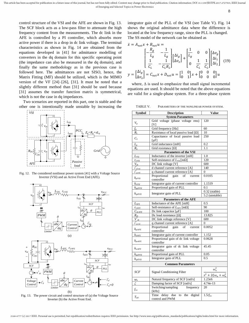
In this section to study the effects of the synchronization

loop (PLL) and the dc link control, a test case as shown in Fig.

12 is considered. The Voltage Source Inverter (VSI) injects

active current to the PCC while the Active Front End (AFE)

feeds a dc load by absorbing active power from the PCC. This

system is based on the test system considered in [41] and the

parameters are listed in Table V. The power circuit and the

Fig. 10. Time domain results for Case 5, where the system remains stable

after a perturbation.

Fig. 11. Time domain results for Case 2, where the system loses stability

after a perturbation.



8

control structure of the VSI and the AFE are shown in Fig. 13.

The SCF block acts as a low-pass filter to attenuate the high

frequency content from the measurements. The dc link in the

AFE is controlled by a PI controller, which absorbs more

active power if there is a drop in dc link voltage. The terminal

characteristics as shown in Fig. 14 are obtained from the

equations developed in [41] for admittance modelling of

converters in the dq domain for this specific operating point

(the impedance can also be measured in the dq domain), and

finally the same methodology as in the previous case is

followed here. The admittances are not SISO, hence, the

Matrix Fitting (MF) should be utilized, which is the MIMO

version of the VF [24]–[26], [31]. It must be noted that a

slightly different method than [31] should be used because

[31] assumes the transfer function matrix is symmetrical,

which is not the case in dq impedances.

Two scenarios are reported in this part, one is stable and the

other one is intentionally made unstable by increasing the

integrator gain of the PLL of the VSI (see Table V). Fig. 14

shows the original admittance data where the difference is

located at the low frequency range, since the PLL is changed.

The SS model of the network can be obtained as

�̇� = 𝐴𝑛𝑒𝑡𝑥 + 𝐵𝑛𝑒𝑡𝑢 =

[ −

𝑅𝑔

𝐿𝑔

−1

𝐿𝑔

1

𝐶𝐿

−1

𝐶𝐿𝑅𝐿]

[∆𝑖𝑔∆𝑣𝑥

] +

[ 1

𝐿𝑔

0 0

01

𝐶𝐿

1

𝐶𝐿]

[

∆𝑣𝑔

∆𝑖1∆𝑖2

]

𝑦 = [∆𝑖𝑔∆𝑣𝑥

] = 𝐶𝑛𝑒𝑡𝑥 + 𝐷𝑛𝑒𝑡𝑢 = [1 00 1

] 𝑥 + [0 0 00 0 0

] 𝑢

(19)

where, Δ is used to emphasize that small signal incremental

equations are used. It should be noted that the above equations

are valid for a single-phase system. For a three-phase system

vdc

vdcRDC Grid

Passive

load

VSI

AFE

Zg=Rg+sLgPCC

ig

iVSI

iAFE

CDC

Fig. 12. The considered nonlinear power system [41] with a Voltage Source Inverter (VSI) and an Active Front End (AFE).

dq

PWM

abc Current

ControlLimiter

PLLθ

iVSI

dq

abc

idq

vdc

LVSIvMvPCC

i*dq

rLVSI

θ

SCF

iabc vabc

(a)

dq

PWM

abc Current

ControlLimiter

PLLθ

iAFE

dq

abc

idq

+

vdc

_

LAFEvMvPCC

rLAFE

θ

SCF

iabc vabc

Voltage

Controli*

d

i*d

i*q=0

SCF

v*dc

RDC

CDC

(b)

Fig. 13. The power circuit and control structure of (a) the Voltage Source Inverter (b) the Active Front End.

TABLE V. PARAMETERS OF THE NONLINEAR POWER SYSTEM.

Symbol Description Value

System Parameters

Vg Grid voltage (phase voltage rms)

[V]

120

fg Grid frequency [Hz] 60

RL Resistance of local passive load [Ω] 10

CL Capacitance of local passive load

[μF]

250

Lg Grid inductance [mH] 0.2

Rg Grid resistance [Ω] 1.1

Parameters of the VSI

LVSI Inductance of the inverter [mH] 1.0

rLVSI Self-resistance of LVSI [mΩ] 120

Vdc DC link voltage [V] 600

i*d-vsi d channel current reference [A] 140

i*q-vsi q channel current reference [A] 0

kpiVSI Proportional gain of current

controller

0.0105

kiiVSI Integrator gain of current controller 1.1519

kppllVSI Proportional gain of PLL 0.1

kipllVSI Integrator gain of PLL 0.32 (stable)

5.2 (unstable)

Parameters of the AFE

LAFE Inductance of the AFE [mH] 0.5

rLAFE Self-resistance of LAFE [mΩ] 90

CdcAFE Dc link capacitor [μF] 100

Rdc Dc load resistance [Ω] 13.825

V*dc DC link voltage reference [V] 600

i*q-vsi q channel current reference [A] 0

kpiAFE Proportional gain of current

controller

0.0052

kiiAFE Integrator gain of current controller 1.152

kpvAFE Proportional gain of dc link voltage

controller

0.0628

kivAFE Integrator gain of dc link voltage

controller

45.45

kppllVSI Proportional gain of PLL 0.05

kipllVSI Integrator gain of PLL 0.5

Common Parameters

SCF Signal Conditioning Filter 𝜔𝑛

2

𝑠2 + 2𝜉𝜔𝑛 + 𝜔𝑛2

ωn Natural frequency of SCF [rad/s] 1.23e6

ξ Damping factor of SCF [rad/s] 4.74e-13

fsw Switching/sampling frequency

[kHz]

20

Tdel Time delay due to the digital control and PWM

1.5/fsw



9

the equations can be transformed into dq domain [42] using

𝐴𝑑𝑞 = [𝐴𝑛𝑒𝑡 −𝜔1𝐼𝜔1𝐼 𝐴𝑛𝑒𝑡

] , 𝐵𝑑𝑞 = [𝐵𝑛𝑒𝑡 00 𝐵𝑛𝑒𝑡

],

𝐶𝑑𝑞 = [𝐶𝑛𝑒𝑡 00 𝐶𝑛𝑒𝑡

] , 𝐷𝑑𝑞 = [𝐷𝑛𝑒𝑡 00 𝐷𝑛𝑒𝑡

]

(20)

where, I is the identity matrix of the appropriate size.

Now the CCM can be applied to get the overall SS matrices

of the whole system. Fig. 15 shows the identified poles of the

system for the stable (in blue) and unstable (in red) cases. Fig.

16 shows the time domain results of the PLL output of the VSI

Fig. 14. The admittances of the AFE and the VSI for stable and unstable designs in dq domain.

Fig. 15. The eigenvalues of the entire system for stable and unstable cases

(notice only low frequency poles are shown).

(a)

(b)

Fig. 16. Time domain simulations of the nonlinear system for (a) stable case (b) the unstable case. The damping and oscillation frequency are

highlighted.



10

for stable and unstable cases when a perturbation is applied.

The measured frequencies in Fig. 16 are almost the same as

the imaginary part of the highlighted poles, which are the

poles with the minimum damping. Furthermore, the

exponential curves in Fig. 16 (a) and (b), which are based on

the real part of the predicted poles as mentioned in (18), show

a good agreement between the time constant in the simulations

with the proposed method.

1) Participation Factor Analysis

By using (17) the participation factor analysis for the

unstable pole in the second case is carried out. Table VI shows

the three largest contributors to this instability, where it meets

the expectation, since the reason of instability was the increase

in the PLL gain of the VSI.

V. CONCLUSION

In this paper, the eigenvalue-based stability analysis is used

to evaluate stability of a system with multiple converters. The

converters are modelled as black boxes where no information

about the internal structure and parameters are available. The

VF is used to find a proper SS model, however there are

uncertainties in the modelling. It is shown that some models

might result in a non-passive model and a method is proposed

to exclude the irrelevant poles from the study. Also, the

participation factor analysis is utilized to quantify how much

each component is responsible for the observed instability. A

nonlinear case with synchronization loops and a dc link

voltage control, which is linearized in the dq domain, is also

presented to show that the Matrix Fitting can successfully be

used for the analysis of MIMO systems.

REFERENCES

[1] F. Blaabjerg, Z. Chen, and S. B. Kjaer, “Power Electronics as Efficient Interface in Dispersed Power Generation Systems,” IEEE Trans. Power

Electron., vol. 19, no. 5, pp. 1184–1194, Sep. 2004.

[2] “EU 2030 Energy strategy,”[online]. Available:

http://ec.europa.eu/energy/en/topics/energy-strategy/2030-energy-

strategy

[3] Frankfurt School-UNEP Centre/BNEF. 2016., “Global Trends In

Renewable Energy Investment 2016,” [online]. Available: http://www.fs-unep-centre.org

[4] X. Wang, F. Blaabjerg, and W. Wu, “Modeling and Analysis of Harmonic Stability in an AC Power-Electronics-Based Power System,”

IEEE Trans. Power Electron., vol. 29, no. 12, pp. 6421–6432, 2014.

[5] L. Harnefors, A. G. Yepes, A. Vidal, and J. Doval-Gandoy,

“Passivity-Based Controller Design of Grid-Connected VSCs for

Prevention of Electrical Resonance Instability,” IEEE Trans. Ind. Electron., vol. 62, no. 2, pp. 702–710, 2015.

[6] E. Möllerstedt and B. Bernhardsson, “Out of control because of harmonics. An analysis of the harmonic response of an inverter

locomotive,” IEEE Control Syst. Mag., vol. 20, no. 4, pp. 70–81, 2000.

[7] J. H. R. Enslin and P. J. M. Heskes, “Harmonic Interaction Between a

Large Number of Distributed Power Inverters and the Distribution

Network,” IEEE Trans. Power Electron., vol. 19, no. 6, pp. 1586–1593, Nov. 2004.

[8] L. Harnefors, M. Bongiorno, and S. Lundberg, “Input-Admittance Calculation and Shaping for Controlled Voltage-Source Converters,”

IEEE Trans. Ind. Electron., vol. 54, no. 6, pp. 3323–3334, Dec. 2007.

[9] B. Wen, D. Boroyevich, P. Mattavelli, Z. Shen, and R. Burgos,

“Influence of Phase-Locked Loop on dq Frame Impedance of Three-

Phase Voltage-Source Converters and the Impact on System Stability,” in 2013 CPES Power Electron. Conf., pp. 1–11, 2013.

[10] F. Demello and C. Concordia, “Concepts of Synchronous Machine

Stability as Affected by Excitation Control,” IEEE Trans. Power Appar. Syst., vol. PAS-88, no. 4, pp. 316–329, Apr. 1969.

[11] M. Cespedes, L. Xing, and J. Sun, “Constant-Power Load System Stabilization by Passive Damping,” IEEE Trans. Power Electron., vol.

26, no. 7, pp. 1832–1836, Jul. 2011.

[12] N. Pogaku, M. Prodanovic, and T. C. Green, “Modeling, Analysis and

Testing of Autonomous Operation of an Inverter-Based Microgrid,”

IEEE Trans. Power Electron., vol. 22, no. 2, pp. 613–625, Mar. 2007.

[13] N. Bottrell, M. Prodanovic, and T. C. Green, “Dynamic Stability of a

Microgrid With an Active Load,” IEEE Trans. Power Electron., vol. 28, no. 11, pp. 5107–5119, Nov. 2013.

[14] J. Sun, “Impedance-based stability criterion for grid-connected inverters,” IEEE Trans. Power Electron., vol. 26, no. 11, pp. 3075–

3078, 2011.

[15] C. Yoon, H. Bai, R. N. Beres, X. Wang, C. L. Bak, and F. Blaabjerg,

“Harmonic Stability Assessment for Multiparalleled, Grid-Connected

Inverters,” IEEE Trans. Sustain. Energy, vol. 7, no. 4, pp. 1388–1397, Oct. 2016.

[16] P. Kundur, N. J. Balu, and M. G. Lauby, Power system stability and control. McGraw-Hill, 1994.

[17] R. D. Middlebrook, “Input filter considerations in design and application of switching regulators,” in Proc. IEEE Ind. Appl.

Soc.Annu. Meeting, 1976, pp. 91–107.

[18] C. Yoon, H. Bai, X. Wang, C. L. Bak, and F. Blaabjerg, “Regional

modeling approach for analyzing harmonic stability in radial power electronics based power system,” in 2015 IEEE 6th International

Symposium on Power Electronics for Distributed Generation Systems

(PEDG), 2015, pp. 1–5.

[19] C. Yoon, X. Wang, C. Leth Bak, and F. Blaabjerg, “Stabilization of

Multiple Unstable Modes for Small- Scale Inverter-Based Power Systems with Impedance- Based Stability Analysis,” in 2015 IEEE

Applied Power Electronics Conference and Exposition - APEC 2015,

pp. 1202-1208, 2015.

[20] P. Kundur, Power System Stability and Control. McGraw-Hill, 1994.

[21] Y. Wang, X. Wang, F. Blaabjerg, and Z. Chen, “Harmonic Instability

Assessment Using State-Space Modeling and Participation Analysis in

Inverter-Fed Power Systems,” IEEE Trans. Ind. Electron., pp. 806-816, 2016.

[22] G. Gaba, S. Lefebvre, and D. Mukhedkar, “Comparative analysis and study of the dynamic stability of AC/DC systems,” IEEE Trans. Power

Syst., vol. 3, no. 3, pp. 978–985, Aug. 1988.

[23] Y. Wang, X. Wang, F. Blaabjerg, and Z. Chen, “Harmonic stability

analysis of inverter-fed power systems using Component Connection

Method,” in 2016 IEEE 8th International Power Electronics and Motion Control Conference (IPEMC-ECCE Asia), 2016, pp. 2667–

2674.

[24] B. Gustavsen and A. Semlyen, “Rational approximation of frequency

domain responses by vector fitting,” IEEE Trans. Power Deliv., vol. 14,

no. 3, pp. 1052–1061, Jul. 1999.

[25] B. Gustavsen, “Improving the Pole Relocating Properties of Vector

Fitting,” IEEE Trans. Power Deliv., vol. 21, no. 3, pp. 1587–1592, Jul. 2006.

[26] D. Deschrijver, M. Mrozowski, T. Dhaene, and D. De Zutter, “Macromodeling of Multiport Systems Using a Fast Implementation of

the Vector Fitting Method,” IEEE Microw. Wirel. Components Lett.,

vol. 18, no. 6, pp. 383–385, Jun. 2008.

[27] A. Rygg, M. Amin, M. Molinas, and B. Gustavsen, “Apparent

impedance analysis: A new method for power system stability analysis,” in 2016 IEEE 17th Workshop on Control and Modeling for

Power Electronics (COMPEL), pp. 1–7, 2016.

[28] J. L. Agorreta and M. Borrega, “Modeling and Control of N -Paralleled

TABLE VI. THE PARTICPATION FACTOR ANALYSIS FOR THE UNSTABLE

CASE.

State Name PF

VSI.State 15 0.44

VSI.State 16 0.35

AFE.State 17 0.19



11

Grid- Connected Inverters With LCL Filter Coupled Due to Grid

Impedance in PV Plants,” IEEE Trans. Power. Electron., vol. 26, no. 3, pp. 770–785, 2011.

[29] K. Ogata, Modern control engineering. Prentice Hall, 2002.

[30] M. K. Bakhshizadeh, X. Wang, F. Blaabjerg, J. Hjerrild, L. Kocewiak,

C. L. Bak, and B. Hesselbek, “Couplings in Phase Domain Impedance Modelling of Grid-Connected Converters,” IEEE Trans. Power

Electron., vol. 31, no. 10, pp. 6792–6796, 2016.

[31] “The Vector Fitting Web Site.” [Online]. Available:

https://www.sintef.no/projectweb/vectfit/.

[32] L. Harnefors, L. Zhang, and M. Bongiorno, “Frequency-domain

passivity-based current controller design,” IET Power Electron., vol. 1,

no. 4, p. 455, 2008.

[33] L. Harnefors, X. Wang, A. G. Yepes, and F. Blaabjerg, “Passivity-

Based Stability Assessment of Grid-Connected VSCs—An Overview,” IEEE J. Emerg. Sel. Top. Power Electron., vol. 4, no. 1, pp. 116–125,

Mar. 2016.

[34] K. Strunz, “Benchmark systems for network integration of renewable

and distributed energy resources,” in Cigre Task Force C6.04.02, July

2009.

[35] C. Yoon, X. Wang, F. M. F. Da Silva, C. L. Bak, and F. Blaabjerg,

“Harmonic stability assessment for multi-paralleled, grid-connected inverters,” in 2014 International Power Electronics and Application

Conference and Exposition, 2014, pp. 1098–1103.

[36] B. Gustavsen and A. Semlyen, “Enforcing Passivity for Admittance

Matrices Approximated by Rational Functions,” IEEE Trans. Power Syst., vol. 16, no. 1, pp. 97-104, Feb. 2001.

[37] P. K. Goh, “Broadband Macromodeling Via A Fast Implementation Of Vector Fitting With Passivity Enforcement,” Ph.D dissertation,

University of Illinois at Urbana-Champaign, 2007.

[38] “PLECS, The Simulation Platform for Power Electronic Systems.”

[Online]. Available: https://www.plexim.com/plecs.

[39] M. K. Bakhshizadeh, J. Hjerrild, Ł. H. Kocewiak, F. Blaabjerg, C. L.

Bak, X. Wang, F. M. F. da Silva, and B. Hesselbæk, “A Numerical

Matrix-Based method in Harmonic Studies in Wind Power Plants,” in 15th Wind Integration Workshop, 2016, pp. 335–339.

[40] A. Rygg, M. Molinas, C. Zhang, and X. Cai, “A Modified Sequence-

Domain Impedance Definition and Its Equivalence to the dq-Domain

Impedance Definition for the Stability Analysis of AC Power

Electronic Systems,” IEEE J. Emerg. Sel. Top. Power Electron., vol. 4, no. 4, pp. 1383–1396, Dec. 2016.

[41] B. Wen, D. Dong, D. Boroyevich, R. Burgos, P. Mattavelli, and Z. Shen, “Impedance-Based Analysis of Grid-Synchronization Stability

for Three-Phase Paralleled Converters,” IEEE Trans. Power Electron.,

vol. 31, no. 1, pp. 26–38, Jan. 2016.

[42] K. R. Padiyar, Analysis of Subsynchronous Resonance in Power

Systems. Springer Science & Business Media, 1999.

Mohammad Kazem Bakhshizadeh (S’16) received the B.S. and M.S. degrees

in electrical engineering from the

Amirkabir University of Technology,

Tehran, Iran in 2008 and 2011,

respectively. He is currently an industrial

PhD student at Aalborg University,

Aalborg, Denmark in collaboration with

DONG Energy Wind Power, Fredericia, Denmark. In 2016, he

was a visiting scholar at Imperial College London, London,

U.K. His research interests include power quality, modeling

and control of power converters, and grid converters for

renewable energy systems.

Changwoo Yoon (S’08) received the B.S.

and M.S. degrees from the Department of

Control and Instrumentation Engineering,

Seoul National University of Technology,

Korea, in 2007 and 2009, respectively. He

was an engineer at the Advance Drive

Technology Co., Anyang, Korea from

2009 to 2013. He received his PhD in

2017 at the Department of Energy Technology (ET) at

Aalborg University (AAU) in the field of small-scale power

system stability. In 2015, he was a visiting scholar at

University of Manitoba, Canada. His main research interests

include power electronics for distributed generation, power

quality and high power dc–dc converter for renewable energy.

Jesper Hjerrild was born in 1971. He holds an MSc and PhD

degrees in electrical engineering from the Technical

University of Denmark, Lyngby, in 1999 and 2002,

respectively. Currently, he is employed with DONG Energy.

His main technical interest is electrical power systems in

general, involving a variety of technical disciplines including

modeling of power system including wind power and power

system control, stability and harmonics. Furthermore, he also

works with designing of the wind farm.

Claus Leth Bak was born in Århus,

Denmark, on April 13th

, 1965. He

received the B.Sc. with honors in

Electrical Power Engineering in 1992 and

the M.Sc. in Electrical Power

Engineering at the Department of Energy

Technology (ET) at Aalborg University

(AAU) in 1994. After his studies he

worked as a professional engineer with

Electric Power Transmission and Substations with

specializations within the area of Power System Protection at

the NV Net Transmission Company. In 1999 he was employed

as an Assistant Professor at ET-AAU, where he holds a Full

Professor position today. He received the PhD degree in 2015

with the thesis “EHV/HV underground cables in the

transmission system”. He has supervised/co-supervised +35

PhD’s and +50 MSc theses. His main Research areas include

Corona Phenomena on Overhead Lines, Power System

Modeling and Transient Simulations, Underground Cable

transmission, Power System Harmonics, Power System

Protection and HVDC-VSC Offshore Transmission Networks.

He is the author/coauthor of app. 240 publications. He is a

member of Cigré JWG C4-B4.38, Cigré SC C4 and SC B5

study committees’ member and Danish Cigré National

Committee. He is an IEEE senior member (M’1999,

SM’2007). He received the DPSP 2014 best paper award and

the PEDG 2016 best paper award. He serves as Head of the

Energy Technology PhD program (+ 100 PhD’s) and as Head

of the Section of Electric Power Systems and High Voltage in

AAU and is a member of the PhD board at the Faculty of

Engineering and Science.



12

Łukasz Hubert Kocewiak (M'12, SM'16)

holds BSc and MSc degrees in electrical

engineering from Warsaw University of

Technology as well as PhD degree from

Aalborg University.

Currently he is with DONG Energy Wind

Power and is working as a senior power

system engineer on development of

electrical infrastructure in large offshore

wind power plants.

The main direction of his research is related to harmonics and

nonlinear dynamics in power electronics and power systems

especially focused on wind power generation units.

He is the author/co-author of more than 60 publications. He is

a member of various working groups within Cigré, IEEE, IEC.

Frede Blaabjerg (S’86–M’88–SM’97–

F’03) was with ABB-Scandia, Randers,

Denmark, from 1987 to 1988. From 1988

to 1992, he got the PhD degree in

Electrical Engineering at Aalborg

University in 1995. He became an

Assistant Professor in 1992, an Associate

Professor in 1996, and a Full Professor of

power electronics and drives in 1998. From 2017 he became a

Villum Investigator.

His current research interests include power electronics and its

applications such as in wind turbines, PV systems, reliability,

harmonics and adjustable speed drives. He has published more

than 450 journal papers in the fields of power electronics and

its applications. He is the co-author of two monographs and

editor of 6 books in power electronics and its applications.

He has received 18 IEEE Prize Paper Awards, the IEEE PELS

Distinguished Service Award in 2009, the EPE-PEMC

Council Award in 2010, the IEEE William E. Newell Power

Electronics Award 2014 and the Villum Kann Rasmussen

Research Award 2014. He was the Editor-in-Chief of the

IEEE TRANSACTIONS ON POWER ELECTRONICS from

2006 to 2012. He has been Distinguished Lecturer for the

IEEE Power Electronics Society from 2005 to 2007 and for

the IEEE Industry Applications Society from 2010 to 2011 as

well as 2017 to 2018.

He is nominated in 2014, 2015 and 2016 by Thomson Reuters

to be between the most 250 cited researchers in Engineering in

the world. In 2017 he became Honoris Causa at University

Politehnica Timisoara (UPT), Romania.

Bo Hesselbæk received the M.Sc. degree

in electrical engineering from Aalborg

University, Aalborg, Denmark, and the

MBA from the University of Southern

Denmark, Odense, Denmark. The first

years of his career, he was with the

Danish Transmission System Operator

both within transmission planning and

operation. Since 2008, he has been with Vestas Wind Systems,

Aarhus, Denmark, where he was Director of Vestas R&D

America, until 2012, when he moved to DONG Energy Wind

Power, Fredericia, Denmark, to head a department that designs

the main electrical infrastructure of offshore wind farms. He

holds multiple patents and publications

Aalborg Universitet The Application of Vector Fitting to ...

Documents

Transcript of Aalborg Universitet The Application of Vector Fitting to ...