
Aalborg Universitet System Level Analysis of LTE...
195
Aalborg Universitet System Level Analysis of LTE-Advanced Wang, Yuanye Publication date: 2010 Document Version Publisher's PDF, also known as Version of record Link to publication from Aalborg University Citation for published version (APA): Wang, Y. (2010). System Level Analysis of LTE-Advanced: with Emphasis on Multi-Component Carrier Management. Aalborg: Department of Electronic Systems, Aalborg University. General rights Copyright and moral rights for the publications made accessible in the public portal are retained by the authors and/or other copyright owners and it is a condition of accessing publications that users recognise and abide by the legal requirements associated with these rights. ? Users may download and print one copy of any publication from the public portal for the purpose of private study or research. ? You may not further distribute the material or use it for any profit-making activity or commercial gain ? You may freely distribute the URL identifying the publication in the public portal ? Take down policy If you believe that this document breaches copyright please contact us at [email protected] providing details, and we will remove access to the work immediately and investigate your claim. Downloaded from vbn.aau.dk on: juli 15, 2018
Transcript of Aalborg Universitet System Level Analysis of LTE...

Aalborg Universitet
System Level Analysis of LTE-Advanced
Wang, Yuanye
Publication date:2010
Document VersionPublisher's PDF, also known as Version of record
Link to publication from Aalborg University
Citation for published version (APA):Wang, Y. (2010). System Level Analysis of LTE-Advanced: with Emphasis on Multi-Component CarrierManagement. Aalborg: Department of Electronic Systems, Aalborg University.
General rightsCopyright and moral rights for the publications made accessible in the public portal are retained by the authors and/or other copyright ownersand it is a condition of accessing publications that users recognise and abide by the legal requirements associated with these rights.
? Users may download and print one copy of any publication from the public portal for the purpose of private study or research. ? You may not further distribute the material or use it for any profit-making activity or commercial gain ? You may freely distribute the URL identifying the publication in the public portal ?
Take down policyIf you believe that this document breaches copyright please contact us at [email protected] providing details, and we will remove access tothe work immediately and investigate your claim.
Downloaded from vbn.aau.dk on: juli 15, 2018

System Level Analysis of LTE-Advanced:with Emphasis on Multi-Component Carrier Management
PhD Thesis
by
Yuanye Wang
A dissertation submitted to
Department of Electronic Systems,
the Faculty of Engineering and Science, Aalborg University
in partial fulfillment for the degree of
Doctor of Philosophy,
Aalborg, Denmark
September 2010.

Supervisors:Preben E. Mogensen, PhD,Professor, Aalborg University, Denmark.Troels B. Sørensen, PhD,Associate Professor, Aalborg University, Denmark.Klaus I. Pedersen, PhD,Senior Wireless Network Specialist, Nokia Siemens Networks, Aalborg, Denmark.
Opponents:Petar Popovski, PhDAssociate Professor, Aalborg University, Denmark.David Astely, PhD,Technical Coordinator TDD LTE Research, Ericsson Research, Kista, Sweden.Raymond Knopp, PhD,Professor, EURECOM, France.
ISBN: 978-87-92328-56-4
Copyright c⃝2010, Yuanye Wang
All rights reserved. The work may not be reposted without the explicit permission of the
copyright holder.

Abstract
This PhD thesis focuses on system level analysis of Multi-Component Carrier(CC) management for Long Term Evolution (LTE)-Advanced. Cases where mul-tiple CCs are aggregated to form a larger bandwidth are studied. The analysis isperformed for both local area and wide area networks.
In local area, Time Division Duplexing (TDD) is chosen as the duplexing modein this study. The performance with different network time synchronization levelsis compared, and it is observed that achieving time synchronization significantlyimproves the uplink performance without penalizing much of the downlink trans-mission. Next the technique of frequency reuse is investigated. As compared toreuse-1, using different frequency channels in neighboring cells reduces the inter-ference to offer large performance gain. To avoid the frequency planning, severaldecentralized algorithms are developed for interference reduction. Compared tothe case of reuse-1, they achieve a gain of 50∼500% in cell edge user throughput,with small or no loss in average cell throughput.
For the wide area network, effort is devoted to the downlink of LTE-Advanced.Such a system is assumed to be backwards compatible to LTE release 8, i.e., someusers can access all CCs (LTE-Advanced users), whereas some are restricted tooperate within a single CC (release 8 users). First, load balancing across themultiple CCs is analyzed. Several known approaches are studied and the best oneis identified. A cross-CC packet scheduler is afterwards proposed. It improves thecell edge user throughput by up to 90% over the independent scheduling with fullbuffer transmission and 40% with finite buffer transmission, depending primarilyon the ratio of LTE-Advanced users. Meanwhile, there is no loss in the averagecell throughput.
The channel aware packet scheduling and link adaptation require feedback of Chan-

ii Abstract
nel Quality Indicator (CQI) and acknowledgement of packet receptions (ACK/NACKs)across the CCs. This gives rise to potentially high uplink overhead. Reduction ofthe feedback overhead is therefore investigated. A load adaptive CQI reductionscheme is recommended. It reduces the CQI by 94% at low load, and 79∼93% atmedium to high load, with reasonable loss in downlink performance. To reducethe ACK/NACK feedback, multiple ACK/NACKs can be bundled, with slightlydegraded downlink throughput.

Dansk Resume1
Denne PhD afhandling har fokus pa Multi-Component Carrier (CC) Managementfor “Long Term Evolution Advanced - LTE-Advanced”. Som en del af dette stud-eres tilfælde med aggregering af flere frekvenser bandbredde for at opna en størretotal bandbredde.
Time division duplexing (TDD) er antaget i dette studium for sma lokale basissta-tioner. Forskellige grader af synkronisering er blevet studeret, og det konkluderes,at præcis tidssynkronisering er vigtig for god performance. Forskellige frekvens-genbrug er ogsa blevet undersøgt. I forhold til frekvens genbrug 1:1, viser det sig,at brug af forskellige frevenser i naboceller reducerer interferensen og giver bety-delig bedre performance. For at undga manuel frekvensplanlægning er der blevetudviklet flere forskellige decentrale algoritmer, som klarer dette automatisk. Re-sultaterne viser, at brug at de udviklede decentrale algoritmer giver 50-100% bedreperformance i forhold til brug af frekvensgenbrug 1:1.
For macrocelle netværk har fokus været pa studier af Radio Resource Managementfor konfigurationer med aggregering af adskillige frekvens bandbredder. Tilfælde,hvor nogle brugere kun kan bruge en frekvens, mens andre kan fa allokeret flerefrekvenser pa samme tid (aggregering), undersøges. Load balancing algoritmer tilsadanne systemer er blevet analyseret. En simpel, men effektiv pakke skedulerer herefter blevet udviklet. Denne algoritme kan forbedre performance med heltop til 90% i forhold til tilfælde med standard uafhængig pakkeskedulering perfrekvensbandbredde.
Radiokanal afhængig pakke skedulering og link adaptation kræver feedback til ba-sisstationen. Dette kan i værste fald give anledning til stort signaleringsoverhead.
1Translated by Klaus I. Pedersen of Nokia Siemens Networks, Aalborg, Denmark.

iv Dansk Resume
Forskellige teknikker til reduktion af signallerings-overhead er derfor blevet stud-eret. En sakaldt “load adaptive” løsning anbefaldes. Med sadanne teknikker kansignallerings overhead reduceres med helt op til 94% for tilfælde med lav traffikbelastning, og 79-93% for tilfælde med høj traffik belastning. For yderligere re-duktion af signallerings overhead, kan “bundling of ACK/NACKs” ogsa benyttes,med kun et lille tab af downlink performance.

Preface and Acknowledgments
This PhD thesis is the result of a three-year research project carried out at theRadio Access Technology (RATE) section, Institute of Electronic Systems, AalborgUniversity, Denmark. The thesis work has been completed in parallel with themandatory courses and teaching/working obligations required in order to obtainthe PhD degree. The research project has been completed under the supervisionand guidance of Professor Preben E. Mogensen (Aalborg University, Nokia SiemensNetworks, Aalborg, Denmark), Associate Professor Troels B. Sørensen (AalborgUniversity) and Senior Wireless Network Specialist Dr. Klaus I. Pedersen (NokiaSiemens Networks, Aalborg, Denmark). It has been co-financed by the Facultyof Engineering, Science and Medicine, Aalborg University (1/3), Nokia SiemensNetworks, Aalborg (1/3) and the Danish Agency for Science, Technology andInnovation - Forskeruddannelsesudvalget (FUU) (1/3).
The thesis investigates system level technologies to improve the performance ofthe Long Term Evolution (LTE)-Advanced systems, with emphasis on multi-Component Carrier management. The chapters in the thesis fall into two parts,where the first part deals with the local area network performance, and the secondpart addresses the wide area networks. The reader is expected to have a basicknowledge of system level aspects of LTE.
First of all, I would like to express my gratitude to the supervisors of my masterthesis, Dr. Muhammad Imadur Rahman, Dr. Suvra Das and Associate ProfessorTroels B. Sørensen for introducing me to the main research area of this study.I am also sincerely grateful to my PhD supervisors for their technical supportsand guidance throughout the study. They have been very patient in the numer-ous discussions and have offered me a lot of good advices. Also, their help inreviewing/correcting my work is highly appreciated.

vi Contents
I would like to thank Dr. Muhammad Imadur Rahman, Dr. Simone Frattasiand Dr. Nicola Marchetti, who guided me in formulating the work area in thebeginning of the study. Without their help, I could not have completed thiswork. I am also thankful to my colleagues in the RATE group and Nokia SiemensNetworks, Aalborg. In particular, thanks to Mads Brix and Jens Steiner for theirhelp in simulator programming; Dr. Istvan Kovacs for the prompt and accurateanswers regarding the LTE network setups; Daniela Laselva for the explanationof many related algorithms; Frank Frederiksen and Dr. Troels Kolding for the ITsupport.
I am also deeply thankful to our section secretary Lisbeth Schiønning Larsen forthe friendly assistance with administrative issues, and Jytte Larsen, the secretaryof Nokia Siemens Networks (Aalborg site), for the proofreading of my papers andthesis.
Finally, special thanks to my girlfriend Zhen Liu, who has offered me great helpboth at work and after work.
Yuanye Wang, Sep 2010

Contents
Abstract i
Dansk Resume iii
Preface and Acknowledgments v
1 Introduction 1
1.1 Preliminaries . . . . . . . . . . . . . . . . . . . . . . . . . . . . . . 1
1.2 Outline of LTE-Advanced . . . . . . . . . . . . . . . . . . . . . . . 2
1.3 State of the Art . . . . . . . . . . . . . . . . . . . . . . . . . . . . . 7
1.4 Problem Delineation . . . . . . . . . . . . . . . . . . . . . . . . . . 8
1.5 Research Methodology . . . . . . . . . . . . . . . . . . . . . . . . . 9
1.6 Contributions and Recommendations . . . . . . . . . . . . . . . . . 10
1.7 Thesis Outline . . . . . . . . . . . . . . . . . . . . . . . . . . . . . 13
2 Network Time Synchronization in Local Area TDD Systems 15

viii CONTENTS
2.1 Introduction . . . . . . . . . . . . . . . . . . . . . . . . . . . . . . . 15
2.2 Duplexing and Network Synchronization Types under Consideration 17
2.3 Simulation Results in Small Indoor Scenarios . . . . . . . . . . . . 18
2.4 Simulation Results in Large Indoor Scenarios . . . . . . . . . . . . 21
2.5 Conclusion . . . . . . . . . . . . . . . . . . . . . . . . . . . . . . . 23
3 Flexible Spectrum Usage in Local Area LTE-Advanced Networks 25
3.1 Introduction . . . . . . . . . . . . . . . . . . . . . . . . . . . . . . . 25
3.2 Frequency Reuse: the Benchmarking Performance . . . . . . . . . 26
3.3 FSU Algorithms to Improve the Spectrum Utilization Efficiency . . 31
3.4 Performance of the Proposed Algorithms . . . . . . . . . . . . . . . 38
3.5 Conclusion . . . . . . . . . . . . . . . . . . . . . . . . . . . . . . . 45
4 Carrier Load Balancing and Packet Scheduling for Wide AreaMulti-CC Systems 47
4.1 Introduction . . . . . . . . . . . . . . . . . . . . . . . . . . . . . . . 47
4.2 Radio Resource Management . . . . . . . . . . . . . . . . . . . . . 48
4.3 Performance With Different Carrier Load Balancing Methods . . . 55
4.4 Performance With Different Packet Scheduling Algorithms . . . . . 58
4.5 Conclusion . . . . . . . . . . . . . . . . . . . . . . . . . . . . . . . 63
5 Downlink Performance of Multi-CC Systems With Reduced Feed-back 65
5.1 Introduction . . . . . . . . . . . . . . . . . . . . . . . . . . . . . . . 65
5.2 CQI Reduction Techniques and Their Performance . . . . . . . . . 66

CONTENTS ix
5.3 ACK/NACK Bundling Techniques and Their Performance . . . . . 77
5.4 Range Limitation of Different Feedback Methods . . . . . . . . . . 84
5.5 Conclusion . . . . . . . . . . . . . . . . . . . . . . . . . . . . . . . 85
6 Conclusions and Future Work 87
6.1 Recommendations for Local Area Network . . . . . . . . . . . . . . 87
6.2 Recommendations for Wide Area Network . . . . . . . . . . . . . . 88
6.3 Future Work . . . . . . . . . . . . . . . . . . . . . . . . . . . . . . 89
A Scenario Dependent Simulation Assumptions 91
A.1 Local Area Network . . . . . . . . . . . . . . . . . . . . . . . . . . 91
A.2 Wide Area Network . . . . . . . . . . . . . . . . . . . . . . . . . . 98
B Capacity of MIMO Systems and the Multi-user Gain 107
B.1 Introduction . . . . . . . . . . . . . . . . . . . . . . . . . . . . . . . 107
B.2 System Model . . . . . . . . . . . . . . . . . . . . . . . . . . . . . . 108
B.3 Derivation of the System Capacity with Packet Scheduling . . . . . 112
B.4 Numerical Results . . . . . . . . . . . . . . . . . . . . . . . . . . . 113
B.5 Multi-user Gain in LTE Systems . . . . . . . . . . . . . . . . . . . 118
B.6 Conclusion . . . . . . . . . . . . . . . . . . . . . . . . . . . . . . . 120
C Theoretical Analysis of the Finite Buffer Transmission 125
C.1 The Birth-Death Model . . . . . . . . . . . . . . . . . . . . . . . . 125
C.2 Analysis When Each User Can Access the Whole Bandwidth . . . 127
C.3 Analysis in Multi-CC Systems With Load Balancing . . . . . . . . 130

x CONTENTS
C.4 Conclusion . . . . . . . . . . . . . . . . . . . . . . . . . . . . . . . 131
D Further Improvement of the Wide Area Network Performance 133
D.1 Generalized Proportional Fair Scheduling . . . . . . . . . . . . . . 134
D.2 Load Adaptive Average Best-M Report . . . . . . . . . . . . . . . 139
D.3 Hard and Fractional Frequency Reuse . . . . . . . . . . . . . . . . 144
D.4 User Velocity Dependent CC Assignment . . . . . . . . . . . . . . 148
D.5 Conclusion . . . . . . . . . . . . . . . . . . . . . . . . . . . . . . . 150
E Supplementary Results for Previous Chapters 151
E.1 Dynamic TDD with Different Levels of Network Time Synchronization151
E.2 Extension of FiDCA to Support Any Frequency Reuse Factor . . . 154
E.3 CQI Reduction With Full Buffer Traffic Model . . . . . . . . . . . 159

Chapter 1
Introduction
In Section 1.1, the background of the mobile communication systems related withthis PhD study is given; Section 1.2 gives a short introduction of Long TermEvolution (LTE)-Advanced; Section 1.3 provides the state of art of the relevanttopics; The problem of the study is defined in Section 1.4 and the research method-ology is described in Section 1.5; Section 1.6 summarizes the contributions in thethesis and Section 1.7 provides an outline of the chapters and appendices.
1.1 Preliminaries
Mobile networks have experienced dramatic growth during the past decades. Otherthan voice transmission, the current mobile networks can provide users with avariety of services, including web browsing, video streaming, file downloading etc.The capability of high data rate transmission is one of the most important enablersfor the wide application of wireless networks. It ultimately determines the kindof service that can be provided to the users and the service quality each user willexperience.
To accommodate the increasing amount of traffic requirement, the data rate of awireless network has increased, along with the bandwidth extension. The FirstGeneration (1G) Advanced Mobile Phone System (AMPS) system [1], which wasdeveloped in the late 1970s and first deployed in 1983 [2], uses a narrow channel of

2 Introduction
30 kHz to offer data rate of 10 kbps. The Second Generation (2G) Global Systemfor Mobile communication (GSM) system occupies a much wider channel of 200kHz, which is shared by 8 users in time domain [3]. While the voice transmis-sion has a similar data rate as AMPS, GSM offers an data rate of several tensof kilobits per second for the data traffic [4]. Wideband Code Division MultipleAccess (WCDMA), which is known as the Third Generation (3G) wireless system,was first deployed in 2001. It offers maximum 2 Mbps to each user in the downlinkand 768 kbps in the uplink with 5 MHz bandwidth [5–7]. Recently, the WorldwideInteroperability for Microwave Access (WiMAX) and LTE have also been com-mercialized [8–11]. With up to 20 MHz bandwidth, LTE provides users with peakdata of 300 Mbps in the downlink, and 150 Mbps in the uplink [9–11]. WiMAXalso supports high data rate of tens to hundreds of megabits per second to theusers [8]. Along with the increasing data rate, the network has also changed frommainly circuit switched (1G and 2G), to a mixture of circuit and packet switched(WCDMA), and purely packet switched (LTE, WiMAX) [11,12].
With the roll-out of 3G in many countries, researchers and standardization or-ganizations have increased their efforts to offer even higher data rate and moreservices to the users than 3G. To regulate the research activities, the InternationalTelecommunications Union - Radio Communication Sector (ITU-R) has definedthe concept and requirements of the International Mobile Telecommunications(IMT)-Advanced [13, 14]. According to IMT-Advanced, the downlink peak datarate should be at least 1 Gbps; and most importantly, high data rates shouldbe provided over a large portion of the cell. There are many possible ways tosatisfy the IMT-Advanced requirements, e.g., by evolving LTE [15] or WiMAXsystems [16,17]. This PhD work will focus on system level analysis of evolving theLTE system towards the IMT-Advanced requirements. This evolved LTE systemis generally recognized as LTE-Advanced. The aim is to provide recommendationsfor both traditional wide area networks and the emerging local area networks.
1.2 Outline of LTE-Advanced
This section gives an overview of LTE-Advanced. Some relevant topics for thisthesis are addressed, including bandwidth extension, Radio Resource Management(RRM), feedback report, duplexing, and the target scenarios.
1.2.1 Bandwidth Extension Using Carrier Aggregation
To achieve higher peak data rate, the bandwidth of the LTE-Advanced systemsshould be much wider than current 3G systems. It is expected to be as high as 100MHz [14–16]. Several carriers can be aggregated to form a wide bandwidth. This is

1.2 Outline of LTE-Advanced 3
known as carrier aggregation and the aggregated carriers are named as ComponentCarrier (CC)s in Third Generation Partnership Project (3GPP) [18–20]. Fig. 1.1gives an example where 5 CCs, each with 20 MHz bandwidth, are aggregated toform a 100 MHz bandwidth.
Fig. 1.1: Carrier aggregation of 5 CCs to form a 100 MHz bandwidth.
A general introduction about carrier aggregation and related technical challenges isprovided in [19, 20]. Different aggregation types are outlined, e.g., the contiguousand non-contiguous carrier aggregations. In [18], the requirement of backwardscompatible operation mode is presented, which means that the LTE-Advancedsystems should support both the multi-CC capable users and the legacy usersthat operate with only one CC.
1.2.2 Radio Resource Management in LTE-Advanced
RRM is used in LTE-Advanced to ensure that the radio resources are efficientlyutilized, taking advantage of the available adaptation techniques [21]. A shortintroduction is provided here.
Fig. 1.2: Radio resource management in a multi-CC LTE-Advanced system.
A flowchart of RRM in LTE-Advanced is depicted in Fig. 1.2. It contains admissioncontrol and CC assignment in layer-3, packet scheduling, link adaptation andHybrid Automatic Repeat Request (HARQ) management in layer-2, as well as

4 Introduction
the layer-1 processes. In a system with multiple CCs, the layer-2 and layer-1operations are repeated within each CC. Nevertheless, it is possible to have thecooperation among multiple CCs to optimize the system performance.
A user will be served by a base station only if it is admitted by the admissioncontrol. The admission decision is made based on the Quality of Service (QoS)requirements of the user, the channel quality, the current cell load, etc. Aftera user is admitted to a cell, it will be provided with a single or multiple CCs,depending on its requirement and the terminal type. This is achieved by layer-3CC assignment, which is a new functionality in LTE-Advanced.
Fig. 1.3: Time-frequency domain frame structure of LTE systems.
Fig. 1.3 illustrates the time-frequency grid resource in LTE systems [22,23], whichis also equivalent to one CC of LTE-Advanced. One Physical Resource Block(PRB) is the minimum resource element that can be assigned to a user. It consists12 consecutive sub-carriers, and has a bandwidth of 180 kHz. One PRB alsocorresponds to a subframe in the time domain, which contains 14 OrthogonalFrequency Division Multiplexing (OFDM) or Single-carrier Frequency DivisionMultiplexing (SC-FDM) symbols, with a Transmission Time Interval (TTI) of 1ms. There are 10 subframes in a radio frame, and the total duration is 10 ms. Theavailable resources can be shared among multiple users within each TTI, using

1.2 Outline of LTE-Advanced 5
packet scheduling. Different system requirements, e.g., maximization of the cellthroughput, cell edge user throughput, or fairness, can be satisfied by using aproper scheduling metric.
Link adaptation is part of the RRM in layer-2. By selecting the proper modulationand coding scheme, it tries to maximize the spectral efficiency while satisfying acertain Block Error Rate (BLER) constraint. HARQ management is applied toimprove the performance by combining the retransmission with previous transmis-sion(s). After assigning a user with resources, and selecting the proper modulationand coding scheme (and potentially the Multiple Input Multiple Output (MIMO)mode), independent layer-1 transmissions are carried out at each CC.
1.2.3 Feedback Report
Fig. 1.4: A downlink wireless communication system with uplink feedback, channelaware packet scheduling, and link adaptation.
To benefit from the frequency domain diversity, the knowledge of channel qualityat the transmitter is required [24–26]. A typical wireless communication systemwith feedback link is depicted in Fig. 1.4, where the receiver estimates the Chan-nel Quality Information (CQI) and sends it back to the transmitter, togetherwith the Acknowledgement (ACK)/Non-acknowledgement (NACK) of the packetreception [27]. When codebook based MIMO transmission is used, the base sta-tion also needs the information on which precoding matrix to use (the PrecodingMatrix Indicator (PMI)), and the number of supported data streams (the RankIndication (RI)) [27].
1.2.4 FDD and TDD Mode
The duplexing of uplink and downlink transmissions is normally carried out infrequency or time domain and is known as Frequency Division Duplexing (FDD)

6 Introduction
or Time Division Duplexing (TDD), respectively [12]. FDD-based systems typi-cally employ paired channels for uplink and downlink transmissions. Due to thesymmetry in the two channels, FDD is suitable for voice transmission, where theuplink/downlink traffic is symmetric. Therefore, it is extensively used in the 2Gand 3G networks. Nowadays the data traffic contributes to most of the total traf-fic volume. This data traffic is usually asymmetric in the downlink and uplinkand requires different amount of resources in the two directions [28]. TDD hasattracted much interest from a research point of view because it allows uplink anddownlink transmission to share the same channel at different times, and thus canbe adapted according to the traffic condition [29–31].
(a) Frequency division duplexing (b) Time division duplexing
Fig. 1.5: Duplexing modes to support uplink and downlink transmissions.
An FDD system with paired uplink/downlink channels is depicted in Fig. 1.5(a),whereas a TDD system is shown in Fig. 1.5(b), with uplink/downlink separated inthe time domain. FDD uses separate channels for the uplink and downlink trans-missions. Therefore it is immune to the uplink-downlink mutual interference [32].TDD requires a guard period to separate the two transmissions. If the trans-missions from neighboring cells are not fully aligned, a base station may receiveinterference from the downlink transmission of its neighboring base stations, andvice versa. In many situations, this mutual interference significantly penalizes theuplink performance due to the relatively low uplink transmit power.
1.2.5 Wide Area and Local Area Networks
The wide area network is, as the name implies, characterized by the large cov-erage. It is equipped with elevated outdoor base stations transmitting at highpower. To increase the data rate and reduce the interference, a wide area site isusually sectorized into several (typically 3) sectors, each served by a directionalantenna. The base stations have fixed positions, thereby it is possible to havea pre-planning of the network, including frequency channel assignment, transmit

1.3 State of the Art 7
power coordination etc. Most of the existing wireless networks are deployed inwide area, and they are known as the macro-cells.
In recent years, along with the various wireless multimedia applications, the amountof traffic generated from indoor usage has increased rapidly. It is found that morethan 70% of the data traffic originates from within buildings [33], and the tra-ditional wide area networks may not be able to satisfy the user requirement inareas with high user density [34]. In this case, local area networks can be de-ployed to serve a small number of users in geographically limited areas [35], e.g.,the indoor home and office scenarios. In a local area network, the neighboringbase stations are close to each other, and the inter-cell interference plays a vitalrole in the system performance [36]. One of the popular base station types forlocal area is the so-called user-deployed home base stations, which basically meansuncoordinated deployment without any prior network planning. Moreover, due tothe small number of users that are served per base station, the traffic conditionchanges dramatically in a local area network. All these aspects point to a self-organized operation of the local area networks. Fig. 1.6 shows a local area networklying in a traditional wide area network. It serves the users within a limited area,using an omni-directional antenna at low transmit power.
Fig. 1.6: Wide area and local area networks.
1.3 State of the Art
TDD usually requires time synchronization among neighboring cells. Many tech-niques have been developed to offer different synchronization levels, e.g., Insti-tute of Electrical and Electronics Engineers (IEEE) 1588 [37], Global PositioningSystem (GPS) [38] and firefly based synchronization algorithms [39–42]. Simi-lar techniques have been considered as candidates for LTE-Advanced [43]. How-ever, the effect of time synchronization on system performance has been evaluated

8 Introduction
mainly in the wide area networks. Since the interference condition of the localarea network differs from the wide area network, a similar study for the local areanetwork is needed to select the appropriate synchronization technique.
Frequency reuse has been the object of extensive studies for the existing systems toimprove performance [44,45]. Usually, frequency reuse 1 is preferable in wide areanetworks. However, in local area networks, a high reuse factor that avoids stronginterference from a close interfering node might be beneficial. Therefore, it isnecessary to investigate the performance of frequency reuse in a local area network.Meanwhile, the local area network usually lacks the central controller, and henceself-organized algorithms should be studied for frequency sharing [46–50].
The migration from single to multi-CC systems has been studied for High SpeedDownlink Packet Access (HSDPA) [51, 52], and Code Division Multiple Access(CDMA) [53–58] systems. It is found that load balancing is essential for thesystem performance, and many techniques have been developed to balance theload across the CCs by selecting an appropriate CC for each user. Besides the CCselection, the resources should also be properly shared among users within eachCC. In a system with both single CC and multi-CC capable users, how to improvefairness among the users along with system efficiency is a challenge.
To reduce the amount of resources occupied by the feedback report, many tech-niques have been developed. E.g., by reporting a quantized value instead of thefull channel state [59–61], using best-M report [27, 62–64], or increasing the feed-back interval [65]. The ACK/NACK signaling can be reduced by bundling theACK/NACKs of one user [27, 66]. Its has been shown to give attractive perfor-mance in an LTE TDD system [67]. In a multi-CC system, the requirement offeedback is even more challenging than that already exist in a single-CC system.Therefore, the feedback reduction mechanism should be carefully designed in suchmulti-CC systems.
1.4 Problem Delineation
This study deals with the system level management of multiple CCs in LTE-Advanced. Both local area and wide area networks are taken into consideration.
The local area system has a different interference condition from the wide area,and it is expected that the performance can be improved by basic interferencecoordination among cells. This hypothesis will be looked into specifically withrespect to network time synchronization and frequency sharing. A TDD systemwill be used in order to investigate the impact of time synchronization on systemperformance. In the other studies of the thesis, the interference between uplink and

1.5 Research Methodology 9
downlink is not considered and hence the findings and proposals are valid for bothFDD and perfectly synchronized TDD systems. The self-organized operations willbe prioritized for frequency sharing.
For the wide area network, much lower gain is expected from cell level frequencysharing than in the local area. Therefore, focus is put to the resource allocationwithin each cells. The study will address the problem of load balancing acrossthe aggregated CCs, and fairness provision among users that can access differentnumber of CCs. The potential of reducing uplink feedback overhead will also beanalyzed both within each CC and across the CCs, and the trade-off betweendownlink performance and uplink overhead reduction will be made.
1.5 Research Methodology
The multi-CC management involves various operations in different network lay-ers, which are interacting with each other. Therefore it is difficult to derive thestringent mathematical optimal solution to maximize the system performance. Inthis study, a heuristic approach is therefore used. Some suitable algorithms aredeveloped for each of the investigated topics, and their performance is evaluatedand compared with each other. The interaction among these steps also adds diffi-culties in the mathematical modeling and the theoretical estimation of the systemperformance. Therefore, the performance is mainly evaluated relying on systemlevel simulations. Some simple theoretical analyses are also made when possible,in order to verify the simulation results.
In order to investigate the interaction between uplink and downlink in a TDDsystem, transmissions in both directions are simultaneously simulated, with fulltransmit power in the downlink, and fractional path loss compensated uplink trans-mit power. The local area study is mainly to analyze the potential gain of havingnetwork synchronization and spectrum sharing, which does not require high accu-racy. Therefore, several modeling simplifications have been made. E.g., a modifiedShannon formula [68], which includes various system imperfections, is used for es-timating the system throughput based on the Signal to Interference plus NoiseRatio (SINR) condition. A channel blind scheduler is used for the packet schedul-ing, and the fast fading channel is not modeled. This is so because the indoorchannel varies slowly, and there is little frequency domain diversity to exploit.
Since the focus of the wide area study is on resource sharing among users withina cell, a detailed system model is needed. A simulator that is fully aligning withthe LTE specifications is built, and its accuracy is higher than the one used forlocal area. It includes the modeling of admission control, carrier load balancing,packet scheduling, link adaptation, HARQ, channel estimation, packet reception,

10 Introduction
periodical feedback with transmission delay, path loss, shadowing and fast fadingchannels, etc.
1.6 Contributions and Recommendations
The first topic of research is the performance evaluation of a local area TDD systemwith different levels of network time synchronization. It is suggested to achieve atleast loose network synchronization. Otherwise, the uplink transmission will beseverely affected by the downlink interference, giving very poor performance. Thefollowing article has been published based on this finding:
• Yuanye Wang, Simone Frattasi, Troels B. Sørensen and Preben Mogensen,“Network time-synchronization in TDD based LTE-Advanced systems,” inProc. IEEE VTC, Apr 2009.
Next, the benefit of frequency reuse in local area networks is analyzed, and fre-quency reuse-2 is found to offer several-fold performance gain in cell edge userthroughput, with little or no loss in average cell throughput. Therefore, spectrumsharing among local area cells is recommended. Several distributed algorithms aredeveloped to facilitate cell-level spectrum sharing. The following articles relatedto the spectrum sharing in local area networks have been published:
• Sanjay Kumar, Yuanye Wang, Nicola Marchetti, Istvan Kovacs, Klaus Ped-ersen and Preben Mogensen, “Spectrum load balancing for flexible spectrumusage in local area deployment scenario,” in Proc. IEEE DySPAN, Oct 2008.
• Yuanye Wang, Sanjay Kumar, Luis Garcia, Klaus Pedersen, Istvan. Kovacs,Simone Frattasi, Nicola Marchetti and Preben Mogensen, “Fixed frequencyreuse for LTE-Advanced systems in local area scenarios,” in Proc. IEEEVTC, Apr 2009.
• Luis Garcia, Yuanye Wang, Simone Frattasi, Nicola Marchetti, Preben Mo-gensen and Klaus Pedersen, “Comparison of spectrum sharing techniques forIMT-A systems in local area networks,” in Proc. IEEE VTC, Apr 2009.
• Yuanye Wang, Nicola Marchetti, Istvan Kovacs, Preben Mogensen, KlausPedersen and Troels Sørensen, “An interference aware dynamic spectrumsharing algorithm for local area LTE-Advanced networks,” in Proc. IEEEVTC, Sep 2009.
• Sanjay Kumar, Yuanye Wang and Nicola Marchetti, “Self-organized spec-trum chunk selection algorithm for local area LTE-Advanced,” in Proc. ITU-T Kaleidoscope 2010, Dec 2010.

1.6 Contributions and Recommendations 11
For the wide area network, balancing the load across multiple CCs is essential toimprove the multi-user diversity. The best balancing method is identified amongseveral known ones. In order to maximize the network utility and improve thefairness among users, a cross-CC packet scheduler is developed. It improves thecell edge user throughput without penalizing the average cell throughput. A simpletheoretical model is also developed to verify the simulation results. Findings fromthis study are summarized in the following articles:
• Yuanye Wang, Klaus Pedersen, Preben Mogensen and Troels Sørensen, “Car-rier load balancing methods with bursty traffic for LTE-Advanced systems,”in Proc. IEEE PIMRC, Sep 2009.
• Yuanye Wang, Klaus Pedersen, Preben Mogensen and Troels Sørensen, “Re-source allocation considerations for multi-carrier LTE-Advanced systems op-erating in backward compatible mode,” in Proc. IEEE PIMRC, Sep 2009.
• Yuanye Wang, Klaus Pedersen, Troels Sørensen and Preben Mogensen, “Car-rier load balancing and packet scheduling for multi-carrier systems,” in IEEETrans. Wireless Communications, May 2010.
• Klaus Pedersen, Luis Garcia, Hung Nguyen, Yuanye Wang, Frank Frederik-sen and Claudio Rosa, “Carrier aggregation for LTE-Advanced: functionalityand performance aspects,” accepted for IEEE Communications Magazine.
• YuanyeWang, Klaus Pedersen, Troels Sørensen and Preben Mogensen, “Util-ity maximization in LTE-Advanced systems with carrier aggregation,” ac-cepted for IEEE VTC, May 2011.
• Hung Nguyen, Istvan Kovacs, Yuanye Wang and Klaus Pedersen, “Down-link performance of a multi-carrier MIMO system in a bursty traffic cellularnetwork,” accepted for IEEE ICC, Jun 2011.
On the feedback reduction, several proposals have been made to reduce the CQIand ACK/NACK overhead both within a CC and across multiple CCs. Theseproposals can be found in:
• Klaus Pedersen and Yuanye Wang, “Downlink packet scheduling and up-link feedback configuration for LTE-Advanced,” submitted patent applica-tion, Jun 2009.
• YuanyeWang, Klaus Pedersen, Miguel Navarro, Preben Mogensen and TroelsSørensen, “Uplink overhead analysis and outage protection for multi-carrierLTE-Advanced systems,” in Proc. IEEE PIMRC, Sep 2009.
• Klaus Pedersen and Yuanye Wang, “Assignment of component carriers,”submitted patent application, Feb 2010.

12 Introduction
• YuanyeWang, Klaus Pedersen, Troels Sørensen and Preben Mogensen, “Down-link transmission in multi-carrier systems with reduced feedback,” in Proc.IEEE VTC, May 2010.
• Yuanye Wang, Klaus Pedersen, Troels Sørensen and Preben Mogensen, “Sys-tem level analysis of ACK/NACK bundling for multi-component carrierLTE-Advanced,” accepted for IEEE VTC, May 2011.
Furthermore, a load-adaptive average best-M method is developed for the CQIfeedback, which achieves better performance than fixed best-M. It is also observedthat the behavior of the Generalized Proportional Fair (GPF) scheduler is sensitiveto the traffic model. A cell-level CC assigning method is proposed to achievedifferent frequency reuse patterns. The user velocity aware CC assignment is alsoinvestigated. These findings are presented in the following materials:
• Klaus Pedersen and Yuanye Wang, “Terminal speed dependent componentcarrier load balancing,” submitted patent application, Oct 2009.
• Klaus Pedersen and Yuanye Wang, “Fractional frequency reuse in cellularcommunication systems with multiple component carriers,” submitted patentapplication, Nov 2009.
• Pablo Ameigeiras, Yuanye Wang, et al., “Traffic models impact on OFDMAsystems design,” submitted to the Springer journal of Mobile Communica-tion, Computation and Information.
Besides the main emphasis on system level analysis of multi-CC management inLTE-Advanced, many other related topics have been studied, including MIMOprecoding, link adaptation, etc. These studies have been published in:
• Troels Sørensen, Daniel Figueiredo, Yuanye Wang, et al., “Description of thenetwork optimal transmit and receive,” IST-SURFACE D5, Jan 2008.
• Troels Sørensen, Yuanye Wang, et al., “First results from link and systemlevel simulations,” IST-SURFACE D7.3, Jan 2008.
• Yuanye Wang, et al., “Allocation fairness for MIMO precoded UTRA-LTETDD system,” in Proc. IEEE VTC, Sep 2008.
• Muhammad Rahman, Yuanye Wang, et al., “Channelization issues with fair-ness considerations for MU-MIMO precoding based UTRA-LTE/TDD sys-tems,” in Proc. IEEE VTC, Sep 2008.
• Suvra Das, Muhammad Rahman and Yuanye Wang, “Hybrid strategies forlink adaptation exploiting several degrees of freedom in WiMAX systems,”book chapter in “WiMAX Evolution: Emerging Technologies and Applica-tions”, Wiley, Jan 2009.

1.7 Thesis Outline 13
As a short summary, during this PhD study, one IEEE transaction paper was pub-lished; one magazine paper has been accepted for IEEE Communication Magazine;one journal paper has been submitted; one book chapter has been published by Wi-ley; 12 conference papers have been published, and 3 are accepted for publication;4 patent applications have been submitted by the Nokia Siemens Networks patentoffice. The findings also contribute to two European Union project deliverablesand many Nokia Siemens Networks internal deliverables.
Other than the publications, one simulator for local area LTE-Advanced systemwas built, which has been used in many master student projects. It is also used bysome of the colleagues, contributing to 3GPP meetings and many other projects.For investigating the performance of wide area systems, a multi-CC system simu-lator was developed. It is based on a single-CC LTE-Rel’8 simulator from NokiaSiemens Networks. The extension from single to multiple CCs requires manynew functionalities, including different carrier aggregation patterns, CC assign-ment, inter-CC CQI reduction, ACK/NACK bundling. Meanwhile, modificationsare needed throughout the existing simulator, e.g., the packet scheduler, fadingchannel, traffic model, admission control, channel estimation, updating/collectingstatistics. The multi-CC LTE-Advanced simulator is also used by other colleaguesfor the Nokia Siemens Networks activities in 3GPP and other research projects.
1.7 Thesis Outline
The thesis is divided into 6 chapters and 5 appendices, where the first chapter isthe introduction and the last chapter concludes the work. Chapters 2 and 3 aredevoted to local area network, which aim to provide the benchmarking results andthe general trends of different techniques in this scenario. Chapters 4 and 5 focuson the downlink transmission of a wide area network with feedback in the uplink.A brief description of the chapters is provided below:
• Chapter 2: Network time synchronization in local area TDD systems —The effect of network time synchronization, and hence different levels ofuplink/downlink alignment is investigated.
• Chapter 3: Flexible spectrum usage in local area LTE-Advanced networks— This chapter first shows that the local area network performance can besignificantly improved by frequency reuse, then develops several distributedalgorithms to achieve similar performance as frequency reuse.
• Chapter 4: Carrier load balancing and packet scheduling for wide area multi-CC Systems — The performance of resource allocation in wide area networkswith multi-CCs is addressed in this chapter. Several load balancing methodsare studied, and the best one is identified. A cross-CC packet scheduler is

14 Introduction
proposed to improve the system performance as compared to the case ofusing independent scheduling per CC.
• Chapter 5: Downlink performance of multi-CC systems with reduced feed-back — Several possibilities to reduce the feedback overhead while maintain-ing good downlink performance are studied. Selecting the proper reductiontechnique based on the cell load is suggested.
• Chapter 6: Conclusions and future work — A summary of the overall study isprovided. Based on the findings, the system level recommendations for thedeployment of LTE-Advanced in both local area and wide area are given.Some possible future works are also listed.
In order to support the work, five appendix chapters are provided:
• Appendix A: Scenario dependent simulation assumptions — The Simulationassumptions for both local area and wide area are summarized in this ap-pendix. The modeling of antenna sectorization, wireless channel, link adap-tation, HARQ management, receiver combining and traffic model is alsopresented.
• Appendix B: Capacity of MIMO systems and the multi-user gain — Thecapacity of a MIMO system using channel blind or channel aware packetscheduling is derived mathematically. The multi-user gain is observed tofollow a logarithmic function versus the number of users per cell. This log-arithmic approximation of the multi-user gain is used for the performanceestimation in other chapters.
• Appendix C: Theoretical analysis of the finite buffer transmission — A the-oretical model of the finite buffer traffic is presented, based on which theperformance estimation can be made. The estimation and analysis confirmsthe implementation of the finite buffer traffic, the bandwidth extension usingcarrier aggregation and the carrier load balancing is correct, and also verifiesthe accuracy of the simulation results in Chapter 4 and Chapter 5.
• Appendix D: Further improvement of the wide area network performance —Several techniques to further improve the system performance are analyzed.Their benefits and limitations are also presented.
• Appendix E: Supplementary results for previous chapters — This chapterprovides additional results to Chapter 2, 3 and 5 on the topics of networktime synchronization with Dynamic TDD (D-TDD), self-organized frequencyreuse and CQI reduction using the full buffer traffic model.

Chapter 2
Network Time Synchronizationin Local Area TDD Systems
2.1 Introduction
In recent years, the amount of traffic generated from indoor usage has increasedrapidly. It is found that more than 70% of the data traffic originates from withinbuildings [33], and the traditional wide area networks may not be able to satisfythe user requirement in user dense areas [34]. The local area networks can bedeployed to serve a small number of users in geographically limited areas [35],e.g. the indoor home and office scenarios. The data traffic in local area networksis usually asymmetric in the downlink and uplink [28], therefore the duplexingscheme of Time Division Duplexing (TDD) is attractive [29–31].
Although TDD can adapt to the traffic condition, it has its own disadvantages, themost critical one is the mutual interference between uplink and downlink trans-mission. Fig. 2.1 depicts the cases with isolated or overlapped uplink/downlinktransmissions in a two-cell scenario with one user per cell. In this figure, the solidlines are used to indicate the intended signals; the dashed lines are for interference;‘BS’ is short for ‘base station’. If the uplink and downlink are isolated, a user willreceive interference from its neighboring base stations in the downlink; in the up-link, interference is generated by the users in neighboring cells. This is shown inFig. 2.1(a). When the uplink and downlink transmissions overlap, e.g., one cell isin downlink mode whereas the other one is in uplink mode, the interference source

16 Network Time Synchronization in Local Area TDD Systems
will change, as can be seen from Fig. 2.1(b). Note that, if the uplink/downlinkalignment is imperfect, transmissions in the two directions are sometimes isolatedacross cells, but overlapped in another time instant. Therefore, the interferencepattern will switch between the two cases shown in Fig. 2.1.
(a) Isolated transmission: both inuplink or downlink mode.
(b) Overlapped transmission: one inuplink, the other in downlink mode.
Fig. 2.1: Impact of uplink/downlink alignment on the inter-cell interference.
The alignment between uplink and downlink can be improved by achieving networktime synchronization. The effect of network time synchronization on the systemperformance has been extensively studied in the wide area, showing severely de-graded uplink performance when synchronization is lost [69,70]. It is also claimedin [71–74] that achieving network synchronization is needed in the wide area net-work. Many techniques have been developed for the purpose of achieving timesynchronization. E.g., IEEE 1588 standard defines a protocol for precise clocksynchronization in a network [37]. It works based on a master-slave relationshipin which each slave synchronizes to its master. This standard has been widelyused in both wired networks [75] and wireless networks, e.g., Wireless Local AreaNetwork (WLAN) [76]. The Global Positioning System (GPS) can also be usedto provide the common reference clock within a network [38]. Firefly based syn-chronization algorithms [39–42] operate in a distributed manner and can be usefulfor cases where a master clock is not available. IEEE 1588v2, GPS and networklistening techniques have been considered as candidates for LTE-Advanced [43].
In this chapter, focus is put on the performance comparison of different synchro-nization levels in the local area: full synchronization, loose synchronization andun-synchronization. The meanings of these level will be introduced in the nextsection. The purpose is to estimate the gain obtained by achieving network syn-chronization, so as to justify the use of these techniques in the local area network.

2.2 Duplexing and Network Synchronization Types under Consideration 17
The rest of the chapter is organized as follows: Section 2.2 describes the synchro-nization levels and their impacts on the network transmission pattern. Section 2.3presents the simulation results in small home and office scenarios. In Section 2.4,the performance in large home and office scenarios with various activity factors isshown. Finally, Section 2.5 concludes the whole chapter.
2.2 Duplexing and Network Synchronization Typesunder Consideration
In this study, three levels of network synchronization are considered, including:
Full synchronization: all base stations have the same reference clock. It re-quires the accuracy of a few microseconds and can be obtained by usingIEEE 1588 protocol or GPS.
Loose synchronization: some residual error in the alignment of the clocks be-tween base stations is allowed, up to a few milliseconds. It can be achievedin a distributed manner. For this study, this residual error is introduced interms of the maximum mismatch in the start time of a radio frame relativeto a common reference clock. According to the LTE specification [23], oneradio frame contains 10 subframes, with a duration of 1 ms each. Thesesubframes can be configured for uplink or downlink transmission, dependingon the traffic requirement. In this study, a reference clock residue error ofup to 1 ms is assumed, which corresponds to either 0 or 1 subframe shift.
Un-synchronization: each base station has its own clock, independent of theother base stations. Therefore, uplink and downlink transmissions have thehighest possibility of mutual interference as compared to the other two syn-chronization levels.
A TDD system can be configured with different radio frame patterns to supportdifferent ratios of the uplink and downlink traffic. According to [23], there are7 possible patterns in LTE, providing uplink to downlink ratios from 1:9 to 3:2.Depending on the uplink/downlink ratios of the cells within the network, the TDDsystems can also be classified into two different modes [77]:
Static TDD (S-TDD): the same uplink-to-downlink ratio is used in all cells.
D-TDD: the portions of uplink and downlink transmissions are assigned dynam-ically in different cells.

18 Network Time Synchronization in Local Area TDD Systems
The D-TDD system offers better adaptation to the uplink/downlink traffic thanS-TDD. However, due to the dynamic partitioning of the subframes, it is im-possible to fully isolate the uplink and downlink transmissions. Even with fullsynchronization, D-TDD may still suffer from downlink interference in the up-link transmission, and vice versa [77]. S-TDD, on the other hand, offers betterprotection against the uplink/downlink mutual interference but has the drawbackthat the sharing of uplink and downlink transmissions may not match the trafficrequirement of each cell.
In this chapter, all cells are assumed to have the same uplink to downlink ratioof 50-50%, which is similar to the uplink-downlink configuration 6 in [23] andcorresponds to the S-TDD mode. Fig. 2.2 shows the transmission patterns withdifferent synchronization levels, where the dark subframes are used for downlinktransmission, and the grey ones are for uplink transmission. The performance ofD-TDD with different synchronization levels is summarized in Appendix E.1.
Fig. 2.2: Transmission patterns with S-TDD and different synchronization levels.
2.3 Simulation Results in Small Indoor Scenarios
This section and the following one provide simulation results for different synchro-nization levels in the indoor home and office scenarios. The simulation method-ology and assumptions are in general according to the LTE-Advanced setup, andare detailed in Appendix A.1.
The effect of network synchronization highly depends on the relative interferencelevel coming from the downlink and uplink directions, which is ultimately de-

2.3 Simulation Results in Small Indoor Scenarios 19
termined by the uplink and downlink transmit power. While full power of 24dBm is used in the downlink, the uplink power is subject to fractional path losscompensation according to (A.4). Fig. 2.3 provides the Cumulative DistributionFunction (CDF) of the path loss dependent uplink transmit power in both homeand office scenarios. As shown, the average uplink transmit power is as low as -13dBm in the home scenario and -4 dBm in the office scenario, which is much lowerthan in the downlink. Note that the uplink transmit power level is the same inboth small and large scenarios, as it depends only on the path loss value to theserving base station.
−25 −20 −15 −10 −5 0 5 100
0.2
0.4
0.6
0.8
1
Uplink transmit power for each user [dBm]
Cum
mul
ativ
e di
strib
utio
n
Office scenarioHome scenario
Fig. 2.3: CDF of uplink transmit power in home and office scenarios.
The downlink performance in small indoor scenarios is summarized in Fig. 2.4.From this figure it can be seen that, in both scenarios, when synchronization isachieved, the performance is actually worse than without synchronization (∼30%loss in average cell throughput and 50∼75% loss in cell edge user throughput).The reason is that power control is used in the uplink, and hence the averageinterference generated in the uplink is lower than that generated in the down-link. Un-synchronization benefits from the very low transmit power in the uplinkdirection.
Although not beneficial in the downlink, achieving synchronization brings a hugegain in the uplink, as shown in Fig. 2.5. In the home scenario without synchro-nization, 50% of the users cannot get any service, while a perfectly synchronizedsystem at the same CDF point (50%) can already achieve a user throughput ofaround 25 Mbps. Similar behavior is also observed in the office scenario: 30% ofthe users cannot be served when synchronization is lost, whereas full synchroniza-tion offers 7 Mbps user throughput (30-percentile worst). The different impacts oftime synchronization on the uplink and downlink transmissions are again due to

20 Network Time Synchronization in Local Area TDD Systems
0 20 40 60 80 1001200
0.2
0.4
0.6
0.8
1
Downlink user throughput [Mbps]
Cum
ulat
ive
dist
ribut
ion
0 10 20 30 40 500
0.2
0.4
0.6
0.8
1
Cum
ulat
ive
dist
ribut
ion
full−syncloose syncun−sync
full syncloose syncun−sync
home office
Fig. 2.4: CDF of downlink user throughput with different synchronization levelsin small indoor scenarios.
0 5 10 15 20 250
0.2
0.4
0.6
0.8
1
Cum
ulat
ive
dist
ribut
ion
0 10 20 30 40 50 600
0.2
0.4
0.6
0.8
1
Uplink user throughput [Mbps]
Cum
ulat
ive
dist
ribut
ion
full syncloose syncun−sync
full syncloose syncun−sync
home office
Fig. 2.5: CDF of uplink user throughput with different synchronization levels insmall indoor scenarios.
the considerably lower transmit power in the uplink direction than in the downlink(see Fig. 2.3). It is also observed that the home scenario is more affected by net-work time synchronization than the office scenario, because the former has loweruplink transmit power, and hence higher difference between uplink and downlinkinterference level.
It is worth noting that ideal control channel is assumed in this study. In reality,however, the uplink control channel also suffers from the loss of network time syn-

2.4 Simulation Results in Large Indoor Scenarios 21
chronization. It carries the channel information and reception acknowledgementfor the downlink. When the uplink transmission is heavily interfered by the down-link signals, the downlink performance will also be penalized due to the lack ofreliable uplink feedback. In this situation, achieving network time synchronizationwill increase the reliability of the feedback compared to un-synchronization, andconsequently improve the downlink performance.
Loose synchronization has a better performance than full synchronization in thedownlink direction. In terms of uplink performance, it achieves around 80% of theperformance with full synchronization. This is due to the fact that the subframesuffering from downlink interference has very low SINR and can hardly be used toconvey any data traffic.
2.4 Simulation Results in Large Indoor Scenarios
25 50 75 100100
150
175
200
Activity factor [%]
Ave
rage
cel
l thr
ough
put [
Mbp
s]
25 50 75 1002.5
10
15
20
30
Activity factor [%]Cel
l edg
e us
er th
roug
hput
[Mbp
s]
full syncloose syncun−sync
(a) Home scenario
25 50 75 100
80
100
150
180
Activity factor [%]
Ave
rage
cel
l thr
ough
put [
Mbp
s]
25 50 75 1002
5
8
10
Activity factor [%]Cel
l edg
e us
er th
roug
hput
[Mbp
s]
full syncloose syncun−sync
(b) Office scenario
Fig. 2.6: Downlink performance versus activity factor. Different synchronizationlevels are evaluated in large indoor scenarios.

22 Network Time Synchronization in Local Area TDD Systems
When the network contains more base stations, the loss of network time synchro-nization is expected to cause even worse uplink performance. The large home andoffice scenarios are used for this evaluation, with 16 cells each. Furthermore, theactive/idle base stations are also considered, which is controlled by the activityfactor. E.g., an activity factor of 50% means that on average half of the cells areactive, while the other half are idle and are invisible to the active nodes.
25 50 75 1005
50
100110
Activity factor [%]
Ave
rage
cel
l thr
ough
put [
Mbp
s]
25 50 75 1000
5
1011
Activity factor [%]Cel
l edg
e us
er th
roug
hput
[Mbp
s]
full syncloose syncun−sync
(a) Home scenario
25 50 75 1000
50
100110
Activity factor [%]
Ave
rage
cel
l thr
ough
put [
Mbp
s]
25 50 75 1000
2
4
5
Activity factor [%]Cel
l edg
e us
er th
roug
hput
[Mbp
s]
full syncloose syncun−sync
(b) Office scenario
Fig. 2.7: Uplink performance versus activity factor. Different synchronizationlevels are evaluated in large indoor scenarios.
Fig. 2.6 and Fig. 2.7 show the average cell throughput (the upper subplot) and celledge user throughput (the lower subplot) in the large indoor scenarios for the down-link and uplink transmission, respectively. Similar as in the small indoor scenarios,achieving network synchronization benefits the uplink transmission (Fig. 2.7), butnot the downlink transmission (Fig. 2.6). Looking at the uplink performance inFig. 2.7, loose synchronization achieve ∼80% of the performance of full synchro-nization in both average cell and cell edge user throughput. Without networksynchronization, very poor average cell throughput is experienced, and cell-edge(5-percentile worst) users could hardly get any service.
To have a clear view of the performance without synchronization, the CDF of the

2.5 Conclusion 23
0 20 40 600
0.2
0.4
0.6
0.8
1
Uplink user throughput [Mbps]
Cum
mul
ativ
e di
stri
butio
n
0 10 20 250
0.2
0.4
0.6
0.8
1
Cum
mul
ativ
e di
stri
butio
n
25% active50% active75% active100% active
25% active50% active75% active100% active
home office
Fig. 2.8: CDF of uplink user throughput without network time synchronization inlarge indoor scenarios.
uplink user throughput is plotted in Fig. 2.8 for the un-synchronized case. Fromthis figure it can be see that, as the activity factor increases, more base stationswill be in active mode and interfere with each other. As a consequence, the uplinkperformance significantly decreases with the activity factor, and more users cannotbe served. It is also observed that the office scenario is more penalized by the lossof network synchronization. This is in contradiction to the result obtained in smallindoor scenarios. The reason is that, in the large office scenario, each base stationis exposed to three Line of Sight (LOS) base stations. These base stations canpotentially generate high interference when synchronization is lost. On the otherhand, there is only one LOS interfering base station in the small office scenarioand zero in the home scenario, therefore the performance in these scenarios is lessimpacted by the loss of network time synchronization than the large office scenario.
2.5 Conclusion
In this chapter the effect of network time synchronization in local area TDD net-works has been investigated. The evaluation is done using system level simulationsbased on the LTE-Advanced specifications. Both indoor home and office scenariosare used for the evaluation.
According to the obtained results, it is found that the loss of network time synchro-nization leads to unacceptable poor uplink performance. However, the downlinktransmission actually gains from avoiding interference in the same direction (when

24 Network Time Synchronization in Local Area TDD Systems
synchronization is not perfect). This is due to the fact that the transmit power inthe uplink is on average lower than in the downlink. Despite the loss in downlinktransmission, it is suggested to achieve at least loose network time synchroniza-tion to guarantee reasonable uplink service. It is worth noting that the downlinkpower control has also been considered for local area networks [22]. If it is applied,and the average transmit power is similar in the two directions, both uplink anddownlink will be affected by the loss of time synchronization. In most cases, theSINR covers a wider range when synchronization is not achieved, and the cell edgeuser throughput will be penalized.

Chapter 3
Flexible Spectrum Usage inLocal Area LTE-Advanced
Networks
3.1 Introduction
The spectrum is a scarce resource that should be efficiently used to achieve highperformance. In traditional wide area networks, e.g. the micro- and macro-cells,universal frequency reuse (reuse-1) is usually applied because it offers the bestperformance [44]. However, in the local area network, due to the small cell sizeand the uncoordinated placement of the Access Point (AP)s, users near the cellboundary of neighboring cells may suffer from strong interference while the re-ceived signal from the serving cell is weak [36]. Also, the interference condition isnot so stable in the local area network, because each AP serves only a few usersand the AP can be temporarily idled if none of the users require data transmission.Last but not least, in a local area network there is usually lack of a central con-troller, which is aware of the interference condition among neighboring cells andcan come up with a proper frequency allocation to each cell. Considering theseissues, the local area cells typically operate in the self-organized manner. In thisstudy, the assumption of self-organization will be made, and effort is devoted tothe development of algorithms for self-organization, which facilitates the spectrumsharing in local area networks.

26 Flexible Spectrum Usage in Local Area LTE-Advanced Networks
Frequency reuse is first applied as a reference to investigate the potential gainof spectrum sharing in local area networks. Afterwards, the constraint of self-organization is followed, and hence the Flexible Spectrum Usage (FSU) techniquebecomes very suitable for the spectrum sharing among neighboring cells [46–50].Several FSU algorithms have been developed to reduce the inter-cell interference,while reserving sufficient spectrum for each cell. Their performance is evaluatedin various scenarios, and the pros and cons for them are presented.
The rest of the chapter is organized as follows: Section 3.2 presents the analysisand results for frequency reuse, which motivates for further study on spectrumsharing and provides the reference performance. In Section 3.3, two distributedalgorithms are proposed, and their performance is summarized in Section 3.4.Conclusions of the whole chapter are drawn in Section 3.5.
3.2 Frequency Reuse: the Benchmarking Perfor-mance
In order to estimate the potential benefit of spectrum sharing in local area net-works, the performance of frequency reuse is evaluated at first. For this evaluation,the frequency allocation pattern is pre-planned to minimize the inter-cell interfer-ence. The frequency plans for indoor scenarios with reuse factors of 1, 2, and 4can be seen in Fig. 3.11. By using different frequency channels in nearby cells,the strongest inter-cell interference is avoided. It significantly improves the SINRcondition at the cost of reduced available spectrum per cell.
Fig. 3.1: Frequency plan for indoor scenarios with reuse factor 1, 2 and 4.
1For the manhattan scenario, several methods have been tested in this study for the frequencyplanning. The first one assigns the channel sequentially to each base station, based on the geo-graphical location. The second one relies on the genetic algorithm [78] to compute the frequencyplan. The last one is the FiDCA algorithm, which will be introduced in the next section. Basedon simulation results, FiDCA offers good performance at reasonable computational complexity,and is therefore used for the frequency planning in this scenario.

3.2 Frequency Reuse: the Benchmarking Performance 27
3.2.1 Simple Analysis on Frequency Reuse
Fig. 3.2: A simple network with two APs and one user.
According to (A.3), the cell capacity with frequency reuse can be estimated as:
Cf = W/f ∗min {BWeff log2(1 + SINRf/SINReff ), 5.02} (3.1)
where f ≥ 1 is the reuse factor, which means only 1/f th of the spectrum can beused by one cell; W is the total system bandwidth in Hz; SINRf is the achievedSINR with reuse f .
For frequency reuse to be beneficial, the increase in SINR must be able to overcomethe loss in spectrum. Since the effect of SINR is scaled by the logarithm function,such a benefit can only be obtained when the SINR is not too high. In a wirelessnetwork, the SINR condition is affected by the transmit power as well as the cellsize. To investigate the effect of cell size (distance between the two APs, D) onfrequency reuse, a simple network with two APs and one user is considered. Asshown in Fig. 3.2, the user is placed along the line between the two APs, and isconnected to the AP close to it. The other AP is used to generate interference.Assuming there are 4 light walls between the user and the APs, the path loss canbe calculated using the Non-Line of Sight (NLOS) model in Table A.1. Afterwards,the SINR with different reuse factors is obtained, and mapped to throughput using(3.1).
Fig. 3.3 shows the cell throughput versus the distance between APs with reusefactor of 1 or 2. Two user positions have been tested, one has a distance ofd = D/8 to the serving base station, and the other has a distance of D/3. Asshown in the figure, if the user is close to the serving base station (d = D/8), theSINR is very high so frequency reuse-1 achieves the best performance. When theuser moves away from the serving base station (d = D/3), the SINR condition getsworse and reuse-2 may be beneficial. The cell size also affects the relative behaviorof frequency reuse. In the case of d = D/3, reuse-2 offers better performance thanreuse-1 when cell size is small (D ≤ 180 m). Otherwise, the inter-cell interferenceis very weak and reuse-1 is more preferable. To conclude, the performance offrequency reuse depends on the deployment scenario. In the rest of this section,the optimal reuse factor in different scenarios will be obtained.

28 Flexible Spectrum Usage in Local Area LTE-Advanced Networks
10 100 200 300100
120
140
160
180
200
220
240
260
Distance between APs [m]
Dow
nlin
k ce
ll th
roug
hput
[Mbp
s]
d=D/8
Reuse−1Reuse−2
10 100 200 300
50
100
150
200
250
Distance between APs [m]D
ownl
ink
cell
thro
ughp
ut [M
bps]
d=D/3
Reuse−1Reuse−2
Fig. 3.3: Frequency reuse with different user positions and cell sizes.
3.2.2 Performance of Frequency Reuse in Indoor and Man-hattan Scenarios
The performance of the downlink transmission in a small home scenario with 100%activity factor (all APs are activated) is shown in Fig. 3.4. From this figure it is ob-served that frequency reuse with factor 1 or 2 has similar average cell throughput,and is much higher than reuse-4. In terms of cell edge user throughput, reuse-2outperforms the other reuse factors, and it achieves 6.7 times the performance ofreuse-1.
reuse−1reuse−2reuse−40
20
40
60
80
100
120
Dow
nlin
k av
erag
e ce
ll th
roug
hput
[Mbp
s]
reuse−1reuse−2reuse−40
5
10
15
20
Dow
nlin
k ce
ll ed
ge u
ser
thro
ughp
ut [M
bps]
plannedrandom
Fig. 3.4: Downlink performance with frequency reuse in a small home scenario.

3.2 Frequency Reuse: the Benchmarking Performance 29
−10 0 10 20 300
0.2
0.4
0.6
0.8
1
User downlink SINR [dB]
Cum
mul
ativ
e di
strib
utio
n
reuse−1random−2reuse−2random−4reuse−4
Fig. 3.5: CDF of downlink SINR with frequency reuse in a small home scenario.
The superior performance of reuse-2 can be understood from the SINR distribu-tions for different reuse factors, as shown in Fig. 3.5. Because of the randomposition of the APs and the physical location based cell selection (Closed Sub-scriber Group (CSG)), a user may suffer from extremely high interference fromits neighbors, while the signal strength is very low. This leads to the poor SINRdistribution with reuse-1. With reuse-2, the 5% SINR is increased from -3 dB(reuse-1) to 16 dB. Going from reuse-2 to reuse-4, however, the gain in SINRis not so significant, because the interference power is already relatively low ascompared to the signal. This small SINR gain cannot compensate for the 50%spectrum loss. Therefore, the best reuse factor in this scenario is 2.
In both Fig. 3.4 and Fig. 3.5, the performance of random channel selection isalso presented, i.e., each cell randomly selects one out of the f channels. Withrandom channel selection, the SINR improvement is not so significant as comparedto planned frequency reuse. It cannot compensate for the spectrum loss and hencegives much poorer throughput than reuse-1 and planned frequency reuse.
Fig. 3.6 and Fig. 3.7 summarize the performance in all the investigated scenarios inthe downlink and uplink directions. In these two figure, ‘scenario-N’ indicates thescenario type and the number of simulated cells. It is observed that in the indoorscenarios (home and office), frequency reuse-2 achieves the best cell edge userthroughput without losing average cell throughput. Comparing the performancebetween the home and office scenarios, the gain of reuse-2 over reuse-1 is moresignificant in the home scenario than in the office scenario. This is due to thefact that in the office scenario the APs are placed at the center of each cell, andusers are connected to the AP with the best signal strength (Open SubscriberGroup (OSG)). Therefore the SINR condition, especially for the cell edge users,is much better than in home scenarios with randomized AP positions and CSG.

30 Flexible Spectrum Usage in Local Area LTE-Advanced Networks
home−4 home−16 office−4 office−16 Manhattan0
0.5
1
Ave
rage
cel
l thr
ough
put
Reuse−2Reuse−4
home−4 home−16 office−4 office−16 Manhattan0
2
4
6
Cel
l edg
e us
er th
roug
hput
Reuse−2Reuse−4
Fig. 3.6: Normalized downlink performance with respect to reuse-1.
home−4 home−16 office−4 office−16 Manhattan0
0.5
1
Ave
rage
cel
l thr
ough
put
Reuse−2Reuse−4
home−4 home−16 office−4 office−16 Manhattan0
2
4
Cel
l edg
e us
er th
roug
hput
Reuse−2Reuse−4
Fig. 3.7: Normalized uplink performance with respect to reuse-1.
For the outdoor Manhattan scenario, the downlink SINR distribution with differ-ent reuse factors is presented in Fig. 3.8. As can be seen from this figure, the 5%worst SINR value with reuse-1 is 0.7 dB, which is much higher than the corre-sponding value shown in Fig. 3.5. Moreover, the SINR improvement when using ahigh reuse factor of 2 is much lower than in the local area networks, because eachcell suffers strong interference from many surrounding cells, and hence excludingone of these interferences gives small improvement in SINR. As a result, reuse-2brings marginal gain in cell edge user throughput at the cost of loss in averagecell throughput, and it is not recommended for the wide area Manhattan scenario.It is worth noting that, for the Manhattan scenario, the SINR improvement from

3.3 FSU Algorithms to Improve the Spectrum Utilization Efficiency 31
0 5 10 15 20 25 300
0.2
0.4
0.6
0.8
1
User downlink SINR [dB]
Cum
mul
ativ
e di
strib
utio
n
reuse−1reuse−2reuse−4
Fig. 3.8: CDF of downlink SINR with frequency reuse in the Manhattan scenario.
reuse-2 to reuse-4 is more significant than from reuse-1 to reuse-2. Consequently,the cell edge user throughput is maximized at a reuse factor of 4. However, theaverage cell throughput is much lower than with a low reuse factor.
3.3 FSU Algorithms to Improve the Spectrum Uti-lization Efficiency
The benchmarking results of frequency reuse reveal that the performance in localarea networks can be significantly improved by reducing inter-cell interference.Therefore, it is worth the effort to investigate the trade-off between interferencereduction and spectrum utilization. This section aims to develop self-organizedFSU algorithms to approach or even surpass the performance of frequency reuse-2. These algorithms can be used without the need of central control or a priorinetwork planning. Some of the developed algorithms during the study can befound in [79–81]. Only two of them that have better performance than the othersare presented in this section.
3.3.1 Firefly Inspired Dynamic Channel Allocation
The first algorithm presented is a Dynamic Channel Allocation (DCA) algorithmthat tries to achieve the optimal frequency reuse-2 pattern without the need fornetwork planning. The term ‘channel allocation’ refers to the assignment of fre-

32 Flexible Spectrum Usage in Local Area LTE-Advanced Networks
quency channels to each cell in a network, trying to improve the overall signalquality as well as to meet the traffic requirement of each cell.
In general there are two kinds of channel allocation algorithms: Fixed ChannelAllocation (FCA) and DCA [82]. With FCA the channel allocation is fixed foreach cell, which is preferable if the interference and traffic condition in a network istime insensitive. A central controller calculates the allocation pattern using a FCAalgorithm and informs each cell about its channel allocation. The frequency reusetechnique falls into the category of FCA. However, FCA is inappropriate for thelocal area networks due to the previously mentioned reasons of unstable interfer-ence condition, the dynamic traffic requirement and the lack of a central controller.The DCA algorithms allow the cells to dynamically select among available chan-nels, according to the interference condition and the traffic requirement [83, 84].Moreover, they can also operate in the distributed mode [82,85,86]. Therefore, itis advantageous to use the DCA algorithms in the local area networks. DCA hasbeen extensively studied in the literature [83–89]. In fact, the newly developedconcept of Autonomous Component Carrier Selection (ACCS) [90,91] can also beconsidered as a DCA algorithm.
As mentioned before, the developed DCA algorithm in this section has the purposeof achieving frequency reuse-2 pattern in a distributed manner. It does not addressthe adaptation according to the traffic requirement. Instead, each cell is restrictedto use half of the spectrum. The advantage of this is simplicity, and the cost isinefficient spectrum usage with very sparse number of active cells (most of thecells are idle). An extension of this algorithm to support higher reuse factors ispresented in Appendix E.2. To distinguish from most of the existing work, theproposed algorithm is biologically stimulated by the firefly phenomenon. It istherefore named Firefly inspired Dynamic Channel Allocation (FiDCA).
Firefly based algorithms have been widely used to achieve network time synchro-nization [39–42]. They are usually based on the model of a pulse oscillator thatflashes periodically and interacts with other nodes in a network. As an exam-ple, [92] developed an algorithm that when one cell ‘fires’, the other cells in thenetwork adjust their clock by jumping a small step towards the mid-point of theirneighbors’ clock. With this algorithm, each cell keeps a record of the clock infor-mation of its neighbors, and listens to the ‘firing’ of the other cells. ‘Fire’ refers tothe broadcasting of one cell about its clock, and ‘jump’ refers to the adjustmentof the clock towards the destination.
FiDCA works in a fully distributed manner using the SINR measurement at eachcell, and therefore the coordination or information exchange among the cells isunnecessary2. It allows a cell to adjust the channel allocation at each update
2To get the most benefit of FiDCA, the downlink SINR should be measured and reported tothe AP for deciding the channel allocation in the downlink. A different channel might be usedin the uplink, depending on the SINR measured at the AP. In this chapter, only the downlink

3.3 FSU Algorithms to Improve the Spectrum Utilization Efficiency 33
slot, with a pre-defined time interval between neighboring slots. Depending on therequirement of the convergence time, the update interval can vary from tens tohundreds of milliseconds, or even longer. The operation flow of FiDCA is describedin the following.
Step 1: Divide the total frequency spectrum into two equal size channels. Assigna random initial status si to each cell, where i is the cell index, and si isuniformly distributed between 0 and 2. The assigned channel for cell i is⌈si⌉, where ⌈·⌉ is the ceil operation which rounds a number to the nearestinteger towards infinity. The value of si indicates the satisfaction of one cellabout its current channel allocation. If this value is close to 1, it meansthe cell is likely to switch to the other channel. If this value is close to theboundary, i.e., 0 or 2, it means the cell is satisfied with the current allocationand is reluctant to switch.
Step 2: At each update slot, one cell will compare the average SINR level betweenthe current (γc) and the other channel (γo). Based on the difference (in dB),it will adjust si according to the following rules:
a) γc > γo: favors current channel, jump away from the value 1.
b) γc ≤ γo: favors the other channel, jump towards the value 1.
The value of si after the jump is:
s′i = (1− α)si + α(si + s)/2 (3.2)
In (3.2), s = 0 if the jumping favors the first channel, otherwise s = 2;(si + s)/2 is the mid-point between the current status and the desired oper-ating point, which is similar to the one in [92]; α controls the speed of thejumping, it is based on the SINR gap between the two channels, a pre-definedmaximum jumping step β, and the maximum SINR gap G:
α = βmin{|γc − γo|/G, 1} (3.3)
In this step, if a cell is satisfied with the current channel allocation, it willjump towards the boundary and will be unlikely to change to the other chan-nel; for another cell that is unsatisfied, it jumps towards the other channel,and the speed is proportional to the SINR gap between the two channels(but upper bounded by the maximum speed of β). As a result, the wholenetwork evolves fast in the beginning, and slows down as time goes by. Itstabilizes when all the cells are satisfied with their channel allocation.
Step 3: The allocated channel for cell i after this update slot is ⌈s′i⌉. Overwritesi with s′i and return to Step 2 at the next update slot.
SINR is estimated and hence the uplink uses the same channel as in downlink.

34 Flexible Spectrum Usage in Local Area LTE-Advanced Networks
Fig. 3.9: An example of FiDCA with 5 cells.
An example of FiDCA is given in Fig. 3.9, where 5 cells exist in a network. Cell1 and 2 are assigned on channel 1; cell 3, 4 and 5 are assigned on channel 2. Theconnections between cell 3 and cell 4, between cell 4 and cell 5 are blocked bywalls, giving very high path loss values. The initial status for each cell can be seenfrom Fig. 3.9, and the path loss values between every two APs are summarized inTable 3.1.
Table 3.1: Path loss values [dB] between the APs.
AP# 1 2 3 4 51 − 60.2 74.2 73.6 64.02 60.2 − 70.0 72.4 67.23 74.2 70.0 − 74.8 65.94 73.6 72.4 74.8 − 80.35 64.0 67.2 65.9 80.3 −
According to the channel allocation pattern and the path loss values, cell 1, 2 and3 are not satisfied with their channel allocation, and they would jump towardsthe other channel; cell 4 and 5 are satisfied, and they jump towards the rightboundary. After the update, cell 3 successfully switches to the first channel. Nextis cell 2, which will change to the second channel and will not interfere with cell1 any longer. Therefore, cell 1 becomes satisfied with its channel allocation, andadjusts the indicator s1 towards the left boundary. Finally, the system stabilizes

3.3 FSU Algorithms to Improve the Spectrum Utilization Efficiency 35
when cell 1 and cell 3 are assigned on one channel, and cell 2, 4, 5 are assigned onthe other one. The evolution of the status indicator for each cell and the networkchannel allocation pattern is presented in Fig. 3.10, with β = 0.4 and G = 5 dB.
Fig. 3.10: Status indicator and channel allocation pattern versus operation time.
According to the descriptions above, the FiDCA algorithm operates in a fully dis-tributed manner. However, it is also possible to be implemented in a centralizedmanner. For this purpose, each cell has to report the path loss values of its neigh-bors to the central controller. The central controller then estimates the channelquality and performs the iterations for each cell. It will stop when the networkis converged, and then provide the channel assignment to each cell. By operat-ing in the centralized manner, the convergence time is saved because the centralcontroller can estimate the channel quality with each possible allocation pattern,without the need of actual transmission and measuring the SINR.
3.3.2 Channel-Aware Selfish Dynamic Spectrum Sharing
The FiDCA algorithm presented before aims to achieve the optimal reuse-2 pat-tern without centralized planning. In most cases it can significantly improve theperformance. However, in cases with very low activity factors, i.e., many APs arenot activated, the inter-cell interference is weak, and using only half of the totalspectrum is a waste of resources. Also in cases with very dense AP deployment,reuse-2 may fail to offer enough protection against the surrounding cells. This mo-tivates to use an intelligent algorithm that is aware of the interference condition,and can trade off between the performance of a cell and the interference it gener-ates to the neighbors. For this purpose, a decentralized algorithm called DynamicSpectrum Sharing with Selfishness (DS3) is developed.

36 Flexible Spectrum Usage in Local Area LTE-Advanced Networks
0 20 40 60 80 1000
20
40
60
80
100
Bandwidth utilization [%]
Nor
mal
ized
ach
ieva
ble
thro
ughp
ut [
%]
75% throughput
43 % bandwidth
Fig. 3.11: Basic idea behind the DS3 algorithm.
The fundamental principle behind DS3 is that rather than using all possible spec-trum to achieve the highest peak throughput at each moment, one should sacrificeown throughput by using less spectrum so as to generate lower interference toothers. If every cell follows the same rule, the total network interference will bereduced and the overall performance may increase. Fig. 3.11 gives an example ofthe relationship between the bandwidth utilization and achievable throughput inthe downlink transmission of one LTE-Advanced cell. It is generated from onesnapshot of a small indoor home scenario, following the system settings in Ta-ble A.1. The PRBs are sorted so that the ones with high SINR are used beforethose with low SINR. As can be seen from this figure, the use of heavily interferedspectrum reduces the spectral efficiency, and hence the slope of the curve getslower as the spectrum utilization increases. In this example, 43% of the spectrumcan achieve 75% of the maximum throughput. Meanwhile, the interference gener-ated from this cell is limited to a much narrower bandwidth, and the neighboringcells are expected to benefit from this by prioritizing the less interfered spectrum.
The DS3 algorithm makes use of this finding that using only part of the availablespectrum (with high SINR) can reduce the interference to other cells, withoutlosing much of the performance for the current cell. It first estimates the maximumachievable throughput of a cell, based on the SINR measurement from the users.Afterwards, it uses only the spectrum with good channel quality to achieve X% ofthe maximum throughput, and releases the remaining spectrum. It can be realizedusing the flowchart shown in Fig. 3.12, and the steps are described below:
Step 1: Initialization. In this step, the new AP will randomly pick up PRBsaccording to its traffic requirement.

3.3 FSU Algorithms to Improve the Spectrum Utilization Efficiency 37
Fig. 3.12: Flowchart of DS3.
Step 2: Obtain SINR measure and then sort the PRBs according to the averageSINR values (over the multiple users) in the descending order. The SINRshould be averaged over a certain time interval such that the effect of fastfading is eliminated.
Step 3: Increase the number of selected PRBs from Nmin by a step of N∆, whichis the incremental granularity, and estimate the achievable throughput. Thisstep is repeated until the maximum number (Nmax) of used PRBs is reached.In this step, a PRB with high SINR is always selected before the ones withlow SINR. Note that here the AP just estimates the achievable throughput;it will select the preferable PRBs based on this estimation in the next step.
Step 4: Estimate the maximum achievable throughput and pick up the best PRBsthat can offer X% of the maximum throughput, as shown in Fig. 3.11.
Step 5: Transmit with the resulting allocation pattern, and wait until its nextupdate slot.
For the implementation of DS3 in real systems, a few things are worth mentioning:

38 Flexible Spectrum Usage in Local Area LTE-Advanced Networks
• The neighboring cells should take turn to update their spectrum allocation.If one AP is updating the spectrum allocation, its neighbors should followtheir old allocation pattern so that the interference condition remains un-changed. This is ensured in the initialization phase by having an updatequeue of the APs. Coordination among cells is required to build this queue.If such coordination is unavailable, a random waiting window or a proba-bility of updating could be applied in each cell. In this case, collision mayhappen between neighboring cells, giving degraded performance.
• The selfish factor X is used to prevent one cell from taking the whole spec-trum. The higher the X, the more selfish is a cell.
• In Step 3, Nmin is used to guarantee the basic service within a cell. Togetherwith Nmax and N∆, they can limit the searching space for DS3 and tradeoff between complexity and performance. To maintain fairness, the valueof X, Nmin and Nmax should be agreed by all cells as part of a policy.The granularity N∆ can be different in different APs, depending on theirprocessing speeds.
3.4 Performance of the Proposed Algorithms
In this section the performance of the two proposed FSU algorithms is evaluatedand compared with the reference performance of frequency reuse. In the evalu-ation, β = 0.1 and G = 20 dB is chosen for FiDCA. The values of these twoparameters mainly affect the convergence time but have nearly no effect on thesystem performance once converged. In the third step of DS3, each cell is allowedto have a minimum of 1/3 of the total spectrum, i.e. Nmin = 167. Nmax is set tobe the same as the total number of PRBs, and the same granularity step N∆ = 2is adopted in all cells to control operation complexity. The downlink performanceis considered at first. Later, the uplink performance is also provided, confirmingthe applicability of the algorithms in both transmission directions.
3.4.1 Downlink Performance of FiDCA
Fig. 3.13 shows the downlink performance of FiDCA in the home scenario with16 cells and different activity factors. The performance of frequency reuse-2 isalso plotted for reference, and the throughput values are normalized with respectto reuse-1. For all activity factors, FiDCA has a similar performance as reuse-2,meaning that by the dynamic allocation, the strongest interference is successfullyavoided, and the interference is efficiently reduced.

3.4 Performance of the Proposed Algorithms 39
30 40 50 60 70 80 90 1000.6
0.8
1
2
4
6
Activity factor [%]
Nor
mal
ized
per
form
ance
Average cell throughput: Reuse−2Average cell throughput: FiDCAAverage cell throughput: Random−2
Cell edge user throughput: Reuse−2Cell edge user throughput: FiDCACell edge user throughput: Random−2
Fig. 3.13: Normalized performance of Reuse-2 and FiDCA with respect to Reuse-1.Evaluation is performed in the downlink of a 16-cell home scenario.
30 40 50 60 70 80 90 1000.6
0.8
1
1.5
2
2.5
Activity factor [%]
Nor
mal
ized
per
form
ance
Average cell throughput: Reuse−2Average cell throughput: FiDCAAverage cell throughput: Random−2
Cell edge user throughput: Reuse−2Cell edge user throughput: FiDCACell edge user throughput: Random−2
Fig. 3.14: Normalized performance of Reuse-2 and FiDCA with respect to Reuse-1.Evaluation is performed in the downlink of a 16-cell office scenario.
In the office scenario, because of the fixed AP position, the gain of FSU algorithmsas compared to reuse-1 is much reduced. The cell edge user throughput of FiDCAis presented in Fig. 3.14, which is 1.6∼2.5 times the performance of reuse-1. Withvery low activity factors, FiDCA gives better performance than reuse-2 in bothaverage cell throughput and cell edge user throughput. When more cells are active,it still achieves relatively good performance as compared to frequency reuse.
FiDCA is an evolutionary algorithm that starts from random channel allocation

40 Flexible Spectrum Usage in Local Area LTE-Advanced Networks
and evolves towards planned frequency reuse. The performance of random reuse-2is also presented in Fig. 3.13 and Fig. 3.14, which clearly shows the benefit of theevolutionary process using FiDCA.
3.4.2 Downlink Performance of DS3
70 80 100 120 140 160 1752
4
6
8
10
12
14
16
18
20
Average cell throughput [Mbps]
Cel
l edg
e us
er th
roug
hput
[Mbp
s]
Activity=[100 75 50 25]%
X=[30 50 70 75 80 90]%
DS3, A=25%
DS3, A=50%
DS3, A=75%
DS3, A=100%Reuse−1
Fig. 3.15: Performance of DS3 with different selfish factors and cell activity factorsin the downlink of a 16-cell home scenario, with reuse-1 as the reference.
For DS3, the selfish factorX is essential for the performance. Various selfish factorshave been tested, and the results in the downlink transmission of an extended homescenarios with different activity factors are summarized in Fig. 3.15, with reuse-1being the reference. In the legends of this figure, ‘A’ is short for ‘activity factor’.The following observations can be made from this figure:
1. A very small selfish factorX is inefficient because it causes very low spectrumutilization, which cannot be compensated by the interference reduction.
2. A high selfish factor of 90% achieves similar average cell throughput as reuse-1, but still benefits in cell edge user throughput. However, the cell edge userthroughput drops dramatically for very high selfish factors. An even highervalue of X tends to use the whole spectrum, and hence similar performanceas reuse-1 is expected.
3. When the activity factor is high, the loss due to a high value of X is moresignificant than the case with low activity factor. On the other hand, a verysmall X gives relatively worse performance when the activity factor is low.However, the best trade-off is obtained by having X lying between 70∼80%,which is the same for all simulated activity factors.

3.4 Performance of the Proposed Algorithms 41
In the following, a selfish factor of 75% is used for evaluating the performance ofDS3. The performance is presented in Fig. 3.16 and Fig. 3.17 for the home andoffice scenarios, respectively. Frequency reuse-2 is plotted as reference, and theperformance is normalized with respect to reuse-1.
30 40 50 60 70 80 90 1000.6
0.8
1
2
4
6
Activity factor [%]
Nor
mal
ized
per
form
ance
Average cell throughput: Reuse−2
Average cell throughput: DS3
Cell edge user throughput: Reuse−2
Cell edge user throughput: DS3
Fig. 3.16: Normalized performance of Reuse-2 and DS3 with respect to Reuse-1.The evaluation is performed in the downlink of a 16-cell home scenario.
30 40 50 60 70 80 90 1000.6
0.8
1
1.5
2
2.5
Activity factor [%]
Nor
mal
ized
per
form
ance
Average cell throughput: Reuse−2
Average cell throughput: DS3
Cell edge user throughput: Reuse−2
Cell edge user throughput: DS3
Fig. 3.17: Normalized performance of Reuse-2 and DS3 with respect to Reuse-1.The evaluation is performed in the downlink of a 16-cell office scenario.
Generally speaking, DS3 achieves similar cell edge user throughput as reuse-2,which is much better than reuse-1. In terms of average cell throughput, the cho-

42 Flexible Spectrum Usage in Local Area LTE-Advanced Networks
sen selfish value of X = 75 offers better performance than reuse-2 at low activityfactors because of its high spectrum utilization. In this situation, the SINR is veryhigh, and the throughput is roughly proportional to the bandwidth. However,when the activity factor is high (more cells are active), the inter-cell interferenceis high. As a consequence, DS3 with the same selfish factor of X = 75 has lowerspectrum utilization than in the case with sparse number of active cells. Thisguarantees good cell edge user throughput, but degrades the average cell through-put, as compared to reuse-2. A high value of X could potentially be used, whichwill improve the average cell throughput but at the same time reduce the cell edgeuser throughput (as shown in the left-most curve of Fig. 3.15).
3.4.3 Uplink Performance of FiDCA and DS3
30 40 50 60 70 80 90 100
0.7
0.8
0.9
1
1.1
Activity factor [%]
Nor
mal
ized
cel
l thr
ough
put
Reuse−2
DS3
FiDCARandom−2
30 40 50 60 70 80 90 100
1
2
3
4
Activity factor [%]Nor
mal
ized
cel
l edg
e us
er th
roug
hput
Reuse−2
DS3
FiDCARandom−2
Fig. 3.18: Normalized performance of Reuse-2, DS3 and FiDCA with respect toReuse-1. The evaluation is performed in the uplink of a 16-cell home scenario.
The downlink channel quality measurement has been used in this chapter to evalu-ate the uplink performance of FiDCA and DS3. Therefore, the uplink performanceis not fully optimized according to the experienced channel condition. Even withthis imperfection, Fig. 3.18 and Fig. 3.19 show that these two algorithms offer muchhigher cell edge user throughput than reuse-1. Their average cell throughput isalso better than or similar as reuse-1 at high activity factors. When the activityfactor is low, both reuse-2 and FiDCA have worse average cell throughput than

3.4 Performance of the Proposed Algorithms 43
30 40 50 60 70 80 90 1000.6
0.8
1
1.2
Activity factor [%]
Nor
mal
ized
cel
l thr
ough
put
Reuse−2
DS3
FiDCARandom−2
30 40 50 60 70 80 90 1000.7
1
1.5
1.9
Activity factor [%]Nor
mal
ized
cel
l edg
e us
er th
roug
hput
Reuse−2
DS3
FiDCARandom−2
Fig. 3.19: Normalized performance of Reuse-2, DS3 and FiDCA with respect toReuse-1. The evaluation is performed in the uplink of a 16-cell office scenario.
reuse-1. However, DS3 achieves around 80% the performance of reuse-1, whichis better than the other algorithms. If these algorithms are to be implementedin real systems, where the uplink channel measurement is available, a better up-link performance than presented here is expected. As compared to random channelselection, their is also a huge gain in the uplink by using the developed algorithms.
3.4.4 Comparison between FiDCA and DS3
Both FiDCA and DS3 are designed to facilitate the flexible spectrum sharing of thelocal area networks in a self-organized manner. DS3 is more flexible than FiDCAbecause it allows a cells to use different amount of spectrum by tuning the selfishfactor X. A properly chosen X ensures sufficient spectrum usage with sparsenumber of active cells, as well as offers enough inter-cell interference reductionwhen more cells are active. FiDCA has a fixed spectrum utilization of 50% (reuse-2 alike), it is attractive when cell density is neither very low nor very high. Forvery low cell density, it causes inefficient spectrum usage because the inter-cellinterference is very low. For very high cell density, the fixed utilization may failto offer enough reduction of inter-cell interference.

44 Flexible Spectrum Usage in Local Area LTE-Advanced Networks
Despite the lack of flexibility with respect to cell density, FiDCA is also advan-tageous in the following aspects: first, it operates based on the channel measure-ment within each cell, and there is no information exchange or coordination amongneighboring cells. DS3, on the other hand, requires a common queue to control thespectrum updating of each cell. Information exchange among neighboring cells isneeded to set up this queue. Secondly, FiDCA is fairly simple. It divides the totalspectrum into two channel segments, and operates on the channel segment level.The complexity is very low compared to DS3 that operates on the PRB level andhas to estimate the achievable throughput using different number of PRBs. Forexample, with Nmin = 167, Nmax = 500 and N∆ = 2, DS3 has to estimate 166possibilities before deciding which PRBs to use, whereas FiDCA just needs to ad-just the status indicator si according to (3.2), and updates the channel allocationas ⌈si⌉. Thirdly, FiDCA can be used in both local area and wide area networks,but DS3 is applicable only for the local area networks with low transmit powerfrom the users. The reason is that the selection of PRBs in DS3 is based on thechannel quality, and hence non-consecutive PRBs may be selected by a cell. In thewide area networks, the users are transmitting with high power; they will sufferfrom high Peak to Average Power Ratio (PAPR) if scheduled on non-consecutivePRBs [93]. PAPR is not a critical issue for the local area network, because theusers are transmitting with very low power, as can be seen from Fig. 2.3.
0 20 40 60 80 1001
1.1
1.2
1.3
1.35
Number of operation iterations
Nor
mal
ized
cel
l thr
ough
put
FiDCA, β=0.1FiDCA, β=0.5
DS3, X=60%
DS3, X=75%
0 20 40 60 80 1001
2
3
4
5
Number of operation iterationsNor
mal
ized
cel
l edg
e us
er th
roug
hput
FiDCA, β=0.1FiDCA, β=0.5
DS3, X=60%
DS3, X=75%
Fig. 3.20: Convergence time for FiDCA and DS3 in the downlink of a 16-cell homescenario. All APs are activated.
Both FiDCA and DS3 are iterative algorithms and require a certain time for the

3.5 Conclusion 45
performance to converge. Fig. 3.20 illustrates the convergence time for them inthe downlink of an extended home scenario. The performance is normalized withrespect to random channel allocation (FiDCA with 0 iteration). From this figureit can be seen that, with 16 active cells, the performance of DS3 is stabilized afteraround 30 iterations, and this is insensitive to the selfish value. The time requiredby FiDCA to reach the optimal pattern depends on the jumping step α, which isultimately decided by the values of β and G. While a small jumping step requireslong convergence time, a very large jumping step may break the equilibrium, andthe system may never converge. By properly tuning the values of β and G, thebest jumping step to minimize the convergence time can be found, and it is similaras the time required by DS3.
3.5 Conclusion
This chapter has studied several possibilities of improving the spectrum utiliza-tion efficiency in the local area networks. The performance of frequency reuse isinvestigated in the beginning. It is observed that the system performance can besignificantly improved when using a reuse factor of 2, as compared to universalfrequency reuse (reuse-1). However, frequency reuse requires network planningor a central controller to assign frequency channels properly to the cells. This isusually unfeasible in local area networks. It is therefore used only to generate thereference performance.
Motivated by the superior performance of frequency reuse-2, and being aware ofits limitations, several FSU algorithms have been developed to improve the systemperformance in the distributed and self-organized manner. One of the algorithms isFiDCA, it aims to achieve the optimal reuse-2 pattern by allowing each cell to jumptowards the channel with better quality than the other. Another algorithm, theDS3, reduces inter-cell interference by preventing cells from operating on spectrumwith poor SINR. FiDCA is simple to implement, and it offers much better celledge user throughput than reuse-1. However, it is not adaptive to the cell density,and hence the relative performance is poor when cells are sparsely deployed. DS3
offers the flexibility to trade off between average cell throughput and cell edgethroughput. By tuning the selfish factor, it allows a cell to use more spectrumwhen inter-cell interference is low, or less spectrum if the interference is high. Theselection between FiDCA and DS3 in a specific local area network can be donedepending on the variation range of the cell density and the processing speed ofthe AP.

46 Flexible Spectrum Usage in Local Area LTE-Advanced Networks

Chapter 4
Carrier Load Balancing andPacket Scheduling for Wide
Area Multi-CC Systems
4.1 Introduction
This chapter focuses on resource allocation for Long Term Evolution (LTE)-Advancedsystems with aggregation of multiple Component Carrier (CC)s, i.e., how to assignthe CCs to each user, and how to multiplex users in each CC. The gain of usingcarrier aggregation over independent carriers will also be shown.
The LTE-Advanced systems are required to be backwards compatible, meaningthat users in such systems may have access to only one, or multiple CCs, dependingon their terminal types and the Quality of Service (QoS) requirements. E.g., anLTE-Advanced user with voice traffic can be assigned a single CC, while still beingable to fulfill the QoS requirement; an LTE Rel’8 user is restricted to operate onone CC, despite the QoS requirement. In this chapter, the LTE-Advanced usersare admitted on all CCs to maximize the multi-user diversity. The possibilityof assigning less number of CCs to the LTE-Advanced users will be analyzedin the next chapter, where the purpose is to reduce control channel and uplinkfeedback overhead as well as the user power consumption without losing much ofthe downlink performance.

48Carrier Load Balancing and Packet Scheduling for Wide Area Multi-CC
Systems
Having users operating on a subset of the available CCs, it is desirable to haveapproximately equal load on different CCs, and hence carrier load balancing shouldbe used. Several known approaches for the load balancing across CCs are studiedin this chapter and the best one is identified. The existence of both single andmulti-CC capable users also gives rise to challenges in maintaining fairness amongthe users along with system efficiency, which should be properly handled by thepacket scheduler. A simple, but efficient cross-CC packet scheduler is proposed. Ascompared to independent scheduling per CC, it maximizes the network utility andimproves the fairness. To comply with the backwards compatibility, the 3GPP hasdecided to use independent layer-1 transmission, which contains link adaptationand HARQ etc, per CC in coherence with the LTE-Rel’8 assumptions [18].
With the system setup described in Fig. 1.2, various layer-3 carrier load balancingmethods and layer-2 scheduling algorithms are studied. The target is to optimizethe resource allocation with the existence of multiple CCs. The study is conductedboth in the form of a simple full buffer model with a constant number of users percell, and a more realistic finite buffer model with Poisson arrival. The OrthogonalFrequency Division Multiple Access (OFDMA) based LTE-Advanced downlink ischosen as a case study. The LTE-Advanced resource allocation process addressedin this chapter has similarities with related problems for other systems such asmulti-carrier HSDPA [51, 52] and multi-carrier CDMA [53–58]. However, thesestudies do not consider the case when users can access different number of CCs.Also, the CDMA based systems lack the flexibility to multiplex users in frequencydomain.
The rest of this chapter is organized as follows: Section 4.2 outlines the differentload balancing and Packet Scheduling (PS) techniques under investigation. InSection 4.3 both theoretical analysis and simulation results for load balancingare presented, with independent scheduling and full buffer traffic model. Theperformance of different PS algorithms is compared with each other in Section 4.4,using both full and finite buffer traffic models. Finally, Section 4.5 concludes thechapter.
4.2 Radio Resource Management
The Radio Resource Management (RRM) framework for LTE-Advanced is similarto that of LTE-Rel’8, as discussed in Section 1.2.2. However, a new functionalityis introduced with LTE-Advanced, which is referred to as CC assignment. It con-figures a set of CCs for each user with Radio Resource Control signaling. The usermay afterwards be scheduled on this CC set. In this chapter, the LTE-Advancedusers are admitted on all CCs to maximize the multi-user diversity. The base sta-tion therefore only needs to select a proper CC for each of the Rel’8 users, using

4.2 Radio Resource Management 49
CC selection, as shown in Fig. 4.1. With multiple users on each CC, frequencydomain channel aware PS can exploit the frequency and user domain diversity toimprove the system performance compared with channel blind scheduling [94–97].PS is performed for all users within each CC, but the scheduling metric can be cal-culated based on the statistics across the CCs. Independent layer-1 transmissionis performed on each CC after the packet scheduling [18]. This means that thetransmission block is coded separately within each CC, and therefore, the physicallayer transmission cannot benefit from the frequency diversity across the CCs.
Fig. 4.1: Different ways to treat the LTE-Advanced users and the LTE-Rel’8 usersin a multi-CC LTE-Advanced system.
The CC assignment functionality and the PS are the most important parts ofthe RRM in the base station. The CC assignment is based on the load condition,which is available locally at the base station. Meanwhile, to perform channel awarePS, the feedback of Channel Quality Information (CQI) in the uplink direction isrequired. The decisions of the RRM are used locally at the base station, as wellas sent through the downlink control channel to the users.
The model of a multi-CC system with channel aware PS is depicted in Fig. 4.2,where the number of users in the system is K, and N CCs are aggregated to formthe wide bandwidth. The aggregated CCs can have different bandwidth, and hencedifferent number of Physical Resource Block (PRB)s. M(n) denotes the availablePRBs in each CC. Depending on the terminal category, one user is able to accesseither the full set or a subset of the CCs, denoted by C(k) ⊂ {1, 2, . . . , N}. C(k) isthe output of the CC assignment function. Scheduling is performed after the CCassignment. It decides the PRBs each user should operate on. For user k on the

50Carrier Load Balancing and Packet Scheduling for Wide Area Multi-CC
Systems
nth CC at time t, S(k, n, t) ⊂ M(n) is used to denote the assigned PRBs. Becauseeach PRB is assigned to only one user, a direct mapping exists from the mth PRBon the nth CC to the user with index k: k = P (m,n, t). Hence, P (·) can be seenas the output of the PS. This multi-CC model will be used later to prove that theproposed cross-CC scheduler maximizes the network utility.
Fig. 4.2: System model of a multi-CC system with channel aware scheduling.
4.2.1 Carrier Load Balancing Methods
As mentioned before, the study here is based on the assumption that the LTE-Advanced users are assigned on all CCs. Two methods for layer-3 CC load balanc-ing are studied for the LTE-Rel’8 users, which are described in the following. Theassigning of CCs is performed for each user upon arrival, and the assigned CCsremain unchanged during the user’s transmission session. Note that the case whenall users are LTE-Advanced is also known as the ‘carrier aggregation’ mode in lit-erature. The case when all users are Rel’8 is referred to as the ‘N×independent(or single)-carrier’ mode [51,98–100].

4.2 Radio Resource Management 51
4.2.1.1 Least Load Balancing
The Least Load (LL) balancing [53] is also referred to as Combined Carrier ChannelAssignment [55]. The basic principle is to assign the newly arrived user to the CCthat has the lowest number of users. Thus, it tries to distribute the load evenlyto all CCs. However, there might be small load variations on different CCs as thenumber of Rel’8 users does not always divide equally on the number of CCs, ordue to users randomly terminating their connections. With the full buffer trafficmodel, LL is also equivalent to the Round Robin (RR) balancing in [56].
4.2.1.2 Mobile Hashing Balancing
The Mobile Hashing (MH) balancing method [56], also known as the IndependentCarrier Channel Assignment [55] or Random Carrier [53], relies on the outputfrom the terminal’s hashing algorithm. The output hash values are uniformly dis-tributed among a finite set, which maps directly on the CC indices [101]. Therefore,MH basically corresponds to random CC selection, which provides balanced loadacross CCs in the long term. However, at each time-instant, the load across CCsis not guaranteed to be balanced. The unbalanced cell load will lead to a lowermulti-user gain than LL, as proved in the following.
Let Kn denote the number of users on the nth CC. Assuming the CCs have equal
bandwidth, the number of users with LL balancing is K =N∑
n=1Kn/N per CC. It
is known thatN∏
n=1
Kn ≤ KN (4.1)
The equality holds when Kn = K, ∀ 1 ≤ n ≤ N . Take the logarithm of (4.1), thefollowing is obtained:
N∑n=1
lnKn ≤ N ln K (4.2)
When channel aware packet scheduling is used, the multi-user scheduling gainfollows approximately a logarithmic function of the number of users, in the formof G(K) = A lnK +B (see Section B.5). Therefore, (4.2) is equivalent to:
N∑n=1
G(Kn) ≤ N lnG(K) (4.3)
Equation (4.3) means that the multi-user diversity is maximized when load isbalanced across the CCs. Therefore, when channel aware packet scheduling isused, LL will have better average cell throughput than MH.

52Carrier Load Balancing and Packet Scheduling for Wide Area Multi-CC
Systems
4.2.2 Packet Scheduling
The rule of PS is to facilitate the sharing of the time-frequency resource amongthe multiple users within each TTI. When the number of users is high, it can bea very heavy calculation burden to acquire and process the channel informationfrom the users, and to come up with the resource allocation for each of them.To reduce complexity, the scheduling is usually broken down to two steps: first,time domain scheduling, which selects a subset of the available users for resourceallocation; secondly, frequency domain scheduling, which allocates the frequencydomain resources to the users that pass the time domain scheduler. It exploitsthe multi-user diversity to improve the system performance based on the channelquality feedback [102].
In this study, an RR scheduler is used in time domain, which passes maximum 20users to the frequency domain. RR is channel blind, therefore its scheduling metricis decoupled from the one used in frequency domain [103]. In the frequency domain,a channel aware Proportional Fair (PF) scheduler [97,104] is selected to exploit thefrequency domain diversity. It operates independently on each CC, and is hereafternamed independent PF. However, independent PF cannot efficiently handle thecase when users are assigned different number of CCs. An extension to it isproposed, which takes the user throughput across the CCs into consideration, andimproves the fairness among users. It will also be proved that the proposed cross-CC scheduler maximizes the network utility. These two schedulers are describedbelow.
4.2.2.1 Independent PF Scheduling
With the independent PF scheduler, the resource is assigned to the user thatmaximizes the following scheduling metric [104]:
Mk,n,m,t =r(k, n,m, t)
R(k, n, t)(4.4)
In (4.4), r(k, n,m, t) is the expected throughput for user k on the nth CC andthe mth PRB at time instance t. It is estimated based on the user channel qual-ity (typically a quantized SINR report) and the link level capacity of the system,including the effect of modulation and coding rate adaptation, MIMO rank adap-tation, etc. R(k, n, t) is the average throughput for user k on the nth CC up totime t.
It is shown in [105] that with sufficient large value of t, R(k, n, t) weakly convergesto a constant value for a certain user k. This assumption of stationary throughputis also used in [106]. In reality, an average window is used for the averaging,

4.2 Radio Resource Management 53
instead of counting all the past throughput values [106]. On the nth CC at timet+ 1, R(k, n, t) is updated according to the following equation [104]:
R(k, n, t+ 1) = R(k, n, t)(1− 1/T ) + 1/T∑
m∈S(k,n,t)
r(k, n,m, t) (4.5)
where T is the length of the sliding average window for user throughput measure-ment. The value of T should be chosen to offer a good estimation of the averagethroughput, with the ability to track changes in the channel characteristics [105](e.g. 100 slots in [96], 1000 slots in [104]).
The traditional PF guarantees allocation fairness within each CC, but disregardsthe fact that users are assigned with different number of CCs. Therefore it cannotachieve the global fairness. E.g., consider two users with the same average channelquality and fast fading statistics, one is LTE-Advanced and the other is Rel’8.The PF scheduler gives an equal share of resources to the users on the CC thatthe Rel’8 user is served [106]. However, the LTE-Advanced user is also scheduledon other CCs. Therefore it gets much more resources than the Rel’8 user.
4.2.2.2 Cross-CC PF Scheduling
By taking the statistics from all CCs into consideration, the scheduler can achievean overall better resource allocation than independent PF. In order to reducethe complexity for upgrading the existing LTE systems, the proposed schedulerstill operates within each CC. The only difference from independent schedulingis that it takes the aggregated user throughput over all CCs into account, i.e.,R(k, t) =
∑n∈C(k)
R(k, n, t). The scheduling metric becomes:
M′k,n,m,t =
r(k, n,m, t)
R(k, t)(4.6)
With (4.6), the LTE-Advanced users have reduced scheduling metrics because theiroverall throughput is higher than the throughput per CC. On the other hand, theLTE-Rel’8 users maintain their scheduling metrics, because their transmissionsand receptions are restricted on only one CC. They are thereby prioritized ascompared with the LTE-Advanced users in resource allocation, which meets theobjective of improving fairness among users.
The only requirement for upgrading from independent scheduling is to aggregatethe past user throughput across all CCs. Because the throughput within eachCC is known at the base station, there is just one extra sum operation for thescheduling in all CCs. No further information exchange or collaboration is neededfor the schedulers in different CCs. Thus, it imposes only marginal calculation

54Carrier Load Balancing and Packet Scheduling for Wide Area Multi-CC
Systems
complexity on top of the independent PF.1
4.2.2.3 Utility Maximization of Cross-CC PF
One mathematical model of the network utility is provided here. Based on thismodel, it will be proved that the cross-CC PF maximizes the utility.
Let U denote the network utility, defined as
U(t) =K∑
k=1
lnR(k, t) (4.7)
According to [105, 107], the problem of maximizing the utility is equivalent tomaximizing the increase of U(t+ 1) over U(t), which is:
∆U = U(t+ 1)− U(t) =K∑
k=1
(lnR(k, t+ 1)− lnR(k, t)
)(4.8)
The large value of T implies that the change in average user throughput duringeach scheduling interval is rather small. Therefore, the first order Taylor seriesexpansion of lnR(k, t+1) at x0 = R(k, t) can be applied: lnR(k, t+1) ≈ lnR(k, t)+R(k,t+1)−R(k,t)
R(k,t) . Equation (4.8) then becomes:
∆U ≈K∑
k=1
R(k, t+ 1)−R(k, t)
R(k, t)
=K∑
k=1
∑n∈C(k)
(R(k, n, t)(1− 1/T ) + 1/T
∑m∈S(k,n,t)
r(k, n,m, t)−R(k, n, t)
)R(k, t)
= −K/T + 1/TK∑
k=1
∑n∈C(k)
∑m∈S(k,n,t)
r(k, n,m, t)
R(k, t)(4.9)
Because each PRB is assigned to only one user, the summation over all users on itsaccessible CCs and the assigned PRBs on these CCs is equivalent to the summationover all PRBs, i.e.,
∪1≤k≤K
S(k, n, t) = M(n) for each CC, with S(k, n, t) = ∅ if the
1The cross-CC scheduling concept also works for the Generalized Proportional Fair (GPF)scheduler [96]. GPF can prioritize users with different channel qualities. It offers the trade-offbetween average cell/user throughput and cell edge user throughput when the full buffer modelis used. With the finite buffer model, GPF can improve the system performance by favoring theusers with good channel qualities, and letting them depart from the system in a fast manner.Detailed performance analysis of the GPF scheduler is summarized in Section D.1.

4.3 Performance With Different Carrier Load Balancing Methods 55
user is unscheduled. Therefore, (4.9) can be rewritten as:
∆U ≈ −K/T + 1/TN∑
n=1
∑m∈M(n)
r(k, n,m, t)
R(k, t)(4.10)
Both K and T are fixed values, therefore different values of ∆U can be achievedby assigning the resources to different users. It is maximized by allocating the mth
PRB on the nth CC at time t to a user k′ that satisfies:
k′ = P (m,n, t) = argmaxk
r(k, n,m, t)
R(k, t)= argmax
kM′
k,n,m,t (4.11)
Equation (4.11) makes use of the scheduling metric in (4.6), therefore indicatesthat the cross-CC PF scheduler maximizes the network utility.
4.3 PerformanceWith Different Carrier Load Bal-ancing Methods
In this section, the performance of different carrier load balancing methods isanalyzed both theoretically and via simulation. The analysis is carried out usingindependent scheduling per CC and the full buffer traffic model. The performancewith cross-CC PF will later be evaluated based on simulations. The analysis forthe finite buffer model is put in Appendix C, due to the complexity in modelingthe dynamic arrival/departure of the users. The simulation methodology andassumptions are summarized in Appendix A.2.
4.3.1 Theoretical Analysis for LL and MH
Let us consider a general case with N aggregated CCs and K active users per cell.If each user has probability α of being an LTE-Advanced user, then the probabilityof having Kα LTE-Advanced users out of the K active users equals
PKα =
(K
Kα
)αKα(1− α)K−Kα (4.12)
If the LL balancing is used, the average number of users on each CC equals
K = Kα + (K −Kα)/N (4.13)
The average cell throughput with Kα LTE-Advanced users is
Rcell,LL(Kα) = CG(K)/G(∞) (4.14)

56Carrier Load Balancing and Packet Scheduling for Wide Area Multi-CC
Systems
where G(K) is the multi-user gain that arises from the frequency domain packetscheduling; G(∞) is the maximum multi-user gain. C is the average cell through-put when the multi-user gain saturates. Combining (4.12), (4.13), (4.14), theaverage cell throughput with LL balancing is:
Rcell,LL =C
G(∞)
K∑Kα=0
PKαG(K) (4.15)
If MH is used for carrier load balancing, each LTE-Rel’8 user has equal probabilityof being assigned any of the CCs, which is 1/N . With Kα LTE-Advanced users,the probability for one CC to have k LTE-Rel’8 users is
Pk =
(K −Kα
k
)(1
N
)k (N − 1
N
)K−Kα−k
(4.16)
The cell throughput with Kα LTE-Advanced users is
Rcell,MH(Kα) =C
G(∞)
K−Kα∑k=0
PkG(Kα + k) (4.17)
and therefore the overall cell throughput equals
Rcell,MH =C
G(∞)
K∑Kα=0
PKα
K−Kα∑k=0
PkG(Kα + k) (4.18)
4.3.2 Performance Comparison between LL and MH
The relative gain in average cell throughput by using LL over MH is shown inFig. 4.3, with different ratios of LTE-Advanced users. The corresponding cell edgeuser throughput of the two balancing algorithms is presented in Fig. 4.4. Fromthese two figures, the following observations are extracted:
1. In terms of average cell throughput, there is a good match between the theo-retical estimates and the simulations, with maximum 1% deviation betweenthe two. The theoretical expressions over-estimate the performance of LLbalancing as compared to MH, due to the fact that the number of LTE-Rel’8 users may not be equally divided among the CCs. This is ignored inthe theoretical analysis. When all users are Rel’8, LL balancing provides∼7% higher cell throughput compared to MH. However, the gain decreasesfast with the ratio of LTE-Advanced users, and it vanishes for more than20% of the users are LTE-Advanced. The reason is that the assignment ofCCs to the LTE-Advanced users is always balanced, and a higher ratio ofLTE-Advanced users thus improves the overall balancing.

4.3 Performance With Different Carrier Load Balancing Methods 57
0 20 50 80 1000
1
2
3
4
5
6
7
8
9
Percentage of LTE−Advanced users [%]
LL o
ver
MH
:ga
in in
ave
rage
cel
l thr
ough
put [
%]
Estimation, independent PFSimulation, independent PF
Fig. 4.3: Gain in average cell throughput by using LL balancing as comparedto MH. Performance is evaluated with 10 users per cell and different ratios ofLTE-Advanced users. Both estimated and simulated results are shown.
0 20 50 80 1000.8
1
1.2
1.4
1.6
1.8
2
2.2
Percentage of LTE−Advanced users [%]
Cel
l edg
e us
er th
roug
hput
[Mbp
s]
LL, independent PFMH, independent PF
Fig. 4.4: Cell edge user throughput for LL and MH. Results are obtained viasimulation with 10 users per cell and different ratios of LTE-Advanced users.
2. In terms of cell edge user throughput, LL is also more beneficial than MH,with maximum 25% gain when all users are Rel’8. As the ratio of LTE-Advanced users increases, the cell edge user throughput will first decrease,because less resources are available for each Rel’8 user. Meanwhile, the Rel’8users will have less and less impact on the statistic of the user throughput.When the ratio is high enough for the LTE-Advanced users to dominate thethroughput statistic, an increase of the cell edge user throughput with the

58Carrier Load Balancing and Packet Scheduling for Wide Area Multi-CC
Systems
ratio will be experienced.
3. With the co-existence of both LTE-Advanced and Rel’8 users, it is difficultto estimate the cell edge user throughput. However, such an estimation ispossible when all users are LTE-Advanced (the ‘carrier aggregation’ mode),or all are Rel’8 (the ‘N×independent carrier’ mode). With LL balancingthe cell edge user throughput, when all users are Rel’8 compared to the casewhen all are LTE-Advanced, can be estimated using (B.22), as:
1/3 (0.15 ln 3 + 1.05)
4/10 (0.15 ln 10 + 1.05)= 73% (4.19)
In (4.19), the scaling factor of 1/3 in the numerator is due to the fact thatwhen 10 Rel’8 users exist in a 4-CC system, some CCs will serve 3 users.On average, these users have much poorer throughput than the other ones,and will determine the cell edge user throughput. Similarly, there is a factorof 4/10 in the denominator because the 4 CCs are equally shared by the 10LTE-Advanced users. This estimated loss is close to the simulation result,which is 74%.
It is also worth noting that all resources are utilized when there is at least oneuser per CC. There will be unused resources only when some CCs are empty (e.g.due to a low number of users and high ratio of LTE-Rel’8 users). With the givensystem configuration and the full buffer model, there is a sufficient number of usersand hence the resources are fully utilized.
4.4 Performance With Different Packet Schedul-ing Algorithms
In Section 4.3 it has been shown that the Rel’8 users suffer from much lower perfor-mance than LTE-Advanced users, which causes degraded cell edge user through-put. This section makes use of the cross-CC PF as introduced in Section 4.2. Itincreases the scheduling priority for the Rel’8 users, and is expected to achievehigher cell edge user throughput than independent PF per CC.
4.4.1 Performance With Full Buffer Model
Fig. 4.5 shows the average cell throughput with independent or cross-CC schedul-ing. It can be seen that there is no obvious gain, or loss, by using cross-CC PFover independent PF. The performance when all users are Rel’8 is 11∼12% worse

4.4 Performance With Different Packet Scheduling Algorithms 59
0 20 50 80 10055
56
57
58
59
60
61
62
63
Percentage of LTE−Advanced users [%]
Ave
rage
cel
l thr
ough
put [
Mbp
s]
LL, cross−CC PFLL, independent PF
Fig. 4.5: Average cell throughput for independent or cross-CC PF with LL bal-ancing. The full buffer traffic model is assumed, with 10 users per cell.
than the case when all are LTE-Advanced. This matches the estimation accordingto (B.21), which is 1− (0.11 ln 2.5 + 1.10)/(0.11 ln 10 + 1.10) = 11%.
0 20 50 80 1000.8
1
1.2
1.4
1.6
1.8
2
2.2
Percentage of LTE−Advanced users [%]
Cel
l edg
e us
er th
roug
hput
[Mbp
s]
LL, cross−CC PFLL, independent PF
Fig. 4.6: Cell edge user throughput for independent or cross-CC PF with LLbalancing. The full buffer traffic model is assumed, with 10 users per cell.
For cell edge user throughput, Fig. 4.6 shows that cross-CC PF has a significant im-provement over independent PF. It improves the fairness between LTE-Advancedand Rel’8 users, and hence the cell edge user throughput constantly increases withthe ratio. The maximum gain of cross-CC scheduling over independent schedulinghappens when half of the users are LTE-Advanced, which is 90%. This clearly

60Carrier Load Balancing and Packet Scheduling for Wide Area Multi-CC
Systems
shows the importance of using cross-CC PF for achieving acceptable cell edge userthroughput. However, these two schedulers have similar performance when userscan access the same number of CCs, e.g., all are LTE-Advanced or all are Rel’8.
0 20 40 60 80 10014
14.5
15
15.5
16
16.5
17
Percentage of LTE−Advanced users [%]
Net
wor
k ut
ility
: sum
of l
n(R us
er)
LL, cross−CC PFLL, independent PF
Fig. 4.7: Network utility with different ratios of the LTE-Advanced users. LLbalancing is used, with 10 full buffer users per cell.
Fig. 4.7 provides the network utility according to the expression in (4.7). From thisfigure it can be seen that with a mixture of both LTE-Rel’8 and LTE-Advancedusers, the independent PF suffers from much lower utility than cross-CC PF.The cross-CC PF achieves a higher utility as the ratio of LTE-Advanced usersincreases, because more users will exist in each CC, and hence there is more multi-user diversity for the scheduler to exploit. The independent PF sees a decreasein utility, which is due to the same reason as the poor cell edge user throughput,that it is unfair to the different kinds of users.
The CDF of the throughput for different kinds of users is plotted in Fig. 4.8. Itclearly shows that the independent PF favors the multi-CC users by a factor of N ,where N is the number of aggregated CCs. Cross-CC PF increases the schedulingpriority of the single-CC users and improves the fairness (the CDF curves getcloser, and the maximum user throughput is closer to the average value). However,it is not completely fair to different kinds of users, because the aim is to maximizethe network utility, and not the fairness.
4.4.2 Performance With Finite Buffer Model
For finite buffer traffic model, the average cell throughput equals the offered loadas long as the cell is able to accommodate all the arrived users. Otherwise, it

4.4 Performance With Different Packet Scheduling Algorithms 61
0 5 10 15 20 25 300
0.2
0.4
0.6
0.8
1
User throughput [Mbps]
Cum
mul
ativ
e di
strib
utio
n
LL, independent PF: Rel’8LL, independent PF: LTE−ALL, cross−CC PF: Rel’8LL, cross−CC PF: LTE−A
Fig. 4.8: CDF for LTE-Rel’8 and LTE-Advanced users with different PF sched-ulers. LL balancing is used. 10 full buffer users exist per cell and on average 50%of them are LTE-Advanced.
reaches the capacity limit of 49 Mbps in the considered LTE-Advanced systemwith 40 MHz bandwidth and 1× 2 antenna configuration [108]. This average cellthroughput is hardly affected by the different PF algorithms, and hence only thecell edge user throughput is shown. Two cases are considered, the first case with50% of the users being LTE-Advanced, and different arrival rates. The second caseassumes an average load of 20 arrivals per second per cell, but with different ratiosof LTE-Advanced users. The results are summarized in Fig. 4.9 and Fig. 4.10,respectively. The performance for MH is also presented.
From Fig. 4.9 it can be seen that the cell edge user throughput decreases with thearrival rate. The reason is that as the arrival rate increases, the total transmissionresources are shared among an increasing number of users (see Fig. C.4). Fig. 4.10shows that when the cell load is fixed, a higher ratio of LTE-Advanced users givesa corresponding improvement in cell edge user throughput. The reason is thatwith finite buffer transmission, LTE-Advanced users on average finish their datatransmissions faster than Rel’8 users; as the ratio of LTE-Advanced users increases,a larger number of users are served in a shorter time, leaving more resources forthe remaining users and a better cell edge user throughput is achieved. It is alsoobserved that MH with only Rel’8 users has 1/4 the performance of LTE-Advancedusers with independent scheduling. The reason is presented in Section C.3.
Both Fig. 4.9 and Fig. 4.10 confirm that when some users cannot access all theCCs, LL offers a better performance than MH. This is the same as observed withthe full buffer traffic model. Secondly, cross-CC PF offers up to 40% gain overindependent PF as long as there exists the mixture of the LTE-Advanced and

62Carrier Load Balancing and Packet Scheduling for Wide Area Multi-CC
Systems
5 10 20 30
0.5
1
1.5
2
2.5
3
3.5
4
4.5
Number of arrivals per second (λ)
Cel
l edg
e us
er th
roug
hput
[Mbp
s]
MH, independent PSMH, cross−CC PSLL, independent PSLL, cross−CC PS
Fig. 4.9: Cell edge user throughput for independent or cross-CC PF with differentload balancing methods. Different arrival rates are investigated with 50% LTE-Advanced users.
0 20 50 80 1000.5
1
1.5
2
2.5
Percentage of LTE−Advanced users [%]
Cel
l edg
e us
er th
roug
hput
[Mbp
s]
MH, independent PSMH, cross−CC PSLL, independent PSLL, cross−CC PS
Fig. 4.10: Cell edge user throughput for independent or cross-CC PF with differentcarrier load balancing methods. On average 20 users arrive per second within eachcell, with a variable ratio of LTE-Advanced users.
Rel’8 users. The exact gain depends on the system configurations, traffic model,arrival rate and the LTE-Advanced user ratio.

4.5 Conclusion 63
4.5 Conclusion
In this chapter the problem of how to optimize the resource allocation in a multi-CC system has been studied. The aim is to provide the baseline performance whenusers are provided with the maximum number of CCs that they can support. Focusis first put on different layer-3 carrier load balancing methods, which assign theCCs to each user. Both theoretical and simulation results are obtained, which showthat with low number of users and low percentage of LTE-Advanced users, the loadbalancing method of LL achieves better performance than the MH balancing. In allsituations, the performance of LL is no worse than MH, which makes LL a bettersolution than MH for the load balancing. This is aligned with similar studies formulti-carrier CDMA systems [53,55].
After the assignment of CCs, the scheduling of resources in layer-2 is investigated.Using independent PF per CC is found to suffer from low cell edge user throughput.A cross-CC PF algorithm is proposed. With the mixture of both LTE-Advancedand Rel’8 users, cross-CC PF significantly improves the system fairness and celledge user throughput over independent scheduling. In an LTE-Advanced system,the gain in cell edge user throughput over independent PF is up to 90% with fullbuffer transmission and 40% with finite buffer transmission, depending primarilyon the ratio of LTE-Advanced users. Despite the high gain in cell edge userthroughput, it gives no degradation in the average cell throughput and maximizesthe log-measure network utility, and is therefore an attractive candidate for thelayer-2 PS.
The results presented in this chapter also indicate that at low to medium cell load,the ‘carrier aggregation’ mode when each user can access all CCs gives better per-formance than the ‘N×independent carrier’ mode, where only one CC is accessibleper user. However, they achieve the same performance when the cell load is high.Therefore, it is preferable to assign less CCs to the LTE-Advanced users at highload. This reduces the uplink feedback overhead and user power consumption.Detailed analysis on feedback reduction will be provided in the next chapter.

64Carrier Load Balancing and Packet Scheduling for Wide Area Multi-CC
Systems

Chapter 5
Downlink Performance ofMulti-CC Systems With
Reduced Feedback
5.1 Introduction
When channel aware packet scheduling and link adaptation are used, the systemperformance can be significantly improved as compared to the case without thechannel knowledge [24–26]. A feedback link and transmission resources are re-quired to provide the transmitter with the Channel Quality Information (CQI),and the Acknowledgement (ACK)/Non-acknowledgement (NACK), which tellswhether or not the reception is correct [27]. For codebook based MIMO trans-mission, the base station also needs the information on which precoding matrix touse (the Precoding Matrix Indicator (PMI)), and the number of supported datastreams (the Rank Indication (RI)) [27].
In multi-Component Carrier (CC) systems, if full CQI and ACK/NACK are re-ported on each CC, they may contribute to a large amount of transmission over-head. A high overhead is disadvantageous in several aspects: first, it consumesuplink resources that could otherwise be used for data transmission; secondly, suchcontrol data requires high transmit power which may be infeasible for the cell edgeusers; last but not least, it increases the operation complexity in both obtainingthe data and dealing with them. In order to reduce the resources occupied by the

66 Downlink Performance of Multi-CC Systems With Reduced Feedback
feedback information, many feedback reduction techniques have been developed.References [59–61] reduce the CQI overhead by reporting a quantized discrete valueinstead of the full channel state. A compression technique based on a discrete co-sine transform is presented in [62]. In OFDMA systems, because a user is mostlikely to be scheduled on the resource blocks with good channel quality, a best-Mscheme that reports only the best resource blocks gives good performance [62,63].It can be implemented in several ways, e.g. individual best-M, which feeds backthe CQI value for each selected block, or average best-M, which feeds back theaverage CQI for the selected ones. The latter has been adopted by the 3GPPfor LTE [27, 64]. The feedback can also be reduced by increasing the feedbackinterval when mobility is low [65]. For the ACK/NACK signaling, a techniquecalled ACK/NACK bundling has been developed to reduce this overhead [66]. Itcombines the reception indications of multiple packets into one ACK/NACK [27],and the performance in an LTE TDD system has been evaluated in [67].
This chapter is devoted to reducing the overhead in two aspects: the CQI and theACK/NACK signaling. Consequently, it contains two main sections. Section 5.2focuses on the CQI reduction. It starts with investigating the appropriate CQIreporting methods within each CC. Afterwards, several cross-CC CQI reductiontechniques are developed, and their performance is compared with each other. Aload adaptive scheme is proposed at the end of this section. In Section 5.3, theACK/NACK bundling technique, which was originally proposed for TDD systems,is applied to combine the ACK/NACKs across the CCs. A simple analysis of theuplink range limitation for different feedback techniques is provided in Section 5.4.Finally, the main findings in this chapter are concluded in Section 5.5.
5.2 CQI Reduction Techniques and Their Perfor-mance
5.2.1 Introduction to CQI Reduction Techniques
CQI is a quantized SINR value (in decibel) which is essential for a system toexploit the channel variation using packet scheduling and link adaptation. Thereare 50 Physical Resource Block (PRB)s in a 10 MHz CC [22]. When best-M isused, three neighboring PRBs are grouped and associated with one CQI value [27].This group size is used here for all the reporting methods. Based on [109], 4 bitsare used for the quantization in this study. Together with a quantization step of1.6 dB, a dynamic range of 25 dB is obtained, which is sufficient for link adaptation(see Fig. A.7). This study also assumes a feedback interval of 5 ms. The existingtechniques on CQI reduction are for the single-CC system, hence named as intra-CC CQI reduction in this thesis. In a multi-CC system, it is possible to use

5.2 CQI Reduction Techniques and Their Performance 67
different reporting methods at different CCs, leading to inter-CC CQI reduction.The different CQI reduction techniques considered in this study are describedbelow.
5.2.1.1 Intra-CC CQI Reduction
Intra-CC CQI reduction is achieved by using a proper reporting method withineach CC, instead of feeding back the exact channel state for each CQI group. It hasbeen extensively studied in the literature, as discussed in the introduction. In thisstudy, because the SINR quantization step and the feedback interval have beenfixed, only the best-M method is selected from the available options. As a specialcase, reporting only the wideband CQI is also investigated, which corresponds tobest-0 report. A short introduction to the selected techniques is provided here.
Full CQI: One CQI value is sent back for each CQI group. This is the referencecase with the highest amount of overhead. It requires NCQI ×QCQI bits forthe feedback per CC, where NCQI is the total number of CQI groups in theCC; QCQI = 4 is the quantization step.
Best-M: The average best-M is selected. It works as follows [27]:
The user first estimates the channel quality and then calculates the averageCQI value of the best MCQI groups. This average CQI is encoded differ-entially using Q∆ = 2 bits relative to the wideband CQI W : ∆bestM =CQIbestM −W . The feedback contains the offset value, the wideband CQI,and the position of the selected CQI groups. The overhead is therefore:
QbestM = Q∆ +QCQI +
⌈log2
(NCQI
MCQI
)⌉(5.1)
In (5.1), ⌈·⌉ is the ceil function that rounds a value to the nearest largerinteger. Because each user selects the CQI groups based on its own channelcondition, there is a risk that some groups are not associated with any CQIreport. Several methods have been developed to utilize these unclaimedgroups [65,109,110], and a simple one is used here. It assumes the unclaimedCQIs have the same CQI value, which differentiates from the average CQIby an offset ∆worstM . In this way, the average CQI of the selected andunclaimed CQI groups equals the wideband CQI, and hence:
NCQIW = MCQI(W +∆bestM ) + (NCQI −MCQI)(W −∆worstM )
W appears in both sides of the equation and cancels each other. Therefore,∆worstM only depends on the value of MCQI and the offset of the good CQIgroups: ∆worstM = MCQI∆bestM/(NCQI −MCQI).

68 Downlink Performance of Multi-CC Systems With Reduced Feedback
Wideband CQI: Only the wideband CQI is report, which does not contain thefrequency domain diversity. The number of required bits is QCQI .
1 5 10 15 20 25 30
−4
−2
0
2
4
6
8
10
12
CQI group index
CQ
I (S
INR
) va
lue
[dB
]
Full CQIWideband CQIAverage Best−M
∆worstM
∆bestM
Fig. 5.1: Example of full CQI, wideband CQI and average best-M feedback.
Fig. 5.1 gives an example of the different CQI reporting methods. It is worth men-tioning that the performance of average best-M can be improved by adapting thevalue of MCQI according to the cell load. Detailed investigation of load adaptiveaverage best-M is presented in Section D.2. Based on the finding, MCQI = 5achieves very close performance to the adaptive case in the considered LTE-Advanced system, with an exception that MCQI = 0 (wideband CQI) is enough toachieve the best performance when there is only a single user per cell. Therefore,a fixed MCQI of 5 is used in this chapter for best-M, with the possibility to switchto wideband CQI report at low load.
5.2.1.2 Inter-CC CQI Reduction
In a multi-CC system, different CQI reporting methods could be used for the LTE-Advanced users across the CCs, offering more flexibility to the overhead reductionthan in a single-CC system. It will be seen later that wideband CQI and best-Moffer attractive performance than full CQI report. Therefore, they are consideredas candidates for overhead reduction in each CC. Furthermore, the possibility ofblocking a user on certain CCs is also considered. The user will not be scheduledon the blocked CCs and need not to report the CQI. The combination of thesemethods in different CCs leads to the following schemes:
Best-M in all CCs: It repeats the best-M procedure across the aggregated CCsand therefore has no cross-CC reduction. Assuming equal bandwidth for

5.2 CQI Reduction Techniques and Their Performance 69
the CCs, the feedback overhead is N × QbestM , where N is the number ofaggregated CCs and QbestM is the overhead for one CC, calculated by (5.1).
Best and Wideband CQI (B&W): It dynamically selects the best NBM CCsand uses best-M for these CCs. NBM is an integer between 0 and N . Theremaining CCs are indicated with the wideband CQI. B&W is simple toimplement because the selection is performed by the user, no coordinationwith the others is needed. NBM = N is the same as having best-M in allCCs, and NBM = 0 corresponds to wideband CQI report per CC. Amongvarious selection metrics, the wideband CQI is found to be a good one forselecting the CCs. However, because of the averaging effect, if the bandwidthis so large that different CCs have similar wideband CQI, another selectionmetric should be used.
The feedback of B&W constitutes of three parts: the bits indicating theselected CCs, the best-M feedback for these CCs, and the wideband CQI forthe remaining CCs. The feedback overhead can be expressed as:
QB&W =
⌈log2
(N
NBM
)⌉+NBMQbestM + (N −NBM )QCQI (5.2)
Best-CC (BCC): The BCC algorithm is a simplification of B&W. It allows auser to operate only on the best CCs (with highest wideband CQI), and theremaining CCs are blocked. The motivations for this simplification are:
1. To further reduce feedback overhead.
2. The wideband CQI appears at the transmitter as a degenerated ver-sion of the frequency selective CQIs. It may be beneficial to scheduleresources to a user with slightly lower, but more accurate CQI, thanto a user with an inaccurate wideband CQI. If this is the case, theadditional feedback of wideband CQI on the worst CCs brings no gainon system performance.
BCC requires only the first two components of (5.2), i.e.:
QBCC =
⌈log2
(N
NBM
)⌉+NBMQbestM (5.3)
Balanced CC Load (BCL): The BCL algorithm is based on the Least Load(LL) balancing, which is discussed in Chapter 4. While LL is applied to LTE-Rel’8 users, and selects only one CC per user, BCL selects multiple (NBM )CCs for each LTE-Advanced user and tries to balance the load (number ofusers) with respect to the CC bandwidth. For the purpose of load balancing,BCL should be carried out at the base station, which knows the selected CCsfor each user. This is different from BCC, which operates at the user side.BCL is simpler than BCC because the user needs not to monitor the channel

70 Downlink Performance of Multi-CC Systems With Reduced Feedback
quality on all CCs. Because the CC assignment is fixed for each user, onlythe CQI reports for the selected CCs are needed, and hence:
QBCL = NBMQbestM (5.4)
It is worth noting that BCC and BCL are in fact CC selection methods, whichachieve CQI reduction by selecting a subset of the available CCs for each user.
5.2.1.3 Overhead Analysis of CQI Reduction
According to the system setup in Table A.3, 4 CCs are aggregated, each has 10MHz bandwidth, corresponds to 50 PRBs. With a group size of 3, there are⌈50/3⌉ = 17 CQI groups per CC. Using the equations in Section 5.2.1.1, the CQIoverhead per CC for the different reporting methods can be calculated, which is68 bits for full CQI; 19 bits for best-M; and only 4 bits for wideband CQI.
1 2 3 410
20
30
40
50
60
70
80
Number of CCs with best−M report: NBM
Num
ber
of b
its r
equi
red
for
CQ
I fee
dbac
k
N x Best−MB&WBCCBCLN x Wideband CQI
Fig. 5.2: Number of CQI bits versus the number of CCs using best-M report.
For the different inter-CC CQI reduction techniques, their CQI overheads can becalculated by using (5.2) to (5.4), and are plotted in Fig. 5.2. This figure showsthat the overheads for B&W, BCC and BCL increase roughly linearly with thenumber of CCs that are reported with best-M. NBM = 4 means best-M is used inall CCs; it has the maximum overhead of 76 bits and is denoted by ‘N×Best-M’in the figure. B&W with NBM = 0 is the same as having wideband CQI reportper CC, which requires only 16 bits and is denoted by ‘N×Wideband CQI’.

5.2 CQI Reduction Techniques and Their Performance 71
5.2.2 Performance With Intra-CC CQI Reduction
Having described the different CQI reduction techniques, this subsection and thefollowing one analyze their performance. The analysis is carried out based onsystem level simulations, using the same assumptions as listed in Table A.3. Theonly difference is that, in order to reduce the complexity of the frequency domainscheduling and link adaptation, maximum 10 users are allowed to pass through thetime domain scheduler. Since the overhead reduction is less critical for LTE-Rel’8users that operate on a single CC, only the LTE-Advanced users are considered.The results are shown only for the finite buffer model. The performance with thefull buffer model has similar trends as the finite buffer model and can be foundin Appendix E. Various arrival rates have been considered, ranging from 5 to 30arrivals per cell per second. Together with a buffer size of 2 Mbits, the simulationcovers an offered load from 10 to 60 Mbps.
5 10 15 20 25 3010
15
20
25
30
35
40
45
50
Number of arrivals per cell per second (buffer size: 2 Mbits)
Ave
rage
cel
l thr
ough
put [
Mbp
s]
Full CQIBest−MWideband CQI
Fig. 5.3: Average cell throughput with intra-CC CQI reduction.
The average cell throughput with intra-CC CQI reduction is plotted in Fig. 5.3.As can be seen from this figure, for an arrival rate no larger than 15 (offered load≤ 30 Mbps), all investigated CQI reporting methods are able to serve the offeredload. Therefore, they have the same average cell throughput, which equals theoffered load. As the arrival rate further increases, wideband CQI cannot offersufficient capacity, and the average cell throughput saturates at around 35 Mbps;with best-M report, the system can serve up to 22 arrivals per second, and the cellcapacity is 45 Mbps; full CQI report gives the highest capacity of 48 Mbps. Notethat the capacity achieved by full CQI is 2% lower than in [108](49 Mbps). Thisis due to the limit of maximum 10 users for frequency domain scheduling. Theloss can also be estimated by using (B.21), as: 1− (0.11ln(10) + 1.10) /1.38 = 2%,where 1.38 is the maximum multi-user gain when more than 13 users are available

72 Downlink Performance of Multi-CC Systems With Reduced Feedback
for frequency domain scheduling.
5 10 15 20 25 300.3
0.40.5
1
2
4
810
Number of arrivals per cell per second (buffer size: 2 Mbits)
Cel
l edg
e us
er th
roug
hput
[Mbp
s]
Full CQIBest−MWideband CQI
Fig. 5.4: Cell edge user throughput with intra-CC CQI reduction.
For the cell edge user throughput plotted in Fig. 5.4, the following observationscan be made:
1. At low arrival rates, different feedback methods have similar performance.The reason is that when the arrival rate is very low, the active user is mostlikely to be scheduled on the whole bandwidth. Only the wideband CQIvalue is used, even if the feedback contains more detailed information.
2. As the arrival rate increases, the packet scheduler can benefit from frequencydomain diversity if full CQI or best-M is used. Therefore the performanceis better than with only wideband CQI. Best-M achieves 70∼100% theperformance of full CQI report. With an arrival rate of 20, the offered loadis beyond the capacity of wideband CQI, but below that of full CQI, usingwideband CQI gives only 19% the cell edge user throughput of full CQIreport.
Taking both the downlink performance and the uplink overhead into considera-tion, best-M offers a better trade-off between performance and overhead than fullCQI. It reduces the overhead by 72% while retaining good downlink performance.Wideband CQI reduces the feedback by 94%, it is recommended when the cell islightly loaded.

5.2 CQI Reduction Techniques and Their Performance 73
5.2.3 Performance With Inter-CC CQI Reduction
5.2.3.1 Performance Comparison of Different Techniques
After studying CQI reduction within a CC, the performance of inter-CC CQI re-duction is analyzed in a system with 4 CCs. For the average cell throughput,different CQI reduction techniques offer the same performance as long as the of-fered load lies below the cell capacity. Similar as shown in Fig. 5.3, the averagecell throughput is bounded between 35 Mbps (‘N×Wideband CQI’) and around 50Mbps. Therefore, it is not plotted here. One thing worth mentioning is that, thehighest cell capacity is achieved by assigning the best CC to each user (BCC withNBM = 1) instead of having frequency selective CQIs on all CCs (N×Full CQI orBest-M). This is due to the fact that only 10 users are allowed for the frequencydomain scheduling, and the time domain scheduling is channel blind. Using onlythe best CC for each user exploits the frequency domain diversity across the CCs,and hence improves the average channel quality within each CC.
5 10 15 20 25 300.3
0.40.5
1
2
4
810
Number of arrivals per cell per second (buffer size: 2 Mbits)
Cel
l edg
e us
er th
roug
hput
[Mbp
s]
N x Best−MB&W, N
BM=1
BCC, NBM
=1
BCL, NBM
=1
N x Wideband CQI
Fig. 5.5: Cell edge user throughput with inter-CC CQI reduction, NBM = 1.
The cell edge user throughput is affected not only by the offered load, but also bythe way the resources are utilized, and therefore it is sensitive to the feedback re-duction techniques in all load conditions. In Fig. 5.5, the cell edge user throughputof different feedback reduction techniques for NBM = 1 is shown, with the corre-sponding average number of active users plotted in Fig. 5.6. Fig. 5.5 indicates thatat low load the preferable technique is using only wideband CQI, whereas at highload either BCC or BCL can be used. BCC exploits the multi-CC diversity andoffers the highest cell edge user throughput at high load. However, its performanceis poorer than BCL at low load. This is because BCC selects the CCs based onthe channel quality but not the load condition. As a result, more than one users

74 Downlink Performance of Multi-CC Systems With Reduced Feedback
may select the same CC even if there are empty CCs. BCL ensures maximum oneuser per CC as long as KNBM ≤ N , where K is the number of users in a cell.Therefore it is better than BCC at low load.
It is also observed from Fig. 5.5 that B&W has similar performance asN×WidebandCQI at low or medium load, whereas at high load the performance of B&W isworse than using wideband CQI in all CCs. The reason for the poor performanceof B&W at high load is: in wireless transmissions, the deep fades can be suppressedby either coding across a very wide bandwidth or using only the good spectrum.However, if the mixture of both wideband and frequency selective CQIs exists(which is often the case when B&W is used), the scheduler tends to assign eachuser a narrower bandwidth. For the users with only wideband CQI, they do nohave enough resistance to the deep fades. If the frequency domain diversity offeredby B&W cannot compensate for the loss due to deep fades, poor throughput per-formance will be experienced. Overall, N×Wideband CQI is more preferable thanB&W, as it gives similar or better performance than B&W with smaller overhead.
5 10 15 20 25 300
5
10
15
20
25
30
35
40
45
50
Number of arrivals per cell per second (buffer size: 2 Mbits)
Ave
rage
num
ber
of a
ctiv
e us
ers
per
cell
N x Best−MB&W, N
BM=1
BCC, NBM
=1
BCL, NBM
=1
N x Wideband CQI
Fig. 5.6: Average number of active users with inter-CC CQI reduction, NBM = 1.
From the average number of active users shown in Fig. 5.6, it can clearly be seenthat as the arrival rate increases, more users will remain active in the system.When the arrival rate is so high that the system cannot support the load, thenumber of active users will be limited by admission control, at maximum 50.
5.2.3.2 Performance With a High Value of NBM
As discussed in Section 5.2.1.2, it is in general possible to improve the down-link performance by allowing more CCs to be reported with best-M (NBM > 1).

5.2 CQI Reduction Techniques and Their Performance 75
5 10 15 20 25 300.3
0.40.5
1
2
4
810
Number of arrivals per cell per second (buffer size: 2 Mbits)
Cel
l edg
e us
er th
roug
hput
[M
bps]
BCC, NBM
=3
BCL, NBM
=3
B&W, NBM
=3
Fig. 5.7: Cell edge user throughput with inter-CC CQI reduction, NBM = 3.
Meanwhile, the feedback overhead will rise. Fig. 5.7 summarizes the cell edgeuser throughput when each user has best-M report on three CCs (NBM = 3).Comparing Fig. 5.7 with Fig. 5.5 it can be seen that:
1. At low load, the performance of BCC and BCL is significantly improved byincreasing the value of NBM , because each user can simultaneously access amuch wider bandwidth and use more transmission resources per TTI.
2. At high load, BCC and BCL cannot benefit from a high NBM . This is dueto the fact that when many users exist, even if each user is assigned only oneCC, there will be enough number of users (≥ 10) on each CC to be exploitedby the frequency domain packet scheduler.
3. B&W has a different behavior from BCC and BCL. At very low load, thereis hardly any gain by increasing the value of NBM because wideband CQIis enough. At high load, a high NBM increases the possibility that a useris scheduled based on frequency selective CQIs. So the performance is in-creased. However, even at high load, the performance of B&W is worse thanthe other two schemes, despite the high overhead.
From these observations, it is suggested to use N×Wideband CQI at very lowload; as load increases, either BCC or BCL can be used, and the value of NBM
should decrease with the arrival rate.

76 Downlink Performance of Multi-CC Systems With Reduced Feedback
5.2.4 Overall Performance and Recommendations for CQIReduction
According to the findings before, by decreasing the value of NBM with the cellload (arrival rate), and choosing between wideband CQI and best-M on each CC,the CQI overhead can be significantly reduced at reasonable loss of the downlinkthroughput. Fig. 5.8 summarizes the relative performance and CQI reductionas compared to the case with full CQI on each CC. The selection of the CQIreduction technique at each load condition is based on the simulation results. Ascan be seen from this figure, the overhead is reduced by 79∼94%, while achievinghigher than 75% the performance in most cases. There is an exception when thearrival rate approaches the network capacity. In this situation reducing the CQIleads to much higher number of active users than with full CQI report, and hencethe cell edge user throughput is poorer.
5 10 15 20 25 300
0.2
0.4
0.6
0.8
1
Number of arrivals per cell per second (buffer size: 2 Mbits)
Nor
mal
ized
per
form
ance
4 x
Wid
eban
d C
QI
4 x
Wid
eban
d C
QI
BC
L, 3
x B
est−
M
BC
L, 2
x B
est−
M
BC
L, 1
x B
est−
M
BC
L, 1
x B
est−
MCell edge user throughputCQI overhead Reduction
Fig. 5.8: Throughput and overhead reduction of load adaptive CQI reduction.
Fig. 5.8 demonstrates the usefulness of the load adaptive CQI reduction. How-ever, it requires numerous simulations to select the reduction technique at eachload condition. If the network configuration is changed, e.g., a different carrieraggregation pattern is used or the users have a different buffer size, the suitableCQI reporting method at a specific load condition may be different from the oneused here. In order to automatically select the proper CQI reduction technique invarious situations, a load adaptive scheme is proposed.
A flowchart of the load adaptive scheme is depicted in Fig. 5.9. As shown, the usersare separated according to their terminal categories: the LTE-Advanced users areassigned to NBM CCs, using BCL or BCC; the LTE-Rel’8 users can access only

5.3 ACK/NACK Bundling Techniques and Their Performance 77
Fig. 5.9: Load adaptive CQI reduction in multi-CC systems.
one CC, they do not support the fast switching between CCs and therefore arestatically assigned to the CC that has the lowest load (BCL, NBM = 1). Thenumber of CCs assigned to an LTE-Advanced user is:
NBM = min
{max
{1, NT −
K∑i=1
NBM,k
}, N
}(5.5)
In (5.5), N is the number of aggregated CCs, T is the number of users to achieveenough multi-user diversity, K is the number of active users, and NBM,k is thenumber of CCs assigned to the existing user k. The goal of (5.5) is to ensure Tusers per CC whenever possible. According to Fig. B.6, a reasonable value of Tin a macro-cell scenario is between 6 and 10.
In general, NBM decreases with the number of active users K, meaning that athigh load, users can be assigned with less CCs without losing system performance.The assignment of CCs can also be done in an iterative manner, which loopsover the CCs and selects the one that has the lowest load within each iteration.After selecting the CC(s), a proper CQI reporting method will be decided. IfNBM = N , this indicates that the cell is lightly loaded, and hence only widebandCQI is needed; otherwise, best-M should be used on the selected CCs, and theremaining ones are blocked. For the LTE-Rel’8 user, it selects wideband CQI ifthere is only one user on the CC, or best-M when multiple users exist.
5.3 ACK/NACK Bundling Techniques and TheirPerformance
5.3.1 Introduction to ACK/NACK Bundling
ACK/NACK is an on/off status that can be sufficiently indicated with one binary

78 Downlink Performance of Multi-CC Systems With Reduced Feedback
bit. However, it requires high reliability of the feedback channel and uses verystrong coding. Therefore, it may also contributes to a large amount of uplinkoverhead.
The signaling overhead of ACK/NACKs can be reduced by combining the multi-ple ACK/NACKs for each user: an ACK is reported if all the transmission blocksare correctly received; otherwise, a NACK is sent back and retransmission willtake place for all the blocks. This is known as ACK/NACK bundling [27,66]. Forone user, the potential of bundling comes from 1) the time domain due to thecontinuous transmission/reception, 2) the CC domain, because a user is scheduledon multiple CCs, 3) the antenna domain, when more than one data streams aremultiplexed to each user. The benefit of time domain bundling has been investi-gated in [67]. Therefore, only CC and antenna domain bundling is considered inthis study, leading to the following schemes:
No bundling: This is the reference which sends full ACK/NACKs in the uplink.
Intra-CC bundling: This scheme is applicable for MIMO systems, where eachuser indicates its reception status on one CC with a single ACK/NACK,irrespective of the transmission rank:
Ψn =∏
1≤m≤M
Ψn,m, ∀ 1 ≤ n ≤ N
M is the highest MIMO rank (maximum number of data streams); n is theCC index. Ψn,m is the reception status indicator at the nth CC for themth MIMO stream. It has the value of 0 if reception is in error, otherwise,Ψn,m = 1. Ψn is the product (‘AND’) of the receiver side indicators acrossthe MIMO streams. After the bundling, up to N ACK/NACKs are reportedfrom each user.
Inter-CC bundling: This scheme uses the ‘AND’ operation over the same MIMOstream across multiple CCs, and requires maximum M ACK/NACKs, ac-cording to the supported MIMO rank:
Ψm =∏
1≤n≤N
Ψn,m, ∀ 1 ≤ m ≤ M
Full bundling: This is a combination of intra- and inter-CC bundling, which usesone ACK/NACK for all CCs and all possible MIMO streams:
Ψ =∏
1≤n≤N1≤m≤M
Ψn,m
Partial bundling: Partial bundling is a generalized scheme of the full bundling,where multiple ACK/NACKs are used. The ACK/NACKs within a CC

5.3 ACK/NACK Bundling Techniques and Their Performance 79
are always combined using intra-CC bundling (later it is shown that intra-CC bundling gives nearly no performance loss). An integer number of N ′
ACK/NACKs are used for the signaling, 1 ≤ N ′ ≤ N . N ′ = 1 is the sameas full bundling, and N ′ = N leads to intra-CC bundling.
The different ACK/NACK bundling techniques are illustrated in Fig. 5.10.
Fig. 5.10: CC domain and antenna domain ACK/NACK bundling.
The status of the packet reception determines the BLER. At the receiver side,BLER can be calculated based on the reception of the individual data stream,and is named BLERrx. However, the transmitter only knows the status of thebundled receptions, and hence has a different BLER, denoted by BLERtx. Incase of fully uncorrelated receptions and the same BLERrx for the different datastreams, the relationship between the transmitter side and the receiver side BLERcan be expressed as:
BLERtx = 1− (1−BLERrx)NS/NA (5.6)
where NS ≤ M × N is the number of simultaneously received data streams ofa user; NA is the number of ACK/NACKs used for uplink feedback. NA ≤ NS
because the number of ACK/NACKs reported to the transmitter should be nolarger than the number of simultaneous transmissions. Equation (5.6) shows thatBLERtx ≥ BLERrx, and hence there will be unnecessary retransmissions for somecorrectly decoded blocks. Moreover, in order to maintain the BLER target at thetransmitter side, the lower value of BLERrx leads to a much higher outer-loop linkadaptation offset (in order to satisfy the higher SINR requirement at the receiverside) than the case without bundling. As a consequence, lower modulation andcoding schemes are favored and the spectral efficiency is penalized. Therefore, thetrade-off between overhead reduction and performance degradation exists, whichis analyzed in the rest of the chapter.

80 Downlink Performance of Multi-CC Systems With Reduced Feedback
Both Single Input Multiple Output (SIMO) and MIMO are used for the perfor-mance evaluation. The reason for considering MIMO is that the intra-CC bundlingis only applicable when multiple data streams are simultaneously sent to a user onone CC. The results are generated using both full and finite buffer traffic models.
5.3.2 Performance of ACK/NACK Bundling in SIMO
In a SIMO system, intra-CC bundling is inapplicable, so comparison is only madebetween the performance of no bundling, partial bundling and full bundling. Best-M on all CCs is assumed here, i.e., no cross-CC CQI reduction.
0
0.02
0.04
0.06
0.08
0.1
No
bund
ling
Part
ial b
undl
ing
Full
bund
ling
ACK/NACK bundling schemes
Rec
eive
r si
de B
LE
R
single user per cell
0
0.02
0.04
0.06
0.08
0.1N
o bu
ndlin
g
Part
ial b
undl
ing
Full
bund
ling
ACK/NACK bundling schemes
Rec
eive
r si
de B
LE
R
10 users per cell
Fig. 5.11: Receiver side BLER with ACK/NACK bundling using full buffer model.
The receiver side BLER from simulation is plotted in Fig. 5.11 for both the singleuser case and the multi-user case with 10 user per cell. For the single user case,the user will be scheduled on all CCs, i.e., NS = N = 4. In order to achieve the10% BLER target at the transmitter side, the calculated receiver side BLER using(5.6) is 5.1% when NA = 2, and 2.6% when NA = 1. When multiple users exist, auser may not be simultaneously scheduled on all CCs. As a result, the bundling isperformed across a smaller number of ACK/NACKs than the single user case andthe receiver side BLER should be higher. Fig. 5.11 matches well the discussionhere, indicating the implementation of ACK/NACK bundling is correct.
The downlink throughput is summarized in Fig. 5.12, with full buffer traffic modeland number of users per cell varying from 1 to 10. As can be seen from this figure,

5.3 ACK/NACK Bundling Techniques and Their Performance 81
2 4 6 8 1040
45
50
55
60
Number of users per cell
Ave
age
cell
thro
ughp
ut [
Mbp
s]
2 4 6 8 101.4
2
4
8
16
Number of users per cell (K)Cel
l edg
e us
er th
roug
hput
[M
bps]
No bundling: 4 ACK/NACKsPartial bundling: 2 ACK/NACKsFull bundling: 1 ACK/NACK
Fig. 5.12: Downlink throughput with ACK/NACK bundling and full buffer model.
the performance decreases when the number of ACK/NACKs is reduced. Also,the loss of ACK/NACK bundling gets smaller as the number of user increases.E.g., when the number of users per cell is small (less than 3), partial bundlingwith 2 ACK/NACKs per users gives around 5% loss in average cell throughputand 10% loss in cell edge user throughput; these losses decrease to only 2.5% inboth average cell throughput and cell edge user throughput with 10 users per cell.When only one ACK/NACK is used and the number of users is small (less than3), the losses are about 10% in average cell throughput and 20% in cell edge userthroughput; with 10 users, the losses are 7.5% and 12%, respectively.
When the finite buffer traffic model is used, similar behavior as with the full buffermodel is experienced, as shown in Fig. 5.13. When two ACK/NACKs are used forthe feedback, the performance is 10∼0% lower than no bundling. In the case offull bundling, the loss is 22% at low load and 7% at high load.
5.3.3 Performance of ACK/NACK Bundling in MIMO
A 2 × 2 antenna configuration is taken for the evaluation of the ACK/NACKbundling in MIMO systems. When the channel quality is good, up to two datastreams can be multiplexed to each user. Otherwise, rank-1 transmission is em-ployed to exploit the MIMO diversity. Both rank-1 and rank-2 transmissions are

82 Downlink Performance of Multi-CC Systems With Reduced Feedback
5 10 15 20 25 300.3
0.5
1
2
4
810
Number of arrivals per cell per second (buffer size: 2 Mbits)
Cel
l edg
e us
er th
roug
hput
[M
bps]
No bundling: 4 ACK/NACKsPartial bundling: 2 ACK/NACKsFull bundling: 1 ACK/NACK
Fig. 5.13: Cell edge user throughput with ACK/NACK bundling. Finite buffermodel is used with different arrival rates.
realized in the closed-loop manner with uplink feedback. One can refer to [111]for detailed information about the MIMO technologies in LTE.
0
10
20
30
40
50
60
70
No
bund
ling
Intr
a−C
C b
undl
ing
Intr
a−C
C p
lus
Par
tial i
nter
−C
C b
undl
ing
Inte
r−C
C b
undl
ing
Ful
l (in
tra&
inte
r−C
C)
bund
ling
ACK/NACK bundling schemes
Ave
rage
cel
l thr
ough
put [
Mbp
s]
0
0.5
1
1.5
2
2.5
No
bund
ling
Intr
a−C
C b
undl
ing
Intr
a−C
C p
lus
Par
tial i
nter
−C
C b
undl
ing
Inte
r−C
C b
undl
ing
Ful
l (in
tra&
inte
r−C
C)
bund
ling
ACK/NACK bundling schemes
Cel
l edg
e us
er th
roug
hput
[Mbp
s]
Fig. 5.14: Downlink throughput of MIMO system with ACK/NACK bundling.Full buffer model is used with 10 users per cell.
Simulating the MIMO channels and the precoding process is really memory con-suming, and it takes long simulation time. Therefore, only the 10 user case issimulated, and the result is plotted in Fig. 5.14. As shown, intra-CC bundlinggives nearly no loss in the downlink performance. The reasons are:

5.3 ACK/NACK Bundling Techniques and Their Performance 83
1. Only a small portion of the users can support multi-stream transmissionin the given macro-cell scenario. According to the simulation results, onlyaround 10% of the transmissions are rank-2. This is the most importantreason for the very small performance loss of intra-CC bundling.
2. The receptions for the multiple data streams are not fully uncorrelated, i.e.,if one data stream is received in error, there is a high probability that theother stream is also in error. To demonstrate this, the simulated probabilitiesof the different reception status of the rank-2 transmissions are plotted inFig. 5.15. It shows the probabilities of the three possible events: “none ofthe streams is in error” (P0), “only one of the streams is in error” (P1),and “both streams are in error” (P2). When one stream is received in error,the probability of the other being in error is: P2/(P1 + P2) = 17%. Thisis higher than the overall reception error rate (per data stream) of Pe =P1/2 + P2 = 12%, indicating a small correlation between the multiplexedstreams. Besides, if the two streams are fully uncorrelated, the probabilityof having both streams in error would be P 2
e = 1.5%. This is lower than thesimulated probability of 3.5%. Bundling the correlated ACK/NACKs causesless unnecessary retransmissions than uncorrelated receptions, and hence theloss of intra-CC bundling as compared to no bundling is very small.
0
0.1
0.2
0.3
0.4
0.5
0.6
0.7
0.8
No error One stream in error Two streams in error
P 0= 7
9.0%
P 1= 1
7.4%
P 2= 3
.5%
Ran
k−2
rece
ptio
n st
atus
pro
babi
lity
Fig. 5.15: Reception error probabilities for rank-2 transmissions. Full buffer modelis used with 10 users per cell.
As the number of ACK/NACKs decreases further, the downlink performance suf-fers from a degradation of maximum 7.6% in average cell throughput and 9.2% incell edge user throughput (with full bundling). This degradation is accompaniedby an ACK/NACK overhead reduction of 1− 1/(NM) = 87.5%.

84 Downlink Performance of Multi-CC Systems With Reduced Feedback
5.4 Range Limitation of Different Feedback Meth-ods
In this section, the range limitation of different feedback methods is analyzed. Thedifferent feedback methods are obtained by using overhead reduction of both CQIand ACK/NACK. Only the users with poor signal quality are considered, becausethese users are most likely to be uplink power limited, and will benefit most fromoverhead reduction. Furthermore, no uplink data transmission is considered. I.e.,all the uplink transmissions are for the feedback. This is usually the case whenthe user is downloading a file or in video streaming mode.
When SINR is very low, it is known from the Shannon’s law that the mapping fromSINR to throughput is almost linear. Therefore, the amount of uplink overheadis proportional to the SINR requirement. Assuming the same interference levelacross the cell coverage, the SINR is proportional to the received signal strength,and in turn, the path gain to the serving base station. In equation:
Overhead ∝ SINR ∝ d−3.76 (5.7)
In (5.7), ∝ means ‘proportional to’, and the exponential coefficient of −3.76 comesfrom the path loss expression of (A.6).
According to [112], the ACK/NACK bits are repeated 4 times in the uplink toincrease reliability. Therefore, when calculating the overall overhead, the contri-bution from ACK/NACK should be weighted 4 times over CQI. The followingcases have been considered:
Case 1: Single-CC transmission with average best-M and one ACK/NACK: theoverhead is: QbestM + 4 = 23.
Case 2: Average best-M on all CCs with one ACK/NACK, the overhead is:NQbestM + 4 = 80.
Case 3: Average best-M and full ACK/NACKs are reported on all CCs, the over-head is: N(QbestM + 4) = 92.
Case 4: Full CQI and ACK/NACKs are reported on all CCs, the overhead is:N(QFull + 4) = 288.
The range limitation of the four feedback methods is calculated by using (5.7),and is plotted in Fig. 5.16 (normalized to case 1). As can be seen from this figure,single-CC transmission can be applied in a much wider range than the other cases,due to the considerably lower feedback overhead. Next is case 2 (average best-M on all CCs but only one ACK/NACK), which can be applied within 72% of
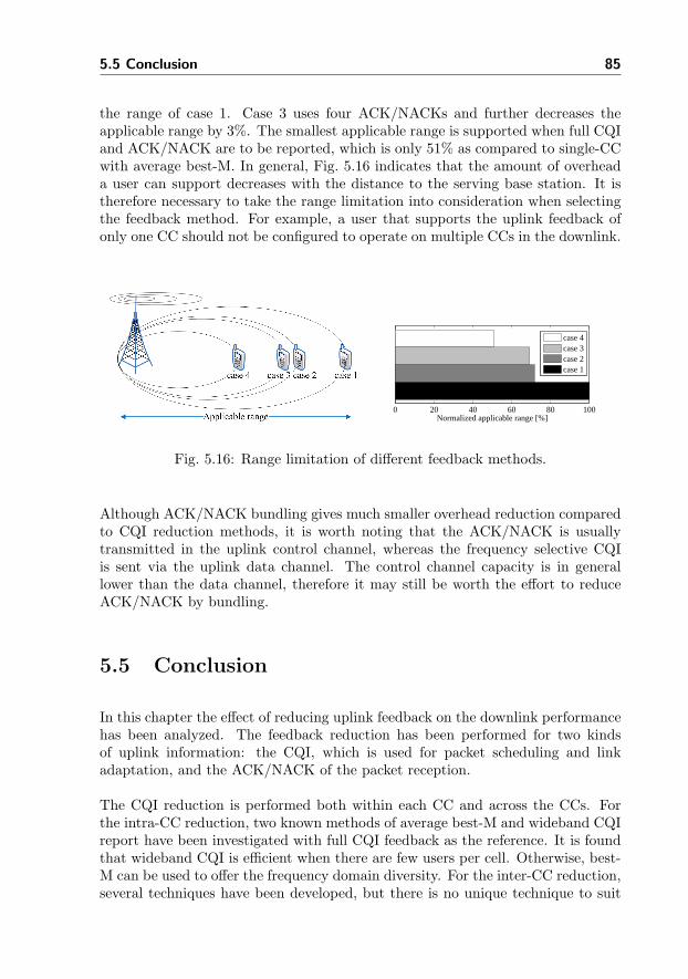
5.5 Conclusion 85
the range of case 1. Case 3 uses four ACK/NACKs and further decreases theapplicable range by 3%. The smallest applicable range is supported when full CQIand ACK/NACK are to be reported, which is only 51% as compared to single-CCwith average best-M. In general, Fig. 5.16 indicates that the amount of overheada user can support decreases with the distance to the serving base station. It istherefore necessary to take the range limitation into consideration when selectingthe feedback method. For example, a user that supports the uplink feedback ofonly one CC should not be configured to operate on multiple CCs in the downlink.
0 20 40 60 80 100Normalized applicable range [%]
case 4case 3case 2case 1
Fig. 5.16: Range limitation of different feedback methods.
Although ACK/NACK bundling gives much smaller overhead reduction comparedto CQI reduction methods, it is worth noting that the ACK/NACK is usuallytransmitted in the uplink control channel, whereas the frequency selective CQIis sent via the uplink data channel. The control channel capacity is in generallower than the data channel, therefore it may still be worth the effort to reduceACK/NACK by bundling.
5.5 Conclusion
In this chapter the effect of reducing uplink feedback on the downlink performancehas been analyzed. The feedback reduction has been performed for two kindsof uplink information: the CQI, which is used for packet scheduling and linkadaptation, and the ACK/NACK of the packet reception.
The CQI reduction is performed both within each CC and across the CCs. Forthe intra-CC reduction, two known methods of average best-M and wideband CQIreport have been investigated with full CQI feedback as the reference. It is foundthat wideband CQI is efficient when there are few users per cell. Otherwise, best-M can be used to offer the frequency domain diversity. For the inter-CC reduction,several techniques have been developed, but there is no unique technique to suit

86 Downlink Performance of Multi-CC Systems With Reduced Feedback
the transmission in all load conditions. As a result, a load adaptive CQI reductionscheme is proposed. It assigns a smaller number of CCs to the LTE-Advancedusers when the load is high, and vice versa. The proposed scheme also includesthe selection between wideband CQI and average best-M. As compared to full CQIreport, it reduces the CQI by 94% at low load, and 79∼93% at medium to highload. Throughput wise, for the realistic arrival rates that are well below the cellcapacity, it offers the same average cell throughput and less than 25% degradedcell edge user throughput. Although the reduction is performed only for the CQIin a SIMO system, the overhead of PMI and RI in a MIMO system can also bereduced by using a similar approach.
To reduce the overhead of ACK/NACK signaling, a method called ACK/NACKbundling is applied. The loss of ACK/NACK bundling decreases with the numberof users (load) per cell. In a SIMO system with 10 users per cell, having oneACK/NACK per user causes a loss of 7.5% in average cell throughput and 12%in cell edge user throughput. It is also observed that in the considered macro-cellscenario with 2 by 2 MIMO and full buffer traffic model, the number of users sup-porting rank-2 transmission is rather low, and hence bundling the ACK/NACKsof the MIMO streams (intra-CC bundling) gives no performance loss. However,for cases with a high probability of rank-2 transmissions, or higher MIMO ranks,the throughput loss due to intra-CC bundling may increase. Further investigationsare needed in order to decide the number of ACK/NACKs in the antenna domain.
The impact of overhead reduction on the uplink coverage is also analyzed based onsome simplified assumptions. The final decision of the feedback method for a usershould be made according to the cell load as well as the user uplink capability.

Chapter 6
Conclusions and Future Work
The thesis has investigated system level technologies to improve the performanceof the Long Term Evolution (LTE)-Advanced systems. LTE-Advanced should sup-port a wide bandwidth of up to 100 MHz, which is usually obtained by aggregatingseveral Component Carrier (CC)s.
Both local area and wide area scenarios have been considered in this thesis. Thereason for considering the wide area is that this is the way the traditional wirelessnetworks are deployed, and it will also be one of the most important scenariosfor the future systems. As to local area network, it has a different interferencecondition from the wide area network, due to the small cell size and the unco-ordinated placement of the Access Point (AP)s. Furthermore, it usually lacks acentral controller and hence prefers the self-organized operation. In view of theseaspects, the two scenarios have been studied separately in this thesis, and differentapproaches have been used for them. Recommendations for the LTE-Advancedsystem in local and wide area networks are provided in the following sections. Thepossible future work is listed at the end of the chapter.
6.1 Recommendations for Local Area Network
Chapter 2 investigates the performance of a local area TDD system with differentlevels of network time synchronization. It is observed that the time synchronization

88 Conclusions and Future Work
has a significant impact on the system performance. Without synchronization, theuplink transmission will be severely penalized by the interference coming from thedownlink. In order to guarantee reasonable uplink service, at least loose networktime synchronization should be achieved.
The other study carried out in local area is the performance analysis of frequencyreuse, and the development of distributed algorithms for spectrum sharing in un-planned scenarios. The results in Section 3.2 indicate that a reuse factor of 2is preferable in most cases. Afterwards, several algorithms have been developedto facilitate the spectrum sharing without the need of a central controller. Oneof the algorithms is FiDCA, it aims to achieve the optimal reuse-2 pattern byallowing each cell to jump towards the channel with low interference. Anotheralgorithm, the DS3, reduces interference by preventing cells from operating onspectrum with heavy interference. Compared to the case of reuse-1, they achievea gain of 50∼500% in cell edge user throughput, with small or no loss in averagecell throughput. The selection between these algorithms in a specific local areanetwork can be done depending on the variation range of the cell density and theprocessing capability of the AP.
Achieving network time synchronization is also needed in the wide area network,which has already been extensively studied. Furthermore, the finding from thespectrum sharing study also confirms the advantage of having frequency reuse-1in the wide area.
6.2 Recommendations for Wide Area Network
The first topic investigated for the wide area network is the carrier load balancing.It is found that the multi-user diversity is maximized when the load is strictlybalanced across the CCs. Among several existing techniques, the balancing methodof Least Load (LL), which assigns the CC with the lowest load to a user, offersthe best performance. To provide fairness among users that can access differentnumber of CCs, a cross-CC PF scheduler is proposed. It increases the schedulingpriority for the users with less CCs and hence achieves much higher cell edgeuser throughput than independent scheduling. The gain is up to 90% with fullbuffer transmission and 40% with finite buffer transmission. Meanwhile, it has nodegradation in the average cell throughput, and is therefore an attractive candidatefor the layer-2 packet scheduling.
The last topic of this study is the feedback reduction, which is carried out for twokinds of uplink information: the CQI, which is used for packet scheduling andlink adaptation; and the ACK/NACK of the packet receptions. The CQI can bereduced both within each CC and across the CCs. For the intra-CC reduction,

6.3 Future Work 89
two known methods of average best-M and wideband CQI have been investigatedwith full CQI feedback as the reference. It is found that wideband CQI is efficientwhen there are few users per cell. Otherwise, best-M is recommended to offerthe frequency domain diversity. For the inter-CC reduction, a load adaptive CQIreduction scheme is proposed. It assigns less CCs to the LTE-Advanced users whenthe load is high, and vice versa. The proposed scheme also includes the selectionbetween wideband CQI and average best-M. It significantly reduces the overhead(79∼94%) while retaining reasonable downlink performance. The ACK/NACKoverhead is reduced by bundling the multiple ACK/NACKs of a user. It alsooffers the trade-off between downlink performance and uplink overhead.
The investigated topics in the wide area are in general applicable also for the localarea network, and similar behavior is expected.
6.3 Future Work
In this thesis the local and wide area networks occupy different frequency bandsand therefore their performance has been analyzed separately. However, due thespectrum scarcity, they may be deployed on the same frequency band and theinteraction between these two kinds of networks is significant. Therefore, it isnecessary to study the case when both of them exist on the same band, e.g., theheterogeneous networks.
The investigations in the multi-CC system are mostly for the case when the aggre-gated CCs have the same channel quality and the same center carrier frequency,and users are not subject to any Quality of Service (QoS) constraint. It is neces-sary to study the performance of quality guaranteed services in combination withdifferent carrier aggregation patterns, where the CCs can differ from each other inbandwidth, carrier frequency, interference level, etc.
Several techniques have been investigated in this thesis to increase the averagecell throughput and cell edge user throughput, or to trade off between these twoperformance metrics, including Generalized Proportional Fair (GPF) scheduling,hard or fractional frequency reuse, load-adaptive average best-M, velocity depen-dent CC assignment. However, there are many others that should be considered.For instance, MIMO is a very important technique to boost the system perfor-mance. Up to 8 × 8 MIMO in the downlink and 4 × 4 in the uplink have beenapproved in 3GPP for the LTE-Advanced system. How to optimize the MIMOtransmission with the existence of multiple CCs should be investigated. Whenmulti-user MIMO is used, the transmissions can only be multiplexed for usersthat are assigned on the same CC. In this case, further investigation is needed todivide the users among the available CCs. In the uplink transmission, operating

90 Conclusions and Future Work
across a wide bandwidth requires high transmit power, which may be problematicfor users far from the base station. Therefore, the power control should also bestudied with the spectrum/CC assignment.

Appendix A
Scenario DependentSimulation Assumptions
This appendix describes the simulations assumptions for each considered scenarioin this thesis, including the indoor home and office scenarios (local area) and theoutdoor Manhattan, based on the proposal in [113], and the wide area Macro-cell scenario according to [114]. The system parameters are taken from the LTEsystem, which are likely to be used for LTE-Advanced as well.
A.1 Local Area Network
A.1.1 Home Scenario
A local area home scenario with 16 homes is considered. Each home contains 4rooms, and one room has a size of 5×5 m2. There is one AP in each home. An APis a low transmit power base station, as compared to the ones used in wide areanetworks. The house owner is completely free to place the AP wherever possible,leading to randomized AP positions. It is reasonable to assume that a user isserved by its own AP, thereby receiving service from its own AP even if the signalstrength from a neighboring AP is higher. This kind of cell selection is known asthe CSG [115,116].

92 Scenario Dependent Simulation Assumptions
Fig. A.1 gives an example of a home scenario with randomized APs (denoted bythe solid circles). Users are randomly distributed within the coverage of eachcell. Neighboring cells/homes are distinguished from each other by different col-ors. While the walls inside each home are thin walls with small attenuation loss,the ones between homes are thick, and the attenuation loss is high. The highattenuation loss to some extent offers ‘isolation’ of the individual home and helpsto improve the SINR condition.
0 5 10 15 20 25 30 35 40 45m0
5
10
15
20
25
30
35
40
45m
Fig. A.1: Indoor home scenario with 16 cells.
Due to the small number of users that are served by each local area AP, the trafficchanges very fast within each cell and quite often, one cell will be in idle modeas users connected to it do not demand any data traffic. In the snapshot basedsimulation, the probability of having traffic in a cell is controlled by a pre-definedactivity factor. In the long term, this activity factor becomes equivalent to theratio of the active APs over the total number of APs, and it also indicates the celldensity. When the total number of base stations is fixed, a high activity factormeans that more cells are active, and the density is high. In Fig. A.1 and Fig. A.2,a solid circle means an active AP, whereas an empty circle indicates an idle AP.To verify the applicability of the findings with different network sizes, a smallhome scenario is also considered for the performance evaluation. It contains only4 homes in the bottom left corner of Fig. A.1, and all APs are assumed to beactive.
A.1.2 Office scenarios
In the office scenario, the location of APs can be pre-planned so that each willcover a certain area. Fig. A.2 shows an office scenario with 16 cells. The APs

A.1 Local Area Network 93
are placed at the center of each cell, and users are randomly distributed withinthe whole area. Unlike the home scenario, which restricts a user to be served bythe AP physically located within the same cell, the users in an office scenario areable to connect to the AP with the highest channel gain (path loss and shadowingfading). This is often referred to as the OSG mode [117]. The office scenarioconsidered in this study is constituted of 16 equal-size cells, where each cell has10 rooms, separated into two rows by a corridor of 5 m width. The size of eachroom is 10 × 10 m2. The office scenario is constructed with only thin walls sothe cell isolation is worse than the home scenario. However, the coordinated APplacement and the OSG access mode prevents a user from being connected to anAP with poor channel quality while interference is high, hence better cell edgeSINR is achieved than in the home scenario. Similar as with the home scenario,a small office scenario with only 4 cells is also considered for the performanceevaluation.
0 20 40 60 80 100 120 140 160 180 200m0
20
40
60
80
100m
Fig. A.2: Indoor office scenario with 16 cells.
A.1.3 Manhattan Scenario
The Manhattan scenario is used to verify the advantage of frequency reuse-1 inwide area networks. Following [18, 113], the locations of the base stations arecoordinated such that Line of Sight (LOS) connection between neighboring basestations is avoided. Similar as in the office scenario, users are connected to thebase station with the highest path gain, i.e., the Open Subscriber Group (OSG)mode. This scenario is shown in Fig. A.3. Each block means one building of size110× 110 m2; the road has a width of 15 m.

94 Scenario Dependent Simulation Assumptions
0 200 400 600 800 1000m0
200
400
600
800
1000m
Fig. A.3: Manhattan scenario with 36 cells and coordinated base station locations.
A.1.4 General Assumptions of LTE-Advanced in Local Areaand the Manhattan Scenario
Table A.1 gives a short summary of the system assumptions for the consideredscenarios.
The snapshot based simulation is used for the performance evaluation. Within eachsnapshot, the base stations are generated according to the deployment method (atthe center of each cell or randomly located) as well as the activity factor. Arandom number of users is then generated within each active cell, which uniformlydistributes within the range of 2 to 4 in the home scenario and 5 to 10 in the officescenario. In order to get the statistically averaged performance, a few thousands ofsnapshots are simulated and the throughput is collected from all these snapshots.The Manhattan has a much larger cell coverage than the indoor networks, thereforeit has different system assumptions. To be specific, 10 outdoor users are simulatedwithin each cell, and the downlink transmit power is 30 dBm. The location &distance dependent path loss model (B1) is used. Because the outer-tier cells do nothave realistic interfering cells in the simulation, the results are collected only fromthe center 7 cells out of the 36 simulated ones. This is different from the indoorsimulations, where all simulated cells contribute to the overall performance. In theManhattan scenario, the path loss is calculated according to Table A.2 [18,113].
In Table A.2, fc is the center carrier frequency in GHz; h′BS = hBS − 1.0, h′
MS =

A.1 Local Area Network 95
Table A.1: Parameters and assumptions for system level evaluation of local areanetworks [18,113].
Parameter Setting/descriptionSpectrum allocation 100 MHz at 3.5 GHzDuplexing scheme TDDUsers per cell Home: 2∼4 users; Office: 5∼10 users; Manhat-
tan: 10 usersTransmit power AP: 24 dBm in home and office scenarios, 30 dBm
in Manhattan scenario; user: -30∼24 dBmAntenna system “Omni-directional”. AP: 3 dBi; user: 0 dBiReceiver noise figure AP: 7∼9 dB; user: 9 dBRoom size Home: 5× 5 m2; Office: 10× 10 m2
Corridor width 5 m
Indoor wall attenuation loss
{Inside home: 5 dB; between homes: 10 dBOffice: 5 dB
Indoor path loss
LOS: 18.7log10d+ 46.8 + 20log10(fc/5.0)NLOS: 20log10d+ 46.4 + nwLw + 20log10(fc/5.0)whered = direct-line distance [m]fc = carrier frequency [GHz]nw = number of walls between transmitter and receiverLw = wall attenuation [dB]
Shadow fading Uncorrelated, log-normal with 3 dB std.Minimum Coupling Loss 45 dBTraffic model Full buffer
Table A.2: Location & distance dependent path loss model for the outdoor Man-hattan scenario [18,113].
Scena-rio
Path loss [dB] Shadowfading
Applicablerange
LOSPL = 22.7log10(d1) + 41.0 + 20log10(fc/5) 3 dB std.
d1 < dBP
PL = 40.0log10(d1) + 9.45− 17.3log10(h′BS)
− 17.3log10(h′ms) + 2.7log10(fc/5.0)
d1 ≥ dBP
NLOS
PL = min{PL(d1, d2), PL(d2, d1)}wherePL(dk, dl) = PLLOS(dk) + 20− 12.5nj
+ 10nj log10(dl) + 3log10(fc/5.0)andnj = max{2.8− 0.0024dk, 1.84}k, l ∈ {1, 2}PLLOS is the pathloss of the LOS scenario.
4 dB std. d1 < 5km

96 Scenario Dependent Simulation Assumptions
hMS −1.0, where hBS = 10 m, hMS = 1.5 m are the actual antenna heights of thebase station and the user equipment; the effective environment height in urbanenvironments is assumed to be 1.0 m. dBP = 4h′
BSh′MSfc[Hz]/c, with c = 3.0×10⁸
m/s being the propagation velocity in free space.
The Non-Line of Sight (NLOS) path loss model for the outdoor Manhattan scenariois dependent on two distances, d1 and d2. These distances are defined with respectto a rectangular street grid, as illustrated in Fig. A.4. d1 is the distance from thebase station to the center of the perpendicular street, and d2 is the distance of theuser along the perpendicular street, measured from the center of the horizontalstreet where the base station is installed [18,113].
Fig. A.4: Geometry for the location & distance dependent path loss model.
A.1.5 The Physical Layer Modeling
The performance with different synchronization levels is investigated by systemlevel simulations, using a snapshot based method. One radio frame with 10 msduration is simulated for each snapshot, and the effect of the uplink-downlinkmutual interference due to imperfect network time synchronization can be seenfrom the different interference levels for the individual subframes. Within eachsnapshot, the cell layout is generated according to the scenario. For the officescenario, one AP is placed at the center of each cell, but for the home scenario,APs are randomly placed. Users are uniformly distributed inside each cell. TheError Vector Magnitude (EVM) is used to model the hardware imperfection [22],which is assumed to have a value of 3%. The use of EVM puts a maximumlimitation on the received SINR, which is:
SINRmax = −20log100.03 = 30.5dB (A.1)

A.1 Local Area Network 97
The received SINR then becomes [118]:
SINR = 1/ (1/SINRideal + 1/SINRmax) (A.2)
In (A.2), the ideal SINR is calculated from the signal power, the interference powerand the noise level. The LTE link-level capacity curve is used to map the SINRto spectral efficiency and finally the throughput. According to [68], the capacityin a Single Input Single Output (SISO) LTE system can be estimated by:
S = min {BWeff log2(1 + SINR/SINReff ), 5.02} (A.3)
where S is the estimated spectral efficiency in bps/Hz, which is upper limited ac-cording to the hard spectral efficiency given by 64-Quadrature Amplitude Modulation(QAM) with the coding rate 9/10 (5.4 bps/Hz) and the cyclic prefix (0.93); BWeff
adjusts for the system bandwidth efficiency and SINReff adjusts for the SINRimplementation efficiency. {BWeff , SINReff} has the value of {0.56, 2.0} in thedownlink, and {0.52, 2.34} in the uplink. Although (A.3) treats the interference asGaussian, it has been shown in [68] to provide an accurate throughput estimationin a multi-cell system with non-Gaussian interference.
According to the 3GPP standard [22], the local area AP transmits at a constantpower of 24 dBm in the downlink. Note that for the sake of simplicity, the samepower level is used for both home and office scenario, despite the fact that alower transmit power level of 20 dBm is specified for the home scenario. In theuplink transmission, Power control is applied to minimize the interference as wellas to prolong the user battery life [119]. The uplink power control mechanismcontains both open-loop and closed-loop operations. Specifically, the open-loopcomponent partially compensates for the pass loss [120], whereas the closed-loopcomponent offers adaptation to the channel quality variations [121–123]. Becausethe channel varies slowly in the indoor system, fast fading is not modeled andfractional path loss compensated power control is applied. The transmit power fora user is [27, 119]:
P = max {Pmin,min{Pmax, P0 + αPL}} (A.4)
where Pmin = −30 dBm, Pmax = 24 dBm, PL is the path loss value in decibelbetween a user and its serving AP. In [124], it was found that P0 = −60 dBm andα = 0.8 give a good performance in local area networks. These values are adoptedhere for the uplink power control.
To simplify the problem and focus mainly on the effect of network time synchro-nization and cell level spectrum sharing, a frequency domain channel blind FairResource (FR) scheduling is used within each cell. By using FR, each user getsan equal share of the available resources of its own cell. Full buffer traffic model isused, which assumes each user always has data to transmit or receive. As a con-sequence, all possible transmission resources would be used. Furthermore, onlyLTE-Advanced users are considered, which can access the whole spectrum.

98 Scenario Dependent Simulation Assumptions
The following metrics are used for the evaluation of the system performance:
Average cell throughput: the cell throughput averaged over all simulated cells.
Cell edge user throughput: the 5% worst user throughput from all simulatedones.
A.2 Wide Area Network
The performance of the load balancing methods, the different PS algorithms, andthe feedback reduction is evaluated in a quasi static downlink system level simula-tor that follows the LTE-Advanced specifications defined in [9], including layer-3CC selection, layer-2 PS, HARQ, link adaptation and feedback functionalities.The simulation scenario is 3GPP Macro-cell case#1 as defined in [114, 125]. Thesimulation parameters are summarized in Table A.3. The detailed assumptionsare discussed in the following.
A.2.1 Macro-cell Layout and SectorizationWithin Each Site
The macro-cell case#1 uses hexagonal site layout and an inter site distance of 500m. A three-sector antenna is mounted in each site, which sectorizes one site intothree cells. The 2-dimension antenna pattern is simulated, as [114]:
A(θ) = −min
[12
(θ
θ3dB
)2
, Am
](A.5)
where −180 ≤ θ ≤ 180 degree, θ3dB = 70 degree is the 3 dB beamwidth when theantenna gain is reduced to half the maximum value, Am = 20 dB is the maximumattenuation.
Among the 19 macro-sites, only the center-site is simulated. The surrounding sitesare used to generate time continuous interference across the full bandwidth. Theaccuracy of the center-site simulation as compared to simulating all sites (withwrap-around) is verified by the G-factor distribution presented in Fig. A.5. G-factor is the ratio of the total received wideband signal power and the interferenceplus noise power at the receiver side. It includes the effects of path loss and shadowfading, but is average over fast fading. It is equivalent to the average widebandSINR in a single antenna system.
The layout of the 19 hexagonal sites is depicted in Fig. A.6(a), and the three-sectorantenna pattern within each site is shown in Fig. A.6(b).
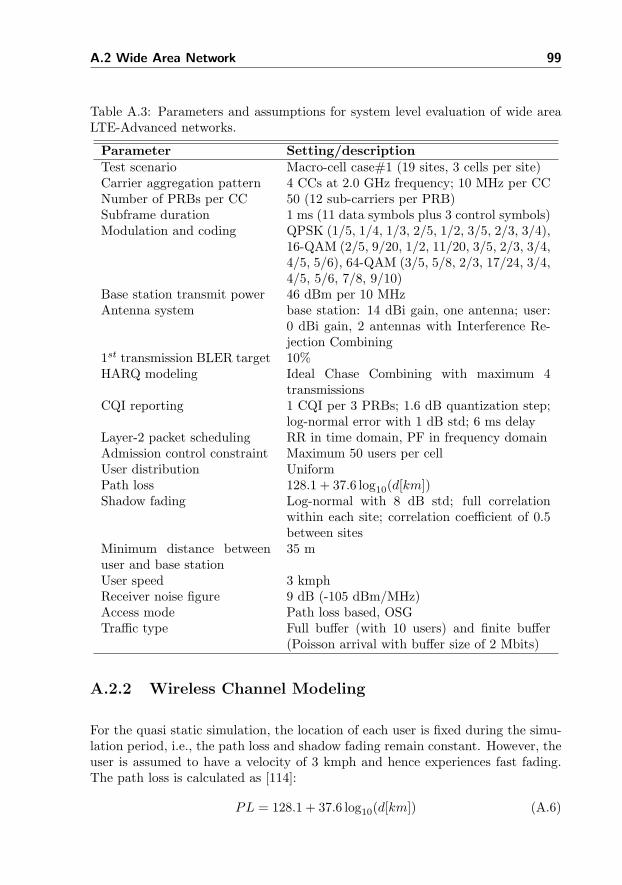
A.2 Wide Area Network 99
Table A.3: Parameters and assumptions for system level evaluation of wide areaLTE-Advanced networks.
Parameter Setting/descriptionTest scenario Macro-cell case#1 (19 sites, 3 cells per site)Carrier aggregation pattern 4 CCs at 2.0 GHz frequency; 10 MHz per CCNumber of PRBs per CC 50 (12 sub-carriers per PRB)Subframe duration 1 ms (11 data symbols plus 3 control symbols)Modulation and coding QPSK (1/5, 1/4, 1/3, 2/5, 1/2, 3/5, 2/3, 3/4),
16-QAM (2/5, 9/20, 1/2, 11/20, 3/5, 2/3, 3/4,4/5, 5/6), 64-QAM (3/5, 5/8, 2/3, 17/24, 3/4,4/5, 5/6, 7/8, 9/10)
Base station transmit power 46 dBm per 10 MHzAntenna system base station: 14 dBi gain, one antenna; user:
0 dBi gain, 2 antennas with Interference Re-jection Combining
1st transmission BLER target 10%HARQ modeling Ideal Chase Combining with maximum 4
transmissionsCQI reporting 1 CQI per 3 PRBs; 1.6 dB quantization step;
log-normal error with 1 dB std; 6 ms delayLayer-2 packet scheduling RR in time domain, PF in frequency domainAdmission control constraint Maximum 50 users per cellUser distribution UniformPath loss 128.1 + 37.6 log10(d[km])Shadow fading Log-normal with 8 dB std; full correlation
within each site; correlation coefficient of 0.5between sites
Minimum distance betweenuser and base station
35 m
User speed 3 kmphReceiver noise figure 9 dB (-105 dBm/MHz)Access mode Path loss based, OSGTraffic type Full buffer (with 10 users) and finite buffer
(Poisson arrival with buffer size of 2 Mbits)
A.2.2 Wireless Channel Modeling
For the quasi static simulation, the location of each user is fixed during the simu-lation period, i.e., the path loss and shadow fading remain constant. However, theuser is assumed to have a velocity of 3 kmph and hence experiences fast fading.The path loss is calculated as [114]:
PL = 128.1 + 37.6 log10(d[km]) (A.6)

100 Scenario Dependent Simulation Assumptions
−10 −5 0 5 10 15 200
0.2
0.4
0.6
0.8
1
Cum
mul
ativ
e di
strib
utio
n
G−factor [dB]
Center−site, no wrap aroundAll sites, with wrap around
Fig. A.5: G-factor distribution for the center-site and all-site simulation modes.
1
2
3
4
5
6
7
8
9
10
11
12
13
14
15
16
17
18
19
Distance [m]
Dis
tanc
e [m
]
G−factor [dB]
−1000 −500 0 500 1000
−1000
−500
0
500
1000
−4
−2
0
2
4
6
8
10
12
14
16
(a) 19-site macro-cell layout
−150 −100 −50 0 50 100 150−20
−10
0
Angle from the main lobe direction [degree]
Ant
enna
gai
n
0
−5
−10
−15
−20 0
30
90
150
180
270
Cell 0Cell 1
Cell 2
(b) 3-sector antenna pattern
Fig. A.6: The 19-site macro-cell layout and 3-sector antenna pattern.
All the users are modeled as indoor users, therefore an additional outdoor-to-indoor penetration loss of 20 dB is added on top of the path loss calculated using(A.6).
The shadow fading is assumed to follow a log-normal distribution with 8 dB stan-dard deviation. While fully correlated shadow fading is considered within eachsite, the shadow fading between sites is spatially correlated, with a correlation

A.2 Wide Area Network 101
coefficient of 0.5. The correlated shadow fading between user k and site i is:
Sk,i =√ρSk +
√1− ρσni (A.7)
In (A.7), ρ = 0.5 is the site correlation; σ = 8 dB is the shadow fading standarddeviation; Sk = σnk is the near-field shadow fading for user k; nk and ni arerandom variables that follow the normal distribution.
The multi-path channel is modeled using the tapped-delay model. Assuming afinite number of P distinct paths, the channel impulse response can be writtenas [12]:
h(τ) =P∑i=1
aiδ(τi) (A.8)
In (A.8), each tap is the superposition of a large number of scattered waves withapproximately the same delay of τi. ai is time varying due to the multi-pathphenomenon and the power for each tap is
∣∣a2i ∣∣. The amplitude of ai is usuallyassumed to be Rayleigh distributed and with Doppler spectrum [126]:
S(f) ∝ 1/(1− (f/fD)2)0.5 (A.9)
where fD = v/λ = vfc/c is the maximum Doppler shift, v is the mobile speed inm/s, c = 3.0× 10⁸ m/s is the speed of light, fc is the carrier frequency in Hz. Inthe 2 GHz band with user speed of 3 kmph, the maximum Doppler shift is 5.6 Hz.
In this thesis, the Typical Urban model with 20 paths (TU-20) [126] is used. Thepower delay profile for the TU-20 model is given in Table A.4.
A.2.3 Link Adaptation
The link to system mapping is based on the Exponential Effective SIR Mapping(EESM) model [127]. It calculates an effective SINR based on the individual SINRvalue within each PRB.
SINR = −β ln
(1
Nu
Nu∑k=1
e−SINRk
β
)(A.10)
In (A.10), β is a parameter optimized from link-level simulation results for eachModulation and Coding Scheme (MCS). The value of β also indicates the sensitiv-ity of turbo decoder with respect to channel variation. In general, a high level ofMCS is more sensitive to the channel variation than a low MCS and hence requiresa higher value of β. Nu is the number of sub-carriers within one PRB. The SINRvalue in (A.10) is also subject to EVM, which is assumed to be 8%, correspondingto a maximum SINR of 22 dB.
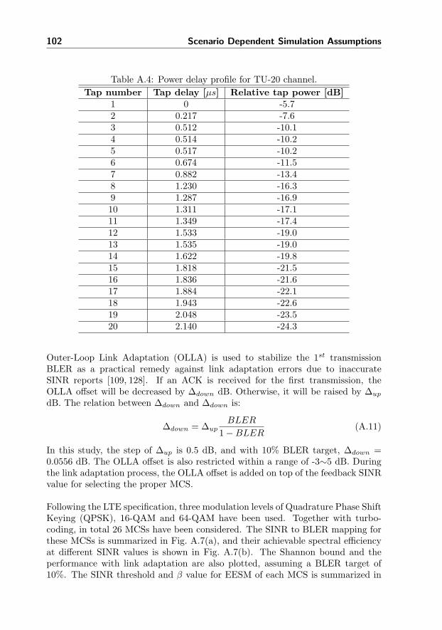
102 Scenario Dependent Simulation Assumptions
Table A.4: Power delay profile for TU-20 channel.
Tap number Tap delay [µs] Relative tap power [dB]1 0 -5.72 0.217 -7.63 0.512 -10.14 0.514 -10.25 0.517 -10.26 0.674 -11.57 0.882 -13.48 1.230 -16.39 1.287 -16.910 1.311 -17.111 1.349 -17.412 1.533 -19.013 1.535 -19.014 1.622 -19.815 1.818 -21.516 1.836 -21.617 1.884 -22.118 1.943 -22.619 2.048 -23.520 2.140 -24.3
Outer-Loop Link Adaptation (OLLA) is used to stabilize the 1st transmissionBLER as a practical remedy against link adaptation errors due to inaccurateSINR reports [109, 128]. If an ACK is received for the first transmission, theOLLA offset will be decreased by ∆down dB. Otherwise, it will be raised by ∆up
dB. The relation between ∆down and ∆down is:
∆down = ∆upBLER
1−BLER(A.11)
In this study, the step of ∆up is 0.5 dB, and with 10% BLER target, ∆down =0.0556 dB. The OLLA offset is also restricted within a range of -3∼5 dB. Duringthe link adaptation process, the OLLA offset is added on top of the feedback SINRvalue for selecting the proper MCS.
Following the LTE specification, three modulation levels of Quadrature Phase ShiftKeying (QPSK), 16-QAM and 64-QAM have been used. Together with turbo-coding, in total 26 MCSs have been considered. The SINR to BLER mapping forthese MCSs is summarized in Fig. A.7(a), and their achievable spectral efficiencyat different SINR values is shown in Fig. A.7(b). The Shannon bound and theperformance with link adaptation are also plotted, assuming a BLER target of10%. The SINR threshold and β value for EESM of each MCS is summarized in

A.2 Wide Area Network 103
Table A.5, which is used in the system level simulation.
The specific curves are generated by using Turbo receiver in TU-20 channel, wheneach user is statically scheduled with 26 PRBs (312 sub-carriers), and coding isperformed within these PRBs. According to link level simulation, it is enough toachieve maximum interleaving gain by coding across these PRBs. For cases whena user is scheduled with less number of PRBs, this physical layer mapping is abit optimistic. The accuracy in general is acceptable because the packet schedulerusually does not schedule more than 6 or 7 users in a 10 MHz bandwidth withineach TTI.
−5 0 5 10 15 2010
−3
10−2
10−1
100
Effective SINR [dB]
BLE
R
4QAM 16QAM 64QAM
(a) SINR versus BLER
0 5 10 15 200
1
2
3
4
5
6
7
Effective SINR [dB]
Spec
tral
eff
icie
ncy
[bps
/Hz]
Shannon boundLTE link adaptation
4QAM
16QAM
64QAM
(b) SINR versus spectral efficiency
Fig. A.7: Mapping from SINR to BLER and spectral efficiency.
A.2.4 Hybrid Automatic Repeat Request Management
LTE(-Advanced) makes use of HARQ to ensure success packet reception at thereceiver side. Re-transmission will take place when the previous transmissionfails. Asynchronous and adaptive HARQ is supported in LTE(-Advanced), whichmeans the re-transmission can be scheduled at any time on any PRBs. However,the same MCS should be used, such that the re-transmission can be combinedwith the previous transmission(s). In this study, the Chase Combining is used,and the SINR after Chase Combining is modeled as:
SINRn = ϵn−1n∑
k=1
SINRk (A.12)
In (A.12), SINRk is the received SINR for the kth (re-)transmission; SINRn
is the combined SINR after n transmissions, and ϵ quantizes the combining effi-

104 Scenario Dependent Simulation Assumptions
Table A.5: Link to system level mapping table.
Modulation Coding Spectral Effi-ciency [bps/Hz]
10% BLERThreshold [dB]
EESM-β
QPSK
1/5 0.4 -2.7 1.341/4 0.5 -1.3 1.571/3 0.67 -0.8 1.442/5 0.8 -0.2 1.521/2 1.0 1.3 1.533/5 1.2 2.7 1.582/3 1.33 3.4 1.583/4 1.5 4.6 1.69
16-QAM
2/5 1.6 5.3 4.339/20 1.8 6.2 4.751/2 2.0 6.8 5.2511/20 2.2 7.8 6.083/5 2.4 8.7 6.642/3 2.67 9.3 6.693/4 3.0 10.7 7.454/5 3.2 11.2 7.405/6 3.33 12.2 8.10
64-QAM
3/5 3.6 13.6 21.255/8 3.75 14.0 22.622/3 4.0 14.5 22.9117/24 4.25 15.4 25.803/4 4.5 16.3 28.744/5 4.8 16.8 29.295/6 5.0 17.8 31.077/8 5.25 18.6 33.159/10 5.4 19.2 33.78
ciency. Ideal Chase Combining is used, therefore, ϵ = 1. The maximum numberof transmissions is n = 4 in the study.
Fig. A.8: Interaction between link adaptation, HARQ and packet scheduling.

A.2 Wide Area Network 105
Fig. A.8 summarizes the interaction between OLLA, Inner-Loop Link Adaptation(ILLA), HARQ management and packet scheduling. As shown, the ACK/NACKinformation is used to adjust the OLLA offset, which is added on top of the CQIfeedback and used in ILLA. ACK/NACK also affects the HARQ managementprocess and in turn, the packet scheduling (by restricting the re-transmission touse the same MCS as the previous one). After assigning resources to the users,the packet scheduler will request ILLA to make the final decision on the MCS toeach user. The HARQ manager needs to update the stack information based onthe scheduling decision.
A.2.5 Interference Rejection Combining
In a wireless communication system with fading channel, using multiple antennasat the receiver side can exploit the spatial diversity to improve the signal quality.When the noise at the different receiving antenna branches is uncorrelated, thebest combining method is Maximal Ratio Combining (MRC), which requires theknowledge of the channel gain and the noise power per branch. However, thecellular system is usually interference limited, and the interferences at the receivingantenna branches are not fully uncorrelated. In this situation it is beneficial touse an Interference Rejection Combining (IRC) receiver to reject the dominatinginterference [129].
With one transmitting antenna and L receiving antennas, the received signal is:
r = hx+ n (A.13)
For a system with L receiving antennas and I interferers, hl,i is the complexchannel gain between the lth receiving antenna and the ith interferer. The receivedinterference-plus-noise at the lth antenna branch is:
nl = vl +I∑
i=1
Pihl,i (A.14)
where vl is the thermal noise component with variance σ2v , which is equal for all
antennas; Pi is the power of the ith interference.
The combining process in the receiver can be represented by:
y = wT r = wThx+ wTn (A.15)
In (A.15), wT is a weighting vector. Different wT corresponds to different com-bining technique. After combining, the SINR can be expressed as [130]:
SINR =E[wThhHw∗|x|2]E[wTnnHw∗]
=wThhHw∗Ps
wTRw∗ (A.16)

106 Scenario Dependent Simulation Assumptions
where Ps is the received signal power andR = E[nnH ] is the noise-plus-interferencecovariance matrix. In the case with two receiving antennas, R has the form of [130]:
R =
[ρ21 ρ1,2ρ∗1,2 ρ22
](A.17)
where ρ2l = σ2v +
I∑i=1
Pi|hl,i|2 is the received interference-plus-noise power, and
ρ1,2 =I∑
i=1
Pih1,ih∗2,i.
For the IRC receiver, a weighting vector of wT = hHR−1 is used. By insertingthis into (A.16), the output SINR of an IRC receiver is [130]:
SINRIRC = hHR−1hPs (A.18)
A.2.6 Traffic Model
Both full buffer and finite buffer traffic models are considered in the simulation,according to the guideline in [131]. The full buffer traffic model is characterized bythe fact that each user always has data to transmit or receive, and the transmissionnever finishes during a simulation run. The simulation process with the full buffertraffic is conducted as a series of simulation runs (5 seconds in each run) with aconstant number of users per cell. Different cell load can be achieved by varyingthe number of users per cell. Many simulation runs are needed to cover the userlocations within each cell. Although not very realistic in many cases, the full buffertraffic is extensively used because of the simplicity.
The finite buffer traffic model is characterized by the fact that the users havea finite amount of data to transmit or receive. Once the data transmission isfinished, the user is removed from the system. For the finite buffer model withdynamic birth-death, only one long simulation run (with duration of hundredsof seconds) is launched. This is valid because users are created and terminateddynamically during the simulation. In this study the arrival of the users is modeledas Poisson arrival, and the data associated with different users are assumed to beof the same size. By changing the Poisson arrival rate, different load conditionscan be obtained.

Appendix B
Capacity of MIMO Systemsand the Multi-user Gain
B.1 Introduction
The capacity of a wireless system can be improved in several ways, e.g., adjustthe transmission rates according to the channel quality using link adaptation [25];use MIMO multiplexing to send multiple data streams or obtain MIMO diversitygain [132,133]. In a multi-user system, the system capacity can be further improvedby exploiting the multi-user diversity using channel aware packet scheduling [24,104]. These techniques have been extensively used in many existing systems, e.g.,WiMAX [134], the 3GPP LTE [10]. They will also be applied in the forthcomingIMT-Advanced systems [46]. It is therefore worthwhile to analyze the performancecombining all these techniques.
There have been several attempts to present analytical expressions for the systemperformance in this case. Starting with references [135–139], they considered one ora combination of two of the above mentioned techniques. Reference [140] addressedall of them, but for spatial multiplexing MIMO systems only. In a real system thecapacity is limited by the highest supported modulation and coding scheme, a factthat is usually not considered in analytical derivations such as the ones mentionedabove, but have been included in simulation based analyses, e.g., in [97,141–144].Simplified approximations for a fixed number of users per cell were presented in [68]for an LTE system under various MIMO configurations and scheduling methods,

108 Capacity of MIMO Systems and the Multi-user Gain
based on simulations.
In this appendix, the exact closed form expression of the MIMO capacity in termsof average spectral efficiency is derived. Similar to [135–140], the derivation iscarried out under the assumption of uncorrelated Rayleigh fading channels and thesame average channel quality for the multiple users. Both channel blind RR andchannel aware PF [104] schedulers are investigated in the capacity analysis. Thefollowing antenna configurations are considered: the first one has one transmit andmultiple receive antennas, with MRC at the receiver. This is the same assumptionas in [136,137], however the analysis in [137] was carried out with only 3 receivingantennas, and did not address the problem in combination with channel awarepacket scheduling. The second case assumes the same number, M , of transmitand receive antennas and Zero Forcing (ZF) precoding as in e.g. [137, 140]. ZFprecoding with multi-stream transmission and link adaptation for each data streamoffers an M -fold improvement of the peak data rate as compared to single streamtransmission. When multiple users exist in a cell, the M data streams may notnecessarily come from a single user, but several users can be scheduled at a time,and each user can be allocated on multiple antennas [140]. When the channelquality is poor, multiplexing multiple data streams cannot bring any performancegain. In this situation, it is preferable to transmit with less number of data streamsto obtain diversity gain and array gain, i.e., MIMO diversity. This is known asrank adaptation, where ‘rank’ is the number of transmitted data streams. In thisappendix, the capacity expressions for the 2× 2 MIMO with rank adaptation arealso derived.
From the obtained results, it is noticed that the multi-user gain can be well ap-proximated by a logarithm function of the number of users. For the purpose ofmodeling, a summary of the approximated gain in various scenarios is given at theend of the appendix.
The rest of this appendix is organized as follows: Section B.2 describes the sys-tem model, including link adaptation, the physical link, and packet scheduling.Section B.3 provides the theoretical analysis and derives the exact closed formcapacity expressions. In Section B.4, the performance for selected cases is shown.The multi-user gain in an LTE system in both Micro- and Macro-cell scenarios ispresented in Section B.5. Finally, Section B.6 concludes the appendix.
B.2 System Model
This appendix focuses on the downlink transmission where multiple users areserved by the same base station with a constant transmit power. Fig. B.1 gives anexample of such a system. As indicated in the figure, each user first has to esti-

B.2 System Model 109
Fig. B.1: Downlink transmission in a multi-user system with uplink feedback.
mate the Channel State Information (CSI) including the SINR and the fast fadingchannel (only when channel aware precoding is used), then reports to the basestation in the uplink feedback channel. The feedback is assumed to be perfect.Based on the feedback information, the base station will format the source bits inthe proper way using link adaptation and precoding, and schedule a user with theproper resources. These techniques are described in detail in the following.
B.2.1 Link Adaptation
Link adaptation requires the selection of a proper modulation and coding schemeaccording to the channel quality which is usually indicated by the SINR value.In practical systems, due to the discrete rate levels and system imperfections, theachievable transmission rate is below the Shannon capacity and upper boundedby the highest modulation and coding scheme. It has been shown that the effectof system imperfections can be well approximated by a constant shift in the SINRvalues in the decibel scale, or by a weighting factor in the linear domain. Similarto [68,137,140], an effective SINR scaling factor is introduced to approximate theperformance of practical link adaptation. Additionally, the maximum achievablespectral efficiency Cmax is also considered. With these constraints, the mappingfrom SINR to spectral efficiency is:
S = min{log2(1 + αγ), Cmax} (B.1)
where S is the achievable spectral efficiency in bps/Hz, γ is the SINR value, andα is the effective SINR scaling factor which lies between 0 and 1. According toFig. A.7(b), the LTE link-level capacity is about 3 dB below the Shannon limit,i.e., α = 0.5. In the following analysis, α is made as an input parameter in thecapacity expressions so that the results can be generalized to systems with differentlink-level capacity.

110 Capacity of MIMO Systems and the Multi-user Gain
B.2.2 The Physical Layer Transmission
In case a large number of scatters exist, and there is no LOS link between thetransmitter and the receiver, the narrowband wireless channel is usually modeledas Rayleigh fading. As a consequence, the received SINR on each radio link isexponentially distributed with mean value of γ. γ is decided by the transmit signalstrength, the large scale channel gain resulting from path loss and shadowing, theinter-cell interference and the thermal noise level.
In a SIMO system with a single transmit antenna and M receive antennas, anMRC receiver combines the received signals, and the output SINR is ideally thesummation of the received SINRs. It follows a central chi-square distribution with2M degrees of freedom, with Probability Distribution Function (PDF) [136,145]:
pγ(x) =1
γM (M − 1)!xM−1e−x/γ (B.2)
and the CDF is:
Fγ(x) = 1− e−x/γM−1∑m=0
(x/γ)m/m! (B.3)
If a system has M transmit and receive antennas, ZF precoding can be used tosend up to M parallel data streams to a user. According to [137], the SINRper data stream still follows an exponential distribution. However, because thetransmit power is equally shared among M transmit antennas, the mean value forthe SINR per data stream is down scaled to γ/M . The PDF of the exponentiallydistributed SINR for each data stream is therefore [145]:
pγ(x) =M
γe−xM/γ (B.4)
Correspondingly, the CDF is:
Fγ(x) = 1− e−xM/γ (B.5)
When M = 1, the expressions degenerate to the SINR distribution of a SISOsystem.
In a 2 × 2 MIMO system with rank adaptation, there are two possible ranks.Rank-2 is achieved by ZF precoding, and the SINR distribution is characterizedby (B.4) and (B.5). If a user does not support rank-2 transmission, e.g., becauseof the poor channel quality, rank-1 transmission can be used to improve the SINRby exploiting the array gain and diversity gain. The analysis is carried out withthe Alamouti based Space-Time Block Code (STBC), which is widely used forthe open loop rank-1 transmission. According to [146], the received SINR for a2× 2 MIMO system with STBC is: γ = γ
2
∑i,j=1,2
gi,j , where gi,j is the fast fading

B.2 System Model 111
channel gain between the ith transmit antenna and the jth receive antenna. Thisis equivalent to the received SINR for a 1× 4 MRC system, except for a 3 dB lossin the average signal quality, due to the total power constraint. Therefore, thecapacity of the rank-1 transmission in a 2 × 2 MIMO system with average SINRof γ is the same as in a 1× 4 MRC system with SINR of γ/2.
B.2.3 Packet Scheduling
In a multi-user system, the transmission resource is shared among the existingusers. Let Ik be the scheduling indicator, in a system with K users:
Ik =
{1, user k is scheduled0, user k is not scheduled
(B.6)
With an RR scheduler all users get an equal share of the resources, irrespective oftheir instantaneous channel quality (‘Pr’ stands for ’Probability’):
Pr(Ik = 1|γk = x) = Pr(Ik = 1) = 1/K (B.7)
The PF scheduler takes the instantaneous and past averaged user data rate intoconsideration. On each data stream, it schedules resources to a user that maxi-mizes the scheduling metric rj/Rj , where j is the user index. Because the usersare assumed to have the same average channel quality, they should have the sameaverage data rate Rj . Therefore, maximizing the scheduling metric is the same asmaximizing the instantaneous data rate, or the instantaneous channel gain. Theselection of the proper user k can be formulated as:
k = argmaxj
{rj/Rj} = argmaxj
{rj} = argmaxj
{g′j} (B.8)
where Rj , rj and g′j are the past averaged data rate, the instantaneous data rateand instantaneous channel gain for user j on a given data stream. The probabilityof one user being selected when the SINR equals x is:
Pr(Ik = 1|γk = x) = Pr(γj < x,∀j = k) = Fγ(x)K−1 (B.9)
Using equations (B.2) to (B.5), the average share of resources for one user with PF
is:∞∫
x=0
pγ(x)Fγ(x)K−1dx = 1/K for both SIMO and MIMO systems. Therefore,
PF is exactly fair in terms of resource allocation among the multiple users, oncondition that they have the same average channel quality.

112 Capacity of MIMO Systems and the Multi-user Gain
B.3 Derivation of the System Capacity with PacketScheduling
Using the multi-antenna system model described in Section B.2, it is possible toderive the system capacity in terms of average spectral efficiency. The capacityin a system with S data streams (S = 1 for SIMO, and S = M for MIMO withZF precoding) is dependent on the number of users in a cell, the instantaneousspectral efficiency limit (B.1), the received SINR distribution (B.2) or (B.4), andthe scheduling probability (B.7) or (B.9). It can be expressed as:
C(M,K,α, γ, Cmax) =
KS
∞∫0
min{log2(1 + αx), Cmax}pγ(x)Pr(Ik = 1|γk = x)dx (B.10)
In a SIMO system, maximum one data stream is sent to each user at a time,this gives S = 1 in (B.10). With a PF scheduler, a user with high instantaneouschannel gain is more likely to be scheduled than another one with poor channelgain, as shown in (B.9). Inserting (B.2) and (B.9) into (B.10) leads to:
CSIMO,PF (M,K,α, γ, Cmax) = K
∞∫0
min{log2(1 + αx), Cmax}pγ(x)Pr(Ik = 1|γk = x)dx
=K
γM (M − 1)!
∞∫0
min{log2(1 + αx), Cmax}xM−1e−x/γ
(1 − e
−x/γM−1∑m=0
(x/γ)m
m!
)K−1
dx (B.11)
=K
γM (M − 1)!
∞∫0
min{log2(1 + αx), Cmax}xM−1e−x/γ
K−1∑k=0
(K − 1
k
)(−1)
ke−kx/γ
(M−1∑m=0
(x/γ)m
m!
)k
dx
After the expansion of the power of the summation, and some algebra, the aboveequation becomes:
CSIMO,PF (M,K,α, γ, Cmax) =K
γM (M − 1)!
K−1∑k=0
(−1)k(K − 1
k
) k∑n0=0
· · ·nM−3∑
nM−2=0
M−1∏m=0
(nm−1nm
)(1/m!)nm−1−nm
γ
M−1∑m=1
m(nm−1−nm)
F(α,
k + 1
γ,M − 1 +
M−1∑m=1
m(nm−1 − nm), Cmax
)(B.12)
with n−1 = k, and nM−1 = 0. The derivation of the function F(α, λ, n, Cmax) ispresented in the end of the appendix, and its expression is shown in (B.31). Thisfunction is also used for the expression of the other investigated multi-antennaschemes and packet schedulers. Equation (B.12) is applicable only when M ≥ 2,the expression for a SISO system can be obtained by setting M = 1 in the MIMOcapacity expression that is presented in the following.
In a MIMO system with ZF precoding, M data streams are sent in each time slot.According to the PDF distribution of (B.4) and the scheduling probability (B.9),

B.4 Numerical Results 113
the system capacity with PF scheduling is:
CMIMO,PF (M,K,α, γ, Cmax) = KM
∞∫0
min{log2(1 + αx), Cmax}pγ(x)Pr(Ik = 1|γk = x)dx
= KM2/γ
∞∫0
min{log2(1 + αx), Cmax}e−xM/γ(1 − e
−xM/γ)K−1
dx
= KM2/γ
K−1∑k=0
(−1)k(K − 1
k
) ∞∫0
min{log2(1 + αx), Cmax}e−xM(1+k)/γdx
= KM2/γ
K−1∑k=0
(−1)k(K − 1
k
)F(α,M(1 + k)/γ, 0, Cmax) (B.13)
The performance with an RR scheduler can be derived in a similar manner aswith PF. Alternatively, it can also be expressed using the derived formulas for PF.This is possible because the RR scheduler cannot exploit the multi-user diversity.Therefore, its average spectral efficiency is insensitive to the number of users in asystem, and is identical to the performance of PF in a single-user case (K = 1):
CSIMO,RR(M,α, γ, Cmax) = CSIMO,PF (M, 1, α, γ, Cmax)
=1
γM (M − 1)!F(α, 1/γ,M − 1, Cmax) (B.14)
CMIMO,RR(M,α, γ, Cmax) = CMIMO,PF (M, 1, α, γ, Cmax)
= (M2/γ)F(α,M/γ, 0, Cmax) (B.15)
In a system with 2 transmit and receive antennas, according to the discussion inSection B.2, the capacity for rank-1 transmission equals:
C2×2,rank−1(K,α, γ, Cmax) = CSIMO(4,K, α, γ/2, Cmax) (B.16)
Equation (B.16) is valid for both RR and PF schedulers, therefore the dependenceof the packet scheduler is dropped in the expression. Rank adaptation then choosesthe proper rank to maximize the system capacity.
B.4 Numerical Results
In Section B.3, the capacity expressions for various antenna configurations andpacket schedulers have been derived. With these expressions, the system perfor-mance can be obtained and the multi-user gain can be calculated from the relativecapacity of PF as compared to a single user system (or with RR). For the numer-ical evaluation, the SINR scaling factor of α = 0.5 is used, which corresponds to 3dB loss from the Shannon boundary. With 64-QAM and coding rate of 9/10 as thehighest modulation and coding scheme, Cmax = 5.4 bps/Hz. The output of thederived expressions are compared with Monte Carlo simulations for verification.

114 Capacity of MIMO Systems and the Multi-user Gain
B.4.1 Verification of the Capacity Expressions
First, both estimated and simulated capacity for PF with different antenna config-urations is obtained, as shown in Fig. B.2. In order to see how multi-user diversityaffects the system performance, the number of users are varied from 1 to 20, at anaverage SINR of 5 dB. RR has the same performance as single-user PF, thereforeRR is not explicitly plotted in the figure. From this figure it can be seen thatthere is an excellent agreement between the analytical predictions and the simu-lated results, confirming the validity of the derived expressions. It is also observedthat the relative performance between MIMO-ZF precoding and SIMO-MRC issensitive to the level of multi-user diversity. When the number of users is low, it isbetter to exploit the diversity gain offered by multi-antenna transmission. Whenthe number of users is high, the PF scheduler can find a good user for each datastream, therefore MIMO multiplexing is preferable.
5 10 15 201.5
2
2.5
3
3.5
4
4.5
5
Number of users in a cell
Cel
l cap
acity
with
PF
[bps
/Hz]
MIMO 4x4, estimationMIMO 4x4, simulation
SIMO 1x4, estimationSIMO 1x4, simulation
Fig. B.2: Estimated and simulated capacity with 1× 4 and 4× 4 antenna configu-rations and the PF scheduler. Performance is evaluated with different number ofusers, and an average SINR of 5 dB for each user.
Next the performance at different channel quality levels is analyzed. The numberof users in a system is assumed to be 5, and the scheduler of both RR and PFare considered. The results are summarized in Fig. B.3. Similar as Fig. B.2, it isfound that 4 × 4 MIMO with ZF precoding is not always beneficial as comparedto a 1× 4 SIMO system with an MRC receiver. In fact, at very low SINR valuesthe performance of 4×4 MIMO with ZF precoding is even worse than 1×4 MRC.The reason is that, when the SINR is low, log2(1+γ) ≈ log2(e)γ and the capacity
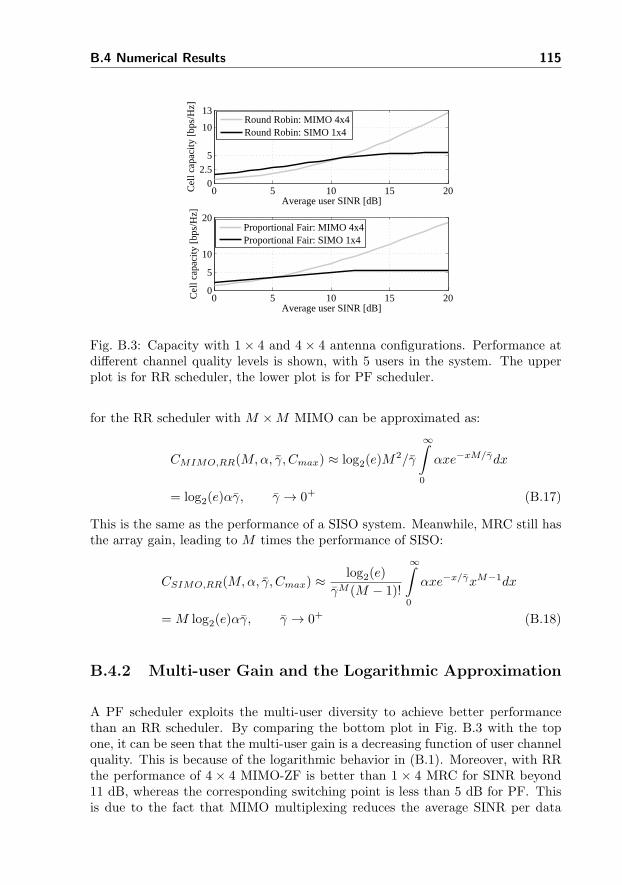
B.4 Numerical Results 115
0 5 10 15 200
2.55
10
13
Average user SINR [dB]C
ell c
apac
ity [
bps/
Hz]
Round Robin: MIMO 4x4Round Robin: SIMO 1x4
0 5 10 15 200
5
10
20
Average user SINR [dB]
Cel
l cap
acity
[bp
s/H
z]
Proportional Fair: MIMO 4x4Proportional Fair: SIMO 1x4
Fig. B.3: Capacity with 1 × 4 and 4 × 4 antenna configurations. Performance atdifferent channel quality levels is shown, with 5 users in the system. The upperplot is for RR scheduler, the lower plot is for PF scheduler.
for the RR scheduler with M ×M MIMO can be approximated as:
CMIMO,RR(M,α, γ, Cmax) ≈ log2(e)M2/γ
∞∫0
αxe−xM/γdx
= log2(e)αγ, γ → 0+ (B.17)
This is the same as the performance of a SISO system. Meanwhile, MRC still hasthe array gain, leading to M times the performance of SISO:
CSIMO,RR(M,α, γ, Cmax) ≈log2(e)
γM (M − 1)!
∞∫0
αxe−x/γxM−1dx
= M log2(e)αγ, γ → 0+ (B.18)
B.4.2 Multi-user Gain and the Logarithmic Approximation
A PF scheduler exploits the multi-user diversity to achieve better performancethan an RR scheduler. By comparing the bottom plot in Fig. B.3 with the topone, it can be seen that the multi-user gain is a decreasing function of user channelquality. This is because of the logarithmic behavior in (B.1). Moreover, with RRthe performance of 4 × 4 MIMO-ZF is better than 1 × 4 MRC for SINR beyond11 dB, whereas the corresponding switching point is less than 5 dB for PF. Thisis due to the fact that MIMO multiplexing reduces the average SINR per data

116 Capacity of MIMO Systems and the Multi-user Gain
stream as compared to single stream transmission, and hence increases the multi-user gain. On the other hand, MIMO (or SIMO) diversity reduces the variation inchannel quality and increases the average SINR; both have an effect of reducingthe multi-user gain. Therefore, a channel aware packet scheduler favors MIMOmultiplexing more than SIMO/MIMO diversity.
1 2 4 6 8 10 12 14 16 18 201
1.5
2
2.5
3
Number of users
Mul
ti−us
er g
ain
2x2: exact2x2: approx.
4x4: exact4x4: approx.
1x2: exact1x2: approx.
1x4: exact1x4: approx.
Fig. B.4: Multi-user gain with different antenna configurations, with average SINRof 5 dB.
The multi-user gain versus the number of users is plotted in Fig. B.4, for bothSIMO and MIMO systems at an average SINR of 5 dB. It is observed that whenthe capacity limit Cmax is not reached, the multi-user gain roughly follows alogarithm function of the number of users. By using curve fitting over a largevariation of average channel levels and antenna configurations, with the targetof minimizing the mean square error between the approximated and the originalvalues, the following approximation function is obtained:
GMIMO(M,K,α, γ, Cmax)
≈
1, K = 1
min
{Gmax(K), 1.1 + 0.46
(Mαγ
)log10 2
ln(K)
}, K > 1
(B.19)
Gmax(K) is the upper bound of multi-user gain, which is obtained when the SINRper data stream is so small that the mapping from SINR to spectral efficiency islinear. In this case, the average spectral efficiency with PF is
CMIMO,PF (M,K,α, γ, Cmax) ≈ log2(e)αγKK−1∑k=0
(K − 1
k
)(−1)k
(1 + k)2, γ → 0+
Under the same condition, the capacity with RR is log2(e)αγ, as shown in (B.17).

B.4 Numerical Results 117
Therefore,
Gmax(K) = KK−1∑k=0
(K − 1
k
)(−1)k
(1 + k)2
In fact, Gmax(K) is the same as the multi-user expression derived in [140], wherethe linear mapping from SINR to spectral efficiency is used. Equation (B.19)shows that the multi-user gain will increase with M , but decrease with αγ. Thisis due to the fact that the spectral efficiency varies relatively less in high SINRregion than in low SINR region.
Different from MIMO with ZF precoding, the gain with MRC decreases with thenumber of receiving antennas. For very high values of M , or αγ, the variation ininstantaneous spectral efficiency is small, and there will hardly be any multi-usergain. Similarly, with 1 × M SIMO, the multi-user gain can be approximated inthe logarithmic form:
GSIMO(M,K,α, γ, Cmax) (B.20)
≈
{1, K = 1
max{1, 1.14− 0.02(M + log10(αγ)) +
0.46M(αγ)log10 2 ln(K)
}, K > 1
The approximated multi-user gain is also plotted in Fig. B.4, and it is close tothe one obtained from simulation or the derived capacity expressions. It is worthnoting that (B.19) and (B.20) are valid when the capacity limit is not reached. Ifthe channel quality is so good that Cmax is often reached, the multi-user gain willbe significantly lower than shown here.
B.4.3 Performance of MIMO Rank Adaptation
The obtained results confirm that, when the channel quality is poor, it is better touse MIMO diversity to increase the signal strength rather than to transmit overmultiple streams (the multiplexing gain). Therefore, MIMO rank adaptation isbeneficial in the sense that it can adjust the number of transmitting data streamsaccording to the channel condition. Using the derived equations of (B.13), (B.15)and (B.16), the performance of rank-1 and rank-2 transmissions in a 2× 2 MIMOsystem can be calculated. The results in a system with 5 users are shown inFig. B.5, where rank-1 achieves a better performance than rank-2 at low SINRvalues. In the high SINR region, rank-2 transmission overcomes the performanceof rank-1. Also, PF favors the rank-2 transmission since it reduces the switchingpoint for rank adaptation from 12.5 dB (RR) to 2.5 dB.

118 Capacity of MIMO Systems and the Multi-user Gain
0 5 10 15 200
2.5
5
10
Average user SINR [dB]
Cel
l cap
acity
[bps
/Hz]
Round Robin, 2x2 MIMO: rank−1Round Robin, 2x2 MIMO: rank−2
0 5 10 15 200
2.5
5
1011
Average user SINR [dB]
Cel
l cap
acity
[bps
/Hz]
Proportional Fair, 2x2 MIMO: rank−1Proportional Fair, 2x2 MIMO: rank−2
Fig. B.5: Capacity of a 2× 2 MIMO system with different ranks. Performance atdifferent channel quality levels is shown, with 5 users in a system. The upper plotis for RR scheduler, the lower plot is for PF scheduler.
B.5 Multi-user Gain in LTE Systems
The capacity expressions derived in Section B.3 are constricted by the assumptionof having the same average channel quality for the users, so that PF is also fair inthe sense of resource sharing. The accuracy of these expressions has been verifiedby simple simulations in Section B.4. It is observed from Section B.4 that themulti-user gain follows approximately a logarithmic function with the number ofusers in a cell. The aim of this section is to verify that the logarithmic behavior ofthe multi-user gain also exists in realistic LTE systems, where users are randomlydistributed within the cell coverage area and have different average channel quali-ties. Other than the Macro-cell scenario that has been used in previous chapters,the Micro-cell scenario is also considered. Sectorization as in Macro-cell scenariois not used in the Micro-cell. The Micro-cell has a small coverage with inter sitedistance of 130 m and a different path loss model. As a consequence, the averagechannel quality with Micro-cell is better than with Macro-cell [147]. Details aboutthe Micro-cell scenario can be found in [114].
With realistic assumptions as listed in Table A.3, the system performance andthe multi-user gain are impacted due to the impairments. The multi-user gainin a Macro-cell in both average cell throughput and cell edge user throughput ispresented in Fig. B.6. The performance is shown for bandwidths from 5 to 20MHz, and clearly shows the independency of the multi-user gain from the systembandwidth (given that the bandwidth is wide enough). Despite the various systemimpairments, it is noticed that the multi-user gain follows a logarithmic function

B.5 Multi-user Gain in LTE Systems 119
5 10 15 201
1.1
1.2
1.3
1.4
1.5
1.6
Number of users
Mul
ti−us
er g
ain
in m
acro
−ce
ll
Average cell: 5 MHzAverage cell: 10 MHzAverage cell: 15 MHzAverage cell: 20 MHzAverage cell: approx.
Cell edge: 5 MHzCell edge: 10 MHzCell edge: 15 MHzCell edge: 20 MHzCell edge: approx.
Fig. B.6: Multi-user gain in Macro-cell LTE with 1× 2 SIMO. Simulation resultsfor different bandwidth settings are approximated using logarithm functions.
of the number of users per cell. Furthermore, the gain saturates when the numberof users is relatively high. This is mainly due to the granularity when performingscheduling and link adaptation. The curve-fitted expressions for the multi-usergain in the Macro-cell scenario are presented in (B.21) and (B.22) for both averagecell and cell edge user throughput, respectively.
Gmacro,averge(K) =Cmacro,average(K)
Cmacro,average(1)=
1, K = 10.11ln(K) + 1.10, 1 < K ≤ 131.38, K > 13
(B.21)
Gmacro,edge(K) =KCmacro,edge(K)
Cmacro,edge(1)=
{1, K = 10.15ln(K) + 1.05, K > 1
(B.22)
Note that the multi-user gain in cell edge user throughput is scaled by the resourcesharing per user. The above two equations are valid for a uniform distribution ofusers over the cell area, with K being the number of users per cell.
The corresponding performance in Micro-cell is presented in Fig. B.7, but for 10MHz bandwidth configuration only. Similar as in the Macro-cell scenario, themulti-user gain can also be approximated using the logarithmic function:
Gmicro,average(K) =Cmicro,average(K)
Cmicro,average(1)=
1, K = 10.05ln(K) + 1.06, 1 < K ≤ 111.18, K > 11
(B.23)
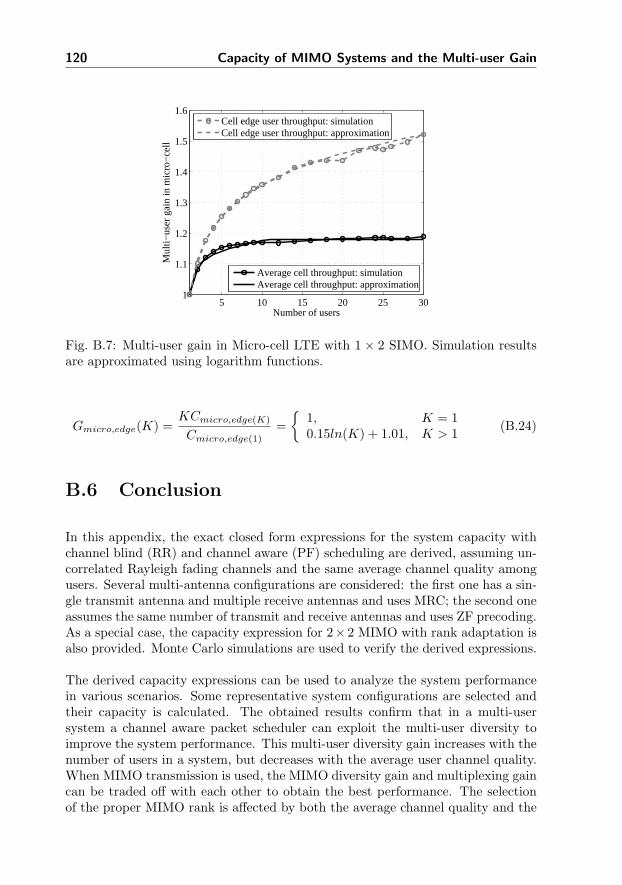
120 Capacity of MIMO Systems and the Multi-user Gain
5 10 15 20 25 301
1.1
1.2
1.3
1.4
1.5
1.6
Number of users
Mul
ti−us
er g
ain
in m
icro
−ce
ll
Average cell throughput: simulationAverage cell throughput: approximation
Cell edge user throughput: simulationCell edge user throughput: approximation
Fig. B.7: Multi-user gain in Micro-cell LTE with 1× 2 SIMO. Simulation resultsare approximated using logarithm functions.
Gmicro,edge(K) =KCmicro,edge(K)
Cmicro,edge(1)=
{1, K = 10.15ln(K) + 1.01, K > 1
(B.24)
B.6 Conclusion
In this appendix, the exact closed form expressions for the system capacity withchannel blind (RR) and channel aware (PF) scheduling are derived, assuming un-correlated Rayleigh fading channels and the same average channel quality amongusers. Several multi-antenna configurations are considered: the first one has a sin-gle transmit antenna and multiple receive antennas and uses MRC; the second oneassumes the same number of transmit and receive antennas and uses ZF precoding.As a special case, the capacity expression for 2× 2 MIMO with rank adaptation isalso provided. Monte Carlo simulations are used to verify the derived expressions.
The derived capacity expressions can be used to analyze the system performancein various scenarios. Some representative system configurations are selected andtheir capacity is calculated. The obtained results confirm that in a multi-usersystem a channel aware packet scheduler can exploit the multi-user diversity toimprove the system performance. This multi-user diversity gain increases with thenumber of users in a system, but decreases with the average user channel quality.When MIMO transmission is used, the MIMO diversity gain and multiplexing gaincan be traded off with each other to obtain the best performance. The selectionof the proper MIMO rank is affected by both the average channel quality and the

B.6 Conclusion 121
level of multi-user diversity in the system.
Based on the obtained results, it is found that the multi-user gain can be approxi-mated by a logarithmic function in the number of users. This finding is also validin LTE systems with realistic assumptions, and the approximation expressions areobtained for a couple of cases of interest.
Derivation of the Function F(·) for the CapacityExpressions
This section provides the derivation of the integration∞∫0
min{log2(1+αx), Cmax}e−λxxndx,
which is used in the expressions of the system capacity in Section B.3. Startingfirst with a variable substitution y = 1 + αx:
∞∫0
min{log2(1 + αx), Cmax}e−λxxndx
= log2 e
∞∫0
min{ln(1 + αx), Cmaxln(2)}e−λxxndx (B.25)
=log2 e
α
∞∫1
min{ln(y), Cmaxln(2)}e−λ(y−1)/α(y − 1)nα−ndy (B.26)
By using the binomial expansion and interchanging between the integration andfinite sum, (B.25) becomes:
∞∫0
min{log2(1 + αx), Cmax}e−λxxndx
=eλ/α log2 e
αn+1
n∑t=0
(n
t
)(−1)t
∞∫1
min{ln(y), Cmaxln(2)}e−λy/αyn−tdy
=eλ/α log2 e
αn+1
n∑t=0
(n
t
)(−1)t
2Cmax∫1
ln(y)e−λy/αyn−tdy
+Cmaxe
λ/α
αn+1
n∑t=0
(n
t
)(−1)t
∞∫2Cmax
e−λy/αyn−tdy
= Ψ+Φ (B.27)

122 Capacity of MIMO Systems and the Multi-user Gain
where Ψ and Φ are the first and the second component of (B.27). Let f(y) = ln(y),
and g(y) =∫e−λy/αyn−tdy = −e−λy/α
n−t∑h=0
(n−t)!h!
(αλ
)n−t−h+1yh. According to
the rule of integration by parts, i.e.,b∫a
f(y)g′(y)dy = f(y)g(y)|ab −b∫a
f ′(y)g(y)dy,
Ψ is re-written as
Ψ = −Cmaxeλ/α−2Cmaxλ/α
λn+1
n∑t=0
(n
t
)(−1)t
n−t∑h=0
(n− t)!
h!
(λ
α
)t+h
2hCmax
+eλ/α log2 e
λn+1
n∑t=0
(n
t
)(−1)t
2Cmax∫1
e−λy/αn−t∑h=0
(n− t)!
h!
(λ
α
)t+h
yh−1dy
= Ψ1 +Ψ2 (B.28)
In (B.28), Ψ1 and Ψ2 are the first and the second component of Ψ. Interchangingintegration and finite sum for Ψ2 gives:
Ψ2 =eλ/α log2 e
λn+1
n∑t=0
(n
t
)(−1)t
n−t∑h=0
(n− t)!
h!
(λ
α
)t+h2Cmax∫1
e−λy/αyh−1dy
=eλ/α log2 e
λn+1
n∑t=0
n!
t!
(−λ
α
)t n−t∑t=0
(Γ(h, λ/α)− Γ(h, 2Cmaxλ/α)
)/h! (B.29)
where Γ(s, x) =∞∫x
ts−1e−tdt is the incomplete gamma function with s = 0, 1, 2, . . ..
Γ(0, x) =∞∫x
e−t/tdt = Ei(x) is the exponential integral function, and Γ(1, x) =
e−t. The second component in (B.27) is:
Φ =Cmaxe
λ/α
αn+1
n∑t=0
(n
t
)(−1)t
∞∫2Cmax
e−λy/αyn−tdy
=Cmaxe
λ/α
αn+1
n∑t=0
(n
t
)(−λ
α
)t
(n− t)!e−2Cmaxλ/αn−t∑h=0
(2Cmaxλ/α)h
h!
=Cmaxe
λ/α−2Cmaxλ/α
λn+1
n∑t=0
(n
t
)(−1)t
n−t∑h=0
(n− t)!
h!
(λ
α
)t+h
2hCmax(B.30)

B.6 Conclusion 123
From (B.28) and (B.30) it can be seen that Φ and Ψ1 cancel each other, therefore,the integration of (B.25) is:
∞∫0
min{log2(1 + αx), Cmax}e−λxxndx
= Φ1 +Φ2 +Ψ
=eλ/α log2 e
λn+1
n∑t=0
n!
t!
(−λ
α
)t n−t∑t=0
(Γ(h, λ/α)− Γ(h, 2Cmaxλ/α)
)/h!
= F(α, λ, n, Cmax) (B.31)
If not considering the maximum capacity limit, Γ(s,∞) = 0 and (B.31) degeneratesto:
∞∫0
log2(1 + αx)e−λxxndx
=eλ/α log2 e
λn+1
n∑t=0
n!
t!
(−λ
α
)t n−t∑t=0
(n− t)!
h!Γ(h, λ/α) = F(α, λ, n) (B.32)
In the case of M ×M MIMO and ZF precoding, n equals 0 in (B.25), which gives:
∞∫0
min{log2(1 + αx), Cmax}e−λxxndx
=eλ/α log2 e
λ
(Ei(λ/α)− Ei(2Cmaxλ/α)
)= F(α, λ, 0, Cmax) (B.33)

124 Capacity of MIMO Systems and the Multi-user Gain

Appendix C
Theoretical Analysis of theFinite Buffer Transmission
In Chapter 4, the multi-Component Carrier (CC) system performance has beenanalyzed, mainly based on simulations. Both the full buffer and finite buffer trafficmodels are used and the full buffer results are verified by theoretical estimations.This appendix provides the theoretical analysis of the finite buffer transmission.The purpose is to verify the accuracy of the finite buffer simulation results.
The developed analytical model is valid for both single-CC and multi-CC systems.For the multi-CC systems, the analysis considers the case when all users are LTE-Advanced (assigned on all CCs), or all are Rel’8, which relies on carrier loadbalancing, e.g., Least Load (LL) or Mobile Hashing (MH), to select one CC peruser.
C.1 The Birth-Death Model
The arrival, or departure, of users in a network is usually modeled as a birth-death process, as shown in Fig. C.1. The birth-death process is a special case ofa continuous time Markov process, where the states represent the current numberof active users, and the transitions are between neighboring states. The ‘birth’ isthe transition towards increasing the active number of users by 1, and a ‘death’

126 Theoretical Analysis of the Finite Buffer Transmission
is the transition towards decreasing the number of active users by 1 [148]. Thefollowing notations are used for the considered traffic model:
Sk System state with k users being servedλk Arrival rate in state k, in users per secondµk Service rate in state k; in users per second
(the average service time is µ−1k )
A Maximum number of users each cell can serve
Fig. C.1: The birth-death process in queueing modeling. λk is the arrival rategoing from state k to state k+1 (a ‘birth’); µk is the departure rate of going backto state k − 1 (a ‘death’).
The admission control in LTE(-Advanced) is assumed to limit the number of usersper cell to maximum A users. This leads to the following arrival rate:
λk =
{λ, 0 ≤ k < A0, k ≥ A
(C.1)
0 0.5 1 1.5 20
0.2
0.4
0.6
0.8
1
Service time [second]
Cum
mul
ativ
e di
stri
butio
n
Simulation with finite bufferNegative exponential approximation
Fig. C.2: Service time: simulation result and its approximation.
The service time (time required for a user to finish its transmission) is usuallyassumed to follow a negative exponential distribution in voice transmission [149].

C.2 Analysis When Each User Can Access the Whole Bandwidth 127
This assumption is roughly valid also for the data traffic, where users take differenttime to download a finite buffer due to channel quality variations. In Fig. C.2, theCumulative Distribution Function (CDF) for the service time with arrival rate of20/second/cell, and buffer size of 2 Mbits is shown. The LTE-Advanced system asdescribed in Table A.3 is used, with independent scheduling per CC. According tosimulation, the average service time is 0.36 second. The approximation is thereforeperformed using a negative exponential distribution, with CDF of F (x) = 1−e−λx,and λ = 1/0.36 = 2.8. This figure shows that in general the approximation isaccurate, with small deviations for users that have very short service time.
With the exponential assumption for the service time, the probability of the systembeing at state Sk is given by [54]:
Pk =
{P0
∏k−1i=0
λi
µi+1, 1 ≤ k ≤ A
0, k > A(C.2)
where P0 is the probability of being in state S0, and
A∑k=0
Pk = 1 (C.3)
Inserting (C.2) into (C.3), the following equation is obtained:
P0 =
(1 +
A∑k=1
k∏i=1
(λi/µi+1)
)−1
(C.4)
C.2 Analysis When Each User Can Access theWhole Bandwidth
This section provides the analytical model for the case when each user can accessthe whole bandwidth, i.e., a single-CC system, or a multi-CC system with onlyLTE-Advanced users.
C.2.1 Analytical Estimations
By using channel aware packet scheduling, the multi-user diversity can be exploitedto improve the system performance. Therefore, the service rate at state Sk (k usersserved) can be expressed by using the throughput and the buffer size, as
µk =
{CF
G(k)G(∞) , 0 ≤ k < A
0, k ≥ A(C.5)

128 Theoretical Analysis of the Finite Buffer Transmission
where C is the average cell throughput, obtained when the cell load is high enoughsuch that the multi-user gain saturates; F is the buffer size for the user packettransmission; G(·) is a logarithmic function to approximate the multi-user gain,as presented in (B.21).
Inserting (C.1) and (C.5) into (C.2), the probability of the system being in stateSk can be expressed as
Pk =
P0
k−1∏i=0
λi
µi+1= P0(λF/C)k
k∏i=1
G(∞)/G(i), 1 ≤ k ≤ A
0, k > A(C.6)
Equation (C.6) is a function of the arrival rate λ, the buffer size F , the capacitylimit C, the multi-user gain G(·) and the admission control limit A. Once theseassumptions are known, an estimation of the system being in each state can beobtained.
0 10 20 30 40 500
0.1
0.2
0.3
0.4
0.5
Number of active users per cell
Prob
abili
ty
SimulationEstimation
10 arrivals/second/cell
20 arrivals/second/cell
30 arrivals/second/cell
Fig. C.3: Probability of a cell being in different states of a Markov chain.
It has been shown in [108] that in a system with assumptions listed in Table A.3and using the finite buffer model, the capacity in a 40 MHz system is 49 Mbps,i.e., C = 49 in (C.6). With maximum 50 admitted users (A = 50), the probabilityat different arrival rates are obtained both using (C.6) and from simulation, whichis plotted in Fig. C.3. As can be seen from this figure, there is a good agreementbetween the theoretical estimation and the simulation result. As the arrival rateincreases, the system is more likely to be in a state with more active users. If thearrival rate is larger than the cell can accommodate, some users cannot get enoughresources, and they will remain in the system; in this case, the number of userswill increase over time to A, and thereafter remain at that level.
The average number of active users per cell can also be estimated using (C.6), as

C.2 Analysis When Each User Can Access the Whole Bandwidth 129
5 10 15 20 25 300
10
20
30
40
50
Number of arrivals per cell per second (buffer size: 2 Mbits)
Ave
rage
num
ber
of a
ctiv
e us
ers
per
cell
SimulationEstimation
Fig. C.4: Average number of active users at different arrival rates.
K =A∑
k=1
kPk. This is compared with simulation results in Fig. C.4, and again,
with a good match between the two.
C.2.2 Comparison between Single and Multi-CC Systems
The analysis before is valid for both the single-CC case and the multi-CC case whenonly the LTE-Advanced users exist. A comparison between these two systems isgiven in this section. For a fair comparison, the buffer size and the admissioncontrol limit is kept the same, but the arrival rate is proportional to the systembandwidth, i.e., the 4-CC system is evaluated with 4 times the arrival rates of thesingle-CC system.
According to (C.6), the probability of one CC having k users is the same forthe two systems, therefore, the user throughput should be proportional to thesystem bandwidth. It is also quite intuitive, that more spectrum should bringmore throughput. This is witnessed in Fig. C.5, where a 4-CC system achieves 4times the average cell throughput and cell edge user throughput of a single CCsystem. Therefore, it verifies that the implementation of the bandwidth extensionis correct.

130 Theoretical Analysis of the Finite Buffer Transmission
12.2
48.8
1.25xN 2.5xN 2.75xN 5.0xN 6.25xN 7.5xN2.5
10
20
30
40
50
Number of arrivals per cell per second (buffer size: 2 Mbits)
Ave
rage
cel
l thr
ough
put [
Mbp
s]
4x10 MHz1x10 MHz
0.12
0.49
1.25xN 2.5xN 2.75xN 5.0xN 6.25xN 7.5xN0.1
0.5
2
10
Number of arrivals per cell per second (buffer size: 2 Mbits)Cel
l edg
e us
er th
roug
hput
[M
bps]
4x10 MHz1x10 MHz
Fig. C.5: Performance comparison: single-CC versus 4-CC.
C.3 Analysis in Multi-CC SystemsWith Load Bal-ancing
With LTE-Rel’8 users exist in a multi-CC system, each Rel’8 user has access to onlyone CC, which is decided by the CC assignment function. In Chapter 4, two loadbalancing algorithms have been considered to assign the CCs, i.e., the LL balancingand the MH balancing. One can refer to Section 4.2.1 on how they work. Fig. C.6shows the normalized cell edge user throughput for the two balancing methods,with respect to assigning each user on all CCs. For MH balancing, the probabilityof the system to reach the admission control limit (P50) is also plotted, in orderto decide whether or not the system is capacity-limited.
For MH balancing, when arrival rate is very low and the admission control limitis not reached, the arrival on each CC also follows the Poisson distribution, with1/N the cell arrival rate (N is the number of CCs). It is equivalent to the single-CC system analyzed before, and should achieve 1/N the performance with LTE-Advanced users. However, when arrival rate is high, the arrival on one CC might beblocked because the other CCs are heavily loaded. In this situation, the arrival perCC is not Poisson arrival. This confirms the simulation results, that for the arrivalrate below 20 the system with MH balancing has enough capacity to accommodatethe user arrival (P50 = 0), and it achieves around 25% the performance when each

C.4 Conclusion 131
5 10 15 20 25 300
0.1
0.2
0.25
Number of arrivals per cell per second (buffer size: 2 Mbits)
Pro
babi
lity:
P50
MH balancing
5 10 15 20 25 300.25
0.5
1
Number of arrivals per cell per second (buffer size: 2 Mbits)Nor
mal
ized
cel
l edg
e us
er th
roug
hput
LL balancingMH balancing
Capacity−enough Capacity−limited
Fig. C.6: Performance comparison: multi-CC system with different load balancingmethods.
user can access all CCs.
For LL balancing, the arrived user will be assigned to the CC that has the lowestload. It tries to balance the load across the CCs and maintains better fairness thanMH. As a result, the cell edge user throughput is higher than MH. At very highload, the system stabilizes with A/N users per CC and each user gets the sameaverage amount of resources as the case with LTE-Advanced users. Therefore, LLbalancing has the same performance as assigning each user on all CCs.
The above analysis also verifies the simulation results in the other chapters of thethesis, e.g., in Fig. 4.10 when independent scheduling is used and all users areLTE-Advanced, it achieves 4 times the performance of MH balancing; in Fig. 5.5when BCL is used to select one CC for each user (LL balancing), the performanceis higher than 25% as compared to the case when each user has access to all CCs.
C.4 Conclusion
This appendix provides an analytical model for the finite buffer transmission.Given the cell capacity, the arrival rate and the buffer size, it is able to estimate
132 Theoretical Analysis of the Finite Buffer Transmission
the probability of a system having different number of active users, and the averagenumber of active users per cell.
The estimation matches the simulation, and therefore confirms that the implemen-tation of the finite buffer traffic with Poisson arrival is correct. Using this model,the relative behavior of the single and multi-CC system can also be estimated,which is the same as obtained from simulation, indicating the extension from sin-gle to multi-CC system is correct. Furthermore, the performance of the LL andMH balancing methods at different load conditions is also analyzed, which verifiesthe accuracy of the simulation results.

Appendix D
Further Improvement of theWide Area Network
Performance
The existence of multiple Component Carrier (CC)s gives challenges and oppor-tunities for the Radio Resource Management (RRM) of the Long Term Evolution(LTE)-Advanced system. The baseline performance of the multi-CC LTE-Advancedsystems has been shown in Chapter 4, and the feedback overhead reduction forsuch systems has been analyzed in Chapter 5. Nevertheless, there are many othertechniques that can potentially improve the system performance. Some of thesetechniques are multi-CC dependent, whereas others are in general applicable toboth single and multi-CC systems.
In this appendix, some representative techniques are selected and their capabilityin improving the system performance will be demonstrated. Section D.1 discussesthe network utility maximization as well as the trade-off between average cellthroughput and cell edge user throughput using Generalized Proportional Fair(GPF). Section D.2 deals with the uplink feedback reduction. A load adaptiveaverage best-M report method is investigated to improve the performance overfixed best-M. Section D.3 proposes a method to achieve different frequency reusepatterns in a multi-CC system by cell-level CC assignment, and the performanceis evaluated for various reuse cases. In Section D.4, a scenario with mixed velocityusers is considered, and a user velocity dependent CC assignment is investigated.Finally, conclusions are drawn in Section D.5.

134 Further Improvement of the Wide Area Network Performance
D.1 Generalized Proportional Fair Scheduling
D.1.1 Introduction of the GPF Scheduling
In Section 4.2.2 it has been proved that the cross-CC Proportional Fair (PF)scheduling maximizes the log-measure utility of a cell, giving the condition thateach user’s throughput is averaged over a time window which is long enough.Also, it is well-known that the traditional independent PF maximized such utilityin a single CC system under the same condition. In [96], a GPF algorithm hasbeen proposed to trade off between average user (or cell) throughput and cell edgeuser throughput, by weighting the instantaneous and past averaged throughputdifferently. However, the utility maximization of PF is based on the condition ofenough long average window for the user throughput. This is easily satisfied withthe full buffer model, where users are kept alive all the time. For the finite buffermodel where each user has a certain buffer to transmit/receive, the user alive timemay be rather short when the channel quality is good, or the buffer size is small.Therefore, the condition for the utility maximization may not be satisfied, and it isquestionable whether or not GPF can keep its original goal of trading off betweenthe two throughput indicators. This section is devoted to investigate the behaviorof GPF with different traffic models, as well as to justify its usefulness.
GPF employs a scheduling metric of r(k, n,m, t)ϕ/R(k, n, t)θ, where r(k, n,m, t)is the instantaneous throughput for user k in the nth CC on the mth resourceelement at time t, and R(k, n, t) is the average throughput for user k in the nth
CC until time t [96]. It can easily be extended to cross-CC scheduling by re-placing the denominator with the user throughput aggregated over the CCs, aspresented in Section 4.2.2. Furthermore, maximizing this metric is equivalent tomaximizing the metric r(k, n,m, t)/R(k, n, t)θ/ϕ = r(k, n,m, t)/R(k, n, t)β , withβ = θ/ϕ. Therefore, the cross-CC GPF scheduling metric can be written as:r(k, n,m, t)/R(k, t)β .
GPF is the same as normal PF when β = 1, and it maximizes the utility. Whenβ < 1, it favors the users with good channel quality similar to the maximum ratescheduler; β > 1 favors the poor users towards an equal throughput scheduler [96].
D.1.2 Performance of GPF Scheduling
The same LTE-Advanced downlink transmission system as described in Table A.3is used for the performance evaluation, and the full buffer model with 10 users percell is used at first. The user throughput is initialized based on the channel qualityand the expected spectrum that a user would occupy. It is time-averaged with anaverage window of 400 ms. All users are assumed to be LTE-Advanced, which

D.1 Generalized Proportional Fair Scheduling 135
0.2 0.5 1 1.5 2 2.5 3 4 50
0.5
1
1.5
Different β values
Nor
mal
ized
thro
ughp
ut
Average cell throughputCell edge user throughput
(a) Normalized throughput
0.2 0.5 1 1.5 2 2.5 3 4 5
0.6
0.7
0.8
0.9
1
Different β values
Nor
mal
ized
util
ity
(b) Normalized utility
Fig. D.1: Normalized performance of GPF with different β values with respect toPF. Full buffer model is used with 10 users per cell.
can access all the 4 aggregated CCs. The performance is summarized in Fig. D.1,where Fig. D.1(a) shows the normalized average user (or cell) throughput andcell edge user throughput with respect to the normal PF scheduling (GPF withβ = 1), and Fig. D.1(b) presents the network utility, which is the summation ofthe log-measure throughput for users within a cell, according to (4.7). The utilityis also normalized with respect to what a normal PF can achieve. As can be seenfrom this figure, a small value of β improves the average user/cell throughputbecause more resources are assigned to good users. Meanwhile, the cell edge userthroughput decreases because the poor users get less transmission resources. Onthe opposite, a high value of β improves the cell edge user throughput at the costof poor average user/cell throughput. This confirms the existence of the trade-offbetween the two throughput indicators. Also, Fig. D.1(b) indicates that GPF withβ = 1 maximizes the network utility. The presented results for the 4-CC systemis equivalent to a single-CC system, except for a constant shift in the utility value(due to a scaling factor of 4 in the throughput).

136 Further Improvement of the Wide Area Network Performance
With the finite buffer model, the number of users in a cell changes with time, hencethe same equation used for the full buffer model cannot be used here. Instead,the utility is calculated as the summation of the log-measure throughput for allthe served users during a certain time period. This time period should be longenough to capture the variation in the number of users per cell. The simulationsfor different β values are carried out at an arrival rate of 20 per cell per second, fora duration of 150 seconds, which is also the time window for the utility calculation.The buffer size is 2 Mbits per user, which is the same as in previous chapters.
0.2 0.5 1 1.5 2 2.5 3 4 50.6
0.8
1
1.2
1.4
1.6
Different β values
Nor
mal
ized
thro
ughp
ut
Average user throughputCell edge user throughput
(a) Normalized throughput
0.2 0.5 1 1.5 2 2.5 3 4 50.8
0.9
1
1.1
1.15
Different β values
Nor
mal
ized
util
ity
(b) Normalized utility
Fig. D.2: Normalized performance of GPF with different β values with respect toPF. Finite buffer model is used with 20 arrivals per cell per second.
Fig. D.2 shows the performance of GPF with different β values, normalized atβ = 1. As indicated in Fig. D.2(a), the normalized average user throughput issimilar to the full buffer case, which decreases with β. However, the cell edge userthroughput remains roughly constant for 0.8 ≤ β ≤ 1.8, and any other value of βcauses a loss. Therefore, when the finite buffer model is used, the cell edge userthroughput cannot be improved by sacrificing the average user throughput. Thisis different from the conclusion drawn from the full buffer model. Looking at theutility plot in Fig. D.2(b), it can be seen that the utility constantly decreases with

D.1 Generalized Proportional Fair Scheduling 137
β and the maximization of the utility does not happen when β = 1.
Fig. D.2(a) also reveals that β = 0.8 can improve the average user throughputwithout penalizing the cell edge user throughput. β > 1 should not be used becauseit reduces the average user throughput with no gain in the cell edge throughput;the network utility is also lower than with a small β value. The different behaviorof GPF with the traffic model is because: when the finite buffer model is used,β < 1 assigns more resources to the users with good channel quality. These usersfinish their transmissions in a short duration, and release the resources to the poorusers after their departure. This differs from the full buffer case, where all usersare kept alive, and the good users are constantly favored by a small value of β.
In Fig. D.3, the CDF for GPF with β = 0.8 and β = 1.0 can be seen. It clearlyshows that β = 0.8 improves the throughput of the good users with no loss of thepoor users’ performance as compared to β = 1.0.
1 2 4 10 20 40 800
0.2
0.4
0.6
0.8
1
User throughput [Mbps]
Cum
ulat
ive
dist
ribu
tion
GPF, β=0.8GPF, β=1.0
Fig. D.3: CDF of the user throughput for GPF with different β values. Finitebuffer model is used with 20 arrivals per cell per second.
The analyses before are made with 20 arrivals per cell per second, which corre-sponds to an offered load of 40 Mbps. It is also worth taking a look at the behaviorof GPF at different load conditions. For this purpose, performance is evaluatedat different arrival rates from 5 to 20, and the results are summarized in Fig. D.4.For the cell edge user throughput, it can be seen that β = 0.8 achieves almost thesame performance as β = 1 (PF) in all load conditions. As regards the averageuser throughput, the relative behavior of β = 0.8 over β = 1.0 increases with theoffered load. This is expected because when the arrival rate is very low, therewill most likely be 0 or 1 active users per cell. If this is the case, the active userwill be assigned the whole bandwidth despite the scheduling algorithms. As the

138 Further Improvement of the Wide Area Network Performance
arrival rate increases, more and more users will simultaneously be active in a cell,and hence the effect of the packet scheduling becomes obvious. The resource uti-lization versus the cell load (user arrival rate) can be seen in Fig. D.5. Clearly, itincreases with the cell load and is not very sensitive to the value of β. With anarrival rate of 20 per second, the resource is almost fully utilized(∼95%), and thegain in average user throughput by using GPF with β = 0.8 is 10% over PF.
5 10 15 200.98
1
1.02
1.04
1.06
1.08
1.1
1.12
Number of arrivals per cell per second
Nor
mal
ized
thro
ughp
ut
Average user throughputCell edge user throughput
Fig. D.4: Normalized performance of GPF with β = 0.8 with respect to PF. Finitebuffer model is used with various arrival rates.
5 10 15 2030
40
50
60
70
80
90
100
Number of arrivals per cell per second
Res
ourc
e ut
iliza
tion
[%]
GPF, β=0.8GPF, β=1.0
Fig. D.5: Resource utilization versus the cell load (arrival rate). Results are shownfor GPF with different β values.

D.2 Load Adaptive Average Best-M Report 139
D.1.3 Summary on GPF With Different Traffic Models
In this section the performance of GPF scheduling, which tries to trade off betweenaverage user (or cell) throughput with the cell edge user throughput, is evaluated.The impact of traffic models on the packet scheduling is also studied. It is foundthat with the full buffer model, GPF maximizes the network utility when β = 1,and the trade-off exists between the average user/cell throughput and the celledge user throughput. However, when the finite buffer model is used, it is moreadvantageous to use a low value of β (0.8) to favor the good users. It improves theaverage user throughput and maintains the same cell edge user throughput. Thegain in average user throughput is sensitive to the cell load, which increases from0% at very low load to ∼10% when the load approaches the cell capacity. GPFis a simple extension of the traditional PF scheduler, and offers more flexibilityin the resource allocation, therefore is more preferable than PF for the resourcesharing among best effort users.
D.2 Load Adaptive Average Best-M Report
D.2.1 Problem Analysis
The feasibility of using average best-M to reduce the CQI overhead as comparedto full CQI report has been analyzed in Section 5.2, and it is observed that av-erage best-M is a very efficient algorithm to reduce the feedback overhead whilemaintaining good throughput performance. The relative performance of averagebest-M as compared to full CQI report is affected by the value of M , as well as thecell load. However, according to [27], a fixed value of M is used for each bandwidthconfiguration, which is not fully optimized with respect to cell load. Changing thevalue of M has the following affect on the system performance:
1. As M increases from 0 to NCQI (the number of CQI groups in a CC), theoverhead will first increase, then decrease. The maximum overhead happenswhen M ≈ NCQI/2. In this thesis, 4 bits are used to quantize one CQIvalue, i.e., QCQI = 4. In a 10 MHz CC, NCQI = 17, the overhead requiredby full CQI report is NCQI × QCQI = 68 bits. Using average best-M, thefeedback overhead with different M values is calculated according to (5.1),and the normalized values (with respect to full CQI report) are plotted inFig. D.6. Typically, M has the value of 4 or 5 [27], giving 72∼74% overheadreduction.
2. A high value of M increases the possibility that a user is scheduled on itsbest CQI groups.

140 Further Improvement of the Wide Area Network Performance
3. As M increases, the accuracy of the best CQIs will get lower, because thebest CQIs are encoded using only one offset value from the average CQI.For a very high M value, the best CQI report will approach the widebandCQI. Therefore it is not suggested to have M much larger than NCQI/2.
0 2 4 6 8 10 12 14 16 170.05
0.1
0.15
0.2
0.25
0.3
0.35
Different M values
Nor
mal
ized
fee
dbac
k ov
erhe
ad
Fig. D.6: Feedback overhead for average best-M report with different M values,normalized with full CQI report.
While the first point gives information about the overhead reduction, the secondand the third points affect the system throughput in opposite manner. E.g, a highvalue of M increases the possibility that one user is scheduled on its best CQIs(good), but decreases the accuracy of the best CQI values (bad). In an extremecase when M = NCQI , the performance will be the same as having wideband CQIreport only, because all CQI groups are considered as “best” ones. On the otherhand, M = 0 is able to provide the best performance if there is only a single userper cell. This is true because the single user will be scheduled and encoded acrossthe whole bandwidth, hence only the wideband CQI value is used, even if thefeedback contains more detailed information (when 0 < M < NCQI).
Based on the above discussions, the performance of average best-M does not al-ways increase (or decrease) as M goes high. In order to maximize the throughputperformance while maintaining low CQI overhead, the value of M should be prop-erly set according to the load condition. The adaptive best-M has been studiedin [150, 151]. However, a best-M scheme that reports the individual CQI valuesof the selected CQI groups is used in these studies. The individual best-M differsfrom the average best-M in the sense that the overhead increases linearly withM ; the throughput is also a strictly increasing function of M . To optimize theperformance of average best-M, the adaptation of M addressing its above listedcharacteristics is needed. This is dealt with in this section.

D.2 Load Adaptive Average Best-M Report 141
D.2.2 The Proposed Load Adaptive Method
In order to optimize the performance of average best-M at different cell loads, anestimation of the performance for different M values is given at first. Consider asystem with average best-M, each CQI group has probability M/NCQI to be con-sidered as “best” by one user. With K users, the probability for a CQI group to beconsidered as “best” by K ′ users is PK′ =
(KK′
)(M/NCQI)
K′(1−M/NCQI)
K−K′.
These CQI values are then exploited by the frequency domain PF scheduler, offer-ing a gain of G(K ′) as compared to the single user case. G(K ′) = A lnK ′+B is alogarithmic function of the number of users for frequency domain packet schedul-ing, as presented in Section B.5. Overall, the average frequency domain packetscheduling gain by having best-M report can be approximated by:
GbestM (K) =K∑
K′=1
PK′G(K ′) (D.1)
Similarly, the reference performance of full CQI report offers a scheduling gain ofG(K). The value of M for average best-M report can be choosing according tothe following criteria:
• If only one user is available for frequency domain packet scheduling, Mshould have the value of 0.
• As the number of users available for frequency domain packet schedulingincreases, the smallest M that achieves X% the performance of full CQIreport is selected:
GbestM (K)/G(K) ≥ X (D.2)
• If all possible values of M cannot satisfy the requirement of (D.2), M =⌈NCQI/2⌉ will be used.
Note that (D.1) is a bit pessimistic in estimating the performance of average best-M. The reason is that, if one CQI group is not considered as “best” by any of theusers, it can still be used for transmission to convey some data. However, this isneglected in (D.1). Therefore, X should be set lower than the actual expectationof the best-M performance. Besides the performance gain of adapting M , oneshould keep in mind that changing the value of M for all users in a cell leadsto additional signaling cost. This is even more critical for the finite buffer andbursty traffic cases, where the cell load changes from time to time. Therefore, thetrade-off between the performance gain and signaling cost should be consideredwhen deciding how often to change M .

142 Further Improvement of the Wide Area Network Performance
D.2.3 Performance Verification
As presented in Section B.5, in a macro-cell LTE system, A = 0.11, B = 1.10and the frequency domain packet scheduling gain saturates at maximum 13 users.With X = 80% in (D.2), the value of M at different cell load (number of users)for a 10 MHz system is plotted in Fig. D.7.
1 5 10 15 20 25 300
2
4
6
8
10
Number of users for frequency domain packet scheduling
Sele
cted
M v
alue
Fig. D.7: Selected M values at different load conditions (number of users, K).
In Fig. D.8, the normalized performance using the load adaptive average best-Mwith respect to full CQI report is presented. The traditional fixed average best-Mis used for reference, and performance is shown with M = 5, 9 or 12. It can beseen that a high value of M = 9 is beneficial at low load, whereas a low M ispreferable when the load is high. Moreover, in the single user case, M = 0 isenough to achieve the maximum performance with the lowest overhead. HavingM much larger than NCQI/2, e.g, 12, is not suggested because it always gives poorperformance. Compared to full CQI report, the proposed load adaptive schemeachieves more than 95% average cell throughput and 90% cell edge throughput inall load conditions.
From Fig.D.7 and Fig. D.8, it is observed that using a small value ofM is beneficialwhen a large number of users (higher than 15) are allowed for frequency domainpacket scheduling. In practice, due to the control channel limitation and theoperation complexity, the number of users that are passed to the frequency domainscheduler usually does not exceed 10. If this is the case, although the optimal valueof M varies from 9 to 4, it is observed that a fixed value of M = 5 achieves almostthe same performance as adaptive best-M. Still, M = 0 is preferable if there isonly one user per cell.

D.2 Load Adaptive Average Best-M Report 143
1 5 10 15 20 25 300.85
0.90.920.940.960.98
1
Number of users for frequency domain packet scheduling
Ave
rage
cel
l thr
ough
put
Adptive MM=5M=9M=12
1 5 10 15 20 25 300.8
0.85
0.9
0.95
1
Number of users for frequency domain packet scheduling
Cel
l edg
e us
er th
roug
hput
Adptive MM=5M=9M=12
Fig. D.8: Normalized performance of adaptive and fixed best-M with respect tofull CQI report.
D.2.4 Summary on Adaptive Average Best-M
It has been shown that the performance of average best-M is sensitive to the cellload. A load adaptive method is proposed to properly select the value of M .When there is only one user per cell, M = 0 gives the maximum performance with94% overhead reduction as compared to full CQI report. When the cell is heavilyloaded, a small value of M can be used, e.g. 1 or 2. For medium cell load, Mlies between 1 and ⌈NCQI/2⌉, which can be found using the constraint of (D.2).Performance wise, the adaptive average best-M achieves more than 95% averagecell throughput and 90% cell edge user throughput of full CQI report, with at least69% overhead reduction. While a fixed M may be suitable for a certain range ofcell loads, the proposed adaptive best-M is beneficial for all load conditions. Thecost is additional overhead for signaling the value of M to the users.
In a realistic LTE system where the number of users available for frequency domainis usually no larger than 10, a fixed value of M = 5 achieves very close perfor-mance to adaptive best-M. This justifies the use of fixed best-M in [27], which hasmuch reduced signaling overhead and operation complexity than adaptive best-M.Nevertheless, the possibility of using wideband CQI report (M = 0) at low loadshould be considered.

144 Further Improvement of the Wide Area Network Performance
D.3 Hard and Fractional Frequency Reuse
In Chapter 3 the performance of frequency reuse in local area has been investigated,and it is shown that by assigning the same frequency band in different cells, whichare far from each other, high inter-cell interference can be avoided while allowinga high utilization of the spectrum. Therefore, frequency reuse is advantageous insuch scenarios. In order to distinguish between the Fractional Frequency Reuse(FFR) [152] that will also be discussed in this section, the term Hard FrequencyReuse (HFR) is used to describe the frequency reuse scheme that was used inChapter 3. FFR is based on the idea of dividing the cell into two zones, andapplying a low reuse factor of one in the inner zone with a high reuse factor in theouter zone. This is commonly known as reuse partitioning [44].
In the wide area networks, many studies exist on frequency reuse [44, 45, 82, 153].In general, a high reuse factor improves the cell edge user throughput at the cost ofdegraded average cell throughput. The reason for the cell throughput degradationis the unnecessary interference reduction for cell-center users, which at the sametime reduces the available spectrum within each cell. To benefit from the improvedcell edge user throughput of HFR while trying to minimize its drawback (lowaverage cell throughput), the concept of FFR was developed [152]. It has beenadopted in the mobile WiMAX and IEEE 802.20 systems [154, 155], and is alsostudied for LTE [156]. FFR is usually implemented in OFDMA systems because ofthe frequency domain flexibility in resource allocation. Indeed, the existing studiesfor FFR are all based on OFDMA [45, 154–162]. In this section, an alternativeapproach to realize FFR or HFR is presented, and the performance is evaluated inthe downlink transmission of a multi-CC LTE-Advanced system. This approachis based on cell level CC assignment, which does not require the frequency domainscheduling flexibility, and could therefore be used for non-OFDMA systems, e.g.multi-CC CDMA.
D.3.1 Hard Frequency Reuse
HFR first divides the spectrum into several frequency segments, and then appliesthe same reuse factor for all. In a multi-CC system, each segment correspondsto one CC, and different frequency reuse factors can be obtained by changing thenumber of CCs assigned to each cell.
Let N , M denote the total number of aggregated CCs and the number of CCsassigned to each cell. The indices for the assigned CCs to cell i can be calculatedas:
C(i) = mod{[i, i+ 1, . . . , i+M − 1], N} (D.3)

D.3 Hard and Fractional Frequency Reuse 145
And the corresponding reuse factor is
ri =N−1∑n=0
Wn/∑
m∈C(i)
Wm (D.4)
where Wn is the bandwidth for CC n. When the aggregated CCs have equalbandwidth, r = N/M for all cells. Fig. D.9 gives an example of achieving frequencyreuse-3 by assigning each cell with only one out of the three aggregated CCs.
Fig. D.9: HFR in a multi-CC system. Each cell is assigned with one out of threeCCs, resulting in reuse-3 mode.
1 1.33 2 40
0.2
0.4
0.6
0.8
1
1.1
Frequency reuse factor: r
Nor
mal
ized
thro
ughp
ut
Average cell throughputCell edge user througput
Fig. D.10: Performance of HFR with different reuse factors.
For the performance evaluation, the system setup is as listed in Table A.3. Itassumes four aggregated CCs, with 10 MHz bandwidth each. The full buffer

146 Further Improvement of the Wide Area Network Performance
traffic model is used, with 10 users per cell. Different reuse factors are obtained bychanging the number of CCs assigned to each cell, according to (D.4). As expected,Fig. D.10 shows that HFR can improve the coverage performance for reuse factorup to 2. A further increase in reuse factor gives a loss in both cell throughput andcoverage. The reason is that with HFR, the available bandwidth for each cell isinversely proportional to the reuse factor. This penalizes the system performanceseverer than the gain in interference reduction. Note that the performance isnormalized with respect to the case when frequency reuse one is applied to allCCs.
D.3.2 Fractional Frequency Reuse
Similar to HFR, FFR can also be realized by the CC assignment in the cell level.It works by dividing the CCs into two groups, one group is universally used by allcells to serve users in the inner zone; the other group has a reuse factor higher thanone, it will serve the outer zone users who suffer from high inter-cell interference.The division of the inner and outer zone users is based on the channel qualitymeasurement, as in [158]. An example of four CCs, where one CC is used in allcells and the rest of the CCs follow a reuse-3 manner is depicted in Fig. D.11.
Fig. D.11: FFR in a multi-CC system. Each cell is assigned with two out of fourCCs. One follows university reuse, the others follow reuse factor of 3.
FFR improves the SINR for users in the outer zone. The users close to the basestation maintains their SINR and achieves high spectrum utilization. The perfor-mance of FFR is sensitive to the division of inner and outer zone users. A portionof the users with poor channel quality will be considered as outer zone users, andthe rest are inner zone users. This is controlled by a tunable parameter τ , which is

D.3 Hard and Fractional Frequency Reuse 147
the ratio of outer zone users over the total users. In the simulation different valuesof τ are used, with the aim to find the optimal division of inner and outer zoneusers. In order to compare with HFR, the same aggregation pattern of 4 equalsize CCs is used. This allows the following two FFR configurations:
FFR-config.1: One CC with reuse factor of 1, plus three CCs with reuse 3.
FFR-config.2: Two CCs with reuse factor of 1, plus two CCs with reuse 2.
0.1 0.2 0.3 0.4 0.5 0.6 0.7 0.80.4
0.6
0.8
1
1.2
1.4
1.6
Ratio of outer zone users: τ
Nor
mal
ized
thro
ughp
ut
Config.1: average cell throughputConfig.1: cell edge user throughputConfig.2: average cell throughputConfig.2: cell edge user throughput
Fig. D.12: Performance of FFR with different reuse patterns and different ratiosof outer zone users, normalized with respect to reuse-1.
The results of FFR are summarized in Fig. D.12 for both normalized average cellthroughput and cell edge user thoughput. From this figure it can be seen that thehighest cell edge user throughput for FFR-config.1 is obtained when 60% users areconsidered to be in the outer zone, which is 51% higher than reuse 1. Meanwhile,the loss in average cell throughput is 21%; for FFR-config.2, the cell edge userthroughput can be improved by as much as 39%, with only 9% degradation incell throughput. It can also be seen that FFR-config.2 offers a better trade-offbetween cell throughput and coverage as compared to FFR-config.1, in the sensethat it achieves similar gain in cell edge user throughput with better average cellthroughput.
Comparing Fig. D.10 with Fig. D.12, it can be seen that with the proper divisionof inner and outer zone users, FFR offers better performance than HFR in bothaverage cell and cell edge user throughput. Therefore it is a better solution thanHFR in wide area networks.

148 Further Improvement of the Wide Area Network Performance
D.3.3 Summary on Frequency Reuse in Wide Area Net-works
Based on the simulation results, HFR achieves very little gain in cell edge userthroughput but severely penalizes the average cell throughput than reuse-1. There-fore it is not recommended for wide area systems. This conclusion is in agreementwith the wide area studies in the open literature. However, FFR has several at-tractive potentials and worth further investigation: first, it offers the trade-offbetween average cell throughput and cell edge user throughput; secondly, it re-duces the signaling overhead and power consumption by allowing the cells/usersto operate with a narrower bandwidth than reuse-1. The drawback of FFR isthat it requires a proper frequency plan, which may be difficult to perform inreal networks. Also, a proper division of the users on different frequency bands isrequired.
It is worth mentioning that similar trade-off between average cell (or user) through-put and cell edge user throughput can also be obtained with GPF. However, GPFfails to improve the cell edge user throughput with the finite buffer model, becausethe good and poor users are competing for resources with each other. FFR avoidsthe competition between these two kinds of users by serving them with differentCCs, therefore can improve the cell-edge user throughput even for the finite buffercase.
D.4 User Velocity Dependent CC Assignment
D.4.1 Introduction
The performance of a wireless communication system is sensitive to the user ve-locity as well as the carrier frequency. Let v denote the velocity, fc for the car-rier frequency, c = 3.0 × 10⁸ m/s is the speed of light, the Doppler frequency isfm = vfc/c [12]. It is also known that the channel coherence time, which is astatistical measure of the time duration over which the channel impulse responseis invariant, is inversely proportional to the Doppler frequency [12]. When thechannel feedback delay is the same on all CCs, a high velocity or high carrier fre-quency therefore leads to less reliable feedback, and vice versa. Also, the path lossis sensitive to the carrier frequency, and hence CCs could have different coverageareas [9].
In the previous studies, the contiguous carrier aggregation has been considered.However, LTE-Advanced should also support carrier aggregation over non-contiguousCCs, e.g. one in 900 MHz and the other in 3.5 GHz [9, 20]. Also, the users inside

D.4 User Velocity Dependent CC Assignment 149
a macro-cell may have different velocities. If the high velocity users are servedby the CC with high frequency, the coherence time will be very short. This re-duces the reliability of the channel feedback and prevents the system from fullyexploiting the frequency domain diversity. Therefore, it is suggested to performthe CC assignment with the awareness of the user velocity, putting the high ve-locity users on the CC with low frequency and low velocity users to the CC withhigh frequency.
D.4.2 Performance of Velocity Dependent CC Assignment
The performance is evaluated with the carrier aggregation pattern of 2 CCs, oneat 900 MHz and the other at 3.5 GHz. The bandwidth is 10 MHz for each CC.The macro-cell scenario as described in Table A.3 is used here, with periodicalfeedback every 5 ms and a feedback delay of 6 ms. There are 10 full buffer usersin each cell. 5 of them have a low velocity of 3 kmph, and the rest have a highervelocity of 10 kmph. The performance for the speed dependent CC assignment isevaluated and compared to the velocity-blind assignment, with one CC assignedto each user.
Velo−blindVelo−aware0
5
10
15
20
25
30
Ave
rage
cel
l thr
ough
put [
Mbp
s]
Velo−blindVelo−aware0
0.2
0.4
0.6
0.8
1
Cel
l edg
e us
er th
roug
hput
[Mbp
s]
Fig. D.13: Performance with non-contiguous CCs and different user velocity.
Fig. D.13 shows the performance with the two assigning methods. The LL bal-ancing is used, resulting in 5 users per CC. With the given system setup, velocity-dependent assignment achieves 4.5% gain in average cell throughput and 21.7%gain in cell edge user throughput, as compared to velocity-blind assignment.

150 Further Improvement of the Wide Area Network Performance
D.4.3 Summary on the Velocity Dependent CC Assignment
If the aggregated CCs have different center frequency, assigning high velocity usersto the lower frequency CC may be beneficial to improve the system performance.This section aims to show the possible gain by having the velocity dependent CCassignment. For this purpose, the simplest case with the same number of lowvelocity and high velocity users is assumed, and these users are evenly divided on2 CCs. The obtained result indicates that other than the most important factorsof CC load and the QoS requirement, the user velocity could also be considered inthe CC assignment.
D.5 Conclusion
Several techniques to improve the system performance of an LTE(-Advanced) sys-tem have been investigated in this appendix. Some of them can be applied toboth single and multi-CC systems, e.g. the GPF scheduling and load adaptiveaverage best-M; others require the existence of multiple CCs, e.g., the cell-levelCC assignment to achieve hard/fractional frequency reuse and the user velocitydependent CC assignment.
Based on the simulation results, it can be concluded that as compared to tradi-tional PF, the GPF scheduler offers more flexibility in the resource allocation andis more preferable for the resource sharing among best effort users. Moreover,the behavior of GPF is dependent on the traffic models, e.g., it can trade off be-tween average cell (user) throughput and cell edge user throughput when the fullbuffer traffic model is used; with the finite buffer model, a small value of β canimprove the average user throughput without losing in cell edge user throughput.The average best-M can be used to reduce the CQI feedback in each CC. Al-though the optimal value of M is sensitive to the cell load, a fixed value of M = 5achieves nearly the best performance with realistic LTE assumptions. Thereforeit is suggested to use a fixed value of M in LTE, with the exception that M = 0could be used in the single user case. HFR is found to be inefficient in the widearea scenario, and FFR could potentially be used to improve the cell edge userthroughput with very small loss in average cell throughput. Finally, the velocitydependent CC assignment is investigated, and it is suggested that other than theCC load and user QoS requirement, the user velocity could also be considered(with low weighting) when performing the CC assignment in the non-contiguouscarrier aggregation scenario.

Appendix E
Supplementary Results forPrevious Chapters
This chapter provides the supplementary results and analyses for the previouschapters. In Section E.1, the impact of network time synchronization on a D-TDDsystem is shown; Section E.2 provides the extension of the FiDCA algorithm (whichwas developed in Chapter 3) to support high frequency reuse factors; Section E.3summarizes the performance of CQI reduction with the full buffer traffic modeland complements the analysis in Section 5.2.
E.1 Dynamic TDD with Different Levels of Net-work Time Synchronization
The impact of network time synchronization on a S-TDD system has been eval-uated in Chapter 2, which assumes the same uplink to downlink ratio of 50-50%in all cells. To accommodate for varying traffic patterns across different cells,different subframe partitioning between uplink and downlink transmissions maybe used, leading to the D-TDD mode. While providing better adaptation to thetraffic requirement per cell, D-TDD is subject to uplink-downlink mutual inter-ference even with full synchronization. As a consequence, the impact of networktime synchronization on a D-TDD system may be different from a S-TDD system.

152 Supplementary Results for Previous Chapters
The objective of this section is to evaluate the performance of D-TDD with dif-ferent synchronization levels. The evaluation is carried out based on simulations,following the guideline in Section A.1. During the simulation of the D-TDD mode,the ratio between uplink and downlink transmissions is taken as randomized. LetΥ denote the resource sharing of the downlink transmission over the total availableresources. It is assumed that Υ uniformly distributes between 0 and 1, and hencethe average uplink and downlink traffic volume is the same. Fig. E.1 gives anexample of the transmission pattern in a local area network with 4 base stations.
Fig. E.1: Transmission patterns with D-TDD and different synchronization levels.
E.1.1 Performance of Dynamic TDD in Small Indoor Sce-narios
The performance presented in this subsection is evaluated in the small indoor homeand office scenarios, with 4 cells each. Similar results have also been obtained inthe large scenarios, which maintain similar trends as in the small scenarios andare therefore not shown.
Fig. E.2 summarizes the CDF of the downlink user throughput of a D-TDD sys-tem with different synchronization levels, where the left subplot is for the homescenario and the right subplot is for the office scenario. As shown, the performanceis hardly affected by the synchronization level, because even with full synchroniza-tion, D-TDD cannot offer full isolation between downlink and uplink, as indicatedin the top subplot of Fig. E.1.
From the uplink performance shown in Fig. E.3, it is observed that achieving

E.1 Dynamic TDD with Different Levels of Network Time Synchronization153
0 50 100 150 2000
0.2
0.4
0.6
0.8
1
Downlink user throughput [Mbps]
Cum
ulat
ive
dist
ribut
ion
0 20 40 60 800
0.2
0.4
0.6
0.8
1
Cum
ulat
ive
dist
ribut
ion
full syncloose syncun−sync
full syncloose syncun−sync
home office
Fig. E.2: CDF of downlink user throughput with different synchronization levelsin a D-TDD system.
network synchronization is beneficial. With the considered system setup, full syn-chronization offers 81% higher average cell throughput in the home scenario, and93% higher in the office scenario than without synchronization. Meanwhile, it alsoreduces the percentage of users that cannot be served from around 50% to 10% inboth home and office scenarios.
0 10 20 30 400
0.2
0.4
0.6
0.8
1
Uplink user throughput [Mbps]
Cum
ulat
ive
dist
ribut
ion
0 5 10 15 200
0.2
0.4
0.6
0.8
1
Cum
ulat
ive
dist
ribut
ion
full syncloose syncun−sync
full syncloose syncun−sync
home office
Fig. E.3: CDF of uplink user throughput with different synchronization levels ina D-TDD system.

154 Supplementary Results for Previous Chapters
E.1.2 Conclusion
Based on the results shown in this section, achieving network time synchronizationsignificantly improves the uplink performance of a D-TDD system compared to thecase without synchronization. This is similar to the S-TDD system and justifies theneed for synchronizing the transmission time across the local area base stations.However, D-TDD is less sensitive to the level of network synchronization thanS-TDD. It has similar downlink performance for the different synchronizationlevels, and the difference in the uplink performance is smaller than S-TDD.
The full buffer traffic model has been used for the performance evaluation of bothS-TDD and D-TDD. With this traffic model, the benefit of D-TDD to adapt tothe varying uplink/downlink traffic load cannot be seen. A proper traffic modelis required for a fair comparison between the two TDD modes, which is left forfuture work.
E.2 Extension of FiDCA to Support Any Fre-quency Reuse Factor
In the studied local area scenario, a reuse factor of 2 offers the best perfor-mance among all possible reuse factors. To avoid the necessity of network plan-ning, Chapter 2 develops an algorithm called Firefly inspired Dynamic ChannelAllocation (FiDCA), which operates in a self-organized manner and aims to achievethe frequency reuse-2 pattern. It offers significant gain than random channel al-location or universe frequency reuse (reuse-1), and fulfills the original purpose ofapproaching the performance of reuse-2. Therefore, it has great potential of beingused in real systems for the dynamic channel allocation.
Although reuse-2 offers the best performance in the studied local area scenarios,there might be cases when a higher reuse factor is beneficial, e.g., if the basestations are deployed in a very dense manner with even smaller coverage and hencehigher inter-cell interference than the cases considered in this thesis. Another casethat desires a higher reuse factor is, when an operator has multiple (denoted by N)aggregated CCs and legacy base stations, each legacy base station supports onlyone CC, leading to a reuse-N manner. Considering these reasons, it is worth theeffort to extend the FiDCA algorithm to support any reuse factors. The extensionis described in the following.

E.2 Extension of FiDCA to Support Any Frequency Reuse Factor 155
E.2.1 Description of the Extended FiDCA Algorithm
The extended FiDCA still operates based on the status indicator si, as the orig-inal one described in Section 3.3.1. However, it extends si to a vector Si ={si,1, . . . , si,N}, where 0 < si,n < 1 is the status indicator for cell i on the nth
channel. si,n increases if channel n has better quality (average SINR) than thecurrent channel, or decreases towards 0 if the current channel has better channelquality. When si,n reaches the level of 1, the channel allocation will be updated byswitching to channel n. Afterwards the status indicator will be reset to a commoninitial point for all candidate channels. The flowchart of the extended FiDCA ispresented in Fig. E.4, and the operations for each step are provided below.
Step 1: Initialization. Randomly selects a channel Hi ∈ {1, 2, . . . , N} for celli among all possible channels. The un-selected channels are the candidatechannels that the cell may switch to, they are denoted by the set of Di ={1, . . . , Hi − 1, Hi + 1, . . . , N}. Assign a random initial status Si to eachcandidate channel, which uniformly distributes between 0 and 1, and i is thecell index. All the members in the set Si has the same value, i.e, si,m =si,n ∀ m,n ∈ Di. The value of si,n indicates the satisfaction of cell i aboutits current channel allocation Hi as compared to channel n. If this value isclose to 1, it means the cell prefers channel n more than the current channel.If this value is close to 0, it means the cell is satisfied with the currentallocation and is reluctant to switch.
Step 2: At each update slot, one cell will compare the average SINR level betweenthe current (γc) and all candidate channels (γn, n ∈ Di). Based on thedifference (in dB), it will adjust Si according to the following rules:
a) γc > γn: favors current channel, jump towards the value 0.
b) γc ≤ γn: favors channel n, jump towards the value 1.
For each n ∈ Di, the value of si,n after the jump is:
s′i,n = (1− α)si,n + α(si,n + s)/2 (E.1)
In (E.1), s = 0 if the jumping favors the current channel, otherwise s = 2;(si,n + s)/2 is the mid-point between the current status and the desiredoperating point, which is similar to the one in [92]; α controls the speedof the jumping, it is based on the SINR gap between the two channels, apre-defined maximum jumping step β, and the maximum SINR gap G:
α = βmin{|γc − γn|/G, 1} (E.2)
Step 3: Find the maximum value of Si (denoted by smaxi ) and the corresponding
channel index nmax that has the maximum value. If smaxi > 1:

156 Supplementary Results for Previous Chapters
1. switch to channel nmax.
2. Update the candidate channel set Di and reset the status indicatorvalues in Si to be 2− smax
i for all candidate channels.
Otherwise, wait until the next update slot.
Fig. E.4: Flowchart of the extended FiDCA.
Fig. E.5: An example of FiDCA to achieve reuse-4.
An example of FiDCA with 4 channels (reuse-4) is given in Fig. E.5. Channel2 is currently allocated to cell i. It has lower SINR than channel 1 and 4, buthigher SINR than channel 3. As a consequence, si,1 and si,4 increase as timegoes by and si,3 decreases. In this example, channel 4 has the highest SINR andhence si,4 jumps with larger step than the others. With the same initial values(the same ‘distance’ to the candidate channels), channel 4 will be selected after a

E.2 Extension of FiDCA to Support Any Frequency Reuse Factor 157
certain time, and a new round of evolution will start. The system stabilizes whenall cells are satisfied with their channel allocation, and si,n = 0+ for all candidatechannels.
E.2.2 Performance of Extended FiDCA
To evaluate the performance of extended FiDCA, the large indoor home and officescenarios as described in Section A.1 are used. The evaluation is done for the caseof reuse 4, with both planned and random reuse-4 being the reference. Differentcell activity factors have been considered, which correspond to the probability ofhaving an active base station within each cell.
25 50 75 100
45
50
55
Activity factor [%] Ave
rage
cel
l thr
ough
put [
Mbp
s]
Reuse−4FiDCA−4Random−4
25 50 75 100
5
10
15
Activity factor [%]Cel
l edg
e us
er th
roug
hput
[Mbp
s]
Reuse−4FiDCA−4Random−4
(a) Home scenario
25 50 75 10040
45
50
55
Activity factor [%]
Ave
rage
cel
l thr
ough
put [
Mbp
s]
Reuse−4FiDCA−4Random−4
25 50 75 1001
2
3
4
5
6
Activity factor [%]Cel
l edg
e us
er th
roug
hput
[Mbp
s]
Reuse−4FiDCA−4Random−4
(b) Office scenario
Fig. E.6: Downlink performance of FiDCA towards Reuse-4.
Fig. E.6 and Fig. E.7 show the average cell throughput and cell edge user through-put of FiDCA and planned/random reuse-4 in the downlink and uplink of the in-door scenarios, respectively. In each of these two figures, the left subplot is for theperformance in the home scenario, and the right subplot is for the performancein the office scenario. As can be seen from these figures, the extended FiDCA

158 Supplementary Results for Previous Chapters
25 50 75 100
35
40
45
Activity factor [%] Ave
rage
cel
l thr
ough
put [
Mbp
s]
Reuse−4FiDCA−4Random−4
25 50 75 100
4
6
8
10
Activity factor [%]Cel
l edg
e us
er th
roug
hput
[Mbp
s]
Reuse−4FiDCA−4Random−4
(a) Home scenario
25 50 75 100
35
40
45
Activity factor [%] Ave
rage
cel
l thr
ough
put [
Mbp
s]
Reuse−4FiDCA−4Random−4
25 50 75 1001
2
3
4
5
Activity factor [%]Cel
l edg
e us
er th
roug
hput
[Mbp
s]
Reuse−4FiDCA−4Random−4
(b) Office scenario
Fig. E.7: Uplink performance of FiDCA towards Reuse-4.
achieves similar performance as planned frequency reuse, which is much betterthan random channel allocation. The relative performance of FiDCA as com-pared to frequency reuse decreases with the activity factor, indicating sub-optimalfrequency planning when a large number of cells exist.
E.2.3 Conclusion
This section extends the previously developed FiDCA algorithm to support anyfrequency reuse factor, unlimited to reuse-2. It outperforms random frequencyreuse and approaches the performance of planned frequency reuse. Meanwhile, itmaintains the operational simplicity of the original FiDCA and is therefore a goodcandidate for the frequency planning in the uncoordinated local area network.Although orthogonal channels have been used in the simulation, it also supportsoverlapping channels and leads to fractional frequency reuse.

E.3 CQI Reduction With Full Buffer Traffic Model 159
E.3 CQI ReductionWith Full Buffer TrafficModel
In Chapter 5, the performance of Channel Quality Information (CQI) reductiontechniques has been analyzed by using the finite buffer model. In this chapter,the simulation results generated with the full buffer model are provided. Thepurpose is to verify the robustness of the CQI reduction techniques with respectto different traffic models. Therefore, the simulation assumptions are the same asin Chapter 5, except for the traffic model. Different load conditions are obtainedby varying the number of users per cell from 1 to 10 in the simulation.
E.3.1 Performance With Intra-CC CQI Reduction
The performance with different intra-Component Carrier (CC) CQI reductiontechniques are presented in Fig. E.8, where the upper plot is for the average cellthroughput, and the lower plot is for the cell edge user throughput. The perfor-mance is obtained in a 4× 10 MHz system, with each user scheduled on all CCs.
2 4 6 8 1045
50
55
6062
Number of users per cell (K)
Ave
age
cell
thro
ughp
ut [M
bps]
2 4 6 8 101.6
2
4
8
16
Number of users per cell (K)Cel
l edg
e us
er th
roug
hput
[Mbp
s]
Full CQIBest−MWideband CQI
Fig. E.8: Performance with intra-CC CQI reduction.
As shown in Fig. E.8, different feedback schemes have the same performance whenthere is a single user per cell. This is due to the fact that the user is anyway

160 Supplementary Results for Previous Chapters
scheduled on the whole bandwidth, and link adaptation is performed based onthe wideband CQI. As the number of users increases, the system will benefitfrom multi-user diversity. Even with wideband CQI report, having multiple usersmakes it possible to schedule a user when its average channel quality is good, andhence the cell throughput slightly increases with the number of users in a cell. Inaddition to multi-user gain, full CQI and best-M also provide the scheduler withfrequency domain diversity, which further improves the throughput as compared towideband CQI. Their throughput versus the number of users follows a logarithmicshape, which is also witnessed in Section B.5. Using best-M or full CQI report,the performance with 10 users is 30∼33% higher than the single user case, whichis close to the estimation according to (B.21): 0.11 ln 10+1.1 = 1.35. In cell edge,the multi-user gain of having 10 users is 1.38 in simulation, while the estimationusing (B.22) is 0.15 ln(10) + 1.05 = 1.40.
With respect to full CQI report, best-M causes around 5% loss in average cellthroughput and less than 10% loss in cell edge user throughput. As to widebandCQI, its relative performance decreases with the number of users, due to the lackof frequency domain diversity. When 10 users exist, the loss is 16% in average cellthroughput, and 27% in cell edge user throughput.
E.3.2 Performance With Inter-CC CQI Reduction
It has been found in the previous study that best-M achieves similar performanceas full CQI report, with significant overhead reduction. Therefore, using best-Min all CCs is taken as the reference case for the study of inter-CC CQI reduction.Different inter-CC CQI reduction techniques are evaluated using the full buffermodel, and the results are shown in this section.
E.3.2.1 Performance With B&W
The performance of Best and Wideband CQI (B&W) with different number ofCCs (NBM ) using best-M report is summarized in Fig. E.9. Like in the intra-CCCQI reduction, it is observed that reporting only the wideband CQI is enough ifthere is only one user per cell. When the number of users increases, the widebandCQI report prevents the packet scheduler from exploiting the frequency domaindiversity, and the performance is worse than using best-M in all CCs. As anexample, when 10 users exist in each cell, B&W with NBM = 1 has 4.6% loweraverage cell throughput and 6.8% lower cell edge user throughput than best-Min all CCs. The performance of B&W can be slightly improved by having moreCCs with best-M report (increase NBM ), at the cost of high additional feedbackoverhead (see Fig. 5.2). It is therefore suggested to use B&W only at low cell load,

E.3 CQI Reduction With Full Buffer Traffic Model 161
2 4 6 8 1040
45
50
55
60
Number of users per cell (K)
Ave
age
cell
thro
ughp
ut [M
bps]
2 4 6 8 10
2
4
8
16
Number of users per cell (K)Cel
l edg
e us
er th
roug
hput
[Mbp
s]
N x Best−MB&W, N
BM=3
B&W, NBM
=2
B&W, NBM
=1
N x Wideband CQI
Fig. E.9: Performance with inter-CC CQI reduction: B&W.
with NBM = 0 (N×Wideband CQI) or 1.
E.3.2.2 Performance With BCC
Fig. E.10 shows the performance of Best-CC (BCC) with different number of usersper cell. As can be seen from this figure, when there is a single user per cell, BCCwith NBM = 1 achieves slightly higher than 1/4 the performance of using best-Min all CCs. This is due to the fact that only one CC is used and the throughputsuffers from inefficient resource utilization. BCC is efficient at medium to highload, and the trade-off between downlink performance and uplink overhead can bemade by tuning the value of NBM .
When the number of users is high enough, BCC offers enough frequency domaindiversity gain with only one CC per user. It achieves similar performance asbest-M in all CCs, with very low feedback overhead. It should be noted thatin the simulation, the worst case is considered, where the surrounding cells aretransmitting all the time on all CCs. At low load, this causes higher interferencethan it should be, and leads to poorer performance. This problem does not existfor the high load case when all CCs are utilized.

162 Supplementary Results for Previous Chapters
2 4 6 8 100
20
40
60
Number of users per cell (K)
Ave
age
cell
thro
ughp
ut [M
bps]
2 4 6 8 10
2
4
8
16
Number of users per cell (K)Cel
l edg
e us
er th
roug
hput
[Mbp
s]
N x Best−MBCC, N
BM=3
BCC, NBM
=2
BCC, NBM
=1
Fig. E.10: Performance with inter-CC CQI reduction: BCC.
E.3.2.3 Performance With BCL
The simulation of BCL has the same problem of over-estimating the interferenceat low load, i.e., when KNBM < N . However, its performance with realistic inter-ference condition is similar to the frequency reuse case. According to Fig. D.10,the average cell throughput decreases by maximum 50% when only one CC is oc-cupied, and the cell edge user throughput slightly benefits (maximum 13%) fromassigning less number of CCs to each user. In general, the performance of BCL issimilar to BCC, as can be seen from Fig. E.11, and differs from BCC only in thefollowing aspects:
1. The CC assignment is performed centrally at the base station, trying todistribute the users evenly on the available CCs. Therefore, the possibilityof having unused CCs is much lower than BCC. It offers better performancethan BCC at low load, except for the single-user case.
2. The assigning of CCs to each user is fixed, and hence BCL cannot benefitfrom the frequency domain diversity across the CCs. Starting from very load,the average cell throughput increases linearly with the number of occupiedCCs, until every CC is utilized. Meanwhile, the cell edge user throughputremains constant.

E.3 CQI Reduction With Full Buffer Traffic Model 163
2 4 6 8 100
20
40
60
Number of users per cell (K)
Ave
age
cell
thro
ughp
ut [M
bps]
2 4 6 8 10
2
4
8
16
Number of users per cell (K)Cel
l edg
e us
er th
roug
hput
[Mbp
s]
N x Best−MBCL, N
BM=3
BCL, NBM
=2
BCL, NBM
=1
Fig. E.11: Performance with inter-CC CQI reduction: BCL.
E.3.3 Load Adaptive CQI Reduction
The results shown in this chapter also indicate the necessity to select a properCQI reduction technique based on the load condition, hence a similar approach aspresented in Section 5.2.4 can be used. However, In Section 5.2.4, the calculationof the number of CCs for each LTE-Advanced user is applicable only for the finitebuffer model. If the full buffer model is used, all users arrive at the same time,and the base station knows the number of LTE-Advanced and Rel’8 users at eachsimulation run, the following equation should be used to calculate the needed CCsper LTE-Advanced user:
NBM = min
{max
{1,
⌈NT − (K −Kα)
Kα
⌉}, N
}(E.3)
In (E.3), N is the number of aggregated CCs; T is the number of users that isable to achieve enough multi-user gain; K is the total number of users; Kα is thenumber LTE-Advanced users; K−Kα is the number of LTE-Rel’8 users. The goalof (E.3) is the same as (5.5), i.e., to ensure T users per CC whenever possible.

164 Supplementary Results for Previous Chapters
E.3.4 Conclusion
In this chapter the supplementary results for CQI reduction with the full buffertraffic model are presented. In general, the loss in cell edge user throughput whenusing CQI reduction is slightly lower than that obtained in Chapter 5, where thefinite buffer model is used. The reason is that, with the full buffer model, usersare kept alive during the simulation time, therefore reducing the CQI only leads tolower frequency domain diversity. For the finite buffer case, other than the loss infrequency domain diversity, reducing CQI also gives rise to the user alive time. Asa consequence, more users will exist in a system and compete for resources witheach other.
Despite the small difference in the gain/loss values, the general trends are the samefor both traffic models. Therefore, it verifies the CQI reduction techniques can beapplied for different traffic models.

List of Acronyms
1G First Generation
2G Second Generation
3G Third Generation
3GPP Third Generation Partnership Project
ACCS Autonomous Component Carrier Selection
ACK Acknowledgement
AMPS Advanced Mobile Phone System
AP Access Point
BCC Best-CC
BCL Balanced CC Load
BLER Block Error Rate
CC Component Carrier
CDF Cumulative Distribution Function
CDMA Code Division Multiple Access
CQI Channel Quality Information
CSG Closed Subscriber Group
CSI Channel State Information

166 List of Acronyms
DCA Dynamic Channel Allocation
DS3 Dynamic Spectrum Sharing with Selfishness
D-TDD Dynamic TDD
EESM Exponential Effective SIR Mapping
EVM Error Vector Magnitude
FCA Fixed Channel Allocation
FDD Frequency Division Duplexing
FFR Fractional Frequency Reuse
FiDCA Firefly inspired Dynamic Channel Allocation
FR Fair Resource
FSU Flexible Spectrum Usage
GPF Generalized Proportional Fair
GPS Global Positioning System
GSM Global System for Mobile communication
HARQ Hybrid Automatic Repeat Request
HFR Hard Frequency Reuse
HSDPA High Speed Downlink Packet Access
IEEE Institute of Electrical and Electronics Engineers
IRC Interference Rejection Combining
ILLA Inner-Loop Link Adaptation
IMT International Mobile Telecommunications
ITU-R International Telecommunications Union - Radio Communication Sector
LL Least Load
LOS Line of Sight
LTE Long Term Evolution
MCS Modulation and Coding Scheme
MH Mobile Hashing

List of Acronyms 167
MIMO Multiple Input Multiple Output
MRC Maximal Ratio Combining
NACK Non-acknowledgement
NLOS Non-Line of Sight
OFDM Orthogonal Frequency Division Multiplexing
OFDMA Orthogonal Frequency Division Multiple Access
OLLA Outer-Loop Link Adaptation
OSG Open Subscriber Group
PAPR Peak to Average Power Ratio
PDF Probability Distribution Function
PF Proportional Fair
PMI Precoding Matrix Indicator
PRB Physical Resource Block
PS Packet Scheduling
QAM Quadrature Amplitude Modulation
QoS Quality of Service
QPSK Quadrature Phase Shift Keying
RI Rank Indication
RR Round Robin
RRM Radio Resource Management
S-TDD Static TDD
SC-FDM Single-carrier Frequency Division Multiplexing
SIMO Single Input Multiple Output
SINR Signal to Interference plus Noise Ratio
SISO Single Input Single Output
STBC Space-Time Block Code
TDD Time Division Duplexing
TTI Transmission Time Interval

168 List of Acronyms
WCDMA Wideband Code Division Multiple Access
WiMAX Worldwide Interoperability for Microwave Access
WLAN Wireless Local Area Network
ZF Zero Forcing

Bibliography
[1] W. R. Young, “Advanced mobile phone service: Introduction, background,and objectives,” Bell Systems Technical Journal, vol. 58, pp. 1–14, Jan 1979.
[2] J. Padgett, C. Gunther, and T. Hattori, “Overview of wireless personalcommunications,” Communications Magazine, IEEE, vol. 33, pp. 28–41, Jan1995.
[3] A. Maloberti, “Radio transmission interface of the digital panEuropean mo-bile system,” in Vehicular Technology Conference, 1989, IEEE 39th, vol. 2,pp. 712–717, May 1989.
[4] T. Halonen, J. Romero, and J. Melero, GSM, GPRS and EDGE perfor-mance: evolution towards 3G/UMTS. John Wiley & Sons, 2002.
[5] H. Honkasalo, K. Pehkonen, M. Niemi, and A. Leino, “WCDMA and WLANfor 3G and beyond,” Wireless Communications Magazine, IEEE, vol. 9,pp. 14–18, Apr 2002.
[6] H. Holma and A. Toskala, WCDMA for UMTS - HSPA evolution and LTE,fifth edition. John Wiley & Sons, 2010.
[7] 3GPP, “UE radio access capabilities (release 1999),” Tech. Spec. 25.306V3.10.0, Dec 2003.
[8] IEEE, “Part 16: Air interface for fixed broadband wireless access systems,”Std. 802.16-2004 (Revision of IEEE Std. 802.16-2001), Oct 2004.
[9] 3GPP, “Evolved universal terrestrial radio access (E-UTRA) and evolveduniversal terrestrial radio access network (E-UTRAN); overall description(release 10),” Tech. Spec. 36.300 V10.0.0, Jun 2010.
170 BIBLIOGRAPHY
[10] D. Astely, E. Dahlman, A. Furuskar, Y. Jading, M. Lindstrom, and S. Park-vall, “LTE: the evolution of mobile broadband,” Communications Magazine,IEEE, vol. 47, pp. 44–51, Apr 2009.
[11] E. Dahlman, S. Parkvall, J. Skold, and P. Beming, 3G evolution: HSPA andLTE for mobile broadband. Elsevier, 2007.
[12] T. S. Rappaport, Wireless communications principles and practice, secondedition. Prentice Hall, 2001.
[13] ITU-R, “Framework and overall objectives of the future development of IMT-2000 and systems beyond IMT-2000,” Recommendation M. 1645, Jun 2003.
[14] A. Hashimoto, H. Yoshino, and H. Atarashi, “Roadmap of IMT-advanceddevelopment,” Microwave Magazine, IEEE, vol. 9, pp. 80–88, Aug 2008.
[15] S. Parkvall, E. Dahlman, A. Furuskar, Y. Jading, M. Olsson, S. Wanstedt,and K. Zangi, “LTE-Advanced - evolving LTE towards IMT-Advanced,” inVehicular Technology Conference, 2008. VTC 2008-Fall. IEEE 68th, pp. 1–5,Sep 2008.
[16] S. Ahmadi, “An overview of next-generation mobile WiMAX technology,”Communications Magazine, IEEE, vol. 47, pp. 84–98, Jun 2009.
[17] R. Marks, J. Costa, and B. Kiernan, “The evolution of WirelessMAN,” Mi-crowave Magazine, IEEE, vol. 9, pp. 72–79, Aug 2008.
[18] 3GPP, “Evolved universal terrestrial radio access (E-UTRA); further ad-vancements for E-UTRA physical layer aspects (release 9),” Tech. Rep.36.814 V9.0.0, Mar 2010.
[19] G. Yuan, X. Zhang, W. Wang, and Y. Yang, “Carrier aggregation for LTE-advanced mobile communication systems,” IEEE Commun. Mag., vol. 48,pp. 88–93, Feb 2010.
[20] M. Iwamura, K. Etemad, M.-H. Fong, R. Nory, and R. Love, “Carrier ag-gregation framework in 3GPP LTE-advanced,” Communications Magazine,IEEE, vol. 48, pp. 60–67, Aug 2010.
[21] K. Pedersen, T. Kolding, F. Frederiksen, I. Kovacs, D. Laselva, and P. Mo-gensen, “An overview of downlink radio resource management for UTRANlong-term evolution,” Communications Magazine, IEEE, vol. 47, pp. 86–93,Jul 2009.
[22] 3GPP, “Evolved universal terrestrial radio access (E-UTRA); base sta-tion (BS) radio transmission and reception (release 9),” Tech. Spec. 36.104V9.4.0, Jun 2010.
[23] 3GPP, “Evolved universal terrestrial radio access (E-UTRA); physical chan-nels and modulation (release 9),” Tech. Spec. 36.211 V9.1.0, Mar 2010.

BIBLIOGRAPHY 171
[24] R. Knopp and P. Humblet, “Multiple-accessing over frequency-selective fad-ing channels,” in Personal, Indoor and Mobile Radio Communications, 1995.PIMRC’95, Sixth IEEE International Symposium on, vol. 3, pp. 1326–1330,Sep 1995.
[25] A. Goldsmith and S.-G. Chua, “Variable-rate variable-power MQAM for fad-ing channels,” Communications, IEEE Transactions on, vol. 45, pp. 1218–1230, Oct 1997.
[26] C. Y. Wong, R. Cheng, K. Lataief, and R. Murch, “Multiuser OFDM withadaptive subcarrier, bit, and power allocation,” Selected Areas in Commu-nications, IEEE Journal on, vol. 17, pp. 1747–1758, Oct 1999.
[27] 3GPP, “Evolved universal terrestrial radio access (E-UTRA); physical layerprocedures,” Tech. Spec. 36.213 V9.1.0, Mar 2009.
[28] D. Kim and D. G. Jeong, “Capacity unbalance between uplink and downlinkin spectrally overlaid narrow-band and wide-band CDMA mobile systems,”Vehicular Technology, IEEE Transactions on, vol. 49, pp. 1086–1093, Jul2000.
[29] W.-C. Wong, C.-E. Sundberg, and N. Seshadri, “Shared time divisionduplexing: an approach to low-delay high-quality wireless digital speechcommunications,” Vehicular Technology, IEEE Transactions on, vol. 43,pp. 934–945, Nov 1994.
[30] Y. Kobayashi, K. Mori, and H. Kobayashi, “Radio resource assignmentscheme for asymmetric traffic in CDMA/shared-TDD cellular packet com-munications,” in Vehicular Technology Conference, 2004. VTC2004-Fall.2004 IEEE 60th, vol. 2, pp. 939–943, Sep 2004.
[31] L. Chen, U. Yoshida, H. Murata, and S. Hirose, “Dynamic timeslot alloca-tion algorithms suitable for asymmetric traffic in multimedia TDMA/TDDcellular radio,” in Vehicular Technology Conference, 1998. VTC 98. 48thIEEE, vol. 2, pp. 1424–1428, May 1998.
[32] P. W. C. Chan, E. S. Lo, R. R. Wang, E. K. S. Au, V. K. N. Lau, R. S.Cheng, W. H. Mow, R. D. Murch, and K. B. Letaief, “The evolution path of4G networks: FDD or TDD?,” Communications Magazine, IEEE, vol. 44,pp. 42–50, Dec 2006.
[33] Y. Zheng, “How to operate– boosting WiMAX indoor coverage,” HuaweiCommunicate, pp. 31–32, Apr 2009.
[34] H. Claussen, L. Ho, and L. Samuel, “Financial analysis of a Pico-cellularhome network deployment,” in Communications, 2007. ICC’07. IEEE In-ternational Conference on, pp. 5604–5609, Jun 2007.

172 BIBLIOGRAPHY
[35] B. Crow, I. Widjaja, L. Kim, and P. Sakai, “IEEE 802.11 wireless localarea networks,” Communications Magazine, IEEE, vol. 35, pp. 116–126,Sep 1997.
[36] S. ping Yeh, S. Talwar, S. choon Lee, and H. Kim, “WiMAX femtocells: aperspective on network architecture, capacity, and coverage,” Communica-tions Magazine, IEEE, vol. 46, pp. 58–65, Oct 2008.
[37] IEEE Instrumentation and Measurement Society, “IEEE standard for a pre-cision clock synchronization protocol for networked measurement and controlsystems,” Std. 1588-2002, Nov 2002.
[38] J. Mannermaa, K. Kalliomaki, T. Mansten, and S. Turunen, “Timing perfor-mance of various GPS receivers,” in Frequency and Time Forum, 1999 andthe IEEE International Frequency Control Symposium, 1999., Proceedingsof the 1999 Joint Meeting of the European, vol. 1, pp. 287–290, Apr 1999.
[39] R. Leidenfrost and W. Elmenreich, “Firefly clock synchronization in an802.15.4 wireless network,” EURASIP Journal on Embedded Systems,vol. 2009, Mar 2009.
[40] R. Mangharam, A. Rowe, and R. Rajkumar, “FireFly: a cross-layer platformfor real-time embedded wireless networks,” SpringerLink Journal on Real-Time Systems, vol. 37, pp. 183–231, Dec 2007.
[41] IST-4-027756 WINNER II, “Final CG ‘local area’ description for integrationinto overall system concept and assessment of key technologies,” Tech. Rep.D6.13.12 V1.0, Jan 2007.
[42] A. Tyrrell and G. Auer, “Imposing a reference timing onto firefly synchro-nization in wireless networks,” in Vehicular Technology Conference, 2007.VTC2007-Spring. IEEE 65th, pp. 222–226, Apr 2007.
[43] 3GPP, “Evolved universal terrestrial radio access (E-UTRA); TDD HomeeNode B (HeNB) radio frequency (RF) requirements analysis,” Tech. Rep.36.922 V9.1.0, Jun 2010.
[44] A. Simonsson, “Frequency reuse and intercell interference co-ordination in E-UTRA,” in Vehicular Technology Conference, 2007. VTC2007-Spring. IEEE65th, pp. 3091–3095, Apr 2007.
[45] R. Giuliano, C. Monti, and P. Loreti, “WiMAX fractional frequency reusefor rural environments,” Wireless Communications Magazine, IEEE, vol. 15,pp. 60–65, Jun 2008.
[46] C. Wijting, K. Doppler, K. KallioJarvi, T. Svensson, M. Sternad, G. Auer,N. Johansson, J. Nystrom, M. Olsson, A. Osseiran, M. Dottling, J. Luo,T. Lestable, and S. Pfletschinger, “Key technologies for IMT-advanced mo-bile communication systems,” Wireless Communications Magazine, IEEE,vol. 16, pp. 76–85, Jun 2009.

BIBLIOGRAPHY 173
[47] WINNER+, “Initial report on system aspects of flexible spectrum use,”Tech. Rep. D1.2 V1.0, Jan 2009.
[48] J.-P. Kermoal, S. Pfletschinger, K. Hooli, S. Thilakawardana, J. Lara, andY. Zhu, “Spectrum sharing for WINNER radio access networks,” in Cog-nitive Radio Oriented Wireless Networks and Communications, 2006. 1stInternational Conference on, pp. 1–5, Jun 2006.
[49] W.-Y. Lee and I. Akyildiz, “Joint spectrum and power allocation for inter-cell spectrum sharing in cognitive radio networks,” in New Frontiers in Dy-namic Spectrum Access Networks, 2008. DySPAN 2008. 3rd IEEE Sympo-sium on, pp. 1–12, Oct 2008.
[50] P. Lunden, E. Virtej, and A. Sorri, “Distributed flexible spectrum use foruncoordinated scenarios,” in Personal, Indoor and Mobile Radio Communi-cations, 2009 IEEE 20th International Symposium on, pp. 2871 –2875, Sep2009.
[51] K. Johansson, J. Bergman, D. Gerstenberger, M. Blomgren, and A. Wallen,“Multi-carrier HSPA evolution,” in Vehicular Technology Conference, 2009.VTC Spring 2009. IEEE 69th, pp. 1–5, Apr 2009.
[52] D. de Andrade, A. Klein, H. Holma, I. Viering, and G. Liebl, “Performanceevaluation on dual-cell HSDPA operation,” in Vehicular Technology Confer-ence Fall (VTC 2009-Fall), 2009 IEEE 70th, pp. 1–5, Sep 2009.
[53] T. Dean and P. Fleming, “Trunking efficiency in multi-carrier CDMA sys-tems,” in Vehicular Technology Conference, 2002. Proceedings. VTC 2002-Fall. 2002 IEEE 56th, vol. 1, pp. 156–160, Sep 2002.
[54] T. Wong and V. Prabhu, “Capacity growth for CDMA system: multiple sec-tors and multiple carriers deployment,” in Vehicular Technology Conference,1998. VTC 98. 48th IEEE, vol. 2, pp. 1608–1611, May 1998.
[55] B. Song, J. C. Kim, and S. Oh, “Performance analysis of channel assign-ment methods for multiple carrier CDMA cellular systems,” in VehicularTechnology Conference, 1999 IEEE 49th, vol. 1, pp. 10–14, Jul 1999.
[56] A. He, “Performance comparison of load balancing methods in multiple car-rier CDMA systems,” in Personal, Indoor and Mobile Radio Communica-tions, 2000. PIMRC 2000. The 11th IEEE International Symposium on,vol. 1, pp. 113–118, 2000.
[57] N. Tripathi and S. Sharma, “Dynamic load balancing in a CDMA systemwith multiple carriers,” in Vehicular Technology Conference, 2001. VTC2001 Fall. IEEE VTS 54th, vol. 2, pp. 1010–1014, 2001.
[58] R. Attar, D. Ghosh, C. Lott, M. Fan, P. Black, R. Rezaiifar, and P. Agashe,“Evolution of CDMA2000 cellular networks: multicarrier EV-DO,” Commu-nications Magazine, IEEE, vol. 44, pp. 46–53, Mar 2006.

174 BIBLIOGRAPHY
[59] N. Jindal, “MIMO broadcast channels with finite-rate feedback,” Informa-tion Theory, IEEE Transactions on, vol. 52, pp. 5045–5060, Nov 2006.
[60] S. Sanayei and A. Nosratinia, “Opportunistic downlink transmission withlimited feedback,” Information Theory, IEEE Transactions on, vol. 53,pp. 4363–4372, Nov 2007.
[61] Y. Al-Harthi, A. Tewfik, and M.-S. Alouini, “Multiuser diversity with quan-tized feedback,” Wireless Communications, IEEE Transactions on, vol. 6,pp. 330–337, Jan 2007.
[62] J. van de Beek, “Channel quality feedback schemes for 3GPP’s Evolved-UTRA downlink,” in Global Telecommunications Conference, 2006.GLOBECOM’06. IEEE, pp. 1–5, Dec 2006.
[63] P. Svedman, S. K. Wilson, L. J. Cimini, and B. Ottersten, “Opportunisticbeamforming and scheduling for OFDMA systems,” Communications, IEEETransactions on, vol. 55, pp. 941–952, May 2007.
[64] N. Kolehmainen, J. Puttonen, P. Kela, T. Ristaniemi, T. Henttonen, andM. Moisio, “Channel quality indication reporting schemes for UTRAN longterm evolution downlink,” in Vehicular Technology Conference, 2008. VTCSpring 2008. IEEE, pp. 2522–2526, May 2008.
[65] Y. Sun, W. Xiao, R. Love, K. Stewart, A. Ghosh, R. Ratasuk, and B. Clas-son, “Multi-user scheduling for OFDM downlink with limited feedback forevolved UTRA,” in Vehicular Technology Conference, 2006. VTC-2006 Fall.2006 IEEE 64th, pp. 1–5, Sep 2006.
[66] Ericsson, “Uplink transmission of ACK/NACK for E-UTRA TDD,” 3GPPT-doc R1-071894, Apr 2007.
[67] M. Rahman and D. Astely, “Link level investigation of ACK/NACKbundling for LTE TDD,” in Vehicular Technology Conference, 2009. VTCSpring 2009. IEEE 69th, pp. 1–5, Apr 2009.
[68] P. Mogensen, W. Na, I. Kovacs, F. Frederiksen, A. Pokhariyal, K. Pedersen,T. Kolding, K. Hugl, and M. Kuusela, “LTE capacity compared to the Shan-non bound,” in Vehicular Technology Conference, 2007. VTC2007-Spring.IEEE 65th, pp. 1234–1238, Apr 2007.
[69] J.-I. Chuang, “Performance limitations of TDD wireless personal communi-cations with asynchronous radio ports,” Electronics Letters, vol. 28, pp. 532–534, Mar 1992.
[70] H. Holma, S. Heikkinen, O.-A. Lehtinen, and A. Toskala, “Interference con-siderations for the time division duplex mode of the UMTS terrestrial ra-dio access,” Selected Areas in Communications, IEEE Journal on, vol. 18,pp. 1386–1393, Aug 2000.

BIBLIOGRAPHY 175
[71] M. Morikura, S. Nitta, K. Kawazoe, H. Kazama, and S. Kato, “Semi-autonomous synchronization for TDMA-TDD communication system,” inVehicular Technology Conference, 1993 IEEE 43rd, pp. 297–300, May 1993.
[72] 3GPP, “NodeB synchronisation for TDD (release 4),” Tech. Rep. 25.836V4.1.0, Mar 2001.
[73] M. Capaccioli and D. Rispo, “A technique to realize base stations on-airframe synchronization in TD-SCDMA radio system,” in Vehicular Technol-ogy Conference, 2003. VTC 2003-Fall. 2003 IEEE 58th, vol. 2, pp. 982–986,Oct 2003.
[74] T. Wada, N. Saitou, T. Hara, and M. Okada, “Frame synchronization amongbase stations for TDD systems,” in Communications, Control and SignalProcessing (ISCCSP), 2010 4th International Symposium on, pp. 1–4, Mar2010.
[75] R. Holler, T. Sauter, and N. Kero, “Embedded SynUTC and IEEE 1588clock synchronization for industrial ethernet,” in Emerging Technologies andFactory Automation, 2003. Proceedings. ETFA’03. IEEE Conference, vol. 1,pp. 422–426, Sep 2003.
[76] J. Kannisto, T. Vanhatupa, M. Hannikainen, and T. Hamalainen, “Softwareand hardware prototypes of the IEEE 1588 precision time protocol on wire-less LAN,” in Local and Metropolitan Area Networks, 2005. LANMAN 2005.The 14th IEEE Workshop on, Sep 2005.
[77] W. Jeong and M. Kavehrad, “Cochannel interference reduction in dynamic-TDD fixed wireless applications, using time slot allocation algorithms,”Communications, IEEE Transactions on, vol. 50, pp. 1627–1636, Oct 2002.
[78] J. Frenzel, “Genetic algorithms,” Potentials, IEEE, vol. 12, pp. 21–24, Oct1993.
[79] S. Kumar, Y. Wang, N. Marchetti, I. Kovacs, K. Pedersen, and P. Mogensen,“Spectrum load balancing for flexible spectrum usage in local area deploy-ment scenario,” in New Frontiers in Dynamic Spectrum Access Networks,2008. DySPAN 2008. 3rd IEEE Symposium on, Oct 2008.
[80] L. Garcia, Y. Wang, S. Frattasi, N. Marchetti, P. Mogensen, and K. Ped-ersen, “Comparison of spectrum sharing techniques for IMT-A systems inlocal area networks,” in Vehicular Technology Conference, 2009. VTC Spring2009. IEEE 69th, Apr 2009.
[81] S. Kumar, Y. Wang, and N. Marchetti, “Self-organized spectrum chunk selec-tion algorithm for local area LTE-Advanced,” in ITU-T Kaleidoscope 2010,Dec 2010.

176 BIBLIOGRAPHY
[82] I. Katzela and M. Naghshineh, “Channel assignment schemes for cellular mo-bile telecommunication systems: a comprehensive survey,” CommunicationsSurveys Tutorials, IEEE, vol. 3, pp. 10–31, Second Quarter 2000.
[83] J. Wang, “Simulation and performance analysis of dynamic channel alloca-tion algorithms in DECT,” Vehicular Technology, IEEE Transactions on,vol. 42, pp. 563–569, Nov 1993.
[84] Y. Argyropoulos, S. Jordan, and S. Kumar, “Dynamic channel allocation ininterference-limited cellular systems with uneven traffic distribution,” Ve-hicular Technology, IEEE Transactions on, vol. 48, pp. 224–232, Jan 1999.
[85] L. Cimini and G. Foschini, “Distributed algorithms for dynamic channelallocation in microcellular systems,” in Vehicular Technology Conference,1992, IEEE 42nd, vol. 2, pp. 641–644, May 1992.
[86] S. Yasuda and S. Onoe, “Autonomous channel assignment control for flexiblereuse in mobile radio systems,” in Vehicular Technology Conference, 1992,IEEE 42nd, vol. 2, pp. 798–801, May 1992.
[87] D. Everitt and D. Manfield, “Performance analysis of cellular mobile com-munication systems with dynamic channel assignment,” Selected Areas inCommunications, IEEE Journal on, vol. 7, pp. 1172–1180, Oct 1989.
[88] S. Onoe and S. Yasuda, “Flexible re-use for dynamic channel assignmentin mobile radio systems,” in Communications, 1989. ICC’89, BOSTON-ICC/89. Conference record. ‘World Prosperity Through Communications’,IEEE International Conference on, vol. 1, pp. 472–476, Jun 1989.
[89] D. Cox and D. Reudink, “A comparison of some channel assignment strate-gies in large-scale mobile communications systems,” Communications, IEEETransactions on, vol. 20, pp. 190–195, Apr 1972.
[90] L. Garcia, K. Pedersen, and P. Mogensen, “Autonomous component car-rier selection: interference management in local area environments for LTE-Advanced,” Communications Magazine, IEEE, vol. 47, pp. 110–116, Sep2009.
[91] Nokia Siemens Networks, “Use of background interference matrix for au-tonomous component carrier selection for LTE-Advanced,” 3GPP T-doc R1-090235, Feb 2009.
[92] A. Patel, J. Degesys, and R. Nagpal, “Desynchronization: the theory ofself-organizing algorithms for round-robin scheduling,” in Self-Adaptive andSelf-Organizing Systems, 2007. SASO’07. First International Conference on,pp. 87–96, Jul 2007.
[93] J. Lim, H. Myung, K. Oh, and D. Goodman, “Channel-dependent schedul-ing of uplink single carrier FDMA systems,” in Vehicular Technology Con-ference, 2006. VTC-2006 Fall. 2006 IEEE 64th, pp. 1–5, Sep 2006.

BIBLIOGRAPHY 177
[94] J. Ramiro-Moreno, K. Pedersen, and P. Mogensen, “Network performanceof transmit and receive antenna diversity in HSDPA under different packetscheduling strategies,” in Vehicular Technology Conference, 2003. VTC2003-Spring. The 57th IEEE Semiannual, vol. 2, pp. 1454–1458, Apr 2003.
[95] T. Kolding, “Link and system performance aspects of proportional fairscheduling in WCDMA/HSDPA,” in Vehicular Technology Conference,2003. VTC 2003-Fall. 2003 IEEE 58th, vol. 3, pp. 1717–1722, Oct 2003.
[96] C. Wengerter, J. Ohlhorst, and A. von Elbwart, “Fairness and throughputanalysis for generalized proportional fair frequency scheduling in OFDMA,”in Vehicular Technology Conference, 2005. VTC 2005-Spring. 2005 IEEE61st, vol. 3, pp. 1903–1907, May 2005.
[97] A. Pokhariyal, T. Kolding, and P. Mogensen, “Performance of downlinkfrequency domain packet scheduling for the UTRAN long term evolution,”in Personal, Indoor and Mobile Radio Communications, 2006 IEEE 17thInternational Symposium on, pp. 1–5, Sep 2006.
[98] L. Chen, W. Chen, X. Zhang, and D. Yang, “Analysis and simulation forspectrum aggregation in LTE-Advanced system,” in Vehicular TechnologyConference Fall (VTC 2009-Fall), 2009 IEEE 70th, Sep 2009.
[99] D. Zhang, P. Vitthaladevuni, B. Mohanty, and J. Hou, “Performance analysisof Dual-Carrier HSDPA,” in Vehicular Technology Conference (VTC 2010-Spring), 2010 IEEE 71st, May 2010.
[100] China Mobile Communications Corporation (CMCC), “System simulationresults on carrier aggregation for bursty traffic,” 3GPP T-doc R1-091828,May 2009.
[101] D. Knuth, The Art of Computer Programming, Volume 3: Sorting andSearching. Addison-Wesley, 1973.
[102] A. Pokhariyal, K. Pedersen, G. Monghal, I. Kovacs, C. Rosa, T. Kolding, andP. Mogensen, “HARQ aware frequency domain packet scheduler with differ-ent degrees of fairness for the UTRAN long term evolution,” in VehicularTechnology Conference, 2007. VTC2007-Spring. IEEE 65th, pp. 2761–2765,Apr 2007.
[103] G. Monghal, K. Pedersen, I. Kovacs, and P. Mogensen, “QoS oriented timeand frequency domain packet schedulers for the UTRAN long term evolu-tion,” in Vehicular Technology Conference, 2008. VTC Spring 2008. IEEE,pp. 2532–2536, May 2008.
[104] A. Jalali, R. Padovani, and R. Pankaj, “Data throughput of CDMA-HDRa high efficiency-high data rate personal communication wireless system,”in Vehicular Technology Conference Proceedings, 2000. VTC 2000-SpringTokyo. 2000 IEEE 51st, vol. 3, pp. 1854–1858, May 2000.

178 BIBLIOGRAPHY
[105] H. Kushner and P. Whiting, “Convergence of proportional-fair sharing algo-rithms under general conditions,” Wireless Communications, IEEE Trans-actions on, vol. 3, pp. 1250–1259, Jul 2004.
[106] J. Holtzman, “Asymptotic analysis of proportional fair algorithm,” in Per-sonal, Indoor and Mobile Radio Communications, 2001 12th IEEE Interna-tional Symposium on, vol. 2, pp. F–33 –F–37, Sep 2001.
[107] M. Andrews, “A survey of scheduling theory in wireless data networks,”Wireless Communications: The IMA Volumes in Mathematics and its Ap-plications, vol. 143, pp. 1–17, 2007.
[108] Y. Wang, K. Pedersen, P. Mogensen, and T. Sørensen, “Carrier load balanc-ing methods with bursty traffic for LTE-Advanced systems,” in Personal,Indoor and Mobile Radio Communications, 2009 IEEE 20th InternationalSymposium on, pp. 22–26, Sep 2009.
[109] K. Pedersen, T. Kolding, I. Kovacs, G. Monghal, F. Frederiksen, and P. Mo-gensen, “Performance analysis of simple channel feedback schemes for apractical OFDMA system,” Vehicular Technology, IEEE Transactions on,vol. 58, pp. 5309–5314, Nov 2009.
[110] P. Svedman, L. Cimini, and B. Ottersten, “Using unclaimed sub-carriers inopportunistic OFDMA systems,” in Vehicular Technology Conference, 2006.VTC-2006 Fall. 2006 IEEE 64th, Sep 2006.
[111] J. Lee, J.-K. Han, and J. Zhang, “MIMO technologies in 3GPP LTE andLTE-Advanced,” EURASIP Journal on Wireless Communications and Net-working, May 2009.
[112] Y. Hu, D. Astely, R. Baldemair, and S. Falahati, “Semi-blind multi-userdetection for LTE PUCCH,” in Wireless Communications and NetworkingConference, 2009. WCNC 2009. IEEE, pp. 1–5, Apr 2009.
[113] IST-4-027756 WINNER II, “WINNER II channel models,” Tech. Rep.D1.1.2, Sep 2007.
[114] 3GPP, “Physical layer aspect for evolved universal terrestrial radio access(UTRA),” Tech. Rep. 25.814 V7.1.0, Sep 2006.
[115] S. Joshi, R. Cheung, P. Monajemi, and J. Villasenor, “Traffic-based studyof Femtocell access policy impacts on HSPA service quality,” in GlobalTelecommunications Conference, 2009. GLOBECOM 2009. IEEE, pp. 1–6,Dec 2009.
[116] J. Gora and T. Kolding, “Deployment aspects of 3G Femtocells,” in Per-sonal, Indoor and Mobile Radio Communications, 2009 IEEE 20th Interna-tional Symposium on, pp. 1507–1511, Sep 2009.

BIBLIOGRAPHY 179
[117] L. G. U. Garcia, K. I. Pedersen, and P. E. Mogensen, “On open versusclosed LTE-Advanced Femtocells and dynamic interference coordination,”in Wireless Communications and Networking Conference (WCNC), 2010IEEE, Apr 2010.
[118] S. Sesia, B. Matthew, and T. Issam, LTE, the UMTS long term evolution:from theory to practice. John Wiley & Sons, Feb 2009.
[119] A. Simonsson and A. Furuskar, “Uplink power control in LTE - overviewand performance,” in Vehicular Technology Conference, 2008. VTC 2008-Fall. IEEE 68th, pp. 1–5, Sep 2008.
[120] C. Castellanos, D. Villa, C. Rosa, K. Pedersen, F. Calabrese, P.-H.Michaelsen, and J. Michel, “Performance of uplink fractional power controlin UTRAN LTE,” in Vehicular Technology Conference, 2008. VTC Spring2008. IEEE, pp. 2517–2521, May 2008.
[121] B. Muhammad and A. Mohammed, “Performance evaluation of uplink closedloop power control for LTE system,” in Vehicular Technology Conference Fall(VTC 2009-Fall), 2009 IEEE 70th, Sep 2009.
[122] M. Boussif, C. Rosa, J. Wigard, and R. Mullner, “Load adaptive power con-trol in LTE uplink,” in Wireless Conference (EW), 2010 European, pp. 288–293, Feb 2010.
[123] M. Boussif, N. Quintero, F. Calabrese, C. Rosa, and J. Wigard, “Interfer-ence based power control performance in LTE uplink,” in Wireless Com-munication Systems. 2008. ISWCS’08. IEEE International Symposium on,pp. 698–702, Oct 2008.
[124] L. Garcia, K. Pedersen, and P. Mogensen, “Uplink performance of dynamicinterference coordination under fractional power control for LTE-Advancedfemtocells,” in Vehicular Technology Conference, 2010. VTC2010-Fall. IEEE72nd, Sep 2010.
[125] 3GPP, “Radio frequency (RF) system scenarios (release 9),” Tech. Rep.25.942 V9.0.0, Dec 2009.
[126] 3GPP, “Deployment scenarios (release 9),” Tech. Rep. 25.943 V9.0.0, Dec2009.
[127] K. Brueninghaus, D. Astely, T. Salzer, S. Visuri, A. Alexiou, S. Karger,and G.-A. Seraji, “Link performance models for system level simulationsof broadband radio access systems,” in Personal, Indoor and Mobile RadioCommunications, 2005. PIMRC 2005. IEEE 16th International Symposiumon, vol. 4, pp. 2306–2311, Sep 2005.
[128] A. Sampath, P. Sarath Kumar, and J. Holtzman, “On setting reverse linktarget SIR in a CDMA system,” in Vehicular Technology Conference, 1997IEEE 47th, vol. 2, pp. 929–933, May 1997.

180 BIBLIOGRAPHY
[129] J. Winters, “Optimum combining in digital mobile radio with cochannelinterference,” Vehicular Technology, IEEE Transactions on, vol. 33, pp. 144–155, Aug 1984.
[130] A. Barreto and R. Vieira, “A critical analysis of receiver diversity with mul-tiple antennas with spatially coloured noise,” in Signal Processing Advancesin Wireless Communications, 2008. SPAWC 2008. IEEE 9th Workshop on,pp. 471–475, Jul 2008.
[131] 3GPP, “Text proposal for evaluation methodology,” 3GPP T-doc R1-084026, Sep 2008.
[132] G. Foschini, “Layered space-time architecture for wireless communications ina fading environment when using multi-element antennas,” Bell Labs Tech-nical Journal, vol. 1, pp. 41–59, Autumn 1996.
[133] L. Zheng and D. Tse, “Diversity and multiplexing: a fundamental tradeoffin multiple-antenna channels,” Information Theory, IEEE Transactions on,vol. 49, pp. 1073–1096, May 2003.
[134] K. Etemad, “Overview of mobile WiMAX technology and evolution,” Com-munications Magazine, IEEE, vol. 46, pp. 31–40, Oct 2008.
[135] A. Goldsmith and P. Varaiya, “Capacity of fading channels with channel sideinformation,” Information Theory, IEEE Transactions on, vol. 43, pp. 1986–1992, Nov 1997.
[136] M.-S. Alouini and A. Goldsmith, “Capacity of Rayleigh fading channels un-der different adaptive transmission and diversity-combining techniques,” Ve-hicular Technology, IEEE Transactions on, vol. 48, pp. 1165–1181, Jul 1999.
[137] S. Catreux, P. Driessen, and L. Greenstein, “Data throughputs usingmultiple-input multiple-output (MIMO) techniques in a noise-limited cellu-lar environment,” Wireless Communications, IEEE Transactions on, vol. 1,pp. 226–235, Apr 2002.
[138] P. Smith and M. Shafi, “On a Gaussian approximation to the capacity ofwireless MIMO systems,” in Communications, 2002. ICC 2002. IEEE In-ternational Conference on, vol. 1, pp. 406–410, Apr 2002.
[139] E. Liu and K. Leung, “Proportional fair scheduling: Analytical insight underRayleigh fading environment,” in Wireless Communications and NetworkingConference, 2008. WCNC 2008. IEEE, pp. 1883–1888, Mar 2008.
[140] J.-G. Choi and S. Bahk, “Cell-throughput analysis of the proportionalfair scheduler in the single-cell environment,” Vehicular Technology, IEEETransactions on, vol. 56, pp. 766–778, Mar 2007.

BIBLIOGRAPHY 181
[141] Z. Han, Z. Ji, and K. Liu, “Fair multiuser channel allocation for OFDMAnetworks using Nash bargaining solutions and coalitions,” Communications,IEEE Transactions on, vol. 53, pp. 1366–1376, Aug 2005.
[142] S. Catreux, P. Driessen, and L. Greenstein, “Simulation results for aninterference-limited multiple-input multiple-output cellular system,” Com-munications Letters, IEEE, vol. 4, pp. 334–336, Nov 2000.
[143] P. Kela, J. Puttonen, N. Kolehmainen, T. Ristaniemi, T. Henttonen, andM. Moisio, “Dynamic packet scheduling performance in UTRA Long TermEvolution downlink,” in Wireless Pervasive Computing, 2008. ISWPC 2008.3rd International Symposium on, pp. 308–313, May 2008.
[144] N. Wei, A. Pokhariyal, T. Sørensen, T. Kolding, and P. Mogensen, “Perfor-mance of spatial division multiplexing MIMO with frequency domain packetscheduling: From theory to practice,” Selected Areas in Communications,IEEE Journal on, vol. 26, pp. 890–900, Aug 2008.
[145] W. Jakes, Microwave mobile communications. John Wiley & Sons, 1974.
[146] S. Alamouti, “A simple transmit diversity technique for wireless commu-nications,” Selected Areas in Communications, IEEE Journal on, vol. 16,pp. 1451–1458, Oct 1998.
[147] I. Kovacs, K. Pedersen, J. Wigard, F. Frederiksen, and T. Kolding, “HSDPAperformance in mixed outdoor-indoor Micro cell scenarios,” in Personal,Indoor and Mobile Radio Communications, 2006 IEEE 17th InternationalSymposium on, pp. 1–5, Sep 2006.
[148] K. Leonard, Queueing Systems Volume 1: Theory. John Wiley & Sons, 1975.
[149] D. Hong and S. Rappaport, “Traffic model and performance analysis forcellular mobile radio telephone systems with prioritized and nonprioritizedhandoff procedures,” Vehicular Technology, IEEE Transactions on, vol. 35,pp. 77–92, Aug 1986.
[150] Y. Liang, Y. Wu, R. Liu, and C. Chen, “Adaptive decision method for theBest M reporting scheme,” in Wireless, Mobile and Sensor Networks, 2007.(CCWMSN07). IET Conference on, pp. 340–343, Dec 2007.
[151] Sharp, “Best-M based scheme for CQI reporting in the LTE UL,” 3GPPT-doc R1-073320, Aug 2007.
[152] M. Sternad, T. Ottosson, A. Ahlen, and A. Svensson, “Attaining both cover-age and high spectral efficiency with adaptive OFDM downlinks,” in Vehic-ular Technology Conference, 2003. VTC 2003-Fall. 2003 IEEE 58th, vol. 4,pp. 2486–2490, Sep 2003.

182 BIBLIOGRAPHY
[153] T. Rappaport and R. Brickhouse, “A simulation study of urban in-buildingcellular frequency reuse,” Personal Communications, IEEE, vol. 4, pp. 19–23, Feb 1997.
[154] WiMAX forum, “Mobile WiMAX - Part I: a technical overview and perfor-mance evaluation,” Aug 2006.
[155] J. Tomcik, “MBFDD and MBTDD wideband mode: technology overview,”IEEE 802.20-05/68r1, Jan 2006.
[156] G. Boudreau, J. Panicker, N. Guo, R. Chang, N. Wang, and S. Vrzic, “In-terference coordination and cancellation for 4G networks,” CommunicationsMagazine, IEEE, vol. 47, pp. 74–81, Apr 2009.
[157] A. Stolyar and H. Viswanathan, “Self-organizing dynamic fractional fre-quency reuse in OFDMA systems,” in INFOCOM 2008. The 27th Conferenceon Computer Communications. IEEE, pp. 691–699, Apr 2008.
[158] H. Fujii and H. Yoshino, “Theoretical capacity and outage rate of OFDMAcellular system with fractional frequency reuse,” in Vehicular TechnologyConference, 2008. VTC Spring 2008. IEEE, pp. 1676–1680, May 2008.
[159] Y. Zhou and N. Zein, “Simulation study of fractional frequency reuse formobile WiMAX,” in Vehicular Technology Conference, 2008. VTC Spring2008. IEEE, pp. 2592–2595, May 2008.
[160] M. Assaad, “Optimal fractional frequency reuse (FFR) in multicellularOFDMA system,” in Vehicular Technology Conference, 2008. VTC 2008-Fall. IEEE 68th, pp. 1–5, Sep 2008.
[161] H. Luo, Z. Zhang, H. Jia, G. Yu, and S. Li, “Performance comparison ofIEEE 802.16e and IEEE 802.20 systems under different frequency reuseschemes,” in Vehicular Technology Conference, 2008. VTC 2008-Fall. IEEE68th, pp. 1–5, Sep 2008.
[162] D. Lopez-Perez, A. Juttner, and J. Zhang, “Dynamic frequency planningversus frequency reuse schemes in OFDMA networks,” in Vehicular Tech-nology Conference, 2009. VTC Spring 2009. IEEE 69th, pp. 1–5, Apr 2009.


![LTE MIMO System Level Design[1]](https://static.fdocuments.in/doc/165x107/5535891d4a7959a0138b4633/lte-mimo-system-level-design1.jpg)

