Aalborg Universitet Study of Forecasting Renewable ...

Aalborg Universitet

Study of Forecasting Renewable Energies in Smart Grids Using Linear predictive filtersand Neural Networks

Anvari-Moghaddam, Amjad; Seifi, Alireza

Published in:IET Renewable Power Generation

Publication date:2011

Link to publication from Aalborg University

Citation for published version (APA):Anvari-Moghaddam, A., & Seifi, A. (2011). Study of Forecasting Renewable Energies in Smart Grids UsingLinear predictive filters and Neural Networks. IET Renewable Power Generation, 5(6), 470 – 480.

General rightsCopyright and moral rights for the publications made accessible in the public portal are retained by the authors and/or other copyright ownersand it is a condition of accessing publications that users recognise and abide by the legal requirements associated with these rights.

- Users may download and print one copy of any publication from the public portal for the purpose of private study or research. - You may not further distribute the material or use it for any profit-making activity or commercial gain - You may freely distribute the URL identifying the publication in the public portal -

Take down policyIf you believe that this document breaches copyright please contact us at [email protected] providing details, and we will remove access tothe work immediately and investigate your claim.

https://vbn.aau.dk/en/publications/31f615de-dbf0-4312-b9ce-96cad4e00695

Published in IET Renewable Power GenerationReceived on 21st June 2010Revised on 23rd April 2011doi: 10.1049/iet-rpg.2010.0104

ISSN 1752-1416

Study of forecasting renewable energies in smart gridsusing linear predictive filters and neural networksA. Anvari Moghaddam A.R. SeifiDepartment of Power and Control, School of Electrical and Computer Engineering, Shiraz University,Engineering Faculty No. 1, Zand St, Shiraz, IranE-mail: [email protected]

Abstract: Accurate forecasting of renewable energies such as wind and solar has become one of the most important issues indeveloping smart grids. Therefore introducing suitable means of weather forecasting with acceptable precision becomes anecessary task in today’s changing power world. In this work, an intelligent way for hourly estimation of both wind speedand solar radiation in a typical smart grid has been proposed and its superior performance is compared to those ofconventional methods and neural networks (NNs). The methodology is based on linear predictive coding and digital imageprocessing principles using two dimensional (2-D) finite impulse response filters. Meteorological data have been collectedduring the period 1 January 2009 to 31 December 2009 from Casella automatic weather station (AWS) at Plymouth, UK.Numerical results indicate that a considerable improvement in forecasting process is achieved with 2-D predictive filteringcompared to the conventional approaches.

1 Introduction

The ability to better integrate renewable energies is one ofthe driving factors in some smart grid installations. With lowincorporation of renewable energies the total effect on gridoperations is confined, but as the penetration of suchresources increases, their mutual effects increase too.Nevertheless, exploitation of renewable energy sources maybe problematic because of their variable and intermittentnature [1, 2]Q1 so accurate forecasting of such energy resourcesis regarded as a key component of a typical smart grid [3, 4].

Up until now, there have been many various models forpredicting renewable energies, mostly based on physicalmethods or conventional statistical ones. For example,Muneer and co-workers [5, 6] developed a meteorologicalradiation model and cloud cover radiation model in the caseof solar radiation forecasting. All the mathematical models[7, 8] applying radiation theories and local meteorologicaldata as well as some empirical parameters influence solarirradiation. In the same way, many authors apply variety ofmodels for wind speed forecasting such as recursive leastsquares regression or autoregressive integrated movingaverage methods that provide satisfactory prediction on thebasis of observed time-series data and their correlations [9–11]. Recently, artificial neural networks (ANNs) with theirinherent capability for non-linear functionality and accuratemapping are applied for prediction objectives to a greatextent. Furthermore, the combination of NNs with othertechniques such as fuzzy rules and wavelet transformationsbecome the area of interest for most of researchers [12, 13].

In this study, we focus on an intelligent method of hourlyforecasting for wind speed and solar radiation in a typical

smart grid in order to assess the maximum powergeneration from these resources. The idea behind the workis different from those mentioned earlier and it is mainlyestablished on interpretation of meteorological data in a twodimensional (2-D) visual model as will be described in thenext section. Although such an idea and 2-D rendering of atime-series signals like solar radiation data was initiallyintroduced by Hocaoglu et al. in [14] using a limitednumber of prediction methods and later was improved bythemselves, but the application of the idea is somethingnew in the field of renewable energies particularly in windspeed forecasting. During the work, first a workingdefinition is presented about linear predictive coding (LPC)and image filtering concepts, then through an illustrativestudy the efficiency of the purposed estimator is tested andcompared to those of conventional methods and NNs.Simulation results indicate that 2-D predictive filters notonly result in a more accurate estimation of hourly windspeed and solar radiation, but also enable betterinterpretation of meteorological data through different timehorizons. Moreover, since the 2-D Q2modelling is fed byactual and observed climatic data which include bothmeteorological changes and atmospheric effects such astemperature and cloud cover, provides more reliableinformation for operators. The meteorological data used inthe work are collected during the period 1 January 2009–31 December 2009 from Casella automatic weather station(AWS) at Plymouth, UK. The weather station is located onthe roof of the Fitzroy building, which is approximately50 m above MSL and 15 m above ground level. Thesolarimeter is a highly sensitive pyranometer and measuresthe intensity of the total solar radiation received at the

IET Renew. Power Gener., pp. 1–11 1doi: 10.1049/iet-rpg.2010.0104 & The Institution of Engineering and Technology 2011

Techset Composition Ltd, Salisbury

Doc: H:/Iee/RPG/Articles/Pagination/RPG20100104.3d

www.ietdl.org

Earth’s surface. When connected to the AWS, twomeasurements are acquired. Firstly, the basic 1 min spotsample is used to add to the total solar radiation (TSR)statistical values. The second is a pseudo-sensor, which isallocated its own channel and records ‘Sunshine Hours’.This channel has a resolution of 1 min and will over areport period indicate the number of minutes that the solarradiation has exceeded a pre-set value. The currentthreshold for the definition ‘sunshine’ as opposed to‘daylight’ is 210 W/m2. The anemometer is based on athree-cup rotor, with an accuracy of +1% over 3 m/s.Starting velocity is 0.4 m/s and the maximum designedwind speed is 75 m/s.

2 Smart rendering meteorological data ina 2-D visual model

Classification of meteorological data in an image-like modelindicates the smart idea of this paper and it is presentedhere to obtain better insight about LPC and 2-D digitalfiltering concepts. To begin the procedure first the wholerecorded meteorological information must be arranged in a2-D array as given in (1). In the resultant matrices, rows

represent the number of days in a year and columns showdifferent hours in a given day and each element inside thematrices represents solar radiation or wind speed value at agiven hour of a particular day in the year.

RSolar-Radiation =

r1,1 · · · r1,24

..

.ri,j

..

.

r365,1 · · · r365,24

⎡⎢⎢⎣

⎤⎥⎥⎦

VWind-Speed =

v1,1 · · · v1,24

..

.vi,j

..

.

v365,1 · · · v365,24

⎡⎢⎢⎣

⎤⎥⎥⎦

ri,j, vi,j ¼ solar radiation and wind speed at jth hour of ithday, respectively

i(days) = 1, 2, . . . , 365

j(hours) = 1, 2, . . . , 24 (1)

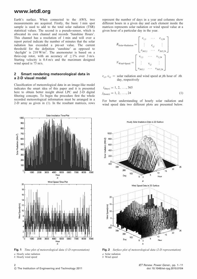
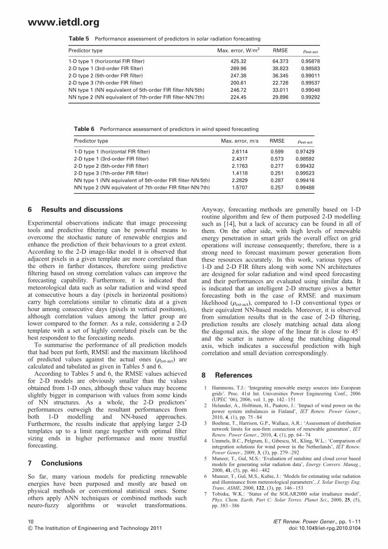
For better understanding of hourly solar radiation andwind speed data two different plots are presented below.

Fig. 1 Time plot of meteorological data (1-D representation)

a Hourly solar radiationb Hourly wind speed

Fig. 2 Surface plot of meteorological data (2-D representation)

a Solar radiationb Wind speed

2 IET Renew. Power Gener., pp. 1–11

& The Institution of Engineering and Technology 2011 doi: 10.1049/iet-rpg.2010.0104

www.ietdl.org

First 1-D representation or time plot of climatic data (Figs. 1aand b) and second the 2-D representation or surface plot ofmentioned information (Figs. 2a and b).

Two remarkable points can be observed from previousfigures. First the periodical behaviour of solar radiationand the stochastic nature of wind speed is obvious fromboth 1-D and 2-D representations, but in the former it istroublesome to make distinction between irradiation andwind speed through different days and hours, whereas thisinterpretation is feasible in the latter. Now to make theimage-like models complete, the surface models shown inFigs. 2a and b must be converted into grey-scale image asshown in Figs. 3a and b. In this image corresponding pixelsrepresented by different grey values that range from whiteto black reveal hourly solar radiation and wind speedinformation in a smart form and this kind of indexedsequential access method guides us to a distinctiveestimation approach via both LPC and 2-D imageprocessing using expert finite impulse response (FIR) filtersas will be explained later.

3 Fundamentals of predictive image filtering

Predictive filtering in the field of image processing is definedas a particular operation in which the scalar value of any givenpixel inside the image range can be calculated by applyingsome mathematical algorithms to the values of the pixels inthe neighbourhood of the target pixel. In this regard, linearpredictive filtering is explained as a common form offiltering in which the output pixel value can be determinedas a linear combination of neighbouring pixels magnitudes.Generally, for a typical LPC we derive an algorithm withtwo separate parts: encoding part and synthesis (decoding)part. In an encoding part, the designed LPC takes the inputsamples in predefined blocks and determines the input time-series signal and related filter taps in order to reproduce thecurrent block of information. These output data arequantised and passed into the second part. In the decodingsection, the filter is reconstructed by LPC based on thereceived coefficients from the previous part. The wholefilter structure can be viewed as a tube that, when is fed byan input signal, produces required information (forecastedvalues). In predictive coding, different types of filters canbe designed and applied to the work, but basically there aretwo kinds of filters: finite impulse response (FIR) filters andinfinite impulse response (IIR) filters. Mostly, the FIR filterfunction is implemented as a direct form structure as shownin Fig. 4 or (2).

y(n) = b(1) × x(n) + b(2) × x(n − 1)

+ · · · + b(nb + 1) × x(n − nb)

− a(2) × y(n − 1) − · · · − a(na + 1) × y(n − na)

(2)

where n 2 1 is the filter order, na is the feedback filter orderand nb is the feed forward filter order. In a general manner,the operation of filter at sample is given by the time domaindifference equations (3)

y(t) =∑n−1

t=0

htx(t − t), t [ Z

x : Z � R is the input signal; y : Z � R is the output signal

hi [ R are called filter coefficients; n is filter order or length

(3)

4 Fundamentals of ANN

As mentioned earlier, because ANN has inherent capabilityfor non-linear functionality and accurate mapping, it canbe applied for prediction objectives. Furthermore, thestochastic nature of renewable energies makes ANNspowerful tools to overcome limitations accompanied bysome conventional linear methods that is, ANNs can betrained wisely to solve any complex problem which is hardto grasp analytically [15]. Generally, the structure of anANN consists of three basic elements: weights, thresholdsand activation function connected by a true learningalgorithm. In this regard, back propagation (BP) is a kind oflearning algorithm which is both simple and applicable[16]. During BP training phase several algorithms can beapplied and a brief description from two of these algorithmsis provided here.

Fig. 3 Rendering meteorological data in a grey-scale-imagemodel

a Solar radiationb Wind speed


www.ietdl.org

4.1 Gradient descent algorithm (basic BPalgorithm)

In gradient descent training algorithm the error function,which carries the halved sum of squares of element-wiseerror terms, is expressed as

1 = 1

2

∑n

k=1

(tk − ok )2

( )(4)

where tk and ok are the target output and real output,respectively, and k is the number of output data. As saidbefore, network weights and biases must be updated in eachepoch and new values are used for subsequent iterations asshown in (5).

W ij(k) = U (k) + m · W ij(k − 1) (5)Q3

where Wij(k) is the current weights and bias vector, U(k) is theupdate function and m is the momentum factor which adds afraction of the previous weights update to the current ones andit is limited between 0 and 1(0 ≤ m ≤ 1). Using gradientdescent algorithm the update function (U(k)) is calculated as

g(k) = m∂1

∂Wij(k)� U (k) = −g(k) (6)

where m is the learning rate which controls the step size whenweights are iteratively adjusted. It is worthy of note that thebasic BP training algorithm works by altering the values ofweights with a fixed length vector in the direction of thenegative gradient to minimise an error function. In thisregard, (4) is valid for the networks that have one outputvector.

4.2 Levenberg–Marquardt algorithm

Levenberg–Marquardt (L–M) algorithm is an iterativesequence of instructions similar to any numericminimisation algorithms and it can find a solution even ifthe target minimum be far away from the start point [17].For L–M algorithm the update function U(k) can becomputed using (7).

U (k) = −[JT × J + b× diag(J T × J )]−1 × J T × 1 (7)

where J is the Jacobian matrix which includes first-orderderivatives of the network errors with respect to the weightsand biases, and 1 is the vector of network errors. b is anon-negative scalar number called damping factor and diagis an abbreviation for diagonal matrix which is equal toidentity matrix in this equation.

5 Designing linear predictive digital FIRfilters

In linear forecasting, future samples or target outputs can beoptimally estimated through an autoregressive process usinga linear combination of past samples. Suppose that thepresent values of the climatic data are predicted by the pastM samples of the related signal such that

x(n) = a1x(n − 1) + a2x(n − 2) + · · · + aM x(n − M )

=∑Mi=1

aix(n − i) (8)

where x(n) is the estimation of x(n), x(n 2 i) is the ith stepprevious sample, and {ai} is regarded as the vector of linearprediction coefficients. The error between the real value andthe estimated one can be expressed as

1(n) = x(n) − x(n) = xn −∑Mi=1

aix(n − i) (9)

To find optimal filter coefficients that best describe the currentplan of action, first the error function must be minimised inthe sense of mean squared error (10).

E =∑

n

12(n) =∑

n

(x(n) −∑Mi=1

aix(n − i))2 (10)

The most accurate tap vector {ai} can be found by minimisingthe sum of the squared error. If the first-order derivative ofE with respect to ai set to zero (using the chain rule), oneobtains

2∑

n

x(n − k) x(n) −∑Mi=1

aix(n − i)

( )= 0

for k = 1, 2, 3, . . . , M (11)

Taking the above derivatives yields M equations that can bewritten as

a1

∑n

x(n − k)x(n − 1) + a2

∑n

x(n − k)x(n − 2)

+ · · · + aM

∑n

x(n − k)x(n − M )

=∑

n

x(n − k)x(n); for k = 1, 2, 3, . . . , M (12)

Suppose that an input signal is divided into several frameseach with N samples. If each frame length is short enough

Fig. 4 Direct form II transposed FIR filter



www.ietdl.org

then the signal in the related frame may be stationary. Itshould be also noted that the signal equals zero out of thecurrent template range. If N samples exist in the sequencecategorised from 0 to N 2 1, {xn} ¼ {x(0), x(1), x(2), . . .,x(N 2 2), x(N 2 1)} then (12) can be stated in terms of amatrix equation as given in (13)

r(0) r(1) r(2) · · · r(M − 2) r(M − 1)

r(1) r(0) r(1) · · · r(M − 3) r(M − 2)

r(2) r(1) r(0) · · · r(M − 4) r(M − 3)

..

. ... ..

. ... ..

.

..

. ... ..

. ... ..

.

r(M − 1) r(M − 2) r(M − 3) · · · r(1) r(0)

⎡⎢⎢⎢⎢⎢⎢⎢⎢⎢⎣

⎤⎥⎥⎥⎥⎥⎥⎥⎥⎥⎦

×

a1

a2

a3

..

.

aM−1

aM

⎡⎢⎢⎢⎢⎢⎢⎢⎢⎢⎣

⎤⎥⎥⎥⎥⎥⎥⎥⎥⎥⎦=

r(1)

r(2)

r(3)

..

.

r(M − 1)

r(M )

⎡⎢⎢⎢⎢⎢⎢⎢⎢⎢⎣

⎤⎥⎥⎥⎥⎥⎥⎥⎥⎥⎦

R · a = r

(13)

where

r(k) =∑N−1−k

n=0

x(n)x(n+ k) (14)

The above calculation is generally called the autocorrelationmethod [18] and if such a method is applied for designing

Fig. 5 Different types of prediction models

a 1-D horizontal predictionb 2-D FIR filterc Equivalent NN of a fifth-order FIR filter (NN/5th)d Equivalent NN of a seventh-order FIR filter (NN/7th)

Table 1 Correlation coefficients between solar radiation data

within the template

ri,j j ¼ 0 j ¼ 1 j ¼ 2 j ¼ 3

i ¼ 0 1 0.94738 0.83410 0.68275

i ¼ 1 0.83428 0.80376 0.71825 0.59514

i ¼ 2 0.81116 0.80191 0.69842 0.57903

i ¼ 3 0.83259 0.79878 0.71644 0.59287

Table 2 Correlation coefficients between wind speed data

within the template

ri,j j ¼ 0 j ¼ 1 j ¼ 2 j ¼ 3

i ¼ 0 1 0.97679 0.93389 0.87019

i ¼ 1 0.87403 0.87051 0.86210 0.84807

i ¼ 2 0.87410 0.86995 0.86103 0.83261

i ¼ 3 0.86651 0.86178 0.84759 0.84582


www.ietdl.org

process the synthesis filter will be stable. To solve the matrixequation and calculate the filter coefficients first it is needed tocompute the inverse of correlation matrix (R21). Since R is asymmetric matrix with similar diagonal elements, theinversion action can be done easily using some recursiveapproaches like Levinson–Durbin (L–D), which iscomputationally efficient while determining the filtercoefficients using (15)

a = R−1r (15)

It should be mentioned that for a time-varying series thecorrelation coefficient (r) between two random variableswith expected values mx and mY and standard deviations sX

and sY is defined as

rX ,Y = Corr(X , Y ) = cov(X , Y )

sXsY

= E[(X −mX )(Y −mY )]

sXsY

(16)

where E is the mathematical expectation, cov(X, Y ) meanscovariance between X and Y variables and Corr is a famousnotation for Pearson’s correlation [18].

5.1 2-D FIR filters against 1-D representations andANNs

To evaluate the performance of the purposed filters differenttypes of structures are designed and tested via similar data.First a horizontal model is created and treated as anexample for conventional 1-D prediction. Then three typesof 2-D FIR filters are constructed and considered as theproposed estimation approach in this paper and finally twoNNs are designed as non-linear predictive models withsimilar input pattern to those of 2-D models. The accuracyof the models is compared in terms of maximum predictionerror, root mean square error (RMSE) and the correlationbetween predicted and actual data (rest2act).

It must be pointed out that in LPC it is proved that a preciseand robust 2-D forecasting process relies on applying highlycorrelated information [19]. The more the correlated dataresults, the less the prediction error and the more theforecasting quality. In this regard, correlation coefficients

between solar radiation and wind speed data within atemplate with four pixels in length and width, showing four

Table 3 Optimal filter taps weights for solar radiation prediction

Q4 Filter type h1 h2 h3 h4 h5 h6 h7

1-D type 1 (horizontal FIR filter) 1.398087 2 0.31506 2 0.17252 N/A∗ N/A N/A N/A

2-D type 1 (3rd-order FIR filter) 1.434167 2 0.37205 2 0.16102 N/A N/A N/A N/A

2-D type 2 (5th-order FIR filter) 1.296368 1.296368 0.080054 0.03978 0.078725 N/A N/A

2-D type 3 (7th-order FIR filter) 1.274913 2 0.52869 0.05721 0.022567 0.058618 0.043943 0.035129

N/A: not available.

Table 4 Optimal filter taps weights for wind speed prediction

Q4 Filter type h1 h2 h3 h4 h5 h6 h7

1-D type 1 (horizontal FIR filter) 0.377694 0.209899 0.361598 N/A∗ N/A N/A N/A

2-D type 1 (3rd-order FIR filter) 0.8716971 0.159227 20.05037 N/A N/A N/A N/A

2-D type 2 (5th-order FIR filter) 0.893364 0.206905 20.08787 0.021717 20.06018 N/A N/A

2-D type 3 (7th-order FIR filter) 0.08103 0.019701 0.048049 0.811706 0.144028 20.07116 20.03866

N/A: not available

Fig. 6 Performance curve of 5th-NN as a function of epochnumbers

a Solar radiation prediction performanceb Wind speed prediction performance



www.ietdl.org

consecutive hours a day and four consecutive days in a yearare tabulated in Tables 1 and 2 using (16).

Conventional forecasting methods are generally based onutilising past samples in a 1-D template that refers to ahorizontal prediction as shown in Fig. 5a. Such a methodcan be found in [20], applying 14, 15, 28 and 29 weathersamples before the hour to be forecasted. It is observedfrom the first rows of Tables 1 and 2 that horizontal pixelsare highly correlated and they can act properly in

forecasting process. Now, the plan of action changes fromformal 1-D approaches to expert 2-D one which takesadvantages from highly correlated information in bothdirections within the template domain. Referring toTables 1 and 2, again it is observed that correlationcoefficients between meteorological data decrease as longas i and j increase across the template and the neighbouringpixels in multiple directions which convey information fromprevious hours and days contain strong correlations with

Fig. 7 Performances of different models in the case of solar radiation and wind speed forecasting

a Solar radiationb Wind speed: 1-D horizontal forecasting performancec Solar radiationd Wind speed: 2-D forecasting performance (third-order FIR filter)e Solar radiationf Wind speed: 2-D forecasting performance (fifth-order FIR filter)g Solar radiationh Wind speed: 2-D forecasting performance (seventh-order FIR filter)i Solar radiationj Wind speed: NN/5th forecasting performancek Solar radiationl Wind speed: NN/7th forecasting performance


www.ietdl.org

Fig. 7 Continued



www.ietdl.org

each other. Therefore considering a set of pixels withthe highest correlations can be a decisive factor forimplementation of expert 2-D FIR filters as shown inFig. 5b. Here, to assess the 2-D forecasting performance bymeans of non-linear functions two NN architectures areadopted and fed by similar data. Each NN is constructed onthe basis of its equivalent 2-D FIR filter mentioned aboveand has multiple inputs chosen from the template domain,similar to those of 2-D models, and a single output relatesto estimated value as shown in Figs. 5c and d. In thisregard, since the input data values and their patterns are thesame in the NNs architectures and the proposed 2-D FIRfilters, the comparison of results are possible and valid.Solar radiation and wind speed data from 10 months of thetypical year are selected randomly for training phase andthe rest are used for testing process. For both networksS-shaped (sigmoidal) activation function is utilised and thepreviously mentioned learning algorithms (gradient descent,L–M) are applied for training phase. The number ofneurons in hidden layer is also determined experimentallythrough a trial and error action.

5.2 Forecasting performance evaluation

In order to assess the performance of purposed FIR filters theexact template size and optimal filter coefficients must becomputed so as to fit the needs. Tables 3 and 4 indicateoptimal tap weights of different 1-D and 2-D filters forsolar radiation and wind speed prediction using (15).

To derive the equivalent NN architectures, first the numberof inputs must meet the requirements. Since we want tocompare the performances in the case of linear and non-linear prediction the input vector must be the same in bothstructures. For example if a FIR filter uses five input pixelswith the highest correlations, known as fifth-order FIRfilter, then the same input data from the same positionsinside the 2-D template are selected for the equivalent NNof that FIR filter (NN/5th).

For better convergence of NNs solar radiation and windspeed data are normalised between 21 and +1 linearly.

Moreover, from various training algorithms two are selectedand compared in terms of prediction error and resemblanceof predicted values to target values. It is observed that L–M algorithm shows better performance, therefore it isapplied for training phase of both networks. It is foundexperimentally that using eight neurons in the hidden layertogether with L–M training algorithm provides the bestperformance and the least prediction error. As an example,Figs. 6a and b show the performance curve for NN/5th as afunction of epochs in the case of solar radiation and windspeed prediction. It is observed from Fig. 6 that duringlearning phase the desired performance is obtained within30 and 15 epochs for solar radiation and wind speedforecasting, respectively, although the learning algorithm isrun 100 epochs for each prediction model.

The performance evaluation of models begins with thehorizontal prediction. A set of data including three samplesfrom previous hours in a same day feeds the predictionmodel and forecasted values are obtained, respectively, asshown in Figs. 7a and b. The second model known asthird-order FIR filters again applies three samples with thehighest correlation but from previous hours and daysconsidering a 2-D template domain. As shown in Figs. 7cand d the forecasting performance improves greatly incomparison with that of horizontal one, although thenumber of input data remains unchanged. In this regard, ifwe extend the 2-D filtering window (up to a limit range)and use more samples from both directions the performanceshows further improvement as shown in Figs. 7e–h.Finally, to assess the prediction performance by means ofnon-linear forecasting two NNs are designed and trainedon the basis of their equivalent 2-D representationsregarding the previously mentioned focal points. Figs. 7i– lindicate the performances of NN/5th and NN/7th in thecase of solar radiation and wind speed forecasting,respectively. It is observed from simulation results, althoughthe performances of NN-based approaches outweigh theones from 2-D FIR predictive filters in low orders (e.g. 5th-order) but different results are achieved in higher orders andbetter performance from the proposed method is observed.

Fig. 7 Continued


www.ietdl.org

6 Results and discussions

Experimental observations indicate that image processingtools and predictive filtering can be powerful means toovercome the stochastic nature of renewable energies andenhance the prediction of their behaviours to a great extent.According to the 2-D image-like model it is observed thatadjacent pixels in a given template are more correlated thanthe others in farther distances, therefore using predictivefiltering based on strong correlation values can improve theforecasting capability. Furthermore, it is indicated thatmeteorological data such as solar radiation and wind speedat consecutive hours a day (pixels in horizontal positions)carry high correlations similar to climatic data at a givenhour among consecutive days (pixels in vertical positions),although correlation values among the latter group arelower compared to the former. As a rule, considering a 2-Dtemplate with a set of highly correlated pixels can be thebest respondent to the forecasting needs.

To summarise the performance of all prediction modelsthat had been put forth, RMSE and the maximum likelihoodof predicted values against the actual ones (rest-act) arecalculated and tabulated as given in Tables 5 and 6.

According to Tables 5 and 6, the RMSE values achievedfor 2-D models are obviously smaller than the valuesobtained from 1-D ones, although these values may becomeslightly bigger in comparison with values from some kindsof NN structures. As a whole, the 2-D predictors’performances outweigh the resultant performances fromboth 1-D modelling and NN-based approaches.Furthermore, the results indicate that applying larger 2-Dtemplates up to a limit range together with optimal filtersizing ends in higher performance and more trustfulforecasting.

7 Conclusions

So far, many various models for predicting renewableenergies have been purposed and mostly are based onphysical methods or conventional statistical ones. Someothers apply ANN techniques or combined methods suchneuro-fuzzy algorithms or wavelet transformations.

Anyway, forecasting methods are generally based on 1-Droutine algorithm and few of them purposed 2-D modellingsuch as [14], but a lack of accuracy can be found in all ofthem. On the other side, with high levels of renewableenergy penetration in smart grids the overall effect on gridoperations will increase consequently; therefore, there is astrong need to forecast maximum power generation fromthese resources accurately. In this work, various types of1-D and 2-D FIR filters along with some NN architecturesare designed for solar radiation and wind speed forecastingand their performances are evaluated using similar data. Itis indicated that an intelligent 2-D structure gives a betterforecasting both in the case of RMSE and maximumlikelihood (rest-act), compared to 1-D conventional types ortheir equivalent NN-based models. Moreover, it is observedfrom simulation results that in the case of 2-D filtering,prediction results are closely matching actual data alongthe diagonal axis, the slope of the linear fit is close to 458and the scatter is narrow along the matching diagonalaxis, which indicates a successful prediction with highcorrelation and small deviation correspondingly.

8 References

1 Hammons, T.J.: ‘Integrating renewable energy sources into Europeangrids’. Proc. 41st Int. Universities Power Engineering Conf., 2006(UPEC ’06), 2006, vol. 1, pp. 142–151

2 Helander, A., Holttinen, H., Paatero, J.: ‘Impact of wind power on thepower system imbalances in Finland’, IET Renew. Power Gener.,2010, 4, (1), pp. 75–84

3 Boehme, T., Harrison, G.P., Wallace, A.R.: ‘Assessment of distributionnetwork limits for non-firm connection of renewable generation’, IETRenew. Power Gener., 2010, 4, (1), pp. 64–74

4 Ummels, B.C., Pelgrum, E., Gibescu, M., Kling, W.L.: ‘Comparison ofintegration solutions for wind power in the Netherlands’, IET Renew.Power Gener., 2009, 3, (3), pp. 279–292

5 Muneer, T., Gul, M.S.: ‘Evaluation of sunshine and cloud cover basedmodels for generating solar radiation data’, Energy Convers. Manag.,2000, 41, (5), pp. 461–482

6 Muneer, T., Gul, M.S., Kubie, J.: ‘Models for estimating solar radiationand illuminance from meteorological parameters’, J. Solar Energy Eng.Trans. ASME, 2000, 122, (3), pp. 146–153

7 Tobiska, W.K.: ‘Status of the SOLAR2000 solar irradiance model’,Phys. Chem. Earth, Part C: Solar Terres. Planet Sci., 2000, 25, (5),pp. 383–386

Table 5 Performance assessment of predictors in solar radiation forecasting

Predictor type Max. error, W/m2 RMSE rest-act

1-D type 1 (horizontal FIR filter) 425.32 64.373 0.95878

2-D type 1 (3rd-order FIR filter) 269.96 38.823 0.98583

2-D type 2 (5th-order FIR filter) 247.38 36.345 0.99011


NN type 1 (NN equivalent of 5th-order FIR filter-NN/5th) 246.72 33.011 0.99048


Table 6 Performance assessment of predictors in wind speed forecasting

Predictor type Max. error, m/s RMSE rest-act

1-D type 1 (horizontal FIR filter) 2.6114 0.599 0.97429

2-D type 1 (3rd-order FIR filter) 2.4317 0.573 0.98592







www.ietdl.org

8 Reddy, K.S., Manish, R.: ‘Solar resource estimation using artificialneural networks and comparison with other correlation models’,Energy Convers. Manage., 2003, 44, pp. 2519–2530

9 Giebel, G., Landberg, L., Kariniotakis, G., Brownsword, R.: ‘State-of-the-art on methods and software tools for short-term prediction ofwind energy production’. Proc. EWEC, Madrid, Spain, 2003

10 Landberg, L., Giebel, G., Nielsen, H.A., Nielsen, T., Madsen, H.:‘Short-term prediction – an overview’, Wind Energy (SpecialReview Issue on Advances in Wind Energy), 2003, 6, (3),pp. 273–280

11 Barbounis, T.G., Theocharis, J.B., Alexiadis, M.C., Dokopoulos, P.S.:‘Long-term wind speed and power forecasting using local recurrentneural network models’, IEEE Trans. Energy Convers., 2006, 21, (1),pp. 273–284

12 Chaabene, M., Ben Ammar, M.: ‘Neuro-fuzzy dynamic model withKalman filter to forecast irradiance and temperature for solar energysystems’, Renew. Energy, 2008, pp. 1435–1443Q5

13 Cao, J.C., Cao, S.H.: ‘Study of forecasting solar irradiance using neuralnetworks with preprocessing sample data by wavelet analysis’, Energy,2006, 3, pp. 13435–13445

14 Hocaoglu, F.O., Gerek, O.N., Kurban, M.: ‘A novel 2-D model approachfor the prediction of hourly solar radiation’, (LNCS 4507), (Springer,2007), pp. 741–749

15 Fausset, L.: ‘Fundamentals of neural networks’ (Prentice-Hall, UpperSaddle River, NJ, 1994)

16 Haykin, S.: ‘Neural networks: a comprehensive foundation’ (Prentice-Hall, Upper Saddle River, NJ, 1999)

17 Levenberg, K.: ‘A method for the solution of certain non-linearproblems in least squares’, Quart. Appl. Math., 1944, 2, pp. 164–168

18 Rodgers, J.L., Nicewander, W.A.: ‘Thirteen ways to look at thecorrelation coefficient’, Am. Statist., 1988, 42, pp. 59–66[doi:10.2307/2685263]

19 Gonzalez, R.C., Woods, R.E.: ‘Digital image processing’ (Prentice-Hall,Englewood Cliffs, USA, 2002, 2nd edn.), pp. 461–463

20 Cao, J., Lin, X.: ‘Study of hourly and daily solar irradiation forecastusing diagonal recurrent wavelet neural networks’, Energy Convers.Manage., 2008, 49, (6), pp. 1396–1406

21 IntersilTM. ‘An introduction to digital filters. Application note’, 1999,AN9603.2. www.intersil.com Q6

22 Douglas, S.C.: ‘Introduction to adaptive filters’. Digital signalprocessing handbook 1999, pp. 7–12 Q7

23 Nelson, M., Gailly, J.-L.: ‘Speech compression’. The data compressionbook 1995, pp. 289–319 Q7

24 Dukpa, A., Duggal, I., Venkatesh, B., Chang, L.: ‘Optimal participationand risk mitigation of wind generators in an electricity market’, IETRenew. Power Gener., 2010, 4, (2), pp. 165–175


www.ietdl.org

www.intersil.com

RPG20100104Author Queries

A. Anvari Moghaddam, A.R. Seifi

Q1 References are renumbered to get the sequence order. Please check

Q2 Please check the sentence “Moreover, since the 2-D modeling. . . information for operators.” for sense clarity

Q3 IET style for matrices and vectors is to use bold italics. Please check that we have identified all instances correctly

Q4 Please provide the significant of asterik (∗) in table body of Tables 3 and 4

Q5 Please provide volume number for Ref. 12

Q6 Refs. 21-24 are not cited in the text. Please cite in the text, else delete from the list

Q7 Please provide publisher name in Ref. [22,23]

www.ietdl.org

Aalborg Universitet Study of Forecasting Renewable ...

Documents

Transcript of Aalborg Universitet Study of Forecasting Renewable ...