Aalborg Universitet Sparse Variational Bayesian SAGE...

Aalborg Universitet

Sparse Variational Bayesian SAGE Algorithm With Application to the Estimation ofMultipath Wireless ChannelsShutin, Dmitriy; Fleury, Bernard Henri

Published in:I E E E Transactions on Signal Processing

DOI (link to publication from Publisher):10.1109/TSP.2011.2140106

Publication date:2011

Document VersionAccepted author manuscript, peer reviewed version

Link to publication from Aalborg University

Citation for published version (APA):Shutin, D., & Fleury, B. H. (2011). Sparse Variational Bayesian SAGE Algorithm With Application to theEstimation of Multipath Wireless Channels. I E E E Transactions on Signal Processing, 59(8), 3609-3623. DOI:10.1109/TSP.2011.2140106

General rightsCopyright and moral rights for the publications made accessible in the public portal are retained by the authors and/or other copyright ownersand it is a condition of accessing publications that users recognise and abide by the legal requirements associated with these rights.

? Users may download and print one copy of any publication from the public portal for the purpose of private study or research. ? You may not further distribute the material or use it for any profit-making activity or commercial gain ? You may freely distribute the URL identifying the publication in the public portal ?

Take down policyIf you believe that this document breaches copyright please contact us at [email protected] providing details, and we will remove access tothe work immediately and investigate your claim.

Downloaded from vbn.aau.dk on: June 14, 2018

https://doi.org/10.1109/TSP.2011.2140106

http://vbn.aau.dk/en/publications/sparse-variational-bayesian-sage-algorithm-with-application-to-the-estimation-of-multipath-wireless-channels(a169caef-004d-4a52-af04-d09a241af9c3).html

IEEE TRANSACTIONS ON SIGNAL PROCESSING, VOL. 59, NO. 8, AUGUST 2011 3609

Sparse Variational Bayesian SAGE AlgorithmWith Application to the Estimation of

Multipath Wireless ChannelsDmitriy Shutin, Member, IEEE, and Bernard H. Fleury, Senior Member, IEEE

Abstract—In this paper, we develop a sparse variationalBayesian (VB) extension of the space-alternating generalized ex-pectation-maximization (SAGE) algorithm for the high resolutionestimation of the parameters of relevant multipath componentsin the response of frequency and spatially selective wirelesschannels. The application context of the algorithm consideredin this contribution is parameter estimation from channelsounding measurements for radio channel modeling purpose.The new sparse VB-SAGE algorithm extends the classical SAGEalgorithm in two respects: i) by monotonically minimizing thevariational free energy, distributions of the multipath componentparameters can be obtained instead of parameter point estimatesand ii) the estimation of the number of relevant multipathcomponents and the estimation of the component parametersare implemented jointly. The sparsity is achieved by definingparametric sparsity priors for the weights of the multipathcomponents. We revisit the Gaussian sparsity priors withinthe sparse VB-SAGE framework and extend the results byconsidering Laplace priors. The structure of the VB-SAGEalgorithm allows for an analytical stability analysis of the updateexpression for the sparsity parameters. This analysis leads tofast, computationally simple, yet powerful, adaptive selectioncriteria applied to the single multipath component considered ateach iteration. The selection criteria are adjusted on a per-com-ponent-SNR basis to better account for model mismatches, e.g.,diffuse scattering, calibration and discretization errors, allowingfor a robust extraction of the relevant multipath components.The performance of the sparse VB-SAGE algorithm and itsadvantages over conventional channel estimation methods aredemonstrated in synthetic single-input–multiple-output (SIMO)time-invariant channels. The algorithm is also applied to realmeasurement data in a multiple-input–multiple-output (MIMO)time-invariant context.

Manuscript received March 23, 2010; revised September 17, 2010 and Feb-ruary 24, 2011; accepted March 16, 2011. Date of publication April 07, 2011;date of current version July 13, 2011. The associate editor coordinating thereview of this manuscript and approving it for publication was Dr. Mark Coates.This work was supported in part by the Austrian Science Fund (FWF) byGrant NFN SISE (S106), by the European Commission within the ICT-216715FP7 Network of Excellence in Wireless Communications (NEWCOM++), bythe project ICT-217033 Wireless Hybrid Enhanced Mobile Radio Estimators(WHERE), and by the project ICT-248894 (WHERE-2).

D. Shutin is with the Department of Electrical Engineering, Princeton Uni-versity, B311 E-QUAD, Princeton NJ 08544 USA (e-mail: [email protected]).

B. H. Fleury is with the Section Navigation and Communications, Depart-ment of Electronic Systems, Aalborg University, DK-9220 Aalborg, Denmark(e-mail: [email protected]).

Color versions of one or more of the figures in this paper are available onlineat http://ieeexplore.ieee.org.

Digital Object Identifier 10.1109/TSP.2011.2140106

Index Terms—Expectation-maximization algorithm, MIMO,multipath channels, SAGE algorithm, variational Bayesianmethods.

I. INTRODUCTION

I N modeling real world data, proper model selection playsa pivotal role. When applying high resolution algorithms

to the estimation of wireless multipath channels from multidi-mensional channel measurements, an accurate determinationof the number of dominant multipath components is requiredin order to reproduce the channel behavior in a realisticmanner—an essential driving mechanisms for the design anddevelopment of next generation multiple-input–multiple-output(MIMO)-capable wireless communication and localizationsystems. Consider for simplicity a single-input–multiple-output(SIMO) wireless channel,1 e.g., an uplink channel with a basestation equipped with multiple antennas. The received signalvector made of the signals at the outputs of these antennascan be represented as a superposition of an unknown numberof multipath components contaminated by additivenoise [1]

(1)

In (1) is the multipath weights and is the received ver-sion of the transmitted signal modified according to the disper-sion parameter vector of the th propagation path.2 Classicalparameter estimation [2]–[5] deals with the estimation of themultipath components, i.e., and , while the estimation ofthe number of these components is the object of model order

1The proposed method can be easily extended to MIMO time-variant channelswith stationary propagation constellation. With minor modifications the polar-ization aspects can be included as well. This extension merely leads to a morecomplicated signal model, including for instance more dispersion parameters,without adding any new aspect relevant to the understanding of the new pro-posed concepts and methods. The scenario considering a SIMO channel seemsa sensible compromise between complexity of the model underlying the the-oretical analyses and an interesting application in which the proposed methodcan be demonstrated. However, in the experimental section we consider the es-timation of a MIMO channel.

2We mean as dispersion parameters of the waves propagating from the trans-mitter side to the receiver site—and, by generalization, of the multipath compo-nents in the resulting channel response—their relative delay, direction of depar-ture, direction of arrival, and Doppler frequency. The parameter �� includes allthese parameters or a subset of them depending on the transmitter and receiverconfigurations.

1053-587X/$26.00 © 2011 IEEE

3610 IEEE TRANSACTIONS ON SIGNAL PROCESSING, VOL. 59, NO. 8, AUGUST 2011

selection [6]–[9]. Despite its obvious simplicity, (1) provides anoversimplified description of reality: it adequately accounts forspecular-like propagation paths only. Components originatingfrom diffuse scattering inevitably present in measured channelresponses are not rendered appropriately in (1). More specifi-cally, a very large number of specular components is neededto represent such diffuse components. Further effects leading tomodel mismatch are errors in calibration of the response of thetransceiver or measurement equipment that cause inaccuraciesin the description of , as well as the discrete-time ap-proximation to (1), typically arising when model parameters areestimated using numerical optimization techniques. All theseeffects have a significant impact on the performance of boththe parameter estimation algorithms and the model order se-lection schemes derived based on (1). Experimental evidenceshows that if the model order selection scheme is not carefullydesigned, the above model mismatch will lead to an overestima-tion of the number of relevant multipath components. Fictivecomponents without any physical meaning will be introducedand their parameters estimated. Hence, radio channel estima-tors combining model order (component number) selection andcomponent parameter estimation that are robust against modelmismatch are needed here.

Bayesian methods are promising candidates for such robustmethods. For a fixed model order the classical maximum like-lihood (ML) approach to the estimation of dispersion parame-ters and gains in (1)involves maximization of the multidimensional parameter like-lihood given the measurement . Although efficientalgorithms exist to solve this optimization problem [2], [3], [10],standard ML algorithms require a fixed number of components

and typically do not employ any likelihood penalization tocompensate for overfitting. Bayesian techniques can compen-sate for this through the use of a prior , which effec-tively imposes constrains on the model parameters. The modelfit (i.e., the value of the likelihood) can be traded for the modelcomplexity [i.e., number of components in (1)] through the like-lihood penalization. Likelihood penalization lies in the heart ofcelebrated information-theoretic model order selection criteria,such as minimum description length (MDL), Bayesian informa-tion criterion (BIC), as well as their variants [7]–[9].

Imposingconstraintson themodelparameters isakey tosparsesignal modeling [11]–[16]. In Bayesian sparsity approach [11],[13], [14], [17] the gains are constrained using a parametricprior , where is a circularlysymmetric probability density function (pdf), with the priorparameter —also called sparsity parameter—being inverselyproportional to the width of the pdf. Such form of the prior allowsfor controlling the contribution of each basis associated with theweight through the sparsity parameter : a large value ofwill drive the corresponding weight to zero, thus realizing asparse estimator. The sparsity parameters are found as the max-imizers of , which is also known as a type-II likelihoodfunction or model evidence [13], [14], [18] and the correspondingestimation approach is known as the evidence procedure (EP)[14].

In general, evaluating is difficult. This, however, canbe done analytically [11], [13], [14], [17] in the special case

of linear models3 with both model distribution andsparsity prior being Gaussian. This choice of the prior pdf cor-responds to the -type of parameter constraints. Moreover, itcan be shown [19] that in the Gaussian prior case the maximumof the model evidence coincides with the Bayesianinterpretation of the normalized ML model order selection [7]and reduces to the BIC as the number of measurement samplesgrows. Therefore, the EP allows for joint model order selectionand parameter estimation. This approach was investigated in[19] within the context of wireless channels; however, [19]considers the estimation of multipath gains only, thus bypassingthe estimation of the dispersion parameters in (1). Recently,several investigations have been dedicated to study the -typeof parameter penalties [12], [15], [16], [20], [21], which, inthe Bayesian sparsity framework, is equivalent to choosing

as a Laplace prior for . Compared toGaussian priors, such form of constraints leads to sparsermodels [13], [15], [22], [23]. The -type of penalties signifi-cantly limits the analytical study of the algorithm; nonethelessfor models linear in their parameters different efficient nu-merical techniques have been developed [15], [24], [25]. Theextension of the Bayesian sparsity methods with Laplace priorsapplied to the estimation of multipath wireless channels hasnot been explored yet, mainly due to the nonlinearity of thechannel model in . This can be circumvented by using virtualchannel models [16], [21], which is equivalent to a samplingor gridding of the dispersion parameters at the Nyquistrate [16]. The algorithm then estimates the coefficients on thegrid using sparsity techniques [12], [16], [21]. This approach,however, does not provide high resolution estimates of themultipath parameters. Although it is very effective in capturingchannel energy, recent investigations [26] demonstrate thatthis approach inevitably leads to a mismatch between the truechannel sparsity and the estimated sparsity; more specifically,even when fine quantization of is used, the number of virtualmultipath components will always exceed the true number ofmultipath components; in that respect the channel estimatesderived based on virtual models are not appropriate when thegoal is to extract physical multipath components. In this paperwe aim to demonstrate that the superresolution property shouldnot be sacrificed to the linearity of the estimation problem. Weachieve this by: i) casting a super-resolution SAGE algorithmfor multipath parameter estimation [3] in a Bayesian frame-work, and treating the entries in as random variables whosepdfs are to be estimated and ii) combining this estimationscheme with the Bayesian sparsity techniques, as aforemen-tioned, i.e., using multiple sparsity parameters to controlthe model sparsity on a per-component basis. Moreover, as wewill show, our analysis also allows for defining ways to reducethe impact of estimation artifacts due to the basis mismatchesthrough a detailed analysis of the estimation expressions for thesparsity parameters.

Our main contribution in this paper is twofold. First, inorder to realize Bayesian sparse estimation and to overcomethe computational difficulties due to the nonlinearity of the

3In our context this corresponds to assuming �� as known or fixed, and thus�� .

SHUTIN AND FLEURY: SPARSE VB SAGE ALGORITHM 3611

channel model, we propose a new variational Bayesian (VB)[27] extension of the space-alternating generalized expecta-tion-maximization (SAGE) algorithm for multipath parameterestimation [3], [28]. We coin this extension the variationalBayesian SAGE (VB-SAGE). In contrast to the SAGE algo-rithm, the VB-SAGE algorithm estimates the posterior pdfs ofthe model parameters by approximating the true posterior pdf

with a proxy pdf such as to minimizethe variational free energy [27]. Similar to the original SAGEalgorithm [28], the VB-SAGE algorithm relies on the conceptof the admissible hidden data—an analog of the complete datain the EM framework—to optimize at each iteration the vari-ational free energy with respect to the pdfs of the parametersof one component only. We demonstrate that the monotonicityproperty of the VB-SAGE algorithm guarantees that suchoptimization strategy necessarily minimizes the variational freeenergy. Such optimization strategy makes the estimation of theparameters in a tractable optimization problem due to thereduced dimensionality of the resulting objective functions.Second, we demonstrate that the admissible hidden data alsopermits a detailed analytical study of the sparsity parameters

, which leads to selection criteria applied individually to themultipath component updated at each iteration. On the onehand, these selection criteria allow for a fast implementationof the sparse channel estimator; on the other hand, they areeasy to interpret and can be adjusted to compensate for modelmismatch due to, e.g., calibration and discretization errors.Thus, the sparse VB-SAGE algorithm jointly implements theestimation of the number of relevant multipath components andthe estimation of the posterior pdfs of the component parame-ters. We revisit and extend the Gaussian prior case, and presentnew results for Laplace sparsity priors within the framework ofthe VB-SAGE algorithm. It should also be mentioned that theperformed analysis of the sparsity parameters is equally validfor the problem of sparse estimation of virtual channel models[16] with the VB-SAGE algorithm. However, the applicationof the sparse VB-SAGE algorithm to the estimation of virtualchannel models is outside the scope of the paper.

The paper is organized as follows: In Section II we intro-duce the signal model; Section III addresses the derivation of theVB-SAGE algorithm for the multipath parameter estimation,followed by the analysis of the sparsity priors for model orderselection discussed in Section IV; in Section V several practicalissues, e.g., algorithm initialization, are discussed; in Section VIestimation results obtained from synthetic and measured dataare presented; finally, we conclude the paper in Section VII.

Through the paper we shall make use of the following nota-tion. Vectors are represented as boldface lowercase letters, e.g.,

, and matrices as boldface uppercase letters, e.g., . For vec-tors and matrices and denote the transpose and Hermi-tian transpose, respectively. Sets are represented as calligraphicuppercase letters, e.g., . We use to denote an index set, i.e.,

. The assumed number of elements in is , un-less stated otherwise. We will write as a short-hand notation for a list of variables with indices . When

is a set and , then is the complementof in . Similarly, and .Two types of proportionality are used: denotes ;

denotes and thus for some ar-bitrary constants and . An estimate of a random variableis denoted as . We use to denote the expectationof a function with respect to a probability density ;similarly, denotes the expectation with respect tothe joint probability density of the random variables inthe set . Finally, denotes a multivariate com-plex Gaussian pdf with a mean and a covariance matrix ;

denotes a gamma pdf with parameters and .

II. SIGNAL MODEL

Channel sounding is an instrumental method for the design ofaccurate and realistic radio channel models. Channel soundingis usually performed by sending a specific sounding sequence

through the channel and observing the response at thereceiving side. The received signal is then used to estimatethe channel impulse response (CIR) or its parameters when aparametric model of the response is specified. Consider now aSIMO channel model and time-domain channel sounding. Thesounding signal consists of periodically repeated burstwaveforms , i.e., , where hasduration and is formed as

. The known sounding sequence consists ofchips and is the shaping pulse of duration , with

. We assume that the signal vector has beenreceived/measured with an antenna array consisting of sen-sors located at positions with respect toan arbitrary reference coordinate system. The signal originatingfrom the th propagation path is an altered version of the originaltransmitted signal weighted by a complex gain . The al-teration process is described by a (nonlinear) mapping

, where is the vector of dispersion parameters, e.g.,relative delay, azimuth and elevation angles of arrival. The non-linear mapping includes the system effects, e.g.,the transmitter and receiver RF/IF filters and the responses of thetransmit and receive arrays. In the sequel we try to abstract fromthe concrete channel structure where it is possible and keep themodel in its most general form. Additive noise is assumedto be a zero-mean spatially white and temporally wide-sensestationary Gaussian process, i.e., ,and , , , .In our framework we assume that is known.4 In practice

is low-pass filtered and sampled with the sampling period, resulting in -tuples with being the number of output

samples per sensor. By stacking the sampled outputs of thesensors in one vector , (1) can be rewritten as

(2)

where we define ,

, with, and ,

. Finally, we define .

4Although it is possible to reformulate the algorithm to estimate the noisecovariance [14], [29], we will leave this aspect outside the scope of this work.


Fig. 1. (a) Graphical model representing (2) with � components. (b) Extendedmodel with the admissible hidden data �� .

The probabilistic graph depicted in Fig. 1(a) encodes the de-pendencies between the parameters and the observation vectorin the model (2). As visualized in the graph structure, the jointpdf of the probabilistic model can be factored as

, where is the vectorcontaining the model sparsity parameters. Let us now specifythe statistical model behind the involved variables.

Under the Gaussian noise assumption,, with . The second

term is the parameter prior. We assume that, where is the sparsity

prior for the th component. The purpose of the sparsity prioris, on the one hand, to constrain the gains of thecomponents, and thus implement sparsification/model orderselection, and, on the other hand, to control this constraintthrough the sparsity parameters . We will study two choicesfor : i) a Gaussian prior, and ii) a Laplace prior. In bothcases the prior pdfs are complex circularly symmetric, with thenonnegative hyperparameter inversely proportional to theirwidth. Thus, large values of will render the contribution ofthe component “irrelevant” since the correspondingprior over will then be concentrated at the origin. The choiceof the prior is arbitrary; however, it must reflect the under-lying physics and restrictions of the measurement equipment;a non-informative prior can also be used. The prior ,also called the hyperprior of the th component, is selected

as a gamma pdf .Practically we set for all components to rendertheir hyperprior non-informative [13], [14]. Such formulationof a hyperprior pdf is related to automaticrelevance determination [18], [30].

III. PARAMETER ESTIMATION FRAMEWORK

Direct evaluation of or of the posteriorfor performing inference of the unknown parameters is anontrivial task. Two main reasons for this are the nonlinearity ofthe model (1) and the statistical dependence of multipath com-ponent parameters when is observed.5 Approximative tech-niques might significantly ease the model fitting step. In ourwork we resort to the variational Bayesian inference framework.The variational Bayesian inference generalizes the classical EMalgorithm [27] and provides a tool for estimating distributions of

. Essentially, variational methods approximate the poste-rior pdf of interest with a simpler pdf (by, e.g., neglecting somestatistical dependencies between random variables) such that the

5Such graph structure is also referred to as a V-structure [31], which leadsto the conditional dependence of the parent variables when the correspondingchild variable is observed.

Kullback-Leibler divergence between the former pdf and thelatter is minimized.

When estimating parameters using the SAGE algorithm [3],[28], the concept of complete data in the EM algorithm is re-placed by that of admissible hidden data. The purpose of the ad-missible hidden data is to make the update procedure for only asubset a tractable optimization problem. For the vari-able to be an admissible hidden data with respect tothe following factorization must be satisfied:

[28]. The fact that is anadmissible hidden data guarantees that the likelihood of the newparameter update (obtained by replacing the updated pa-rameter subset in the overall parameter set ) cannot besmaller than the likelihood prior to the update [28]. This prop-erty is referred to as the monotonicity property. The conceptof admissible hidden data can be exploited within the varia-tional framework as well. As we will show later, this similarlyleads to an iterative algorithm—we call it the VB-SAGE algo-rithm—that still exhibits the monotonicity property in terms ofthe variational free energy [27].

Consider for a specific component the new variable

(3)

which can be conceived as a received signal associated with theth propagation path. The additive noise component in (3)

is obtained by arbitrarily decomposing the total noise suchthat and . We define

to be the part of the total additive noise that isnot associated with the th component. Thus, . Con-sider now the modified graph in Fig. 1(b) that accounts for . Itis straightforward to show that is an admissible hidden datawith respect to the subset . Since we are interestedin estimating all components, we can formulate the estima-tion algorithm as a succession of estimations ofwith respect to , , assuming that ,

, are known and fixed. According to the extended graphin Fig. 1(b), the joint pdf now factors as

(4)

where

(5)and .

A. Variational Bayesian Inference of Signal Parameters

Variational Bayesian inference [27] is a family of techniquesthat exploit analytical approximations of the posterior pdf of in-terest, i.e., , using a simpler proxy pdf . Thelatter pdf is estimated as a minimizer of the variational free en-ergy [27], which is formally equivalentto the Kullback-Leibler divergencebetween the proxy pdf and the true joint pdf. The admissible


hidden data, used in the SAGE algorithm to facilitate the max-imization of the parameter likelihood, can also be used withinthe variational inference framework to ease the minimization ofthe variational free energy. Such algorithm we term a VB-SAGEalgorithm.

Essentially, the VB-SAGE algorithm approximateswith a variational proxy pdf

(6)

by minimizing the free energy with respect to the parameterof the th component only, and cycling through all compo-nents in a “round-robin” fashion. The monotonicity property ofthe VB-SAGE algorithm (see Appendix A) ensures that suchsequential optimization necessarily decreases the free energy

.It is straightforward to show that with the factorization (6) the

estimation of any factor , , requires theMarkov blanket [31] of to be known.6 Define now

(7)

The unconstrained solution for that minimizes the corre-sponding free energy is then simply found as .Clearly, an unconstrained solution is preferred. However, wemight have to constrain to belong to some class ofpdfs in order to make the optimization tractable. In this case theapproximate solution is obtained by solving

(8)

In the case of it is straightforward to show that isquadratic in ; therefore is a Gaussian pdf, and

. We stress that the constraintguarantees the monotonicity of the VB-SAGE algorithm, as weshow in the Appendix A. Similarly, we select as the setof Gaussian pdfs, i.e., ; notice that

only when is a Gaussian pdf. For thesparsity parameters we select as the set of gammapdfs, i.e., . This choice is dictated by theGamma distribution being the conjugate prior for the inversevariance of the normal distribution; as a result, in the Gaussianprior case . We select as the set of Diracmeasures on the range of ; thus, . By doingso we restrict ourselves to point estimates of the dispersion pa-rameters.7 The parameters , , , , , , and are calledvariational parameters. Obviously, knowing the pdftranslates into knowing the variational parameters of its factorsand vice-versa.

6For a given Bayesian network with � variables, a Markov Blanket of avariable � is the smallest subset of variables �� that “shields”� from the rest of the variables � � � � �� in the sense that�� .

7Considering more complex forms of �� would require the expectation of�� with respect to �� to be evaluated in the closed form. A detailed study ofthis case is outside the scope of this paper.

B. Variational Estimation Expressions

Just like SAGE, the VB-SAGE algorithm is implemented in asequential manner. For the model with signal components thealgorithm sets and updates the proxy factors , ,

, and related to the first component, i.e., updatesthe corresponding variational parameters, based on the currentlyavailable estimates of the factors, i.e., the variational parame-ters, of all other components. In the same fashion thevariational parameters of the component are updated, andso on, until all components are considered. The procedure ofupdating all parameters of all components in this way consti-tutes a single update cycle of the algorithm. The update cyclesare repeated anew until convergence.

In what follows, we consider the update expressions for thevariational parameters of the th com-ponent only. The updated value of a parameter will be denotedby ; let us point out that after has been updated, theother factors related to the component can be updated in anyorder.

1) Estimation of : From the graph in Fig. 1(b), weconclude that . Evaluating (7) in thiscase leads to . Sincethe right-hand side is a product of Gaussian pdfs, is aswell a Gaussian pdf with the mean and covariance matrix givenby

(9)

Thus, . The result (9) general-izes that obtained in [3] by accounting for the covariance matrixof and the noise covariance matrix . Note, however, that theexpression for the mean in (9) is identical to that obtained inthe SAGE algorithm.

Let us consider the limiting case as . It has been shownthat for models linear in their parameters the choiceleads to a fast convergence of the algorithm already in the earlyiteration steps [28]. This is equivalent to assuming that

, which was also used as an admissible

hidden data in [3]. In this case , so that collapsesto a Dirac distribution and .

2) Estimation of : The Markov blanket of is. Here the estimation algorithm profits

from the usage of the admissible hidden data . Since, finding reduces to the computa-

tion of that maximizes given by (7). By noting thatwe obtain

(10)

Notice that due to being a Gaussian pdf within theVB-SAGE framework, (10) includes a Tikhonov-like regular-ization term with the posterior varianceof acting as a regularization constant. Unfortunately, since


depends nonlinearly on , (10) has to be optimizednumerically, e.g., using successive line searches where eachelement of is determined separately or using a joint searchin which all elements of are computed jointly; if derivativesof the objective function (10) with respect to are available,gradient-based optimization schemes can also be used.

Typically is selected to factorize according to, where is the number of dispersion param-

eters describing a multipath component.8 Estimatingcan be done by evaluating (7) using

and performing a simple line search of theresulting objective function. Notice that the same assumptionunderpins the SAGE-based estimation of . The VB-SAGE es-timation expression for in (10) coincides with that of the stan-dard SAGE when is selected non-informative and

.3) Estimation of : The Markov blanket for

is . Evaluating (7) leads to. For a given choice of

the moments of can be either foundin closed form or efficiently approximated. We defer the esti-mation of these moments to Section IV, where different priors

are discussed.4) Estimation of : Here . Observe that

in contrast to and , the admissible hidden data isnot in . This is the result of the Markov chain

; in fact, is the admissible hidden data for estimatingsince due to the fac-

torization (4). By noting that , (7) canbe rewritten as . Dueto the fact that , the variational parame-ters and are found by equating the moments of and

. Observe that it is the estimation of that eventuallyleads to the sparse VB-SAGE algorithm. Also notice that thesparsity prior is a key to the estimation of the sparsityparameters. In the following section, we will consider severalchoices of and analyze their effect on sparsity-basedmodel order selection.

IV. SPARSITY PRIORS FOR MODEL ORDER SELECTION

In this section we consider three choices for the sparsity prior: i) a Gaussian prior, which leads to the -type of log-

likelihood penalty; ii) a flat prior, obtained as a limiting case ofthe Gaussian prior when ; and iii) a Laplace prior, whichresults in the -type of log-likelihood penalty.

A. Gaussian Sparsity Prior

The Gaussian sparsity prior is obtained by selecting. With this choice it is straightfor-

ward to show that and that

(11)

8If some of the dispersion parameters are statistically dependent, a structuredmean field approximation can be used to account for this dependency by meansof an appropriate factorization of the proxy pdf �� .

Observe that (11) is merely a regularized least-squares estimateof given and with the regularization parameter

.The variational parameters and of are found from

. This requires the expectation of to be computed.Doing so leads to the following update expressions:

(12)

Let us now analyze (12) in more details for the case ,i.e., when is non-informative. In this case the mean of

is given as

(13)

Note that this result coincides with the EM-based evidence es-timation proposed in [11] and [14]. However, in our case both

and are estimated using the admissible hidden data , asopposed to [11] and [14] where the incomplete data is usedto obtain these estimates. The updating steps in (11) and (13)can be alternatively repeated, while keeping and fixed togenerate a sequence , where , ,etc. Note that this updating process makes sense since neithernor are in .9 Therefore, the corresponding sequenceof pdfs necessarily mono-

tonically decreases the variational free energy. Let be thestationary point of the sequence when . In

order to simplify the notation we define . By substi-tuting (11) into (13) and solving for we obtain (see also[19])

(14)

By definition , which is satisfied if, and only if,

(15)

By interpreting (13) as a nonlinear dynamic mapping, which atthe iteration maps into , it can be shown [19] that

for the fixed point of the mapping isat infinity, i.e., . As a result, the th signal componentcan be removed from the model.10 A similar result was reportedin [17] using a non-variational analysis of the marginal log-like-lihood function. This allows us to implement model order se-lection during a parameter update iteration, (i.e., joint multipathcomponent detection and parameter estimation, while still min-imizing the variational free energy.

Now, let us reinspect (15). This inequality might at first glanceseem a bit counter-intuitive—the quadratic quantity on the right-hand side is compared to the fourth-power quantity on the left-

9Notice that this property allows for a straightforward extension of the sub-sequent analysis to the estimation of sparse virtual channel models [16] since itremains valid even when the dispersion parameters �� are constrained to someresolution grid.

10Strictly speaking, this is true only in the case of a non-informative hyper-prior �� .


hand side (LHS). In order to better understand the meaning of

it, let us divide both sides of (15) by . Itfollows that (15) is equivalent to

(16)

where . The LHS term in (16) is an

estimate of the posterior variance of scaled by . This resultleads directly to several important observations:

1) The sparsity parameter of the signal component withsmaller than its posterior variance scaled by

is infinite. Thus, such components can be removed fromthe model.

2) By multiplying both sides of (16) with , we findthat this inequality is equivalent to , where

is the estimated signal-to-noiseratio (SNR) of the th component. Thus, (15) [and(16)] corresponds to keeping this component provided

.3) Condition (15) can be tuned to retain the component pro-

vided its estimated SNR is above some predefined levelusing the modified condition

(17)

These results provide us with the required instruments to de-termine whether a component with the sparsity parametershould be updated or pruned: if the component fails to satisfy(15), it is removed since for , . In case of(17) we remove the component if its estimated SNR is belowsome level . Notice that the obtained results allowfor an interpretation of the sparsity parameter in terms ofestimated SNR of the th component. Thus, model order selec-tion (sparsification) can be realized using simple SNR-guideddecisions. It should be stressed that the analysis of (14) is pos-sible only due to the use of the admissible hidden data . Astandard approach with Gaussian priors [11], [14], [17] requiresan posterior covariance matrix of the gain coefficientvector to be computed. This significantlycomplicates the analytical computation of the fixed pointand its analysis. The sparse VB-SAGE algorithm with Gaussiansparsity prior and model order selection scheme that utilizes(15) or (17) we denote as the VB-SAGE-G algorithm.

B. Flat Sparsity Prior

In the case where is chosen to be non-informative,we can still make use of the Bayesian sparsity to estimate themodel order. This can be done by using the VB-SAGE-G algo-rithm in the limiting case as (i.e., ). Due to thestructure of the graph [see Fig. 1(b)], this will only affect themoments of , which remain identical to (11) with .Clearly, in this case and (16) corresponds to the spar-sification of the th component provided , i.e., wekeep the component when its SNR is above 0 dB. The sparse

VB-SAGE algorithm with such model order selection schemewe denote as the VB-SAGE-F algorithm. Observe that (17) canalso be used in the case of the VB-SAGE-F algorithm.

C. Laplace Sparsity Prior (Soft Thresholding)

As the last choice we consider a Laplace prior . Wewill use an analogous Laplace prior in the complex domain de-fined as

(18)

The mean of can be obtained in closed form:

(19)

Here is the sign function defined as . Ex-pression (19) is also known as a soft thresholding rule. To ourbest knowledge no closed form expression for the posterior vari-ance exists. However, we can approximate it with the result ob-tained for the real-valued , which is given as

(20)

Now we turn to the estimation of the sparsity param-eter . By plugging (18) in the expression for ,and ignoring terms independent of , we obtain

. Since is Gaussian,follows a Rice distribution characterized by the parameters

(19) and (20). The expectation is then given

as , where denotes the Laguerre

polynomial with degree . To simplify the estimation of ,

we consider an approximation of as .This approximation is equivalent to assuming a high precisionestimate of . In this case . Then, it isstraightforward to show that

(21)

By selecting a non-informative prior , the update expres-

sion for the mean simplifies to

(22)

Similar to the Gaussian prior case we analyze the fixed pointof (22). We define to simplify the notation.

Combining (22) and (19) leads to

(23)


Assuming that (otherwise ), wesolve for . Doing so yields two solutions:

(24)

(25)

where . Furthermore, we seethat a necessary and sufficient condition for the fixed points tobe real is that

(26)

Components that do not satisfy (26) are removed. Note that bothfixed points are feasible. We have always empirically observedthat when the initial is chosen such that , itera-tions (22) either diverge or converge to the closest(smallest) feasible solution given by (25). The properties of thesecond stationary point are subject to further investigations leftoutside the scope of this paper. The sparse VB-SAGE algorithmwith Laplace sparsity priors that makes use of (26) for modelorder selection we denote as the VB-SAGE-L algorithm.Similarly to (16) it can be shown that (26) is equivalent to

(27)

with . In the same way, (26) and (27)

are equivalent to keeping the component provided ,

where is the estimated componentSNR. Note that (26) and (27) are the Laplace-prior equivalentconditions of (15) and (16) respectively for the Gaussian prior.Although the pruning conditions are formally similar, theydiffer in their numerical values: the moments of areestimated differently computed in these two schemes; as aresult, the estimates of the admissible hidden data for theVB-SAGE-L and VB-SAGE-G algorithms are also different;in addition, the scaling factor in (27) is computed differentlyfrom that in (16). It should also be mentioned that asthe VB-SAGE-L algorithm converges to the VB-SAGE-Falgorithm.

Similarly to (17), (26) can be tuned to keep the componentwhen its estimated SNR is above some predefined level

using the modified condition

(28)

V. IMPLEMENTATION AND INITIALIZATION OF THE ALGORITHM

A. Summary of the Algorithm

Let us now summarize the main steps of the proposed algo-rithm. For the moment we assume that at some iteration the

proxy factors , , , and , , areknown for the components. A single update iteration for thecomponent is summarized in Algorithm 1.

Algorithm 1: Update iteration for the component

Update from (9)

Update from (10) and evaluate

if Condition (17) or (28) are TRUE then

Update from (14) (VB-SAGE-G) or (25)(VB-SAGE-L)

Update from (11) (VB-SAGE-G, -F) or (19)(VB-SAGE-L)

else

Remove the th component;

end if

This update iteration is repeated for all components in around-robin fashion, which constitutes a single update cycleof the algorithm. The update cycles are then repeated untilthe number of components and their variational parametersconverge. Observe that the number of components might bereduced during one update cycle: at each iteration the updatedmultipath component undergoes a test specified by (17) or (28).When the corresponding condition is not satisfied the compo-nent is removed. The model order might also be increased byadding new components. Details of this procedure are outlinedin Section V-D.

B. Algorithm Initialization

We propose a simple bottom-up initialization strategy, whichallows us to infer the initial variational parameters from theobservation by starting with an empty model, i.e., assumingall variational parameters to be 0. The first component isinitialized by letting and applying the initializationloop shown in Algorithm 2. Observe that using the disper-

sion parameters are initialized using a simple beamformer

and the obtained estimate of is plugged in (15) (in theGaussian prior case) or in (26) (in the Laplace prior case) todetermine whether the initialized component should be keptin the model. When the test fails, the initialization stops. Itshould be stressed that the use of (15) or (26) during theinitialization is optional and may be omitted if an overcom-plete channel representation is desired. The components withlarge sparsity parameters will then be pruned later during theupdate iterations. This initialization strategy is similar to thesuccessive interference cancellation scheme proposed in [3]and [5]. The number of initialization iterations (i.e., the initialnumber of signal components) can be either fixed to ,or inferred automatically by repeating the initialization itera-tions until the pruning condition (15) [or (26)] fails at some


iteration.11 In our implementation of the algorithm, we usea combination of the two methods by limiting the maximumnumber of initial components to . The application of theVB-SAGE algorithm requires the specification of several freeparameters. Specifically, one has to select the covariance ma-trix of the additive noise and the parameter in the definitionof the admissible hidden data. The choice of these parametersis described below.

Algorithm 2: Algorithm initialization

Set ; initialize :

while Continue initialization do

Initialize by computing

if Condition (15) (VB-SAGE-G, -F) or (26)(VB-SAGE-L) are TRUE then

Initialize from (11) with

Initialize from (12) (VB-SAGE-G) or (21)(VB-SAGE-L)

;

;

else

Stop initialization:

end if

end while

1) Noise Statistics: A crucial part of the initialization pro-cedure is the accurate estimation of the variance of the additivenoise . Logically, when the noise level is high, we tend to putless “trust” in the estimates of the signal parameters and thussparsify components more aggressively.

In many cases estimates of the noise variance can be derivedfrom the signal itself. Specifically, the noise variance can be es-timated from the tail of the measured CIR. Alternatively, thenoise variance can be estimated from the residual signal ob-tained after completion of the initialization step. In our workwe use the former initialization strategy.

2) Selecting : The obtained sparsity expressions for modelorder selection all depend on the covariance matrix of the addi-tive noise associated with the th multipath component. Thecovariance matrix is related to the total covariance matrix

as , where is the noise splitting parameter in-troduced in the definition of the admissible hidden data (3).In the SAGE algorithm applied to the estimation of superim-posed signal parameters [3] this parameter was set to ;we also adopt this choice. Obviously, in this case and

.

11We suggest to use (15) or (26) instead of their modified versions (17)and (28), since this allows for the inclusion of even the weakest componentsduring the initialization.

C. Stopping Criterion for the Update Cycles

The iterative nature of the algorithm requires a stopping cri-terion for the variational parameter updates. In our implemen-tation we use the following simple criterion: the estimation it-erations are terminated when: i) the number of signal compo-nents stabilizes; and ii) the maximum change of the componentsin between two consecutive update cycles is less than0.01%.

D. Adaptive Model Order Estimation

The structure of the estimation algorithm also allows forincreasing the model order. Increasing the model order mightbe useful when is selected too small so that not allphysical multipath components might have been discov-ered. Alternatively, new components might also appear intime-varying scenarios. The new components can be initial-ized from the residual signal. After the model fitting hasbeen performed at some update cycle, e.g., , the residual

is computed and used to initializenew components as explained in Section V-B. Essentially, theresidual signal can be used at any stage of the algorithm toinitialize new components.

E. Estimation Uncertainty and Selection of the SensitivityLevel

There are four main sources of uncertainty in model-basedmultipath estimation: i) the inaccuracy of the specular model (1)in representing reality (e.g., in the presence of diffuse compo-nents); ii) the error in calibrating the measurement equipment,which results in an error in the specification of the mapping

; iii) the discrete-time approximation (2) of themodel; and iv) the discrete optimization that is typically nec-essary due to the nonlinearity of the model versus some of itsparameters. All these aspects have a significant impact on themodel order estimation. Any deviation from the “true” model[effects i) and ii)] and inaccuracies in the parameter estimates[due to iii) and iv)] result in a residual error, manifesting itself asa contribution from fictive additional components. If no penal-ization of the parameter log-likelihood is used, this error leads toadditional signal components being detected, especially in highSNR regime. These non-physical components are numerical ar-tifacts; they do not correspond to any real multipath compo-nents. Moreover, these fictive components, which are typicallymuch weaker than the real specular components, create pseudo-clusters since typically their parameters are highly correlated.In the case of the VB-SAGE-G, VB-SAGE-F and VB-SAGE-Lalgorithms, the artifacts can be efficiently controlled using thepruning conditions (17) and (28) with an appropriately chosensensitivity level . The sensitivity level can be set globally,or can be tuned individually to each multipath component. Wepropose the following implementation of individual tuning.

First, we consider the impact of all aforementioned inaccura-cies together. This approach is motivated by experimental evi-dence indicating that: i) each type of inaccuracies has a non-neg-ligible effect on channel estimation and ii) that these effects aredifficult to quantify and also to separate. Second, we assume


that—due to these inaccuracies—the residual error contributedby a given estimated multipath component is proportional tothe sample of the delay power profile at the component delay.Indeed, it makes sense to presume that the stronger a multi-path component is, the larger the residual error due to calibra-tion and discretization error is. This rationale leads us to select

proportional to a low-pass filtered versionof the delay power profile . In Section VI-B we discusshow this scheme is applied to measured CIRs.

Note that there are also alternative approaches to accountfor the inaccuracy of the specular model. In [32] the authorspropose a method that jointly estimates the specular multipathcomponents and the diffuse component, called dense multipathcomponent (DMC), in a time-variant MIMO context. Theparameters of the components (direction of departure (DoD),direction of arrival (DoA), relative delay, Doppler frequency,polarimetric path gain) are estimated using an extended Kalmanfilter built around a dynamic model of these parameters. Theparameters of the DMC are computed from the residual signalresulting after subtracting the estimated specular componentsfrom the observed signal. Obviously, an accurate estimation ofthe specular part of the channel plays a vital role here. We nowdiscuss the main differences between of the sparse VB-SAGEalgorithm proposed here and the method published in [32].First, both algorithms apply a path pruning algorithm that relieson comparing the path weight to a threshold. The pruningalgorithm proposed here is based on a Bayesian sparsity frame-work, while that used in [32] implements the Wald test. Thisleads to different ways of computing the pruning thresholdand the signals compared to this threshold. Second, the sparseVB-SAGE algorithm does not make any particular assumptionon the structure of the DMC. Experimental evidence suggeststhat the DoD-DoA-delay power spectrum characterizing theDMC typically does not factorize, up to a proportionalityconstant, in the product of the corresponding DoD, DoA, anddelay spectra, as implied by the Kronecker factorization ofthe transmit-array–receive-array–frequency covariance ma-trix assumed in [32]. The inherent directionality of the radiochannel, which holds for both specular components and dif-fuse components, translates in power spots scattered in theDoD-DoA-delay space that cannot be represented by the abovefactored spectrum [see also Fig. 5(d)–(f) and Fig. 6(d)–(f)]. Thisobservation, combined with the other early mentioned modelinaccuracies, has motivated the empirical method based on theselected threshold. Finally, the sparse VB-SAGE isderived and applied in a time-invariant SIMO scenario withonly one polarization considered. As mentioned earlier it canbe easily extended to time-variant MIMO scenario includingfull path polarization, provided the propagation constellation isstationary. Extension to the time-variant scenario with changingpropagation constellation as considered in [32] will requirefurther work. A thorough investigation is needed to assess thepros and cons of the model order selection methods appliedin the channel estimation proposed in [32] and in the sparseVB-SAGE algorithm. This study is, however, beyond the scopeof this paper.

VI. APPLICATION OF THE SPARSE VB-SAGE ALGORITHM TO

THE ESTIMATION OF WIRELESS CHANNELS

A. Synthetic Channel Responses

We first demonstrate the performance of the algorithm withsynthetic channel responses generated according to model(2). We use a sounding sequence with chips and asquare-root-raised-cosine shaping pulse with a duration

and a roll-off factor 0.25. A horizontal-onlypropagation scenario is considered with a received replica of thetransmitted signal represented aswhere , , and denote respectively the complex gain, theazimuthal direction and the relative delay of the th multipathcomponent. Thus, . The -dimensional complexvector is the steering vectorof the array [3]. We assume a linear array with idealisotropic sensors spaced half a wavelength apart. The parametersof the multipath components are chosen by randomly drawingsamples from the corresponding distributions: delays andangles , are drawn uniformly in the interval[0.03, 0.255] and , respectively. For generating themultipath gains we follow two scenarios. In the first scenariowe generate the gains as , where is some positiveconstant and , , are independent random phasesuniformly distributed in the interval [0, ). This ensures thatall multipath components have the same power and thereforethe same per-component SNR. In the second scenario the valuesof , , are independently drawn from a complex

Gaussian distribution with the pdf , whereis some positive constant and is the delay spread set to

. In this case the distribution of the component gains isconditioned on the delay such that the average received powerdecays exponentially as the delay increases. The later choiceapproximates better the real behavior of component powersversus delay. At the same time it demonstrates the performanceof the algorithm under conditions with changing per-componentSNR.

By sampling with a sampling period we obtain theequivalent discrete-time formulation (2) with samples perchannel. The samples of the received signal are recorded overthe time window (i.e., ) at a rate

. In the simulations we set the number of specular com-ponents to . By fixing we aim to demonstrate thepossible bias of the model order selection mechanism. Additivenoise is assumed to be white with covariance matrix .Different SNR conditions are simulated. The considered SNR isthe averaged per-component SNR defined as

With this setting the estimation step (10) is implemented as asequence of two numerical optimizations. For instance, the es-timation of with is performed first as

(29)


Fig. 2. Performance of the proposed estimation algorithms applied to synthetic channels with equal component power. Estimation of model order � (a)–(e), andthe achieved RMSE between the synthetic and reconstructed responses (f)–(j). The true number of components is � � �� (dotted line in upper plots). The solidlines denote the averaged estimates of the corresponding parameters. Upper and lower dotted lines denote the 5th and 95th percentiles of the estimates, respectively.

followed by the estimation of the azimuth withas

(30)

Optimizations (29) and (30) are performed using a simpleline search on a grid followed by polynomial interpolation toimprove the precision of the estimates. For the initializationof the algorithm we use the scheme described in Section V-B.The maximum number of initialized components is set to

. We use the modified pruning conditions (17) forthe VB-SAGE-G and VB-SAGE-F schemes and (28) for theVB-SAGE-L algorithm with set to the true SNR used inthe simulations. This setting demonstrates the performance ofthe algorithms when the true per-component SNR is known. Inparticular, it allows us to investigate how the modified pruningconditions can be used to control the estimation artifacts.

We compare five estimation algorithms: i) VB-SAGE-G; ii)VB-SAGE-F; iii) VB-SAGE-L; iv) the SAGE algorithm [3]with Bayesian information criterion for model order selection(SAGE-BIC); and v) the VB-SAGE algorithm with the neg-ative log-evidence (NLE) approach for model order selection(VB-SAGE-NLE) [19]. The NLE is equivalent to the Bayesianinterpretation of the normalized ML model order selection [7],[9]. For SAGE-BIC and VB-SAGE-NLE, we set the initialnumber of components to the number of samples .

We first consider the simulation scenario where all compo-nents have the same power. The corresponding results, averagedover 200 Monte Carlo runs, are summarized in Fig. 2. It can beseen that VB-SAGE-G, VB-SAGE-F, and VB-SAGE-L clearlyoutperform the other two methods, with VB-SAGE-L ex-hibiting the best performance. Notice that (17) in VB-SAGE-Gand VB-SAGE-F fails for low SNR; also the initial numberof components (126 in this case) remains unchanged duringthe update iterations. The VB-SAGE-L algorithm, however,does not exhibit such behavior. Nonetheless, all three methodshave a small positive model order bias in the high SNR regime.

Fig. 3. Averaged number of update cycles versus the averaged per-componentSNR.

VB-SAGE-NLE and SAGE-BIC perform reasonably only inthe limited SNR range 8–14 dB and fail as the SNR increasesbeyond. The reason for this is an inadequate penalization ofthe parameter likelihood, which leads to the introduction ofestimation artifacts. Specifically, the selected sampling ratesof the processed signals limit the precision in the estimationof the dispersion parameters of the multipath components.As a result the mean-squared error of these estimates exhibits afloor at high SNR. These estimates are obtained by optimizingparameter-specific objective functions, cf. (29) and (30), whichin a real implementation are computed from discrete signals.As a consequence, the objective functions need to be interpo-lated between their computed samples in these optimizationprocedures. It is the error resulting from these interpolationsthat leads to the flooring of the estimate errors at high SNRregime. The residual errors of the dispersion parameters trans-late into residual interference that may manifest itself as fictivecomponents if not handled appropriately. This effect can alsobe seen as a basis mismatch problem that leads to an overesti-mation of true model sparsity [26]. The use of adjusted pruningconditions in case of VB-SAGE-G, -F, and -L algorithmsallows for a better control over the estimation artifacts. This,however, leads to a floor of the RMSE between the syntheticand reconstructed channel responses at high SNR, as seenin Figs. 2(f), (g), and (h). In contrast, VB-SAGE-NLE andVB-SAGE-BIC do not exhibit this behavior of RMSE, albeit


Fig. 4. Performance of the proposed estimation algorithms applied to synthetic channels with exponentially decaying component power. Estimation of modelorder � (a)–(e), and the achieved RMSE between the synthetic and reconstructed responses (f)–(j). The true number of components is � � �� (dotted line inupper plots). The solid lines denote the averaged estimates of the corresponding parameters. Upper and lower dotted lines denote the 5th and 95th percentiles ofthe estimates, respectively.

at the expense of introducing more and more fictive multipathcomponents to compensate for multipath parameter estimationerrors as the SNR increases.12 Increasing the number of samples

while keeping fixed and increasing the number of antennaelements reduces the noise RMSE floor since the multipathdispersion parameters can be estimated with greater precision.

Obviously, the model order estimate has a significant impacton the convergence speed of the algorithm. Fig. 3 depicts theaveraged number of update cycles versus SNR for the five in-vestigated channel estimation schemes. We see here that for anSNR above 12 dB the VB-SAGE-G, -F, and -L schemes outper-form the other estimation schemes, with the convergence rateof the VB-SAGE-L algorithm being almost independent of theSNR. Notice that the overestimation of the model order withVB-SAGE-NLE and SAGE-BIC leads to a significant increaseof the number of iterations as the SNR increases.

Let us now consider the second scenario where the compo-nent power decreases exponentially versus delay. The resultsare reported in Fig. 4. A picture similar to that of the equal-power case is observed here. The performance of VB-SAGE-Lis clearly better than that of the other tested schemes. In this set-ting both VB-SAGE-G and VB-SAGE-F require higher SNRto bring the estimated model order within the range of the truenumber of components. Notice that the VB-SAGE-G, -F, and -Lmethods are no longer biased and on average estimate the cor-rect number of components.

B. Estimation of Measured Wireless Channels

We now investigate the performance of the VB-SAGE-L al-gorithm applied to the estimation of measured wireless channelresponses collected in an indoor environment. The measure-ments were done with the MIMO channel sounder PropSoundmanufactured by Elektrobit Oy. Details on the measurement

12Note, however, that the same effect is observed with VB-SAGE-G andVB-SAGE-L when �� is not used to enforce sparsity and correct for modelorder estimation errors.

campaign can be found in [34]. To compute the results presentedin this paper we used a portion of the measurement data that cor-responds to a line-of-sight scenario. The sounder operated at thecenter frequency 5.25 Ghz with a chip period ns. Weused the 9 dual-polarized elements of the bottom ring of the re-ceive antenna array and all 25 dual-polarized elements of thetransmit array (see Fig. 1c in [34]), i.e., and .The sounding sequence consisted of chips, resultingin a burst waveform of duration . One burst wave-form was sent to sound each channel corresponding to a pair ortransmit antenna and receive antenna. The received signal wassampled with the period (i.e., 2 samples/chip).

The estimation results obtained using the VB-SAGE-L algo-rithm are compared to Bartlett estimates [33]. We report onlythe azimuthal information of the estimated multipath compo-nents. In order to minimize the effect of estimation artifacts wemake use of (28). The sensitivity level is computed fromthe estimated delay power profile as described in Section V-E:a smoothed estimate of the delay power profile isnormalized with the estimated additive noise variance ; the

sensitivity is then defined as13 .This setting allows for the detection (removal) of componentsat a certain delay with power above (below) a threshold set 15dB below the received power at that delay. The algorithm isinitialized as described in Section V-B. To initialize ’s we par-tition the DPP in 8 delay segments covering the delay interval[10,360] ns. Then, using (29) and (30) we initialize at most 7components per segment,14 which results in . For theused sensitivity level the algorithm estimatescomponents. The parameter estimates of these components aresummarized in Figs. 5 and 6.

13A possible extension, not considered here due to space limitations, wouldconsists in making �� both delay and direction dependent.

14The initialization of the multipath components located in a delay segmentis interrupted when the pruning condition (26) fails.


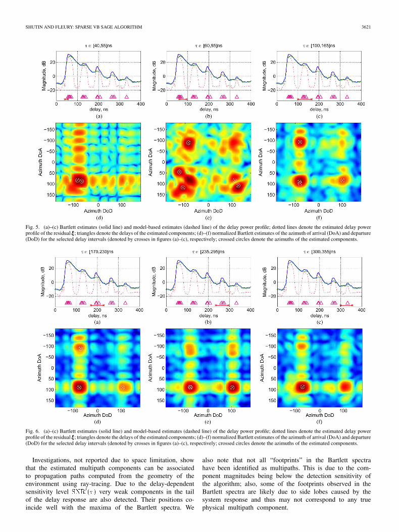
Fig. 5. (a)–(c) Bartlett estimates (solid line) and model-based estimates (dashed line) of the delay power profile; dotted lines denote the estimated delay powerprofile of the residual ��; triangles denote the delays of the estimated components; (d)–(f) normalized Bartlett estimates of the azimuth of arrival (DoA) and departure(DoD) for the selected delay intervals (denoted by crosses in figures (a)–(c), respectively; crossed circles denote the azimuths of the estimated components.

Fig. 6. (a)–(c) Bartlett estimates (solid line) and model-based estimates (dashed line) of the delay power profile; dotted lines denote the estimated delay powerprofile of the residual ��; triangles denote the delays of the estimated components; (d)–(f) normalized Bartlett estimates of the azimuth of arrival (DoA) and departure(DoD) for the selected delay intervals (denoted by crosses in figures (a)–(c), respectively; crossed circles denote the azimuths of the estimated components.

Investigations, not reported due to space limitation, showthat the estimated multipath components can be associatedto propagation paths computed from the geometry of theenvironment using ray-tracing. Due to the delay-dependentsensitivity level very weak components in the tailof the delay response are also detected. Their positions co-incide well with the maxima of the Bartlett spectra. We

also note that not all “footprints” in the Bartlett spectrahave been identified as multipaths. This is due to the com-ponent magnitudes being below the detection sensitivity ofthe algorithm; also, some of the footprints observed in theBartlett spectra are likely due to side lobes caused by thesystem response and thus may not correspond to any truephysical multipath component.


VII. CONCLUSION

This contribution proposes a new algorithm that estimatesthe number of relevant multipath components in the responseof radio channels and the parameters of these componentswithin the Bayesian framework. High-resolution estimation ofthe multipath components is performed using the VB-SAGEalgorithm—a new extension of the traditional SAGE algo-rithm—which allows for computing estimates of the posteriorpdfs of the component parameters, rather than parameter pointestimates. By introducing sparsity priors for the multipathcomponent gains, the sparse VB-SAGE algorithm estimatesthe posterior pdfs of the component parameters jointly withthe posterior pdfs of the sparsity parameters by minimizingthe variational free energy. The pdfs of the parameters of asingle component are updated at each iteration of the algorithm,with the iterations cycling through the components. Due to themonotonicity property of the VB-SAGE algorithm, the freeenergy is non-decreasing versus the iterations.

Several sparsity priors are considered: Gaussian, flat, andLaplace priors. The admissible hidden data introduced inthe VB-SAGE algorithm lead to simple and easy to interpretcomponent pruning rules/conditions for these priors. Thesesconditions are shown to be equivalent to removing signal com-ponents based on comparison of the per-component SNR witha given threshold. This threshold can be set for all componentsor tailored for each component individually.

The sparse VB-SAGE algorithm is applied to the estimationof the multipath components in the response of synthetic andmeasured wireless multipath channels. We show by means ofMonte Carlo simulations that the sparsity-based model orderselection methods with sensitivity-adjusted pruning conditionsoutperform the Bayesian Information Criterion and the neg-ative log-evidence model order selection criterion. The latterapproaches fail since, due to various effects (calibration errors,finite precision in the discretization process, diffuse scattering,etc.) leading to a model mismatch, numerical artifacts areintroduced, which lead to a decreasing RMSE at the expenseof an increased model order. In case of estimation of wirelesschannels this is highly undesirable, since the estimated artifactshave no physical meaning. The proposed modifications of thepruning conditions allow for correcting for possible modelorder estimation bias due to modeling mismatch. Making useof the Laplace prior results in the best performance amongthe tested methods. Simulations show that for low SNR theVB-SAGE algorithm with Laplace sparsity priors, which werefer to as the VB-SAGE-L algorithm, keeps only reliablyestimated components, while successfully removing the ar-tifacts. The VB-SAGE-L algorithm also exhibits the fastestconvergence as compared to the other tested algorithms withthe same stopping criterion.

We apply the VB-SAGE-L algorithm to the estimation of themultipath components in measured channel impulse responses.In order to minimize the effects of model mismatch, the detectorsensitivity is adjusted based on an estimate of the delaypower profile. Since the artifacts are typically more pronouncedin delay ranges associated with high received power, a smoothedversion of the delay power profile can be used as an indicator ofthe received power versus propagation delay. Investigations, notreported in this paper due to space limitation, show that the es-timated multipath components can be associated to propagation

paths computed from the geometry of the environment usingray-tracing.

The sparse VB-SAGE algorithm provides a new and effectivetool for efficient estimation of wireless channels. Its flexibilityand its iterative structure make it very attractive for many ap-plications in wireless communications: analysis and estimationof complex MIMO channel configurations in channel soundingand MIMO radars, channel estimation in iterative receivers per-forming joint channel estimation and data decoding, as well asextraction of location-dependent features of the radio channelfor localization purposes.

APPENDIX AMONOTONICITY PROPERTY OF THE VB-SAGE ALGORITHM

In what follows, we assume that the variational approx-imating pdf (6) and its factors are selected as outlined inSection III-A and is set to 1.

Define as the set of parameters associatedwith the th multipath component and

as the set of the other multipath parameters. We assumethat . It is straightforward to show thatminimizing the free energy with re-spect to is equivalent to minimizingwith . TheVB-SAGE algorithm facilitates this optimization using theadmissible hidden data in (3). Consider the equality

. By combiningthis equality with the factorization (4) and computing theexpectation with respect to and we obtain

where is a term independent of . Define now. Observe that is a func-

tion of the admissible hidden data and the th multipath compo-nent parameters. Now, the free energy with respect to can berewritten as

(31)

Minimizing is typically simpleras compared to minimizing .However, whether decreases as

decreases ultimately depends on the termin (31).

Let denote an existing (old) estimate of , andlet be the new minimizer of .A current estimate of the admissible hidden dataposterior pdf is given by (7), i.e.,

, since. Note that it is easy to show that

must be quadratic in . Similarly we define. With these set-

tings it follows that

(32)


Result (32) expresses the monotonicity property of theVB-SAGE algorithm. Furthermore,

is a sufficient con-dition that guarantees the monotonicity of the VB-SAGEalgorithm for our estimation problem.

REFERENCES

[1] T. S. Rappaport, Wireless Communications. Principles and Practice.Englewood Cliffs, NJ: Prentice-Hall PTR, 2002.

[2] H. Krim and M. Viberg, “Two decades of array signal processingresearch: The parametric approach,” IEEE Signal Process. Mag., pp.67–94, Jul. 1996.

[3] B. Fleury, M. Tschudin, R. Heddergott, D. Dahlhaus, and K. I. Ped-ersen, “Channel parameter estimation in mobile radio environmentsusing the SAGE algorithm,” IEEE J. Sel. Areas Commun., vol. 17, no.3, pp. 434–450, Mar. 1999.

[4] O. Besson and P. Stoica, “Decoupled estimation of DOA and angularspread for a spatially distributed source,” IEEE Trans. Signal Process.,vol. 48, no. 7, pp. 1872–1882, 2000.

[5] A. Richter, “Estimation of radio channel parameters: Models and algo-rithms,” Ph.D. dissertation, Tech. Univ. Ilmenau, Ilmenau, Germany,2005.

[6] H. Akaike, “A new look at the statistical model identification,” Trans.Autom. Control, vol. 19, no. 6, pp. 716–723, Dec. 1974.

[7] J. I. Myung, D. J. Navarro, and M. A. Pitt, “Model selection by nor-malized maximum likelihood,” J. Math. Psychol., vol. 50, pp. 167–179,2005.

[8] D. J. MacKay, Information Theory, Inference, and Learning Algo-rithms. Cambridge, U.K.: Cambridge Univ. Press, 2003.

[9] A. Lanterman, “Schwarz, Wallace, and Rissanen: Intertwining themesin theories of model order estimation,” Int. Statist. Rev., vol. 69, no. 2,pp. 185–212, 2000.

[10] M. Feder and E. Weinstein, “Parameter estimation of superimposedsignals using the EM algorithm,” IEEE Trans. Acoust., Speech, SignalProcess., vol. 36, no. 4, pp. 477–489, Apr. 1988.

[11] D. G. Tzikas, A. C. Likas, and N. P. Galatsanos, “The variational ap-proximation for Bayesian inference,” IEEE Signal Process. Mag., vol.25, no. 6, pp. 131–146, Nov. 2008.

[12] D. Malioutov, M. Cetin, and A. Willsky, “A sparse signal reconstruc-tion perspective for source localization with sensor arrays,” IEEETrans. Signal Process., vol. 53, no. 8, pp. 3010–3022, 2005.

[13] D. Wipf and B. Rao, “Sparse Bayesian learning for basis selection,”IEEE Trans. Signal Process. , vol. 52, no. 8, pp. 2153–2164, Aug. 2004.

[14] M. Tipping, “Sparse Bayesian learning and the relevance vector ma-chine,” J. Mach. Learn. Res., vol. 1, pp. 211–244, June 2001.

[15] M. Figueiredo, “Adaptive sparseness for supervised learning,” IEEETrans. Pattern Anal. Mach. Intell., vol. 25, no. 9, pp. 1150–1159, 2003.

[16] W. Bajwa, J. Haupt, A. Sayeed, and R. Nowak, “Compressed channelsensing: A new approach to estimating sparse multipath channels,”Proc. IEEE, vol. 98, no. 6, pp. 1058–1076, Jun. 2010.

[17] M. E. Tipping and A. C. Faul, “Fast marginal likelihood maximisationfor sparse Bayesian models,” in Proc. 9th Int. Workshop on Artif. Intell.Statist., Key West, FL, Jan. 2003.

[18] R. Neal, Bayesian Learning for Neural Networks, ser. Lecture Notes inStat.. New York: Springer-Verlag, 1996, vol. 118.

[19] D. Shutin, G. Kubin, and B. H. Fleury, “Application of the evidenceprocedure to the analysis of wireless channels,” EURASIP J. Adv.Signal Process., vol. 2007, pp. 1–23, 2007.

[20] Y. Tsaig and D. L. Donoho, “Extensions of compressed sensing,”Signal Process., vol. 86, no. 3, pp. 549–571, 2006.

[21] J. W. Wallace and M. A. Jensen, “Sparse power angle spectrum esti-mation,” IEEE Trans. Antennas Propag., vol. 57, no. 8, pp. 2452–2460,Aug. 2009.

[22] P. Zhao and B. Yu, “On model selection consistency of LASSO,” J.Mach. Learn. Res., vol. 7, pp. 2541–2563, 2006.

[23] D. L. Donoho and M. Elad, “Optimally sparse representation in general(nonorthogonal) dictionaries via � minimization,” Proc. Nat. Acad. ofSci. USA, vol. 100, no. 5, pp. 2197–2202, 2003.

[24] R. Tibshirani, “Regression shrinkage and selection via the LASSO,” J.R. Statist. Soc., vol. 58, pp. 267–288, 1994.

[25] M. Figueiredo, R. Nowak, and S. Wright, “Gradient projection forsparse reconstruction: Application to compressed sensing and otherinverse problems,” IEEE J. Sel. Topics Signal Process. , vol. 1, no. 4,pp. 586–597, Dec. 2007.

[26] Y. Chi, A. Pezeshki, L. Scharf, and R. Calderbank, “Sensitivity to basismismatch in compressed sensing,” in Proc. Int. Conf. Acoust., Speech,Signal Process. , 2010.

[27] M. J. Beal, “Variational algorithm for approximate Bayesian infer-ence,” Ph.D. dissertation, Univ. College London, London, U.K., 2003.

[28] J. Fessler and A. Hero, “Space-alternating generalized expectation-maximization algorithm,” IEEE Trans. Signal Process., vol. 42, pp.2664–2677, Oct. 1994.

[29] D. Shutin and H. Koeppl, “Application of the evidence procedure tolinear problems in signal processing,” in Proc. 24th Int. Workshopon Bayesian Infer. Max. Entr. Methods in Sci. Eng., Jul. 2004, pp.124–127.

[30] D. J. C. MacKay, “Bayesian methods for backpropagation networks,”in Models of Neural Networks III, E. Domany, J. L. van Hemmen,and K. Schulten, Eds. New York: Springer-Verlag, 1994, ch. 6, pp.211–254.

[31] C. M. Bishop, Pattern Recognition and Machine Learning (InformationScience and Statistics). : Springer, Aug. 2006.

[32] J. Salmi, A. Richter, and V. Koivunen, “Detection and tracking ofMIMO propagation path parameters using state-space approach,”IEEE Trans. Signal Process., vol. 57, no. 4, pp. 1538–1550, Apr. 2009.

[33] H. L. V. Trees, Optimum Array Processing: Part IV of Detection, Esti-mation, and Modulation Theory. New York: Wiley, 2002.

[34] N. Czink, E. Bonek, L. Hentila, J.-P. Nuutinen, and J. Ylitalo,“Cluster-based MIMO channel model parameters extracted fromindoor time-variant measurements,” in Proc. Global Telecommun.Conf. (GLOBECOM ’06), Nov. 27, 2006.

Dmitriy Shutin (S’02–M’06) received theMaster’s degree in computer science in 2000from Dniepropetrovsk State University, Ukraine, andthe Ph.D. degree in electrical engineering from GrazUniversity of Technology, Graz, Austria, in 2006.

During 2001–2006 and 2006–2009, he was aTeaching Assistant and an Assistant Professor,respectively, with the Signal Processing and SpeechCommunication Laboratory, Graz University ofTechnology. Since 2009, he has been a ResearchAssociate with the Department of Electrical Engi-

neering, Princeton University, Princeton, NJ. His current research interestsinclude stochastic modeling and estimation of the radio channel for MIMOapplications, distributed inference techniques in agent/sensor networks, radarsignal processing, and statistical pattern recognition.

Dr. Shutin was a recipient of the Best Student Paper Award at the 2005IEEE International Conference on Information, Communications and SignalProcessing (ICICS). In 2009 he was awarded the Erwin Schrödinger ResearchFellowship.

Bernard H. Fleury (M’97–SM’99) received theDiploma in electrical engineering and mathematicsin 1978 and 1990, respectively, and the Ph.D. degreein electrical engineering from the Swiss FederalInstitute of Technology Zurich (ETHZ) in 1990.

Since 1997, he has been with the Department ofElectronic Systems, Aalborg University, Denmark,as a Professor of communication theory. He is theHead of the Section Navigation and Communi-cations, which is one of the eight laboratories ofthis Department. From 2006 to 2009, he was a

Key Researcher with Telecommunications Research Center Vienna (FTW),Austria. During 1978–1985 and 1992–1996, he was a Teaching Assistantand a Senior Research Associate, respectively, with the CommunicationTechnology Laboratory, ETHZ. Between 1988 and 1992, he was a ResearchAssistant with the Statistical Seminar at ETHZ. His research interests covernumerous aspects within communication theory and signal processing, mainlyfor wireless communications. His current activities include stochastic modelingand estimation of the radio channel especially for MIMO applications in fasttime-varying environments, iterative message-passing processing with focus onthe design of efficient feasible architectures for wireless receivers, localizationtechniques in wireless terrestrial systems, and radar signal processing. He hasauthored and coauthored more than 110 publications in these areas. He hasdeveloped, with his staff, a high-resolution method for the estimation of radiochannel parameters that has found a wide application and has inspired similarestimation techniques both in academia and in industry.

Aalborg Universitet Sparse Variational Bayesian SAGE...

Documents

Transcript of Aalborg Universitet Sparse Variational Bayesian SAGE...