Aalborg Universitet Learning with Hidden Variables ... · I would like to thank a number of people...
124
Aalborg Universitet Learning with Hidden Variables Karciauskas, Gytis Publication date: 2005 Document Version Publisher's PDF, also known as Version of record Link to publication from Aalborg University Citation for published version (APA): Karciauskas, G. (2005). Learning with Hidden Variables: A Parameter Reusing Approach for Tree-Structured Bayesian Networks. Department of Computer Science, Aalborg University. General rights Copyright and moral rights for the publications made accessible in the public portal are retained by the authors and/or other copyright owners and it is a condition of accessing publications that users recognise and abide by the legal requirements associated with these rights. ? Users may download and print one copy of any publication from the public portal for the purpose of private study or research. ? You may not further distribute the material or use it for any profit-making activity or commercial gain ? You may freely distribute the URL identifying the publication in the public portal ? Take down policy If you believe that this document breaches copyright please contact us at [email protected] providing details, and we will remove access to the work immediately and investigate your claim. Downloaded from vbn.aau.dk on: April 26, 2017
-
Upload
vuongkhanh -
Category
Documents
-
view
212 -
download
0
Transcript of Aalborg Universitet Learning with Hidden Variables ... · I would like to thank a number of people...

Aalborg Universitet
Learning with Hidden Variables
Karciauskas, Gytis
Publication date:2005
Document VersionPublisher's PDF, also known as Version of record
Link to publication from Aalborg University
Citation for published version (APA):Karciauskas, G. (2005). Learning with Hidden Variables: A Parameter Reusing Approach for Tree-StructuredBayesian Networks. Department of Computer Science, Aalborg University.
General rightsCopyright and moral rights for the publications made accessible in the public portal are retained by the authors and/or other copyright ownersand it is a condition of accessing publications that users recognise and abide by the legal requirements associated with these rights.
? Users may download and print one copy of any publication from the public portal for the purpose of private study or research. ? You may not further distribute the material or use it for any profit-making activity or commercial gain ? You may freely distribute the URL identifying the publication in the public portal ?
Take down policyIf you believe that this document breaches copyright please contact us at [email protected] providing details, and we will remove access tothe work immediately and investigate your claim.
Downloaded from vbn.aau.dk on: April 26, 2017

Learning with Hidden Variables:A Parameter Reusing Approach forTree-Structured Bayesian Networks
Gytis KarciauskasDepartment of Computer Science
Aalborg University
Ph.D. Thesis
2005

Læring af skjulte variable:Genbrug af parametre for
træstrukturerede Bayesianske net
(title in Danish)
i

Summary
In this thesis we address the problem of learning the cardinalities of hiddenvariables and model parameters in tree-structured Bayesian networks withhidden variables. We work with latent class (LC) models and hierarchical la-tent class (HLC) models, which are among the simplest types of Bayesian net-works with hidden variables for categorical data. The standard approachesfor learning cardinalities and parameters in Bayesian networks with hiddenvariables often find only local maximum solutions or are too expensive com-putationally. We propose the so-called parameter reusing approach that usesparameters from a previously learned model for determining parameters of anext model. Modified parameters of the previous model are used as a start-ing configuration for the EM algorithm, which optimises the parameters ofthe next model. We reuse the parameters by splitting or merging compo-nents (i.e., states of a hidden variable). We discuss theoretical properties ofsuch operations in the context of LC models. We propose algorithms thatlearn cardinalities and parameters in LC and HLC models by performingcomponent splitting, merging, and an operation that combines these two. Inexperiments with synthetic and real data, these algorithms in a majority ofcases performed better than the algorithms that use standard starting con-figurations for EM. In particular, the parameter reusing approach was betterfor bigger-sized training data. At the end, we propose some improvementsof our algorithms and discuss how the parameter reusing approach could beextended to unrestricted Bayesian networks with hidden variables.
ii

Acknowledgements
I would like to thank a number of people who helped me in this Ph.D. project.First, I would like to thank my supervisor Finn V. Jensen for all his guidanceand support. Also I thank Tomas Kocka for all the discussions, ideas, and forthose days in Prague. I thank Nevin L. Zhang for his help concerning HLCmodels and especially for his source code. Also I thank Pedro Larranagaand Jose A. Lozano for the support during my stay at the University ofthe Basque Country. And of course thanks to all the people I met in theMachine Intelligence (or the Decision Support Systems) group in Aalborg,in the Intelligent Systems Group in San Sebastian, and in the Institute ofInformation Theory and Automation in Prague.
iii

Contents
1 Introduction 1
2 Notation and Definitions 3
3 Related Work 73.1 Learning the Structure with Hidden Variables . . . . . . . . . 7
3.1.1 Detecting Hidden Variables . . . . . . . . . . . . . . . 83.1.2 Learning the Cardinalities . . . . . . . . . . . . . . . . 103.1.3 Scoring the Structures . . . . . . . . . . . . . . . . . . 10
3.2 Estimating the Parameters . . . . . . . . . . . . . . . . . . . . 123.3 Parameter Reusing . . . . . . . . . . . . . . . . . . . . . . . . 143.4 LC and HLC Models . . . . . . . . . . . . . . . . . . . . . . . 16
3.4.1 Latent Class Models . . . . . . . . . . . . . . . . . . . 163.4.2 Hierarchical Latent Class Models . . . . . . . . . . . . 17
4 Increasing the Cardinality 214.1 Overview . . . . . . . . . . . . . . . . . . . . . . . . . . . . . . 214.2 Definitions . . . . . . . . . . . . . . . . . . . . . . . . . . . . . 224.3 Theoretical Properties . . . . . . . . . . . . . . . . . . . . . . 23
4.3.1 Component Introduction . . . . . . . . . . . . . . . . . 234.3.2 Component Splitting . . . . . . . . . . . . . . . . . . . 254.3.3 Implications for Model Selection . . . . . . . . . . . . . 33
4.4 Implementation . . . . . . . . . . . . . . . . . . . . . . . . . . 334.4.1 Component Introduction vs. Component Splitting . . . 334.4.2 Component Splitting in Detail . . . . . . . . . . . . . . 38
4.5 Experiments . . . . . . . . . . . . . . . . . . . . . . . . . . . . 404.5.1 Algorithms . . . . . . . . . . . . . . . . . . . . . . . . 404.5.2 Setup of Experiments . . . . . . . . . . . . . . . . . . . 424.5.3 Results . . . . . . . . . . . . . . . . . . . . . . . . . . . 434.5.4 Discussion . . . . . . . . . . . . . . . . . . . . . . . . . 47
iv

CONTENTS
5 Decreasing the Cardinality 495.1 Overview . . . . . . . . . . . . . . . . . . . . . . . . . . . . . . 495.2 Definitions . . . . . . . . . . . . . . . . . . . . . . . . . . . . . 505.3 Theoretical Properties . . . . . . . . . . . . . . . . . . . . . . 51
5.3.1 Identifiability . . . . . . . . . . . . . . . . . . . . . . . 515.3.2 Component Merging for Identifiable Structures . . . . . 525.3.3 Component Merging when Variables are Binary . . . . 535.3.4 Summary . . . . . . . . . . . . . . . . . . . . . . . . . 54
5.4 Implementation . . . . . . . . . . . . . . . . . . . . . . . . . . 55
6 Learning of Latent Class Models 566.1 Parameter Adjustment . . . . . . . . . . . . . . . . . . . . . . 566.2 Algorithms . . . . . . . . . . . . . . . . . . . . . . . . . . . . . 58
6.2.1 Algorithm Based on Splitting and Merging . . . . . . . 586.2.2 Algorithms Based on Standard Starting Points . . . . . 62
6.3 Experiments . . . . . . . . . . . . . . . . . . . . . . . . . . . . 636.3.1 Setup of Experiments . . . . . . . . . . . . . . . . . . . 636.3.2 Results for Synthetic Data . . . . . . . . . . . . . . . . 646.3.3 Results for Real Data . . . . . . . . . . . . . . . . . . . 716.3.4 Discussion . . . . . . . . . . . . . . . . . . . . . . . . . 77
7 Learning of Hierarchical Latent Class Models 817.1 Parameter Reusing for HLC Models . . . . . . . . . . . . . . . 817.2 Algorithms . . . . . . . . . . . . . . . . . . . . . . . . . . . . . 82
7.2.1 Algorithm Based on Splitting and Merging . . . . . . . 827.2.2 Algorithms Based on Standard Starting Points . . . . . 87
7.3 Experiments . . . . . . . . . . . . . . . . . . . . . . . . . . . . 897.3.1 Setup of Experiments . . . . . . . . . . . . . . . . . . . 897.3.2 Results for Synthetic Data . . . . . . . . . . . . . . . . 907.3.3 Results for Real Data . . . . . . . . . . . . . . . . . . . 957.3.4 Discussion . . . . . . . . . . . . . . . . . . . . . . . . . 98
8 Conclusions and Research Directions 100
A Preprocessing of Text Data 103
Bibliography 105
Index 113
v

List of Tables
4.1 An example of P (X1, X2, X3) distribution. . . . . . . . . . . . 274.2 Results for Standard and Splitting. . . . . . . . . . . . . . . . . 444.3 Results for StandardFixed and Splitting. . . . . . . . . . . . . . 44
5.1 Results of experiments about properties of component merging. 54
6.1 Sampled from a 3:3x3 model. . . . . . . . . . . . . . . . . . . 656.2 Sampled from a 10:7x2 model. . . . . . . . . . . . . . . . . . . 656.3 Sampled from a 10:10x2 model. . . . . . . . . . . . . . . . . . 656.4 Sampled from a 10:15x2 model. . . . . . . . . . . . . . . . . . 666.5 Sampled from a 10:10x3 model. . . . . . . . . . . . . . . . . . 666.6 Sampled from a 5:20x2 model. . . . . . . . . . . . . . . . . . . 666.7 Sampled from the 10:15x2 model, no time limit. . . . . . . . . 666.8 Sampled from models having different structures. . . . . . . . 676.9 Sampled from 10:10x2 models, |D| = 106. . . . . . . . . . . . . 676.10 Sampled from 10:10x3 models, |D| = 104. . . . . . . . . . . . . 686.11 Sampled from m:10x2 models. . . . . . . . . . . . . . . . . . . 686.12 Description of real data sets. . . . . . . . . . . . . . . . . . . . 726.13 Results for real data. . . . . . . . . . . . . . . . . . . . . . . . 736.14 Results for “Spambase” data set, no time limit. . . . . . . . . 736.15 Results for real data: SplitMerge without parameter adjustment. 746.16 A summary of the results for synthetic data. . . . . . . . . . . 78
7.1 Sampled from the first model with 7 observed variables. . . . . 917.2 Sampled from the second model with 7 observed variables. . . 917.3 Sampled from models with 12 and with 18 observed variables. 927.4 Results for CoIL data set. . . . . . . . . . . . . . . . . . . . . 95
vi

List of Figures
3.1 A latent class model. . . . . . . . . . . . . . . . . . . . . . . . 163.2 An example of a hierarchical latent class model. . . . . . . . . 183.3 A model obtained by root walking. . . . . . . . . . . . . . . . 19
4.1 Two-dimensional continuous training data. . . . . . . . . . . . 344.2 The two–component model for the training data. . . . . . . . 354.3 The three–component model for the training data. . . . . . . . 354.4 Splitting of a component. . . . . . . . . . . . . . . . . . . . . . 364.5 Another two-dimensional continuous training data. . . . . . . 364.6 The two–component model for the training data. . . . . . . . 364.7 The three–component model for the training data. . . . . . . . 374.8 Score change during time for Corn10 data set. . . . . . . . . . 454.9 Score change during time for Mushroom data set. . . . . . . . 46
6.1 Score change during time for data sampled from the 10:10x2model, |D| = 106. . . . . . . . . . . . . . . . . . . . . . . . . . 69
6.2 Score change during time for data sampled from the 10:15x2model, |D| = 106. . . . . . . . . . . . . . . . . . . . . . . . . . 69
6.3 Score change during time for data sampled from the 10:7x3model, |D| = 106. . . . . . . . . . . . . . . . . . . . . . . . . . 70
6.4 Score change during time for “Mushroom” data set. . . . . . . 746.5 Score change during time for “Thyroid” data set. . . . . . . . 756.6 Score change during time for “Image” data set. . . . . . . . . 756.7 Score change during time for “Voting” data set. . . . . . . . . 76
7.1 Structure with 7 observed variables. . . . . . . . . . . . . . . . 907.2 Structure with 12 observed variables. . . . . . . . . . . . . . . 917.3 Structure with 18 observed variables. . . . . . . . . . . . . . . 927.4 Score change during time for data sampled from the first model
with 7 observed variables, |D| = 106. . . . . . . . . . . . . . . 92
vii

LIST OF FIGURES
7.5 Score change during time for data sampled from the secondmodel with 7 observed variables, |D| = 104. . . . . . . . . . . 93
7.6 Score change during time for data sampled from the secondmodel with 7 observed variables, |D| = 106. . . . . . . . . . . 93
7.7 Score change during time for data sampled from the modelwith 12 observed variables. . . . . . . . . . . . . . . . . . . . . 94
7.8 Score change during time for data sampled from the modelwith 18 observed variables. . . . . . . . . . . . . . . . . . . . . 94
7.9 HLC model structure for CoIL data set. . . . . . . . . . . . . 967.10 Score change during time for CoIL data set. . . . . . . . . . . 97
viii

List of Procedures
4.1 Splitting(D) . . . . . . . . . . . . . . . . . . . . . . . . . . . . 414.2 Standard(D) . . . . . . . . . . . . . . . . . . . . . . . . . . . . 414.3 StandardFixed(D,m) . . . . . . . . . . . . . . . . . . . . . . . 426.1 SplitMerge(D) . . . . . . . . . . . . . . . . . . . . . . . . . . . 596.2 Split(L,D) . . . . . . . . . . . . . . . . . . . . . . . . . . . . . 606.3 Merge(L,D) . . . . . . . . . . . . . . . . . . . . . . . . . . . . 616.4 Adjust(L,D) . . . . . . . . . . . . . . . . . . . . . . . . . . . 627.1 HLCSplitMerge(D, s) . . . . . . . . . . . . . . . . . . . . . . . 847.2 HLCSplit(L,D) . . . . . . . . . . . . . . . . . . . . . . . . . . 857.3 HLCMerge(L,D) . . . . . . . . . . . . . . . . . . . . . . . . . 857.4 HLCAdjust(L,D) . . . . . . . . . . . . . . . . . . . . . . . . . 867.5 HLCIncrement(L,D) . . . . . . . . . . . . . . . . . . . . . . . 877.6 HLCDecrement(L,D) . . . . . . . . . . . . . . . . . . . . . . . 887.7 HLCNewParams(L,D) . . . . . . . . . . . . . . . . . . . . . . 887.8 HLCStandardFixed(D,m) . . . . . . . . . . . . . . . . . . . . 89
ix

Chapter 1
Introduction
Bayesian networks (Pearl, 1988), also known as probabilistic networks orBayesian belief networks, allow a representation of joint probability distri-butions in a compact way and have become popular in the field of ArtificialIntelligence. As construction of Bayesian networks by using human expertknowledge is often a hard process, recently lots of research has been doneon automatic learning of Bayesian networks from data (Neapolitan, 2003).For complete data (i.e., data where each variable from a Bayesian network isalways observed), many algorithms have been proposed and strong theoret-ical results have been obtained (Chickering, 2002). For Bayesian networkswith hidden variables (i.e., variables that are never observed in given data),the problem of learning a network from data becomes more challenging andthe available algorithms provide only partial solutions. When learning withhidden variables, the problems of determining the number and cardinalitiesof hidden variables appear in addition to the usual problems of determininglinks between variables and model parameters. And even the problem of de-termining model parameters alone is much more difficult than in the case ofcomplete data.
In this thesis, we address the problem of determining the cardinalities ofhidden variables and model parameters assuming a fixed number of hiddenvariables and fixed links between variables in a model. The standard ap-proaches for determining cardinalities and parameters often find only localmaximum solutions or are too expensive computationally. We propose theso-called parameter reusing approach that uses parameters from a previouslylearned model for determining parameters of a next model. This often al-lows to find better solutions in the same time. We work with tree-structuredBayesian networks: latent class (LC) (Lazarsfeld and Henry, 1968; Good-man, 1974) and hierarchical latent class (HLC) (Zhang, 2004) models. Theyare among the simplest types of Bayesian networks with hidden variables for
1

Introduction
categorical data. A nice feature of tree-structured Bayesian networks is thatinference there is faster than in unrestricted Bayesian networks, because eachvariable can have no more than one parent.
This thesis is organised as follows. In next chapter we introduce the no-tation and definitions that will be used throughout the thesis. In Chapter 3we overview the related work on learning with hidden variables. There wediscuss learning of Bayesian networks with hidden variables, overview therelated work on parameter reusing, and give an introduction to LC and HLCmodels. In Chapter 4 we discuss approaches for increasing the cardinalityof a hidden variable while reusing the parameters in LC models. We provethe theoretical properties of the proposed approaches, discuss the implemen-tation, and present the experiments performed. In Chapter 5 we discussapproaches for decreasing the cardinality of a hidden variable while reusingthe parameters in LC models. We discuss the theoretical properties of theproposed approaches and the implementation. In Chapter 6 we discuss learn-ing of LC models by combining the operations introduced in Chapters 4 and5. We describe the algorithms for learning LC models and present the exper-iments performed. In Chapter 7 we extend our parameter reusing approachto HLC models. We describe the algorithms for learning HLC models andpresent the experiments performed. In Chapter 8 we conclude this thesis anddiscuss possible directions for further research.
2

Chapter 2
Notation and Definitions
In this chapter we give notation and definitions which will be used in thisthesis.
A categorical or continuous variable is denoted by an upper-case letter(for example, Di), a state of a variable by a lower-case letter (for example,di). A vector of states for a set of variables is denoted by a bold lower-case letter (for example, d). Data (or data set) over variables D1, . . . , Dk
is D = (〈d1, n1〉, . . . , 〈dN , nN〉), where each instance dj is a k-dimensionalvector, instance weight nj ≥ 0 is a real number, and dj 6= dj′ for j 6= j′.1
The size of data D is |D| = ∑Nj=1 nj.
If a value of some Di is not observed in some dj, we say that dj containsmissing data. If there exists such dj, we say that D contains missing data.Otherwise, D is called complete.
For a categorical variable X, |X| denotes the cardinality (the number ofpossible states) and dom(X) denotes the domain (the set of possible states)of X.
P denotes a probability distribution when it has variables as arguments.Otherwise, it denotes a single probability. PD(D1, . . . , Dk) denotes the jointprobability distribution obtained from D.2 That is,
PD(d) =
{ nj
|D| if d = dj for some 1 ≤ j ≤ N
0 otherwise(2.1)
The Kulbach-Leibler distance between probability distributions
1Please note that we do not require weights nj to be integers, but allow them to bereal numbers. This will simplify a notation in some places.
2Here we assume that D over D1, . . . , Dk is complete.
3

Notation and Definitions
P1(D1, . . . , Dk) and P2(D1, . . . , Dk) is
KL(P1, P2) =∑
d∈D1×...×Dk
P2(d) logP2(d)
P1(d)(2.2)
A model is denoted by an upper-case letter (for example, M) and is usedfor representing a joint probability distribution PM(D1, . . . , Dk). Model Mis specified by its structure m and parameters θ. That is, M = (m, θ). Themarginal likelihood of data D given model structure m is
P (D|m) =
∫P (D|θ,m) P (θ|m) dθ (2.3)
P (D|θ,m) = P (D|M) is called the likelihood of D given M .
P (D|M) =N∏
j=1
PM(dj)nj (2.4)
where PM(d) is the probability of d given M . The log-likelihood of D givenM is denoted as
LL(D|M) = ln P (D|M) =N∑
j=1
nj ln PM(dj) (2.5)
We say that D is described perfectly by model M if PM(D1, . . . , Dk) =PD(D1, . . . , Dk).
For fixed D and m, the maximum a posteriori (MAP) parameters are
θMAP = arg maxθ
P (θ|D,m) = arg maxθ
P (D|θ,m) P (θ|m)
P (D|m)
= arg maxθ
P (D|θ,m) P (θ|m) (2.6)
and the maximum likelihood (ML) parameters are
θML = arg maxθ
P (D|θ,m) (2.7)
For a model M , dim(M) denotes the number of independent parametersin M (that is, the standard dimension of M). For a model structure m,dim(m) is equal to dim(M) of any model M having structure m.
A variable from M that is never observed in D is called a hidden variable.Otherwise, it is called an observed variable. So, if M contains a hidden
4

Notation and Definitions
variable, D over all the variables from M automatically contains missingdata.
When using the term structure for models with hidden variables, we as-sume that cardinalities of hidden variables are also specified in a structure.We use the term skeleton for what is left when information about cardinali-ties of hidden variables is removed from a structure. So, structure m = (s, c),where s is a skeleton of a model and c specifies cardinalities of hidden vari-ables.
M is a mixture of m models if
PM(d) =m∑
l=1
PM(hl) PM(d|hl) (2.8)
where PM(hl) is the weight of the lth model, PM(d|hl) depends only onparameters of the lth model, and
∑ml=1 PM(hl) = 1. So, a mixture can be
seen as a model containing hidden variable H with states h1, . . . , hm, whereeach state corresponds to one of m models. For mixtures, we will also use theterm component to indicate one of m models (i.e., one of states h1, . . . , hm).
Dl denotes the part of D that probabilistically belongs to component hl
in a mixture model. Formally,
Dl = (〈d1, nl1〉, . . . , 〈dN , nlN〉) (2.9)
where nlj = njPM(hl|dj) (so,∑m
l=1 nlj = nj,∀j = 1, . . . , N). Here
PM(hl|dj) =PM(hl)PM(dj|hl)
PM(dj)(2.10)
A mixture model M is a Gaussian mixture if each PM(d|hl) is a k-dimensional Gaussian distribution. That is,
PM(d|hl) = (2π)−k2 |Cl|− 1
2 exp
(−1
2(d−ml)
TC−1l (d−ml)
)(2.11)
where mean vector ml and covariance matrix Cl constitute the parametersof component hl.
Model M = (m, θ) is a Bayesian network with variables X1, . . . , Xn if (1)structure m corresponds to a directed acyclic graph with nodes X1, . . . , Xn
3
and (2) parameters θ consist of probability distributions PM(Xi|pa(Xi)), i =1, . . . , n, where pa(X) is a set of parents of X in m. Then
PM(X1, . . . , Xn) =n∏
i=1
PM(Xi|pa(Xi)) (2.12)
3We use the terms node and variable interchangeably.
5

Notation and Definitions
In this thesis, we consider only Bayesian networks with categorical variables.xv
i denotes the vth state of variable Xi and paui denotes the uth configuration
of parents of Xi. qi denotes the number of possible configurations of parentsof Xi (i.e., qi =
∏Y ∈pa(Xi)
|Y |).Note that for a Bayesian network M
dim(M) =n∑
i=1
(|Xi| − 1) qi (2.13)
6

Chapter 3
Related Work
In this chapter we overview the related work on learning with hidden vari-ables. First, we discuss learning the structure of Bayesian networks withhidden variables, then estimating their parameters. Then we overview therelated work on parameter reusing. Finally, we give an introduction to latentclass and hierarchical latent class models.
3.1 Learning the Structure with Hidden
Variables
Much research has been done on learning Bayesian network structure fromcomplete data (Heckerman, 1995), and strong theoretical results have beenobtained for tree-structured networks in particular (Chow and Liu, 1968) andfor unrestricted networks in general (Chickering, 2002). When learning fromcomplete data D, it is not difficult to evaluate a Bayesian network structurem, because the marginal likelihood P (D|m) has a closed-form solution:
P (D|m) =n∏
i=1
qi∏u=1
Γ(αiu)
Γ(αiu + Niu)·|Xi|∏v=1
Γ(αiuv + Niuv)
Γ(αiuv)(3.1)
where Niuv is the sum of weights of instances where Xi is in state xvi and
pa(Xi) are in configuration paui (i.e., Niuv =
∑j: Xi=xv
i ,pa(Xi)=paui in dj
nj),
αiuv is the corresponding parameter of the Dirichlet prior, Niu =∑|Xi|
v=1 Niuv,
and αiu =∑|Xi|
v=1 αiuv.The problem of learning Bayesian network structure becomes more chal-
lenging when some data is missing, especially when there are hidden vari-ables. As shown by Cooper and Herskovits (1992) and Cooper (1995), in
7

Related Work 3.1. Learning the Structure with Hidden Variables
theory one could consider all the possible assignments of hidden variablestates to the instances in the data set and then use Formula 3.1 for com-plete data to evaluate a Bayesian network structure. However, in practice toconsider all the possible assignments of hidden variable states is extremelyexpensive computationally.
Probably the best known practical contribution is the Structural EM algo-rithm (Friedman, 1997; Friedman, 1998), where the EM algorithm (describedin Section 3.2) is extended to learning structures with hidden variables. Themain idea is to complete data as in the E-step of the standard EM, and thento use the completed data to evaluate adjustments of a structure. These twosteps are repeated iteratively. The algorithm has been proved to convergeand experiments show good performance. The disadvantage is that the num-ber of hidden variables and the cardinality of each hidden variable must befixed.
3.1.1 Detecting Hidden Variables
The problem of automatically detecting hidden variables has been addressedby many researchers.
Pearl (1986) proposes an algorithm for learning tree-structured Bayesiannetworks where non-leafs are hidden variables. All the variables are assumedto be binary. The network structure is learned by computing correlations forpairs of observed variables. The algorithm is fast and it discovers the trueBayesian network. However, it assumes that the observed variables can bedescribed by such a tree-structured network and that precise correlation coef-ficients are known. Liu et al. (1990) extend the algorithm of Pearl (1986) byallowing errors in correlation data occur. Their algorithm performs greedysearch for network structure. This algorithm does not have theoretical guar-antees any longer, but is applicable to real data.
The FCI algorithm of Spirtes et al. (1993); Spirtes et al. (2000) learnsthe Bayesian network structure by performing multiple tests of conditionalindependence. Under some assumptions, the algorithm sometimes indicatesthe existence of a hidden common cause for observed variables. However, thealgorithm does not perform well on data of small size.
The algorithm of Connolly (1993) learns tree-structured Bayesian net-works where non-leafs are hidden variables. Differently from Pearl (1986)and Liu et al. (1990), the variables are not required to be binary. Observedvariables are grouped by computing mutual information. The cardinalitiesof hidden variables are determined by conceptual clustering (Fisher, 1987).
The algorithm of Martin and VanLehn (1995) learns Bayesian networksthat contain edges only from hidden variables to observed ones. The al-
8

Related Work 3.1. Learning the Structure with Hidden Variables
gorithm computes correlation for each pair of observed variables and thenintroduces hidden variables to explain dependencies between observed ones.To determine the cardinalities of hidden variables and model parameters,the algorithm uses a fast approximation of the normative approach ofCooper and Herskovits (1992); Cooper (1995). Instead of considering assign-ments of hidden variable states for all the instances in the data set at once,it considers these assignments for one instance at a time. In the beginning,the cardinality of each hidden variable is set to 1. Then the algorithm goesthrough all the instances, one at a time. For the jth instance, it finds themost probable state of each hidden variable (or introduces the new state of ahidden variable, if this is the best for describing the jth instance) given thecurrent model, which is based on previous j−1 instances. Then the algorithmupdates model parameters according to these most probable assignments ofhidden variable states.
Kwoh and Gillies (1996) propose an algorithm that creates a hidden nodewhen the observed variables having the same parent are not conditionally in-dependent. The hidden node is then introduced between those variables andtheir parent. The algorithm searches for conditional dependencies by com-puting conditional correlation and/or mutual information between observedvariables in the already available network.
Ramachandran and Mooney (1998) propose an algorithm that can addhidden nodes in order to improve a classification accuracy of Bayesian net-work classifiers with noisy-or and noisy-and nodes. For Dynamic Bayesiannetworks, Boyen et al. (1999) introduce hidden variables by searching for vi-olations of the Markov property.
Elidan et al. (2000) propose a heuristic for detecting hidden variables inBayesian networks. First, a network over the observed variables is learned.Next, a search for “structural signatures” of hidden variables in the learnednetwork is performed. The algorithm searches for semi-cliques – sets of vari-ables where each variable is linked to at least half of the variables in that set.Candidate hidden variables are introduced as parents of variables in semi-cliques. Finally, each candidate is evaluated and the best scoring network isselected.
Tian and Pearl (2002) propose a systematic procedure of identifyingfunctional constraints induced by Bayesian networks with hidden variables.Their procedure can be used for inferring structures with hidden variablesfrom data.
9

Related Work 3.1. Learning the Structure with Hidden Variables
3.1.2 Learning the Cardinalities
The simplest and probably the most popular approach for learning the car-dinality of a hidden variable is to learn independently a different model fordifferent cardinalities of a hidden variable and then select the best model(Chickering and Heckerman, 1997; Uebersax, 2001; NorsysSoftwareCorp.,2005). However, this requires a separate estimation of parameters for eachmodel, which can be very time consuming.
The algorithms of Connolly (1993) and Martin and VanLehn (1995), de-scribed in the previous section, try to determine the cardinalities of hiddenvariables.
Another fast heuristic approach has been proposed byElidan and Friedman (2001). For each instance from training data, anassignment to a particular state of a hidden variable is maintained. Becauseof this, complete data scoring function can be used. The algorithm startswith a maximal possible number of states of a hidden variable and mergesstates pairwise in a greedy way until all the states are merged into one state.Two states are merged into a new one by assigning to the new state allthe instances that have previously been assigned to one of these two states.When merging in a greedy way, the algorithm selects to merge such twostates that the resulting model has the highest complete data score. Aftera separate model for each cardinality has been obtained, the algorithmselects the cardinality that corresponds to the highest scoring model. Thecardinalities of two or more interacting hidden variables are learned byrepeatedly selecting one variable and learning its cardinality while keepingthe cardinalities of other variables fixed.
3.1.3 Scoring the Structures
When selecting among structures of Bayesian networks with hidden vari-ables, some problems with scoring methods also appear. For missing data, theclosed-form solution (Formula 3.1) for determining the marginal likelihood ofcomplete data can no longer be used. As Chickering and Heckerman (1997)point out, one must use large sample approximations (such as Laplace, BIC,Cheeseman-Stutz scores) or Monte-Carlo approaches, which are more ac-curate but also more expensive computationally. When computing a largesample approximation for a structure m, ML or MAP parameters θ′ for mhave to be computed. That is why we will also say that a large sampleapproximation evaluates a parameterised model M = (m, θ), where θ is anestimate of θ′.
10

Related Work 3.1. Learning the Structure with Hidden Variables
Mostly we will use a well-known BIC score (Schwarz, 1978), defined as
BIC (M) = LL(D|M)− dim(M)
2ln |D| (3.2)
Assuming that the parameters of model M are those of maximum likelihood,BIC score is asymptotically correct for Bayesian networks without hiddenvariables (Schwarz, 1978; Haughton, 1988; Geiger et al., 2001).
Sometimes we will use Cheeseman-Stutz (CS) score (Cheeseman andStutz, 1995), defined as
CS (M) = LL(D|M)− LL(D′|M) + log P (D′|m) (3.3)
where m is the structure of model M and D′ is obtained by com-pleting D using model M . Here P (D′|m) has a closed-form solution(Formula 3.1), because data D′ is complete. In the experiments ofChickering and Heckerman (1997), CS was more accurate than the BICscore.
When a Bayesian network contains hidden variables, BIC, CS and otherlarge sample approximations can fail because of the following reasons. First,the same model can be obtained by relabeling states of a hidden variable(Chickering and Heckerman, 1997). This means that for a model with ahidden variable that has m states there exist not one but m! maximumlikelihood parameterisations, while in a derivation of the BIC and CS scoresit is assumed that the likelihood function has a single maximum.
Second, the model dimension in the BIC score sometimes should be lowerthan the standard dimension dim(M). Geiger et al. (1996) argue that thedimension of a Bayesian network with hidden variables is the rank of theJacobian matrix of the transformation between the parameters of the networkand the parameters of the joint probability distribution over all the observedvariables. This rank is called the effective dimension of a Bayesian networkM = (m, θ). For any fixed structure m, the effective dimension was shownto be constant for almost any parameterisation θ. This constant is called theeffective dimension of structure m.
Third, for some singular data D the Laplace approximation, which is abase for the BIC and CS scores, is not correct (Rusakov and Geiger, 2003).However, in spite of these properties, in practice the standard BIC score isoften used for models with hidden variables (Barash and Friedman, 2001;Beal and Ghahramani, 2003; Zhang, 2004; Zhang and Kocka, 2004).
Recently, Beal and Ghahramani (2003) proposed to use the variationalBayesian method for scoring structures of Bayesian networks with hiddenvariables. The method computes a lower bound on the marginal likelihood.
11

Related Work 3.2. Estimating the Parameters
The main idea is to approximate the joint probability distribution over hiddenvariables and parameters by a product of the probability distribution overhidden variables only and the probability distribution over parameters only.The algorithm optimises the probability distribution over hidden variableswhile holding the probability distribution over parameters fixed and afterthat optimises the probability distribution over parameters while holdingthe probability distribution over hidden variables fixed. These two steps areiterated until convergence. So, this method can be seen as a modification ofthe standard EM algorithm for Bayesian networks.
3.2 Estimating the Parameters
Computing maximum a posteriori (MAP) or maximum likelihood (ML) pa-rameters for a given structure of a Bayesian network with hidden variablesoften is also a difficult problem. For a variable that is hidden or has a hiddenparent, the MAP or ML parameters can not be computed in a closed-form, asit is done in the case of complete data (Heckerman, 1995). Iterative methods,such as the EM algorithm (Dempster et al., 1977), Gibbs sampling (Gemanand Geman, 1984; Madigan and York, 1995), or the gradient ascent (Binderet al., 1997) have to be used.
Probably the most popular choice is the EM algorithm. Generally, the EMalgorithm estimates parameters θ of a model M when training data for M isnot complete. This is done by iteratively alternating between the expectation(E) and maximisation (M) steps. In the E-step, the current value of θ andthe observed data are used to estimate values for missing data. This way,the complete data is obtained. In the M-step, this complete data is used tocompute the new value of θ. Lauritzen (1995) described how to apply theEM algorithm to Bayesian networks. In the E-step, the following expectedsufficient statistics are computed:
Niuv =N∑
j=1
nj · PM(xvi ,pau
i |dj) (3.4)
where PM(xvi ,pau
i |dj) is the probability of Xi being in state xvi and pa(Xi)
being in configuration paui given current parameterisation of a Bayesian net-
work M and data instance dj. If Xi or a variable from pa(Xi) are notobserved in dj, this probability can be computed by entering dj as an ev-idence and performing inference in a Bayesian network (for example, usingthe algorithm of Jensen et al. (1990)). Then, in the M-step, these expectedsufficient statistics are used to compute new parameters of a Bayesian net-work in the same way as computing ML or MAP parameters for complete
12

Related Work 3.2. Estimating the Parameters
data. That is, for ML parameters
PM(xvi |pau
i ) =Niuv∑|Xi|
v′=1 Niuv′(3.5)
and for MAP parameters with Dirichlet prior parameters αiuv
PM(xvi |pau
i ) =αiuv + Niuv∑|Xi|
v′=1(αiuv′ + Niuv′)(3.6)
Dempster et al. (1977) showed that the EM algorithm converges toa local maximum (in terms of LL(D|M)). The initial parame-ters, that is the starting point for EM, are usually taken randomly.Meila and Heckerman (1998) performed the experiments with starting pointsobtained from training data or from a clustering algorithm and found thatthey give very similar performance to the random starting points.
The problem with using the EM algorithm is that Bayesian networks withhidden variables usually have many local maxima. So, the EM algorithmoften finds local rather than global maximum parameters. It seems that thisproblem becomes more serious as the number of states of a hidden variableincreases (Uebersax, 2000). The standard way of dealing with this problemis to run the EM algorithm many times from random starting points. Themore starting points are used, the closer to the global maximum the best finalparameters should be. However, often a high number of starting points isrequired, thus making the algorithm computationally very expensive. A morefeasible computationally is the multiple restart EM algorithm (Chickering andHeckerman, 1997), where many different random starting points are used, butrepeatedly, after a specified number of EM iterations, only parameterisationsgiving the highest likelihood are retained. Even though this algorithm isfaster, often it still requires much time. Other proposals for escaping localmaxima include simulated annealing (Kirkpatrick et al., 1983), tabu search(Glover and Laguna, 1993), using a subsample of the whole training datato create a starting point (Fayyad et al., 1998), reweighting of instances intraining data (Elidan et al., 2002), using the Information Bottleneck principle(Elidan and Friedman, 2003), and reusing parameters from already availablemodels (Section 3.3).
Another problem is that the EM algorithm can converge slowly. Muchresearch has been done trying to speed up the EM algorithm for Bayesiannetworks in particular (Thiesson, 1995; Zhang, 1996; Bauer et al., 1997;Fischer and Kersting, 2003) and in other settings (Jamshidian and Jennrich,1997; McLachlan and Krishnan, 1997; Meng and van Dyk, 1997; Bradley etal., 1998; Neal and Hinton, 1998; Moore, 1999; Ortiz and Kaelbling, 1999;Thiesson et al., 1999; Celeux et al., 2001; Salakhutdinov and Roweis, 2003).
13

Related Work 3.3. Parameter Reusing
3.3 Parameter Reusing
In this section we overview the approaches that iteratively use parametersfrom a previously learned model for estimating parameters of a next model.Often, by estimating parameters, at the same time the cardinality of a hiddenvariable is learned.
Several authors propose to learn mixture models by starting witha single component and then repeatedly adding mixture components.Vlassis and Likas (2002) use this approach for learning Gaussian mixtures.They add the mth component while keeping the relative mixture weightsand parameters of the first m − 1 components. For the mean of the mthcomponent, each point in training data is considered as a candidate. Thebest candidate is taken as a starting point for EM. This EM learns theweight and parameters of the mth component only. This is called the par-tial EM. After that the weights and parameters of all the mixture compo-nents are adjusted by the standard EM. Verbeek et al. (2003) modify theabove algorithm by initialising the mean of the mth component in such away that this new component would correspond to a part of one of them − 1 components. That is, one of the m − 1 components is split intotwo parts, and one of these parts is taken as the mth component. Suchparameters of the mth component are taken as a starting point for the par-tial EM. Verbeek et al. (2003) report an improvement over the algorithmof Vlassis and Likas (2002). Blekas and Likas (2004) adapt the method ofVlassis and Likas (2002) for categorical data. Their algorithm learns whatwe call latent class models. The parameters of the mth component are ini-tialised in the following way. The whole training data is partitioned ac-cording to some method into a prespecified number of parts. Then eachpart is considered as a candidate mth component. As in algorithm ofVlassis and Likas (2002), the best candidate is taken as a starting point forthe partial EM. The usage of the standard EM afterwards is not indicatedby the authors. Meek et al. (2002) propose a method for learning mixturesof density, regression, and classification models. They also add a new com-ponent while keeping the relative mixture weights and parameters of theprevious components. Once a component has been added, its parameterscan not be changed later, when adding more components.
Figueiredo and Jain (2002) propose to learn mixture models by start-ing with too many components and then removing unnecessary components.Their algorithm incorporates automatic component removal into parameterestimation. This is achieved by introducing Dirichlet priors with negativeparameters for the weights of components and then computing MAP esti-mates of these weights. This way, in the M-step of the EM algorithm, the
14

Related Work 3.3. Parameter Reusing
weights of components having weak support in data are set to zero. That is,such components are removed. Also, when several components have similarparameters, Dirichlet priors with negative parameters promote competitionamong such components, eventually leaving only one of them. In the ex-periments with Gaussian mixtures, a large number of initial components areparameterised randomly, and then the algorithm iteratively estimates the pa-rameters (which includes the removal of components). Additionally, after thealgorithm has converged, the component having the lowest positive weight isremoved and again the parameters are estimated in the same way. All thisis repeated until a prespecified minimum number of components is reached.The model having the highest score is returned. Brand (1999) uses a similarapproach for learning hidden Markov models. His algorithm also starts withmany components and uses MAP estimates for removing weakly supportedcomponents. This algorithm uses the minimum-entropy prior, which con-trary to the Dirichlet prior, does not lead to the closed-form solution of theM-step.
Ueda et al. (2000) propose an algorithm for improving parameters of amixture model with a fixed number of components. Their algorithm tries toovercome the local maxima problem by repeatedly performing simultaneoussplitting of a component and merging of two other components. A componentis split into two new components by setting the weights of the new compo-nents to be half of the initial component’s weight and the parameters tobe small random perturbations of the initial component’s parameters. Twocomponents are merged into a new component by setting the weight of thenew component to be the sum of the initial components’ weights and theparameters to be a weighted average of the initial components’ parameters.Parameterisation obtained by simultaneous splitting and merging is taken asa starting point for the EM algorithm. The algorithm uses heuristic criteriafor selecting the most promising candidates for splitting and for merging.For splitting, a component hs is considered to be promising if the distancebetween the following probability distributions is large: the empirical distri-bution given by Ds and the distribution specified by the parameters of thecomponent. For merging, a pair of components is considered to be promis-ing if many instances from training data belong to these two componentswith similar probabilities. The algorithm repeatedly tries to improve theparameters by splitting-merging and then running the EM algorithm. Thealgorithm stops when none of the several most promising split-merge opera-tions with EM after them improve the parameters. The algorithm has beenapplied to the training of Gaussian mixtures and mixtures of factor analysers.Ueda and Ghahramani (2002) extend the algorithm of Ueda et al. (2000) sothat it is used together with the variational Bayesian method. Here, their al-
15

Related Work 3.4. LC and HLC Models
gorithm learns both the number of components and the parameters of a modelby considering separately merge, split-merge, and split operations. Duringeach iteration, operations of each of the three types are tried. At the endof each iteration, the algorithm applies an operation which gives the highestincrease in the scoring function. The algorithm stops when none of the sev-eral most promising operations of each type increase the score. For selectingthe most promising candidates, the same criteria as in Ueda et al. (2000) areused. The algorithm has been applied to continuous data.
For clustering of continuous data, splitting and merging of clus-ters together with the k-means procedure has been used already byBall and Hall (1967). The algorithm of Richardson and Green (1997) forlearning Gaussian mixtures by using Markov chain Monte Carlo method,tries both splitting/merging of components and adding/removing them.
For learning hidden Markov models, successive state splitting (Takami andSagayama, 1992; Montacie et al., 1996; Ostendorf and Singer, 1997; Stengeret al., 2001) and merging (Stolcke and Omohundro, 1994) have been used.
3.4 LC and HLC Models
LC and HLC models are among the simplest types of Bayesian networkswith hidden variables. Here we give a brief introduction to these models andoverview the approaches for learning them.
3.4.1 Latent Class Models
Latent class analysis (Lazarsfeld and Henry, 1968; Goodman, 1974) is amethod for finding classes of similar instances from multivariate categori-cal data. Data D is assumed to be generated by a latent class (LC) model,shown in Figure 3.1. An LC model consists of a hidden class variable (H) and
Figure 3.1: A latent class model.
16

Related Work 3.4. LC and HLC Models
observed manifest variables (D1, . . . , Dk). Manifest variables are assumed tobe conditionally independent given the class variable. Seeing an LC modelas a mixture model, each state of the class variable corresponds to a differentcomponent (class) and a sub-model for each component consists of variablesD1, . . . , Dk with no edges. In the context of Bayesian networks, an LC modelis also known as a naive Bayes model with a hidden class variable. The pa-rameters of an LC model L consist of a marginal probability distributionPL(H) and conditional probability distributions PL(Di|H), i = 1, . . . , k. Ifthe states of H are h1, . . . , hm, then the probability of d = (d1, . . . , dk) givenL is
PL(d) =m∑
l=1
PL(hl)PL(d|hl) =m∑
l=1
PL(hl)k∏
i=1
PL(Di = di|hl) (3.7)
If variable Dj is not observed in d, then terms P (Dj = dj|hl) are not presentin the equation above.
An LC model gives a “soft” classification of d. That is, d belongs to eachclass hl with probability
PL(hl|d) =PL(hl)PL(d|hl)
PL(d)(3.8)
The goal in latent class analysis is for given data D to determine theoptimal number of components (|H|) and model parameters. This is doneby learning parameters for different |H| and then selecting |H| that gives thebest model according to some criterion (for example, according to the BICscore).
To denote the structure of an LC model we will write out the cardinalitiesof all the variables. The structure of a model from Figure 3.1 will be denotedby |H| : |D1|, . . . , |Dk|. If |D1| = |D2| = · · · = |Dk|, the structure will beoften denoted by |H| : k × |D1|.
3.4.2 Hierarchical Latent Class Models
The assumption of an LC model that manifest variables are independentwithin each class is often unrealistic. To deal with this problem in a sys-tematic way, hierarchical latent class (HLC) models have been introduced(Zhang, 2002; Zhang, 2004). Here, for variables that are not conditionallyindependent given their parent, a new parent (hidden variable) is introduced,which is made a child of an old parent. This can be done repeatedly, result-ing in a tree-structured model. So, an HLC model is a Bayesian networkwhich has a rooted tree structure, with the leaves being observed variables
17

Related Work 3.4. LC and HLC Models
and internal nodes being hidden variables. An example of an HLC model isshown in Figure 3.2. Variables Di are observed and variables Hi are hidden.
Figure 3.2: An example of a hierarchical latent class model.
Now we will define some concepts regarding HLC models. For more de-tails, see Zhang (2002); Zhang (2004).1 Two HLC models M and M ′ aremarginally equivalent if they share the same observed variables D1, . . . , Dk
andPM(D1, . . . , Dk) = PM ′(D1, . . . , Dk).
Two models are equivalent if they are marginally equivalent and have thesame number of independent parameters. Root walking in model M is anoperation of reversing the arrow going from the root X to its hidden child Y .This way, a new model M ′ with Y as a root is obtained. Parameters PM ′(Y )and PM ′(X|Y ) are obtained from PM(X) and PM(Y |X), while all the otherparameters are kept the same. For example, a model in Figure 3.3 is obtainedfrom a model in Figure 3.2 by root walking from H1 to H2. Root walkingleads to an equivalent model. Because of this, the root of a model can notbe determined when learning from data. Instead, one learns unrooted HLCmodels, which are HLC models with undirected edges. So, each unrootedHLC model corresponds to n usual HLC models, where n is the number ofhidden variables in the model.
Regular HLC model structures have been introduced by setting upperbounds on cardinalities of hidden variables based on cardinalities of observedvariables. An HLC model structure is regular if for each hidden variable Hwith neighbors2 X1, . . . , Xl the following is true:
1In these papers, model structure means the same what we call model skeleton.2Neighbors of a variable are its parent and children.
18

Related Work 3.4. LC and HLC Models
Figure 3.3: A model obtained by root walking.
• if l = 2, then |H| < |X1||X2|max{|X1|,|X2|} ,
• if l > 2, then |H| ≤Ql
i=1 |Xi|maxl
i=1 |Xi| .
We say that an HLC model is regular if it has a regular structure. It hasbeen proved that for each non-regular HLC model a marginally equivalentregular model can be obtained. This means that it is enough to consideronly regular models when learning. Also, it has been proved that the set ofregular HLC model structures is finite for a given set of observed variables.
Now we overview methods for learning HLC models. The algorithm ofConnolly (1993), mentioned in Section 3.1.1, is the first attempt to learningwhat we call HLC models. A more systematic double hill-climbing (DHC)algorithm (Zhang, 2002; Zhang, 2004) performs a two level search: (1) asearch for the best skeleton and (2) a search for the best structure given afixed skeleton. When searching for the best skeleton, the algorithm startswith an LC model, and in each step it generates candidate skeletons. Foreach candidate, level two search is performed where the algorithm learns thecardinalities of the hidden variables. This is done by starting with a structurewhere cardinalities of all the hidden variables are minimum (in most cases,2). In each step, candidate structures are generated and the best structureis selected. Each candidate structure is obtained by incrementing the car-
19

Related Work 3.4. LC and HLC Models
dinality of one hidden variable. The best structure is selected by learningparameters using the EM algorithm and then computing the score for eachcandidate. When none of the candidate structures increase the score, thealgorithm returns to level one search, taking the score of the best structurefound as the score of the candidate skeleton. In the experiments, the DHCalgorithm has found good models, but its drawback is high complexity. Thatis why Zhang and Kocka (2004) introduced a single hill-climbing (SHC) al-gorithm, which optimises skeleton and cardinalities at the same time. Thealgorithm starts with a simple model (an LC model) and repeatedly in-creases the log-likelihood of the data by increasing the model complexity.After that, it repeatedly decreases the model complexity while keeping sim-ilar log-likelihood. These two phases of increasing and decreasing the modelcomplexity are repeated iteratively. When increasing the model complex-ity, the algorithm considers candidate structures obtained by introducing ahidden variable, introducing a state in a hidden variable, and changing theparent of a variable. When decreasing the model complexity, the algorithmconsiders candidate structures obtained by deleting a hidden variable anddeleting a state of a hidden variable. Even though being faster than theDHC algorithm, this algorithm is still inefficient because in order to estimateparameters it runs the EM algorithm for each candidate structure. Thatis why Zhang and Kocka (2004) also propose a heuristic SHC (HSHC) al-gorithm where, similarly to the structural EM, completed data is used forevaluating candidate structures. Only for the candidate structures that arethe best according to completed data, a modified EM algorithm is run. Thismodified EM algorithm optimises only the parameters in that part of a modelwhere the structure has been changed, while keeping all the other parame-ters fixed. That is why it is called a local EM. These modifications make thelearning of HLC models much faster.
20

Chapter 4
Increasing the Cardinality
In this chapter we discuss approaches for increasing the cardinality of a hid-den variable while reusing the parameters. We do this for categorical data,in the context of latent class (LC) models. Part of this chapter appeared inKarciauskas et al. (2004a).
First we give an overview of why and how the parameters can be reused.Then we define formally how to do it. After that, we prove the theoreticalproperties of the proposed approaches. Then we discuss the implementationof cardinality increase. Finally, we present the experiments performed.
4.1 Overview
As mentioned in Section 3.1.2, models with different cardinalities of a hiddenvariable are usually learned independently of each other. However, we couldtry to take advantage of the fact that the states of a hidden variable H inmodels with different |H| are not completely independent. For example, itis natural to expect that some components from an m + 1–component LCmodel are similar to some components from an m–component LC model whenthese models are learned from the same data. So, if parameters of an m–component model have already been estimated, it may be useful to somehowuse them when learning an m + 1–component model. This may allow us tolearn a better m + 1–component model than in the case of estimating itsparameters from scratch. One can think about two approaches for reusingthe parameters from an m–component model.
In the first approach, which we call component introduction, the m + 1–component model is initialised by adding a new component to the m–component model. All m “old” components are kept unchanged, only theirweights are scaled down. The new component could be initialised ran-
21

Increasing the Cardinality 4.2. Definitions
domly or according to some method. Then the parameters of the m + 1–component model can be optimised by running for example the EM al-gorithm. Vlassis and Likas (2002) use this approach for continuous data(learning Gaussian mixtures) and Blekas and Likas (2004) for categoricaldata (learning LC models), as described in Section 3.3.
In the second approach, which we call component splitting, one compo-nent from the m–component model is split into two new components. Them + 1–component model is initialised to contain these two new componentsand the other m − 1 “old” components. The parameters of the model canthen be optimised as in the first approach. As described in Section 3.3,Ueda et al. (2000) and Ueda and Ghahramani (2002) use this approach forcontinuous data. Verbeek et al. (2003) use a similar approach for continuousdata as well.
Next we will investigate these two approaches in more detail.
4.2 Definitions
Here we give formal definitions of component introduction and componentsplitting operations for LC models.
Definition 4.1 We say that model L∗ is obtained from model L by introduc-ing a component if L∗ contains all the components from L with their marginalprobabilities scaled down and one new component. More formally, if L con-tains components h1, . . . , hm, then L∗ contains components h1, . . . , hm+1 andthe following is true for some p ∈ (0; 1):
• PL∗(hl) = (1− p)PL(hl), PL∗(Di|hl) = PL(Di|hl),l = 1, . . . ,m, i = 1, . . . , k,
• PL∗(hm+1) = p.
Please note that here we do not impose any restrictions for PL∗(Di|hm+1).
Definition 4.2 We say that model L∗ is obtained from model L by splitting acomponent hs if L∗ instead of hs contains components h1
s and h2s that are both
similar to hs, and all the other components are identical in both models. Moreformally, if L contains components h1, . . . , hm, then L∗ contains componentsh1, . . . , hs−1, h
1s, h
2s, hs+1, . . . , hm and the following is true:
• PL∗(hl) = PL(hl), PL∗(Di|hl) = PL(Di|hl),l = 1, . . . ,m, l 6= s, i = 1, . . . , k,
22

Increasing the Cardinality 4.3. Theoretical Properties
• PL∗(h1s) = PL∗(h
2s) = 1
2PL(hs),
• ||PL∗(Di|h1s)− PL(Di|hs)|| < ε,
||PL∗(Di|h2s)− PL(Di|hs)|| < ε,
i = 1, . . . , k, where || · || is an L2-norm of a vector and ε ∈ R is chosenin advance and is close to 0.
4.3 Theoretical Properties
Having defined the component introduction and component splitting oper-ations, we now look at their theoretical properties. For convenience, weassume that training data D over the observed variables is complete.
4.3.1 Component Introduction
We will show that if an LC model L does not describe perfectly data D, itis possible to increase the log-likelihood of D by introducing a component inL. The idea is to consider a configuration d′ from D for which PL(d′) is toosmall. A new component in L∗ would have a very small marginal probabilityand would correspond to d′ only. Below we give a formal proof 1.
Theorem 4.1 If for data D and LC model L we have PL(D1, . . . , Dk) 6=PD(D1, . . . , Dk), then it is possible to obtain an LC model L∗ from model Lby introducing a component, such that LL(D|L∗) > LL(D|L).
Proof. Since PL(D1, . . . , Dk) 6= PD(D1, . . . , Dk), ∃d′ ∈ D1 × . . .×Dk suchthat PL(d′) < PD(d′). Let L∗ be an LC model obtained from model L byintroducing a component (see Definition 4.1). Set
PL∗(Di = d|hm+1) =
{1 if Di = d in d′
0 otherwise(4.1)
and take p for PL∗(hm+1) so close to 0 that PL∗(d′) < PD(d′). We will show
that KL(PL∗ , PD) < KL(PL, PD).First note that
PL∗(d) =
{p + (1− p)PL(d) if d = d′
(1− p)PL(d) otherwise(4.2)
1Contributed by Tomas Kocka.
23

Increasing the Cardinality 4.3. Theoretical Properties
Then we have
KL(PL∗ , PD) =N∑
j=1
PD(dj) logPD(dj)
PL∗(dj)= −
N∑j=1
PD(dj) logPL∗(dj)
PD(dj)
= −N∑
j=1dj 6=d′
PD(dj) logPL∗(dj)
PD(dj)− PD(d′) log
PL∗(d′)
PD(d′)
= −N∑
j=1dj 6=d′
PD(dj)
(log
PL(dj)
PD(dj)+ log(1− p)
)
−PD(d′) logp + (1− p)PL(d′)
PD(d′)
= −N∑
j=1dj 6=d′
PD(dj) logPL(dj)
PD(dj)−
N∑j=1
dj 6=d′
PD(dj) log(1− p)
−PD(d′) log
(PL(d′)
pPL(d′) + 1− p
PD(d′)
)
= −N∑
j=1dj 6=d′
PD(dj) logPL(dj)
PD(dj)− (1− PD(d′)) log(1− p)
−PD(d′) logPL(d′)PD(d′)
− PD(d′) log
(p
PL(d′)+ 1− p
)
= KL(PL, PD)− (1− PD(d′)) log(1− p)
−PD(d′) log
(p
PL(d′)+ 1− p
)
= KL(PL, PD) + log1
1− p− PD(d′) log
(p
(1− p)PL(d′)+ 1
)(4.3)
From Equation 4.2 we have that PL(d′) = PL∗ (d′)−p1−p
. This together with
PL∗(d′) < PD(d′) gives that
PD(d′) log
(p
(1− p)PL(d′)+ 1
)= PD(d′) log
(p
PL∗(d′)− p+ 1
)
> PD(d′) log
(p
PD(d′)− p+ 1
)= PD(d′) log
(PD(d′)
PD(d′)− p
)(4.4)
24

Increasing the Cardinality 4.3. Theoretical Properties
Since in general(
αα−p
)α
≥ 11−p
for p < α ≤ 1, we have that
PD(d′) log
(PD(d′)
PD(d′)− p
)= log
(PD(d′)
PD(d′)− p
)PD(d′)
≥ log1
1− p(4.5)
Combining (4.3), (4.4), and (4.5) gives that
KL(PL∗ , PD) < KL(PL, PD) (4.6)
From this we get
N∑j=1
PD(dj) logPD(dj)
PL∗(dj)<
N∑j=1
PD(dj) logPD(dj)
PL(dj)(4.7)
N∑j=1
PD(dj) log PL∗(dj) >
N∑j=1
PD(dj) log PL(dj) (4.8)
N∑j=1
PD(dj)
|D| log PL∗(dj) >
N∑j=1
PD(dj)
|D| log PL(dj) (4.9)
LL(D|L∗) > LL(D|L) (4.10)
¥
4.3.2 Component Splitting
We will show that component splitting has the same theoretical property.That is, if an LC model L does not describe perfectly data D, it is possibleto increase the log-likelihood of D by splitting a component in L. At firstglance, this statement may seem obvious, because we increase the numberof parameters in a model when splitting. However, in Definition 4.2 werequire that the two components obtained by splitting be very similar to thecomponent that has been split. In other words, we have to prove that ∀ε > 0we can increase the log-likelihood by splitting. The general idea of the proofis to split a component by changing slightly the conditional probabilities ofvariables for which the probability distributions obtained from the data andfrom the model differ. Below we give a formal proof.
Lemma 4.1 If for data D and an m–component LC model L we have
PDl(D1, . . . , Dk) = PL(D1|hl) · . . . · PL(Dk|hl), l = 1, . . . , m (4.11)
then PD(D1, . . . , Dk) = PL(D1, . . . , Dk).2
2For definition of PDl, see (2.9) and (2.1).
25

Increasing the Cardinality 4.3. Theoretical Properties
Proof.
PD(D1, . . . , Dk) =m∑
l=1
P (hl)PDl(D1, . . . , Dk)
=m∑
l=1
P (hl)PL(D1|hl) · . . . · PL(Dk|hl) = PL(D1, . . . , Dk) (4.12)
¥
Lemma 4.2 Let P (X1, . . . , Xk) be a probability distribution over categoricalvariables X1, . . . , Xk. For any X ⊂ {X1, . . . , Xk} let P (X ) denote the dis-tribution obtained by marginalising {X1, . . . , Xk} \ X out of P (X1, . . . , Xk).If
P (X1, . . . , Xk) 6= P (X1) · . . . · P (Xk) (4.13)
then with probability 1 (in respect of parameters of P (X1, . . . , Xk)) there existtwo variables A,B ∈ {X1, . . . , Xk} such that
P (A,B) 6= P (A)P (B) (4.14)
Proof. P (X1, . . . , Xk) is determined by |X1| · . . . · |Xk| − 1 free parameters.Let Q denote the space of all the possible values of these parameters. LetR denote the subspace of Q where the parameters satisfy P (X1, . . . , Xk) =P (X1) · . . . ·P (Xk). Since this puts constraints on Q, R has measure 0 in Q.So, R has measure 1 in Q.3
Let S denote the subspace of Q where for some variables A,B ∈{X1, . . . , Xk} we have P (A,B) = P (A)P (B). Since this puts constraintson Q, S has also measure 0 in Q. So, S has measure 1 in Q.
So, S has measure 1 in R. This means that with probability 1 there existvariables A,B for which Inequality 4.14 holds. ¥
One may wonder whether a stronger statement, saying that there always(not just with probability 1) exist such variables A and B, is true. Below weprovide an example where such A and B do not exist.
Example. Let X1, X2, and X3 be variables with states {0, 1} and letP (X1, X2, X3) be as shown in Table 4.1.
It is easy to check that P (X1, X2, X3) 6= P (X1)P (X2)P (X3), butP (X1, X2) = P (X1)P (X2), P (X1, X3) = P (X1)P (X3), P (X2, X3) =P (X2)P (X3).
3We use U to denote the complement of a set U .
26

Increasing the Cardinality 4.3. Theoretical Properties
X1 = 0 X1 = 1X2 = 0 X2 = 1 X2 = 0 X2 = 1
X3 = 0 0.05 0.10 0.15 0.20X3 = 1 0.07 0.08 0.13 0.22
Table 4.1: An example of P (X1, X2, X3) distribution.
Lemma 4.3 Let P (A,B) be a probability distribution over categorical vari-ables A and B. Let P (A) and P (B) be the distributions obtained by marginal-ising respectively B and A out of P (A,B). If
P (A,B) 6= P (A)P (B) (4.15)
then there exist states a1, a2 of A and states b1, b2 of B such that
P (a1, b1)
P (a1)P (b1)+
P (a2, b2)
P (a2)P (b2)6= P (a1, b2)
P (a1)P (b2)+
P (a2, b1)
P (a2)P (b1)(4.16)
Proof. Let a1, . . . , au be all the states of A, and b1, . . . , bv be all the statesof B. Denote
sij = sgn(P (ai, bj)− P (ai)P (bj)) (4.17)
1 ≤ i ≤ u, 1 ≤ j ≤ v. We will show that there exist i1, i2, j1, j2 such that
si1j1 ≥ 0, si2j2 ≥ 0, si1j2 ≤ 0, si2j1 < 0 (4.18)
This will mean that by reordering the states of A and B (taking a1 = ai1 , a2 =ai2 , b1 = bi1 , b2 = bi2) we can make Inequality 4.16 true, because then its leftside becomes higher than or equal to 2 and its right side strictly lower than2.
Assume that i1, i2, j1, j2 satisfying Condition 4.18 do not exist.Let S be the matrix of sij, where i is a row index and j is a column index.
Sinceu∑
i=1
P (ai, bj) = P (bj) =u∑
i=1
P (ai)P (bj) (4.19)
then each column j of S containing s 6= 0 must also contain −s. Similarly,each row i of S containing s 6= 0 must also contain −s.
Inequality 4.15 means that there exists sij 6= 0. Let i′ = min{i :∃j such that sij 6= 0}. Let J+1 = {j : si′j = 1}, J−1 = {j : si′j = −1}, J0 ={j : si′j = 0}. Define function r : J+1 → {i′ + 1, . . . , u} in the following way.r(j) = min{i : sij = −1}. This means that
∀j ∈ J+1 : sij ≥ 0, i = i′, . . . , r(j)− 1 (4.20)
27

Increasing the Cardinality 4.3. Theoretical Properties
Let i′′ = maxj∈J+1 r(j). Let j′ ∈ R+1 be such that r(j′) = i′′. Together with(4.20) this means that
sij′ ≥ 0, i = i′, . . . , i′′ − 1 (4.21)
Then:
• ∀j ∈ J+1 : si′′j = −1. Otherwise, if ∃j′′ ∈ J+1 : si′′j′′ ≥ 0 then fori1 = r(j′′), i2 = i′′, j1 = j′, j2 = j′′ we have si1j1 ≥ 0 (follows fromr(j′′) < i′′ together with (4.21)), si2j2 ≥ 0, si1j2 = −1 (follows from thedefinition of function r), and si2j1 = −1 (follows from the definition ofj′). So i1, i2, j1, j2 would satisfy Condition 4.18.
• ∀j ∈ J−1 ∪ J0 : si′′j = −1. Otherwise, if ∃j′′ ∈ J−1 ∪ J0 : si′′j′′ ≥ 0then for i1 = i′, i2 = i′′, j1 = j′, j2 = j′′ we have si1j1 ≥ 0 (follows from(4.21)), si2j2 ≥ 0, si1j2 ≤ 0 (because j′′ ∈ J−1 ∪ J0), and si2j1 =−1 (follows from the definition of j′). So i1, i2, j1, j2 would satisfyCondition 4.18.
So, ∀j : si′′j = −1, which can not be true. So, the assumption that i1, i2, j1, j2
satisfying Condition 4.18 do not exist was wrong. ¥
Theorem 4.2 If for data D and LC model L we have PL(D1, . . . , Dk) 6=PD(D1, . . . , Dk), then with probability 1 (in respect of D and parameters of L)it is possible to obtain an LC model L∗ from model L by splitting a component,such that LL(D|L∗) > LL(D|L).
Proof. According to Lemma 4.1, exists component hs such that
PDs(D1, . . . , Dk) 6= PL(D1|hs) · . . . · PL(Dk|hs) (4.22)
Assume that ∀i : PDs(Di) = PL(Di|hs) (the case when this is not true willbe considered at the end). Then, according to Lemma 4.2, with probability1 there exist variables A,B ∈ {D1, . . . , Dk} such that
PDs(A,B) 6= PL(A|hs)PL(B|hs) (4.23)
For convenience, we will assume that A = D1 and B = D2. According toLemma 4.3, there exist states a1, a2 of A and states b1, b2 of B such that
PDs(a1, b1)
PL(a1|hs)PL(b1|hs)+
PDs(a2, b2)
PL(a2|hs)PL(b2|hs)6=
PDs(a1, b2)
PL(a1|hs)PL(b2|hs)+
PDs(a2, b1)
PL(a2|hs)PL(b1|hs)(4.24)
28
Increasing the Cardinality 4.3. Theoretical Properties
Let us produce model L∗ by splitting component hs from L into compo-nents hs and hm+1 from L∗ (the same way as in Definition 4.2 hs is split intoh1
s and h2s). Set PL∗(Di|hs) and PL∗(Di|hm+1) in the following way:
PL∗(Di|hs) = PL∗(Di|hm+1) = PL(Di|hs),∀i > 2 (4.25)
PL∗(a|hs) = PL∗(a|hm+1) = PL(a|hs),∀a ∈ dom(A) \ {a1, a2}(4.26)
PL∗(b|hs) = PL∗(b|hm+1) = PL(b|hs),∀b ∈ dom(B) \ {b1, b2}(4.27)
PL∗(a1|hs) = PL(a1|hs) +√
ε (4.28)
PL∗(a2|hs) = PL(a2|hs)−√
ε (4.29)
PL∗(b1|hs) = PL(b1|hs) +√
ε (4.30)
PL∗(b2|hs) = PL(b2|hs)−√
ε (4.31)
PL∗(a1|hm+1) = PL(a1|hs)−√
ε (4.32)
PL∗(a2|hm+1) = PL(a2|hs) +√
ε (4.33)
PL∗(b1|hm+1) = PL(b1|hs)−√
ε (4.34)
PL∗(b2|hm+1) = PL(b2|hs) +√
ε (4.35)
where ε ∈ R.Then for d = (d1, . . . , dk)
PL∗(d) =m∑
l=1l6=s
PL∗(hl)PL∗(d|hl) + PL∗(hs)PL∗(d|hs)
+PL∗(hm+1)PL∗(d|hm+1)
=m∑
l=1l6=s
PL(hl)PL(d|hl) +1
2PL(hs)
(PL∗(d|hs) + PL∗(d|hm+1)
)
=m∑
l=1l6=s
PL(hl)PL(d|hl)
+1
2PL(hs)
(PL∗(A = d1|hs)PL∗(B = d2|hs)
+PL∗(A = d1|hm+1)PL∗(B = d2|hm+1)) k∏
i=3
PL(Di = di|hs)
(4.36)
Let D′ = {〈d, n〉 ∈ D : d1 ∈ {a1, a2} and d2 ∈ {b1, b2} in d}. If 〈d, n〉 6∈D′, then (4.36) together with (4.26) and (4.27) gives PL∗(d) = PL(d).
29

Increasing the Cardinality 4.3. Theoretical Properties
Now we will consider the case where 〈d, n〉 ∈ D′. For a ∈ {a1, a2} andb ∈ {b1, b2} let us denote
P ∗(a, b) =1
2
((PL∗(a|hs)PL∗(b|hs) + PL∗(a|hm+1)PL∗(b|hm+1)
)(4.37)
By applying (4.28)–(4.35) we get
P ∗(a1, b1) = PL(a1|hs)PL(b1|hs) + ε (4.38)
P ∗(a1, b2) = PL(a1|hs)PL(b2|hs)− ε (4.39)
P ∗(a2, b1) = PL(a2|hs)PL(b1|hs)− ε (4.40)
P ∗(a2, b2) = PL(a2|hs)PL(b2|hs) + ε (4.41)
That is,P ∗(a, b) = PL(a|hs)PL(b|hs) + σ(a, b) ε (4.42)
where σ(a, b) =
{1, if a = a1, b = b1 or a = a2, b = b2
−1, otherwise.
Putting this into (4.36) gives that for d = (d1, . . . , dk) from D′
PL∗(d) =m∑
l=1l6=s
PL(hl)PL(d|hl)
+PL(hs)(PL(A = d1|hs)PL(B = d2|hs) + σ(d1, d2) ε
)
k∏i=3
PL(Di = di|hs)
= PL(d) + PL(hs)k∏
i=3
PL(Di = di|hs) σ(d1, d2) ε (4.43)
So, LL(D|L∗) = LL(D|L) for ε = 0, and
∂LL(D|L∗)∂ε
=∑
〈d,n〉∈D′
∂(n ln PL∗(d))
∂ε
=∑
〈d=(d1,...,dk),n〉∈D′
n
PL∗(d)PL(hs)
k∏i=3
PL(Di = di|hs) σ(d1, d2) (4.44)
30

Increasing the Cardinality 4.3. Theoretical Properties
Since PL∗(d) = PL(d) for ε = 0, we get
∂LL(D|L∗)∂ε
(0)
=∑
〈d=(d1,...,dk),n〉∈D′
n
PL(d)PL(hs)
k∏i=3
PL(Di = di|hs) σ(d1, d2)
=∑
〈d=(d1,...,dk),n〉∈D′
PL(hs)∏k
i=1 PL(Di = di|hs)
PL(d)
1
PL(A = d1|hs)PL(B = d2|hs)n σ(d1, d2)
=∑
〈d=(d1,...,dk),n〉∈D′
PL(hs|d)
PL(A = d1|hs)PL(B = d2|hs)n σ(d1, d2)
= |Ds|∑
〈d=(d1,...,dk),n〉∈D′
σ(d1, d2)
PL(A = d1|hs)PL(B = d2|hs)
n PL(hs|d)
|Ds|
= |Ds|∑
a∈{a1,a2},b∈{b1,b2}
(σ(a, b)
PL(a|hs)PL(b|hs)
∑
〈d=(a,b,d3,...,dk),n〉∈D
n PL(hs|d)
|Ds|
)
= |Ds|∑
a∈{a1,a2},b∈{b1,b2}σ(a, b)
PDs(a, b)
PL(a|hs)PL(b|hs)(4.45)
Because of Inequality 4.24, ∂LL(D|L∗)∂ε
(0) 6= 0. If ∂LL(D|L∗)∂ε
(0) > 0, we can make
LL(D|L∗) > LL(D|L) by taking ε small enough. Otherwise, if ∂LL(D|L∗)∂ε
(0) <0, we can make LL(D|L∗) > LL(D|L) by changing the sign before
√ε in
(4.30), (4.31), (4.34), (4.35) (then σ(a, b) changes to −σ(a, b)), and taking εsmall enough.
So, we have proved the theorem under the assumption (made in the be-ginning) that ∀i : PDs(Di) = PL(Di|hs). Now assume that ∃i′ : PDs(Di′) 6=PL(Di′ |hs). For convenience, we will assume that i′ = 1 and denote A = D1.Then there exist states a1, a2 of A such that
PDs(a1) > PL(a1|hs), PDs(a2) < PL(a2|hs) (4.46)
(for these states to be exactly a1 and a2, we may need to relabel the statesof A).
31
Increasing the Cardinality 4.3. Theoretical Properties
Let us produce model L∗ by splitting component hs from L into compo-nents hs and hm+1 from L∗. Set PL∗(Di|hs) and PL∗(Di|hm+1) in the followingway:
PL∗(Di|hs) = PL∗(Di|hm+1) = PL(Di|hs),∀i > 1 (4.47)
PL∗(a|hs) = PL∗(a|hm+1) = PL(a|hs),∀a ∈ dom(A) \ {a1, a2}(4.48)
PL∗(a1|hs) = PL∗(a1|hm+1) = PL(a1|hs) + ε (4.49)
PL∗(a2|hs) = PL∗(a2|hm+1) = PL(a2|hs)− ε (4.50)
where ε ∈ R.Now the proof proceeds as in the previous pages. If we denote D′ =
{〈d, n〉 ∈ D : d1 ∈ {a1, a2} in d}, then for 〈d, n〉 6∈ D′ we get PL∗(d) = PL(d)and for d = (d1, . . . , dk) from D′ we get
PL∗(d) = PL(d) + PL(hs)k∏
i=2
PL(Di = di|hs) σ(d1) ε (4.51)
where σ(a) =
{1, if a = a1
−1, if a = a2. So, we have LL(D|L∗) = LL(D|L) for
ε = 0, and similarly as in (4.45)
∂LL(D|L∗)∂ε
(0) = |Ds|∑
a∈{a1,a2}σ(a)
PDs(a)
PL(a|hs)
= |Ds|(
PDs(a1)
PL(a1|hs)− PDs(a2)
PL(a2|hs)
)(4.52)
Because of (4.46), ∂LL(D|L∗)∂ε
(0) > 0, and we can make LL(D|L∗) > LL(D|L)by taking ε small enough. ¥
In our proof, the parameter ε approaches 0. That is, it is possible tochange the conditional probabilities PL(Di|hs) only slightly when splittingand still increase the log-likelihood of D.
We have proved that with probability 1 it is possible to increase thelog-likelihood of D by splitting a component in L. However, we believethat a stronger statement, saying that it is always possible to increase thelog-likelihood by splitting (if the log-likelihood is not already the maximumpossible, of course), is also true. Probability 1 has been introduced becausein our proof we consider only pairs of variables when splitting. To prove astronger statement, we would need to consider all the k observed variables,which makes formulas much more complicated.
32

Increasing the Cardinality 4.4. Implementation
4.3.3 Implications for Model Selection
We have shown that both component introduction and component splittingallow to increase the log-likelihood of data D (provided that the log-likelihoodis not already maximum). However, for model selection the log-likelihoodalone is not used because that would lead to overfitting. Instead, a penalisedlikelihood score is often used. Generally, it evaluates model M by computing
score(M) = LL(D|M)− penalty(M,D) (4.53)
where penalty(M,D) is a penalty for the complexity of M . Laplace, BIC,and Cheeseman-Stutz approximations, mentioned in Section 3.1.3, are theexamples of a penalised likelihood score. So, for the BIC score
penalty(M,D) =dim(M)
2ln |D| (4.54)
and for the Cheeseman-Stutz score
penalty(M,D) = LL(D′|M)− log P (D′|m) (4.55)
where m is the structure of model M and D′ is obtained by completing Dusing model M .
How do then component introduction and component splitting opera-tions look in respect of a penalised likelihood score? Even when we increaseLL(D|M) by performing component introduction or component splitting inM , we may lose more in the penalty term penalty(M,D) than gain in thelog-likelihood term LL(D|M). So, score(M) may decrease. However, the log-likelihood term dominates over the penalty term as the size |D| increases.For example, in the BIC score with fixed model M and fixed probabilitydistribution PD, the log-likelihood term decreases linearly while the minuspenalty term decreases only logarithmically as |D| increases. So, for D hav-ing size big enough both component introduction and component splittingallow to increase a penalised likelihood score.
4.4 Implementation
In this section we discuss our implementation of cardinality increase for LCmodels.
4.4.1 Component Introduction vs. Component Split-ting
First we have to choose whether to use the component introduction or com-ponent splitting approach. As we have just shown, both of them have good
33

Increasing the Cardinality 4.4. Implementation
theoretical properties. Another concern is their practical performance. Forcontinuous data, the algorithm of Verbeek et al. (2003), based on componentsplitting, performed better than the algorithm of Vlassis and Likas (2002),based on component introduction. Also, in our initial experiments of LCmodel learning, component splitting performed better than component in-troduction (with p = 0.01 and uniform PL∗(Di|hm+1) – see Definition 4.1).
The usefulness of each approach may also depend on particular data.Assume that the two-dimensional training data D looks as in Figure 4.1.4
Assume that the two component model, shown in Figure 4.2, has been
Figure 4.1: Two-dimensional continuous training data.
learned. Here components are shown as ellipses. Each ellipse indicates atwo-dimensional Gaussian distribution, with the large part (let us say, 95%)of the probability mass being inside the ellipse.5 The best three-componentmodel should be similar to the one depicted in Figure 4.3. In this case,when moving from the two–component to a three–component model, com-ponent splitting seems to be more appropriate than component introduction.Splitting the lower component, as shown in Figure 4.4, and running the EMalgorithm afterwards should lead to the model from Figure 4.3.
On the other hand, the training data may look as in Figure 4.5 and thetwo–component model as in Figure 4.6. The best three-component modelshould be similar to the one depicted in Figure 4.7. In this case, when movingfrom the two–component to a three–component model, component introduc-
4Even though we work with categorical data, for the sake of visualisation we use con-tinuous data here.
5So, instances which are inside of one of the ellipses belong to the corresponding com-ponent with much higher probability than to another component. In Figure 4.6, threeinstances which are outside of the ellipses belong to the two components with similarprobabilities.
34

Increasing the Cardinality 4.4. Implementation
Figure 4.2: The two–component model for the training data.
Figure 4.3: The three–component model for the training data.
tion seems to be more appropriate than component splitting. It is veryunlikely that splitting one of the components from Figure 4.6 and runningthe EM algorithm afterwards would lead to the model from Figure 4.7.
Even though we have considered only small artificial examples here, itseems that neither component introduction nor splitting is always to pre-fer. Because of the experimental results, mentioned in the beginning of thissection, we choose use component splitting.
35

Increasing the Cardinality 4.4. Implementation
Figure 4.4: Splitting of a component.
Figure 4.5: Another two-dimensional continuous training data.
Figure 4.6: The two–component model for the training data.
36

Increasing the Cardinality 4.4. Implementation
Figure 4.7: The three–component model for the training data.
37

Increasing the Cardinality 4.4. Implementation
4.4.2 Component Splitting in Detail
In this section we give a detailed description of our implementation of com-ponent splitting for LC models.
In Definition 4.2, where we described component splitting formally,PL∗(Di|h1
s) and PL∗(Di|h2s) (i = 1, . . . , k) are not specified exactly, but only
said to be close to PL(Di|hs). One way of constructing PL∗(Di|h1s) and
PL∗(Di|h2s) could be making them equal to PL∗(Di|hs) and PL∗(Di|hm+1)
from the proof of Theorem 4.2. However, this approach makes changes onlyfor two observed variables when performing a split, while in practice we wouldlike to increase the log-likelihood as much as possible with a single split. So,more reasonable is to try changing PL(Di|hs) for all variables Di. If changingPL(Di|hs) is not necessary for some Di, the EM algorithm should move it tothe original value. So, we make small random perturbations in all PL(Di|hs).
6
More precisely, component hs is split by making PL∗(Di|h1s)−PL(Di|hs) = ~ri
and PL∗(Di|h2s)− PL(Di|hs) = −~ri. Each element of ~ri is a random number
from [−p; p], where p ∈ R is a small positive parameter. Random numbersfrom [−p; p] are sampled from the uniform distribution. If according to vec-tors ~ri some conditional probabilities from L∗ would be outside of (0; 1), thoseprobabilities are set to be near the edge of this interval. Finally, PL∗(Di|h1
s)and PL∗(Di|h2
s) are normalised.When trying to increase the number of components in model L, we split
each component of L in the way just described. This way we obtain a setof models M that contains as many models as there are components in Land each model from M has one component more than L. Then we optimisethe parameters of models from M and select the best model among them byrunning the multiple restart EM, mentioned in Section 3.2. All the modelsfrom M are used as the initial starting points for the multiple restart EM,which at the end obtains the final model having one more component thanL.
As an alternative to random splitting, we have also tried the followingdeterministic approaches of splitting. Here we assume that all the observedvariables are binary.
1. Having ~ri =
( −pp
)for odd i and ~ri =
(p−p
)for even i.
2. Searching for the optimal (i.e., giving the highest increase in the log-
likelihood) splitting where each ~ri is either
( −pp
)or
(p−p
). Since
6This way, we follow the component splitting approach for continuous data ofUeda et al. (2000), described in Section 3.3.
38

Increasing the Cardinality 4.4. Implementation
there are 2 ways of choosing each ~ri, there are 2k possible ways ofsplitting for k observed variables. Considering all the 2k possibilitiescan be too expensive computationally, so we use a greedy search thatconsiders only O(k) possibilities. First, order variables Di according to
how far PL(Di|hs) is from
(0.50.5
). Then go through all the variables
Di by starting from those for which PL(Di|hs) is closest to
(0.50.5
)
and setting ~ri in the following way. For the first Di, set ~ri =
( −pp
).
For each next Di, choose between ~ri =
( −pp
)and ~ri =
(p−p
)by
performing the following computations:
• Produce two-component models L1 and L2, both having hiddenstates h1
s and h2s, and the following parameters:
– PLu(h1s) = PLu(h2
s) = 0.5,
– PLu(Di|h1s) = PL(Di|hs)+~ri and PLu(Di|h2
s) = PL(Di|hs)−~ri,for those Di where ~ri has already been chosen,
– PL1(Di|h1s) = PL(Di|hs) +
( −pp
),
PL1(Di|h2s) = PL(Di|hs)−
( −pp
),
PL2(Di|h1s) = PL(Di|hs) +
(p−p
),
PL2(Di|h2s) = PL(Di|hs)−
(p−p
),
for the current Di,
– PLu(Di|h1s) = PLu(Di|h2
s) = PL(Di|hs), for all the rest Di.
• If LL(Ds|L1) > LL(Ds|L2), set ~ri =
( −pp
). Otherwise, set
~ri =
(p−p
).
3. Splitting component hs in the direction of highest variance of dataset Ds. Since all the observed variables are binary, we treat them ashaving states 0 and 1. We compute the covariance matrix for dataset Ds and the leading eigenvector ~e of this matrix. Then we set
~ri =
( −~eip~eip
), i = 1, . . . , k.
39

Increasing the Cardinality 4.5. Experiments
For all these approaches, in the same way as for random splitting, we makesure that conditional probabilities from the new model are inside (0; 1) andnormalise them, if necessary. In our initial tests, none of these three ap-proaches was clearly better than random splitting. Since random splittingis simple and works for non-binary observed variables as well, we will userandom splitting further on.
4.5 Experiments
In this section we present the experiments where we compare the approachbased on component splitting and the standard approach for learning LCmodels.
4.5.1 Algorithms
In this section we describe the algorithms that are tested in the experiments.These algorithms are formulated as anytime algorithms – that is, their qual-ity of results improves gradually as computation time increases (Zilberstein,1996). The algorithms take training data D as an input. They try to findan LC model that is the best according to the function score, which can beany penalised likelihood scoring function. The algorithms can run arbitrarilylong, and they always maintain the best LC model found so far.
The first algorithm is called Splitting and its pseudocode is given be-low. It starts with the one–component model (which can be seen as a modelcontaining only observed variables and having no edges), for which the max-imum likelihood parameters are deterministically computed from D. Thenthe algorithm repeatedly tries to increase the score of a model by splitting acomponent. In step 3 the algorithm produces a set of models which in step 4are used as starting points for EM, as described in Section 4.4.2. If model L′
obtained in step 4 has a higher score than the current model L, L′ is takenas the new current model. This way the cardinality of a hidden variable isincreased. Otherwise, the current model L remains the same. Our algorithmallows executing steps 3–7 many times for the same model L, because ineach iteration different set of models M is obtained by splitting componentsrandomly. Please also note that our algorithm only allows to increase thenumber of components.
The second algorithm is called Standard, because it uses standard startingpoints for EM. Its pseudocode is similar to that of Splitting and is givenbelow. The difference from Splitting is that in step 3 only one model havingone component more than model L is produced. The parameters of this new
40

Increasing the Cardinality 4.5. Experiments
Procedure 4.1 Splitting(D)
1: Let L be the LC model with one component and with maximum likeli-hood parameters computed from D.
2: loop3: Produce a set of models M by randomly splitting each component of
L.4: Obtain model L′ by running the multiple restart EM with M as start-
ing points.5: if score(L′) > score(L) then6: L ← L′.7: end if8: end loop
model L′ are sampled from the uniform distribution. In step 4 the parametersare optimised by running the standard EM algorithm.
Procedure 4.2 Standard(D)
1: Let L be the LC model with one component and with maximum likeli-hood parameters computed from D.
2: loop3: Let L′ be a randomly parameterised model having one component more
than L.4: Optimise the parameters of L′ by running the EM algorithm.5: if score(L′) > score(L) then6: L ← L′.7: end if8: end loop
Both Splitting and Standard try to determine the optimal number of com-ponents of an LC model. They always try to increase the number of compo-nents by one. However, this restriction of increasing by one is not necessaryfor the approach that uses standard starting points for EM. Since the pa-rameters of each new model are learned from scratch, there may be moreefficient ways of determining the number of components than it is done inStandard. That is why we also compare the parameter reusing and standardapproaches when the latter has an unfair advantage of knowing the num-ber of components from the start. The algorithm called StandardFixed usesstandard starting points for EM and estimates model parameters when thenumber of components is fixed. Its pseudocode is given below. It repeatedlytries to improve model parameters by running the multiple restart EM from
41

Increasing the Cardinality 4.5. Experiments
random starting points. Constant N0 is the initial number of starting pointsfor EM. In step 4 the parameters of models from M are sampled from theuniform distribution. In each iteration the number of starting points for EMis doubled.
Procedure 4.3 StandardFixed(D,m)
1: Let L be an LC model with m components and random parameters.2: N ← N0.3: loop4: Produce a set M of N models, where each model has the same number
of components as L and random parameters.5: Obtain model L′ by running the multiple restart EM with M as start-
ing points.6: if score(L′) > score(L) then7: L ← L′.8: end if9: N ← 2N .
10: end loop
4.5.2 Setup of Experiments
The setup of experiments is the following. As a model scoring function, we usethe Cheeseman-Stutz score. The EM algorithm searches for MAP parametersof a model. Prior distributions of model parameters are Dirichlet with itsparameters equal to 1 (that is, uniform in the model parameter space), asdescribed in Chickering and Heckerman (1997), page 196. We have chosenthis setup because it has been reported by Chickering and Heckerman (1997)to be more suitable than other scores for an LC model selection. We set thealgorithm parameter p from Section 4.4.2 to 0.1. N0 in StandardFixed is 1.Everywhere in the multiple restart EM, 1
qth of the models giving the highest
log-likelihood are retained after 1, 3, 7, 15, ... iterations of EM, until onlyone best model is left. After that the EM algorithm is run until either thedifference between successive values of log-likelihood is less than 0.01 or 200iterations (including earlier iterations) are reached.7 In the experiments fromthis chapter q = 2. In case of the standard EM, it is simply run until eitherthe difference between successive values of log-likelihood is less than 0.01 or200 iterations are reached. We run the experiments on a JavaTM 2 platform,2.8 GHz Intel(R) processor.
7If the number of starting points is very large, more than 200 iterations may be per-formed before one best model is left.
42

Increasing the Cardinality 4.5. Experiments
First, we produced data sets from the Reuters-21578 text categorisationtest collection (Lewis, 1997). The data was preprocessed as described inAppendix A. All the observed variables are binary and data sets over theobserved variables are complete.
Next, from the UCI Machine Learning Repository (Blake and Merz, 1998)we obtained Solar Flare (refered to as Solar), Large Soybean (refered to asSoybean), and Mushroom classification data sets and discarded the class in-formation. Here the cardinality of the observed variables ranges from 2 to10. In Soybean and Mushroom, data sets over the observed variables containmissing data.
These preprocessed text categorisation and UCI repository data sets areused as an input data D for the algorithms described in Section 4.5.1. Sinceall three tested algorithms are stochastic, a single algorithm is run 5 timeson a single data set. First, we run the algorithm Standard until the meanscore of model L stops to increase fast. More precisely, for each data setwe had that at stopping time t score(t)−score(2t/3)
score(2t/3)−score(t/3)< 0.1, where score(u) is
the mean score for Standard at time u. After that we run the algorithmSplitting for the same time as Standard on each data set. For data sets wherethe mean score of the final model found by Standard and by Splitting aresignificantly different we run the algorithm StandardFixed. The parameterm of StandardFixed is the number of components in the best scoring modelfound by Splitting for a given data set. This way, StandardFixed is given theinitial advantage over Splitting. We run StandardFixed for the same time asSplitting on a given data set.
4.5.3 Results
The results for Standard and Splitting are summarised in Table 4.2. Thefirst 9 are text categorisation data sets, and the last 3 are from the UCIrepository. For each data set, the following is shown: the data set size, thenumber of observed variables, the running time of an algorithm (in minutes),the mean score (with a 95% confidence interval for the mean) and the averagenumber of components of the final model for both algorithms, and the timeratio indicating how many times Splitting is faster than Standard.8 We saythat one algorithm finds better scoring models than another algorithm if thedifference in the mean score values is higher than 1. The names of datasets where Splitting found better scoring models than Standard are written
8Time ratio is computed as timeStandard
timeSplitting, where timeAlgorithm is the time when the mean
score of the model found by Algorithm is equal to the mean score of the final model foundby Standard (for Crude20 data set, the final model found by Splitting).
43

Increasing the Cardinality 4.5. Experiments
in bold. We say that one algorithm finds significantly better scoring modelsthan another algorithm if intervals for the mean do not overlap and thedifference in the mean score values is higher than 1. For the score values,bold text indicates a significantly better (and underlined – a significantlyworse) score when comparing Splitting with Standard.
Data set Size Vari- Time Standard Splitting Timeables score |H| score |H| ratio
Corn10 10787 10 4 -10340.1 ± 1.7 8 -10339.1 ± 0.3 8 5.7Crude10 10787 10 5 -10491.8 ± 0.7 6 -10491.3 ± 0.7 6 10.0Earn10 10787 10 5 -26387.0 ± 7.1 11 -26380.7 ± 0.0 10 5.3Corn20 10787 20 21 -23527.4 ± 2.4 10 -23527.2 ± 0.7 10 2.9Crude20 10787 20 50 -23799.3 ± 1.0 9 -23799.4 ± 0.5 9 9.7Earn20 10787 20 167 -46784.1 ± 13.5 15 -46767.2 ± 5.8 17 3.1Corn30 10787 30 67 -40421.8 ± 8.2 11 -40409.9 ± 0.6 11 3.2Crude30 10787 30 48 -28949.3 ± 10.3 9 -28943.4 ± 2.2 10 3.5Earn30 10787 30 186 -74112.5 ± 71.4 14 -73922.3 ± 0.3 18 4.1
Solar 1389 10 1 -8343.2 ± 1.0 5 -8342.3 ± 0.5 5 2.3Soybean 683 35 95 -11180.7 ± 29.2 14 -11072.4 ± 35.8 17 12.6
Mushroom 8124 22 280 -83858.7 ± 1400.2 15 -80935.0 ± 24.8 21 3.0
Table 4.2: Results for Standard and Splitting.
As mentioned in the previous section, we run algorithm StandardFixed fordata sets where the mean scores for Standard and for Splitting are significantlydifferent. The results from these tests are summarised in Table 4.3. Forconvenience, we also include score values for Splitting from Table 4.2. Asindicated in the previous section, |H| for StandardFixed for a given data setis always the same and is equal to the number of components in the bestscoring model found by Splitting. The same way as in Table 4.2, the timeratio field indicates how many times Splitting is faster than StandardFixed.
Data set StandardFixed Splitting Timescore |H| score ratio
Corn30 -40431.2 ± 10.3 11 -40409.9 ± 0.6 5.4Earn30 -73994.6 ± 48.9 18 -73922.3 ± 0.3 1.4Soybean -11113.5 ± 11.1 15 -11072.4 ± 35.8 5.0
Mushroom -81796.7 ± 241.0 21 -80935.0 ± 24.8 2.4
Table 4.3: Results for StandardFixed and Splitting.
44

Increasing the Cardinality 4.5. Experiments
Figures 4.8 and 4.9 show how the mean score changes during time for twodata sets (bars at the end indicate 95% confidence intervals for the mean).Graphs for the other data sets look similar.
-10380
-10370
-10360
-10350
-10340
0 0.5 1 1.5 2 2.5 3 3.5 4
Sco
re
Time (minutes)
StandardSplitting
Figure 4.8: Score change during time for Corn10 data set.
45

Increasing the Cardinality 4.5. Experiments
-100000
-95000
-90000
-85000
-80000
0 50 100 150 200 250 300
Sco
re
Time (minutes)
StandardSplitting
StandardFixed
Figure 4.9: Score change during time for Mushroom data set.
46

Increasing the Cardinality 4.5. Experiments
4.5.4 Discussion
As seen from Table 4.2, Splitting found better scoring models than Standardfor 7 out of 12 data sets. For other 5 data sets, the scores of the modelsfound by Standard and by Splitting are very similar. For 4 out of those 7 datasets, Splitting found significantly better scoring models than Standard. Thegeneral pattern is that Splitting outperforms Standard more as the number ofcomponents (|H|) increases. The results from Table 4.3 show that even whenthe standard approach was given the advantage of knowing the number ofcomponents, Splitting was better on those many-component data sets. Themost likely reason for such results is that the more components an LC modelhas, the lower the chances that a random starting point for the EM algorithmwill be a good starting point. Uebersax (2000) also points out that the mainfactor contributing to local maximum solutions seems to be the number ofcomponents. The time ratio field in both tables indicates that Splitting isfaster than standard approaches.
As seen from Figures 4.8 and 4.9, models found by Splitting at any mo-ment have higher score than models found by Standard. Obviously, Stan-dardFixed finds higher scoring models than Splitting in the beginning, butlater, when Splitting reaches a high number of components, it becomes bet-ter than StandardFixed for those 4 data sets where StandardFixed has beentested.
From Tables 4.2 and 4.3 we can also see that the variance of the scorefor Splitting is lower than for the algorithms which use standard startingpoints for EM (except for “Soybean” and “Crude10” data sets). A possibleexplanation is that there is less randomness in Splitting: only the parametersof two new components obtained by splitting are random (and they are stillclose to the parameters of the component that has been split), while in theother two algorithms all the initial parameters of a model are taken randomly.
So, by using the fact that LC models with different number of componentsfor the same data have similar parameters, we are able to construct betterthan standard starting points for the EM algorithm. However, our algorithmSplitting may still be improved. Since Splitting only allows to increase thenumber of components, problems can appear when non-optimal parametersfor some number of components m are found. If m is the optimal number ofcomponents, a model with m components should have a higher score thana model with any other number of components. However, if parametersof an m–component model are not optimal, Splitting may find an m + 1–component model with a higher score. This model would be taken as thenew best model, and there is no way of going back to m components. Thisway, Splitting overestimates the number of components. This has happened
47

Increasing the Cardinality 4.5. Experiments
in our experiments: for some data sets, some final models found by Splittinghave more components but lower score than final models found by Splittingin other runs for the same data set. That is why we believe that an operationfor decreasing the number of components (for example, component merging)should be introduced.
48

Chapter 5
Decreasing the Cardinality
In this chapter we discuss approaches for decreasing the cardinality of a hid-den variable while reusing the parameters. Similarly as with the cardinalityincrease, we do this for categorical data, in the context of latent class (LC)models. Part of this chapter appeared in Karciauskas et al. (2004b).
First we give an overview of how the cardinality can be decreased byreusing the parameters. Then we define formally how to do it. After that,we discuss the theoretical properties of the proposed approaches. Then wediscuss the implementation of the cardinality decrease.
5.1 Overview
In Section 4.5.4 we have noticed the need of an operation for decreasing thenumber of components while reusing the parameters. By making analogiesto the cardinality increase, one can think about two approaches for obtainingan m-1–component model from an m–component model.
The first approach is opposite to the component introduction and we callit component removal. Here an m-1–component model is initialised by remov-ing one component from an m–component model. All the other componentsare kept unchanged, only their weights are scaled up. Then the parameters ofthe m-1–component model can be optimised by running for example the EMalgorithm. The algorithm of Figueiredo and Jain (2002) repeatedly removescomponents, as described in Section 3.3.
The second approach is opposite to the component splitting and wecall it component merging. Here an m-1–component model is initialisedby merging two components from an m–component model into one com-ponent. The other m − 2 “old” components are kept unchanged. Theparameters of the m-1–component model can then be optimised as in
49

Decreasing the Cardinality 5.2. Definitions
the first approach. As described in Section 3.3, Ueda et al. (2000) andUeda and Ghahramani (2002) use this approach for continuous data. Thealgorithm of Elidan and Friedman (2001), described in Section 3.1.2, hassimilarities to this approach and works with categorical data. The biggestdifference is that their algorithm works with “hard” assignments of each in-stance to a particular state of a hidden variable while this approach workswith “soft” assignments (i.e., an instance belongs to each state of a hiddenvariable with some probability).
Next we will investigate these two approaches in more detail.
5.2 Definitions
Here we give formal definitions of component removal and component merg-ing operations for LC models.
Definition 5.1 We say that model L∗ is obtained from model L by removinga component hr if L∗ contains all the components from L except hr with theirmarginal probabilities scaled up. More formally, if L contains componentsh1, . . . , hm, then L∗ contains components h1, . . . , hr−1, hr+1, . . . , hm and thefollowing is true:
• PL∗(hl) = 11−PL(hr)
PL(hl), l = 1, . . . ,m, l 6= r,
• PL∗(Di|hl) = PL(Di|hl), l = 1, . . . , m, l 6= r, i = 1, . . . , k.
Definition 5.2 We say that model L∗ is obtained from model L by mergingcomponents h1
s and h2s into hs if hs in L∗ is a weighted average of h1
s and h2s in
L, and all the other components are identical in both models. More formally,if L contains components h1, . . . , hm−2, h
1s, h
2s, then L∗ contains components
h1, . . . , hm−2, hs and the following is true:
• PL∗(hl) = PL(hl), PL∗(Di|hl) = PL(Di|hl),l = 1, . . . ,m− 2, i = 1, . . . , k,
• PL∗(hs) = PL(h1s) + PL(h2
s),
• PL∗(Di|hs) = PL(h1s)
PL∗ (hs)PL(Di|h1
s) + PL(h2s)
PL∗ (hs)PL(Di|h2
s), i = 1, . . . , k.
50

Decreasing the Cardinality 5.3. Theoretical Properties
5.3 Theoretical Properties
Having defined the component removal and component merging operations,we now look at their theoretical properties. For convenience, we assume thattraining data D over the observed variables is complete.
First, let us see what properties we would like these cardinality decreaseoperations to have. We would use these operations when a model containstoo many components. That is, when decreasing the cardinality, we expectthat training data D can be described equally well (or almost equally well) bya model with one component less. If D is described perfectly by our currentm–component model and it is possible to describe D perfectly by an m-1–component model as well, then we would obviously like a cardinality decreaseoperation to be able to obtain this m-1–component model from our currentmodel. Immediately, we see that the component removal does not have thisproperty, except for trivial cases when the component being removed has amarginal probability 0 or it is the combination of all the other components.For the component merging, the situation is more interesting. We analyse itbelow.
5.3.1 Identifiability
In our discussion of the theoretical properties of the component merging, wewill use the concept of LC model identifiability (Goodman, 1974).
Definition 5.3 The model structure m is identifiable if for almost everydata D the maximum likelihood parameters θML for m are unique (here itis assumed that any two parameterisations that differ only in the ordering ofcomponents are the same).1
So, if D denotes the set of all the possible D over the observed variables froman identifiable structure m and D1 denotes the set of those D from D forwhich θML for m are unique, then D1 has measure 1 in D. We will denotethe measure zero set D \ D1 by D0.
Let dc = |D1|·. . .·|Dk|−1 denote the complete dimension of D1×. . .×Dk.If the parameters of a model L = (m, θML) are those of maximum likelihood,then PL(D1, . . . , Dk) = PD(D1, . . . , Dk). So, estimation of θML can be seenas solving dc equations with dim(m) unknowns. If dim(m) > dc, thenθML can not be uniquely determined from D, which means that structurem is not identifiable. For example (Uebersax, 2001), the structure 2:2,2,2 is
1We would like to remind that the weights of instances in data D are real numbers, asdefined in Chapter 2. That is, each D over D1, . . . , Dk defines some PD(D1, . . . , Dk).
51

Decreasing the Cardinality 5.3. Theoretical Properties
identifiable: there are 7 independent parameters in an LC model that hasthis structure, and the dimension of D1 × D2 × D3 is also 7. However, thestructure 3:2,2,2 is not identifiable: for any given D, there exist infinitelymany different maximum likelihood parameterisations.
Even though dim(m) ≤ dc very often indicates that m is identifiable,in general this is not a sufficient condition. For example, for the structurem = 3:2,2,2,2, dim(m) = 14 and dc = 15. However, this m is not identifiable(Kocka and Zhang, 2002).
It turns out (Goodman, 1974; Geiger et al., 1996) that m is identifiable ifand only if the effective dimension of m, described in Section 3.1.3, is equalto its standard dimension dim(m).
We will also use the concept of identifiability of a parameterised model.
Definition 5.4 The model M = (m, θ) is identifiable if for each θ′ 6= θ themodels M and M ′ = (m, θ′) define different joint probability distributionsover the observed variables, i.e. PM(D1, . . . , Dk) 6= PM ′(D1, . . . , Dk) (again,it is assumed that θ = θ′ if they differ only in the ordering of components).
That is, a model is identifiable if its parameters are unique.
5.3.2 Component Merging for Identifiable Structures
First, we performed the initial experiments to check the properties of com-ponent merging. We parameterised randomly an m–component model Land generated perfectly described by L data D (that is, PL(D1, . . . , Dk) =PD(D1, . . . , Dk)). Then we estimated the maximum likelihood (ML) param-eters of an m+1–component model L′ given D. That is, D is describedperfectly by L′ as well. We did this for small models L, because when Lgets larger it becomes computationally difficult to find ML parameters forL′.2 Each time, we checked if it is possible to obtain model L from modelL′ by merging two components of L′. In some cases it was possible, and insome not. This lead us to making in Karciauskas et al. (2004b) a conjectureabout the component merging, which we give here a little reformulated.
Conjecture 5.1 Assume that data D is described perfectly by an identifiableLC model L. Assume that the structure of an LC model L′, having one
2Even for small models, we have to use iterative methods for finding ML parameterswith some precision. We have tried to find exact ML parameters with MapleTM , butalready for the 2:2,2,2,2 structure the number of equations and unknowns becomes toohigh.
52

Decreasing the Cardinality 5.3. Theoretical Properties
component more than L, is identifiable. Then, if D is described perfectly byL′, model L can be obtained by merging two components of L′.3
However, later we have discovered that for some models this conjecturedoes not hold. For example, for a model L having the 2:3,3,2 structure weobtained a model L′ having the 3:3,3,2 structure and describing D perfectly,where L can not be obtained by merging any two states of L′. Since thestructure 3:3,3,2 is identifiable, this is a counter-example to the conjecture.We obtained such a result for several different parameterisations of the 2:3,3,2structure.
5.3.3 Component Merging when Variables are Binary
Having discovered that Conjecture 5.1 is not true in general, we restrictourselves to investigating the case when all the observed variables are binary.First, we performed experiments similar to those of Section 5.3.2. For eachrandomly parameterised model L, we estimated the ML parameters of L′
by running the standard EM from a random starting point (for larger L′,this required running EM more than once, until the ML parameters withsome precision have been found). Then we checked if it is possible to obtainmodel L from model L′ by merging two components of L′. The results ofthese experiments are summarised in Table 5.1. Here a-b:kx2 indicates all thestructures with k binary variables where the number of components rangesfrom a to b. For the models above the middle line, it is possible to obtainmodel L from model L′ by merging some two components of L′. For themodels below the middle line, it is not possible. In all these experiments,model L is identifiable. Here we did not include the trivial case when Lhas only one component, because then merging the two components of L′
always produces L. Also, we did not test models with 7 or more observedvariables, because then it becomes computationally too difficult to find theML parameters for L′.
Based on these results, now we make the following conjecture.
Conjecture 5.2 Assume that D is described perfectly by an identifiable LCmodel L with binary observed variables. Assume that for an LC model L′,having one component more than L, we have dim(L′) ≤ dc. Then, if D is
3Please note that even though the structure m of L′ is identifiable, the modelL′ = (m, θ) itself is not identifiable, because θ is just one of infinitely many ML pa-rameterisations of m given D. This is because L′ has one component more than L, andso L′ has too many parameters for describing D. In other words, when considering thestructure m, the data D belongs to a measure zero set D0, introduced after Definition 5.3.
53

Decreasing the Cardinality 5.3. Theoretical Properties
Structure of L Structure of L′ Structure of L′ dim(L′) ≤ dcidentifiable
2:4x2 3:4x2 no yes2-4:5x2 3-5:5x2 yes yes2-8:6x2 3-9:6x2 yes yes2:3x2 3:3x2 no no3:4x2 4:4x2 no no5:5x2 6:5x2 no no9:6x2 10:6x2 no no
Table 5.1: Results of experiments about properties of component merging.
described perfectly by L′, model L can be obtained by merging two componentsof L′.
Since for any identifiable structure m, dim(m) ≤ dc (see Section 5.3.1), thisconjecture is a little stronger then Conjecture 5.1 for LC models with binaryobserved variables (in our counter-example to Conjecture 5.1, not all theobserved variables were binary).
5.3.4 Summary
We have studied the properties of the component merging by experimentingwith LC models of small size. We have tried to characterise model structuresfor which component merging works, assuming that the structure containsone component too much. First, we conjectured that it is enough for thisstructure to be identifiable. However, we have found an example where thiscondition is not sufficient. Then, for LC models with binary observed vari-ables, we conjectured that it is enough for this structure to satisfy a conditionslightly weaker than identifiability. No counter-examples to this conjecturehave been found. In general, it seems that component merging works forstructures where the number of observed variables k is high enough or, alter-natively, the number of components m is low enough. Our conjectures are theattempts of specifying conditions for m and k under which the componentmerging works.
So far, we have assumed that the current model contains one componenttoo much. In practice, it can of course differ from the true model by morethan one component. Can we expect that under some conditions it is possibleto arrive to the true model by repeatedly performing a pairwise componentmerging? We have made the following test. The same way as in Section 5.3.3,
54

Decreasing the Cardinality 5.4. Implementation
for a randomly parameterised model L having structure 2:5x2, we estimatedthe ML parameters of model L′ having structure 4:5x2. We repeated thisseveral times for different parameterisations of L. In some cases, it waspossible to arrive to model L by performing a pairwise component mergingin L′ and thus obtaining a 3–component model L′′ and then performing apairwise component merging in L′′. However, in other cases model L could beobtained only by merging three components at once in L′ (when more thantwo components are merged, they are combined into one new component thesame way as h1
s and h2s are combined in Definition 5.2). So, it seems that
when the number of components is too high by more than one, a pairwisemerging is not enough.
Finally, we should remind that all these results about the componentmerging are based on estimation of the ML parameters with some precision(and the larger the model, the lower the precision). Our judgements onwhether the parameters are those of ML and whether merging some particu-lar components leads to some particular model are based on those estimatesof parameters.
5.4 Implementation
In this section we discuss our implementation of cardinality decrease for LCmodels. First we have to choose whether to use the component removal orcomponent merging approach. We choose component merging because it cor-responds to component splitting, which we are already using, and becauseit seems to have better (even though not strong) theoretical properties thancomponent removal. As discussed in Section 5.3.4, merging more than twocomponents at once may have better theoretical properties than a pairwisemerging. However, we use a pairwise merging because it has a lower com-plexity and because we believe that it does not make a big difference forpractical data.
When trying to decrease the number of components in model L, we mergeeach pair of components in the way specified in Definition 5.2. So, for anm–component model L, we obtain a set M that contains
(m2
)models, each of
them having one component less than L. Then we optimise the parametersof models from M and select the best model among them by running themultiple restart EM with M as starting points. Our initial tests showedthat the pair determined by the multiple restart EM is usually among thebest pairs determined by a separate standard EM for each merge candidate(which is computationally much more expensive than the multiple restartEM).
55

Chapter 6
Learning of Latent ClassModels
In this chapter we discuss learning of latent class (LC) models by com-bining the component splitting and component merging operations, intro-duced in the previous two chapters. Part of this chapter appeared inKarciauskas et al. (2004b).
First, we introduce an operation for improving model parameters whilekeeping the number of components the same. Then we describe the algo-rithms that learn LC models by both increasing and decreasing the numberof components. Finally, we present experiments comparing the performanceof these algorithms.
6.1 Parameter Adjustment
In this section, we introduce an operation that tries to improve model pa-rameters for a fixed number of components |H|. First, we give a motivationfor such an operation.
It is possible to learn an LC model by repeatedly incrementing and decre-menting |H|, where starting points for EM are obtained only by splitting andmerging components, and it is required that any single increment or decre-ment of |H| increases the model score. The algorithm would stop when nei-ther incrementing nor decrementing |H| increases the model score. However,the following situation can occur. The best model G has m components, andby incrementing and decrementing |H| we have arrived at model L with mcomponents that has however a lower score than G because of not optimalparameters. It can be that neither incrementing nor decrementing |H| in-creases the score of L, and so L would be the final model. However, it can be
56

Learning of Latent Class Models 6.1. Parameter Adjustment
that by both incrementing and decrementing |H| we obtain model L′ (withm components) that has a higher score than L.
Even if the number of components in our current model L is not opti-mal, it may still be worth trying to both increment and decrement |H|. Forexample, it can happen that model L has m − 1 components, and neitherincrementing nor decrementing |H| increases the score of L. It can be that byboth incrementing and decrementing |H| we obtain a higher scoring modelL′, from which model G can be obtained by a single increment of |H|. Asimilar situation in respect of a decrement of |H| can occur when L has m+1components.
So, we introduce an operation that we call the parameter adjustment.It consists of the successive component splitting and merging (or compo-nent merging and splitting) with no requirement that a single increment ordecrement of |H| would increase the model score. Below we give a formaldefinition.
Definition 6.1 We say that model L′ is obtained from model L by parameteradjustment if there exists model L∗ such that:
• L∗ is obtained from L by splitting a component and then running EM,and L′ is obtained from L∗ by merging two components and then run-ning EM,or
• L∗ is obtained from L by merging two components and then runningEM, and L′ is obtained from L∗ by splitting a component and thenrunning EM.
For an m-component model L, there are O(m3) possible ways to performthe parameter adjustment, because for each of m ways to split there are(
m+12
)ways to merge, or alternatively for each of
(m2
)ways to merge there
are m − 1 ways to split. However, in our implementation we will consideronly O(m2) ways to perform the parameter adjustment, as described in thenext section.
Even if all the O(m3) ways to perform the parameter adjustment are tried,there are no guarantees that such an operation will improve the parametersof L when they are not optimal. Also, the only reason for choosing a singlesplitting and a single merging rather than changing |H| by more than 1 is thatthis approach is the fastest. However, as it will be seen from the experiments,this operation often helps to find higher scoring models.
57

Learning of Latent Class Models 6.2. Algorithms
6.2 Algorithms
In this section, we discuss the algorithms that will be used in our experimentson learning of LC models.
6.2.1 Algorithm Based on Splitting and Merging
In this section, we provide our algorithm that learns LC models by using thecomponent splitting, component merging, and parameter adjustment oper-ations. Algorithm SplitMerge takes training data D as input and returnsan LC model.1 It tries to find an LC model that is the best according tofunction the score, which can be any penalised likelihood scoring function.The pseudocode of SplitMerge is given in page 59. The algorithm starts withthe one–component model L, for which the maximum likelihood parametersare deterministically computed from D. The algorithm repeatedly tries toincrease the score of L by either incrementing |H| (procedure Split), decre-menting |H| (procedure Merge), or adjusting parameters (procedure Adjust).In phase 1, |H| is repeatedly incremented until the score of L does not in-crease. Similarly, in phase 2, |H| is repeatedly decremented until the scoreof L does not increase. Phases 1 and 2 are performed repeatedly one afteranother until none of them increases the score of L. Then one attempt toadjust the parameters of L is made. If adjusting the parameters increases thescore of L, the algorithm goes back to running phases 1 and 2. Otherwise,model L is returned.
So, algorithm SplitMerge follows the idea of the greedy equivalence search(GES) algorithm for learning Bayesian network structures from completedata (Meek, 1997; Chickering, 2002). GES starts with a network containingno edges and in phase 1 repeatedly increases the model score by increasing themodel complexity. In phase 2 it repeatedly increases the model score by de-creasing the model complexity and then it terminates. Algorithm SplitMergealso repeatedly increases the model complexity in phase 1 and repeatedlydecreases it in phase 2. The difference is that in SplitMerge we allow phases1 and 2 to be executed more than once.2 Also, we have introduced the thirdphase of improving model parameters while keeping the complexity the same,because in the presence of hidden variables the optimal parameters can notbe computed in a closed-form.
1Contrary to the anytime algorithms from Section 4.5.1, SplitMerge has a stoppingcriterion.
2In this aspect, SplitMerge follows the approach of SHC algorithm for HLC models,described in Section 3.4.2.
58

Learning of Latent Class Models 6.2. Algorithms
Procedure 6.1 SplitMerge(D)
1: Let L be the LC model with one component.2: doPhase1 ← true, doPhase2 ← true.3: loop4: if doPhase1 then5: L0 ← L.6: repeat7: L′ ← Split(L,D).8: if score(L′) > score(L) then9: L ← L′.
10: end if11: until L 6= L′.12: if score(L) > score(L0) then13: doPhase2 ← true.14: end if15: doPhase1 ← false.16: end if17: if doPhase2 then18: L0 ← L.19: repeat20: L′ ← Merge(L,D).21: if score(L′) > score(L) then22: L ← L′.23: end if24: until L 6= L′.25: if score(L) > score(L0) then26: doPhase1 ← true.27: end if28: doPhase2 ← false.29: end if30: if not doPhase1 and not doPhase2 then31: L′ ← Adjust(L,D).32: if score(L′) > score(L) then33: L ← L′, doPhase1 ← true, doPhase2 ← true.34: else35: return L.36: end if37: end if38: end loop
59

Learning of Latent Class Models 6.2. Algorithms
Procedure Split increments |H| by splitting a component in L. The pseu-docode is given below. Here we introduce some improvements over the im-plementation of component splitting from Section 4.4.2. One improvement isthat for each component hs, a number (constant N0 from step 2) of indepen-dent random splits is performed (in Section 4.4.2, each component was splitonly once). As in Section 4.4.2, component hs is split randomly by makingPL∗(Di|h1
s)− PL(Di|hs) = ~ri and PL∗(Di|h2s)− PL(Di|hs) = −~ri (see Defini-
tion 4.2 on page 22). Each element of ~ri is a random number from [−p; p](and at least one of them is exactly p or −p), where p ∈ R is a small positive
parameter.3 And it is ensured that ∀i :∑|Di|
j=1 ri,j = 0.Another major improvement is that after splitting hs a partial EM rather
than a normal EM is run. That is, only the parameters for the two new com-ponents are updated. This can be understood as running a normal EM forthe model containing only two new components and after that substitutinghs in L with those two components.4 A model that has the highest scoreafter a partial EM is selected and parameters of that model are updated byrunning a normal EM. We have introduced a partial EM, because then thealgorithm time is used for learning those parameters that are most likely tobe different in a new model.
Procedure 6.2 Split(L,D)
1: for each component hs of L do2: Produce set L0 of two-component models by performing N0 random
independent splits of hs and for each split producing a model thatcontains only new components h1
s and h2s from L∗ (see Definition 4.2
on page 22).3: Obtain model L0 by running the multiple restart EM with L0 as start-
ing points and data Ds.4: Obtain model Ls from L by substituting hs with the two components
from L0.5: end for6: L′ ← arg maxLs score(Ls).7: Optimise the parameters of L′ by running the standard EM with data
D.8: return L′.
3If ~ri causes any parameter from PL∗(Di|h1s) or PL∗(Di|h2
s) to be outside of[0.000001; 0.999999], ~ri is scaled down so that all the parameters are inside this inter-val. If already PL(Di|hs) contains parameters outside of this interval, ~ri is set to ~0.
4Both in producing the two-component model and in substituting hs is L, marginalprobabilities of those two components are scaled so that the sum of marginal probabilitiesof all the components in a model is equal to 1.
60

Learning of Latent Class Models 6.2. Algorithms
Procedure Merge decrements |H| by merging two components in L. Thepseudocode is given below. The procedure is implemented as described inSection 5.4.
Procedure 6.3 Merge(L,D)
1: L ← ∅.2: for each pair of components {ha, hb} of L do3: Obtain model L∗ by merging ha and hb.4: Add L∗ to L.5: end for6: Obtain model L′ by running the multiple restart EM with L as starting
points and data D.7: return L′.
Procedure Adjust tries to increase the score of L by performing the pa-rameter adjustment operation. The pseudocode is given below. For an ad-justment to be accepted, we require the increase in score to be higher thana positive parameter δ. Otherwise, the algorithm may spend lots of timemaking insignificant improvements in the parameters of L.
First, we try to increase the score of L by decrementing and then incre-menting |H|. Here, when incrementing |H|, we consider only componentsfrom the best model obtained by component merging (which is model L′ insteps 1 and 2). If this does not succeed, then we try to increase the score of Lby incrementing and then decrementing |H|. Here, when decrementing |H|,we consider only those pairs of components where one component has justbeen obtained by splitting and the other is an “old” component inheritedfrom L. So, we try to save the computation time by considering only themost promising candidates for splitting and merging.
Our operation of parameter adjustment is similar to the simultaneoussplitting and merging of components used by Ueda et al. (2000) (see Sec-tion 3.3) to improve parameters of a mixture model with a fixed number ofcomponents. There, the components involved in splitting are required to bedifferent from those involved in merging, and criteria for selecting the mostpromising candidates for splitting and merging are used. We, on the otherhand, allow situations where the same component is involved in both split-ting and merging. The best split or merge operation is determined by theEM algorithm alone.
In the implementation of this procedure, model L′ in step 1 and models Ls
in step 8 are not computed directly but taken from the last run of Merge andthe last run of Split. This can be done because in SplitMerge the procedure
61

Learning of Latent Class Models 6.2. Algorithms
Adjust is called only when model L remains unchanged both in phase 1 andphase 2.
Procedure 6.4 Adjust(L,D)
1: L′ ← Merge(L,D).2: L′′ ← Split(L′,D).3: if score(L′′) > score(L) + δ then4: return L′′.5: else6: L ← ∅.7: for each component hs of L do8: Obtain model Ls as in Split(L,D).9: for each pair of components {ha, hb} where ha is a new component
and hb is an old component of Ls do10: Obtain model L∗ by merging ha and hb in Ls.11: Add L∗ to L.12: end for13: end for14: Obtain model L′′ by running the multiple restart EM with L as starting
points and data D.15: if score(L′′) > score(L) + δ then16: L ← L′′.17: end if18: return L.19: end if
6.2.2 Algorithms Based on Standard Starting Points
In the experiments, the algorithm SplitMerge will be compared with thealgorithms that use standard starting points for EM. One of them, calledStandard3 has almost the same main procedure as SplitMerge (see page 59).It also has 3 phases: increasing |H|, decreasing |H|, and improving parame-ters. The difference from SplitMerge is that instead of calling Split, Merge, orAdjust it obtains L′ by running the multiple restart EM on a model that hascorrespondingly one component more than L, one component less than L, orthe same number of components as L (in the latter case, the score increaseby more than δ is also required). Starting points for EM are sampled fromthe uniform distribution.
Similarly to Section 4.5.1, we also test the StandardFixed algorithm, whichis described in page 42.
62

Learning of Latent Class Models 6.3. Experiments
6.3 Experiments
In this section we describe the experiments where we compare the approachthat uses the component splitting and merging (algorithm SplitMerge) withthe approach that uses standard starting points (algorithms Standard3 andStandardFixed) for learning LC models. First, we describe the setup of ex-periments. Then we give the results for synthetic and for real data. Finally,we discuss the results.
6.3.1 Setup of Experiments
The setup of experiments is the following. As a model scoring function, weuse the BIC score. We have used the Cheeseman-Stutz (CS) score in ourearlier experiments from Section 4.5. However, we have noticed the followingundesirable property of the CS score. It can happen that for models M1 andM2 having the same structure but different parameterisations CS (M1) <CS (M2) while LL(D|M1) > LL(D|M2).
5 To understand why does thishappen, recall that for M = (m, θ)
CS (M) = LL(D|M)− (LL(D′|M)− log P (D′|m)
)(6.1)
where D′ is obtained by completing D using model M . So, D′ is a functionof D and θ, and thus the penalty term
(LL(D′|M)− log P (D′|m)
)depends
on θ. Since the CS score can be misleading when comparing different modelshaving the same structure, we have decided to use the BIC score, where thepenalty term does not depend on model parameters.
The EM algorithm searches for the ML parameters. N0 in Split and N0
in StandardFixed are set to 16. Otherwise, the setup of EM is the sameas described in Section 4.5.2. The parameter of the multiple restart EMq = 2 in Split, Standard3, and StandardFixed. q = 10 in Merge and Adjust,because the number of possible pairs to merge grows fast with the numberof components. The number of starting points for EM in Standard3 is setto 64 in order to make a running time of SplitMerge and Standard3 similar.Parameter p from Split is 0.001. Parameter δ from Adjust and Standard3is 1. The experiments are run on a JavaTM 2 platform, 2.8 GHz Intel(R)processor.
5To check how often does this happen, we have performed the following test. Wesampled D of size 10000 from a randomly parameterised 5:5x2 model. Then we created5:5x2 models M1 and M2 and learned their parameters by using the multiple restart EMwith D as the training data. We repeated this whole procedure 20 times. In 7 out of those20 runs, the model from M1 and M2 having higher CS score had lower log-likelihood.
63

Learning of Latent Class Models 6.3. Experiments
In the same way as in Section 4.5, a single algorithm is run 5 times ona single data set. Again, the number of components m in StandardFixed isthe number of components in the best scoring model found by SplitMerge fora given data set. For SplitMerge and Standard3, the algorithm is stopped ifit does not terminate in 5 hours (for synthetic data, in 10 hours), and thecurrent model L is returned. The running time of StandardFixed is equal tothe mean running time of SplitMerge for a given data set.
When displaying the results of the experiments, the same notation as inSection 4.5.3 is used.6 That is, for each row in a table, the field in the firstcolumn is written in bold if SplitMerge found better scoring models than bothStandard3 and StandardFixed. This field is underlined if both Standard3 andStandardFixed found better scoring models than SplitMerge. For the scorevalues, bold text indicates a significantly better (and underlined – a sig-nificantly worse) score when comparing pairwise SplitMerge with Standard3and SplitMerge with StandardFixed. The field “t” in the tables indicatesthe rounded mean running time in minutes. The field “|H|” indicates thenumber of components in the best scoring model.
6.3.2 Results for Synthetic Data
In these experiments, training data D is always sampled from some LCmodel. Forward sampling is used and D over observed variables is alwayscomplete. The generative LC model is always parameterised randomly, withits parameters sampled from the uniform distribution.
In the first series of tests, we sampled D of different sizes from the sameLC model. We did this for several different LC model structures. The resultsare shown in Tables 6.1-6.6.
Then we have selected one D where t=600 (that is, the algorithms havebeen stopped because of the time limit) and let Standard3 and SplitMergerun until they terminate themselves. We did this for D of size 105 generatedfrom the 10:15x2 model (from Table 6.4). The results are shown in Table 6.7.
6Just to remind, we say that one algorithm finds better scoring models than anotheralgorithm if the difference in the mean score values is higher than 1. We say that onealgorithm finds significantly better scoring models than another algorithm if intervals forthe mean do not overlap and the difference in the mean score values is higher than 1.
64

Learning of Latent Class Models 6.3. Experiments
|D| Standard3 SplitMerge StandardFixedscore t |H| score t |H| score
102 -323.0 ± 0.0 0 1 -323.0 ± 0.0 0 1 -323.0 ± 0.0103 -3030.9 ± 0.2 0 2 -3031.4 ± 0.0 0 2 -3030.8 ± 0.0104 -29856.7 ± 0.3 0 2 -29857.4 ± 0.0 0 2 -29856.8 ± 0.5105 -298224.8 ± 4.4 0 3 -298222.4 ± 1.3 0 3 -298223.0 ± 1.4106 -2977109.7 ± 39.9 0 3 -2977072.4 ± 0.0 0 3 -2977079.3 ± 10.8107 -29772167.8 ± 56.3 0 4 -29772008.3 ± 0.0 0 3 -29772100.9 ± 70.3108 -297730211.6 ± 1388.3 0 4 -297728637.2 ± 17.2 0 5 -297728949.2 ± 375.3109 -2977335064.3 ± 4568.8 0 5 -2977329260.2 ± 56.2 1 5 -2977328755.5 ± 1331.9
Table 6.1: Sampled from a 3:3x3 model.
|D| Standard3 SplitMerge StandardFixedscore t |H| score t |H| score
102 -498.1 ± 0.0 0 1 -498.1 ± 0.0 0 1 -498.1 ± 0.0103 -4838.4 ± 0.0 0 1 -4838.4 ± 0.0 0 1 -4838.4 ± 0.0104 -47712.1 ± 0.4 1 3 -47711.9 ± 0.0 0 3 -47712.3 ± 0.8105 -475715.8 ± 54.1 3 7 -475664.4 ± 0.3 3 7 -475678.3 ± 12.0106 -4753185.1 ± 196.4 3 8 -4752826.0 ± 11.2 7 8 -4752877.3 ± 31.1107 -47531173.0 ± 779.6 4 10 -47528482.3 ± 30.2 13 10 -47529145.5 ± 270.2108 -475327706.8 ± 67268.8 3 9 -475268998.1 ± 85.1 20 13 -475270455.1 ± 263.9109 -4753270535.0 ± 777481.7 4 13 -4752732197.1 ± 355.3 73 19 -4752735541.9 ± 683.5
Table 6.2: Sampled from a 10:7x2 model.
|D| Standard3 SplitMerge StandardFixedscore t |H| score t |H| score
102 -693.7 ± 0.0 0 1 -693.7 ± 0.0 0 1 -693.7 ± 0.0103 -6692.3 ± 0.0 5 4 -6692.5 ± 0.0 3 4 -6692.3 ± 0.0104 -65436.7 ± 0.1 17 6 -65436.5 ± 0.0 16 6 -65436.5 ± 0.1105 -650348.2 ± 107.9 34 9 -650302.2 ± 0.0 34 9 -650304.4 ± 4.0106 -6497124.3 ± 334.5 40 9 -6496881.4 ± 0.0 59 9 -6496957.6 ± 89.6107 -64966268.3 ± 3550.9 40 12 -64964215.0 ± 0.0 82 9 -64964233.1 ± 52.3108 -649632767.5 ± 38429.8 48 10 -649612538.3 ± 360.2 159 10 -649614304.0 ± 493.4109 -6496426973.9 ± 410587.2 49 11 -6496152390.6 ± 877.6 302 12 -6496161104.4 ± 9768.0
Table 6.3: Sampled from a 10:10x2 model.
65

Learning of Latent Class Models 6.3. Experiments
|D| Standard3 SplitMerge StandardFixedscore t |H| score t |H| score
102 -1049.3 ± 0.0 0 1 -1049.3 ± 0.0 0 1 -1049.3 ± 0.0103 -10055.7 ± 0.0 16 4 -10055.7 ± 0.0 8 4 -10055.7 ± 0.0104 -98283.1 ± 0.2 218 7 -98283.1 ± 0.0 203 7 -98282.9 ± 0.0105 -980627.5 ± 0.0 600 7 -982084.0 ± 1010.8 600 7 -980627.5 ± 0.1106 -9816413.3 ± 0.0 600 6 -9850314.1 ± 0.2 600 5 -9850314.1 ± 0.2
Table 6.4: Sampled from a 10:15x2 model.
|D| Standard3 SplitMerge StandardFixedscore t |H| score t |H| score
102 -1120.4 ± 0.0 0 1 -1120.4 ± 0.0 0 1 -1120.4 ± 0.0103 -10914.4 ± 0.0 2 1 -10914.4 ± 0.0 1 1 -10914.4 ± 0.0104 -107020.8 ± 0.0 271 8 -107029.5 ± 18.8 274 8 -107020.7 ± 0.1105 -1067192.9 ± 0.0 600 6 -1069382.2 ± 0.0 600 5 -1069381.9 ± 0.2106 -10720139.2 ± 0.7 600 4 -10720138.2 ± 0.0 600 4 -10720138.5 ± 0.2
Table 6.5: Sampled from a 10:10x3 model.
|D| Standard3 SplitMerge StandardFixedscore t |H| score t |H| score
102 -1310.4 ± 0.0 1 2 -1310.4 ± 0.0 0 2 -1310.4 ± 0.0103 -12354.7 ± 0.0 22 4 -12354.7 ± 0.0 13 4 -12354.7 ± 0.0104 -121655.4 ± 0.0 252 5 -121655.4 ± 0.0 212 5 -121655.4 ± 0.0105 -1223176.0 ± 0.0 600 3 -1223176.0 ± 0.0 600 3 -1223176.0 ± 0.0106 -13327103.2 ± 0.0 600 1 -13327103.2 ± 0.0 600 1 -13327103.2 ± 0.0
Table 6.6: Sampled from a 5:20x2 model.
|D| Standard3 SplitMerge StandardFixedscore t |H| score t |H| score
105 -979691.3 ± 3.7 1701 10 -979689.0 ± 0.1 1978 10 -979689.4 ± 0.7
Table 6.7: Sampled from the 10:15x2 model, no time limit.
66

Learning of Latent Class Models 6.3. Experiments
In the second series of tests, we sampled D of the same size from modelshaving different structures. The size of D was always 106. The results areshown in Table 6.8. Part of the results here comes from Tables 6.1-6.6.
Structure Standard3 SplitMerge StandardFixedscore t |H| score t |H| score
10:7x2 -4753185.1 ± 196.4 3 8 -4752826.0 ± 11.2 7 8 -4752877.3 ± 31.110:10x2 -6497124.3 ± 334.5 40 9 -6496881.4 ± 0.0 59 9 -6496957.6 ± 89.610:15x2 -9816413.3 ± 0.0 600 6 -9850314.1 ± 0.2 600 5 -9850314.1 ± 0.25:20x2 -13327103.2 ± 0.0 600 1 -13327103.2 ± 0.0 600 1 -13327103.2 ± 0.03:3x3 -2977109.7 ± 39.9 0 3 -2977072.4 ± 0.0 0 3 -2977079.3 ± 10.810:5x3 -5362696.0 ± 222.0 6 9 -5362307.7 ± 61.8 17 9 -5362322.5 ± 34.410:7x3 -7478527.3 ± 213.3 89 10 -7478040.3 ± 1.0 165 10 -7478072.8 ± 39.710:10x3 -10720139.2 ± 0.7 600 4 -10720138.2 ± 0.0 600 4 -10720138.5 ± 0.2
10:2,2,2,5,5,5 -6722963.5 ± 897.6 30 10 -6722202.8 ± 4.5 64 9 -6722308.2 ± 72.510:2,3,4,5,6,7 -8222214.9 ± 1026.7 213 9 -8221544.7 ± 0.8 399 9 -8221556.4 ± 7.3
Table 6.8: Sampled from models having different structures.
In the third series of tests, we sampled D from models having differentparameterisations of the same structure. We did this for two different LCmodel structures. We have chosen the structure 10:10x2 with |D| = 106 andthe structure 10:10x3 with |D| = 104, because in the first series of tests Split-Merge was better than the standard algorithms for the former configurationand worse for the latter one. The results are shown in Tables 6.9 and 6.10.Here #θ indicates the number of parameterisation.
#θ Standard3 SplitMerge StandardFixedscore t |H| score t |H| score
1 -6497124.3 ± 334.5 40 9 -6496881.4 ± 0.0 59 9 -6496957.6 ± 89.62 -6644081.3 ± 847.2 44 10 -6643109.8 ± 0.1 69 10 -6643212.3 ± 67.03 -6649520.6 ± 40.2 46 9 -6649407.2 ± 0.7 99 10 -6649424.5 ± 24.84 -6491945.9 ± 150.2 41 9 -6491335.3 ± 0.5 93 10 -6491580.7 ± 151.85 -6573339.8 ± 69.1 44 9 -6573111.5 ± 1.3 118 10 -6573197.0 ± 100.0
Table 6.9: Sampled from 10:10x2 models, |D| = 106.
In the fourth series of tests, we sampled D from models having 10 binaryobserved variables and different number of components. The size of D wasalways 106. The results are shown in Table 6.11.
In the first, second, and fourth series of tests, whenever |H| for SplitMergewas different from the true |H| (that is, |H| in the model that data was
67

Learning of Latent Class Models 6.3. Experiments
#θ Standard3 SplitMerge StandardFixedscore t |H| score t |H| score
1 -107020.8 ± 0.0 271 8 -107029.5 ± 18.8 274 8 -107020.7 ± 0.12 -107019.3 ± 0.1 294 8 -107019.2 ± 0.0 321 8 -107019.1 ± 0.03 -103540.0 ± 0.0 203 7 -103540.0 ± 0.0 205 7 -103539.9 ± 0.14 -105615.5 ± 0.1 251 8 -105615.5 ± 0.0 269 8 -105615.5 ± 0.15 -105723.3 ± 0.1 282 8 -105723.2 ± 0.0 272 8 -105723.3 ± 0.1
Table 6.10: Sampled from 10:10x3 models, |D| = 104.
m Standard3 SplitMerge StandardFixedscore t |H| score t |H| score
2 -5389022.4 ± 0.0 5 2 -5389022.5 ± 0.2 2 2 -5389022.5 ± 0.14 -6091546.9 ± 461.7 17 4 -6091279.2 ± 0.2 22 4 -6091337.3 ± 93.96 -6564076.8 ± 15.8 22 5 -6564031.3 ± 24.5 36 6 -6564074.6 ± 48.48 -6379315.8 ± 119.7 32 7 -6379119.1 ± 0.0 57 7 -6379189.2 ± 77.010 -6713825.3 ± 1894.0 41 11 -6711800.7 ± 1.0 78 10 -6711985.5 ± 59.712 -6526733.2 ± 424.8 46 10 -6525960.9 ± 0.2 186 10 -6525980.3 ± 11.814 -6621460.7 ± 35.9 50 10 -6621314.3 ± 0.3 59 10 -6621422.2 ± 97.216 -6762383.9 ± 1762.7 41 11 -6760153.5 ± 48.7 111 14 -6760326.5 ± 78.718 -6733141.8 ± 208.7 65 15 -6732492.2 ± 59.4 342 16 -6732537.8 ± 65.420 -6737257.7 ± 2433.0 59 18 -6733599.0 ± 4.1 343 17 -6733603.6 ± 5.5
Table 6.11: Sampled from m:10x2 models.
sampled from), we have also run StandardFixed with parameter m equal tothe true |H|. In all these runs, whenever “t” for SplitMerge was lower than600 (that is, SplitMerge terminated itself), the mean score for StandardFixedwith true |H| was lower than the mean score for StandardFixed with |H|given by SplitMerge.
We have selected three data sets (two for which SplitMerge performs bet-ter than Standard3 and one for which it performs worse) and displayed howthe mean score changes during time. These three data sets are D of size106 sampled from the 10:10x2, 10:15x2, and 10:7x3 models (the second, thethird, and the seventh entries in Table 6.8). The results are displayed in Fig-ures 6.1-6.3 (bars at the end indicate 95% confidence intervals for the mean).
68

Learning of Latent Class Models 6.3. Experiments
-6498000
-6497800
-6497600
-6497400
-6497200
-6497000
-6496800
0 10 20 30 40 50 60
Sco
re
Time (minutes)
Standard3SplitMerge
StandardFixed
Figure 6.1: Score change during time for data sampled from the 10:10x2model, |D| = 106.
-9940000
-9920000
-9900000
-9880000
-9860000
-9840000
-9820000
0 100 200 300 400 500 600
Sco
re
Time (minutes)
Standard3SplitMerge
StandardFixed
Figure 6.2: Score change during time for data sampled from the 10:15x2model, |D| = 106.
69

Learning of Latent Class Models 6.3. Experiments
-7479000
-7478800
-7478600
-7478400
-7478200
-7478000
0 20 40 60 80 100 120 140 160 180
Sco
re
Time (minutes)
Standard3SplitMerge
StandardFixed
Figure 6.3: Score change during time for data sampled from the 10:7x3 model,|D| = 106.
70

Learning of Latent Class Models 6.3. Experiments
6.3.3 Results for Real Data
For training data, we selected 20 classification data sets from the UCI Ma-chine Learning Repository (Blake and Merz, 1998) and discarded the classinformation. Continuous variables were converted into binary ones by per-forming the equal-frequency binning. When separate training and test datawere available, they were joined into a single training data. Some of thesedata sets contain missing data. All the 20 data sets are listed in Table 6.12.7
The results of the experiments are shown in Table 6.13. To make the laterdiscussion easier, we partitioned data sets into two groups: data sets of sizehigher than 4500 are above the middle line, and data sets of size lower than4500 are below it.
Similarly as for synthetic data, we have selected one D where t=300(that is, the algorithms have been stopped because of the time limit) andlet Standard3 and SplitMerge run until they terminate themselves. We didthis for “Spambase” data set. The results are shown in Table 6.14. Becauseof long running time, SplitMerge and StandardFixed were run only 2 timeseach.
We have also checked what impact the parameter adjustment operationhas on the performance of SplitMerge. In Table 6.15 we compare the per-formance of SplitMerge with and without this operation.8 In SplitMerge-NoAdjust, lines 31-36 in the pseudocode on page 59 are replaced by line 35.Here we did run not any new tests, but used the runs of SplitMerge from Ta-ble 6.13. In Table 6.15 we include only those data sets for which at least oneof the fields “score”, “t”, or “|H|” is different in SplitMerge and SplitMerge-NoAdjust. For the other data sets, either the parameter adjustment has notbeen tried in SplitMerge because of the 5 hour limit for the algorithm runningtime or because trying the parameter adjustment did not improve the scoreand did not make an impact on the “t” value (which is a rounded time inminutes).
Similarly as for synthetic data, we have selected three data sets and dis-played how the mean score changes during time. It is shown in Figures 6.4-6.7(bars at the end indicate 95% confidence intervals for the mean).
7In the table, “Credit” stands for “Credit Card Application Approval”, “Heart” – forthe processed “Cleveland” data set from “Heart Disease”, “Image” – for “Image seg-mentation”, “Letter” – for “Letter Recognition”, “Pen” – for “Pen-Based Recognitionof Handwritten Digits”, “Thyroid” – for the data set from “Thyroid Disease” suited fortraining artificial neural networks, “Wisconsin” – for the original data set from “WisconsinBreast Cancer”. “Satimage”, “Shuttle”, and “Vehicle” are from the Statlog Project. For“Audiology” and “Wisconsin”, the identifier variable has been discarded.
8In the same way as in the previous tables, bold and underlined fonts are used to showdifferences in the performance of the algorithms.
71

Learning of Latent Class Models 6.3. Experiments
Data set Data set Number of Number ofname size variables categorical
variablesAbalone 4177 8 1Adult 48842 14 8
Audiology 226 69 69Credit 690 15 9Heart 303 13 1
Housing 506 13 1Image 2310 19 0Letter 20000 16 0
Mushroom 8124 22 22Page 5473 10 0Pen 10992 16 0Pima 768 8 0
Satimage 6435 36 0Shuttle 58000 9 0
Spambase 4601 57 0Thyroid 7200 21 15Vehicle 846 18 0Voting 435 16 16
Wisconsin 699 9 0Yeast 1484 8 1
Table 6.12: Description of real data sets.
72

Learning of Latent Class Models 6.3. Experiments
Data set Standard3 SplitMerge StandardFixedname score t |H| score t |H| scoreAdult -532344.7 ± 2790.8 300 6 -520908.5 ± 375.5 300 11 -520907.8 ± 717.7Letter -172561.3 ± 331.1 300 19 -172432.8 ± 248.7 300 18 -172314.8 ± 39.5
Mushroom -94155.0 ± 1090.5 300 8 -82935.1 ± 722.2 300 17 -83648.2 ± 302.7Page -22768.1 ± 39.5 5 14 -22766.6 ± 2.9 5 14 -22735.1 ± 6.9Pen -82411.6 ± 827.9 260 30 -81454.4 ± 11.5 300 41 -81402.1 ± 16.3
Satimage -66602.9 ± 457.0 300 16 -64598.4 ± 121.9 300 25 -64419.4 ± 87.1Shuttle -256561.5 ± 265.9 5 14 -256027.6 ± 10.4 16 21 -256073.4 ± 28.3
Spambase -83800.0 ± 192.9 300 11 -83090.0 ± 74.8 300 15 -83127.5 ± 81.8Thyroid -44562.9 ± 26.1 21 6 -44542.9 ± 0.2 21 7 -44534.6 ± 18.3Abalone -12389.4 ± 0.0 2 5 -12389.5 ± 0.0 1 5 -12389.4 ± 0.0
Audiology -3403.0 ± 0.1 9 2 -3403.2 ± 0.0 2 2 -3403.1 ± 0.1Credit -7564.7 ± 3.2 16 5 -7591.3 ± 22.7 3 4 -7568.3 ± 3.2Heart -2388.1 ± 0.0 1 2 -2388.1 ± 0.0 0 2 -2388.1 ± 0.0
Housing -3192.6 ± 5.7 2 7 -3198.3 ± 9.4 1 7 -3190.8 ± 5.7Image -15514.5 ± 35.2 32 14 -15516.5 ± 8.3 28 13 -15503.6 ± 5.5Pima -3995.6 ± 0.2 1 4 -3995.7 ± 0.0 0 4 -3995.6 ± 0.0
Vehicle -6471.5 ± 7.4 13 10 -6471.1 ± 7.0 9 10 -6467.1 ± 1.3Voting -3085.6 ± 0.0 5 5 -3085.6 ± 0.0 2 5 -3085.6 ± 0.0
Wisconsin -2560.7 ± 0.0 1 3 -2560.9 ± 0.0 0 3 -2560.7 ± 0.0Yeast -6213.5 ± 0.0 0 2 -6213.7 ± 0.0 0 2 -6213.5 ± 0.0
Table 6.13: Results for real data.
Data set Standard3 SplitMerge StandardFixedname score t |H| score t |H| score
Spambase -83425.8 ± 500.0 963 16 -82705.3 ± 4.1 3738 19 -82850.6 ± 79.3
Table 6.14: Results for “Spambase” data set, no time limit.
73

Learning of Latent Class Models 6.3. Experiments
Data set SplitMerge SplitMerge-NoAdjustname score t |H| score t |H|
Mushroom -82935.1 ± 722.2 300 17 -83091.5 ± 924.3 165 17Page -22766.6 ± 2.9 5 14 -22831.0 ± 4.7 2 15Pen -81454.4 ± 11.5 300 41 -81455.2 ± 13.2 266 41
Shuttle -256027.6 ± 10.4 16 21 -256042.2 ± 2.6 9 21Thyroid -44542.9 ± 0.2 21 7 -44542.9 ± 0.2 17 7
Audiology -3403.2 ± 0.0 2 2 -3403.2 ± 0.0 1 2Credit -7591.3 ± 22.7 3 4 -7610.6 ± 13.0 1 4
Housing -3198.3 ± 9.4 1 7 -3201.7 ± 4.6 1 8Image -15516.5 ± 8.3 28 13 -15534.3 ± 8.0 12 13Vehicle -6471.1 ± 7.0 9 10 -6488.4 ± 11.3 5 11Voting -3085.6 ± 0.0 2 5 -3086.3 ± 0.7 1 5
Table 6.15: Results for real data: SplitMerge without parameter adjustment.
-105000
-100000
-95000
-90000
-85000
0 50 100 150 200 250 300
Sco
re
Time (minutes)
Standard3SplitMerge
StandardFixed
Figure 6.4: Score change during time for “Mushroom” data set.
74

Learning of Latent Class Models 6.3. Experiments
-44800
-44750
-44700
-44650
-44600
-44550
-44500
0 5 10 15 20
Sco
re
Time (minutes)
Standard3SplitMerge
StandardFixed
Figure 6.5: Score change during time for “Thyroid” data set.
-16000
-15900
-15800
-15700
-15600
-15500
0 5 10 15 20 25 30
Sco
re
Time (minutes)
Standard3SplitMerge
StandardFixed
Figure 6.6: Score change during time for “Image” data set.
75
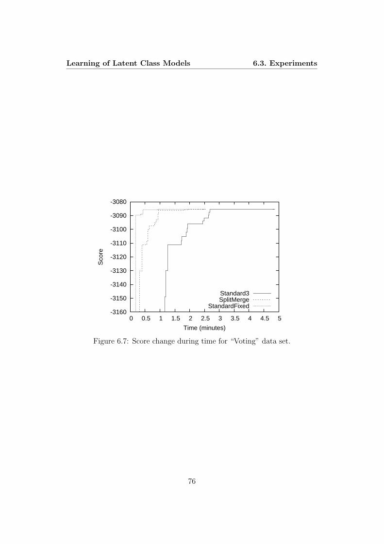
Learning of Latent Class Models 6.3. Experiments
-3160
-3150
-3140
-3130
-3120
-3110
-3100
-3090
-3080
0 0.5 1 1.5 2 2.5 3 3.5 4 4.5 5
Sco
re
Time (minutes)
Standard3SplitMerge
StandardFixed
Figure 6.7: Score change during time for “Voting” data set.
76

Learning of Latent Class Models 6.3. Experiments
6.3.4 Discussion
First, we look at the results for synthetic data. In the first series of tests (Ta-bles 6.1-6.7), SplitMerge was better than the standard algorithms for 3:3x3,10:7x2, and 10:10x2 models, that is when the number of possible configura-tions of the observed variables (i.e., of D1 × . . . × Dk) was around 1000 orsmaller. For small |D| the performance of different algorithms was similar,but for |D| around 105 and higher SplitMerge found higher scoring modelsthan the standard algorithms. Even though the running time of SplitMergewas higher than of Standard3, the comparison with StandardFixed shows thatSplitMerge was really better. For 10:15x2, 10:10x3, and 5:20x2 models (i.e.,when the number of possible configurations of the observed variables wasaround 30000 or larger) the performance of different algorithms was similar,but for large |D| Standard3 increased |H| a little faster than SplitMerge. Be-cause of this, for three data sets Standard3 found significantly better scoringmodels than SplitMerge.9 But as seen from Table 6.7, the performance ofthe algorithms was similar when they ran until they terminated themselves.One special case is |D| = 104 in Table 6.5, where the standard algorithmsfound better scoring models than SplitMerge and the algorithms terminatedthemselves. There, SplitMerge simply terminated in one of its five runs with a6–component model, because none of random splits led up to a better model.But as seen from Table 6.10, SplitMerge performed the same as the standardalgorithms for other random parameterisations of the 10:10x3 structure with|D| = 104.
In the second series of tests (Table 6.8) we see a similar pattern as in thefirst series: SplitMerge was better than the standard algorithms when thenumber of possible configurations of the observed variables was around 5000(model 10:2,3,4,5,6,7) or smaller, and the performance of the algorithms wassimilar otherwise (with Standard3 increasing |H| a little faster than Split-Merge for the 10:15x2 model).
In the third series of tests (Tables 6.9 and 6.10) we see that differentrandom parameterisations of the same generative structure generally did notmake a big difference in the performance of the algorithms.
In the fourth series of tests (Table 6.11), SplitMerge was better thanthe standard algorithms independently of the number of components in agenerative m:10x2 model (with the exception of the simplest case when m =2). Again the running time of SplitMerge was higher than of Standard3, butthe comparison with StandardFixed shows that SplitMerge was really better.
Now we discuss the results of the tests where m in StandardFixed was
9Even though for |D| = 105 in Table 6.4 |H| for SplitMerge is the same as |H| forStandard3, the final model contains only 6 components in most of the runs of SplitMerge.
77

Learning of Latent Class Models 6.3. Experiments
equal to the true |H|. We consider it normal that for those data sets where|H| given by SplitMerge was lower than the true |H|, setting m to the true|H| decreased the mean score for StandardFixed. This happened because|D| was probably not big enough to support models with more components.However, we were surprised that setting m to the true |H| decreased themean score for StandardFixed for two last data sets from Tables 6.1 and 6.2and the last data set from Table 6.3 as well. There, |H| given by SplitMergewas higher than the true |H|, that is SplitMerge overestimated the number ofcomponents. But it turns out that this overestimation was “reasonable” in asense that StandardFixed also prefers models with too many components.10
We think that such a behaviour was caused by the local maxima problemwhen estimating model parameters. It seems that increasing the number ofparameters by having too many components allows the EM algorithm to findbetter local maximum parameters.
As seen from Figures 6.1-6.3, Standard3 increases the model score a littlefaster than SplitMerge in the beginning, but in Figures 6.1 and 6.3 SplitMergefinds higher scoring models at the end. In Figure 6.2, Standard3 stops withhigher scoring models, but for |H| = 5 both Standard3 and SplitMerge foundthe same scoring models as StandardFixed.
We give a summary of our results for synthetic data in Table 6.16. Herewe show how did SplitMerge perform in comparison with Standard3 and Stan-dardFixed for given data set size (|D|) and number of possible configurationsof the observed variables (|D1 × . . .×Dk|).
|D| |D1 × . . .×Dk|Around 5000 or lower Around 30000 or higher
< 105 The algorithms performed similarly. The algorithms performed similarly.SplitMerge performed better The algorithms performed similarly,
≥ 105 than the standard algorithms. but Standard3 was a littlefaster than SplitMerge.
Table 6.16: A summary of the results for synthetic data.
Now we look at the results for real data. As seen from Table 6.13, theresults depend on the data set size. For all 9 data sets of size higher than4500, SplitMerge found better scoring models than Standard3. For all 11data sets of size lower than 4500, Standard3 found better scoring modelsthan SplitMerge (for 3 data sets) or the scores were similar (for 8 data sets).
10We made sure that the BIC score is not misleading by checking that for model M1
with true |H| and model M2 with too high |H| we have KL(PM2 , PG) < KL(PM1 , PG)when BIC (M2) > BIC (M1), where G is the generative model.
78

Learning of Latent Class Models 6.3. Experiments
When |D| > 4500, SplitMerge found significantly better scoring modelsthan Standard3 for 6 data sets. For most of these data sets, the algorithmsstopped because of the 5 hour time limit. But contrary to the results forsynthetic data, there is a big difference in |H| values of SplitMerge and ofStandard3 when the algorithms stop because of the time limit. So, SplitMergeincreased the cardinality faster then Standard3. We have also performed theexperiments where the number of starting points for EM in Standard3 wasset to 16 rather than 64. This way, Standard3 increased the cardinality fasterthan previously at a cost of worse parameters. In this setup, SplitMerge foundsignificantly better scoring models than Standard3 for 6 data sets again. Also,the results in Table 6.14 indicate that letting the algorithms run until theyterminate themselves does not cause SplitMerge to perform the same as thestandard algorithms. When |D| < 4500, Standard3 found significantly betterscoring models than SplitMerge for 1 data set.
As for StandardFixed, on average it performed a little better than Split-Merge.
For some data sets, the highest scoring models found by Standard3 andby SplitMerge have different |H|. For those 6 data sets where SplitMergefound significantly better scoring models than Standard3, |H| determinedby SplitMerge is much higher than |H| determined by Standard3. For“Pen” and “Shuttle”, Standard3 was simply unable to increase |H|. For“Adult”, “Mushroom”, “Satimage”, and “Spambase”, SplitMerge was fasterthan Standard, and both algorithms were stopped because of the time limit.For 4 more data sets (“Image”, “Letter”, “Credit”, and “Thyroid”), |H| de-termined by Standard3 and by SplitMerge differ by 1. In all of them, the bestmodel found by Standard has a higher score than the best model found bySplitMerge, even though for “Letter” and “Thyroid” SplitMerge performedbetter on average. This is related to the fact that generally the variance ofthe score is lower for SplitMerge than for Standard3.
The results in Table 6.15 show that the parameter adjustment operationis useful. For 7 data sets, it allowed to find better scoring models. For 4 outof those 7 data sets, it allowed to find significantly better scoring models. For3 data sets (“Page”, “Housing”, and “Vehicle”), it led to different |H|, whichquite interestingly was always lower by 1 than |H| determined by SplitMerge-NoAdjust. It was because after the parameter adjustment SplitMerge was ableto increase the score by performing the state merging operation. Only for 2data sets (“Audiology” and “Thyroid”), using the parameter adjustment didnot cause the score to improve while at the same time increasing “t” a little.
As for the component merging operation, it caused the score to improvefor 7 out of 16 data sets where it has been tried (for 4 out of 5, whenconsidering only the data sets of size higher than 4500). So, the component
79

Learning of Latent Class Models 6.3. Experiments
merging seems to be useful as well.As seen from Figures 6.4-6.7, models found by SplitMerge most of the time
have higher score than models found by Standard3. And usually, towards theend SplitMerge gets close to StandardFixed.
Similar results for real data have been obtained in the experiments fromSection 4.5. It may seem surprising that compared to the experiments fromthat section, where only the component splitting has been used, the param-eter reusing algorithm does not show more improvement over the standardalgorithms. However, the setup of the experiments from Section 4.5 and ofthe experiments here is quite different.
Summing up the results for both synthetic and real data, on average Split-Merge performed better than Standard3. It seems that SplitMerge becomesmore useful as |D| increases. Another advantage of SplitMerge is that thevariance of the score for it is lower than for Standard3. SplitMerge performeda little better than StandardFixed on synthetic data and a little worse onreal data. Since StandardFixed has the advantage of knowing the number ofcomponents, we consider this to be a good result.
Of course, very often SplitMerge still does not find the global maximumparameters. Indications of this are the situations where the variance of thescore for SplitMerge is not zero or models found by SplitMerge have lowerscore than models found by StandardFixed.
80

Chapter 7
Learning of Hierarchical LatentClass Models
In this chapter we extend our algorithm that learns LC models to hierarchicallatent class (HLC) models. Here we assume that the skeleton of an HLCmodel is fixed (that is, all the variables and edges between them are fixed)and the goal is to determine the cardinalities of hidden variables and modelparameters.
First, we extend the component splitting, component merging, and pa-rameter adjustment operations to HLC models. Then we describe the algo-rithms that learn the cardinalities and parameters in HLC models by eitherusing these extended operations or standard starting points for EM. Finally,we present experiments comparing the performance of these algorithms.
7.1 Parameter Reusing for HLC Models
In this section, we describe how parameters can be reused in HLC models.We reuse them by extending the component splitting, component merging,and parameter adjustment operations from Definitions 4.2 (page 22), 5.2(page 50), and 6.1 (page 57). The extensions are quite straightforward: eachoperation is performed on the root node in an HLC model. Below we giveformal definitions. For an HLC model M , LC (M) will denote the LC modelconsisting of the root node of M and all the child nodes of the root, with theprobability distributions for these nodes being the same as in M .
Definition 7.1 We say that HLC model M∗ is obtained from HLC modelM by splitting a component if LC (M∗) is obtained from LC (M) by splittinga component and the rest of M∗ and M are identical.
81

Learning of Hierarchical Latent Class Models 7.2. Algorithms
Definition 7.2 We say that HLC model M∗ is obtained from HLC model Mby merging two components if LC (M∗) is obtained from LC (M) by mergingtwo components and the rest of M∗ and M are identical.
Definition 7.3 We say that HLC model M ′ is obtained from HLC model Mby parameter adjustment if there exists HLC model M∗ such that:
• M∗ is obtained from M by splitting a component and then runningEM, and M ′ is obtained from M∗ by merging two components and thenrunning EM,or
• M∗ is obtained from M by merging two components and then runningEM, and M ′ is obtained from M∗ by splitting a component and thenrunning EM.
Here the EM algorithm updates all the parameters of an HLC model.1
All these three operations work with the root node of an HLC model.When performing parameter reusing for a non-root node, first we do rootwalking until the node of interest becomes the root and then we work withthis new root. So, by using the fact that root walking leads to an equivalentmodel, we restrict ourselves to working with the root node and this wayavoid the problem of considering the parents of a node when changing itscardinality.
We do not know about theoretical properties (like those from Sections 4.3and 5.3) of these operations for HLC models.
7.2 Algorithms
In this section, we discuss the algorithms that will be used in our experimentson learning the cardinalities and parameters in HLC models.
7.2.1 Algorithm Based on Splitting and Merging
In this section, we provide our algorithm that learns the cardinalities andparameters in HLC models by using the component splitting, component
1We do not define the parameter adjustment for HLC models by simply requiringLC (M ′) to be obtained from LC (M) by adjusting the parameters, because we allow theEM algorithm to update all the parameters of an HLC model, not only those attached tothe root and its child nodes.
82

Learning of Hierarchical Latent Class Models 7.2. Algorithms
merging, and parameter adjustment operations. Algorithm HLCSplitMergetakes training data D and model skeleton s as input and returns an HLCmodel. It tries to find an HLC model that is the best according to thefunction score, which can be any penalised likelihood scoring function. Thepseudocode of HLCSplitMerge is given in page 84. This algorithm is verysimilar to the SplitMerge algorithm (page 59). Only steps 1, 7, 20, and 31are changed. In step 1, the algorithm starts with the HLC model L wherethe cardinality of each hidden variable is one and the maximum likelihoodparameters are deterministically computed from D. In steps 7, 20, and 31,the procedures HLCSplit, HLCMerge, and HLCAdjust instead of the corre-sponding procedures for LC models are called. We will now describe thesethree procedures.
The procedure HLCSplit increments the cardinality of one hidden variablefrom an HLC model L. The pseudocode is given in page 85. The procedureincrements the cardinality of each hidden variable alone by making thatvariable the root, splitting a component as described in Definition 7.1, andrunning the EM algorithm. The model where incrementing the cardinalitygave the highest score is taken as the final one.
The procedure HLCMerge decrements the cardinality of one hidden vari-able from an HLC model L. The pseudocode is given in page 85. The proce-dure decrements the cardinality of each hidden variable alone by making thatvariable the root, merging two components as described in Definition 7.2, andrunning the EM algorithm. The model where decrementing the cardinalitygave the highest score is taken as the final one.
The procedure HLCAdjust tries to increase the score of an HLC model Lby performing the parameter adjustment operation. The pseudocode is givenin page 86. The procedure considers hidden variables one by one by making ahidden variable to be the root and then trying to improve model parameterssimilarly as in Adjust for LC models from page 62. The procedure terminateswithout considering other hidden variables as soon as a model giving anincrease in score higher than a positive parameter δ is found. Similarly as inAdjust, models L′ in step 3 and Ls in step 10 are not computed directly buttaken from the last run of HLCMerge and the last run of HLCSplit.
We can see that the algorithm HLCSplitMerge allows to have hidden vari-ables with cardinality 1. This is different from the approach of Zhang (2002);Zhang (2004), where the cardinality of a hidden variable can not be lowerthan 2. We allow the cardinality to be 1, because this provides a naturaloutset for the component splitting and because the algorithm can indicatethat a hidden node is not needed by making its cardinality 1 in the finalmodel. Strictly speaking, a model containing a hidden node with cardinality1 is no longer an HLC model, because it is equivalent to the model where this
83

Learning of Hierarchical Latent Class Models 7.2. Algorithms
Procedure 7.1 HLCSplitMerge(D, s)
1: Let L be the HLC model with skeleton s and the cardinality of eachhidden variable being one.
2: doPhase1 ← true, doPhase2 ← true.3: loop4: if doPhase1 then5: L0 ← L.6: repeat7: L′ ← HLCSplit(L,D).8: if score(L′) > score(L) then9: L ← L′.
10: end if11: until L 6= L′.12: if score(L) > score(L0) then13: doPhase2 ← true.14: end if15: doPhase1 ← false.16: end if17: if doPhase2 then18: L0 ← L.19: repeat20: L′ ← HLCMerge(L,D).21: if score(L′) > score(L) then22: L ← L′.23: end if24: until L 6= L′.25: if score(L) > score(L0) then26: doPhase1 ← true.27: end if28: doPhase2 ← false.29: end if30: if not doPhase1 and not doPhase2 then31: L′ ← HLCAdjust(L,D).32: if score(L′) > score(L) then33: L ← L′, doPhase1 ← true, doPhase2 ← true.34: else35: return L.36: end if37: end if38: end loop
84

Learning of Hierarchical Latent Class Models 7.2. Algorithms
Procedure 7.2 HLCSplit(L,D)
1: for each hidden variable Hi of L do2: Obtain from L the HLC model L∗ with Hi as the root by doing root
walking.3: Li ← Split(L∗,D), where the procedure Split is performed as in
page 60, but in each step (producing two-component models, data Ds,model Ls, running EM) working with HLC rather than LC models.
4: end for5: L′ ← arg maxLi
score(Li).6: return L′.
Procedure 7.3 HLCMerge(L,D)
1: for each hidden variable Hi of L do2: Obtain from L the HLC model L∗ with Hi as the root by doing root
walking.3: Li ← Merge(L∗,D), where the procedure Merge is performed as in
page 61, but in each step (producing model L∗, running EM) workingwith HLC rather than LC models.
4: end for5: L′ ← arg maxLi
score(Li).6: return L′.
85

Learning of Hierarchical Latent Class Models 7.2. Algorithms
Procedure 7.4 HLCAdjust(L,D)
1: for each hidden variable Hi of L do2: Obtain from L the HLC model L∗ with Hi as the root by doing root
walking.3: L′ ← Merge(L∗,D), with Merge performed as in step 3 of HLCMerge.4: L′′ ← Split(L′,D), with Split performed as in step 3 of HLCSplit.5: if score(L′′) > score(L) + δ then6: return L′′.7: else8: L ← ∅.9: for each component hs of L∗ do
10: Obtain an HLC model Ls as in the procedure Split from page 60,but in each step (producing two-component models, data Ds,model Ls, running EM) working with HLC rather than LC models.
11: for each pair of components {ha, hb} where ha is a new componentand hb is an old component of Ls do
12: Obtain model L′ by merging ha and hb in Ls.13: Add L′ to L.14: end for15: end for16: Obtain model L′′ by running the multiple restart EM with L as
starting points and data D.17: if score(L′′) > score(L) + δ then18: return L′′.19: end if20: end if21: end for22: return L.
86

Learning of Hierarchical Latent Class Models 7.2. Algorithms
hidden node and the adjacent edges are removed. Such a model partitionsthe observed variables into groups, where variables in different groups areassumed to be independent of each other.
Another difference from the approach of Zhang (2002); Zhang (2004) isthat we do not check whether the obtained models are regular. We allow thecardinality of a hidden variable to be higher than required in the definitionof a regular structure, because this may allow to perform the componentmerging later.
7.2.2 Algorithms Based on Standard Starting Points
Similarly as in the experiments with LC models, the algorithm HLCSplit-Merge will be compared with the algorithms that use standard startingpoints for EM. One of them, called HLCStandard3, has almost the samemain procedure as HLCSplitMerge (see page 84). HLCStandard3 also has3 phases: increasing cardinalities, decreasing cardinalities, and improvingparameters. The difference from HLCSplitMerge is that instead of callingHLCSplit, HLCMerge, and HLCAdjust it calls HLCIncrement, HLCDecre-ment, and HLCNewParams, the pseudocodes for which are given below.
HLCIncrement (page 87) increments the cardinality of each hidden vari-able alone and estimates model parameters by running EM from randomstarting points. The model where incrementing the cardinality gave thehighest score is taken as the final one. In the same pattern, HLCDecrement(page 88) decrements the cardinality of each hidden variable alone. HLC-NewParams (page 88) simply runs EM from random starting points. In allthese three procedures, |M| is specified in advance and random parametersare sampled from the uniform distribution.
Procedure 7.5 HLCIncrement(L,D)
1: for each hidden variable Hi of L do2: Let m be the structure of L, where the cardinality of Hi is increased
by 1.3: Produce a set M of HLC models having structure m and random
parameters.4: Obtain model Li by running the multiple restart EM with M as start-
ing points.5: end for6: L′ ← arg maxLi
score(Li).7: return L′.
87

Learning of Hierarchical Latent Class Models 7.2. Algorithms
Procedure 7.6 HLCDecrement(L,D)
1: for each hidden variable Hi of L where |Hi| > 1 do2: Let m be the structure of L, where the cardinality of Hi is decreased
by 1.3: Produce a set M of HLC models having structure m and random
parameters.4: Obtain model Li by running the multiple restart EM with M as start-
ing points.5: end for6: L′ ← arg maxLi
score(Li).7: return L′.
Procedure 7.7 HLCNewParams(L,D)
1: Let m be the structure of L.2: Produce a set M of HLC models having structure m and random pa-
rameters.3: Obtain model L′ by running the multiple restart EM with M as starting
points.4: if score(L′) > score(L) + δ then5: return L′.6: else7: return L.8: end if
88

Learning of Hierarchical Latent Class Models 7.3. Experiments
The algorithm HLCStandardFixed uses standard starting points for EMand estimates HLC model parameters when the model structure is fixed.Its pseudocode is given in page 89. In the same way as StandardFixed forLC models, it repeatedly tries to improve model parameters by running themultiple restart EM from random starting points. The algorithm is stoppedwhen it reaches a time limit, and then L contains the best model. Parametersof models from M are again sampled from the uniform distribution.
Procedure 7.8 HLCStandardFixed(D,m)
1: Let L be an HLC model having structure m and random parameters.2: N ← N0.3: loop4: Produce a set M of N models, where each model has structure m and
random parameters.5: Obtain model L′ by running the multiple restart EM with M as start-
ing points.6: if score(L′) > score(L) then7: L ← L′.8: end if9: N ← 2N .
10: end loop
7.3 Experiments
In this section, we describe the experiments where we compare the approachthat uses the component splitting and merging (algorithm HLCSplitMerge)with the approach that uses standard starting points (algorithms HLCStan-dard3 and HLCStandardFixed) for learning cardinalities and parameters inHLC models. First, we describe the setup of experiments. Then we give theresults for synthetic and for real data. Finally, we discuss the results.
7.3.1 Setup of Experiments
The setup of experiments is the same as for LC models, described in Sec-tion 6.3.1. In HLCIncrement, HLCDecrement, and HLCAdjust, |M| = 64.Contrary to the experiments with LC models, the algorithms are not stoppedbefore they terminate themselves. The model structure m in HLCStandard-Fixed is the structure of the best scoring model found by HLCSplitMerge for
89

Learning of Hierarchical Latent Class Models 7.3. Experiments
a given data set. The running time of HLCStandardFixed is equal to themean running time of HLCSplitMerge for a given data set.
The results are displayed in the same way as for LC models, except thatin the field “hidden” the cardinalities of all the hidden variables in the bestscoring model are shown (the cardinalities of the root, its children, and itsgrandchildren are separated by colons).
7.3.2 Results for Synthetic Data
In these experiments, training data D is always sampled from some HLCmodel. Forward sampling is used and D over observed variables is alwayscomplete. The generative HLC model is always parameterised randomly,with its parameters sampled from the uniform distribution. The skeleton ofthe generative HLC model is provided as a parameter to HLCSplitMerge andHLCStandard3.
In the first series of tests, we sampled D of size 104, 105, and 106 from thesame HLC model having the structure shown in Figure 7.1. The cardinality ofeach observed variable is 3. This structure is taken from Zhang (2004). Hereand in further figures, hidden variables are labelled with their cardinalities.
3
3
D1 D2 D3
D4 3
D5 D6 D7
Figure 7.1: Structure with 7 observed variables.
We performed the experiments with two different parameterisations of thestructure from Figure 7.1. The first model was parameterised as usually. Thesecond model was also parameterised as usually, but it was ensured that eachconditional probability distribution contains an element no smaller than 0.6.Also, it was ensured that in each conditional probability table, the largestelements for different states of the child variable do not all correspond to thesame state of the parent variable. The idea of such a setup is taken fromZhang (2004) and Zhang and Kocka (2004). The results of tests are shownin Tables 7.1 and 7.2.
In the second series of tests, we sampled D of size 104 from HLC mod-els having the structures shown in Figures 7.2 and 7.3. The cardinal-ity of each observed variable is again 3. These structures are taken from
90

Learning of Hierarchical Latent Class Models 7.3. Experiments
|D| HLCStandard3 HLCSplitMerge HLCStandardFixedscore t hidden score t hidden score
104 -71381.2 ± 2.6 58 2:3,2 -71380.3 ± 0.0 35 2:3,2 -71378.6 ± 1.1105 -712205.8 ± 5.8 71 2:3,2 -712200.7 ± 0.0 41 2:3,2 -712200.4 ± 1.3106 -7121968.5 ± 85.6 128 2:3,3 -7121953.3 ± 71.8 148 2:3,3 -7121863.8 ± 18.1
Table 7.1: Sampled from the first model with 7 observed variables.
|D| HLCStandard3 HLCSplitMerge HLCStandardFixedscore t hidden score t hidden score
104 -65824.5 ± 0.3 62 3:3,3 -65824.4 ± 0.0 43 3:3,3 -65824.1 ± 0.3105 -656733.5 ± 6.8 118 3:3,3 -656722.2 ± 0.7 158 3:3,3 -656721.4 ± 0.8106 -6557966.9 ± 47.8 186 3:3,3 -6557889.6 ± 0.0 413 3:3,3 -6557887.5 ± 0.9
Table 7.2: Sampled from the second model with 7 observed variables.
Zhang and Kocka (2004). Models were parameterised in the same way asthe second model from the first series of tests. The results of tests are
2
2
3
D1 D2 D3
3
D4 D5 D6
2
3
D7 D8 D9
3
D10 D11 D12
Figure 7.2: Structure with 12 observed variables.
shown in Table 7.3. The field “t” indicates the rounded mean running timein hours. For the 18-variable model, each algorithm was run only 2 timesbecause of long running time.
Similarly as in the experiments with LC models, we display how the meanscore changes during time for several data sets. It is shown in Figures 7.4-7.8(bars at the end indicate 95% confidence intervals for the mean).
91

Learning of Hierarchical Latent Class Models 7.3. Experiments
3
2
3
D1 D2 D3
3
D4 D5 D6
2
3
D7 D8 D9
3
D10 D11 D12
2
3
D13 D14 D15
3
D16 D17 D18
Figure 7.3: Structure with 18 observed variables.
k HLCStandard3 HLCSplitMerge HLCStandardFixedscore t hidden score t hidden score
12 -108271.5 ± 52.8 77 1:2,2: -108302.8 ± 0.0 29 1:1,2: -108301.8 ± 0.13,3,3,3 2,2,3,3
18 -166025.7 ± 0.3 414 2:2,2,2: -166031.2 ± 0.0 289 2:2,2,2: -166030.1 ± 0.13,3,3,3,3,3 2,3,3,3,3,3
Table 7.3: Sampled from models with 12 and with 18 observed variables.
-7122500
-7122400
-7122300
-7122200
-7122100
-7122000
-7121900
-7121800
0 20 40 60 80 100 120 140 160 180
Sco
re
Time (minutes)
HLCStandard3HLCSplitMerge
HLCStandardFixed
Figure 7.4: Score change during time for data sampled from the first modelwith 7 observed variables, |D| = 106.
92

Learning of Hierarchical Latent Class Models 7.3. Experiments
-66500
-66400
-66300
-66200
-66100
-66000
-65900
-65800
0 10 20 30 40 50 60 70
Sco
re
Time (minutes)
HLCStandard3HLCSplitMerge
HLCStandardFixed
Figure 7.5: Score change during time for data sampled from the second modelwith 7 observed variables, |D| = 104.
-6558500
-6558400
-6558300
-6558200
-6558100
-6558000
-6557900
-6557800
0 50 100 150 200 250 300 350 400 450
Sco
re
Time (minutes)
HLCStandard3HLCSplitMerge
HLCStandardFixed
Figure 7.6: Score change during time for data sampled from the second modelwith 7 observed variables, |D| = 106.
93

Learning of Hierarchical Latent Class Models 7.3. Experiments
-109000
-108900
-108800
-108700
-108600
-108500
-108400
-108300
-108200
0 10 20 30 40 50 60 70 80
Sco
re
Time (hours)
HLCStandard3HLCSplitMerge
HLCStandardFixed
Figure 7.7: Score change during time for data sampled from the model with12 observed variables.
-167000
-166800
-166600
-166400
-166200
-166000
0 50 100 150 200 250 300 350 400 450
Sco
re
Time (hours)
HLCStandard3HLCSplitMerge
HLCStandardFixed
Figure 7.8: Score change during time for data sampled from the model with18 observed variables.
94

Learning of Hierarchical Latent Class Models 7.3. Experiments
7.3.3 Results for Real Data
For training data, we used the CoIL Challenge 2000 (van der Put-ten and van Someren (eds), 2000) data, preprocessed as described inZhang and Kocka (2004). The preprocessed data set contains 42 vari-ables and has size 5822. Most of the variables are binary. The struc-ture of the best HLC model for this data set found by the algorithm ofZhang and Kocka (2004) is shown in Figure 7.9. For hidden variables, thename of a variable and its cardinality are shown. For observed variables, thename of a variable is shown.
The skeleton from Figure 7.9 was provided as an input to HLCSplitMergeand HLCStandard3. The results of tests are shown in Table 7.4. The field“t” indicates the rounded mean running time in hours. Each algorithm wasrun only 2 times because of long running time. The cardinalities of hidden
HLCStandard3 HLCSplitMerge HLCStandardFixedscore t score t score
-51626.1 ± 7.4 971 -51516.5 ± 19.4 467 -51515.1 ± 30.1
Table 7.4: Results for CoIL data set.
variables in the final models found by HLCSplitMerge and HLCStandard3were the same as the cardinalities in Figure 7.9 except for the followingdifferences. For HLCStandard3, the cardinalities of h8, h20, and h21 werelower by 1 in the first run (model score -51621.8), and the cardinalities of h0,h20, and h21 were lower by 1 in the second run (model score -51630.3). ForHLCSplitMerge, the cardinality of h21 was higher by 1 in the first run (modelscore -51527.5), and all the cardinalities were the same as in Figure 7.9 inthe second run (model score -51505.5). The scores of the final models foundby HLCStandardFixed were -51497.9 and -51532.2.
In Figure 7.10, we display how the mean score changes during time (barsat the end indicate 95% confidence intervals for the mean).
95

h0(5
)
v59
v80
h3(2
)
v55
v76
h4(2
)
v57
v78
h5(2
)
v56
v77
h6(2
)
v44
v65
h7(2
)
v63
v84
h8(4
)
h9(2
)
v54
v75
h10(2
)
v70
v49
h11(2
)
v83
v62
h12(3
)
v47
v68
v86
h13(2
)
v64
v85
h14(2
)
v61
v82
h1(2
)
v45
v66
h2(2
)
v48
v69
h15(2
)
h16(2
)
v46
v67
h17(2
)
v58
v79
h18(2
)
v72
v51
h19(2
)
v53
v74
h20(3
)
v73
v52
h21(9
)
v05
v43
v04
Fig
ure
7.9:
HLC
model
stru
cture
for
CoI
Ldat
ase
t.
96

Learning of Hierarchical Latent Class Models 7.3. Experiments
-54500
-54000
-53500
-53000
-52500
-52000
-51500
0 100 200 300 400 500 600 700 800 900 1000
Sco
re
Time (hours)
HLCStandard3HLCSplitMerge
HLCStandardFixed
Figure 7.10: Score change during time for CoIL data set.
97

Learning of Hierarchical Latent Class Models 7.3. Experiments
7.3.4 Discussion
First, we look at the results for synthetic data. For data with 7 observedvariables (Tables 7.1 and 7.2), the final models found HLCSplitMerge havehigher score than the final models found by HLCStandard3, especially for|D| higher than 104. The structures of the best final models found by bothalgorithms are the same. For data with 12 and with 18 observed variables(Table 7.3), the results are the opposite: the final models found by HLC-SplitMerge have lower score than the final models found by HLCStandard3.This is because HLCStandard3 was able to increase the cardinalities moreand this way the structure of its final best model is closer to the structure ofthe generative model (as seen from the fields “hidden” in Table 7.3).
When comparing HLCSplitMerge with HLCStandardFixed, we see thatthe average final score was always higher for HLCStandardFixed (and some-times it was even significantly better), but the difference in the average finalscores was really big for one data set only (namely, the last one from Ta-ble 7.1). So, usually the parameters found by HLCSplitMerge were onlya little worse than those find by HLCStandardFixed for given HLC modelstructures.
Figures 7.7 and 7.8 show that for the two data sets where HLCSplit-Merge found worse models than HLCStandard3, HLCSplitMerge was abouttwo times faster, and only because of longer running time HLCStandard3found better models.
Now we look at the results for real data. As seen from Table 7.4 andFigure 7.10, HLCSplitMerge performed much better than HLCStandard3.And as described at the end of Section 7.3.3, the structures found by HLC-SplitMerge are closer to the structure from Figure 7.9. Having in mind theresults for synthetic data, it is interesting that this time HLCSplitMergeended up with higher cardinalities for some variables than HLCStandard3.As for the HLCStandardFixed algorithm, we see that it finds similarly scor-ing models as HLCSplitMerge: for the structure where the model score was-51505.5 for HLCSplitMerge, it was -51497.9 and -51532.2 in the two runsof HLCStandardFixed. It is interesting to compare that the BIC score ofthe best model found by the HSHC algorithm (described in Section 3.4.2) ofZhang and Kocka (2004) was -51465.2 It took 121 hours to learn this modelusing a processor that has a similar rate as in our experiments. So, theHSHC algorithm, which learns the model skeleton as well, learned better pa-rameters than HLCStandardFixed and HLCSplitMerge. The reason for thismay be that in HSHC running local EM rather than EM that updates all the
2We remind that this model has the same structure as the one discovered by HLCSplit-Merge and used by HLCStandardFixed.
98
Learning of Hierarchical Latent Class Models 7.3. Experiments
parameters of a model causes not only to save time but also to find better pa-rameters. We believe that HLCSplitMerge can be improved by running localEM after splitting or merging components, and only after that running EMthat updates all the parameters of a model. In local EM, only the probabilitydistributions for the root node and its children would be optimised.
Both in the experiments with synthetic and with real data, the parame-ter adjustment operation (procedure HLCAdjust) often increased the modelscore. But the component merging operation (procedure HLCMerge) in-creased the model score only once (in one of the runs for real data). Thereason for this may be that in our experiments the cardinalities of hiddenvariables in the optimal HLC models are not high, and in this case the com-ponent splitting usually does not overestimate the cardinality.
So, on average HLCSplitMerge performed a little better than HLCStan-dard3 on synthetic data, and it performed much better than HLCStandard3on real data. For synthetic data, the variance of the score for HLCSplit-Merge was lower than for HLCStandard3. For both synthetic and real data,the score of models found by HLCSplitMerge was close to the score of modelsfound by HLCStandardFixed. As mentioned above, a promising future workwould be the introduction of local EM in HLCSplitMerge.
99
Chapter 8
Conclusions and ResearchDirections
In this thesis, we have addressed the problem of learning Bayesian networkswith hidden variables. We have concentrated on a sub-problem of learn-ing the cardinalities of hidden variables and the parameters in latent class(LC) and hierarchical latent class (HLC) models. These models are tree-structured Bayesian networks with categorical variables and are among thesimplest types of Bayesian networks with hidden variables. The standardmethod for learning cardinalities and parameters is to run the EM algorithmfrom random starting points. We have proposed a method where startingpoints for EM are obtained by reusing the parameters of the already learnedmodels. When we reuse the parameters by performing the so-called com-ponent splitting operation, we increase the cardinality of a hidden variable.When we reuse the parameters by performing the so-called component merg-ing operation, we decrease the cardinality of a hidden variable. By repeatedlyperforming these operations, we learn both the cardinalities of hidden vari-ables and the parameters at the same time. We have proved that if some datais not described perfectly by some LC model, then with probability 1 it ispossible to increase the log-likelihood of that data by splitting a componentin that LC model (Theorem 4.2 on page 28). Based on experimental resultswe have conjectured that if some data over binary variables is describedperfectly by an LC model having one component more than the generativemodel for that data, then the generative model can be obtained by mergingtwo components of that model, provided that the dimension of that modelis not higher than the complete dimension of that data (Conjecture 5.2 onpage 53).
In the experiments with LC and HLC models, our algorithms based oncomponent splitting and merging in a majority of cases performed better than
100

Conclusions and Research Directions
the algorithms that use standard starting configurations for EM. In particu-lar, the parameter reusing approach was better for bigger-sized training data.However, we think that our algorithms can still be improved.
One possible improvement could be to introduce criteria for selectingthe most promising components for splitting and merging as it has beendone by Ueda et al. (2000) for continuous data (Section 3.3). For exam-ple, component hs from model L could be considered for splitting when thedistance between the distribution specified by the parameters of the com-ponent and the empirical distribution given by Ds is large. That is, whenKL
(PL(D1|hs) · . . . · PL(Dk|hs), PDs(D1, . . . , Dk)
)is large. Components hs
and ht could be considered for merging when the distance between the em-pirical distributions given by Ds and Dt is small.1
Another possible improvement would deal with the implementation ofcomponent splitting. Currently, we split a component randomly. It may beworth trying to compute from data a good direction for splitting. One maytry to improve the deterministic approaches suggested in Section 4.4.2.
For HLC models only, the main improvement should be introduction oflocal EM, as discussed in Section 7.3.4.
As discussed in Section 3.1.3, the scoring functions we use are not com-pletely suited for networks with hidden variables. It would be interestingto see if using better suited scoring functions would change the performanceof the algorithms. The first step here could be using a modified BIC scorewhere effective dimension of a Bayesian network and relabeling of states ofhidden variables (see Section 3.1.3) are taken into account.
In this thesis, we first proposed a parameter reusing approach for LCmodels and after that extended it to HLC models. A natural next step wouldbe to move from tree-structured models to unrestricted Bayesian networkswith hidden variables. The main issue here is how to define component (i.e.,state) splitting and merging for hidden variables that have parents. The mostobvious extension of Definitions 4.2 (page 22) and 5.2 (page 50) would bethe following. For a hidden variable H with parents A1, . . . , Aj and childrenB1, . . . , Bk in model M , producing of model M∗ by splitting of state hs intoh1
s and h2s would mean setting PM∗(h1
s|a) = PM∗(h2s|a) = 1
2PM(hs|a) for
every configuration a of A1, . . . , Aj, and setting PM∗(Bi|h1s) and PM∗(Bi|h2
s)to be close to PM(Bi|hs), ∀i = 1, . . . , k. Producing of model M∗ by mergingof states h1
s and h2s into hs would mean setting PM∗(hs|a) = PM(h1
s|a) +PM(h2
s|a) for every configuration a of A1, . . . , Aj, and setting PM∗(Bi|hs) =
1Measuring the distance between the distributions specified by the parameters of com-ponents hs and ht could be computationally too expensive because each of these distribu-tions may contain
∏ki=1 |Di| non-zero probabilities.
101

Conclusions and Research Directions
PM (h1s)
PM∗ (hs)PM(Bi|h1
s) + PM (h2s)
PM∗ (hs)PM(Bi|h2
s), ∀i = 1, . . . , k, where PM(h1s), PM(h2
s),
and PM∗(hs) are marginal probabilities of states of H according to modelsM and M∗. However, state splitting defined in this way has an undesirableproperty of working differently for equivalent models. For example, considerthe Bayesian networks A → H → B and A ← H → B, where H is hiddenand A,B are observed variables. These two models are equivalent. Forthe first model, the probability distributions P (A, h1
s) and P (A, h2s) after
splitting would be identical, while for the second model not. This could berepaired (i.e., the distributions forced to be different for the first model aswell) by setting during splitting PM∗(h1
s|a) = 12PM(hs|a)+εa and PM∗(h2
s|a) =12PM(hs|a)−εa for every configuration a of A1, . . . , Aj, where each εa is a real
number close to zero. For models containing more than one hidden variable,the easiest way of optimising the cardinalities seems to be the one used inHLC models: increasing or decreasing the cardinality of one variable at a timewhile keeping the cardinalities of other hidden variables fixed. When testingthis parameter reusing approach, the first step could be to perform tests withhierarchical naive Bayes (HNB) models (Zhang et al., 2004), which are likeHLC models except that the root variable (i.e., class variable) is observed.HNB models are not as complex a unrestricted Bayesian networks, but atthe same time contain hidden variables that have an observed parent.
We reuse the parameters by performing component splitting and merging.As discussed in the beginning of Chapters 4 and 5, the parameters could alsobe reused by performing component introduction and removal. Working onalgorithms that would use these two operations instead of (or in addition to)splitting and merging could be yet another research direction.
A more theoretical research would be further investigation of propertiesof component merging in LC models.
Concerning practical usage, one could consider another application of theparameter reusing technique. In this thesis, we have assumed a completelyautomatic learning where the algorithm learns the cardinalities and parame-ters by using training data alone as input. However, there may be situationswhere a model for given training data is already available and the goal isto improve the available model rather than to find the model that describestraining data the best. In such a case, the parameter reusing approach thatwould use the available model as the initial one would be very convenient be-cause it would not forget the parameters of the available model while tryingto find better models.
102

Appendix A
Preprocessing of Text Data
In this appendix, we describe how we preprocessed text data, which was usedthen in the experiments from Section 4.5. The description here is based onpages 29-30 of Karciauskas (2002).
The Reuters-21578 text categorisation test collection (Distribution 1.0)(Lewis, 1997) is a widely used test collection for text categorisation research.It contains about 20000 documents (Reuters news stories), each of themassigned to zero or more topics. We used the most popular “ModApte” splitof this collection into training and test sets. Following the test setup ofYang and Liu (1999), we selected the topics that have at least one documentboth in the training set and the test set. It resulted in selecting 90 topics.After eliminating documents that do not belong to any of these 90 topics,we got a training set of 7769 documents and a test set of 3018 documents.
When preprocessing documents, for simplicity we did not distinguish be-tween text that appears in the title and text that appears in the body of adocument. First, for the extraction of features from a document, we con-verted text to lowercase and selected from it words (i.e., sequences of alphasymbols delimited by any other symbols). Then we removed function words(i.e. topic-neutral words such as articles, prepositions). After this prepro-cessing, each document had a number of features – the non-function wordsappearing in the document. A feature set was then built by taking from thedocuments in the training set all the features except those that appear onlyin one document. The feature set consists of 15715 words. As in many otherworks on text categorisation, we used binary features.
Since for many machine learning algorithms it is computationally impos-sible to use 15715 features, we performed feature selection. For this, we usedthe information gain criteria, because it has been reported as one of the mosteffective by Yang and Pedersen (1997). For each topic, a separate set of themost relevant features was selected.
103

Preprocessing of Text Data
For the experiments from Section 4.5, we produced 9 different data sets:for topics Earn, Crude, and Corn, with 10, 20, and 30 features for eachtopic. For these experiments, we merged the training and test sets into oneset, giving the data of size 10787.
104

Bibliography
G. Ball and D. Hall. 1967. A clustering technique for summarizing multi-variate data. Behavioral Science, 12:153–155.
Y. Barash and N. Friedman. 2001. Context-specific Bayesian clusteringfor gene expression data. In RECOMB ’01: Proceedings of the fifth annualinternational conference on Computational biology, pages 12–21.
E. Bauer, D. Koller, and Y. Singer. 1997. Update rules for parameterestimation in Bayesian networks. In Uncertainty in Artificial Intelligence:Proceedings of the Thirteenth Conference, pages 3–13.
M. J. Beal and Z. Ghahramani. 2003. The variational Bayesian EM al-gorithm for incomplete data: with application to scoring graphical modelstructures. Bayesian Statistics, 7:453–464.
J. Binder, D. Koller, S. J. Russell, and K. Kanazawa. 1997. Adaptiveprobabilistic networks with hidden variables. Machine Learning, 29(2-3):213–244.
C. L. Blake and C. J. Merz. 1998. UCI repository of machine learningdatabases. http://www.ics.uci.edu/∼mlearn/MLRepository.html.
K. Blekas and A. Likas. 2004. Incremental mixture learning for clusteringdiscrete data. In Methods and Applications of Artificial Intelligence, ThirdHelenic Conference on AI, SETN 2004, pages 210–219.
X. Boyen, N. Friedman, and D. Koller. 1999. Discovering the hidden struc-ture of complex dynamic systems. In Uncertainty in Artificial Intelligence:Proceedings of the Fifteenth Conference, pages 91–100.
P. S. Bradley, U. M. Fayyad, and C. A. Reina. 1998. Scaling EM(Expectation-Maximization) clustering to large databases. Technical Re-port MSR-TR-98-35, Microsoft Research.
105

BIBLIOGRAPHY
M. Brand. 1999. Structure learning in conditional probability modelsvia an entropic prior and parameter extinction. Neural Computation,11(5):1155–1182.
G. Celeux, S. Chretien, F. Forbes, and A. Mkhadri. 2001. A component-wise EM algorithm for mixtures. Journal of Computational and GraphicalStatistics, 10(4):699–712.
P. Cheeseman and J. Stutz. 1995. Bayesian classification (AutoClass):Theory and results. In Advances in Knowledge Discovery and Data Mining,pages 153–180. AAAI Press.
D. M. Chickering and D. Heckerman. 1997. Efficient approximations for themarginal likelihood of Bayesian networks with hidden variables. MachineLearning, 29(2-3):181–212.
D. M. Chickering. 2002. Optimal structure identification with greedysearch. The Journal of Machine Learning Research, 3:507–554.
C. Chow and C. Liu. 1968. Approximating discrete probability distribu-tions with dependence trees. IEEE Transactions on Information Theory,14(3):462–467.
D. Connolly. 1993. Constructing hidden variables in Bayesian networksvia conceptual clustering. In Machine Learning, Proceedings of the TenthInternational Conference, pages 65–72.
G. F. Cooper and E. Herskovits. 1992. A Bayesian method for the induc-tion of probabilistic networks from data. Machine Learning, 9(4):309–347.
G. F. Cooper. 1995. A Bayesian method for learning belief networksthat contain hidden variables. Journal of Intelligent Information Systems,4(1):71–88.
A. Dempster, N. Laird, and D. Rubin. 1977. Maximum likelihood fromincomplete data via the EM algorithm. Journal of the Royal StatisticalSociety, 39(B):1–38.
G. Elidan and N. Friedman. 2001. Learning the dimensionality of hid-den variables. In Uncertainty in Artificial Intelligence: Proceedings of theSeventeenth Conference, pages 144–151.
G. Elidan and N. Friedman. 2003. The Information Bottleneck EM algo-rithm. In Uncertainty in Artificial Intelligence: Proceedings of the Nine-teenth Conference, pages 200–208.
106

BIBLIOGRAPHY
G. Elidan, N. Lotner, N. Friedman, and D. Koller. 2000. Discoveringhidden variables: A structure-based approach. In Proceedings of the 13thAnnual Conference on Neural Information Processing Systems, pages 479–485.
G. Elidan, M. Ninio, N. Friedman, and D. Schuurmans. 2002. Data pertur-bation for escaping local maxima in learning. In Proceedings of the Eigh-teenth National Conference on Artificial Intelligence and Fourteenth Con-ference on Innovative Applications of Artificial Intelligence (AAAI/IAAI),pages 132–139.
U. M. Fayyad, C. A. Reina, and P. S. Bradley. 1998. Initialization ofiterative refinement clustering algorithms. In Proceedings of the 4th In-ternational Conference on Knowledge Discovery and Data Mining, pages194–198.
M. A. T. Figueiredo and A. K. Jain. 2002. Unsupervised learning of finitemixture models. IEEE Transactions on Pattern Analysis and MachineIntelligence, 24(3):381–396.
J. Fischer and K. Kersting. 2003. Scaled CGEM: A fast accelerated EM.In Machine Learning: ECML 2003, 14th European Conference on MachineLearning, pages 133–144.
D. H. Fisher. 1987. Knowledge acquisition via incremental conceptualclustering. Machine Learning, 2(2):139–172.
N. Friedman. 1997. Learning belief networks in the presence of miss-ing values and hidden variables. In Proceedings of the 14th InternationalConference on Machine Learning, pages 125–133.
N. Friedman. 1998. The Bayesian structural EM algorithm. In Uncertaintyin Artificial Intelligence: Proceedings of the Fourteenth Conference, pages129–138.
D. Geiger, D. Heckerman, and C. Meek. 1996. Asymptotic model selectionfor directed networks with hidden variables. In Uncertainty in ArtificialIntelligence: Proceedings of the Twelfth Conference, pages 283–290.
D. Geiger, D. Heckerman, H. King, and C. Meek. 2001. Stratified exponen-tial families: Graphical models and model selection. Annals of Statistics,29(2):505–529.
107

BIBLIOGRAPHY
S. Geman and D. Geman. 1984. Stochastic relaxation, Gibbs distributions,and the Bayesian restoration of images. IEEE Transactions on PatternAnalysis and Machine Intelligence, 6(6):721–741.
F. Glover and M. Laguna. 1993. Tabu search. In Modern HeuristicTechniques for Combinatorial Problems.
L. A. Goodman. 1974. Exploratory latent structure analysis using bothidentifiable and unidentifiable models. Biometrika, 61:215–231.
D. Haughton. 1988. On the choice of a model to fit data from an expo-nential family. Annals of Statistics, 16:342–355.
D. Heckerman. 1995. A tutorial on learning with Bayesian networks.Technical Report MSR-TR-95-06, Microsoft Research.
M. Jamshidian and R. I. Jennrich. 1997. Acceleration of the EM algorithmby using Quasi-Newton methods. Journal of the Royal Statistical Society:Series B (Statistical Methodology), 59(3):569–587.
F. V. Jensen, S. L. Lauritzen, and K. G. Olesen. 1990. Bayesian updatingin causal probabilistic networks by local computations. ComputationalStatistics Quaterly, 4:269–282.
G. Karciauskas, F. V. Jensen, and T. Kocka. 2004a. Parameter reusingin learning latent class models. In Eighth International Symposium onArtificial Intelligence and Mathematics.
G. Karciauskas, T. Kocka, F. V. Jensen, P. Larranaga, and J. A. Lozano.2004b. Learning of latent class models by splitting and merging compo-nents. In Second Workshop on Probabilistic Graphical Models.
G. Karciauskas. 2002. Text categorization using hierarchical Bayesiannetwork classifiers. MSc Thesis. Aalborg University.
S. Kirkpatrick, C. D. Gelatt, and M. P. Vecchi. 1983. Optimization bysimulated annealing. Science, 220:671–680.
T. Kocka and N. Zhang. 2002. Dimension correction for hierarchical latentclass models. In Uncertainty in Artificial Intelligence: Proceedings of theEighteenth Conference, pages 267–274.
C.-K. Kwoh and D. F. Gillies. 1996. Using hidden nodes in Bayesiannetworks. Artificial Intelligence, 88(1-2):1–38.
108

BIBLIOGRAPHY
S. L. Lauritzen. 1995. The EM algorithm for graphical association modelswith missing data. Computational Statistics and Data Analysis, 19:191–201.
P. F. Lazarsfeld and N. W. Henry. 1968. Latent Structure Analysis. Boston:Houghton Mifflin.
D. D. Lewis. 1997. Reuters-21578 text categorization test collection.http://www.daviddlewis.com/resources/testcollections/reuters21578.
L. Liu, D. C. Wilkins, X. Ying, and Z. Bain. 1990. Minimum error treedecomposition. In Uncertainty in Artificial Intelligence: Proceedings of theSixth Conference, pages 180–185.
D. Madigan and J. York. 1995. Bayesian graphical models for discretedata. International Statistical Review, 63:215–232.
J. Martin and K. VanLehn. 1995. Discrete factor analysis: Learninghidden variables in Bayesian networks. Technical report, Department ofComputer Science, University of Pittsburgh.
Geoffrey J. McLachlan and Thriyambakam Krishnan. 1997. The EMAlgorithm and Extensions. John Wiley and Sons.
C. Meek, B. Thiesson, and D. Heckerman. 2002. Staged mixture modellingand boosting. In Uncertainty in Artificial Intelligence: Proceedings of theEighteenth Conference, pages 335–343.
C. Meek. 1997. Graphical models: selecting causal and statistical models.Ph.D. thesis, Carnegie Mellon University.
M. Meila and D. Heckerman. 1998. An experimental comparison of severalclustering and initialization methods. In Uncertainty in Artificial Intelli-gence: Proceedings of the Fourteenth Conference, pages 386–395.
X.-L. Meng and D. van Dyk. 1997. The EM algorithm – an old folk-songsung to a fast new tune. Journal of the Royal Statistical Society: Series B(Statistical Methodology), 59(3):511–567.
C. Montacie, M.-J. Caraty, and C. Barras. 1996. Mixture splitting technicand temporal control in a HMM-based recognition system. In Proceedingsof the International Conference on Spoken Language Processing, volume 2,pages 977–980.
109

BIBLIOGRAPHY
A. Moore. 1999. Very fast EM-based mixture model clustering usingmultiresolution kd-trees. In Advances in Neural Information ProcessingSystems 11, pages 543–549.
R. Neal and G. Hinton. 1998. A view of the EM algorithm that justifiesincremental, sparse, and other variants. In M. I. Jordan, editor, Learningin Graphical Models, pages 355–368.
R. E. Neapolitan. 2003. Learning Bayesian Networks. Prentice Hall.
NorsysSoftwareCorp. 2005. Tutorial on Bayesian Networks with Netica.http://www.norsys.com/tutorials/netica/secD/tut D1.htm.
L. Ortiz and L. Kaelbling. 1999. Accelerating EM: An empirical study. InUncertainty in Artificial Intelligence: Proceedings of the Fifteenth Confer-ence, pages 512–521.
M. Ostendorf and H. Singer. 1997. HMM topology design using maxi-mum likelihood successive state splitting. Computer Speech and Language,11(1):17–41.
J. Pearl. 1986. Fusion, propagation, and structuring in belief networks.Artificial Intelligence, 29(3):241–288.
J. Pearl. 1988. Probabilistic Reasoning in Intelligent Systems: Networksof Plausible Inference. Morgan Kaufmann Publishers Inc.
S. Ramachandran and R. J. Mooney. 1998. Theory refinement for Bayesiannetworks with hidden variables. In Proceedings of the 15th InternationalConference on Machine Learning, pages 454–462.
S. Richardson and P. J. Green. 1997. On Bayesian analysis of mixtureswith an unknown number of components. Journal of the Royal StatisticalSociety: Series B, 59(4):731–758.
D. Rusakov and D. Geiger. 2003. Automated analytic asymptotic eval-uation of the marginal likelihood for latent models. In Uncertainty inArtificial Intelligence: Proceedings of the Nineteenth Conference, pages501–508.
R. Salakhutdinov and S. T. Roweis. 2003. Adaptive overrelaxed boundoptimization methods. In Machine Learning, Proceedings of the TwentiethInternational Conference (ICML 2003), pages 664–671.
110

BIBLIOGRAPHY
G. Schwarz. 1978. Estimating the dimension of a model. Annals of Statis-tics, 6(2):461–464.
P. Spirtes, C. Glymour, and R. Scheines. 1993. Causation, Prediction, andSearch. Springer-Verlag.
P. Spirtes, C. Glymour, and R. Scheines. 2000. Causation, Prediction, andSearch. The MIT Press, 2 edition.
B. Stenger, V. Ramesh, N. Paragios, F. Coetzee, and J. M. Buhmann.2001. Topology free hidden Markov models: Application to backgroundmodeling. In Proceedings of the Eighth International Conference On Com-puter Vision, pages 294–301.
A. Stolcke and S. M. Omohundro. 1994. Inducing probabilistic grammarsby bayesian model merging. In Grammatical Inference and Applications,Second International Colloquium, pages 106–118.
J. Takami and S. Sagayama. 1992. A successive state splitting algo-rithm for efficient allophone modeling. In Proceedings of the InternationalConference on Acoustics, Speech, and Signal Processing, volume 1, pages573–576.
B. Thiesson, C. Meek, and D. Heckerman. 1999. Accelerating EM for largedatabases. Technical Report MSR-TR-99-31, Microsoft Research.
B. Thiesson. 1995. Accelerated quantification of Bayesian networks withincomplete data. In Proceedings of the First International Conference onKnowledge Discovery and Data Mining, pages 306–311.
J. Tian and J. Pearl. 2002. On the testable implications of causal modelswith hidden variables. In Uncertainty in Artificial Intelligence: Proceedingsof the Eighteenth Conference, pages 519–527.
J. Uebersax. 2000. A brief study of lo-cal maxima solutions in latent class analysis.http://ourworld.compuserve.com/homepages/jsuebersax/local.htm.
J. Uebersax. 2001. LCA frequently asked questions.http://ourworld.compuserve.com/homepages/jsuebersax/faq.htm.
N. Ueda and Z. Ghahramani. 2002. Bayesian model search for mix-ture models based on optimizing variational bounds. Neural Networks,15(10):1223–1241.
111

BIBLIOGRAPHY
N. Ueda, R. Nakano, Z. Ghahramani, and G. E. Hinton. 2000. SMEMalgorithm for mixture models. Neural Computation, 12(9):2109–2128.
P. van der Putten and M. van Someren (eds). 2000. CoIL Challenge 2000:The Insurance Company Case. Published by Sentient Machine Research,Amsterdam. Also a Leiden Institute of Advanced Computer Science Tech-nical Report 2000-09.
J. J. Verbeek, N. Vlassis, and B. Krose. 2003. Efficient greedy learning ofGaussian mixture models. Neural Computation, 15(2):469–485.
N. Vlassis and A. Likas. 2002. A greedy EM algorithm for Gaussianmixture learning. Neural Processing Letters, 15(1):77–87.
Y. Yang and X. Liu. 1999. A re-examination of text categorization meth-ods. In Proceedings of the 22nd Annual International ACM SIGIR Confer-ence on Research and Development in Information Retrieval, pages 42–49.
Y. Yang and J. O. Pedersen. 1997. A comparative study on feature selec-tion in text categorization. In Proceedings of the Fourteenth InternationalConference on Machine Learning, pages 412–420.
N. L. Zhang and T. Kocka. 2004. Efficient learning of hierarchical la-tent class models. In 16th IEEE International Conference on Tools withArtificial Intelligence (ICTAI 2004), pages 585–593.
N. L. Zhang, T. D. Nielsen, and F. V. Jensen. 2004. Latent variable discov-ery in classification models. Artificial Intelligence in Medicine, 30(3):283–299.
N. L. Zhang. 1996. Irrelevance and parameter learning in Bayesian net-works. Artificial Intelligence, 88(1-2):359–373.
N. L. Zhang. 2002. Hierarchical latent class models for cluster analysis.In Proceedings of the Eighteenth National Conference on Artificial Intelli-gence and Fourteenth Conference on Innovative Applications of ArtificialIntelligence (AAAI/IAAI), pages 230–237.
N. L. Zhang. 2004. Hierarchical latent class models for cluster analysis.Journal of Machine Learning Research, 5:697–723.
S. Zilberstein. 1996. Using anytime algorithms in intelligent systems. AIMagazine, 17(3):73–83.
112

Index
Bayesian network, 5
component, 5component introduction, 21, 22component merging, 49, 50, 82component removal, 49, 50component splitting, 22, 81
data, 3complete, 3missing, 3perfectly described, 4size of, 3
dimensioneffective, 11standard, 4
EM algorithm, 12local, 20, 99multiple restart, 13partial, 14, 60starting point for, 13structural, 8
final scorebetter, 43significantly better, 44
hierarchical latent class models, 17equivalent, 18regular, 18
instance, 3
Kulbach-Leibler distance, 3
likelihood, 4marginal, 4, 7
log-likelihood, 4
mixture, 5Gaussian, 5
model, 4identifiable, 52latent class (LC), 16
node, 5
parameter adjustment, 57, 82parameters, 4
maximum a posteriori (MAP), 4,13
maximum likelihood (ML), 4, 13
root walking, 18
scoreBIC, 11Cheeseman-Stutz (CS), 11penalised likelihood, 33
skeleton, 5structure, 4, 5
variablecardinality of, 3domain of, 3hidden, 4observed, 4
variational Bayesian method, 11
weight of component (of model), 5weight of instance, 3
113