AAE-875 Growth, trade and the environment in developing countries Anan Wattanakuljarus.
54
AAE-875 Growth, trade and the environment in developing countries Anan Wattanakuljarus
-
Upload
cecilia-lamb -
Category
Documents
-
view
218 -
download
5
Transcript of AAE-875 Growth, trade and the environment in developing countries Anan Wattanakuljarus.

AAE-875
Growth, trade and the environment
in developing countries
Anan Wattanakuljarus

Contents1. The Overview of Thai Economy
– Thai Sectors: GDP, Labor, and Wage – Thai Core Environment Indicators– Thai Tourism Industry
2. The General Equilibrium Model– Expenditure and Revenue Function– Equilibrium Conditions– Welfare Analysis
3. The Policy Implications

Percentage share of GDP at 1988 prices
Source: Office of the National Economic and Social Development Board,
Office of the Prime Minister
1996
1997
1998
1996
1997
1998
Agriculture 10.56 10.78 11.83 Manufacturing 31.32 32.15 31.94
Crops 6.30 6.57 7.15 Construction 6.38 4.76 3.24
Livestock 1.04 1.04 1.10Electricity and water
supply 2.66 2.85 3.08
Fisheries 1.60 1.56 1.85Transportation and
communication 8.61 9.15 9.23
Forestry 0.13 0.12 0.11Wholesale and retail
trade 16.04 15.62 14.85
Agricultural services 0.28 0.27 0.30Banking, insurance and
real estate 7.47 6.70 5.65
Simple agricultural processing products 1.22 1.22 1.32 Ownership of dwellings 2.70 2.93 3.41
Mining and quarrying 1.69 1.94 2.03
Public administration and defense 2.59 2.71 3.22
Services 9.98 10.42 11.53

Tourism revenue share of GDP at current prices
Source: Office of the National Economic and Social Development Board,
Office of the Prime Minister
1996 1997 1998 1999 2000 2001
GDP 4,608,491 4,727,317 4,635,925 4,688,372 n/a n/a
Agriculture 510,400 541,864 620,182 553,335 n/a n/a
Manufacture 1,298,817 1,349,278 1,354,394 1,452,223 n/a n/a
Construction 343,873 270,012 176,202 161,473 n/a n/a
Service and Other 2,455,401 2,566,163 2,485,147 2,521,341 n/a n/a
Tourism Revenue 219,364 220,755 242,177 253,018 285,272 299,047

Percentage tourism revenue share of GDP at current prices
Source: Office of the National Economic and Social Development Board,
Office of the Prime Minister
1996 1997 1998 1999
Agriculture 11.08 11.46 13.38 11.80
Manufacture 28.18 28.54 29.22 30.97
Construction 7.46 5.71 3.80 3.44
Service and Other 53.28 54.28 53.61 53.78
Tourism Revenue/GDP 4.76 4.67 5.22 5.40
Tourism Revenue/ GDP of Service
and Other 8.93 8.60 9.74 10.04

Comparison of revenue from tourism
and other major exports: millions baht
Source: Ministry of Commerce
1996 1997
Tourism 219,364 Tourism 220,303
Computers & parts 167,674 Cars & parts 220,755
Textile products 79,875 Textile products 97,136
Rubber 63,373Computers & parts
75,838
Integrated circuits 58,539 Rubber 65,093
Precious Stones 54,273 Canned seafood 57,450
Rice 50,735 Rice 55,622
Prawns 43,404 Precious Stones 49,309
Radio, TV and parts 34,627 Prawns 47,184
Canned seafood 34,244Radio, TV and
parts 43,579
Cars & parts 15,829 Integrated circuits 32,761

Comparison of revenue from tourism and other major exports: millions baht
Source: Ministry of Commerce
1998 1999
Tourism 320,526 Tourism 304,982
Integrated circuits 242,177 Rubber 253,018
Textile products 123,133 Integrated circuits 111,767
Cars & parts 93,833 Textile products 110,356
Computers & parts 86,803 Cars & parts 73,812
Canned seafood 67,952Computers & parts
70,111
Precious Stones 58,343 Canned seafood 65,957
Prawns 58,058 Precious Stones 59,821
Rice 57,350 Prawns 48,348
Radio, TV and parts 55,407 Rice 47,233
Rubber 49,063Radio, TV and
parts 43,942

Percentage of Employed Persons by Industry: 1989 – 2000
Source : Report of the Labor Force Survey : 1989 - 2000, National Statistical Office
Year
Non-Agriculture% of Non-Agriculture and Non-Manufacture
(3)+(4)+(5)+(6)+(7)Agriculture (1)
Manufacture (2)
Construction (3)
Commerce (4)
Transport (5)
Services (6)
Others (7)
1989 57 12 4 12 3 11 1 31
1990 64 10 3 10 2 10 1 26
1991 51 14 6 13 3 12 1 35
1992 51 15 7 12 3 12 1 34
1993 49 15 6 13 3 13 1 36
1994 44 16 8 14 3 14 1 40
1995 41 17 9 15 4 14 1 43
1996 40 17 10 15 3 14 1 43
1997 39 17 10 15 4 15 1 44
1998 40 17 7 16 4 16 1 44
1999 42 16 5 16 4 16 1 42
2000 40 17 6 17 3 16 1 43

Average Wages of Employed Persons by Industry for Whole Kingdom: 1989 – 2000 (*)
(*) Relative to the base average wage for the total employed person which is 1
Source : Report of the Labor Force Survey : 1989 - 2000, National Statistical Office
YearAgriculture
(1)
Non-AgricultureAverage
of Ag, Mine, Manu
(1) to (3)
Average of Non-Ag
and Non-Manu
(4) to (9)Mining
(2)Manufacture
(3)Construction
(4)
Electricitysanitary services
(5)Commerce
(6)Transport
(7)Services
(8)Other
(9)
1989 0.54 1.11 0.90 0.93 2.09 1.26 1.54 1.39 1.45 0.85 1.44
1990 0.46 0.97 0.84 0.84 2.35 1.30 1.47 1.38 1.20 0.76 1.42
1991 0.53 - 0.83 0.90 2.70 1.00 1.63 1.48 - 0.45 1.29
1992 0.52 1.00 0.91 0.83 1.85 1.33 1.63 1.41 1.29 0.81 1.39
1993 0.49 0.97 0.86 0.80 2.25 1.31 1.43 1.41 1.17 0.77 1.40
1994 0.51 0.92 0.91 0.72 2.10 1.36 1.48 1.36 1.00 0.78 1.34
1995 0.50 0.91 0.87 0.76 2.05 1.24 1.37 1.44 1.65 0.76 1.42
1996 0.51 0.78 0.92 0.75 1.85 1.32 1.33 1.40 2.68 0.74 1.56
1997 0.53 0.96 0.92 0.72 1.85 1.29 1.51 1.36 0.75 0.80 1.25
1998 0.52 0.97 0.88 0.71 2.20 1.31 1.54 1.29 1.13 0.79 1.36
1999 0.49 0.68 0.89 0.73 2.38 1.18 1.46 1.31 1.40 0.69 1.41
2000 0.47 0.99 0.87 0.72 1.98 1.34 1.68 1.30 1.14 0.78 1.36

Thai Core Environment Indicators
• Climate• Natural Disasters• Land and Land Use• Forest• Energy• Water• Hazardous Waste and Waste• Water Pollution• Air Pollution• Noise Pollution

Land, Land Use and Forest
Source: National Statistical Office, Office of the Prime Minister
1997 1998 1999 2000 2001
Total land (Sq. km.)513,11
5513,11
5513,11
5513,11
5 513,115
Forest land (%) 26.0 25.3 25.3 25.3 33.5
Area of agricultural holding (%) - 34.8 - - -
Others (%) - 39.9 - - -
Forest land (Sq. km.) 131,485 129,722 129,722 129,722 172,050
Percentage of protected area per total land (%) 15.3 15.8 16.9 17.8 -
Proportion of wood production per domestic wood-apparent (%) 2.6 4.7 3.4 3.1 -

Water
Source: National Statistical Office, Office of the Prime Minister
1997 1998 1999 2000 2001
Percentage of effective storage capacity per active storage (%) 74.5 61.7 31.5 73.4 81.2
Percentage of raw water use to pipe of water per total (%)
- From surface water (%) 79.0 79.7 79.7 … …
- From subsurface water (%) 7.6 7.0 6.5 … …
Average pipe water consumption (Cu. m/Case/Month)
- The Metropolitan Waterworks Authority 58.8 55.4 51.6 52.2 53.9
- The Provincial Waterworks Authority 25.8 23.8 21.8 21.8 22.6

Hazardous Waste and Waste
Source: National Statistical Office, Office of the Prime Minister
1997 1998 1999 2000 2001
Total waste (1,000 Tons)13,542.
213,594.
813,825.
813,932.
1 …
In Bangkok (%) 24.1 22.8 23.7 23.9 …
Municipality and Mueang Pattaya (%) 35.1 32.7 32.6 30.9 …
Non - municipality (%) 40.8 44.5 43.7 45.2 …
Total hazardous waste (1,000 Tons) 1,718 1,637 1,600 1,650 1,650
Industrial hazardous waste (%) 81.5 79.7 78.1 78.2 77.6
Domestic hazardous waste (%) 18.5 20.3 21.9 21.8 22.4

Water Pollution
Standard Value
DO = Dissolved Oxygen > 2.0 mg./l.
BOD = Biochemical Oxygen Demand < 4.0 mg./l.
TCB = Total Coliform Bacteria < 20,000 MPN/100 ml.
Source: National Statistical Office, Office of the Prime Minister
1997 1998 1999 2000
Chaophraya River (Lower)
DO (mg./l.) 0.5 1.0 1.8 2.0
BOD (mg./l.) 3.1 2.8 3.3 2.6
TCB (MPN/100ml.)
46,000
14,500
44,156 63,000
Thachin River (Lower)
DO (mg./l.) 1.0 1.3 1.0 1.0
BOD (mg./l.) - 2.0 4.1 4.0
TCB (MPN/100ml.)
24,000 2,400
97,846
100,000
Mae Klong River
DO (mg./l.) 6.0 8.0 6.1 6.2
BOD (mg./l.) 1.3 1.0 1.0 1.1
TCB (MPN/100ml.) 3,200 790 3,838 3,900
Bang Pakong River
DO (mg./l.) 4.3 4.7 4.8 3.9
BOD (mg./l.) 0.9 0.9 1.6 1.7
TCB (MPN/100ml.) 500 195 8,945 6,200
1997 1998 1999 2000

Air Pollution
Source: National Statistical Office, Office of the Prime Minister
1997 1998 1999 2000
Emissions per GDP at 1988 prices (Gram/Baht)
Carbon Dioxide (CO2) 51.5 52.3 51.6 49.1
Nitrogen Oxide (NOx) 0.2 0.2 0.2 0.2
Sulfur Dioxide (SO2) 0.5 0.3 0.3 0.2
Air quality on road side in Bangkok (Average)
Total Suspended Particulate Matter
(24 hrs.) (mg./cu. m) - - 0.2 0.2
Suspended Particulate Matter PM-10
(24 hrs.) (microgram/cu. m) - - 80.1 82.6
Carbon monoxide(8 hrs.) (ppm.) - - 2.3 2.2
Ozone (1 hr.) (ppb) - - 6.9 7.6
Sulfur dioxide (24 hrs.) (ppb) - - 8.2 9.2

Number of Tourists 1996-2002
Note: Number of tourism excluding overseas Thai.
Source: The Tourism Authority of Thailand
Fig-1: Number of Tourists
-
2,000,000
4,000,000
6,000,000
8,000,000
10,000,000
12,000,000
1995 1996 1997 1998 1999 2000 2001 2002 2003
Year
Per
son

Purpose of Visit Thailand (%)1996-2002
Note: Number of tourism excluding overseas Thai.
Source: The Tourism Authority of Thailand
Year
Purpose of Visit (percent, %)
Vacation Business Convention Others
1996 87 10 1 2
1997 87 10 1 2
1998 88 9 1 2
1999 88 9 1 2
2000 88 9 1 2
2001 88 9 1 2
2002 89 8 1 2
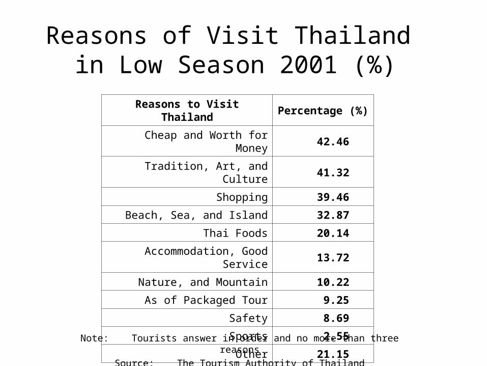
Reasons of Visit Thailand in Low Season 2001 (%)
Note: Tourists answer in order and no more than three reasons
Source: The Tourism Authority of Thailand
Reasons to Visit Thailand Percentage (%)
Cheap and Worth for Money 42.46
Tradition, Art, and Culture 41.32
Shopping 39.46
Beach, Sea, and Island 32.87
Thai Foods 20.14
Accommodation, Good Service 13.72
Nature, and Mountain 10.22
As of Packaged Tour 9.25
Safety 8.69
Sports 2.55
Other 21.15

Occupation of Tourists (%) 1996-2002
Note: Number of tourism excluding overseas Thai.
Source: The Tourism Authority of Thailand
Year
Occupation (percent, %)
Professionals Administrative
managerial Commercial personnel
Laborers, production
Other and not stated
1996 17 12 18 18 36
1997 19 13 17 15 37
1998 22 11 17 15 35
1999 19 11 17 18 35
2000 15 11 17 20 37
2001 15 11 17 19 39
2002 15 11 17 17 40

Tourist Consumption Expenditure 1996-2002
Note: Number of tourism excluding overseas Thai.
Source: The Tourism Authority of Thailand
Fig-2: Tourist consumption expenditure
219,364 220,754
242,177
253,018
200,000
210,000
220,000
230,000
240,000
250,000
260,000
1 2 3 4
Year (1=1996, 4=1999)
Mil
lio
n B
ah
t

Percentage Share of Tourist Expenditure 1996-2002
Note: Number of tourism excluding overseas Thai.
Source: The Tourism Authority of Thailand
Expenditure 1996 1997 1998 1999
Accommodation 20 25 27 24
Food and beverage 15 15 16 15
Sightseeing 6 6 4 4
Local transport 6 7 7 7
Shopping 38 34 29 35
Entertainment 10 10 11 11
Miscellaneous 5 3 5 4

Average Days of Stay in Thailand 1996-2002
Note: Number of tourism excluding overseas Thai.
Source: The Tourism Authority of Thailand
Year Average days of stay
1996 8.23
1997 8.33
1998 8.4
1999 7.96
2000 7.77
2001 7.96
2002 7.98

Quantity of Accommodations 1997-2001
Accommodations: Hotel, Guest House, Bangalore, Resort, Raft, Apartment, Motel
Source: The Tourism Authority of Thailand
Quantity of Accommodations
4762 4454 48375525 5701
0
2000
4000
6000
1 2 3 4 5
Year, 1= 1997, 5 = 2001
Quan
tity

The General Equilibrium Model
NATURE
PARK
LAND
RURAL TOURISM
AGRICULTURE
LABOR
URBAN TOURISM
MANUFACTURING
CAPITAL
RURAL AREA URBAN AREA
POLLUTION
EXPORT OR IMPORT

Summary of Notationr Rural tourism s Urban tourisma Agriculture m Manufacturexi Domestic demand
for good iyi Domestic supply
of good i pi Price of good i
L Labor endowmentK Capital endowment
l Land endowment, l =1T Land used in agriculturen Natural Park, (n+T=1)u Aggregate utility level z Pollution emitted from
manufacturing t Pollution taxt TariffMi Net import of tradable
good i

Summary of Functions
• Aggregate Expenditure Function
• Total Revenue Function
),,,,,,( uznppppE masr
}|{min uxpxpxpxp mmaassrrx
),,,,,,,( KLnppppG masr },|.{max KLzypypypyp mmaassrr
y

Aggregate Expenditure Function (1)
• Homogenous of degree one in all prices
• Concave in prices
• Non-decreasing in prices, utility, pollution emission, and natural park
),,,(),,,( uznpEuznpE
0,0 iii ppp EE
0,,, nzup EEEEi

Aggregate Expenditure Function (2)
• Shephard’s lemma, the demand for good i
• Output demand is downward sloping
• The shadow price of clean environment, or the marginal willingness for consumer to pay to for clean environment
0 ip xEi
0 iipp pxEii
0zE

Aggregate Expenditure Function (3)
• The shadow price of natural park, or the marginal willingness for consumer to pay to preserve natural park:
• Utility function
0nE
),,( znxuu
0,0,0 znx uuu

Total Revenue Function (1)
• Homogenous of degree one in all prices
• Homogenous of degree one in all factor endowments
),,,,(),,,,( KLnpGKLnpG
),,,,(),,,,( KLnpGKLnpG

Total Revenue Function (2)
• Convex in prices
• Concave in factor endowments
• The supply of good i
0,0 iii ppp GG
KLlvGG vvv ,,,0,0
0 ip yGi
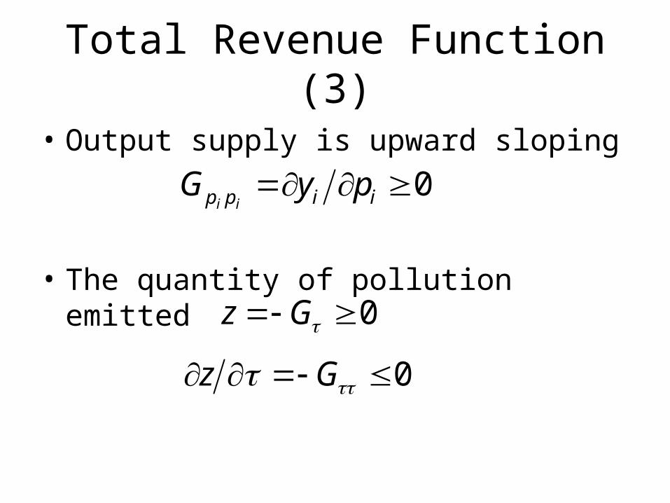
Total Revenue Function (3)
• Output supply is upward sloping
• The quantity of pollution emitted
0 iipp pyGii
0 Gz
0 Gz

Total Revenue Function (4)
• The wage of factor
• Factor demand is downward sloping
0 vwvG
0 vwG vvv
KLlv ,,

Equilibrium Conditions (1)
• The economy’s budget constrainttotal expenditure = total revenue
[1]
),,,,,,( uznppppE masr
),,,,,,,( KLnppppG masr z. i
iiMt

Equilibrium Conditions (2)
• Net import of tradable goods [2] to [5]
Good is imported if
Good is exported if
masri ,,,ii ppi GEM
,0iM
,0iM
0t
0t

Equilibrium Conditions (3)
• Pollution[6]
• Land market[7]
• Inverse world demand for rural tourism
[8]
• Inverse world demand for urban tourism
[9]
zG
1Tn
),),(,( znMpMpp ssrrr
),,),(( znMMppp srrss

Welfare Analysis (1)
• Exogenous variables
are given at world market prices
• Endogenous variables
are set by world demand for rural and
urban tourism
ma ppKL ,,,
masrsr MMMMunpp ,,,,,,,,
ma pp ,
sr pp ,

Welfare Analysis (2)
• Total differentiate [1], yield
• Rearrange and using [2] to [6], yield
[10]
duEdzEdnGEdpMdpM uznnssrr )()(
duEdzEdnEdpEdpE uznsprp sr
i
iii
iinsprp dtMdMtzddzdGdnGdpGdpGsr
i
iii
ii dtMdMt

Welfare Analysis (3)• Total differentiate [8], and rearrange, yield
[11]
[11’]
dzdz
dpdn
dn
dpdM
dM
dp
dp
dpdM
dM
dpdp rr
ss
s
s
rr
r
rr
rr
r
r
r
r
rr p
M
dM
p
M
dM
dpdp r
s
s
r
s
s
r pM
dM
p
M
dM
dp
rr
r pn
dn
p
n
dn
dpr
r
r pz
dz
p
z
dz
dp
zpnpMpMpdp rrrrsrsrrrrr ˆˆˆˆ
znMMp rrssrrrr ˆˆˆˆˆ

Welfare Analysis (4)
• Similarly, total differentiate [9], yield
[12]
[12’]
• Where, for Proportional change of tourism prices
Proportional change of tourism import
zpnpMpMpdp sssssssrsrss ˆˆˆˆ
znMMp ssssrrss ˆˆˆˆˆ
iii pdpp ˆ
iii MdMM ˆ
sri ,

Welfare Analysis (5)Own inverse elasticity of world
demand for tourism
Cross inverse elasticity of world demand for tourism
Inverse elasticity of Natural Park to tourism prices
Inverse elasticity of pollution to tourism prices
j
i
i
jij p
M
dM
dp
i
ii p
n
dn
dp
i
ii p
z
dz
dp
srji ,, ji
i
i
i
ii p
M
dM
dp

Welfare Analysis (6)
• Substitute [11] and [12] in [10] and rearrange, yield
[13]
uuEu ˆ rssrsrrrrr MMpMpMt ˆ)(
aaa MMt ˆ mmm MMt ˆ
nppnEnG ssrrnn ˆ)(
i
iii tMt ˆ
ssssrrsrss MMpMpMt ˆ)(
zppzEz zzrrz ˆ).(

Tourism Promotion Policy (1)
• I would like to analyze the effects of “tourism promotion policy” on the social welfare.
• The tourism promotion policy indicates the increases in
rural tourism export and/or urban tourism export, i.e.
• For simplicity and isolation of the problem, I assume that there are no tariffs, i.e. free trade policy in all sectors.
• Therefore, the welfare effects equation is reduced to [13A] below:
0ˆ,ˆ sr MM
0it masri ,,,
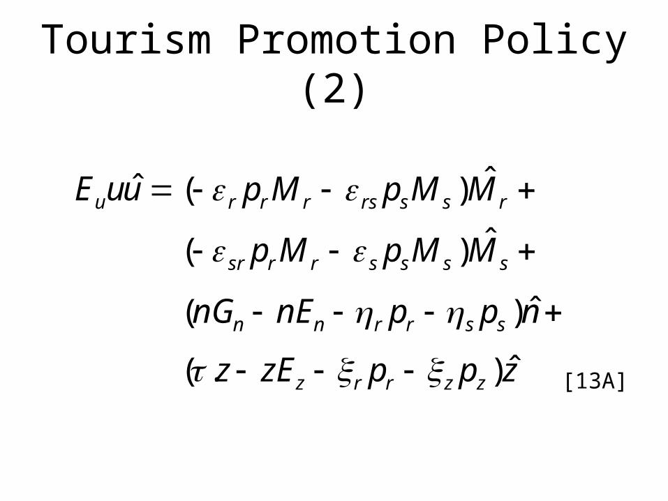
Tourism Promotion Policy (2)
[13A]
ssssrrsr MMpMp ˆ)(
uuEu ˆ rssrsrrr MMpMp ˆ)(
nppnEnG ssrrnn ˆ)(
zppzEz zzrrz ˆ).(

The Sign (1)• If both rural and urban tourism are normal goods with inelastic
demand, then
• If both rural and urban tourism are normal goods with elastic demand, then
• If rural and urban tourism are substitutes, then
• If rural and urban tourism are complements, then
1,0 sr
1, sr
0, srrs
0, srrs

The Sign (2)
• As mentioned before, this is the shadow price of clean environment (the marginal willingness for consumer to pay for clean environment)
• As mentioned before, this is the shadow price of natural
park (the marginal willingness for consumer to pay to preserve natural park)
0zE
0nE
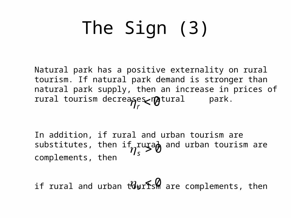
The Sign (3)
Natural park has a positive externality on rural tourism. If natural park demand is stronger than natural park supply, then an increase in prices of rural tourism decreases natural park.
In addition, if rural and urban tourism are substitutes, then if rural
and urban tourism are complements, then
if rural and urban tourism are complements, then
0r
0s
0s

The Sign (4)
If natural park supply is stronger than natural park demand, then an
increase in prices of rural tourism increases natural park
In addition, if rural and urban tourism are substitutes, then if rural
and urban tourism are complements, then
if rural and urban tourism are complements, then
0r
0s
0s

The Sign (5)
Pollution has a negative externality on urban tourism. If urban tourism demand is stronger than urban tourism supply, then an increase in pollution decreases urban tourism demand, and so
decreases prices of urban tourism.
In addition, if rural and urban tourism are substitutes, then if rural
and urban tourism are complements, then
if rural and urban tourism are complements, then
0s
0r
0r

Example of Policy Implication (1)
Example 1: • Fixed agricultural land and natural park policy: • Fixed pollution emission policy: • Rural and urban tourism promotion:
Then:
• If rural and urban are complements, then there is a welfare improvement.
• If rural and urban are substitutes, then welfare effects are ambiguous.
nnTT ,zz
uuEu ˆ
,0, sr MM 0ˆ,ˆ sr MM
ssssrrsrrssrsrrr MMpMpMMpMp ˆ)(ˆ)(

Example of Policy Implication (2)
Example 2: • Rural and urban tourism promotion:
Then:
• If rural and urban are complements, and there is a perfect property right or tax system on both natural park and pollution so that:
• So there is a welfare improvement. And the optimal shadow price of natural park, and the optimal pollution tax are:
uuEu ˆ
,0, sr MM 0ˆ,ˆ sr MM
ssssrrsrrssrsrrr MMpMpMMpMp ˆ)(ˆ)( zppzEznppnEnG zzrrzssrrnn ˆ).(ˆ)(
0 ssrrnn ppnEnG 0. zzrrz ppzEz
n
ppnGE ssrrnn
z
ppzE ssrrz

Example of Policy Implication (3)
Example 3: • Fixed pollution emission policy: • Rural and urban tourism promotion: • Increase natural park:
Then:
• If rural and urban are complements, then an increase in natural park ambiguously improve welfare if
• Note: If people do not care about natural park, , then an increase in natural park ambiguously improve welfare if
zz
uuEu ˆ
,0, sr MM 0ˆ,ˆ sr MM
ssssrrsrrssrsrrr MMpMpMMpMp ˆ)(ˆ)(
0ˆ n
nppnEnG ssrrnn ˆ)(
ssrrnn ppnGnE
0nE
0, sr

Example of Policy Implication (4)
Example 4: • Fixed agricultural land and natural park policy: • Rural and urban tourism promotion: • Decrease pollution:Then:
• If rural and urban are complements, then a decrease in pollution ambiguously improve welfare if
uuEu ˆ
,0, sr MM 0ˆ,ˆ sr MM
ssssrrsrrssrsrrr MMpMpMMpMp ˆ)(ˆ)(
0ˆ z
nnTT ,
zppzEz zzrrz ˆ).(
zzrrz ppzzE .

Other Results
• There are many other implication results which could be drawn from the welfare equation [13]. These results are left for further exercises.
• Further research is also needed in order to determine the own price and cross price elasticities as well as other elasticities for the amenity such as natural park and pollution.