AADE-07-NTCE-53 API RP 13C D100 Values, Split Curves, and Separation Efficiency

Copyright 2007, AADE This paper was prepared for presentation at the 2007 AADE National Technical Conference and Exhibition held at the Wyndam Greenspoint Hotel, Houston, Texas, April 10-12, 2007. This conference was sponsored by the American Association of Drilling Engineers. The information presented in this paper does not reflect any position, claim or endorsement made or implied by the American Association of Drilling Engineers, their officers or members. Questions concerning the content of this paper should be directed to the individuals listed as author(s) of this work.

Abstract

The API RP 13C laboratory procedure for measuring screen D100 values is a step forward for the drilling industry. The D100 value estimates the diameter of the coarsest particles that pass through a screen cloth sample. The procedure uses screen samples and precise amounts of grits of known sizes, both coarser and finer than the anticipated screen sample, within a stack of standard ASTM sieves. After the stack is shaken, the resulting distribution of dry grit determines the D100 value.

In a separate set of tests, separation performance has also been measured in a pilot plant using drilling fluid and a full size shale shaker. The pilot plant fluid included a controlled distribution of sand particles to represent the drill cuttings. The particle size distribution and rheological properties were held as constant as possible while the fluid was pumped in circulation through the shaker. Samples were collected and material balances were calculated covering all particle size fractions and the liquid split. Next, Split Curves were prepared. The Split Curve, also known as the partition curve or the Cut Point Curve, is a useful graphic presentation of particle size separations. It shows the percent of the particles of each size that report to the discard or oversize stream of a separating device. The pilot plant data shows a good correlation between the D100 values obtained from the laboratory API RP 13C procedure and the equivalent values taken from the Split Curve data.

Relationships between the Split Curves and separation efficiency values are also illustrated. Several aspects of separation efficiency are shown graphically within a Split Curve, including misplaced coarse particles, misplaced fine particles, and the overall efficiency value. These efficiency values are then calculated from the pilot plant data. Introduction

In support of the new API RP 13C procedure, screen manufacturers have been measuring and publishing the D100 values of their screen products. The API RP 13C D100 procedure is the latest in a series of API Recommended Practices designed to provide a reproducible and reliable measure of particle size separations made by screen cloth. The procedure is written in such specific language that very similar D100 values should be obtained for any given cloth combination, no matter when or where a test is run.

As a laboratory procedure however, the D100 value was

not originally intended to reflect the entire complexity of screen separation performance on a full scale shaker. Instead, it provides rig operators with a common designation for screen selection and screen comparison tests.

At about the same time that API RP 13C work was in full swing at Brandt NOV, a pilot plant test campaign was started to better understand shaker performance under operating conditions similar to field conditions, and using as many screen sizes as possible. After the test sequence was completed, the samples measured, and the data compiled, a relationship was found between the API RP 13C D100 values and the equivalent values taken from the pilot plant Split Curve. In addition to this relationship, the Split Curve also was used to visualize several measures of separation efficiency.

In this study, Split Curves were found to be a useful conceptual link between full scale pilot plant screen separation performance, laboratory D100 values, and separation efficiency values. The purpose of this paper is to describe relationships between these three concepts, in order to distinguish how they are different, but related. The detailed API RP 13C D100 procedure can be found elsewhere1 and need not be described again here. This paper will describe pilot plant test procedures first and the derivation of Split Curves from pilot plant data will follow. The determination of a pilot plant Split Curve measurement as an equivalent to the laboratory RP 13C D100 value is then shown, and finally Split Curves are used to explain three separation efficiency terms, along with two additional values relating to the quality of the separation. Pilot Plant Tests

The pilot plant tests used a Brandt NOV King Cobra full scale shaker fitted with three operating screens and a drying screen. The shaker was mounted above a mud tank so that the shaker discard stream was allowed to return by gravity through the top of the tank and back into the fluid. The shaker itself was mounted in an elevated position to facilitate collecting underflow samples. All of the undersize material from the shaker was collected into one steel trough located under the shaker. The trough carries the total underflow stream out from under the shaker and empties into the mud tank in a position that allows accurate samples to be taken as the fluid falls into the tank. Finally, a centrifugal pump returned the mixed fluid back into the shaker feed box, so that

AADE-07-NTCE-53

API RP 13C D100 Values, Split Curves, and Separation Efficiency Thomas R. Larson, Brandt NOV

2 Thomas R. Larson AADE-07-NTCE-53

the entire system was recirculating during each test run. Figure 1 shows the general orientation of the equipment. An agitator in the mud tank ran continuously, keeping the fluid in suspension.

Feed Particle Size Control

To maintain the feed size distribution over a long series of tests, a particle size degradation rate measurement was completed before the first split test. The degradation rate test measures the rate in which the particle size distribution changes over a known time span. Two areas are of concern; the coarse end of the size distribution is milled by the action of the centrifugal pump and by turbulence caused by every tee or elbow in the feed pipeline downstream of the pump. The fine end of the size distribution grows at the same rate the coarse end is milled. If the particle size is to be held constant, these changes need to be minimized and accommodated.

The degradation rate test starts by running the entire circulating system using the actual conditions relevant during the split tests, including through the shaker fitted with screens. Two feed samples are collected: one initially, and one after a measured run time of 4 hours. The difference in the particle size distributions over that time span is used to measure the rate of change of the particle sizes, by particle size. From this data, an addition rate and a specific blend of sized particles is found that eliminates the coarse end change. That addition rate of specifically sized particles is used for the duration of the subsequent test sequence.

In this particular example, the first degradation rate test revealed the need for adjustments to the feed pipeline. After the adjustments were complete, a second degradation rate test measured a new reduced rate of coarse particle degradation. Thankfully, the final addition rate of coarse particles was measured in pounds per hour rather than tons per hour.

Fluid Rheological Control

During the test campaign, fluid rheology is monitored using the following schedule of tests:

Every Hour: Pilot Plant staff: • Funnel Viscosity • Sand Content • Temperature Measurements • Samples collected for the Analytical Lab:

Every Hour: Analytical Lab staff: • Particle size distribution analysis

Every Other Hour: Analytical Lab staff: • PV, YP, and gel strength from a Fann viscosimeter, • Active clay content by the Methylene Blue Test.

During the campaign, the pilot plant staff remains in regular communication with the Analytical Laboratory staff, and both have the training and authority to adjust any addition rate or related procedure that might be required to hold the mud properties as constant as possible.

While maintaining the coarse particle size distribution constant, colloidal sized particles are also created at the same rate as the addition of coarse sand. They need to be removed

at a rate that prevents them from building up enough to impact fluid viscosity. The removal of the finest particles can be done with a pilot scale centrifuge, but in this test campaign a screen rinsing step accomplished the same purpose, as described in the following section.

Pilot Plant Test Procedure

A typical test day begins with a short time of circulating the mud through the equipment to rinse down, flush out, and re-mix any material that may have settled or dried into place overnight. Next, the selected test screens are installed, and the feed flow rate is adjusted to provide the desired beach position on the shaker screens. Sufficient run time is then allowed to greatly exceed three retention times before sampling begins. Next, the discard stream flow rate is measured three times. Figure 2 shows the tool specifically designed for this purpose, called the discard cutter. The discard cutter is placed to catch the entire shaker discard stream three times, and each fill event is timed and the collected material weighed before it is returned back into the mud tank.

Samples are then collected for performance analysis. Each sample is collected using specifically designed hardware. Feed samples are collected from a small bypass hose attached to a vertical run of the feed pipe. Underflow samples are collected by swinging an underflow sample cutter, shown in Figure 3, through the flow exiting the underflow collection trough, and the discard samples are collected with the same cutter used to measure the discard flow rate. The discard cutter has the capacity to collect 100 percent of the expected flow for about 3 to 10 minutes duration, depending on loading. When sampling, of course, the collected material is emptied into a sample container instead of returning it to the sump.

After sampling is complete, the feed stream is bypassed out of the shaker and though a tank of known volume which then discharges into the mud tank. Periodically, it is possible to measure the feed flow rate directly, because the known volume tank can be sealed off with a manually operated plug, and the rise rate of the fluid in the tank can be recorded.

The screens are then removed from the shaker and are rinsed carefully, both to recover and return the coarse particles to the tank, but also to remove the colloidal particles. Each screen is placed individually in the discard sample cutter during the rinse step. After the screen is clean, the liquid collected in the cutter is discarded into an adjacent storage tank, but the coarse sand that settled into the bottom of the cutter is returned to the mud tank. In this way, a volume of colloidal particles are carried with the discarded fluid out of the system every time a screen is rinsed, but the rinsing step does not increase the disappearance rate of coarse particles. This screen rinsing method removed sufficient amounts of colloidal particles to avoid impacting the fluid rheology.

Conversion of Data into Information

Material Balance Example Calculations

Particle size distributions were measured on all samples, using a proprietary sequence that includes wet sieving, dry

AADE-07-NTCE-53 Thomas R. Larson 3

sieving, and a Microtrac 3500 Particle Size Analyzer. Table 1 shows an example set of measured size structures. After each set of particle size distribution measurements were complete, the measured size data was used to calculate material balances for each separation. Balanced size values are necessary for determining the correct recovery and distribution values in any separation process. If measured, but unbalanced data is used for determining separation performance, small but normally present measurement variations produce calculation errors that appear to create or destroy matter. Unfortunately, recovery values calculated this way not only cannot be correct, but they are may not be obviously wrong. All separation performance and Split Curve data in this paper were calculated from material balances calculated from particle size data, measured from samples collected in as representative a way as possible, from machinery operating as close to equilibrium as possible. In addition, each material balance was also used to measure the quality of the unbalanced data.

The measured data used for this example is presented in the left hand set of columns in Table 1. To calculate the material balance, the following algebra is used, starting with two conservation of mass relationships:

F = U + D (1)

fiF = uiU + diD (2)

where: F is the unknown total mass flow of feed, fi are the measured feed size distribution data, U is the unknown undersize total mass flow, ui are the measured undersize size distribution data, D is the measured discard total mass flow, and di are the measured discard size distribution data. In this example, only the size fraction data is known,

together with a physical measurement of the discard stream bulk flow rate D. For the general case, these equations are re-arranged to isolate the ratio of U/D in terms of the known values of fi, ui, and di from sample data, as follows:

fi(U + D) = uiU + diD (3)

fiU + fiD = uiU + diD (4)

fiD - diD = uiU - fiU (5)

(fi - di)*D = U*(ui - fi) (6)

(fi - di) = (U / D)*(ui - fi) (7)

If (fi - di) is plotted on the y-axis and (ui - fi) is plotted on

the x-axis, then the slope of the resulting line equals (U / D),

which is the ratio of the underflow mass flow over the discard mass flow. If all size fractions are plotted on the same graph, all of the points should generally arrange themselves in a straight line following the Y = mX + b format. However, note that equation (7) must pass through the origin, and so b=0.

If the size distribution measurements and sampling were done perfectly, the feed, underflow, and discard stream size fraction values have to reflect the same bulk material split behavior for each size fraction, leaving only one value for the ratio of (U / D). In the perfect case, each point would have the same slope with respect to the origin, and therefore all of the data points align on one straight line.

Sampling and analysis variations results in points that spread a bit, unfortunately, but the true weight split value will be the slope of the best straight line through all of the data. Linear regression can be used to determine the best value of the coefficient “m” from the Y = mX formula. Figure 4 shows this chart produced from the example data in Table 1.

The R2 value for the regression equation can also be calculated. This value relates inversely to the total variation in the data, spanning from 0 (completely random) to 1 (perfectly straight). Therefore, the value of R2 can be considered a measure of the perfection achieved by the raw data, related as a percent. If the data produces a very widely dispersed set of points, the dispersion is quantified by a low value for R2. At some arbitrarily low value, the best option may be to throw out the samples and repeat the test.

In contrast, a high value of R2 means that the raw data are all in agreement over the slope of the line because the accumulated error from sample collection, sample processing, and measurement is very small. In Figure 4, the raw data points are shown for the material balance example, and the solid line is the trend line with the best slope, shown here with the R2 value. This method provides a valuable data quality measure that is not achieved by using unbalanced data.

After the slope is known, it can be used to calculate the bulk weight split, determined as a percent of the feed by replacing F in equation (1) with the value 1 (100%).

D = F – U = 1 – U (8)

U / D = m (9)

U / (1 – U) = m (10)

U = m – U * m (11)

U + U * m = m (12)

U * (1 + m) = m (13)

U = m / (1 + m) (14)

where:

m is the slope of the trend line from Figure 4


Once the weight split is known, standard methods to determine the balanced individual size fraction values with minimum error can be used. The balanced values for the example data set are also shown in Table 1.

Split Curve Description

After material balances are complete, a number of additional calculations can be made. One graphic presentation of particle size separations is the Split Curve, also known as the partition curve or the Cut Point Curve. The Split Curve is simply a graph showing the percent of the particles of each size that report to the discard or oversize stream of a separating device. Particle size is plotted along the x-axis, while the 0 to 100% value, plotted on the y-axis, in this case represents the fraction of each particle size that reports to the discard of the shaker.

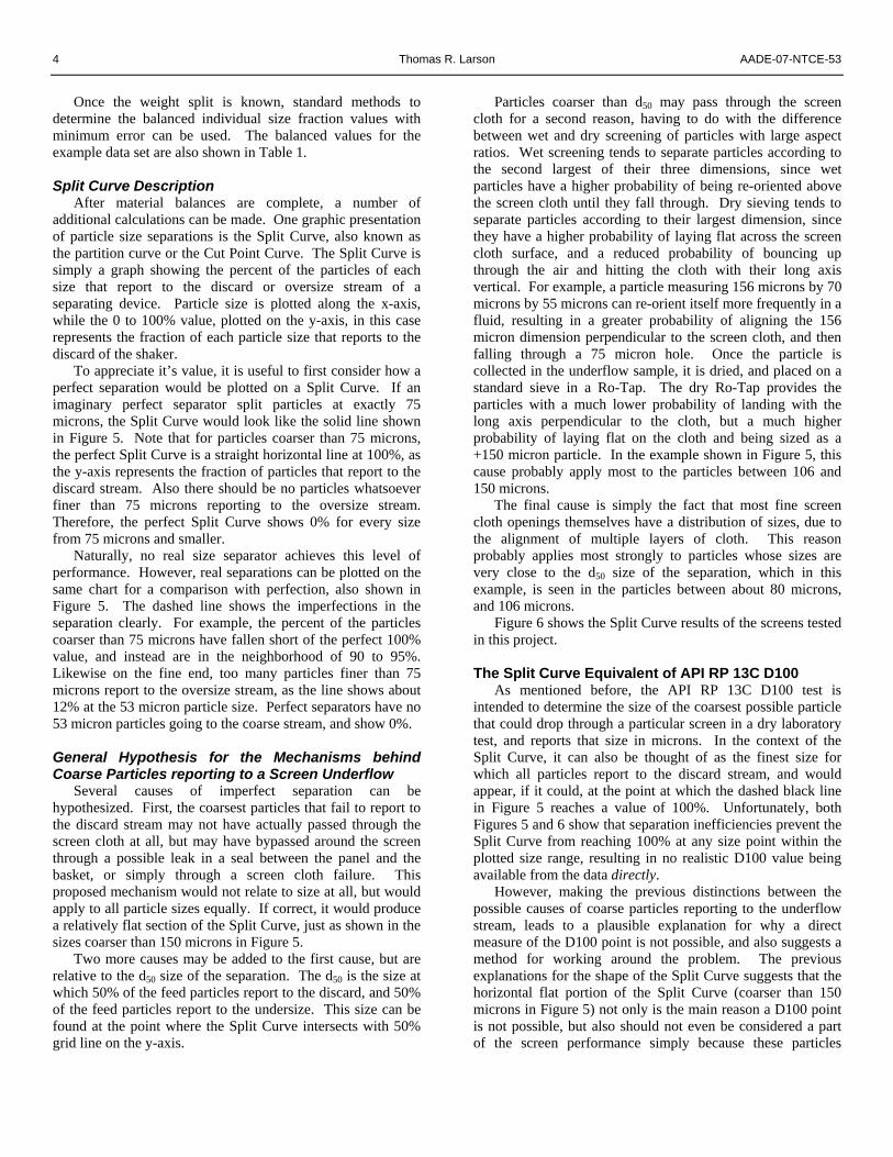
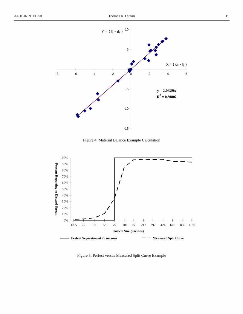
To appreciate it’s value, it is useful to first consider how a perfect separation would be plotted on a Split Curve. If an imaginary perfect separator split particles at exactly 75 microns, the Split Curve would look like the solid line shown in Figure 5. Note that for particles coarser than 75 microns, the perfect Split Curve is a straight horizontal line at 100%, as the y-axis represents the fraction of particles that report to the discard stream. Also there should be no particles whatsoever finer than 75 microns reporting to the oversize stream. Therefore, the perfect Split Curve shows 0% for every size from 75 microns and smaller.

Naturally, no real size separator achieves this level of performance. However, real separations can be plotted on the same chart for a comparison with perfection, also shown in Figure 5. The dashed line shows the imperfections in the separation clearly. For example, the percent of the particles coarser than 75 microns have fallen short of the perfect 100% value, and instead are in the neighborhood of 90 to 95%. Likewise on the fine end, too many particles finer than 75 microns report to the oversize stream, as the line shows about 12% at the 53 micron particle size. Perfect separators have no 53 micron particles going to the coarse stream, and show 0%.

General Hypothesis for the Mechanisms behind Coarse Particles reporting to a Screen Underflow

Several causes of imperfect separation can be hypothesized. First, the coarsest particles that fail to report to the discard stream may not have actually passed through the screen cloth at all, but may have bypassed around the screen through a possible leak in a seal between the panel and the basket, or simply through a screen cloth failure. This proposed mechanism would not relate to size at all, but would apply to all particle sizes equally. If correct, it would produce a relatively flat section of the Split Curve, just as shown in the sizes coarser than 150 microns in Figure 5.

Two more causes may be added to the first cause, but are relative to the d50 size of the separation. The d50 is the size at which 50% of the feed particles report to the discard, and 50% of the feed particles report to the undersize. This size can be found at the point where the Split Curve intersects with 50% grid line on the y-axis.

Particles coarser than d50 may pass through the screen cloth for a second reason, having to do with the difference between wet and dry screening of particles with large aspect ratios. Wet screening tends to separate particles according to the second largest of their three dimensions, since wet particles have a higher probability of being re-oriented above the screen cloth until they fall through. Dry sieving tends to separate particles according to their largest dimension, since they have a higher probability of laying flat across the screen cloth surface, and a reduced probability of bouncing up through the air and hitting the cloth with their long axis vertical. For example, a particle measuring 156 microns by 70 microns by 55 microns can re-orient itself more frequently in a fluid, resulting in a greater probability of aligning the 156 micron dimension perpendicular to the screen cloth, and then falling through a 75 micron hole. Once the particle is collected in the underflow sample, it is dried, and placed on a standard sieve in a Ro-Tap. The dry Ro-Tap provides the particles with a much lower probability of landing with the long axis perpendicular to the cloth, but a much higher probability of laying flat on the cloth and being sized as a +150 micron particle. In the example shown in Figure 5, this cause probably apply most to the particles between 106 and 150 microns.

The final cause is simply the fact that most fine screen cloth openings themselves have a distribution of sizes, due to the alignment of multiple layers of cloth. This reason probably applies most strongly to particles whose sizes are very close to the d50 size of the separation, which in this example, is seen in the particles between about 80 microns, and 106 microns.

Figure 6 shows the Split Curve results of the screens tested in this project.

The Split Curve Equivalent of API RP 13C D100

As mentioned before, the API RP 13C D100 test is intended to determine the size of the coarsest possible particle that could drop through a particular screen in a dry laboratory test, and reports that size in microns. In the context of the Split Curve, it can also be thought of as the finest size for which all particles report to the discard stream, and would appear, if it could, at the point at which the dashed black line in Figure 5 reaches a value of 100%. Unfortunately, both Figures 5 and 6 show that separation inefficiencies prevent the Split Curve from reaching 100% at any size point within the plotted size range, resulting in no realistic D100 value being available from the data directly.

However, making the previous distinctions between the possible causes of coarse particles reporting to the underflow stream, leads to a plausible explanation for why a direct measure of the D100 point is not possible, and also suggests a method for working around the problem. The previous explanations for the shape of the Split Curve suggests that the horizontal flat portion of the Split Curve (coarser than 150 microns in Figure 5) not only is the main reason a D100 point is not possible, but also should not even be considered a part of the screen performance simply because these particles


probably did not go through the screen cloth at all. On the other hand, the sloped portion of the Split Curve probably relates to particles that have gone through the cloth, and therefore is an important part of the separation performance of the cloth.

Therefore, the best method of estimating an equivalent D100 value is to introduce two more Split Curve based values: the d25 and the d75 sizes. Just as their name implies, these points are the size values at which 25% of the particles report to the discard stream, and at which 75% of the particles report to the discard stream, respectively. A Split Curve based equivalent of the laboratory D100 value can be determined by extrapolating the d25 and d75 points on the Split Curve up to the 100 percent gridline, and recording the size of the intersection point. This procedure essentially ignores the fact that the coarse end of the Split Curve becomes a horizontal line at a value less than 100% (for sizes coarser than 150 microns in Figure 5), just as it should if those particles never really went through the screen cloth. It does, however, include the effect of particles near the d50 size that probably have gone through the cloth due to either previous explanation. Figure 7 illustrates this solution to the problem of finding an equivalent D100 value from pilot plant data. In order to distinguish this value from the laboratory based API RP 13C D100 number, it is labeled Split-100.

Using Split-100 values, it is now possible to compare the same D100 concept extracted from pilot plant data against the API RP 13C D100 values determined according to the laboratory procedure. Since all of the screens used in the test sequence have also been measured using the API RP 13C procedure, this comparison is made and shown in Table 2 and plotted in Figure 8. Figure 8 also contains a solid line graphically indicating where the two would be equal, and a dotted line that is the trend line calculated from the points themselves. The slope of the trend line in Figure 8 reveals that there is also a constant but small offset of 5½% between the two measurements. The correlation between these two values is relatively good, at R2 = 0.9062, which supports the idea that the API RP 13C D100 procedure provides a good estimate of pilot plant separation performance, even though it is a dry bench scale separation. In other words, if it were stated that Split-100 values were simply 5½% coarser than the API D100 values for the tested screens, it would be a correct statement more than 90% of the time.

Split Curves and Separation Efficiency

Split Curves can also be used to show separation efficiency. Figure 9 repeats Figure 5, with the addition areas highlighted for emphasis. Figure 9 shows that a substantial area of particles coarser than 75 microns is successfully reporting to the coarse stream. These particles can be called “Perfectly Split Coarse”, since they went where they were supposed to go. A similar area can be identified for fine particles. However, perfectly split fine particles are represented by the area above the dashed line, not below, because these particles should not report to the oversize stream. These areas are colored green (or lightly shaded) in

Figure 9 on the lower right and upper left hand sides respectively.

In the opposite sense, the areas of Figure 9 not highlighted in green represents coarse particles that do not report to the oversize stream but should, on the upper right, and fine particles that do report to the oversize stream, but shouldn’t, on the lower left. Because of this, these areas represent “misplaced coarse” and “misplaced fine” particles, respectively, and are highlighted in red (or shaded darkly) in Figure 9.

Overall separation efficiency can now be described as that portion of all particles that actually did report to the stream to which they were intended to go. From Figure 9, it is simply the sum of the green areas divided by the total area shown in the chart. Several other useful concepts can be observed as well. The undersize efficiency would simply be the ratio of the green area on the left of the 75 micron line, divided by the total area to the left of the 75 micron line. Likewise the oversize efficiency is the same ratio of the areas to the right of the 75 micron line. Conceptually, these are accurate descriptions, but they are not quantitative.

Quantifying Separation Efficiency

In order to quantify efficiency, an important limitation regarding Split Curves should be noted: The overall feed particle size distribution is not indicated by the Split Curve in any way, because the y-axis shows only the percent of the feed particles of each size category that report to the discard stream. This means that the Split Curve is insensitive to slight changes in the feed size distributions from test to test. However, the plotted values provide no reference to the weight in that size fraction relative to the weights in the other size fractions. Therefore, the areas of Figure 9 cannot quantify the efficiency of the separation, but only provide a relative indication of efficiency. Of the entire plotted area shown in Figure 9, the more green area there is (or the less red area), the higher the efficiency. Split Curves alone are useful for estimating separation efficiencies only when there are several tests in a series with feed size distributions as constant as possible, or when a series of shakers are fed from a common source.

In 1970, N.F. Schulz published a review article2 on separation efficiency applied to the mining industry. The Schulz method is applicable to any particle size based separation, and also incorporates feed size distribution values, such that the resulting efficiencies values themselves are independent of feed size variations. Applied to shakers, one minor modification is required. The Schulz paper includes the separations of minerals that are not completely liberated from one another. This complexity is not necessary when dealing with size distributions, because by definition each size fraction is perfectly liberated from every other size fraction. Figure 10 shows an example of this calculation, described as follows.

To evaluate the separation performance of any machine designed to separate particles by size, the distinction between coarse and fine particles must be made first. In this paper, the size that divides coarse from fine particles is called the Size of


Reference, and in the examples and figures so far, it has been selected as 75 microns. This value for Size of Reference was chosen first because it is an important part of the API criteria for barite particle size, and second because there is a standard sieve produced at that size, making it very practical when using standard laboratory sieves.

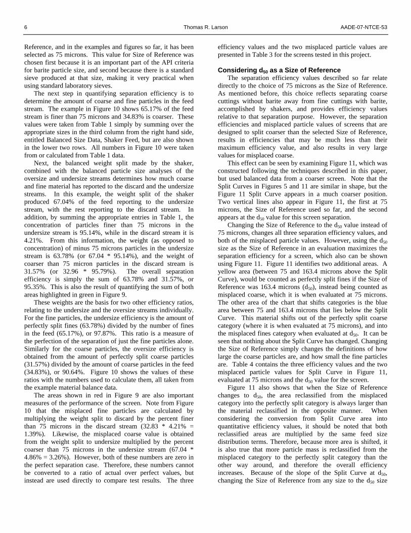
The next step in quantifying separation efficiency is to determine the amount of coarse and fine particles in the feed stream. The example in Figure 10 shows 65.17% of the feed stream is finer than 75 microns and 34.83% is coarser. These values were taken from Table 1 simply by summing over the appropriate sizes in the third column from the right hand side, entitled Balanced Size Data, Shaker Feed, but are also shown in the lower two rows. All numbers in Figure 10 were taken from or calculated from Table 1 data.

Next, the balanced weight split made by the shaker, combined with the balanced particle size analyses of the oversize and undersize streams determines how much coarse and fine material has reported to the discard and the undersize streams. In this example, the weight split of the shaker produced 67.04% of the feed reporting to the undersize stream, with the rest reporting to the discard stream. In addition, by summing the appropriate entries in Table 1, the concentration of particles finer than 75 microns in the undersize stream is 95.14%, while in the discard stream it is 4.21%. From this information, the weight (as opposed to concentration) of minus 75 microns particles in the undersize stream is 63.78% (or 67.04 * 95.14%), and the weight of coarser than 75 micron particles in the discard stream is 31.57% (or 32.96 * 95.79%). The overall separation efficiency is simply the sum of 63.78% and 31.57%, or 95.35%. This is also the result of quantifying the sum of both areas highlighted in green in Figure 9.

These weights are the basis for two other efficiency ratios, relating to the undersize and the oversize streams individually. For the fine particles, the undersize efficiency is the amount of perfectly split fines (63.78%) divided by the number of fines in the feed (65.17%), or 97.87%. This ratio is a measure of the perfection of the separation of just the fine particles alone. Similarly for the coarse particles, the oversize efficiency is obtained from the amount of perfectly split coarse particles (31.57%) divided by the amount of coarse particles in the feed (34.83%), or 90.64%. Figure 10 shows the values of these ratios with the numbers used to calculate them, all taken from the example material balance data.

The areas shown in red in Figure 9 are also important measures of the performance of the screen. Note from Figure 10 that the misplaced fine particles are calculated by multiplying the weight split to discard by the percent finer than 75 microns in the discard stream (32.83 * 4.21% = 1.39%). Likewise, the misplaced coarse value is obtained from the weight split to undersize multiplied by the percent coarser than 75 microns in the undersize stream (67.04 * 4.86% = 3.26%). However, both of these numbers are zero in the perfect separation case. Therefore, these numbers cannot be converted to a ratio of actual over perfect values, but instead are used directly to compare test results. The three

efficiency values and the two misplaced particle values are presented in Table 3 for the screens tested in this project. Considering d50 as a Size of Reference

The separation efficiency values described so far relate directly to the choice of 75 microns as the Size of Reference. As mentioned before, this choice reflects separating coarse cuttings without barite away from fine cuttings with barite, accomplished by shakers, and provides efficiency values relative to that separation purpose. However, the separation efficiencies and misplaced particle values of screens that are designed to split coarser than the selected Size of Reference, results in efficiencies that may be much less than their maximum efficiency value, and also results in very large values for misplaced coarse.

This effect can be seen by examining Figure 11, which was constructed following the techniques described in this paper, but used balanced data from a coarser screen. Note that the Split Curves in Figures 5 and 11 are similar in shape, but the Figure 11 Split Curve appears in a much coarser position. Two vertical lines also appear in Figure 11, the first at 75 microns, the Size of Reference used so far, and the second appears at the d50 value for this screen separation.

Changing the Size of Reference to the d50 value instead of 75 microns, changes all three separation efficiency values, and both of the misplaced particle values. However, using the d50 size as the Size of Reference in an evaluation maximizes the separation efficiency for a screen, which also can be shown using Figure 11. Figure 11 identifies two additional areas. A yellow area (between 75 and 163.4 microns above the Split Curve), would be counted as perfectly split fines if the Size of Reference was 163.4 microns (d50), instead being counted as misplaced coarse, which it is when evaluated at 75 microns. The other area of the chart that shifts categories is the blue area between 75 and 163.4 microns that lies below the Split Curve. This material shifts out of the perfectly split coarse category (where it is when evaluated at 75 microns), and into the misplaced fines category when evaluated at d50. It can be seen that nothing about the Split Curve has changed. Changing the Size of Reference simply changes the definitions of how large the coarse particles are, and how small the fine particles are. Table 4 contains the three efficiency values and the two misplaced particle values for Split Curve in Figure 11, evaluated at 75 microns and the d50 value for the screen.

Figure 11 also shows that when the Size of Reference changes to d50, the area reclassified from the misplaced category into the perfectly split category is always larger than the material reclassified in the opposite manner. When considering the conversion from Split Curve area into quantitative efficiency values, it should be noted that both reclassified areas are multiplied by the same feed size distribution terms. Therefore, because more area is shifted, it is also true that more particle mass is reclassified from the misplaced category to the perfectly split category than the other way around, and therefore the overall efficiency increases. Because of the slope of the Split Curve at d50, changing the Size of Reference from any size to the d50 size


causes a similar pair of category switches, but the area reclassified as perfectly split is always larger than the area reclassified as misplaced. Therefore, defining particles as coarse and fine according to the d50 point always results in maximum overall separation efficiency.

Efficiency values based on d50 as the Size of Reference should be thought of as normalized by the screens cut points. Normalized efficiency values are not influenced by the distance between d50 and an arbitrary Size of Reference. The efficiency differences between screens in this case, therefore, are also independent of the Size of Reference, and require a slightly different interpretation.

In contrast, efficiencies evaluated at a constant Size of Reference ranks the screens as to their value in terms of making a cut at the specific Size of Reference. If the use of barite demands an efficiency evaluation at 75 microns, then the constant Size of Reference is at 75 microns is the proper way to compare efficiencies. Both options have value, they simply have two different purposes.

Conclusions

In conclusion, several relationships between screen performance measurements, and their limitations, can now be observed: 1) API RP 13C D100 values, based on dry separations in the

laboratory, are shown here to correlate well with the equivalent value derived from Split Curves measured from a full scale shaker processing drilling fluid. In this data set, the pilot plant equivalent value is approximately 5½ percent coarser than the API RP 13C data, and correlates with an R2 value over 90%.

2) The concept of the Size of Reference has been introduced as a necessary specification when referring to separation efficiency. Separation efficiency values are completely meaningless without specifying their Size of Reference.

3) The Split Curve not only presents a graphic image of separation performance, but when a vertical line is added at the Size of Reference, three separation efficiency values, and two misplaced particle values can also be graphically represented. The graph area becomes divided into two areas representing Perfectly Split particles, and two areas representing misplaced particles, and forms an easily visualized performance measurement.

4) Split Curves must be constructed from data that has been through a material balance calculation. If not, undetected but normal variations in sample collection, sample handling, and size distribution measurements may falsely lead to recovery values based on either created or destroyed matter. A simple method has been presented for determining the total accumulated error of the measured data that can be used to prevent conclusions from being drawn from poor data. The example data set in this paper shows good measured data accuracy, shown in Figure 4 with an R2 value better than 98%.

5) The graphic representation of separation efficiency within a Split Curve can be converted to quantitative efficiency values, using the balanced feed, discard, and underflow

size distributions and the selected Size of Reference, following calculation described by N. F. Schulz.

6) Quantifying efficiencies from Split Curves depends on the value chosen as the Size of Reference. One choice over another is neither better nor worse, but simply requires different interpretations. a. The 75 micron choice reflects the importance of

separating drilling fluid into an underflow stream containing most of the barite, and coarse discard that should contain very little barite, if barite sized finer than 75 microns is used in the fluid.

b. For any given Split Curve performance, selecting the screen d50 value as the Size of Reference maximizes the overall efficiency value, although this choice may be less useful to the market.

7) When d50 is selected as the size of reference, then the steeper the slope of the Split Curve, the higher the screen efficiency, for any given feed size distribution.

8) Two values for misplaced particles have been defined and quantified, and both have direct interpretation to the drilling industry. a. When 75 microns is chosen as the Size of Reference

for separating fluid containing barite finer than 75 microns, the Misplaced Fines value is a direct indication of the probability that expensive barite is being lost to the shaker discard.

b. When the Size of Reference is chosen as the coarsest particle size that can be handled in the return fluid, then Misplaced Coarse values are a direct measure of the amount of material headed for the sand trap, and if not captured there, it is a direct measure of the negative effects faced by the downstream equipment.

9) Neither the API RP 13C D100 values nor the Split Curve equivalent values (Split-100) alone inform the market about separation efficiency. If two screens have the same D100 value, they still may have very different separation efficiencies. This can be visualized by considering two screen performance measurements in which there are two different Split Curve slopes, but the same Split-100 value.

Acknowledgments

The author thanks Brandt NOV for permission to publish these results, and to the Brandt NOV New Product Development Department staff for their many hours of testing and analysis without which this paper would not exist. References 1. American Petroleum Institute, “Recommended Practice on

Drilling Fluids Processing Systems Evaluation, API Recommended Practice 13C”, American Petroleum Institute, 3rd Edition, (Dec. 2004) 35-41.

2. Schulz, N. F., “Separation Efficiency” Transactions of the SME-AIME, v. 247, (1970) 81 – 87.


Figure 1: General Orientation Photo

Figure 2: Discard Sample Cutter in Action

Feed EndDiscard End

Underflow Trough


Figure 3: Underflow Sample Cutter in Action


Table 1: Material Balance Example Data: Measured Size Data Balanced Size Data Percent Retained on Size Percent Retained on Size

Inch & Mesh Microns

Shaker Feed

Under-size

Shaker Discard

Shaker Feed

Under-size

Shaker Discard

1" 25400 0.000% 0.000% 0.000% 0.000% 0.000% 0.000% 3/4" 19050 0.000% 0.000% 0.000% 0.000% 0.000% 0.000% 1/2" 12700 0.000% 0.000% 0.000% 0.000% 0.000% 0.000% 3/8" 9525 0.000% 0.000% 0.000% 0.000% 0.000% 0.000% 3 6700 0.000% 0.000% 0.000% 0.000% 0.000% 0.000% 4 4750 0.000% 0.000% 0.000% 0.000% 0.000% 0.000% 6 3360 0.000% 0.000% 0.000% 0.000% 0.000% 0.000% 8 2380 0.000% 0.000% 0.000% 0.000% 0.000% 0.000% 12 1700 0.000% 0.000% 0.000% 0.000% 0.000% 0.000% 16 1180 0.139% 0.000% 0.627% 0.200% 0.000% 0.607% 20 850 1.50% 0.101% 4.38% 1.51% 0.096% 4.37% 30 600 3.87% 0.251% 10.0% 3.62% 0.420% 10.1% 40 424 4.65% 0.268% 14.5% 4.85% 0.134% 14.4% 50 297 5.28% 0.268% 15.8% 5.35% 0.220% 15.8% 70 212 5.94% 0.218% 17.9% 6.00% 0.178% 17.8% 100 150 6.04% 0.218% 17.5% 5.96% 0.267% 17.6% 150 106 4.63% 1.12% 12.3% 4.75% 1.04% 12.3% 200 75.0 2.63% 2.48% 2.77% 2.60% 2.51% 2.78% 270 53.0 1.91% 2.01% 0.531% 1.66% 2.18% 0.613% 400 38.0 2.10% 2.41% 0.172% 1.83% 2.59% 0.263% 500 26.0 2.88% 4.38% 0.168% 2.95% 4.33% 0.144% 18.5 2.29% 4.23% 0.127% 2.70% 3.96% 0.127% 13.1 3.89% 6.62% 0.220% 4.32% 6.34% 0.206% 9.25 5.02% 7.67% 0.297% 5.16% 7.58% 0.249% 6.54 5.91% 8.66% 0.344% 5.92% 8.66% 0.342% 4.63 6.62% 9.62% 0.374% 6.59% 9.64% 0.384% 3.27 7.51% 10.9% 0.424% 7.49% 11.0% 0.431% 2.31 8.21% 12.0% 0.473% 8.21% 12.0% 0.472% 1.64 7.44% 10.8% 0.427% 7.41% 10.8% 0.436% 1.16 5.08% 7.24% 0.282% 5.00% 7.30% 0.310% Finer than 1.16 6.47% 8.43% 0.316% 5.94% 8.75% 0.231% 100% 100% 100% 100% 100% 100%

Overall Weight Split: 100% 67.04% 32.96%

Cumulative Percent Coarser than 75 microns: 34.83% 4.86% 95.79%

Cumulative Percent Finer than 75 microns: 65.17% 95.14% 4.21%


Figure 4: Material Balance Example Calculation

Figure 5: Perfect versus Measured Split Curve Example

y = 2.0329xR2 = 0.9806

-15

-10

-5

0

5

10

-8 -6 -4 -2 0 2 4 6

Y = ( fi - di )

X = ( ui - fi )

18.5 25 37 53 75 850 11806004242972121501060%

10%

20%

30%

40%

50%

60%

70%

80%

90%

100%

Particle Size (microns)

Percent Reporting to D

iscard Stream

Perfect Separation at 75 microns Measured Split Curve


Figure 6: Split Curves for a Wide Range of Screen Products

Figure 7: Calculation of the Split-100 Size from a Split Curve

18.5 25 37 53 75 850 1180600424297212150106

Split-100 = 122.5 microns

0%

25%

50%

75%

100%



iscard Stream

Measured Split Curve Split-100 Calculation

18.5 25 37 53 75 6004242972121501060%

10%

20%

30%

40%

50%

60%

70%

80%

90%

100%



iscard Stream


Table 2: API RP 13C D100 and Split Curve Extrapolation (Split-100) Values Compared

Screen Names

API RP 13C D100 Values

Split-100 Values

223.2 244.6 175.8 226.9 140.9 143.1 116.8 118.0 102.0 113.3

Screen Series 1: Coarse to Fine

78.4 85.0 230.4 235.9 192.7 201.5 164.2 167.7 142.7 123.8

Screen Series 2: Coarse to Fine

128.6 120.5

y = 1.0545xR2 = 0.9062

50

100

150

200

250

50 100 150 200 250API RP 13C D100 (microns)

Split 100 (microns)


Figure 8: API RP 13C D100 and Split Curve (Split-100) Values Compared

Figure 9: Split Curve from Figure 5 using Labeled Areas to indicate Perfectly Split and Misplaced Particles

Misplaced Coarse

Perfectly Split Coarse

Perfectly Split Fines

Misplaced Fines


97.87%

32.96%

Overall Separation Efficiency:

+ Coarse in the Feed 34.83%


31.57%

Perfectly Split Fines 63.78%

Fines in the Feed 65.17%

Perfectly Split Coarse 31.57%

Coarse in the Feed 34.83%

67.04%

100%


63.78%

Undersize Separation Efficiency:

Oversize Separation Efficiency:

Misplaced Coarse 3.26%

Misplaced Fines 1.39%

= 90.64%

=

Figure 8: Separation Efficiencies Calculated for RHD 215, High Flow, 11/19 Data

95.35%

Perfectly Split Fines 63.78%+ Perfectly Split Coarse 31.57%

Fines in the Feed 65.17%=

Fines in the Feed 65.17%

Coarse in the Feed 34.83%

Figure 10: Separation Efficiency Calculations based on the example of N.F. Schulz1


Table 3: Separation Efficiencies Using 75 microns as the Size of Reference for Selected Screens

Screen Names

Overall Efficiency

Undersize Efficiency

Oversize Efficiency

Misplaced Coarse

Misplaced Fines

86.65% 99.12% 53.37% 12.73% 0.62% 89.78% 99.32% 61.78% 9.71% 0.51% 94.92% 98.69% 84.20% 4.10% 0.97% 95.64% 98.77% 86.18% 3.45% 0.91% 96.52% 98.89% 87.80% 2.61% 0.87%

Screen Series 1: Coarse to

Fine 96.76% 97.84% 93.77% 1.65% 1.59% 88.01% 99.09% 59.55% 11.34% 0.65% 90.36% 98.74% 70.08% 8.75% 0.89% 93.36% 98.63% 79.00% 5.73% 0.92% 95.03% 97.85% 89.77% 3.58% 1.40%

Screen Series 2: Coarse to

Fine 95.14% 96.75% 91.78% 2.66% 2.20%

Figure 11: Size of Reference Comparison

Misplaced Coarse

Reports to Shaker Underflow, but is either Misplaced Coarse or Perfectly Split Fines, depending on the Size of Reference.


Reports to Shaker Discard, but is either Perfectly Split Coarse or Misplaced Fines, depending on the Size of Reference


Misplaced Fines


Table 4: Separation Efficiencies Compared Overall

Efficiency Undersize Efficiency

Oversize Efficiency

Misplaced Coarse

Misplaced Fines

Using the d50 value as the Size of Reference in Figure 11:

94.46% 97.76% 80.56% 3.74% 1.80%

Using 75 microns as the Size of Reference in Figure 11: 88.01% 99.09% 59.55% 11.34% 0.65%

AADE-07-NTCE-53 API RP 13C D100 Values, Split Curves, and Separation Efficiency

Documents

Transcript of AADE-07-NTCE-53 API RP 13C D100 Values, Split Curves, and Separation Efficiency