AD-A252 860/

Sub-bottom Surveying in Lakes withGround- Penetrating RadarPaul V. Sellmann, Allan J. Delaney and Steven A. Arcone May 1992

ELECT

S JUL 15 1992

aA

MOa- k

a1 N

A P "I

Is document has Usen oppgov" ' 41 ..

-fo , publii-tleaue and saol itsdi tibution Is unlinmotd. - ~ ~

For conversion of SI metric units to U.S./Britisl, customary unitsof measurement consult ASTM Standard E380, Metric PracticeGuide, published by the American Society for Testing andMaterials, 1916 Race St., Philadelphia, Pa. 191703.

Cover: Sub-bottom profle'fra m*.LS3% gunopee,

CRREL Report 92-8

U.S. Army Corpsof EngineersCold Regions Research &Engineering Laboratory

Sub-bottom Surveying in Lakes withGround- Penetrating RadarPaul V. Sellmann, Allan J. Delaney and Steven A. Arcone May 1992

Accesion For

NTIS CRA&IDTIC TAB JU .,announcedJjstitication ..... .....

By . - - -- ----.-. ---

YDist. ib uti~s. I

Preparedd forro

OFFICE OF THE CHIEF OF ENGINEERS 11Approved for public release: distributiorI is unlimited.

PREFACE

This report was prepared by Paul V. Sellmann, Geologist, Civil and GeotechnicalEngineering Research Branch, Experimental Engineering Division, Allan J. Delaney, Physi-cal Science Technician, and Dr. Steven A. Arcone, Geophysicist, Snow and Ice Branch,Research Division, U.S. Army Cold Regions Research and Engineering Laboratory. Fundingfor this research was provided by several sources: DA Project 4A161102AT24, Research inSnow, Ice and Frozen Ground, Task SS, Properties of Cold Regions Materials, Work Unit 014,Electromagnetic and Radiative Characteristics of Snow, Ice and Frozen Ground; DA Project4A762784AT42, Cold Regions Engineering Technology, Task BS, Design of Facilities in ColdRegions, Work Unit 011, Development of Electro-Magnetic Subsurface Explorations System forCold Regions; CRREL's In-House Laboratory Independent Research Program, Sub-bottomObservations Using Acoustic-Radar Techniques; and CWIS 32795, Surveying and MappingProgram, Sub-bottom Profiling with a Radar System.

Technical review was provided by Dr. James R. Rossiter and J. Les Davis, both ofCanpolar, Inc., Toronto, Ontario, Canada.

The contents of this report are not to be used for advertising or promotional purposes.Citation of brand names does not constitute an official endorsement or approval of the useof such commercial products.

ii

CONTENTSPage

Preface ..................................................................................................................................... iiIntroduction ............................................................................................................................ 1Radar equipment .................................................................................................................. 2

General operation ............................................................................................................ 2A ntennas ........................................................................................................................... 2Data processing, display and interpretation ................................................................ 5

Acoustic equipment ............................................................................................................... 6R esults ..................................................................................................................................... 6

Turee Pond ........................................................................................................................ 6Pleasant Lake ................................................................................................................ 8Lake Sunapee .................................................................................................................. 11

Discussion ............................................................................................................................... 15Conclusions and recommendations .................................................................................... 15Literature cited ....................................................................................................................... 16Appendix A: Radar range equation .................................................................................... 17A bstract ................................................................................................................................... 19

ILLUSTRATIONS

Figure1. Acoustic section with a transition from sediments containing gas and no

sub-bottom data to a gas-free zone in the center with low signalattenuation and good sub-bottom returns ........................................................... 1

2. Pulse waveforms selectively amplified within scans from records discussedlater ............................................................................................................................ 3

3. Fiberglass survey boat fitted with 50-MHz antennas attached to verticalbrackets for adjusting their position below the water surface .......................... 3

4. Point dipole transmitted radiation directivity patterns in water for theprincipal antenna planes parallel and perpendicular to the antenna ............. 4

5. Wiggle trace and equivalent line intensity formats for graphic display ............. 56. Acoustic radiation directivity, and footprint pattern along a lake floor at a

depth of 20 m ......................................................................................................... 77. Location map and approximate survey lines for Turee Pond, Pleasant Lake

and Lake Sunapee .................................................................................................... 88. Processed data for the 50- and 100-MHz profiles from a 200-m line on the

northeastern shore of Turee Pond ........................................................................ 99. Two-part, unprocessed sub-bottom profile across Pleasant Lake showing

variations in material types, layering and the top of bedrock beneath thelake bottom ............................................................................................................. 10

10. Area B from Figure 9 processed to show more detailed information onthe top of bedrock and the returns that suggest sedimentary layering .......... 11

11. Comparison of profiles from the south end of the Pleasant Lake survey lineshown in Figure 9 ................................................................................................... 12

12. Unprocessed 50-MHz sub-bottom profile from Lake Sunapee ......................... 1313. Two processed sections from the Lake Sunapee profile illustrating sub-

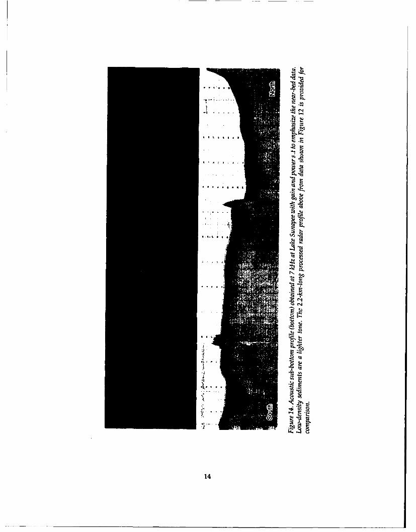
bottom detail .......................................................................................................... 1314. Acoustic sub-bottom profile obtained at 7 kHz at Lake Sunapee with

gain and power set to emphasize the near-bed data ......................................... 14

iii

Sub-bottom Surveying in Lakes with

Ground-Penetrating Radar

PAUL V. SELLMANN, ALLAN J. DELANEY AND STEVEN A. ARCONE

INTRODUCTION consideration given to frequency, power, deploy-ment and analysis of radiation patterns for maxi-

Information on the properties and distribution mum sub-bottom penetration.of sediments and rock beneath lakes, rivers and Radar used in conjunction with the acousticshallow backwaters is needed for geologic and method should allow one to obtain more completeengineering investigations. Harbor and channel sub-bottom data, since the two approaches haveprojects, sedimentation studies and general different temporal and spatial sensitivities and re-characterization of sub-bottom materials have re- spond to different physical properties. At a centerlied on acoustic methods because of their ability to frequency of 50 MHz the (typical) radar pulse usedpenetrate the bottom. However, acoustic equip- in these studies has a duration of about 50 ns, whichment can have difficulty in resolving gradational in water is about 1.7 m long, about three times thecontacts andinpenetratinggassy sediments, which length of the 7-kHz acoustic pulse that we used.can cause high attenuation (e.g., Fig. 1). Previous The 100-MHz radar pulse that we used was aboutfreshwater investigations using radar (Annan and 1.5 times the length of the acoustic pulse. Therefore,Davis 1977, Lowe 1985, Haeni et al. 1987, Gorin and the radar had theoretically less vertical resolutionHaeni 1989, Beres and Haeni 1991, Kovacs 1991) thanastandardacousticbottomsounder, butresolv-have revealed sub-bottom information. This report ing changes in the subsurface also depends ondiscusses radar equipment that we assembled with contrasts in material properties, which cause re-

Distance (m)210 220 230 240 250

I i I i I I I i

10-

20-

* at velocity of water

Figure 1. Acoustic section with a transition from sediments containing gas and no sub-bottom data toa gas-free zone in the center with low signal attenuation andgood sub-bottom returns (unpublished datacourtesy of W.J. Scott 1991).

flections. Contrasts for radiowave energy are re- stopped radiating. Electronics for the transmitterlated to variations in dielectric constant and electri- and receiver are usually incorporated into the an-cal resistivity. These contrasts can differ and in tenna housing. The VHF (30-300 MHz) receivedsome cases may exceed those at acoustic anoma- signals are converted by sampling into an audiolies, which depend on the product of density and frequency facsimile for filtering, amplification andcompressional wave velocity. This has been dem- recording. Data can be simultaneously displayedonstrated by successful use of resistivity methods or quickly played back in strip chart form. Digitalin investigations of coastal sub-sea permafrost recording is available, along with packaged signalwhere acoustic anomalies are difficult to detect processing software that permits several filtering(Sellmann et al. 1989, Scott and Maxwell 1989). functions and data display formats.

The primary objective of this research was todetermine the performance characteristics of our Antennas50-MHz system as a tool for obtaining sub-bottom The 50-MHz surveys were made with a pair ofdata. The results were compared with radar data compact, easily deployed antennas constructed atacquired with a commercially available 100-MHz CRREL and adapted for sub-bottom surveying.antenna unit and some preliminary acoustic data The antennas are linear dipoles, 2.05 m long, con-obtained at 7 kHz. The observations discussed in sisting of resistors placed at close intervals forthis report were made at three lake sites in New incremental loading. The resistor values used areHampshire. Both processed and unprocessed data based on theoretical developments of Wu and Kingare included. In some cases high quality sub-bot- (1964) and a design given by Watts and Wrighttom information was obtained without data pro- (1981). However, other experimentation* and ourcessing. However, signal processing substantially own experience has shown that the precise incre-improved the records when signal-to-noise ratios mental loading called for by the design is not aswere low. critical as the total resistive load. The antennas are

unshielded and produced the wavelet shown inFigure 2 with a 3-dB bandwidth of about 25% of the

RADAR EQUIPMENT 50-MHz center frequency, as determined by exactFourier transformation of a simulated waveform.

General operation The physical length of the pulse in water is aboutThe commercially available short-pulse radar 1.7 m. The transmit and receive antennas, along

equipment used for these observations was manu- with their electronics, were placed in separate wa-factured by Geophysical Survey Systems (GSSI, ter-tight plastic tubes 17 cm in diameter and 2.25 mNorth Salem, New Hampshire) and consisted of a long. The antennas were spaced 3.7 m apart bycontrol unit, magnetic tape recorder, power supply spreaders that positioned an antenna on each sideand a 100-MHz antenna unit containing both trans- of the boat and also allowed adjustments for an-mit and receive antennas. A 50-MHz antenna that tenna depth (Fig. 3). During operation, boat speedcould be used with the GSSI control unit was was about 4 kn (2 m/s) with the antennas 10 to 30constructed for this project and is discussed below. cm below the surface to maintain consistent cou-The control unit (SIR Model 4800) generates timing pling. Transmitter output was measured at 980 Wsignals to key the transmitter on and off and syn- against a 200-a load, but the actual antenna imped-chronizes this keying with the receiver. Transmit ance match to the water at any frequency was notpulses are triggered at a repetition frequency of determined.approximately 50 kHz. The unit also controls the The 100-MHz antenna unit (Model 3107, GSSI,scan rate (how fast individual echo scans are com- Inc.) radiates a wavelet (Fig. 2) with a frequencypiled-usually 25 scans/s), the time range over spectrum centered at 200 MHz in air and about 100which one wants to view the echoes (tens to thou- MHz when loaded by the proximity of the water.sands of nanoseconds), and the gain to be applied The physical length of the pulse in water is aboutto the echoes. The transmit antenna is excited by a 0.8 m. The 3-dB bandwidth is about 25%. Bothsemiconductor device and is designed to radiate a transmit and receive antennas (including electron-broadband pulse of 1.5 to 3 cycles duration. Conse-quently, the antenna produces a low gain radiationpattern. A separate, identical receive antenna isemployed because echoes can return from near- * Personal communication with J.L. Davis, Canpolar Inc.,surface targets before the transmit antenna has 1990.

2

' I I I I I I I I

50 MHz

S I I I i I I I I I

0 100 200 300 400 500Time (ns)

I I I I I I I I It 100 MHz

Figure 2. Pulse waveforms selectively am-plified within scans from records discussedlater. The 2.5 major cycles from the unshielded50-MHz antenna last about 54 ns and the 3 I I I 1 I I I Icycles from the shielded 100-MHz antenna 0 50 100 150 200 250last about 28 ns. Time (ns)

Figure 3. Fiberglass survey boat fitted with 50-MHz antennas (in tubes along gunnels)attached to vertical brackets for adjusting their position below the water surface. The 100-MHz antenna unit was placed inside the boat on the bottom and near the front for best couplingand separation from other equipment.

3

3000 3300360 300 600 300 ° 330* 3600 30 ° 60.

270 900 270* 90*

240* 120* 240° d* 120*

BW.= 900 BW.= 900

2100 1801 150* 210* 1800 1500

II to Antenna .I to Antenna(E Plane) (H Plane)

" "I0 - - - - 0

-4- -4-'

576° 56.3-

Depth 20mrE Depth=20m

Depth =20 mM p=S00L2-m " "p=5f-m

C

cc I r -

-10- 46.4- - 10-4

-20 -- 20 /

Depth =20 m Depth =20 mn" p=100 U-m- - p =1000-M"

-301 1 -301

20 10 0 10 20 20 10 0 10 20Distance (m) Distance (m)

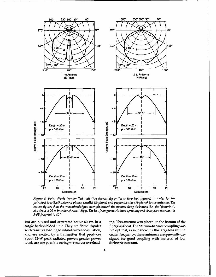
Figure 4. Point dipole transmitted radiation directivity patterns (top two figures) in water for theprincipal (vertical) antenna planes parallel (E-plane) and perpendicular (H-plane) to the antenna. Thebottom figures show the transmitted signal strength beneath the antenna along the bottom (i.e., the "footprint")at a depth of 20 n in water of resistivity p. The loss from geometric beamn spreading and absorption narrows the3-dB footprint to 40 .

ics) are housed and separated about 60 cm in a ing. This antenna was placed on the bottom of thesingle backshielded unit. They are flared dipoles fiberglassboat. Theantenna-to-watercoupling waswith resistive loading to inhibit current oscillation, not optimal, as evidenced by the large loss shift inand are excited by a transmitter that produces center frequency; these antennas are generally de-about 12-W peak radiated power; greater power signed for good coupling with material of lowlevels are not possible owing to receiver overload- dielectric constant.

4

0 Distance Figure4 areslightly modified when the finitelength_ . of the antennas is taken into account. For a linear

10- antenna, the H-plane pattern remains relativelyunchanged, but the E-plane pattern becomes morenarrow because of the interference effects of differ-

20 - ent parts of the radiating antenna. Appendix AE -gives the transmit/receive radar patterns of a vec-iF 30 - < tor addition of two 2-m linear arrays of point di-

poles, all balanced in strength according to the load

40 resistivity values, with the arrays separated 3.7 mas was done in the surveys. The patterns show thatour 50-MHz antennas produce an effective trans-

50 mit/receive 3-dB footprint at 20 m depth of only

Figure 5. Wiggle trace and equivalent line inten- 200 in the E-plane, comparable to the beamwidth,sity formats for graphic display. and about 470 in the H-plane. This focusing effect is

caused by the greater propagation distance to thesides of the antenna and the additional beam direc-

Subsurface radiation patterns for both antennas tivity factor upon reception. These transmit/re-are based on the theoretical and experimental re- ceive beamwidth values have been realized experi-sults for point dipoles by Annan et al. (1975) and mentally by Rossiter et al. (1991) using a smallEngheta et al. (1982). This theory shows the 3-dB spherical target in a tank.beamwidth of the radiation intensity from a singlepoint dipole to be confined within an angular width Data processing, displayof 90' in both principal radiation planes: the E- and interpretationplane and the H-plane (Fig. 4). The E-plane is The data were printed directly in the field dur-vertical and parallel to the antenna and the H-plane ing the observations using an EPC graphic recorderis also vertical but perpendicular to the antenna. to evaluate results and monitor equipment perfor-There is also a sharp null in the E-plane pattern in mance. This machine displays data in a gray scalethe direction w = 2 sin- 1 (/n), measured from the line intensity format (Fig. 5) that represents thevertical direction. The quantity n is the real part of pulse oscillations as a series of bands. The rawthe refractive index of water, which, at 23°C, equals analog data display from the EPC recorder, also9 so that w = 13'. The theory also shows the radia- used when digital filtering (to remove backgroundtion levels in air relative to those in water to be noise), removed some desired data. In addition allsuppressed by a fac[or equal to n. This reduction in data were recorded digitally on a GSSI DT6000 taperadiation to the air results in increased radiation to recorder for later processing and display. The re-the water (the antenna directivity in the vertical corder can store up to 65 megabytes of data in scansdirection is about 7 dB), resulting in a slightly of 512 or 1024 8-bit words on each tape. The digi-directive beam pattern in both principal planes, a tized data can be read onto a personal computer bydipole in air is directive only in the E-plane. For this a software program (Boucher and Galinovsky 1989)reason it was not necessary to shield the 50-M-lz that also processes the data. The program is ca-antennas from back radiation because of the low pable of a variety of filter functions, both horizontalradiation level in air. (i.e., over distance, or equivalently, many scans)

Figure 4 also shows the projected transmit foot- and vertical (i.e., over time, or equivalently, alongprint of a point dipole upon a flat lake bottom at a one scan). Data can be compressed by stacking ofdepth of 20 m, with water having resistivities simi- consecutive scans and displayed in either the wigglelar to those found at our study sites. The 3-dB width trace (amplitude versus time of each scan) or lineon the horizontal floor is first narrowed to about scan format. All raw data were stacked 6- to 8-fold690 in both planes because of the loss attributable to before digital filtering was applied. Individual scansthe greater distance traveled to the sides of the are easily retrievable with the software.antennas. In addition, attenuation caused by con- The graphic capability of the computer printerductive absorption further narrows this transmit- (HP Paintjet or Tektronix 4693DX) is, in a few cases,ted footprint to about 570 in 500-fl-m water, and to of poor quality, so that the weaker reflections seenabout 400 in 100-02-m water (Fig. 4), again because on the high resolution computer screen may beof the greater path length of radiation to the sides of barely visible after printing. Data interpretation isthe antennas. The point dipole patterns shown in generally based on the simple echo delay formula

5

d = ct/24E_ (1) gered time variable gain and a low-ring transducer.The time variable gain is triggered by the 200-kHz

where d = depth of a reflector (cm) bottom return to avoid false triggering by low-t = echo time delay (ns) frequency noise. The results are displayed in a linec = speed of electromagnetic waves in a intensity format on a survey fathometer (Model

vacuum (30 cm/ns) DE-719 RTr) that includes a compact dry paperE = n2 (relative dielectric constant). recorder capable of 30-cm resolution.

In this study sub-bottom acoustic informationThe factor of two in eq I accounts for the round trip was obtained with the 7-kHz transducer. The ra-propagation path of the pulse. Equation I applies diational directivity pattern and its equivalent bot-only to reflections from flat horizontal interfaces at tom footprint at 20 m depth are shown in Figure 6.least several wavelengths long, or to scattering Theeffective3-dB transmit footprintwidthona flatfrom point sources. It can be applied to several bottom is only about 320 and is slightly narrowerlayers successively if E is known for each layer, and than those of the point dipole seen in Figure 4. Theif the time delays to each interface are easily picked effective 3-dB transmit/receive footpnnt along aoff the record. flat bottom at 20 m depth is about 230 (Appendix

Signal attenuation with depth is caused by con- A). The pulse width was approximately 0.36 msductive and dielectric absorption, interface trans- (Fig. 6), which translates to about 54 cm or aboutmissions and spherical beam spreading. The beam two-thirds the length of the 100-MHz radar pulsespreading loss is compensated forby the automatic and one-third that of the 50.application of Time Range Gain (TRG), which ap-plies an amplitude gain that increases with time ofreturn or depth. Signal amplitude naturally de- RESULTScreases in inverse proportion to depth and the TRGapplied closely matched this loss for depths greater Three lakes located in central and west centralthan 8 m on the deeper surveys. New Hampshire were surveyed. The location of

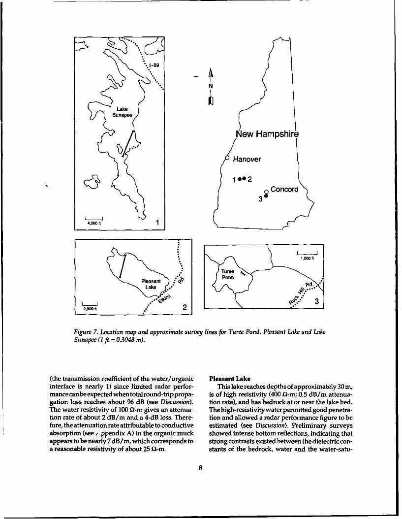
At any particular depth, the relative echo these lakes and the approximate location of thestrengths of lake bed returns are determined by the profile lines are shown in Figure 7. Turee Pond iscontrasts in dielectric constant between the water near the city of Concord. It ranges up to 3 m in(E = 81) and the sediments. For sediments, c is depth, is about 0.3 km 2 in area and was chosenassumed to depend on the relative volumetric ra- because of its shallow depth and soft organic bed.tios of solid and water; denser sediments would Pleasant Lake is near the town of New London andhave lower water content, a lower value of E and was selected for its depth and the occurrence ofproduce stronger reflections. Variations in sedi- bedrock at or near the lake bed. Lake Sunapee is ament density may also be distinguished along any large lake near the town of Newport and was alsoone scan where reflections become stronger with chosen for its depth and the low conductivity of thedepth. lake water. Site selection was aided by preliminary

radar surveys.

ACOUSTIC EQUIPMENT Turee PondThis pond contains low-density organic sedi-

A commercial sub-bottom acoustic survey sys- ment, has a shallow depth, conductive water andtern was used for one of the studies and was manu- abundant aquatic vegetation in the water column-factured by Ocean Data Systems (Fall River, Mas- features that should compromise the performancesachusetts), which supplied the specification given of both acoustic and radar techniques. Pond mar-below. The equipment was designed to obtain ac- gins are occupied by swampy, bog-like terrain withcurate bathymetric records and sub-bottom data in small trees and bushes established on parts of thewater depths of 5 to 120 m. High-frequency (200 bog surface. Shallow parts of the pond supportkHz) and dual low-frequency (Model TCA-3.5/7.0 very dense growths of aquatic vegetation and arekHz) transducers were mounted approximately 50 slowly being filled by peaty organic material. Ma-cm below the water surface off the side of the terial at and near the bed seems to consist primarilysurvey boat. The peak power output of the low- of dense to very fluid organic material with largefrequency transducer is 2000 W. The system fea- clumps of muck often found floating at the surface.tures include automatic initial and bottom-trig- A small area with a hard gravelly bottom was

6

0

05 -10

C

-15

-2020 10 0 10 20

Distance (m)

- UMENNEN

0.2 ms

Figure 6. Acoustic radiation directivity (left, top), and footprint pattern along a lake floor at adepth of 20 m (right, top). The bottom figure is the 7-kHz acoustic pulse shape with a durationof 0.36 ms for the major 2.5 cycles.

observed near the eastern shore and we assume the line the brightest returns are from the hardthat this material underlies the organic sediments gravelly layer below the bottom. Above these re-along our survey line. Accurate water depth was flections faint returns from the organic bed can bedifficult to determine with a sounding pole or line seen at both 50 and 100 MHz. All the data weresince little resistance was felt in the soft, fluid filtered to eliminate low-frequency noise, and thesediments. In some locations a boat-hook could be 100-MHz profile was further filtered using a two-pushed more than 50 cm into the bed with only dimensional Fourier transform to bring out thebarely perceptible resistance. The electrical resis- slanting bottom reflections.tivity of the pond water was measured at 100 Q-m. We estimate that at 50 MHz approximately 1 m

Figure 8 shows the results of a survey at two of water and 3.5 m of bed material were penetratedfrequencies for a line 200 m long. The depth scale is before signal strength from the denser sub-bottomlinear for the 100-MHz survey because the separa- layer was lost in the noise. At 4.5 m depth, the losstion of the transmit and receive antennas is small from beam spreading is about 31 dB and that fromcompared with the water depth. The depth scale reflection from the bottom of the saturated layer isfor the 50-MHz survey is not linear at these shallow estimated at 14 dB. This totals 45 dB and leavesdepths because of the 3.7-m antenna spacing. Along about 51 dB for losses in the water and organic layer

7

-. 1-89

LakeSunapee

New Hampshire

Hanover

1 oo2 Conc

4,000 It

-,11,000 ft

* Turee"Pon

Pleasant *bPn

Lake

2,000 ft 2 4~

Figure 7. Location map and approximate survey lines for Turee Pond, Pleasant Lake and LakeSunapee (1 ft = 0.3048 m).

(the transmission coefficient of the water/organic Pleasant Lakeinterface is nearly 1) since limited radar perfor- This lake reaches depths of approximately 30 m,mance can be expected when total round-trippropa- is of high resistivity (400 Q-m; 0.5 dB/m attenua-gation loss reaches about % dB (see Discussion). tion rate), and has bedrock at or near the lake bed.The water resistivity of 100 0-m gives an attenua- Thehigh-resistivity water permitted good penetra-tion rate of about 2 dB/m and a 4-dB loss. There- tion and allowed a radar perfoimance figure to before, the attenuation rate attributable to conductive estimated (see Discussion). Preliminary surveysabsorption (see ,. ppendix A) in the organic muck showed intense bottom reflections, indicating thatappears to be nearly 7 dB/m, which corresponds to strong contrasts existed between the dielectric con-a reasonable resistivity of about 25 0-m. stants of the bedrock, water and the water-satu-

8

0-

aF

4-

6-0-

1.5-

" 3.0-

0

4-6

6.0-

Figure 8. Processed data for the 50- and I00-MHz profiles from a 200-m line on the northeasternshore of Turee Pond. The arrows indicate the water/organic and organic/mineral interfaces. All profileshave been filtered to eliminate low-frequency noise. The 100-MHz profile on the left has been furtherprocessed using a two-dimensional Fourier transform filter to bring out the slanting bottom reflections. Thedepth scales are calibrated for water.

rated sediments. The bedrock was mapped as quartz tions of layering. In most cases it appears that themonzonite by Billings (1956), which, in our fre- bed surface, bedrock outcrops and the materialsquency range, has a dielectric constant of about 6 within the sedimentary bed produce strong reflec-(Campbell and Ulrichs 1969). tions. However, the change or absence of signal

Figure 9 is an unprocessed 50-MHz survey, 0.8 strength from within the bed indicates changes inkm long, near the west end of the lake made at a material properties, most likely related to density.time range of 1800 ns. It begins near the north side For example, at the southern end around location Aof the lake and extends to the south shore, passing and at the northern end around location B, it ap-a maximum depth of 21.5 m. The depth scale, pears that the irregular bedrock surface can bewhich is slightly nonlinear to about 20 m because of traced beneath the bed sediments. However, con-the 3.7-m separation of the antennas, is based on trasts in reflection strength (not apparent in thisthe value e = 81 for water. The constant horizontal black and white reproduction) at A suggest twobands across the record are the result of antenna distinct types of sediment (low density over highringing because of impedance mismatches between density), whereas at B the sediments appear thickerthe antenna and the water, and internal system and seem to contain more apparent layering. De-noise. These bands are easily removed by "back- tailed local information on sedimentation can alsoground removal" filtering (shown later), but were be seen in the center of the profile at location C,not removed from this figure because the (horizon- where sediments are deposited in a small basintal) filtering also tends to remove horizontal reflec- between rock knobs that extend above the bed.tions from flat portions of the lake bed. The B area in Figure 9 is shown in more detail in

This profile shows obvious features at and be- Figure 10. This section has been processed to re-low the bed, including bedrock outcrops, the bed- move the horizontal bands of background noiserock surface below the bed, contrasts in sediment and also variations in overall gain between scans.type and sedimentary patterns with strong indica- The section shows the irregular and fairly continu-

9

North

A

0 -S15-

20- . :

25-

South

10- A

CLE Bedrock15- C

25-

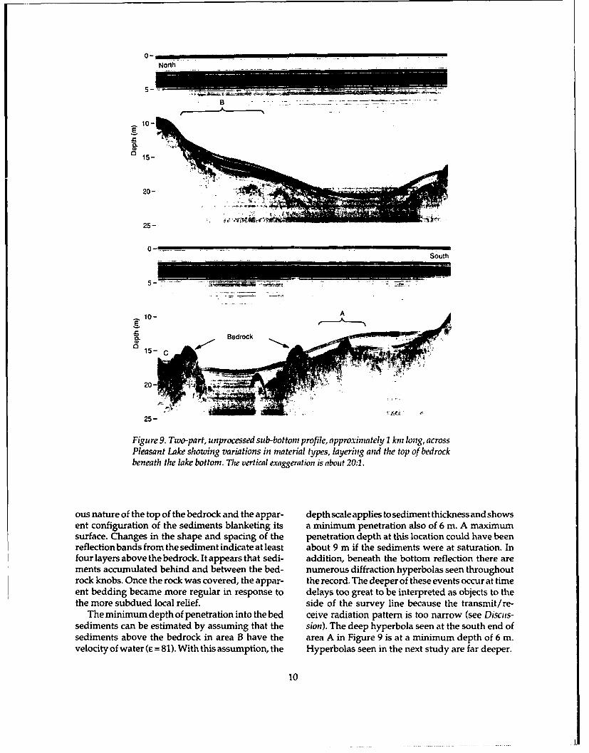
Figure 9. Two-part, unprocessed sub-bottom profile, approximately I km long, acrossPleasant Lake showing variations in material types, layering and the top of bedrockbeneath the lake bottom. The vertical exaggeration is about 20:1.

ous nature of the top of the bedrock and the appar- depth scale applies tosediment thickness and showsent configuration of the sediments blanketing its a minimum penetration also of 6 m. A maximumsurface. Changes in the shape and spacing of the penetration depth at this location could have beenreflection bands from the sediment indicate at least about 9 m if the sediments were at saturation. Infour layers above the bedrock. It appears that sedi- addition, beneath the bottom reflection there arements accumulated behind and between the bed- numerous diffraction hyperbolas seen throughoutrock knobs. Once the rock was covered, the appar- the record. The deeper of these events occur at timeent bedding became more regular in response to delays too great to be interpreted as objects to thethe more subdued local relief, side of the survey line because the transmit/re-

The minimum depth of penetration into the bed ceive radiation pattern is too narrow (see Discus-sediments can be estimated by assuming that the sion). The deep hyperbola seen at the south end ofsediments above the bedrock in area R have the area A in Figure 9 is at a minimum depth of 6 m.velocity of water (E = 81). With this assumption, the Hyperbolas seen in the next study are far deeper.

10

- 12

-16

.ECL

a)- 0

--20

- 24

230 m

Figure 10. Area B from Figure 9 processed to show more detailedinformation on the top of bedrock and the returns that suggestsedimentary layering. The irregular reflections at depth (apparent top ofbedrock) are less difficult to recognize after noise was suppressed.

Figures 11a and b compare 50- and 100-MHz Lake Sunapeeprofiles at the northern end of the Pleasant Lake Figures 12 and 13 show sub-bottom profilesline out to a water depth of 16 m where the 100- from the Sunapee line located in Figure 7. TheMHz returns are no longer visible. We made this maximum water depth along the survey line was

comparison to determine the improvement in reso- 20 m and several surface water samples gave alution of apparent sedimentary layering using the resistivity value of 500 Q-m, a value that gives onlyshorter 100-MHz pulse. Generally, layers whose 0.45 dB/m (one way) propagation attenuation at 50thickness corresponds to abouthalf thepulse width MHz. The bed is fairly flat, but interrupted bycan be resolved. This may be the case at location C, prominences at 0.4 km (reported by divers to bewhere there are twice as many bands for a given boulders) and 1.3 km (assumed to be bedrock).distance below the bed at 100 MHz as there are at 50 The strongest returns along the line are associ-MHz. (Each pulse band does not represent an indi- ated with the bedrock features and areas that ap-vidual layer since about 5 to 6 bands-positive and pear to consist of denser sediments; it appears thatnegativecycles-usually represent one pulse.)Thus, there are at least two different sediment typesthere is lessoverlapbetween reflections at 100 MHz along the line. Denser sediments with a strongerand better resolution. Detailed layering is sug- return appear at the bed along the southern part ofgested because the bands merge and spread, have the line (e.g., at 0.1-0.3 km and at 0.6-0.7 km).a logical configuration in relation to the rock, and Weaker returns, indicative of sediment of lowerare of fairly even intensity. These patterns suggest density, are evident in both processed and unproc-

significant contrasts in dielectric properties be- essed data and occur in the depressions at 0.0, 0.55tween layered sediments. and 0.75 km. Speaking quantitatively, given a nor-

11

Distance (km)0.06 0.08 0.10 0.12 0.14

1 I I I I I I I

0-

C

5-

E 10-

15-

20-

0.06 0.08 0.10 0.12 0.14II I I I I a I

0-

4-

E- 8-

CL

12-

16-

Figure 11. Comparison of a) 50-MHz profile, and b) 100-MHzprofile from the south end of the Pleasant Lake survey line shown inFigure 9.

malized peak-to-peak signal strength amplitude of the denser sediment (Fig. 13a) and stacked up1.0 for the denser sediments at 0.1-0.3 km, we see against the south side of the bedrock ridge near thethat the relative amplitudes at 0.0, 0.55 and 0.75 km center of the profile (Fig. 13b). It also can be seenare 0.33 (adjusted for extra conductive absorption completely covering the bed to the north of thisbecause of greater strength), 0.83 and 0.30 respec- ridge (Fig. 12 or 13b). We believe that the rapidtively. Amplitude changes attributable to varia- increase in signal strength on the north end indi-tions in depth alone were compensated for by the cates a hard sandy bottom. The low-density sedi-TRG, which closely matched theoretical changes ments with weak indications of bedding at thefrom spherical beam spreading. The denser ma- north end of Figure 12 appear to overlie more denseterial may be a till-like deposit containing some sediment that also has little apparent bedding.rocks and boulders, as suggested by the scattered As was seen in the Pleasant Lake data, there arehyperbolas at 0.1-0.2 and 0.6-0.7 km. The low- numerous diffraction hyperbolas that appear be-density material contains apparent bedding and lowthebottom.Theboulderpileat0.4kminFigureminorindication of small local reflectors. Processed 12 is the source of many of the diffractions in thisrecords show this material filling a depression in vicinity. However, there are some very deep dif-

12

0 0.2 0.4 0.6 0.8 1.0

0-

5-

0 15- - -' ;

20- - '. A

South25 - Distance (kin)1.2 1.4 1.8 2.0 2.2

-- -IIII I

0-

5-

15-

20 -

North25-

Figure 12. Unprocessed 50-MHz sub-bottom profile, 2.2 km long, from Lake Sunapee.

a. Low-density material filling a depres- b. Layered sediments deposited behind thesion in sediment of greater density lo- bedrock ridge at 1.3 km in the Lake Sunapeecated at 0.75 km in Figure 12. profile. The stronger returns from sediments

deposited between the bedrock irregularities adja-cent to the ridge suggest they have greater densitythan the overlying material.

Figure 13. Two processed sections from the Lake Sunapee profile illustrating sub-bottom detail.

13

to

~14

fractions between 0.30 and 0.35 km that we believe these loss calculations imply that with a high-may be sub-bottom, for reasons given in the Discus- reflectivity hard bedrock (E = 6) bottom and watersion. of similarly low conductivity, bottom returns well

Figure 14 allows comparison of the 50-MHz above noise could be obtained in water over 38 mradar data from Figure 12 with a 7-kHz acoustic deep. In 100-1-m water this depth decreases toprofile along the same line. The 7-kHz system was only about 12 m.set for the greatest sensitivity to returns from the In both the Pleasant Lake and Lake Sunapeenear-surface sediments, and the profile delineates data, there are sections with numerous hyperbolas,the upper and lower limits of the low-density de- many of which appear to emanate from beneath theposits much the same as shown in the radar data. bottom. The fact that some appear so deep (e.g.,However, the acoustic profile fails to show all the over twice the water depth) suggests that they maydetailed contrasts between types of bed material actually be on the bottom, but far to the side of theand any of the hyperbolic returns evident in the line. However, the amplitudes of these events areradar results. Since the acoustic pulse is about one- not consistent with radar range and attenuationthird the length of the radar pulse, the superior calculations (see Fig. Ala). For example, the dif-radar resolution could be ascribable to greater con- fraction event at 21 m depth at 0.32 km in Figure 12trastswithintheelectromagneticpropertiesascom- is only 10 dB weaker than the bottom reflection atpared to contrasts within the acoustic properties. 9 m depth. If this event was from the side of theFor example, indications of layering in the depres- antenna, the angle from vertical would be 650, atsions at 0.2 and 0.95 km can be seen in the radar which there is about 37 dB of loss in the radarrecord, but not in the acoustic data. The separation footprint pattern at 21 m distance. Since the TRGof these radar returns ranges from 50 to 80 ns, compensates for only the spherical spreading losswhich, for any dielectric constant corresponding to (about 15 dB from 9 to 21 m) to within 2 dB at thisa (30-70%) range in sediment water volume, allows depth, the amplitude observed is just too strong tothe layers to range from 1 to 3 m in thickness, a have the event come from off-center. Another pos-range that should be within the resolution capabili- sible explanation is that these events are within theties of the acoustic system. sub-bottom, but are less deep than they appear

because of unusually high dielectric constants inthe saturated sediments.

DISCUSSION The radar data and results of the preliminaryacoustic survey seen in Figure 14 provide an inter-

There are several factors that influence the per- esting comparison. The techniques confirm theformance of a radar, performance being defined as configuration of the low-density deposits near thethe ratioin decibels of theweakest detectablesignal bed. However, at these depths greater sub-bottomto the transmitted signal (see Appendix A). System detail is revealed in the radar profile. This increaselosses (e.g., mismatch at the water interface and in detail is most likely caused by greater electricalinternal cable reflections) are difficult to estimate. impedance contrasts at the sedimentary bound-However, losses from beam spreading, conductive aries; it cannot be attributed to a lack of clutter inabsorption and target reflectivity can be calculated the radar data as the acoustic system has a moreto estimate propagation loss and, therefore, the narrow effective beamwidth and a shorter pulsepenetration achieved in a freshwater survey. To length.make this calculation, we chose the greatest depthcrossed by any survey line (29 m, Pleasant Lake)where a bottom return was visible in the data. By CONCLUSIONS ANDuse of eq A3, at this depth the geometric beam RECOMMENDATIONSspreading gives 46 dB of loss, conductive and re-laxation absorption accounts for 31 dB (400--m Unprocessed radar data provided detailed in-water), and the bottom reflectivity gives 14 dB of formation on apparent sedimentary bedding andloss (assuming a water-saturated mineral sediment layering, sediment properties and distribution, andhaving an e = 36). This adds up to at least 91 dB of variations in depth to bedrock beneath the bed. Inpropagation loss for a round-trip return from the shallow lake water of low resistivity (100 fl-m),bottom. A hyperbolic reflection observed beneath low-density organic sediments, 1 to 4 m thick, werethe bottom return is evidence of a low-reflectivity profiled over denser bed material. In lake water ofbottom and additional power available. Therefore, higher resistivity (400-500 fl-m), bed penetration

15

to at least 6 m was obtained in water over 15 m Engheta, N., C. H. Pappas, and C. Elachi (1982)deep. Data processing provided significant im- Radiation patterns of interfacial dipole antennas.provements to the records, particularly where co- Radio Science, 17:1557-1566.herent noise levels were high. The radar and acous- Gorin, S.R. and F.P. Haeni (1989) Use of surface-tic techniques supported each other in confirma- geological methods to assess riverbed scour attion of gross sub-bottom features, while the radar bridge piers. U.S. Geological Survey Water Re-seemed to provide more detail for features near the sources Investigations Report 88-4212.bed. The 50-MHz system appears capable of detect- Haeni, F.P., D.K. McKeegan and D.R. Caproning signals that have suffered over 100 dB of propa- (1987) Ground-penetrating radar study of the thick-gation loss. ness and extent of sediments beneath Silver Lake,

The results presented are mainly qualitative, as Berlin and Meriden, Connecticut. U.S. Geologicalwe could not directly verify all sub-bottom condi- Survey Water Resources Investigations Report 85-tions at the three lakes investigated. Sub-bottom 4108.conditions (i.e., the depth of the organic layer) at Kovacs, A. (1991) Impulse radar bathymetric pro-Turee Pond are accessible and will be investigated filing in weed-infested fresh water. USA Cold Re-more thoroughly. A study of low-density organic- gions Research and Engineering Laboratory,mineral sediments is needed to estimate thickness. CRREL Report 91-10.This can be done either by calibration of the radar Lowe, D.J. (1985) Application of impulse radar torecord at selected points where the thickness can be continuous profiling of tephra-bearing lake sedi-directly measured, or by inserting waterproofed ments and peats: an initial evaluation. New Zea-antennas into the muck at a fixed separation and land Journal of Geology and Geophysics, 28: 667-674.measuring the time delay of the propagating pulse. Rossiter, J. I., E. M. Reimer, L. A. Lalumiere and

D. R, Inkster (1991) Radar cross section of fish. InProceedings of Workshop on Ground Penetrating Ra-

LITERATURE CITED dar, Ottawa, Canada, May 24-26, 1988 (J. A. Pilon,Ed.); also as Geological Survey of Canada paper 90-

Annan, A. P., W. M. Waller, D. W. StrangwayJ. R. 4,1990.Rossiter, J. D. Redman, and R. D. Watts (1975) The Scott, W. J. and F. K. Maxwell (1989) Marine resis-electromagnetic response of a low-loss, 2-layer, tivity survey for granular materials, Beaufort Sea.dielectric earth for horizontal electric dipole excita- Canadian Journal of Exploration Geophysics, 25(2).tion. Geophysics, 40(2): 285-298. Sellmann, P. V., A. J. Delaney and S. A. ArconeAnnan, A.P. and J.L. Davis (1977) Impulse radar (1989) Coastal subsea permafrost and bedrock ob-applied to ice thickness measurements and fresh- servations using dc resistivity. USA Cold Regionswater bathymetry. Geological Survey of Canada, Research and Engineering Laboratory, CRRELPaper 77-1B, p. 63-65. Report 89-13.Beres, M., Jr. and F.P. Haeni (1991) Application of Siggins, A. F. (1990) Experience with ground pen-ground-penetrating-radar methods in hydrologi- etrating radar in geotechnical applications. In Thirdcal studies. Ground Water, 29(3): 375-386. International Conference on Ground Penetrating Ra-Billings, M. P. (1956) The Geology of New Hampshire. dar, Lakewood, Colorado, May 14-18,1990, abstracts ofConcord, New Hampshire: Department of Re- the technical meeting (J. E. Lucius, G. R. Olhoeft and S.sources and Economic Development. K Duke, Eds.). USGS, Open-file Report 90-414, p. 6 2 .Boucher, R.and L.Galinovsky(1989) RADAN3.0, Watts, R. D. and D. L. Wright (1981) Systems forsignal processing software for the GSSI System. measuring thickness of temperate and polar iceNorth Salem, New Hampshire: Geophysical Sur- from the ground or from the air. Journal of Glaciol-vey Systems, Inc. ogy, 27(97): 459-469.Campbell, M. J. and J. Ulrichs (1969) Electrical Wu, T. T., and R. W. P. King (1964) The cylindricalproperties of rocks and their significance for lunar antenna with nonreflecting resistance loading. IEEEradar observations. Journal of Geophysical Research, Transactions ofAntennas Propagation, AP-12(3): 369-74(25): 5867-5881. 373.

16

APPENDIX A: RADAR RANGE EQUATION

The ratio of power received Pr from a finite reflector of cross section a, to power Pt radiatedby the transmitting antenna is

Pr/Pt = L G2%2 a e"40R/(64 X3 R4 ) W (L) (c) (G2 .2 /4n) (e "40R) (1 /l6n2R4) (Al)

where L = system losses (e.g., mismatches between cables and antennas or at the antenna/ground interface)

G = antenna gainX = transmitted wavelengthR = range to the target interface

= attenuation function of the propagation medium.

The third term in parentheses accounts for the antenna properties and evaluates to about-0.5 dB for the 50-MHz antenna in water. The fourth term accounts for conductive absorp-tion. The fifth term accounts for losses due to 1 /R 2 spherical spreading of the beam from thetransmitter to the target a, and then again from the target back to the receiver. The fact thatthe subsurface beam is directive in both radiation planes is accounted for in the antenna gain,which has a maximum of about 5 for an interface antenna radiating vertically downwardsinto water of refractive index n = 9. At 50 MHz the attenuation factor P is mainly determinedby conductivity (or its inverse resistivity) and is approximated for fresh water by the formula

= 1/(2pceon) (A2)

where p is water resistivity in Ql-m, and co is the permittivity of free space = 8.85 x 10-12 F/m. Amore exact calculation would consider the Debye relaxation of water.

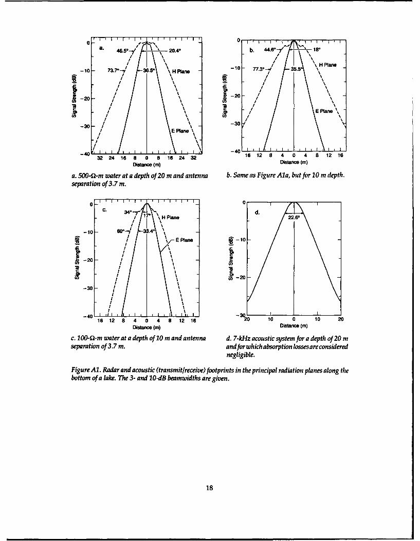
The last three factors in eq Al were used to compute the transmit/receive footprintsensitivity patterns for two 50-MHz, 2-m-long resistively loaded dipoles separated by 3.7 m(as used in the studies) with the transmit antenna excited by a unipolar current pulse. Thedirectivity patterns shown in Figure Al represent sensitivity to nondispersive, isotropicallyscattering objects along a flat bottom. For the depths considered, the radar patterns differinsignificantly for those for a single transmit/receive antenna. The energy values plotted arethe total energy in the pulse waveforms.

Figures Ala and b show that at 10-20 m depth in Lake Sunapee or Pleasant Lake, thereceived intensity decreases more rapidly with horizontal distances in the E-plane (parallelto the antenna and in the direction of the profiles) than it does in the H-plane, and the sidelobestructure seen earlier for point dipoles is greatly reduced. The narrower E-plane patternimplies that if any of the sub-bottom hyperbolas seen in the records are from off the vertical,they are more likely to have originated from the sides of the boat rather than fore and aft.Figure Alc is for a depth of 10 m in 100-f- water and Figure Ald is for the 7-kHz acoustictransducer. The highly absorptive (1.9 dB/m at 50 MHz) 100-f0-m water gives a morenarrow radar range footprint in both radiation planes, with the E-plane beamwidth morenarrow than that of the acoustic system.

The radar range equation for an infinite flat reflector takes the form given in eq A3, whichdoes not consider any system losses (L = 1).

Pr/Pt = (G X r)2 e"4pR/(64 n2 R2) = (G 2;.2 /4) (r2) (e-4 R) (1/16nR2). (A3)

The quantity r is the amplitude reflectivity of the water/bottom interface. The last threeterms in parentheses depend on the propagation and were used to compute the propagationlosses discussed in the text.

17

0 0a. 465 - 20.4° b. "6 8

/ /

-10 73-7'// 36.5 \ H Plane 10 77.3---4 H I

-I

- I

I \i

/

I

-20 I-20CaI

\. = I

.0 I \.0

S) / EPlane

-30 - // -304

//~ EPlane'

-40 142

32 24 16 8 0 8 16 24 32 1612840481216

Distance (m) Distance (m)

a. 500--m water at a depth of 20 m and antenna b. Same as Figure Ala, but for 10 m depth.separation of 3.7 m.

C. 34.0- 1. \ dH Plans 22.6

III

C

-10 - 60 *-" .4 \1

I a g)-20

-30.I

I

I a

I a

i aI

-40 -30'16 12 8 4 0 4 8 12 16 20 10 0 10 20

Distance (m) Distance (m)

c. 100-f2-m water at a depth of10 m and antenna d. 7-kHz acoustic system for a depth of 20 mseparation of 3.7 m. and for which absorption losses are considered

negligible.

Figure Al. Radar and acoustic (transmit/receive) footprints in the principal radiation planes along thebottom of a lake. The 3- and 10-dB beamwidths are given.

18

Form ApprovedREPORT DOCUMENTATION PAGE OMBNo. o7O4- 18PuI reopng oli n g othi ooieo of Inamnon is elmal iW awvqo 1 hour pr eone. l m b r g . .'ofg _V g da aM. ji6intirning the t needed, and coalvedg and revwing te 0lealot o W"one. sef commenla emgi a tie = %. d or any ade appe of e moion 4 1 a.

Inchdng auggeslin tr reduing tis butden. to Was eonot Headquenom Services. OlcrdOe " Opel d . 1215 eAN Dalei HigNwa. Suete 1204, Abilgof.VA 22202M402. and ID he Offe of Manageme and udget. Ppenowk Redimbon Pjed (0704-0185). Wlinglon. DC .

1. AGENCY USE ONLY (Leave blank) 2. REPORT DATE 3. REPORT TYPE AND DATES COVEREDMay 1992

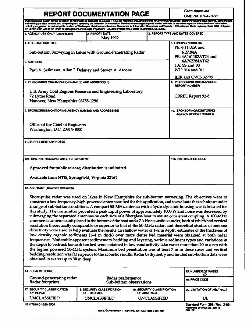
4. TITLE AND SUBTITLE 5. FUNDING NUMBERSPE: 6.11.02A and

Sub-bottom Surveying in Lakes with Ground-Penetrating Radar 6.27.84APR. 4A161102AT24 and

6. AUTHORS 4A762784AT42TA: SS and BS

Paul V. Sellmann, Allan J. Delaney and Steven A. Arcone WU: 014 and 011

ILIR and CWIS 327957. PERFORMING ORGANIZATION NAME(S) AND ADDRESS(ES) 8. PERFORMING ORGANIZATION

REPORT NUMBER

U.S. Army Cold Regions Research and Engineering Laboratory72 Lyme Road CRREL Report 92-8Hanover, New Hampshire 03755-1290

9. SPONSORINGMONITORING AGENCY NAME(S) AND ADDRESS(ES) 10. SPONSORINGWONITORINGAGENCY REPORT NUMBER

Office of the Chief of EngineersWashington, D.C. 20314-1000

11. SUPPLEMENTARY NOTES

12a. DISTRIBUTION/AVAILABILITY STATEMENT 12). DISTRIBUTION CODE

Approved for public release; distribution is unlimited.

Available from NTIS, Springfield, Virginia 22161

13. ABSTRACT (Maxmm 200 mr)

Short-pulse radar was used on lakes in New Hampshire for sub-bottom surveying. The objectives were toconstruct a low-frequency, high-powered antenna suited for this application, and to evaluate the technique undera range of sub-bottom conditions. A compact 50-MHz antenna with a hydrodynamic housing was fabricated forthis study. The transmitter provided a peak input power of approximately 1000 W and noise was decreased bysubmerging the separated antennas on each side of a fiberglass boat to assure consistent coupling. A 100-MI-zcommercial antenna unit placed in the bottom of theboat and a 7-kHz acoustic sounder, both of which had verticalresolution theoretically comparable or superior to that of the 50-MIHz radar, and theoretical studies of antennadirectivity were used to help evaluate the results. In shallow water of 1-2 m depth, estimates of the thickness oflow density organic sediments (1-4 m thick) over more dense bed material were obtained at both radarfrequencies. Noticeable apparent sedimentary bedding and layering, various sediment types and variations inthe depth to bedrock beneath the bed were obtained in low-conductivity lake water more than 20 m deep withthe higher powered 50-MIz system. Maximum bed penetration was at least 7 m in these cases and verticalbedding resolution was far superior to the acoustic results. Radar bathymetry and limited sub-bottom data wereobtained in water up to 30 m deep.

14. SUBJECT TERMS 15. NUMBERg PAGES

Ground-penetrating radar Radar performance 1s. PRICE CODERadar footprints Sub-bottom observations

17. SECURITY CLASSIFICATION 18. SECURITY CLASSIFICATION 19. SECURITY CLASSIFICATION 20. LIMITATION OF ABSTRACT

OF REPORT OF THIS PAGE OF ABSTRACT

UNCLASSIFIED UNCLASSIFIED UNCLASSIFIED UL

NSN 7540-01-280-5500 SWndwd Form 298 (Rev. 2-89)P eesaed by ANSI Si Z39-IS

*U.8. OVEWIMENT PRINTING OFFICE: 11 12 11= 2MI02