A.A. Jarai- Thermodynamic Limit of the Abelian Sandpile Model on Z^d

8/3/2019 A.A. Jarai- Thermodynamic Limit of the Abelian Sandpile Model on Z^d

http://slidepdf.com/reader/full/aa-jarai-thermodynamic-limit-of-the-abelian-sandpile-model-on-zd 1/24

Markov Processes Relat. Fields 11, 313–336 (2005)Markov MP RF &

ProcessesandRelated FieldscPolymat, Moscow 2005

Thermodynamic Limit of the Abelian

Sandpile Model on Zd

A.A. Jarai

Carleton University, School of Mathematics and Statistics, 1125 Colonel By Drive, Ottawa,ON K1S 5B6, Canada. E-mail: [email protected]

Abstract. We review basic properties of the Abelian sandpile model 1 and de-scribe recent progress made regarding its infinite volume limit on Zd. In par-ticular, we discuss the existence of the infinite volume limit of the stationarymeasure for d ≥ 2, existence of infinite volume addition operators for d ≥ 3,and construction of an infinite volume process for d ≥ 5. We give an overviewof the techniques relevant for these constructions.

Keywords: Abelian sandpile model, uniform spanning tree, thermodynamic limit,

waves, two-component spanning forest

AMS Subject Classification: 60K35, 82C22

1. Introduction

The Abelian sandpile, also known as the BTW model, was introduced byBak, Tang and Wiesenfeld [2, 3], as an example of a concept they termed self-

organized criticality (SOC). Although there is no mathematical definition of SOC, we can describe to what sort of models this term is usually applied. Thegeneral feature of SOC models is that they possess a stochastic dynamics thatdrives them towards a stationary state characterized by power law correlationsin space and time. The behaviour should be compared to that of lattice systemsof statistical physics at phase transition, such as critical percolation, where thesemodels exhibit power law spatial correlations.

In SOC models, criticality appears with a new flavour: correlations build upas a result of the dynamics. Various physical situations where the concept of

SOC may apply are described in the book [14].1This note is a somewhat extended version of the talk given at the workshop.



314 A.A. Jarai

The Abelian sandpile model (ASM) in particular has attracted a lot of at-

tention, due to its simple definition and rich structure. The dynamics is givenby a Markovian evolution of discrete height variables indexed by a finite set Λ.The mathematical study of the ASM was initiated by Dhar [5], who discoveredits Abelian property, and coined the name Abelian. He gave an algebraic andcombinatorial characterization of the configurations that occur in the station-ary state with positive probability. Since then several analytic results have beenobtained, for example, derivation of critical exponents on the Bethe lattice [8]and evidence of power law correlations [20]. Work of Majumdar and Dhar [21]revealed a correspondence between the sandpile model and the uniform span-ning tree. Using this connection, exact height probabilities were obtained intwo dimensions [24], and it was argued that the critical dimension of the modelis four [25]. See [6,7, 10] for reviews.

From the mathematical point of view, it is natural to consider the limit of

infinite Λ, and try to define the model in infinite volume. This question wasstudied in various settings by Maes et al. [16,17,19]. The content of these worksis reviewed in [18], which our paper is meant to complement.

The first part of our paper gives an introduction to the ASM, while thesecond part reports on recent progress regarding its infinite volume (thermody-namic) limit on Zd. We give a fairly detailed introduction to the basic propertiesof the model in Section 2. We focus on properties that are relevant for the infi-nite volume limit; no attempt was made to give a complete review. See [6,10,22]for additional introductory expositions. In Section 3, we give an overview of im-portant techniques, as well as a brief description of infinite volume results of Maes et al. In Section 4, we state the main results for the infinite volume limiton Zd. Section 5 presents the main ideas of the proofs. A key role in the proofsis played by the correspondence with spanning trees; reviewed in Section 3.3.

2. The model and its basic properties

2.1. The model

Let Λ ⊂ Zd be finite. Each site i ∈ Λ is assigned a positive integer height

variable zi. Values between 1 and 2d are called stable, values larger than 2d areunstable. We let ΩΛ = 1, . . . , 2dΛ denote the space of stable configurations.We are also given a probability distribution qΛ(i)i∈Λ on the set Λ. For muchof our discussion, the reader may assume that qΛ is the uniform distribution.

The configuration undergoes the following discrete time dynamics. If thecurrent state is zΛ ∈ ΩΛ, we choose a site i at random according to qΛ, andincrease the height at i by 1, that is

zi → zi + 1.



Thermodynamic limit of the Abelian sandpile model on Zd 315

If the new height is stable (≤ 2d), we have a new configuration in ΩΛ, and

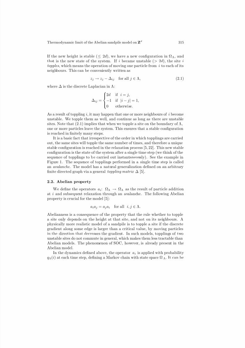
that is the new state of the system. If i became unstable (> 2d), the site itopples, which means the operation of moving one particle from i to each of itsneighbours. This can be conveniently written as

zj → zj − ∆ij for all j ∈ Λ, (2.1)

where ∆ is the discrete Laplacian in Λ:

∆ij =

2d if i = j,

−1 if |i − j| = 1,

0 otherwise.

As a result of toppling i, it may happen that one or more neighbours of i becomeunstable. We topple them as well, and continue as long as there are unstablesites. Note that (2.1) implies that when we topple a site on the boundary of Λ,one or more particles leave the system. This ensures that a stable configurationis reached in finitely many steps.

It is a basic fact that irrespective of the order in which topplings are carriedout, the same sites will topple the same number of times, and therefore a uniquestable configuration is reached in the relaxation process [5, 22]. This new stableconfiguration is the state of the system after a single time step (we think of thesequence of topplings to be carried out instantaneously). See the example inFigure 1. The sequence of topplings performed in a single time step is calledan avalanche. The model has a natural generalization defined on an arbitraryfinite directed graph via a general toppling matrix ∆ [5].

2.2. Abelian property

We define the operators ai: ΩΛ → ΩΛ as the result of particle additionat i and subsequent relaxation through an avalanche. The following Abelianproperty is crucial for the model [5]:

aiaj = ajai for all i, j ∈ Λ.

Abelianness is a consequence of the property that the rule whether to topplea site only depends on the height at that site, and not on its neighbours. Aphysically more realistic model of a sandpile is to topple a site if the discretegradient along some edge is larger than a critical value, by moving particlesin the direction that decreases the gradient. In such models, topplings of twounstable sites do not commute in general, which makes them less tractable than

Abelian models. The phenomenon of SOC, however, is already present in theAbelian model.

In the dynamics defined above, the operator ai is applied with probabilityqΛ(i) at each time step, defining a Markov chain with state space Ω Λ. It can be



316 A.A. Jarai

3 3 2 1

3 4 4 34 4 2 23 3 3 2

addition−→

3 3 2 1

3 4 4 34 4 3 23 3 3 2

addition−→

3 3 2 1

3 5 4 34 4 3 23 3 3 2

toppling ;

3 4 2 1

4 1 5 3

4 5 3 23 3 3 2

two topplings ;

3 4 3 14 3 1 4

5 1 5 23 4 3 2

two topplings ;

3 4 3 1

5 3 2 41 3 1 3

4 4 4 2

toppling ;

4 4 3 11 4 2 42 3 1 3

4 4 4 2

Figure 1. Illustration of the dynamics on a 4 × 4 lattice. Framed configurationsare stable. Framed sites represent particle addition or toppling. The secondparticle addition results in an avalanche of 6 topplings.

shown using the Abelian property that as long as qΛ(i) > 0 for all i ∈ Λ, there isa unique stationary distribution ν Λ. The stationary distribution is independentof qΛ, and uniform on the set of recurrent states of the Markov chain [5]. It iscommon to take qΛ to be uniform.

In studying the infinite volume dynamics, we run into the problem that thereis no uniform probability measure on Zd. A potential solution is to pass to a

continuous time model, where additions occur according to independent Poissonprocesses with rates ϕ(i)i∈Λ. One needs an assumption on the behaviour of ϕ(i) at infinity for the infinite volume dynamics to be well-defined. In partic-ular, for the standard model on Zd, ϕ has to go to zero sufficiently fast; seeTheorem 4.2 in Section 4. A uniform addition rate ϕ(i) ≡ constant is possiblefor so-called dissipative models; see Section 3.7.

2.3. Recurrent states

Let RΛ denote the set of recurrent states of the Markov chain. Then theoperators ai restricted to RΛ generate an Abelian group K Λ, and |K Λ| = |RΛ| =det(∆) [5]. In fact, K Λ is isomorphic to the factor group ZΛ/S Λ, where S Λ isthe additive subgroup of ZΛ generated by the rows of ∆. This property reflects

the rule (2.1). In fact, RΛ contains one representative from each co-set of S Λ,and therefore can be identified with K Λ in a natural way.




In addition to its algebraic aspect, RΛ has a combinatorial description.

Namely, one can characterize the transient states ΩΛ \ RΛ via forbidden sub-configurations (FSC). As an example, first consider a configuration in whichthere are two ones next to each other:

1 1 (2.2)

A simple argument shows that such a state cannot be recurrent. Indeed, aftersufficiently long time, at least one toppling has occurred at both sites. Afterthis time, either site can only be 1 between a toppling and the next particleaddition there. Therefore, the other site cannot be 1 at the same time. We callthe configuration in (2.2) an FSC.

The above example can be generalized. Let |A| denote the number of ele-ments of a set A. A configuration on a finite set F is called an FSC, if

zi ≤ | j ∈ F : j ∼ i| for all i ∈ F, (2.3)

where j ∼ i denotes that j and i are neighbours. For example,

12 2 2 31 1

is an FSC. A configuration in Λ is called allowed , if it contains no FSC. Itwas shown in [5] that recurrent states are allowed. The converse is also true,and can be proved in a number of ways. First, for sandpiles with a symmetrictoppling matrix, [21] gives a correspondence between allowed configurationsand spanning trees, whose number is det(∆), the same as |RΛ|. See Section 3.3

below about this correspondence. A more direct and more general proof waslater given by Speer [26], who generalized the notion of allowed configurationsto sandpiles with an arbitrary (not necessarily symmetric) toppling matrix, andshowed its equivalence to recurrence. Finally, [22] gives an alternative proof of the equivalence between allowed and recurrent configurations in the symmetriccase, without invoking the correspondence with spanning trees.

2.4. Expected number of topplings

We close the list of basic properties with a very useful observation of Dhar [5].Let

N Λ(i, j) = number of topplings at j caused by particle addition at i.

By the definition of the toppling procedure:

(aiz)j = zj + δij −k∈Λ

N Λ(i, k)∆kj . (2.4)



318 A.A. Jarai

Let Eµ denote expectation with respect to a probability measure µ. Averag-

ing (2.4) with respect to the invariant measure ν Λ, we getk∈Λ

EνΛ N Λ(i, k)∆kj = δij.

Therefore

EνΛ N Λ(i, j) = (∆−1)ijdef = GΛ(i, j) (Dhar’s formula). (2.5)

Here GΛ is (2d)−1 times the Green function of simple random walk in Λ, killedon exit from Λ.

2.5. Notation

We fix some more notation for the rest of the paper. We let Ω = 1, . . . , 2dZd

denote the set of stable configurations in infinite volume. We endow Ω with theproduct topology, which makes it into a compact metric space. Given a functionf (Λ) defined on all sufficiently large finite subsets of Zd, and taking values ina metric space with metric ρ, we say that limΛ→Zd f (Λ) = a, if for any ε > 0there exists Λ0 such that for all Λ ⊃ Λ0 we have ρ(f (Λ), a) < ε.

For K ⊂ Zd, we let F K denote the σ-field on Ω generated by the heightvariables in K . A local event (resp. local function ) is an event (resp. function)that belongs to F K for some finite K .

For i ∈ Λ, we let degΛ(i) = | j ∈ Λ : j ∼ i|.

2.6. Basic questions

A basic problem is to describe properties of avalanches under stationarity.

One can consider the following avalanche characteristics:

1) number of topplings in the avalanche (size);

2) number of sites toppled during the avalanche (range);

3) distance of the furthest toppled site from the start of the avalanche (ra-dius);

4) the maximum number of times a site topples (duration).

It is generally believed that the distributions of the above quantities obey powerlaws when d ≥ 2, in the thermodynamic limit Λ → Zd. More precisely, thismeans the following. Let S Λ denote one of the above four characteristics for anavalanche in the stationary ASM. That is, sample a configuration from ν Λ, drop

a particle at a fixed site, let’s say the origin, and let S Λ denote the value of thechosen quantity for this avalanche. It is expected that

limΛ→Zd

ProbS Λ = s = p(s),




where p(s) ∼ cs−τ , as s → ∞, for some constant c > 0 and critical exponent

τ > 0 depending on d and the chosen quantity.In trying to build a mathematical framework in which the above power laws

can be studied, one is led to the questions below; a program started in [16,17,19].

1) Does ν Λ have a (weak) limit ν as Λ → Zd?

2) Can one define the operators ai on ν -typical configurations?

3) Are avalanches ν -a.s. finite?

4) Does ai leave ν invariant?

5) Is there a natural infinite volume Markov process with invariant mea-sure ν ? Does it have good ergodic properties?

In the next section we give an overview of some results and techniques developedfor the ASM that are relevant for studying these questions.

3. An overview of results and techniques

3.1. The burning algorithm

There is a simple algorithm that checks whether a given configuration isallowed (and hence recurrent) [5]. We start the algorithm by declaring all sitesin Λ to be unburnt, and then successively burn sites whose height is largerthan the number of their unburnt neighbours. More formally, let A0 = ∅, theset of sites burning at time 0. If As has been defined for 0 ≤ s ≤ t, we letF t = Λ \ (∪t

s=0As), the set of unburnt sites after time t. We set

At+1 = i ∈ F t : zi > degF t(i).

At is the set of sites burning at time t; see Figure 2.It is not hard to show that the burning process recursively removes sites

that cannot be part of an FSC. If the process stops without burning all sites,the remaining configuration is an FSC. If all sites are burnt, then the initialconfiguration was allowed.

Note that the burning always starts at the boundary of Λ. In fact, we canthink of the fire starting at an artificially added site δ, usually called the sink .We connect δ to each i ∈ ∂ Λ by 2d − degΛ(i) edges. We denote this new graph

by Λ. We declare δ to be burning at time 0, set A0 = δ, and then proceedwith the same burning rule as before.

There is an equivalent way of thinking about the burning process. The

addition operators satisfy the relationsj∈Λ

a∆ij

j = id, i ∈ Λ,



320 A.A. Jarai

4 3 2 24 2 1 31 4 2 3

3 3 2 3

−→• 3 2 2• 2 1 3

1 4 2 3

• 3 2 •

−→• • 2 2• 2 1 3

1 4 2 •

• • 2 •

−→

• • 2 2

• 2 1 •

1 • 2 •• • • •

−→

• • 2 •• • 1 •• • • •• • • •

−→

• • • •

• • 1 •• • • •• • • •

Figure 2. Illustration of the burning algorithm on a 4 × 4 lattice. At each step,

framed sites are burnt.

where id is the identity element of K Λ. Multiplying these relations over i ∈ Λ,factors containing any i ∈ Λ \ ∂ Λ cancel. We get the relation

i∈∂ Λ

avii = id,

where vi =

j∈Λ ∆ij = 2d − degΛ(i). The latter expression is the number of neighbours of i in Λc. This means that adding vi particles to each boundarysite in a recurrent configuration triggers an avalanche that recreates the originalconfiguration. Alternatively, we can think of the avalanche being triggered bysending one particle along each edge emanating from δ. It is not hard to see

that in this avalanche, each site topples exactly once. Following the sequence of topplings is equivalent to the burning process.

3.2. Exact probabilities via determinants

We already mentioned that the number of recurrent states is |RΛ|=det(∆Λ).Using this determinantal formula in a subtle way, Majumdar and Dhar [20] gavea method for calculating the probabilities of certain configurations in the ther-modynamic limit Λ → Zd. To illustrate the method, consider the probabilityν Λ(z0 = 1) of having height 1 at a given site. Let x1, . . . , x2d denote the 2dneighbours of the origin. We modify Λ by removing the 2d − 1 edges connect-ing 0 to x2, . . . , x2d. We denote this modified graph by Λ. In Λ, 0 is connectedby the single edge 0x1 to the rest of the lattice. We modify the toppling matrix

accordingly, by setting∆

00 = ∆00 − (2d − 1) = 1;

∆xjxj = ∆xjxj − 1 = 2d − 1, (2 ≤ j ≤ 2d);




and

∆0xj = ∆

xj0 = 0, (2 ≤ j ≤ 2d).

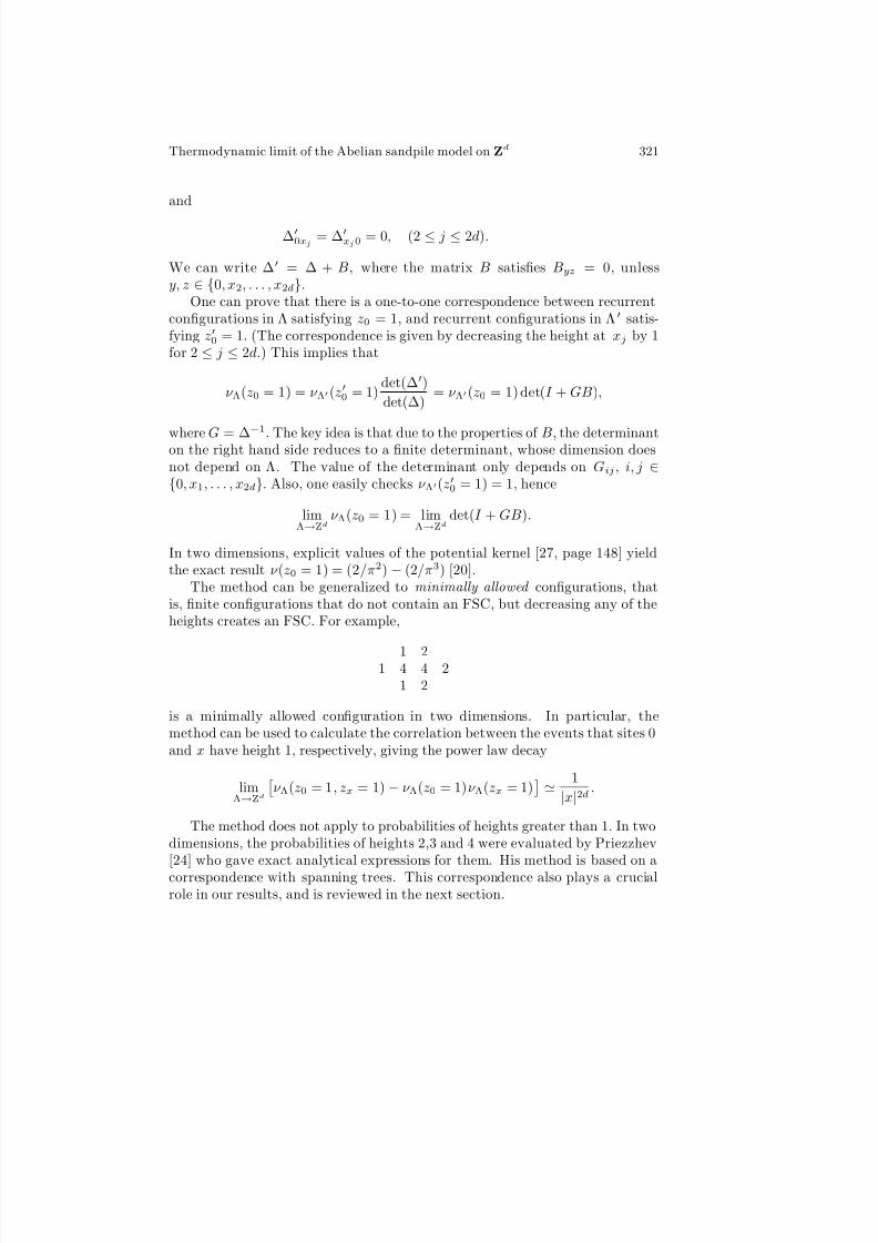
We can write ∆ = ∆ + B, where the matrix B satisfies Byz = 0, unlessy, z ∈ 0, x2, . . . , x2d.

One can prove that there is a one-to-one correspondence between recurrentconfigurations in Λ satisfying z0 = 1, and recurrent configurations in Λ satis-fying z0 = 1. (The correspondence is given by decreasing the height at xj by 1for 2 ≤ j ≤ 2d.) This implies that

ν Λ(z0 = 1) = ν Λ(z0 = 1)det(∆)

det(∆)= ν Λ(z0 = 1) det(I + GB),

where G = ∆−1

. The key idea is that due to the properties of B, the determinanton the right hand side reduces to a finite determinant, whose dimension doesnot depend on Λ. The value of the determinant only depends on Gij , i, j ∈0, x1, . . . , x2d. Also, one easily checks ν Λ(z0 = 1) = 1, hence

limΛ→Zd

ν Λ(z0 = 1) = limΛ→Zd

det(I + GB).

In two dimensions, explicit values of the potential kernel [27, page 148] yieldthe exact result ν (z0 = 1) = (2/π2) − (2/π3) [20].

The method can be generalized to minimally allowed configurations, thatis, finite configurations that do not contain an FSC, but decreasing any of theheights creates an FSC. For example,

1 21 4 4 2

1 2

is a minimally allowed configuration in two dimensions. In particular, themethod can be used to calculate the correlation between the events that sites 0and x have height 1, respectively, giving the power law decay

limΛ→Zd

ν Λ(z0 = 1, zx = 1) − ν Λ(z0 = 1)ν Λ(zx = 1)

1

|x|2d.

The method does not apply to probabilities of heights greater than 1. In twodimensions, the probabilities of heights 2,3 and 4 were evaluated by Priezzhev[24] who gave exact analytical expressions for them. His method is based on acorrespondence with spanning trees. This correspondence also plays a crucialrole in our results, and is reviewed in the next section.



322 A.A. Jarai

4 3 2 2

4 2 1 31 4 2 33 3 2 3

q q q q q q q q q q q q q q q q

q 3 2 2 q

2 1 31 4 2 3 q 3 2 q


q 2 2

2 1 31 4 2 q

q 2


2 22 1 q

1 q 2 q


2 q

q 1 q q


q

1


Figure 3. Spanning tree representation of the burning process on a 4 × 4 lattice.Framed sites are burnt at each step. Dots represent sites that were burnt in theprevious step. The outer box around each tree represents the vertex δ.

3.3. Spanning trees

In this section we describe a deep observation of Majumdar and Dhar [21]that relates the ASM to the uniform spanning tree (UST).

We follow the spread of fire in the burning process, and build a tree byconnecting each site to a neighbour that was burnt in the previous step. Here itwill be convenient to use the graph Λ introduced in Section 3.1. Recall that At

denotes the set of sites burning at time t. Observe that each i ∈ At (t ≥ 1) hasat least one neighbour in At−1, because sites become burnable after a certainnumber of their neighbours have been burnt. Below we define a rule that assignsto any i ∈ At a unique element of At−1, called the parent of i. Joining each site

to its parent then defines a spanning tree on Λ.The construction of the spanning tree is illustrated in Figure 3. In the first

step, four boundary sites were burnt (that is |A1| = 4), and these are connectedto δ (the only element of A

0) represented by a square drawn around Λ. Note

that for the three corner sites there are two possible edges to choose from, andwe have not yet specified how a choice is made. At each subsequent step, newlyburnt sites are connected to sites burnt in the previous step, marked by dots.




Now we specify how to choose the parent of i ∈ At. Let

ns(i) = |unburnt neighbours of i at time s|.

The number of neighbours of i ∈ At that are in At−1 is nt−1(i) − nt(i). Bythe burning rule, the possible height values at i consistent with i ∈ At arent < zi ≤ nt−1. Since the number of available neighbours is the same as thenumber of possible values of zi, we can assign a unique parent j ∈ At−1 to idepending on the value of zi. To be specific, let us order the 2d lattice directionsin a fixed way. Associating larger zi with larger lattice direction defines theparent uniquely.

In Figure 3, the directions were ordered as N > W > S > E. During the firststep, the site in the upper left corner having height 4 is burnt. The availableedges are in the directions N and W, and possible heights consistent with this

site being burnt at this stage are 3 and 4. Therefore the larger direction, Nwas chosen. At the two other corners having height 3, the smaller direction waschosen. The only other application of the rule occurs in step four, when a sitewith height 2 has two neighbours burnt in the previous step.

The above procedure results in a tree T Λ = φ(zΛ), which spans Λ if and onlyif the sets (At)t≥1 exhaust Λ. By the burning test of Section 3.1, this happensif and only if the configuration was recurrent. We regard δ as the root of thetree. At is precisely the set of sites at graph distance t from the root.

The procedure can be reversed to show that φ is a one-to-one mappingbetween recurrent configurations and spanning trees of Λ. We also describe φ−1

in detail. Given a spanning tree T Λ, let Bt denote the set of sites at graphdistance t from δ for t ≥ 0. Let mt( j) = #i : i ∼ j, i ∈ ∪t−1

r=0Br. For any j ∈ Bt, the number of neighbors of j in Bt−1 is mt−1( j) − mt( j). One of these

neighbors is the parent of j. We set the value of zj in such a way that for j ∈ Bt the inequalities mt( j) < zj ≤ mt−1( j) are satisfied, and we pick thatvalue which corresponds to the parent of j according to our fixed ordering of directions. It is clear that the resulting configuration zΛ is such that in theburning test At = Bt, nt( j) = mt( j) and φ(zΛ) = T Λ.

Since ν Λ gives equal weight to all recurrent states, the image of ν Λ under φis uniform on the spanning trees of Λ. This distribution is called the uniformspanning tree (UST) on Λ with wired boundary conditions [4,23]. “Wired” refersto the fact that the connection between two sites in T Λ may occur through theartificially added vertex δ (in contrast with “free” boundary conditions, whenconnections are required to occur within Λ). We denote the law of the wiredUST by µΛ. The next section describes the limit of µΛ as Λ → Zd.

3.4. The uniform spanning forest

It was shown by Pemantle [23] that as Λ → Zd, the uniform spanning treeconverges weakly to a limit called the uniform spanning forest (USF). The the-



324 A.A. Jarai

orem below summarizes this result together with an extension (statement 5)

proved in [4]. For more background on uniform spanning forests see [4].To state the theorem, it will be convenient to think of µΛ as a measure on

Ω = 0, 1Ed

, where Ed denotes the set of edges in Zd. We equip Ω withthe Borel σ-field with respect to the product topology. Elements of Ω can beviewed as subgraphs of (Zd, Ed), and any ω ∈ Ω defines a subgraph T Λ = T Λ(ω)

of Λ by identifying all vertices in Zd \ Λ to a single vertex and removing loops.Then µΛ is the unique measure under which T Λ is a.s. a tree and uniformlydistributed. We denote by T = T (ω) the set of edges present in ω ∈ Ω. We saythat an infinite tree has one end , if any two infinite paths have infinitely manyvertices in common.

Theorem 3.1. Let d ≥ 1. For any finite sets B ⊂ K of edges in Zd the limit

µ(T ∩ K = B)

def

= limΛ→Zd µΛ(T Λ ∩ K = B) (3.1)

exists, and uniquely defines a translation invariant measure µ on Ω. We have

µ = limΛ→Zd µΛ in the sense of weak convergence, and µ has the following

properties.

1) T has no cycles µ-a.s.

2) If d ≤ 4, T has a single component µ-a.s., that is, T is a tree µ-a.s.

3) If 2 ≤ d ≤ 4, T has one end µ-a.s.

4) If d > 4, T has infinitely many components µ-a.s., that is, T is a forest.

Each tree in T is infinite µ-a.s.

5) If d > 4, each component of T has a single end µ-a.s.

We call the random graph T governed by µ the USF, omitting referenceto the wired boundary condition. (In fact, on Zd the wired and free spanningforests coincide [4].)

Given the existence of limΛ→Zd µΛ, and the coding of sandpile configurationsby trees, it will not come as surprise that lim Λ→Zd ν Λ also exists, and the answerto Question 1 in Section 2.6 is affirmative; see Section 4 below. Theorem 3.1implies that in the case 2 ≤ d ≤ 4, we can think of T as a “rooted tree” with“root at infinity”. More precisely, statements 2 and 3 imply that for any j ∈ Zd

there is a unique infinite path j = v0, v1, . . . in T µ-a.s., and hence we can definethe parent of j to be v1. As we discuss in Section 5, this property of T allows usto extend the coding of sandpile configurations by trees to infinite volume. Thesituation is more subtle when d > 4, because the USF has multiple components.

As we describe in Section 5, a coding is still possible in this case, if we addto the USF a random ordering of its components. However, before discussingthese constructions in more detail, we place them into context by an overviewof related infinite volume results.




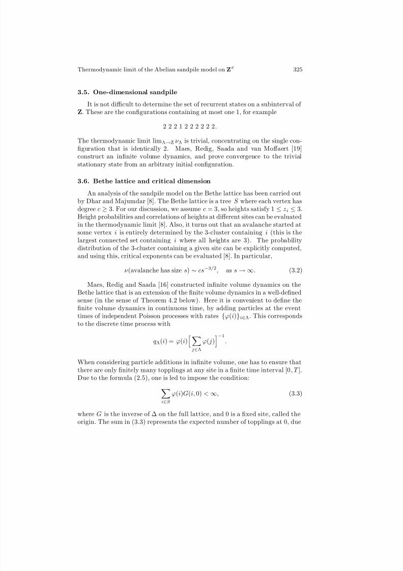
3.5. One-dimensional sandpile

It is not difficult to determine the set of recurrent states on a subinterval of Z. These are the configurations containing at most one 1, for example

2 2 2 1 2 2 2 2 2 2.

The thermodynamic limit limΛ→Z ν Λ is trivial, concentrating on the single con-figuration that is identically 2. Maes, Redig, Saada and van Moffaert [19]construct an infinite volume dynamics, and prove convergence to the trivialstationary state from an arbitrary initial configuration.

3.6. Bethe lattice and critical dimension

An analysis of the sandpile model on the Bethe lattice has been carried out

by Dhar and Majumdar [8]. The Bethe lattice is a tree S where each vertex hasdegree c ≥ 3. For our discussion, we assume c = 3, so heights satisfy 1 ≤ zi ≤ 3.Height probabilities and correlations of heights at different sites can be evaluatedin the thermodynamic limit [8]. Also, it turns out that an avalanche started atsome vertex i is entirely determined by the 3-cluster containing i (this is thelargest connected set containing i where all heights are 3). The probabilitydistribution of the 3-cluster containing a given site can be explicitly computed,and using this, critical exponents can be evaluated [8]. In particular,

ν (avalanche has size s) ∼ cs−3/2, as s → ∞. (3.2)

Maes, Redig and Saada [16] constructed infinite volume dynamics on theBethe lattice that is an extension of the finite volume dynamics in a well-defined

sense (in the sense of Theorem 4.2 below). Here it is convenient to define thefinite volume dynamics in continuous time, by adding particles at the eventtimes of independent Poisson processes with rates ϕ(i)i∈Λ. This correspondsto the discrete time process with

qΛ(i) = ϕ(i)j∈Λ

ϕ( j)−1

.

When considering particle additions in infinite volume, one has to ensure thatthere are only finitely many topplings at any site in a finite time interval [0, T ].Due to the formula (2.5), one is led to impose the condition:

i∈Sϕ(i)G(i, 0) < ∞, (3.3)

where G is the inverse of ∆ on the full lattice, and 0 is a fixed site, called theorigin. The sum in (3.3) represents the expected number of topplings at 0, due



326 A.A. Jarai

to particle additions in the time interval [0, 1]. Under condition (3.3), a Markov

process with invariant measure ν can be constructed [16]. Here ϕ(i) has to goto 0 sufficiently fast, as |i| → ∞, to make the sum convergent, and hence theaddition rate cannot be uniform.

It is expected that the behaviour on Zd is similar to the behaviour on theBethe lattice, for d > du, the upper critical dimension. In particular, critical ex-ponents on Zd for d > du would take on the same values as on the Bethe lattice.Priezzhev [25] argued that the upper critical dimension of the sandpile modelis du = 4. His arguments strongly support the conjecture that the asymptoticsin (3.2) holds on Zd when d > 4, and also in d = 4 with a logarithmic correction.

3.7. Dissipative models

Construction of the infinite volume limit has also been carried out for dis-

sipative models on Zd [17]. In our models so far, particles could only leave thesystem at boundary sites of Λ. If we modify ∆ by letting ∆ ii = γ > 2d, thenparticles will leave the system on toppling at any i. Stronger dissipation leads tofaster correlation decay, which makes the infinite volume limit more tractable.All questions in Section 2.6 can be answered in the affirmative; see [17] for moredetails.

4. The thermodynamic limit on Zd

In this section we consider the questions listed in Section 2.6 in the caseof Zd, d ≥ 2. We are able to answer all questions in the case d > 4, andwe address some of them when 2 ≤ d ≤ 4. The main ideas of the proofs aresummarized in Section 5.

Theorem 4.1. Let d ≥ 2. The limit ν = limΛ→Zd ν Λ exists in the sense of

weak convergence. ν is translation invariant, and there are no FSC’s ν -a.s.

In [1], Theorem 4.1 is proved when 2 ≤ d ≤ 4 and also when d > 4 withthe restriction that Λ is sufficiently regular, for example, the limit exists alongthe sequence of cubes Λn = [−n, n]d. The more general convergence result ford > 4 is proved in [13].

The proof is based on the correspondence with spanning trees given in Sec-tion 3.3 and the existence of the USF. When 2 ≤ d ≤ 4, Theorem 4.1 followsrather easily from Pemantle’s result, and a continuity argument. The coding of sandpile configurations by trees continues to hold in Zd in the following sense.There is a measurable (in fact µ-a.s. continuous) transformation Φ : Ω → Ω

that assigns a height configuration to any realization of the USF, such thatν = µ Φ−1; see [13]. When d > 4, the correspondence between the sandpilemodel and the USF breaks down on Zd. However, one can still encode sandpile




configurations, if one adds to the USF a random ordering of its components.

We explain these ideas in more detail in Section 5.1.

Remark 4.1.

(i) Let S Λ denote one of the avalanche characteristics introduced in Sec-tion 2.6. Then it follows that the limit

p(s) = limΛ→Zd

ν Λ(S Λ = s)

exists for s ≥ 0. We have

∞s=0

p(s) = 1 if and only if ν (infinite avalanche) = 0.

(ii) The limit p(s) is non-trivial for all d ≥ 2, by the method of Majumdarand Dhar described in Section 3.2. For example, in two dimensions theconfiguration

11 2 . . . 24 4 . . . 41 2 . . . 2

length s

2

produces an avalanche of size s, and is minimally allowed.

Given the existence of a unique thermodynamic limit ν , the next naturalstep is to define addition operators. First, define ai,Λ: Ω → Ω as the resultof applying the addition operator in volume Λ and leaving the configurationunchanged in Zd \ Λ. Recall that N Λ(i, j), i, j ∈ Λ denotes the number of

topplings at j caused by addition at i under the dynamics in Λ. With the abovedefinition of ai,Λ, we can also view N Λ(i, j) as a random variable on Ω. Withthese conventions, the following is proved in [13].

Proposition 4.1. For any i, j ∈ Zd, the limit limΛ→Zd N Λ(i, j) = N (i, j) ≤ ∞exists on Ω, and

Eν N (i, j) ≤ limΛ→Zd

GΛ(i, j) = G(i, j).

If d > 2, N (i, j) is finite ν -a.s., and limΛ→Zd ai,Λ = ai exists ν -a.s.

In the above proposition, the important ingredient is that when d > 2, theexpected number of topplings (and therefore the number of topplings) at all sitesis finite ν -a.s. This is sufficient to define ai, but does not imply that avalanchesare finite.

We can proceed further, if we know that avalanches are ν -a.s. finite2

. Wecan prove this at least when d > 4; see Proposition 4.3 below.

2Russell Lyons informed us (private communication) that it is possible to prove item 1 of Proposition 4.2 based only on transience, that is when d > 2.



328 A.A. Jarai

Proposition 4.2. Assume that avalanches are ν -a.s. finite. Then the following

statements hold.

1) ν is invariant under ai, i ∈ Zd.

2) Eν N (i, j) = G(i, j) (extension of Dhar’s formula ).

3) aiaj = ajai, ν -a.s. (Abelian property ).

4) a−1i exists ν -a.s.

5) For any i ∈ Zd and for ν -a.e. z ∈ Ω, there exist finite sets V i(z), W i(z),

such that aiz = ai,Λz for Λ ⊃ V i(z), and a−1i z = a−1

i,Λz for Λ ⊃ W i(z).

The proof of the above proposition is fairly independent of the model, andis based on techniques developed in [16, 17]. The key step then is to prove the

following proposition.

Proposition 4.3. If d > 4, there are no infinite avalanches ν -a.s.

Proposition 4.3 is proved in [13]. We describe the main ideas of its proof in Section 5.3. Given the results of Propositions 4.3 and 4.2, we can invokethe machinery developed in [16] to construct a Markov process with invariantmeasure ν . Using this machinery, one can prove the theorem below that appearsin [13].

Theorem 4.2. Assume d > 4. Let ϕ : Zd → (0, ∞) be an addition rate such

that i∈Z

d

ϕ(i)G(0, i) < ∞.

Then the following statements hold.

1) The closure of the operator on L2(ν ) defined on local functions by

Lϕf =i∈Zd

ϕ(i)(ai − I )f

is the generator of a stationary Markov process ηt : t ≥ 0.

2) Let N ϕt (i)i∈Zd be independent Poisson processes with rates ϕ(i), gov-

erned by the probability measure P. The limit

ηt = lim

Λ→Zd

i∈Λ

aN ϕt (i)i,Λ

η

exists P×ν -a.s. Moreover, ηt is a cadlag version of the process with gen-

erator Lϕ.




One would also like to investigate ergodic properties of both ν and the con-

structed Markov process. We recall the definition of tail triviality. The tail σ-field is defined to be

F ∞ =

Λ

F Zd\Λ,

where the intersection is over all finite subsets of Zd. A measure µ is tail trivial ,if µ(A) = 0 or 1 for every A ∈ F ∞. Tail triviality implies mixing under spatialtranslations. The following theorem is proved in [13]; see Section 5.4 below forthe main ideas of its proof.

Theorem 4.3. ν is tail trivial for any d ≥ 2.

Finally, as a consequence of Theorem 4.3 we can prove that the sandpileprocess in infinite volume is mixing in time; see [13].

Theorem 4.4. Let d > 4. The process ηt : t ≥ 0 of Theorem 4.2 is mixing.

5. Main ideas of the proofs

5.1. Existence of limΛ→Zd ν Λ

We start by outlining the ideas behind Theorem 4.1. Recall from Section 3.3the procedure that recovers the sandpile configuration from T Λ. The followingobservation plays an important role.

In order to reconstruct zj from T Λ, it is enough to know the distance of jfrom the root of T Λ relative to the distances of its neighbors from the root. Weexplain this in more detail. Recall that Bt is the set of sites at graph distance t

from the root. Let N denote the set of neighbours of j. Define the indices t andt(i), i ∈ N , by the conditions j ∈ Bt and i ∈ Bt(i), i ∈ N . Let i0 denote theparent of j, so that t(i0) = t − 1. By the construction of T Λ, zj is determinedby i0 and the following two sets:

A = i ∈ N : t(i) ≤ t − 1

B = i ∈ N : t(i) = t − 1 i0.(5.1)

A consists of those neighbours of j that burned before j, and B of those thatburned one step before j. In particular, i0 and the set of integers t(i) − ti∈N determines zj , even without knowing the value of t.

The above observation allows us to reconstruct zj knowing only a smallportion of T Λ. For example, let vΛ denote the earliest common ancestor of the

vertices in N , that is the first vertex common to all paths leading from N to δ.Let F Λ denote the subtree of T Λ consisting of the paths leading from j ∪ N to vΛ. In other words, (F Λ, vΛ) is the smallest rooted subtree of T Λ containing



330 A.A. Jarai

j ∪ N . The pair (F Λ, vΛ) already determines zj . This is because, letting dist

denote graph distance,

t(i) − t = distF Λ(i, vΛ) − distF Λ( j,vΛ), i ∈ N ,

and i0 is the parent of j in the rooted tree (F Λ, vΛ).It turns out that when 2 ≤ d ≤ 4, the distribution of vΛ is tight, that is for

any ε > 0 there exists a finite set K = K (ε) ⊂ Zd such that µΛ(vΛ ∈ K ) ≥ 1 − εfor all Λ ⊃ j ∪ N . Hence F Λ remains “localized” near j. More precisely,statements 2 and 3 of Theorem 3.1 imply that for any k ∈ Zd there exists aunique infinite path k = v0, v1, v2, . . . in T µ-a.s. Defining v1 to be the parentof k, we can regard T as a “rooted tree” with “root at infinity”. Therefore wecan define infinite volume analogues of vΛ and F Λ µ-a.s. Namely, the paths inT from j ∪ N to infinity will have a first common vertex v µ-a.s., and wedefine F as the union of the paths in T from j ∪ N to v. One can show that

(F Λ, vΛ) converges weakly to (F, v). This leads to the fact that the limitingdistribution of zj as Λ → Zd is determined by (F, v). Generalizing this idea,one can show that the coding of sandpile configurations by trees extends to theinfinite volume.

In the case d > 4, the USF has multiple components, and therefore v and F cannot be defined µ-a.s. In this case the probability that vΛ = δ is bounded awayfrom 0, and hence the distribution of vΛ is not tight. We modify the definitionsgiven for 2 ≤ d ≤ 4 by subdividing T Λ into “components”. With slight abuse of language, we say that x, y ∈ Λ are connected , if the path in T Λ from x to y doesnot pass through δ (that is, if they are connected in the usual graph-theoreticsense in the graph obtained by removing δ). Let A(1), . . . , A(r) be the (random)partition of j ∪ N into mutually disconnected subsets. In other words, theA(α) are the non-empty intersections of j ∪ N with connected componentsof T Λ; see Figure 4. We use a fixed deterministic rule to index elements of the

partition. Analogously to the case 2 ≤ d ≤ 4, we define (F (α)Λ , v

(α)Λ ), α = 1, . . . , r ,

as the smallest rooted subtree of T Λ containing A(α). Now zj is a function of

(F (α)Λ , v

(α)Λ )rα=1 and the distances

X (α)Λ = distT Λ(v

(α)Λ , δ), α = 1, . . . , r .

This because

t(i) − t = distF (

α)Λ

(i, v(α)Λ ) + X

(α)Λ − dist

F (β)

Λ( j,v

(β)Λ ) − X

(β)Λ (5.2)

if i ∈ A(α) and j ∈ A(β).

Fortunately, we only need rough information about X (α)Λ , α = 1, . . . , r. To

see this, observe that A and B in (5.1) are already determined by the linear

ordering of the integers t(i) − ti∈N (if we know i0), since

A = i ∈ N : t(i) − t ≤ t(i0) − t

B = i ∈ N : t(i) − t = t(i0) − t.




r r r r r

r r r r r r r r r r

r r

Λ

ji0

i1

i2

i3

v(2)Λ

v(1)Λ

F (1)Λ F

(2)Λ

Figure 4. Imitation of the case d > 4 in a two-dimensional picture. i0 isthe parent of j, and i1, i2, i3 are the other neighbours of j. There are twoconnected components intersecting j ∪ N = j,i0, . . . , i3. The intersections

are A(1) = j,i0, ii and A(2) = i2, i3. Thick lines represent the subtrees F (1)Λ

and F (2)Λ . Thin lines indicate the (disjoint) connections from these trees to the

boundary.

If i1, i2 ∈ A(β), then the order between t(i1) − t and t(i2) − t only depends

on (F (β)Λ , v

(β)Λ ). When i1 ∈ A(β) and i2 ∈ A(γ) for β = γ , then due to (5.2),

the order depends on (F (β)Λ , v

(β)Λ ), (F

(γ)Λ , v

(γ)Λ ) and the difference X

(β)Λ − X

(γ)Λ .

However, for large Λ, we expect that typically

min1≤β<γ≤r

X (β)Λ − X

(γ)Λ

max1≤α≤r

diam(F (α)Λ ), (5.3)

where diam denotes graph diameter. Therefore, when (5.3) holds, the order

between t(i1) − t and t(i2) − t will only depend on whether X (β)Λ > X

(γ)Λ or

X (β)Λ < X

(γ)Λ . Therefore, only the order between X

(α)Λ rα=1 is relevant in the

limit Λ → Zd. It turns out that the order is asymptotically uniform over all

permutations of 1, . . . , r, given r and (F (α)

Λ , v(α)Λ )rα=1. In proving that the

picture in (5.3) is indeed correct, we rely on Wilson’s algorithm, reviewed inSection 5.2 below; see [1] for details.

We can construct a coding of the sandpile model in terms of the USF based

on the results described above; stated explicitly in [13]. Let T (1)

, . . . , T (r)

denotethe components of the USF that have a non-empty intersection with j ∪ N .

Define the infinite volume analogues of (F (α)

Λ , v(α)Λ )rα=1 by letting (F (α), v(α))

be the smallest subtree of the USF containing ( j ∪ N ) ∩ T (α). We consider




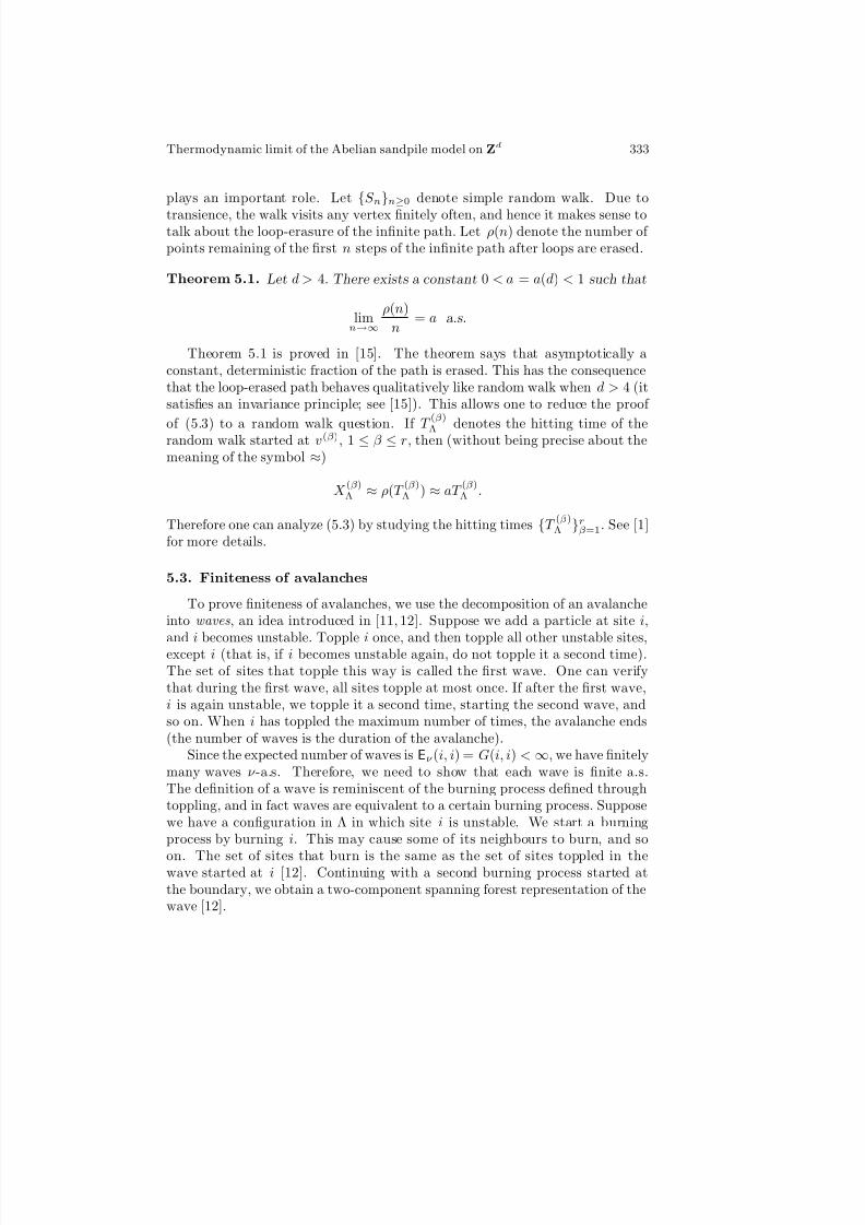
plays an important role. Let S nn≥0 denote simple random walk. Due to

transience, the walk visits any vertex finitely often, and hence it makes sense totalk about the loop-erasure of the infinite path. Let ρ(n) denote the number of points remaining of the first n steps of the infinite path after loops are erased.

Theorem 5.1. Let d > 4. There exists a constant 0 < a = a(d) < 1 such that

limn→∞

ρ(n)

n= a a.s.

Theorem 5.1 is proved in [15]. The theorem says that asymptotically aconstant, deterministic fraction of the path is erased. This has the consequencethat the loop-erased path behaves qualitatively like random walk when d > 4 (itsatisfies an invariance principle; see [15]). This allows one to reduce the proof

of (5.3) to a random walk question. If T

(β)

Λ denotes the hitting time of therandom walk started at v(β), 1 ≤ β ≤ r, then (without being precise about themeaning of the symbol ≈)

X (β)Λ ≈ ρ(T

(β)Λ ) ≈ aT

(β)Λ .

Therefore one can analyze (5.3) by studying the hitting times T (β)Λ rβ=1. See [1]

for more details.

5.3. Finiteness of avalanches

To prove finiteness of avalanches, we use the decomposition of an avalancheinto waves, an idea introduced in [11, 12]. Suppose we add a particle at site i,

and i becomes unstable. Topple i once, and then topple all other unstable sites,except i (that is, if i becomes unstable again, do not topple it a second time).The set of sites that topple this way is called the first wave. One can verifythat during the first wave, all sites topple at most once. If after the first wave,i is again unstable, we topple it a second time, starting the second wave, andso on. When i has toppled the maximum number of times, the avalanche ends(the number of waves is the duration of the avalanche).

Since the expected number of waves is Eν(i, i) = G(i, i) < ∞, we have finitelymany waves ν -a.s. Therefore, we need to show that each wave is finite a.s.The definition of a wave is reminiscent of the burning process defined throughtoppling, and in fact waves are equivalent to a certain burning process. Supposewe have a configuration in Λ in which site i is unstable. We start a burningprocess by burning i. This may cause some of its neighbours to burn, and so

on. The set of sites that burn is the same as the set of sites toppled in thewave started at i [12]. Continuing with a second burning process started atthe boundary, we obtain a two-component spanning forest representation of thewave [12].



334 A.A. Jarai

To show that waves remain finite in the limit Λ → Zd, we show that the

component of the two-component spanning forest containing i remains finite inthis limit, at least when d > 4. The proof of this again uses Wilson’s algorithm.

5.4. Tail triviality

The proof of Theorem 4.3 in the case 2 ≤ d ≤ 4 is a rather easy consequenceof the tail triviality of the USF [4], and the fact that each height variable onlydepends on an a.s. finite portion of the USF. The main technical difficulty inthe case d > 4 is the presence of the random ordering, which prevents us fromusing tail triviality of the USF directly. We show the following statement thatis equivalent to tail triviality. For any local event A and ε > 0 there is a finiteset K = K (A, ε) such that for any B ∈ F Zd\K :

|ν (A ∩ B) − ν (A)ν (B)| ≤ ε. (5.4)

Translated into the language of the USF, establishing (5.4) roughly amountsto showing the following. Given the configuration of the USF outside some largeset Λ, and given the order of the components, the conditional distribution of

(F (α)Λ , v

(α)Λ )rα=1 and the order of the components containing them, is close to its

unconditional distribution. See [13] for details.

Acknowledgments

I thank Siva Athreya and Frank Redig for fruitful collaborations leading tothe results discussed in this paper. I also thank Thierry Gobron and Ellen Saadafor organizing a very interesting conference and providing the incentive to write

these notes. I am grateful to Ellen Saada and the referee for helpful comments.The first version of this paper was written at CWI, Amsterdam.

References

[1] S.R. Athreya and A.A. Jarai (2004) Infinite volume limit for the stationarydistribution of Abelian sandpile models. Commun. Math. Phys. 249, 197–213.An Erratum is to appear, correcting some mistakes discovered in the paper.

[2] P. Bak, C. Tang and K. Wiesenfeld (1987) Self-organized criticality: Anexplanation of the 1/f noise. Phys. Rev. A 59, 381–384.

[3] P. Bak, C. Tang and K. Wiesenfeld (1988) Self-organized criticality. Phys.

Rev. A 38, 364–374.

[4] I. Benjamini, R. Lyons, Y. Peres and O. Schramm (2001) Uniform spanningforests. Ann. Prob. 29, 1–65.

[5] D. Dhar (1990) Self-organized critical state of sandpile automaton models. Phys.

Rev. Lett. 64, 1613–1616.




[6] D. Dhar (1999) The Abelian sandpile and related models. Physica A 263, 4–25.

[7] D. Dhar (1999) Studying self-organized criticality with exactly solved models.Preprint. http://arXiv.org/abs/cond-mat/9909009.

[8] D. Dhar and S.N. Majumdar (1990) Abelian sandpile model on the Bethelattice. J. Phys. A 23, 4333–4350.

[9] D. Dhar, P. Ruelle, S. Sen and D.N. Verma (1995) Algebraic aspects of Abelian sandpile models. J. Phys. A 28, 805–832.

[10] E.V. Ivashkevich and V.B. Priezzhev (1998) Introduction to the sandpilemodel. Physica A 254, 97–116.

[11] E.V. Ivashkevich, D.V. Ktitarev and V.B. Priezzhev (1994) Critical expo-nents for boundary avalanches in two-dimensional Abelian sandpile. J. Phys. A

27, L585–L590 (1994).

[12] E.V. Ivashkevich, D.V. Ktitarev and V.B. Priezzhev (1994) Waves of

topplings in an Abelian sandpile. Physica A 209, 347–360.[13] A.A. Jarai and F. Redig (2004) Infinite volume limits of high-dimensional

sandpile models. Preprint. To appear in Probab. Theory and Relat. Fields.

[14] H.J. Jensen (2000) Self-organized Criticality. Emergent Complex Behavior in

Physical and Biological Systems. Cambridge Lect. Notes Phys. 10. CambridgeUniversity Press.

[15] G.F. Lawler (1996) Intersections of Random Walks. Birkhauser.

[16] C. Maes, F. Redig and E. Saada (2002) The Abelian sandpile model on aninfinite tree. Ann. Prob. 30, 2081–2107.

[17] C. Maes, F. Redig and E. Saada (2004) The infinite volume limit of dissipativeabelian sandpiles. Commun. Math. Phys. 244, 395–417.

[18] C. Maes, F. Redig and E. Saada (2004) Abelian sandpiles in infinite volume.

Preprint. To appear in Sankhy¯ a, The Indian Journal of Statistics.[19] C. Maes, F. Redig, E. Saada and A. van Moffaert (2000) On the thermo-

dynamic limit for a one-dimensional sandpile process. Markov Processes Relat.

Fields 6, 1–22.

[20] S.N. Majumdar and D. Dhar (1991) Height correlations in the Abelian sandpilemodel. J. Phys. A 24, L357–L362.

[21] S.N. Majumdar and D. Dhar (1992) Equivalence between the Abelian sandpilemodel and the q → 0 limit of the Potts model. Physica A 185, 129–145.

[22] R. Meester, F. Redig and D. Znamenski (2002) The Abelian sandpile; amathematical introduction. Markov Processes Relat. Fields 7, 509–523.

[23] R. Pemantle (1991) Choosing a spanning tree for the integer lattice uniformly.Ann. Prob. 19, 1559–1574.

[24] V.B. Priezzhev (1994) Structure of two-dimensional sandpile. I. Height Proba-bilities. J. Stat. Phys. 74, 955–979.

[25] V.B. Priezzhev (2000) The upper critical dimension of the Abelian sandpilemodel. J. Stat. Phys. 98, 667–684.



336 A.A. Jarai

[26] E.R. Speer (1993) Asymmetric Abelian sandpile models. J. Stat. Phys. 71,

61–74.[27] F. Spitzer (1976) Principles of Random Walk . Graduate Texts in Mathemat-

ics 34. Springer-Verlag.

[28] D.B. Wilson (1996) Generating random spanning trees more quickly than thecover time. In: Proceedings of the Twenty-Eighth ACM Symposium on the Theory

of Computing , ACM, New York, 296–303.

A.A. Jarai- Thermodynamic Limit of the Abelian Sandpile Model on Z^d

Documents

Transcript of A.A. Jarai- Thermodynamic Limit of the Abelian Sandpile Model on Z^d