Level of challenge: CA5

A5 Interpreting distance–time graphswith a computer

Mathematical goals To enable learners to:

� interpret linear and non-linear distance–time graphs.

Starting points No prior knowledge is needed.

This session requires the computer program Traffic that is suppliedwith this pack. This program provides a simple yet powerful way ofhelping learners to visualise distance–time graphs from firstprinciples. The program generates situations involving trafficmoving up and down a straight section of road. It then allows theuser to take ‘photographs’ of this situation at one-second intervals,places these side-by-side, and then gradually transforms thissequence of pictures into a distance–time graph. In this way, directcorrespondences between speeds and gradients are obtained.

Learners are asked to describe situations, and draw and interpretdistance–time graphs. Later, examples are offered that involve carstravelling at non-uniform speeds.

Materials required An interactive whiteboard or data projector is very useful fordemonstrating the computer program and discussing the problemsit raises. This is not essential, however.

For each small group of learners you will need:

� a computer loaded with the program Traffic.

For each learner you will need one copy of each of the following:

� Sheet 1 – Traffic situations;

� Sheet 4 – Interpreting graphs of traffic situations;

� Sheet 6 – The swimming race.

For each learner you will need several copies of each of thefollowing:

� Sheet 2 – Blank photographs;

� Sheet 3 – Blank graphs;

� Sheet 5 – Inventing new situations.

Time needed Approximately 1 hour.

A5 – 1

Leve

lofc

hal

len

ge:

CA

5In

terp

reti

ng

dis

tan

ce–t

ime

gra

ph

sw

ith

aco

mp

ute

rA5 Interpreting distance–time graphswith a computer

Suggested approach Beginning the session

Give each learner a copy of Sheet 1 – Traffic situations and ask themto predict what will happen in each of the situations illustrated.Encourage learners to write their answers in words and to sketch adistance–time graph to show what happens, if they can.

Whole group discussion

Start the computer program Traffic and display it on the interactivewhiteboard or data projector, if one is available.

Select from the menu the example ‘Velocity 7’ and ensure that onlythe option ‘Road’ is checked. The computer should now showSituation 1 on Sheet 1. Explain that you now have an aerial view ofthe road on the screen. Ask learners to read out some of theirpredictions of what they think will happen to the vehicles and theorder in which they think these things will happen.

Click on ‘Play’ and check their predictions.

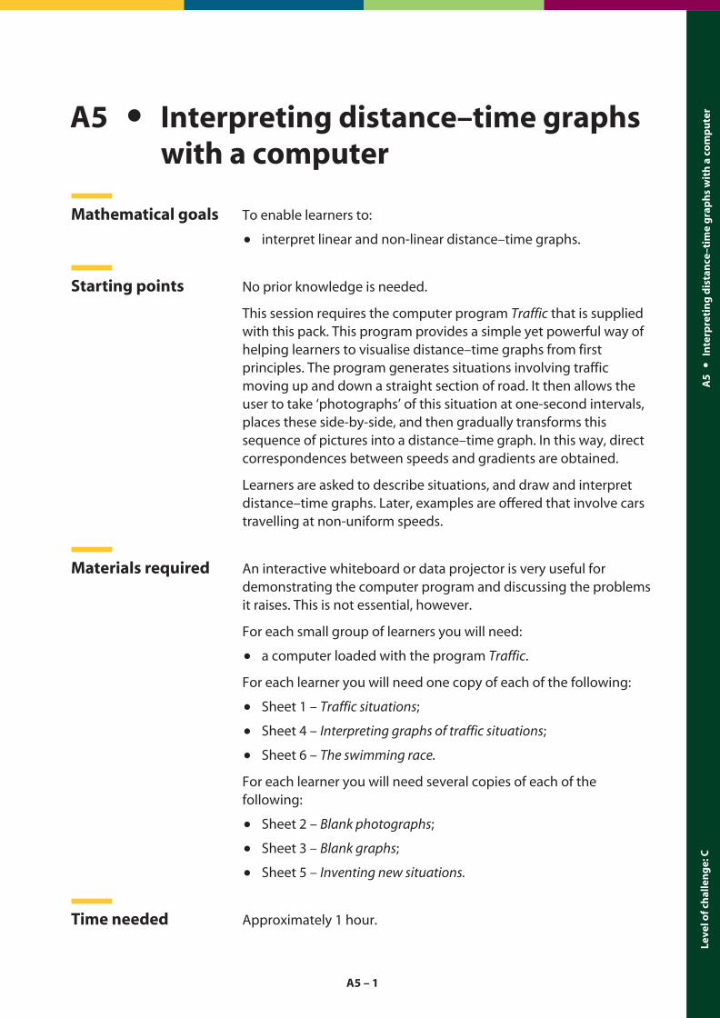
Now click ‘Options’ and tick the buttons marked ‘Photos’, ‘Markers’and ‘Graph’. Show the first few photographs of the situation, andclick ‘Pause’.

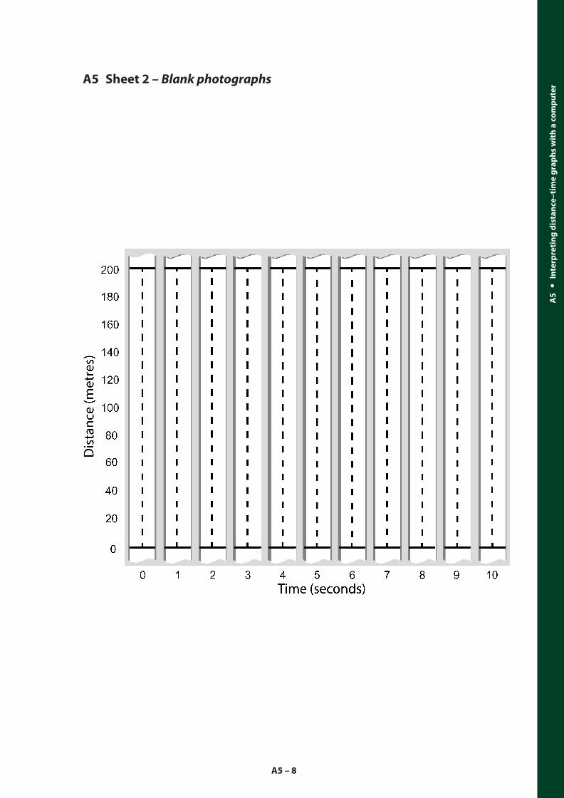
On the left hand side of the screen are photographs of thesituation taken at one second intervals. These are laid outside-by-side. Can you predict what the following photos willlook like?

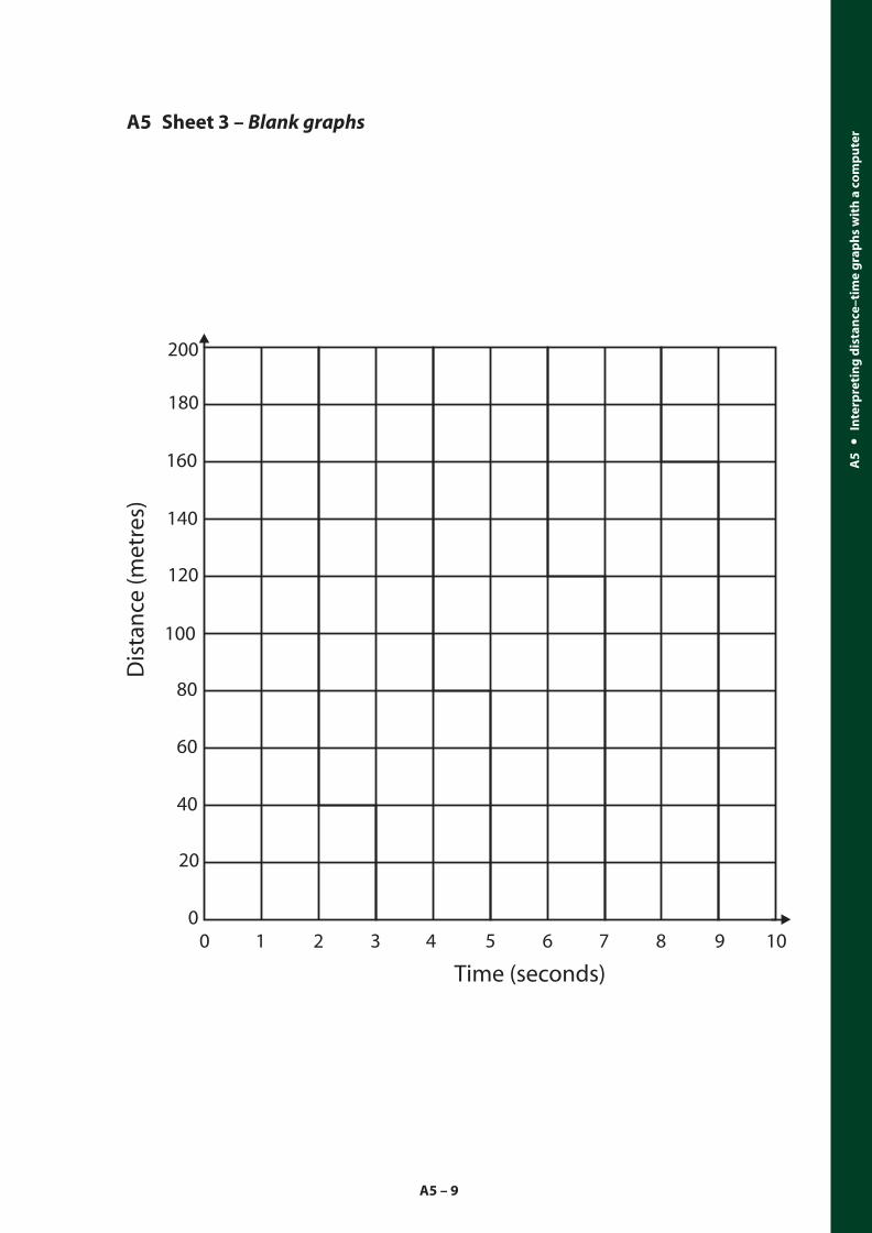
Hand out copies of Sheet 2 – Blank photographs and Sheet 3 – Blankgraphs and ask learners to fill in their second-by-second predictions.Now press ‘Play’ and ask learners to check whether their predictionswere correct.

From a set of photos, how can you tell that a vehicle isstationary? How can you tell that a vehicle is travellingquickly? How can you tell that it is travelling slowly?

A5 – 2

Leve

lofc

hal

len

ge:

CA

5In

terp

reti

ng

dis

tan

ce–t

ime

gra

ph

sw

ith

aco

mp

ute

r

What would the photos look like if we shot two photos persecond and laid them out side by side? 20 photos persecond?

The last question may be used to draw out the continuity of thesituation.

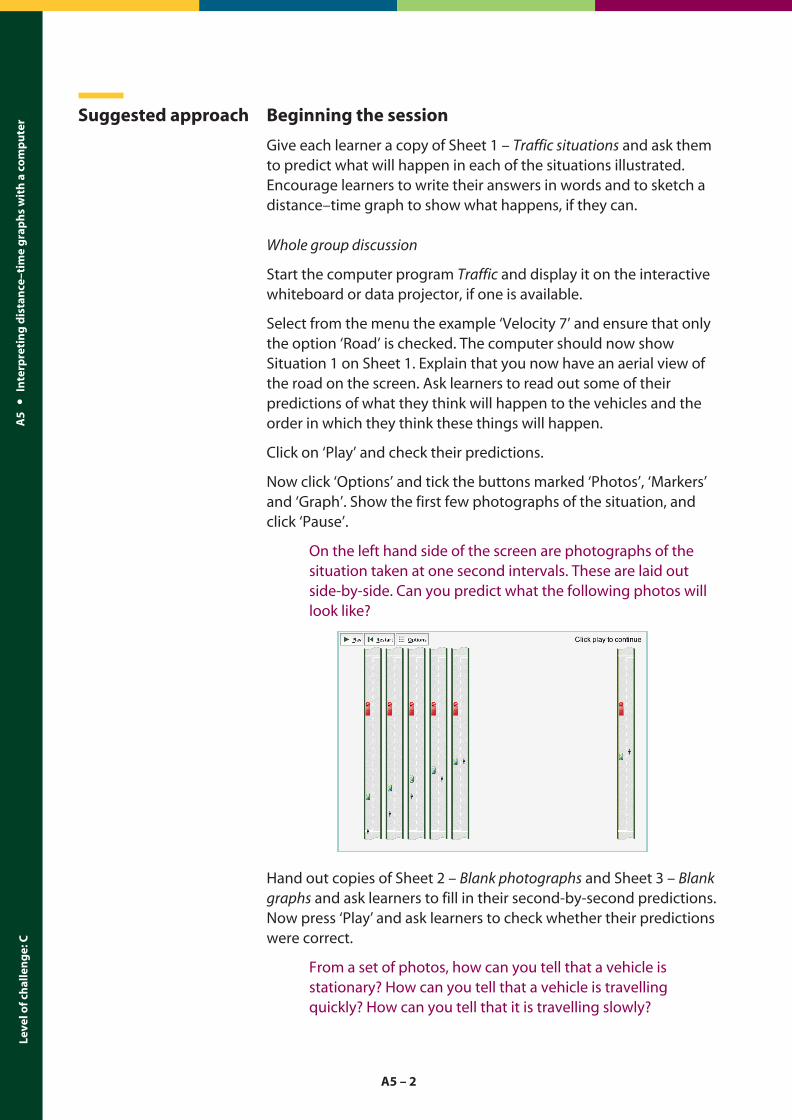
Explain that the photo predictions are a bit like a distance–timegraph of the situation. In a distance–time graph, we represent thesituation at each second using a vertical line, not by a picture of theroad. Click on ‘Play’ to show this transition.

Explain that a graph must also show scales. Click on ‘Play’ again toshow this.

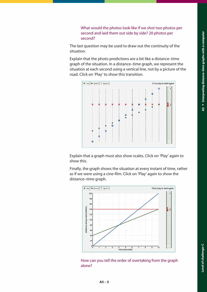
Finally, the graph shows the situation at every instant of time, ratheras if we were using a cine-film. Click on ‘Play’ again to show thedistance–time graph.

How can you tell the order of overtaking from the graphalone?

A5 – 3

Leve

lofc

hal

len

ge:

CA

5In

terp

reti

ng

dis

tan

ce–t

ime

gra

ph

sw

ith

aco

mp

ute

r

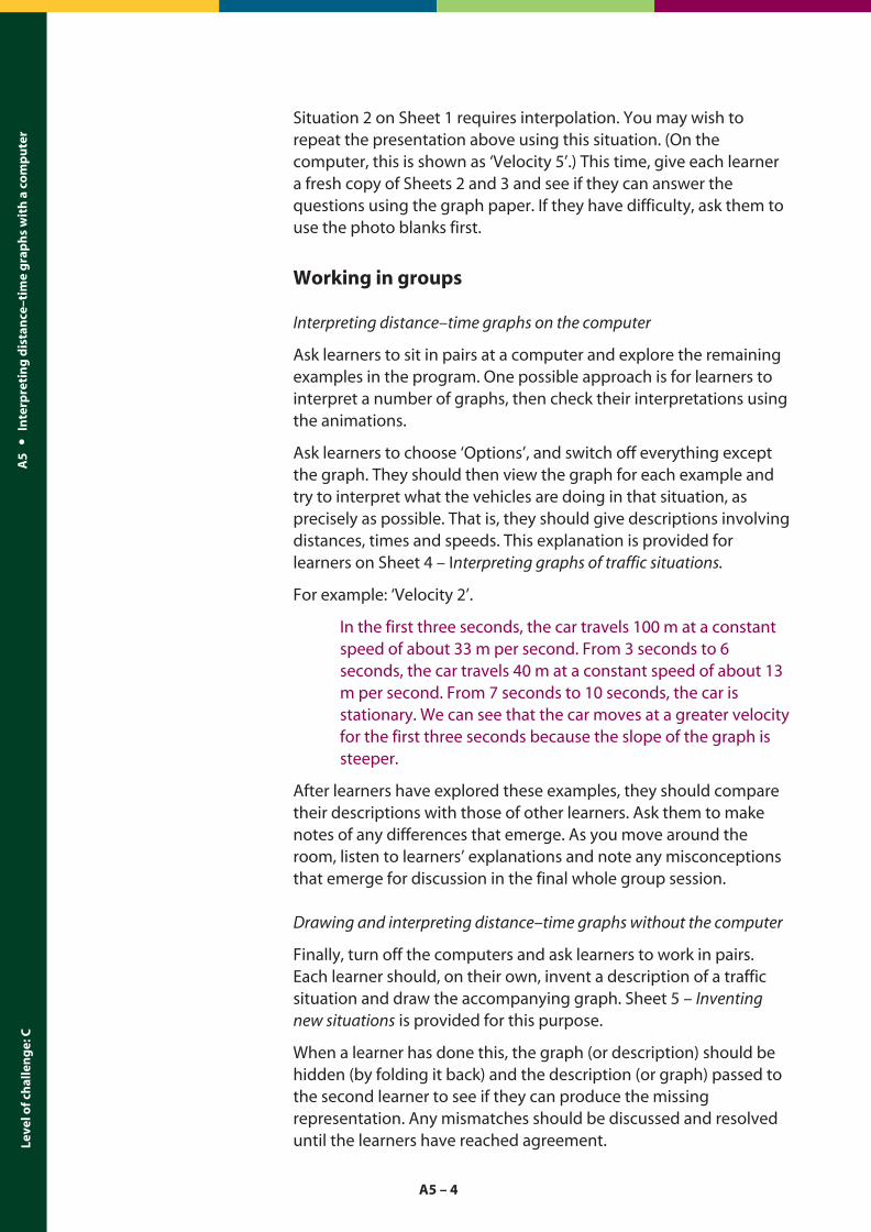
Situation 2 on Sheet 1 requires interpolation. You may wish torepeat the presentation above using this situation. (On thecomputer, this is shown as ‘Velocity 5’.) This time, give each learnera fresh copy of Sheets 2 and 3 and see if they can answer thequestions using the graph paper. If they have difficulty, ask them touse the photo blanks first.

Working in groups

Interpreting distance–time graphs on the computer

Ask learners to sit in pairs at a computer and explore the remainingexamples in the program. One possible approach is for learners tointerpret a number of graphs, then check their interpretations usingthe animations.

Ask learners to choose ‘Options’, and switch off everything exceptthe graph. They should then view the graph for each example andtry to interpret what the vehicles are doing in that situation, asprecisely as possible. That is, they should give descriptions involvingdistances, times and speeds. This explanation is provided forlearners on Sheet 4 – Interpreting graphs of traffic situations.

For example: ‘Velocity 2’.

In the first three seconds, the car travels 100 m at a constantspeed of about 33 m per second. From 3 seconds to 6seconds, the car travels 40 m at a constant speed of about 13m per second. From 7 seconds to 10 seconds, the car isstationary. We can see that the car moves at a greater velocityfor the first three seconds because the slope of the graph issteeper.

After learners have explored these examples, they should comparetheir descriptions with those of other learners. Ask them to makenotes of any differences that emerge. As you move around theroom, listen to learners’ explanations and note any misconceptionsthat emerge for discussion in the final whole group session.

Drawing and interpreting distance–time graphs without the computer

Finally, turn off the computers and ask learners to work in pairs.Each learner should, on their own, invent a description of a trafficsituation and draw the accompanying graph. Sheet 5 – Inventingnew situations is provided for this purpose.

When a learner has done this, the graph (or description) should behidden (by folding it back) and the description (or graph) passed tothe second learner to see if they can produce the missingrepresentation. Any mismatches should be discussed and resolveduntil the learners have reached agreement.

A5 – 4

Leve

lofc

hal

len

ge:

CA

5In

terp

reti

ng

dis

tan

ce–t

ime

gra

ph

sw

ith

aco

mp

ute

r

Reviewing and extending learning

Finally, hold a whole group discussion on the situation described inSheet 6 – The swimming race.

Give each learner a copy of Sheet 6 and read it together slowly. If alearner thinks that a mistake has been made, ask them to describethe mistake carefully and how it should be corrected.

What learnersmight do next

Learners may find A6 Interpreting distance–time graphs a usefulfollow-up to this session. This takes the ideas further and brings inthe measurement of acceleration and deceleration.

A5 – 5

Leve

lofc

hal

len

ge:

CA

5In

terp

reti

ng

dis

tan

ce–t

ime

gra

ph

sw

ith

aco

mp

ute

r

BLANK PAGE FOR NOTES

A5 – 6

Leve

lofc

hal

len

ge:

CA

5In

terp

reti

ng

dis

tan

ce–t

ime

gra

ph

sw

ith

aco

mp

ute

r

A5 – 7

A5

Inte

rpre

tin

gd

ista

nce

–tim

eg

rap

hs

wit

ha

com

pu

ter

A5 Sheet 1 – Traffic situations

40 m

100 m

20 m s–1

10 m s–1

Parked

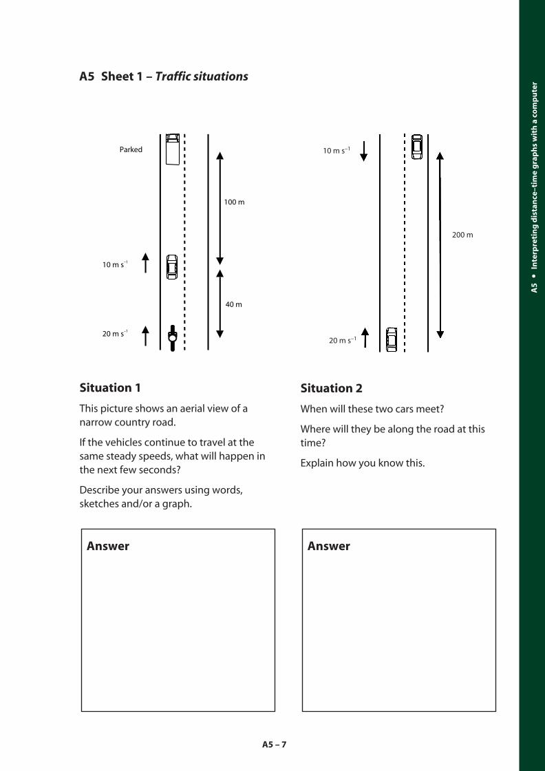
Situation 1

This picture shows an aerial view of anarrow country road.

If the vehicles continue to travel at thesame steady speeds, what will happen inthe next few seconds?

Describe your answers using words,sketches and/or a graph.

10 m s–1

20 m s–1

200 m

Situation 2

When will these two cars meet?

Where will they be along the road at thistime?

Explain how you know this.

Answer Answer

A5 – 8

A5

Inte

rpre

tin

gd

ista

nce

–tim

eg

rap

hs

wit

ha

com

pu

ter

A5 Sheet 2 – Blank photographs

A5 – 9

A5

Inte

rpre

tin

gd

ista

nce

–tim

eg

rap

hs

wit

ha

com

pu

ter

A5 Sheet 3 – Blank graphs

0 1 2 3 4 5 6 7 8 9 100

20

40

60

80

100

120

140

160

180

200

Time (seconds)

Dis

tan

ce (m

etre

s)

A5 – 10

A5

Inte

rpre

tin

gd

ista

nce

–tim

eg

rap

hs

wit

ha

com

pu

terA5 Sheet 4 – Interpreting graphs of traffic situations

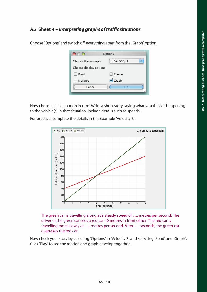
Choose ‘Options’ and switch off everything apart from the ‘Graph’ option.

Now choose each situation in turn. Write a short story saying what you think is happeningto the vehicle(s) in that situation. Include details such as speeds.

For practice, complete the details in this example ‘Velocity 3’.

The green car is travelling along at a steady speed of ...... metres per second. Thedriver of the green car sees a red car 40 metres in front of her. The red car istravelling more slowly at ...... metres per second. After ...... seconds, the green carovertakes the red car.

Now check your story by selecting ‘Options’ in ‘Velocity 3’ and selecting ‘Road’ and ‘Graph’.Click ‘Play’ to see the motion and graph develop together.

A5 – 11

A5

Inte

rpre

tin

gd

ista

nce

–tim

eg

rap

hs

wit

ha

com

pu

terA5 Sheet 5 – Inventing new situations

Description

. . . . . . . . . . . . . . . . . . . . . . . . . . . . . . . . . . . . . . . . . . . . . . . . . . . . . . . . . . .

. . . . . . . . . . . . . . . . . . . . . . . . . . . . . . . . . . . . . . . . . . . . . . . . . . . . . . . . . . .

. . . . . . . . . . . . . . . . . . . . . . . . . . . . . . . . . . . . . . . . . . . . . . . . . . . . . . . . . . .

. . . . . . . . . . . . . . . . . . . . . . . . . . . . . . . . . . . . . . . . . . . . . . . . . . . . . . . . . . .

. . . . . . . . . . . . . . . . . . . . . . . . . . . . . . . . . . . . . . . . . . . . . . . . . . . . . . . . . . .

. . . . . . . . . . . . . . . . . . . . . . . . . . . . . . . . . . . . . . . . . . . . . . . . . . . . . . . . . . .

. . . . . . . . . . . . . . . . . . . . . . . . . . . . . . . . . . . . . . . . . . . . . . . . . . . . . . . . . . .

. . . . . . . . . . . . . . . . . . . . . . . . . . . . . . . . . . . . . . . . . . . . . . . . . . . . . . . . . . .

. . . . . . . . . . . . . . . . . . . . . . . . . . . . . . . . . . . . . . . . . . . . . . . . . . . . . . . . . . .

. . . . . . . . . . . . . . . . . . . . . . . . . . . . . . . . . . . . . . . . . . . . . . . . . . . . . . . . . . .

. . . . . . . . . . . . . . . . . . . . . . . . . . . . . . . . . . . . . . . . . . . . . . . . . . . . . . . . . . .

. . . . . . . . . . . . . . . . . . . . . . . . . . . . . . . . . . . . . . . . . . . . . . . . . . . . . . . . . . .

Graph

0 1 2 3 4 5 6 7 8 9 100

20

40

60

80

100

120

140

160

180

200

Time (seconds)

Dis

tan

ce (m

etre

s)

A5 – 12

A5

Inte

rpre

tin

gd

ista

nce

–tim

eg

rap

hs

wit

ha

com

pu

ter

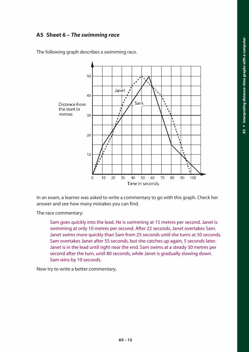
A5 Sheet 6 – The swimming race

The following graph describes a swimming race.

In an exam, a learner was asked to write a commentary to go with this graph. Check heranswer and see how many mistakes you can find.

The race commentary:

Sam goes quickly into the lead. He is swimming at 15 metres per second. Janet isswimming at only 10 metres per second. After 22 seconds, Janet overtakes Sam.Janet swims more quickly than Sam from 25 seconds until she turns at 50 seconds.Sam overtakes Janet after 55 seconds, but she catches up again, 5 seconds later.Janet is in the lead until right near the end. Sam swims at a steady 30 metres persecond after the turn, until 80 seconds, while Janet is gradually slowing down.Sam wins by 10 seconds.

Now try to write a better commentary.