Faculty of Engineering

Bachelor of Science in Computer Engineering

A WTA COMPETITIVE LEARNINGALGORITHM FOR THE

DEVELOPMENT OF CORTICALRECEPTIVE FIELDS

Thesis Supervisors:

Prof. M. C. CARROZZA

Prof. M. PAPPALARDO

Prof. G. VAGLINI

Author:

GIACOMO SPIGLER

December, 2012

1

COPYRIGHT c©

By

GIACOMO SPIGLER

December, 2012

ABSTRACT

This thesis investigates the problem of modeling the learning of cortical receptive

fields through competitive interaction mediated by local winner take all operations.

Given the great amount of data about the Primary Visual Cortex V1, such cortical

area is used for a meaningful comparison of the physiological responses and the shape

of the learnt receptive fields. The learning algorithm we developed is based on the

basic Oja learning rule, but convergence to different weight vectors is enforced by

local competition.

3

ACKNOWLEDGMENTS

I would like to thank all my friends, with whom I shared so many wonderful

experiences. A big thanks is deserved by Valerio, for the hilarious times he surely

remembers, by FruFFri (aka Francesca), for everything in the past three years, and

by Niccolo’, for the university and life experiences.

I am extremely grateful to Scuola Sant’Anna and all the people and friends I’ve

met there, who accompanied me in the past three years and with whom in those

years I shared most of my life. Another thanks goes to my high school professors at

Liceo Newton, who guided me through a personal growth and could appreciate my

proactivity.

The biggest thanks is for my parents, who always supported me and gave me

countless opportunities to travel, study and learn, and they taught me the value of

work and education.

Last but not least, I owe a special thanks to Dr. Calogero Oddo and Prof. Maria

Chiara Carrozza for their critical help in reviewing this Thesis.

Pisa, 26th November

iv

TABLE OF CONTENTS

Chapter Page

1 INTRODUCTION 1

2 BACKGROUND 2

2.1 Biology . . . . . . . . . . . . . . . . . . . . . . . . . . . . . . . . . . . . . . 2

2.1.1 Neurons . . . . . . . . . . . . . . . . . . . . . . . . . . . . . . . . . . 2

2.1.2 Neocortical architecture: layers, mini/macro columns . . . . . . . . . 4

2.1.3 Maps . . . . . . . . . . . . . . . . . . . . . . . . . . . . . . . . . . . 6

2.1.4 Visual System . . . . . . . . . . . . . . . . . . . . . . . . . . . . . . 8

2.2 Computation . . . . . . . . . . . . . . . . . . . . . . . . . . . . . . . . . . . 12

2.2.1 Hebbian Learning . . . . . . . . . . . . . . . . . . . . . . . . . . . . 12

2.2.2 HMAX . . . . . . . . . . . . . . . . . . . . . . . . . . . . . . . . . . 14

2.2.3 LISSOM . . . . . . . . . . . . . . . . . . . . . . . . . . . . . . . . . . 16

3 Cortical Learning 20

3.1 Methods . . . . . . . . . . . . . . . . . . . . . . . . . . . . . . . . . . . . . . 20

3.1.1 Input . . . . . . . . . . . . . . . . . . . . . . . . . . . . . . . . . . . 21

3.1.2 Activation . . . . . . . . . . . . . . . . . . . . . . . . . . . . . . . . . 22

3.1.3 Learning . . . . . . . . . . . . . . . . . . . . . . . . . . . . . . . . . . 23

3.2 Results . . . . . . . . . . . . . . . . . . . . . . . . . . . . . . . . . . . . . . . 24

4 DISCUSSION AND CONCLUSIONS 28

BIBLIOGRAPHY 29

A Simulations 34

v

CHAPTER 1

INTRODUCTION

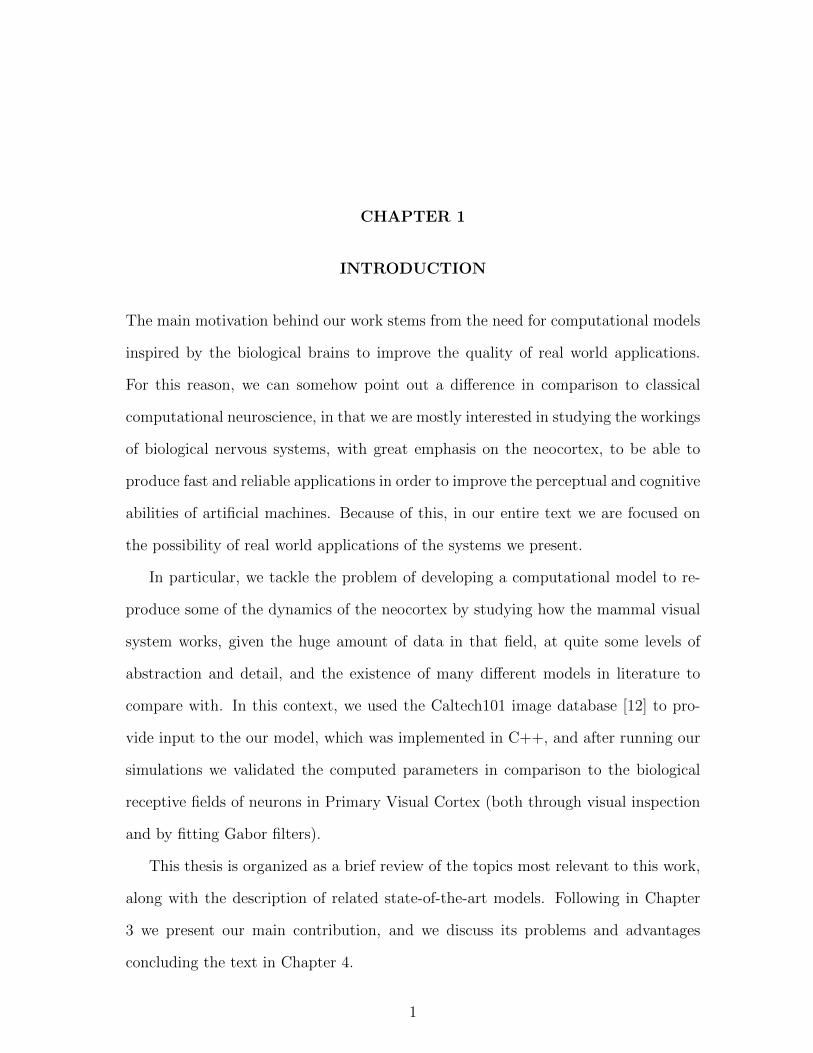
The main motivation behind our work stems from the need for computational models

inspired by the biological brains to improve the quality of real world applications.

For this reason, we can somehow point out a difference in comparison to classical

computational neuroscience, in that we are mostly interested in studying the workings

of biological nervous systems, with great emphasis on the neocortex, to be able to

produce fast and reliable applications in order to improve the perceptual and cognitive

abilities of artificial machines. Because of this, in our entire text we are focused on

the possibility of real world applications of the systems we present.

In particular, we tackle the problem of developing a computational model to re-

produce some of the dynamics of the neocortex by studying how the mammal visual

system works, given the huge amount of data in that field, at quite some levels of

abstraction and detail, and the existence of many different models in literature to

compare with. In this context, we used the Caltech101 image database [12] to pro-

vide input to the our model, which was implemented in C++, and after running our

simulations we validated the computed parameters in comparison to the biological

receptive fields of neurons in Primary Visual Cortex (both through visual inspection

and by fitting Gabor filters).

This thesis is organized as a brief review of the topics most relevant to this work,

along with the description of related state-of-the-art models. Following in Chapter

3 we present our main contribution, and we discuss its problems and advantages

concluding the text in Chapter 4.

1

CHAPTER 2

BACKGROUND

We begin with a quick review of the main concepts in neuroscience that are required

for the scope of this work, and we present some models which are the state of the art

of the problem being discussed.

2.1 Biology

In this brief summary, we begin from the most basic elements of biological Nervous

Systems, the neurons. We then identify more complex building blocks of the mam-

malian Neocortex, identifying its structure and elements. At last, we conclude with

a discussion about the (primate / mammal) Visual System and its parts which are

most relevant for this thesis, such as cortical maps and the Primary Visual Cortex.

2.1.1 Neurons

1Figure 2.1: A neuron

[19].

Neurons are the basic cellular elements of the nervous sys-

tem, and they are the main signaling units [19]. There have

been found many types of these highly specialized cells, but

all share a common morphology (see Fig. 2.1 for an exam-

ple). Despite some variability, neurons usually receive sig-

nals through their Dendrites, process information and pro-

duce an output, which is transmitted by their Axon as a

sequential membrane depolarization, the Action Potential.

2

Even though we don’t yet know all the mechanisms for neural coding of information,

several have been identified, ranging from Rate coding (frequency of spikes) to Tem-

poral coding (accounting for the precise timing at which spikes are generated) and to

Population coding (single neuron output is noisy, but the joint activity of a cluster

of cells can be very robust). Communication is mediated by electrochemical signals

in the Synapses, special structures connecting neurons (usually, axons to dendrites).

At the level of a synapse, action potentials cause the release of endogenous chemi-

cals, the Neurotransmitters, that in turn bind with specific Receptors, which control

the ion flux in the post-synaptic cell. Neurotransmitters can be Amino acids (eg,

glutamate, one of the most ubiquitous, present in excitatory synapses, and GABA γ-

aminobutyric acid, employed by inhibitory interneurons), Peptides or other chemicals

(eg, acetylcholine).

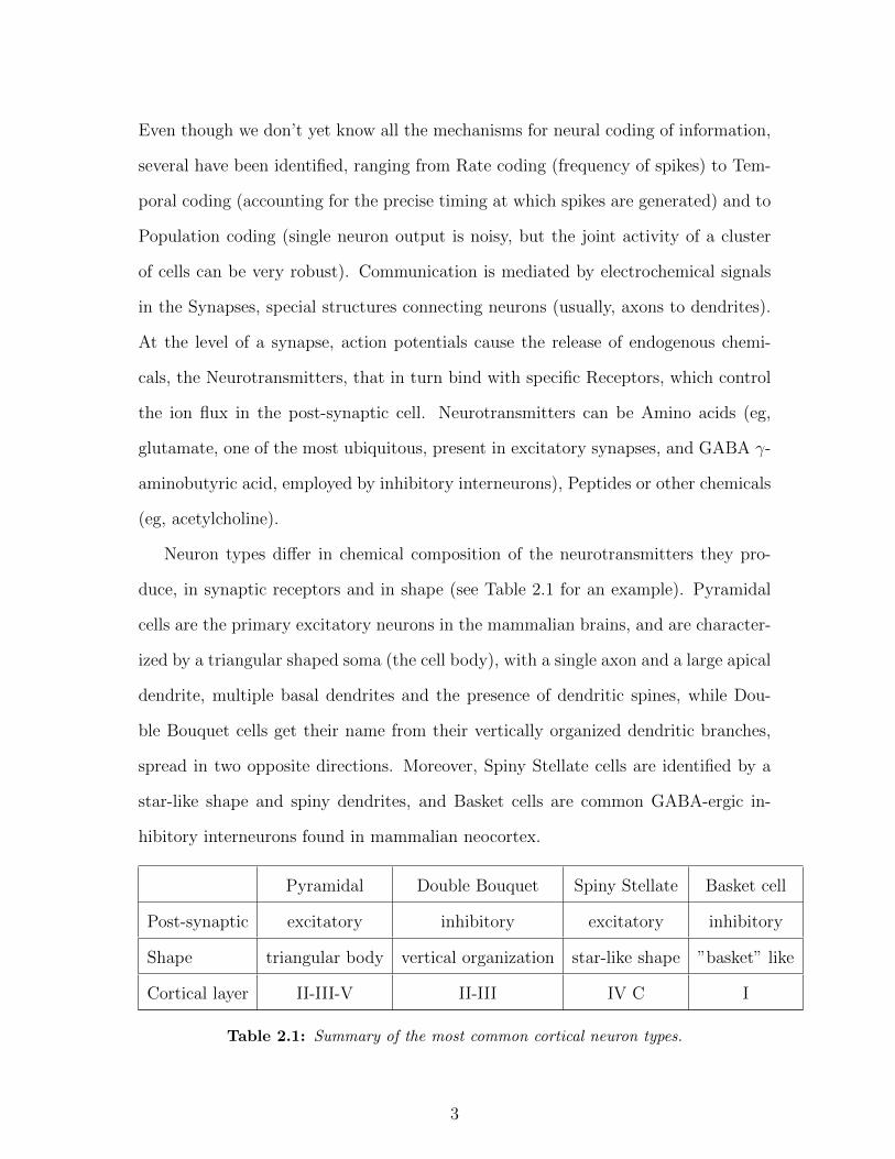
Neuron types differ in chemical composition of the neurotransmitters they pro-

duce, in synaptic receptors and in shape (see Table 2.1 for an example). Pyramidal

cells are the primary excitatory neurons in the mammalian brains, and are character-

ized by a triangular shaped soma (the cell body), with a single axon and a large apical

dendrite, multiple basal dendrites and the presence of dendritic spines, while Dou-

ble Bouquet cells get their name from their vertically organized dendritic branches,

spread in two opposite directions. Moreover, Spiny Stellate cells are identified by a

star-like shape and spiny dendrites, and Basket cells are common GABA-ergic in-

hibitory interneurons found in mammalian neocortex.

Pyramidal Double Bouquet Spiny Stellate Basket cell

Post-synaptic excitatory inhibitory excitatory inhibitory

Shape triangular body vertical organization star-like shape ”basket” like

Cortical layer II-III-V II-III IV C I

Table 2.1: Summary of the most common cortical neuron types.

3

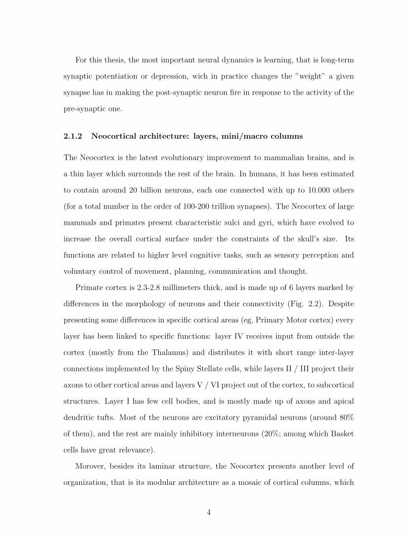
For this thesis, the most important neural dynamics is learning, that is long-term

synaptic potentiation or depression, wich in practice changes the ”weight” a given

synapse has in making the post-synaptic neuron fire in response to the activity of the

pre-synaptic one.

2.1.2 Neocortical architecture: layers, mini/macro columns

The Neocortex is the latest evolutionary improvement to mammalian brains, and is

a thin layer which surrounds the rest of the brain. In humans, it has been estimated

to contain around 20 billion neurons, each one connected with up to 10.000 others

(for a total number in the order of 100-200 trillion synapses). The Neocortex of large

mammals and primates present characteristic sulci and gyri, which have evolved to

increase the overall cortical surface under the constraints of the skull’s size. Its

functions are related to higher level cognitive tasks, such as sensory perception and

voluntary control of movement, planning, communication and thought.

Primate cortex is 2.3-2.8 millimeters thick, and is made up of 6 layers marked by

differences in the morphology of neurons and their connectivity (Fig. 2.2). Despite

presenting some differences in specific cortical areas (eg, Primary Motor cortex) every

layer has been linked to specific functions: layer IV receives input from outside the

cortex (mostly from the Thalamus) and distributes it with short range inter-layer

connections implemented by the Spiny Stellate cells, while layers II / III project their

axons to other cortical areas and layers V / VI project out of the cortex, to subcortical

structures. Layer I has few cell bodies, and is mostly made up of axons and apical

dendritic tufts. Most of the neurons are excitatory pyramidal neurons (around 80%

of them), and the rest are mainly inhibitory interneurons (20%; among which Basket

cells have great relevance).

Morover, besides its laminar structure, the Neocortex presents another level of

organization, that is its modular architecture as a mosaic of cortical columns, which

4

Figure 2.2: Laminar structure of the Neocortex.

have been proposed as the basic building blocks of cortical function [26] [7]. In fact,

experiments proved that neurons aligned perpendicularly to the surface of the cortex

and within a diameter of 28-40 um responded to stimuli in a very similar way, whereas

the response was quite different moving tangentially. Each minicolumn contains 80-

120 neurons on average, and is highly interconnected with neighboring columns. Also,

these structures can be further grouped into macrocolumns, being modules inside

which a full set of values for any set of receptive field parameters is found (eg, in

Hubel and Wiesel IceCube model of V1, a macrocolumn contains columns selective

to a full range of orientations and spatial frequencies, for both eyes). Some estimates

suggest there are 50-100 minicolumns composing each macrocolumn, for a total of

4000-12000 neurons and a diameter of 200-800 um. Neurons farther apart than this

length don’t generally have overlapping receptive fields.

After first discovery of the cortical minicolumn in the 50s [25] a lot of research

5

provided evidence in support of a broad columnar organization across the cortex,

with special mention deserved for sensory cortices [18] [10] [11], motor cortex, IT

(Infero-Temporal) [37] and PFC (PreFrontal Cortex) [26].

2.1.3 Maps

There is evidence that cortical columns are arranged in a smooth, locally continuous

way, relative to their preferred stimuli.

The most striking examples of such organization came from the study of the

Primary Visual Cortex V1 and Somatosensory / Motor Cortices. V1 maps have been

studied extensively ([8] for a review, along with the original contributions by Hubel

and Wiesel), and are organized in a retinotopic way, with a superposition of maps

representing the same modality, such as ocular dominance, orientation (see Fig. 2.3),

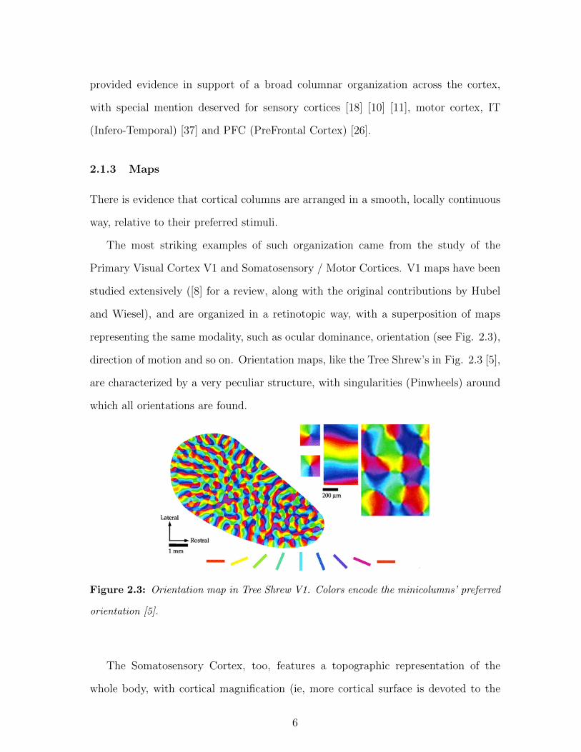
direction of motion and so on. Orientation maps, like the Tree Shrew’s in Fig. 2.3 [5],

are characterized by a very peculiar structure, with singularities (Pinwheels) around

which all orientations are found.

Figure 2.3: Orientation map in Tree Shrew V1. Colors encode the minicolumns’ preferred

orientation [5].

The Somatosensory Cortex, too, features a topographic representation of the

whole body, with cortical magnification (ie, more cortical surface is devoted to the

6

representation of some parts of the body, like hands and face, than it would in relation

to their real proportions). The so-called sensory and motor Homunculi are shown in

Fig. 2.4.

Figure 2.4: Sensory (left) and Motor (right) homunculi.

Different models have been proposed to explain the observed structures, with the

most biological being the effect of recurrent dynamics of lateral connections [22].

Alternative works try to explain the phenomenon by moire interference of almost

regularly spaced ON- and OFF-center Retinal Ganglion Cells [29] (in relation to

visual maps) or by means of a geometric interpretation [30]. Another interesting

approach was undertaken by Rojer and Schwartz [32] [34], who observed that simply

smoothing a random pattern of orientations (represented as unit amplitude complex

numbers) leads to the appearance of orientation maps organized in close resemblance

to the biological counterparts, and justified the finding as a topological result (non-

retraction of R2 → S1). The result holds for a map or randomly arranged Gabor

filters (ie, a cortical lattice where each unit’s receptive field is a randomly oriented

Gabor filter), as well.

7

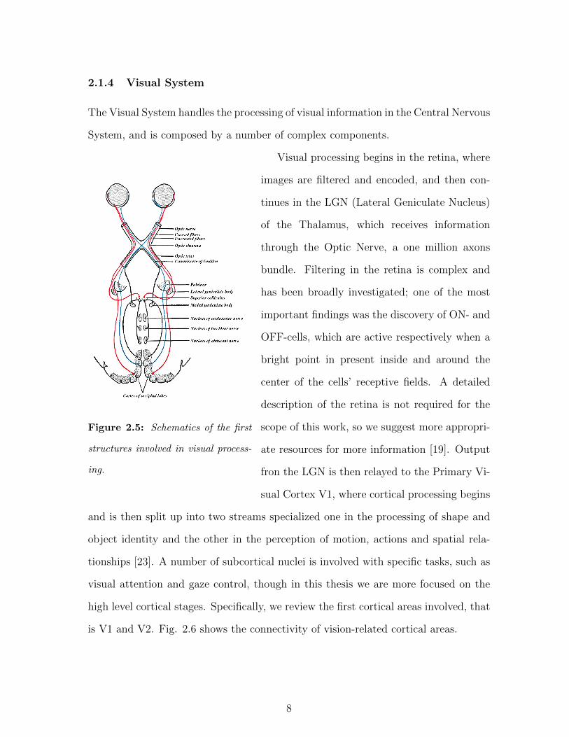
2.1.4 Visual System

The Visual System handles the processing of visual information in the Central Nervous

System, and is composed by a number of complex components.

Figure 2.5: Schematics of the first

structures involved in visual process-

ing.

Visual processing begins in the retina, where

images are filtered and encoded, and then con-

tinues in the LGN (Lateral Geniculate Nucleus)

of the Thalamus, which receives information

through the Optic Nerve, a one million axons

bundle. Filtering in the retina is complex and

has been broadly investigated; one of the most

important findings was the discovery of ON- and

OFF-cells, which are active respectively when a

bright point in present inside and around the

center of the cells’ receptive fields. A detailed

description of the retina is not required for the

scope of this work, so we suggest more appropri-

ate resources for more information [19]. Output

fron the LGN is then relayed to the Primary Vi-

sual Cortex V1, where cortical processing begins

and is then split up into two streams specialized one in the processing of shape and

object identity and the other in the perception of motion, actions and spatial rela-

tionships [23]. A number of subcortical nuclei is involved with specific tasks, such as

visual attention and gaze control, though in this thesis we are more focused on the

high level cortical stages. Specifically, we review the first cortical areas involved, that

is V1 and V2. Fig. 2.6 shows the connectivity of vision-related cortical areas.

8

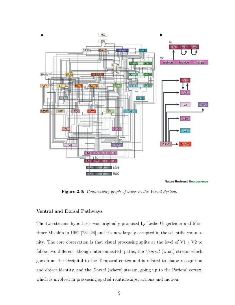
Figure 2.6: Connectivity graph of areas in the Visual System.

Ventral and Dorsal Pathways

The two-streams hypothesis was originally proposed by Leslie Ungerleider and Mor-

timer Mishkin in 1982 [23] [24] and it’s now largely accepted in the scientific commu-

nity. The core observation is that visual processing splits at the level of V1 / V2 to

follow two different -though interconnected- paths, the Ventral (what) stream which

goes from the Occipital to the Temporal cortex and is related to shape recognition

and object identity, and the Dorsal (where) stream, going up to the Parietal cortex,

which is involved in processing spatial relationships, actions and motion.

9

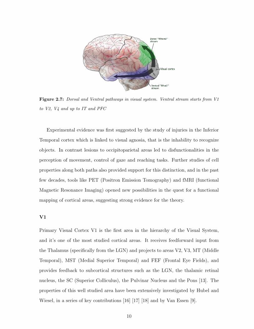
Figure 2.7: Dorsal and Ventral pathways in visual system. Ventral stream starts from V1

to V2, V4 and up to IT and PFC

Experimental evidence was first suggested by the study of injuries in the Inferior

Temporal cortex which is linked to visual agnosia, that is the inhability to recognize

objects. In contrast lesions to occipitoparietal areas led to disfunctionalities in the

perception of movement, control of gaze and reaching tasks. Further studies of cell

properties along both paths also provided support for this distinction, and in the past

few decades, tools like PET (Positron Emission Tomography) and fMRI (functional

Magnetic Resonance Imaging) opened new possibilities in the quest for a functional

mapping of cortical areas, suggesting strong evidence for the theory.

V1

Primary Visual Cortex V1 is the first area in the hierarchy of the Visual System,

and it’s one of the most studied cortical areas. It receives feedforward input from

the Thalamus (specifically from the LGN) and projects to areas V2, V3, MT (Middle

Temporal), MST (Medial Superior Temporal) and FEF (Frontal Eye Fields), and

provides feedback to subcortical structures such as the LGN, the thalamic retinal

nucleus, the SC (Superior Colliculus), the Pulvinar Nucleus and the Pons [13]. The

properties of this well studied area have been extensively investigated by Hubel and

Wiesel, in a series of key contributions [16] [17] [18] and by Van Essen [9].

10

Functionally, V1 shows retinotopy (ie, neighboring points on the retina map to

neighboring positions in the cortex) and contains a complete map of the visual field.

Moreover, the retinal image is distorted so that the central part corresponding to

the Fovea -the central 2% of the image- covers 50% of the cortical surface. It has

been estimated that V1 is composed of around 140 million neurons per hemisphere

in humans, and has an average surface of 25-30 cm2 [20].

Figure 2.8: Response of Simple and

Complex cells in V1. Complex cells

fire whenever their preferred stimulus

is present, whereas Simple cells only

fire when it is present at a definite

position.

Neurons in V1 are selective to a set of fea-

tures, like oriented lines, spatial frequency, di-

rection of motion, temporal frequency, dispar-

ity (and ocular dominance) and color (through

color-opponent units). Their receptive fields are

precisely localized and they are about 0.5 - 2 de-

grees in size near the fovea. A special mention

goes to orientation selective cells, because of the

extensive research and amount of data (both in

terms of single-unit and map organization stud-

ies). A striking feature of these cells is their divi-

sion between Simple and Complex cells, with the

first being selective to specifically oriented bars

at definite positions inside their receptive field,

and the others producing a sustained response

whenever the preferred stimulus is present, with

local invariance to its position. A schematic of

this difference is shown in Fig. 2.8, which plots the spiking activity of ideal Simple

and Complex cells tuned to vertical bars.

11

2.2 Computation

The computational background is mostly based on the well estabilished Hebbian

theory of synaptic plasticity. Morover, we present three models at different levels

of detail, that is Unit (representing cortical columns) through Hebbian Learning,

Maps with lateral interaction and System by taking advantage of higher level features

of cortical processing, such as the building of invariant representations of external

stimuli.

2.2.1 Hebbian Learning

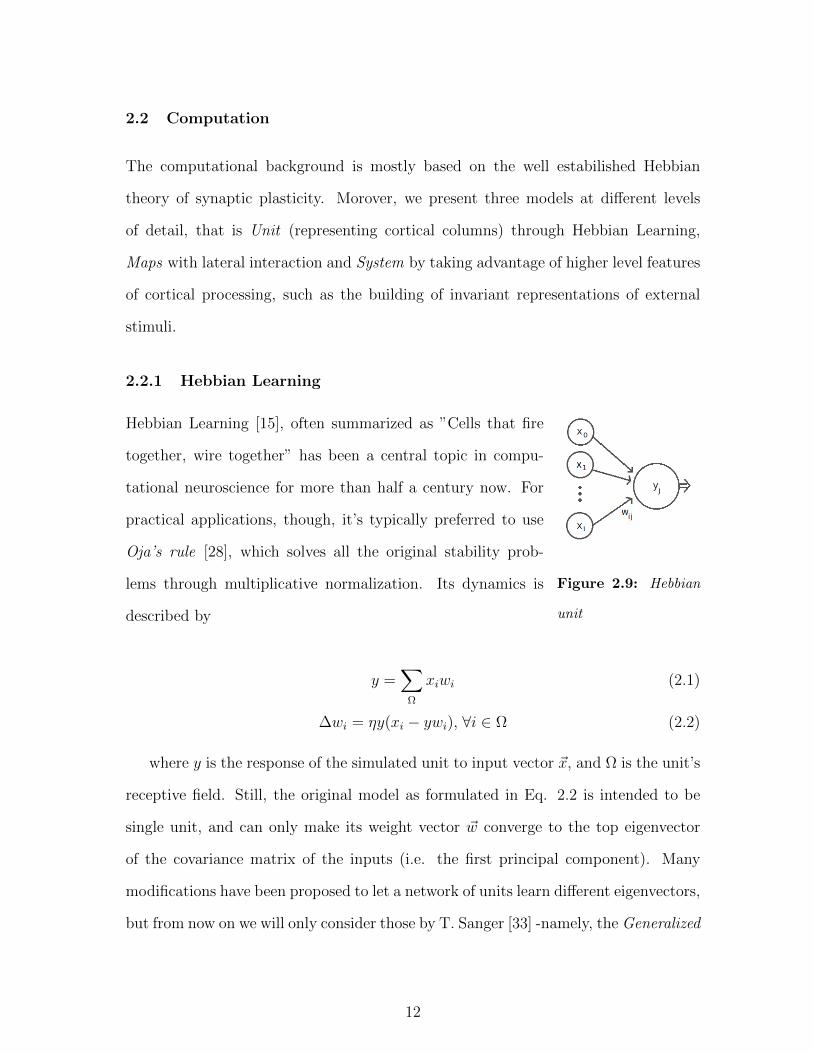
Figure 2.9: Hebbian

unit

Hebbian Learning [15], often summarized as ”Cells that fire

together, wire together” has been a central topic in compu-

tational neuroscience for more than half a century now. For

practical applications, though, it’s typically preferred to use

Oja’s rule [28], which solves all the original stability prob-

lems through multiplicative normalization. Its dynamics is

described by

y =∑

Ω

xiwi (2.1)

∆wi = ηy(xi − ywi), ∀i ∈ Ω (2.2)

where y is the response of the simulated unit to input vector ~x, and Ω is the unit’s

receptive field. Still, the original model as formulated in Eq. 2.2 is intended to be

single unit, and can only make its weight vector ~w converge to the top eigenvector

of the covariance matrix of the inputs (i.e. the first principal component). Many

modifications have been proposed to let a network of units learn different eigenvectors,

but from now on we will only consider those by T. Sanger [33] -namely, the Generalized

12

Hebbian Algorithm, GHA-, which combine Oja’s rule with the Gram-Schmidt process

∆wij = ηyj(xi −j∑

k=0

ykwik) (2.3)

with wij repesenting the strength of the connection between the i-th afferent input

and the j-th unit. It has been shown that Eq. 2.3 with p units makes the weights to

converge to the first p principal components of the inputs [33]. An example of weights

after convergence is shown in Fig. 2.10.

Figure 2.10: 30 weights corresponding to the first 30 Principal Components of images of

oriented gaussians. Weights were learnt according to Eq. 2.3 with specific simulations in

the context of this thesis.

However, we are more interested in sampling a bigger variety of the top compo-

nents, rather than computing a full PCA. For instance, with reference to Fig. 2.10,

we might want to make the units’ weights converge to a bigger variety of orientations

(like the 2nd and 3rd units from the left)

Another set of simulations was run by masking (i.e., multiplying) the input re-

ceptive field with a Gaussian filter, to better model the localization of the receptive

fields, rather than just hard-limiting them. An example of such a simulation is shown

in Fig. 2.11.

Figure 2.11: Weights computed as in Fig. 2.10, representing the top Principal Components

of uniformly translating natural images, seen through a gaussian aperture with σ = 6.

13

Hebbian learning is also used to solve different problems, by setting the appropri-

ate constraints. It has been used to perform ICA (Independent Components Analysis)

[14] by implementing lateral inhibitory connections updated with the so-called Anti-

Hebbian rule, that is

∆wij = −ηyiyj (2.4)

More generally, we always need some kind of Competition between the Hebbian

units to force their weights to converge to different vectors. Common algorithms are

WTA (Winner Take All), k-WTA, SotMAX or sparseness constraints, like in [38].

2.2.2 HMAX

HMAX is a biologically motivated framework, based on a quantitative theory of the

organization of the ventral stream of the visual system [36] [35] [27], which addresses

the problem of how visual cortex recognizes objects.

Specifically, the system models the first hundreds of milliseconds of feedforward

cortical processing since the presentation of a new image, in order to avoid interference

from feedback connections.

The model is based on the construction of an increasingly invariant representation

of features, by alternating stages of template matching and spatial pooling across a

hierarchy of processing layers. Higher stages in the hierarchy also correspond to higher

features’ complexity and bigger receptive fields, similar to the biological counterpart.

In its basic form, the model is made up of 4 layers, where S ”Simple cells” layers

(S1 and S2) alternate with C ”Complex cells” layers (C1 and C2), implementing

respectively the feature matching and the pooling operations, as in Figure 2.12.

Pre-processing : the image to be processed is first used to build a gaussian pyramid

(eg, 10 scales, each one a factor 4√

2 smaller than the last [27])

S1 : S1 layer takes the pyramid as input, and convolves every scaled image with

a set of Ng Gabor filters (similar to V1 Simple Cells tuned to gabor-like stimuli),

14

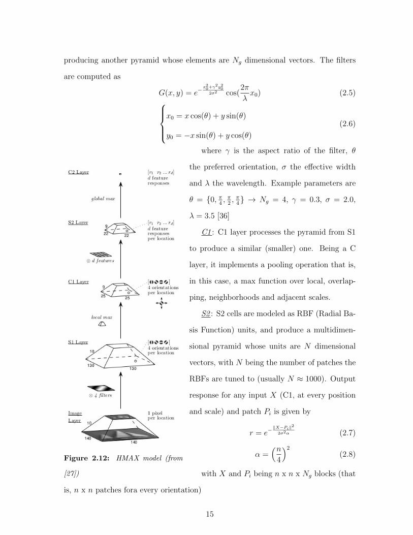
producing another pyramid whose elements are Ng dimensional vectors. The filters

are computed as

G(x, y) = e−x20+γ

2y202σ2 cos(

2π

λx0) (2.5)

x0 = x cos(θ) + y sin(θ)

y0 = −x sin(θ) + y cos(θ)

(2.6)

Figure 2.12: HMAX model (from

[27])

where γ is the aspect ratio of the filter, θ

the preferred orientation, σ the effective width

and λ the wavelength. Example parameters are

θ = 0, π4, π

2, π

4 → Ng = 4, γ = 0.3, σ = 2.0,

λ = 3.5 [36]

C1 : C1 layer processes the pyramid from S1

to produce a similar (smaller) one. Being a C

layer, it implements a pooling operation that is,

in this case, a max function over local, overlap-

ping, neighborhoods and adjacent scales.

S2 : S2 cells are modeled as RBF (Radial Ba-

sis Function) units, and produce a multidimen-

sional pyramid whose units are N dimensional

vectors, with N being the number of patches the

RBFs are tuned to (usually N ≈ 1000). Output

response for any input X (C1, at every position

and scale) and patch Pi is given by

r = e−‖X−Pi‖

2

2σ2α (2.7)

α =(n

4

)2

(2.8)

with X and Pi being n x n x Ng blocks (that

is, n x n patches fora every orientation)

15

C2 : The last layer implements a global pooling, and outputs a N -dimensional

vector, whose elements are the maximum over every position and scale for each S2

patch.

Learning : Learning in the model occurs in S2 layer, and is performed by collecting

a number of C1 patches at random positions, scales and sizes (n = 4, 8, 12, 16),

with a score function (eg, energy) to select the most discriminative ones. It has been

tested both extracting C1 patches over all the orientations [35] and in a sparse fashion,

selecting the dominant one for all the element of the patches [27].

Classification: even though the output from the model is represented by the C2

responses, higher level classification for object recognition is usually performed by

training a linear classifier such as SVM (Support Vector Machine) on the output

vector. For a comparison of performance in reference to other systems we suggest

[35] [27].

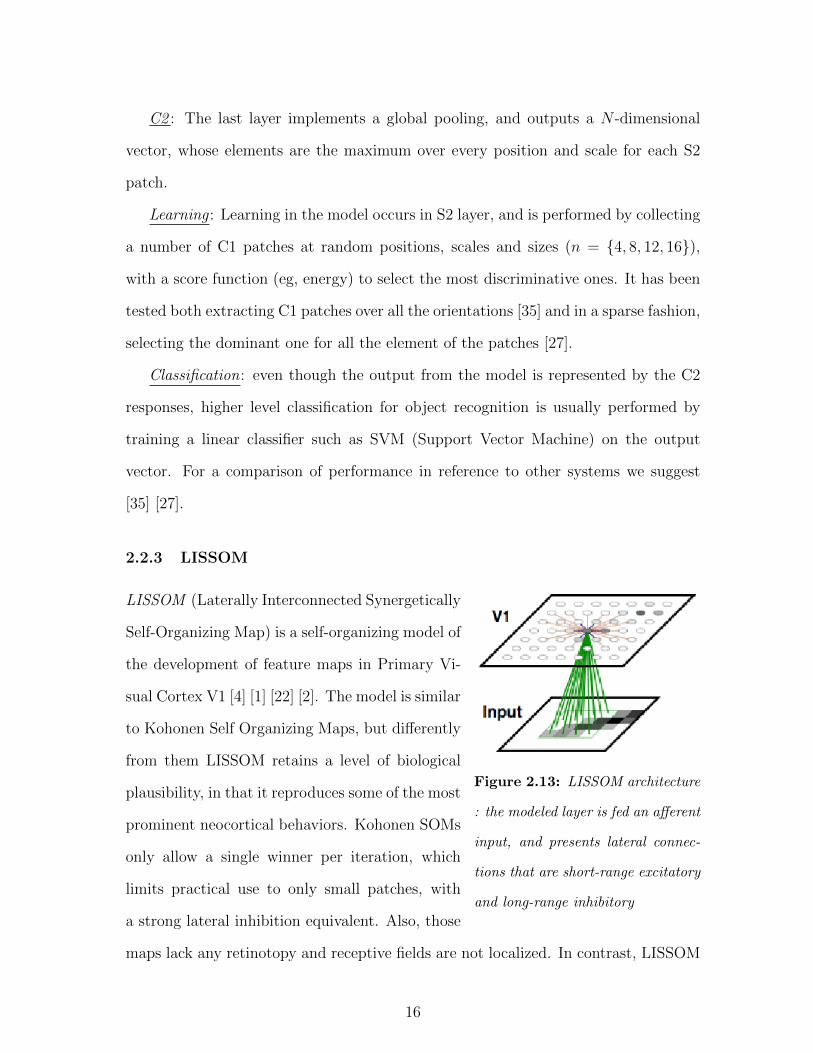
2.2.3 LISSOM

Figure 2.13: LISSOM architecture

: the modeled layer is fed an afferent

input, and presents lateral connec-

tions that are short-range excitatory

and long-range inhibitory

LISSOM (Laterally Interconnected Synergetically

Self-Organizing Map) is a self-organizing model of

the development of feature maps in Primary Vi-

sual Cortex V1 [4] [1] [22] [2]. The model is similar

to Kohonen Self Organizing Maps, but differently

from them LISSOM retains a level of biological

plausibility, in that it reproduces some of the most

prominent neocortical behaviors. Kohonen SOMs

only allow a single winner per iteration, which

limits practical use to only small patches, with

a strong lateral inhibition equivalent. Also, those

maps lack any retinotopy and receptive fields are not localized. In contrast, LISSOM

16

employs recurrent lateral interactions -which are learnt at run-time- to sharpen ac-

tivity around strongly activated spots (multiple local winners occur at the same time,

instead of a global winner). Moreover, activaton is computed as a function of dot

product between the afferent input, localized retinotopically, and the unit’s weights

(rather than computing their euclidean distance). Currently the model (GCAL, gain-

control adaptive laterally connected) also features mechanisms for automatic homeo-

static plasticity in place of the activation thresholds, and gain control to remove local

contrast in the input [3] [39].

In practice, LISSOM is implemented as a layer made up of processing units. The

layer is fed another layer as input (eg, an image, representing a ”retina”, or another

layer [31]), and specifically, every unit has an afferent receptive field localized in the

corresponding position of the input layer (ie, retinotopically). The Computation of

the activation of the units requires two steps: computing the raw output, and settling

activation with recurrent interaction from lateral connections. At the first step we

compute the initial activation ζj of unit j

ζj =∑

i∈Afferentj

xiwij (2.9)

with x being the input and w being the afferent weights linking input unit i to

layer unit j. We can then compute the final activation by letting lateral connection

reach an equilibrium

yj(t) = σ

ζj + γE∑

i∈excj

wEiyi(t− 1)− γI∑

i∈inhj

wIiyi(t− 1)

(2.10)

σ(x) =

0 x ≤ δ

x−δβ−δ δ < x < β

1 x ≥ β

(2.11)

17

where yj(t) is the output of unit j at step t (recurrent iterations are simulated for

T times, eg T = 10), wEi and wIi are the strenghts of the lateral connections. σ(x)

is a piece-wise approximation of the sigmoidal function, and it models threshold /

saturation phenomena.

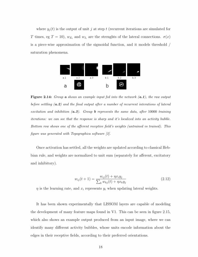
Figure 2.14: Group a shows an example input fed into the network (a.1), the raw output

before settling (a.2) and the final output after a number of recurrent interations of lateral

excitation and inhibition (a.3). Group b represents the same data, after 10000 training

iterations: we can see that the response is sharp and it’s localized into an activity bubble.

Bottom row shows one of the afferent receptive field’s weights (untrained vs trained). This

figure was generated with Topographica software [2].

Once activation has settled, all the weights are updated according to classical Heb-

bian rule, and weights are normalized to unit sum (separately for afferent, excitatory

and inhibitory).

wij(t+ 1) =wij(t) + ηxiyj∑k wkj(t) + ηxkyj

(2.12)

η is the learning rate, and xi represents yi when updating lateral weights.

It has been shown experimentally that LISSOM layers are capable of modeling

the development of many feature maps found in V1. This can be seen in figure 2.15,

which also shows an example output produced from an input image, where we can

identify many different activity bubbles, whose units encode information about the

edges in their receptive fields, according to their preferred orientations.

18

Figure 2.15: Left is a trained LISSOM layer whose units have been color-coded to represent

their preferred orientation. Right is the output of the trained layer when presented the retinal

image (a). (b) shows the LGN-filtered image, which is fed into the layer, while the bottom

row contains three different outputs of the layer, under different gain-contrast settings (color

coded for the units’ preferred orientations). Like Fig. 2.14, this figure was generated with

Topographica software [2].

19

CHAPTER 3

Cortical Learning

Now that we have reviewed the background of this research we can outline the core

topic. The problem we face is part of the broader task of developing a computational

model of the Neocortex, and is motivated by the relative lack of fast algorithms to

simulate the development of cortical receptive fields. Morover, we want to develop a

model inspired by the biological system, but targeted for applications, for instance in

humanoid robotics and computer vision.

Now, the first property we want the system to have is full unsupervised learning

of the units’ weights, possibly with a stable output representation computed using

them, and given as a 2D activity map. Also, we would expect the final receptive fields

to be sparse and in close resemblance to those identified in V1, ie, Gabor filters.

3.1 Methods

We choose to model a 2D patch of a neural layer, whose units represent overall activity

of cortical minicolumns. Every unit is associated with an afferent weight matrix to

model its receptive field, and a specific position in the input map (correspondent

to its position in the layer). Minicolumns are grouped into non-overlapping square

clusters to approximante the local dynamics of macrocolumns. We decided to model

the Primary Visual Cortex, so the input is passed through a very basic model of

processing in the Retina+LGN. A picture of the system is shown in Fig. 3.1. Also,

computational complexity was considered, in that we wanted it not to be greater than

20

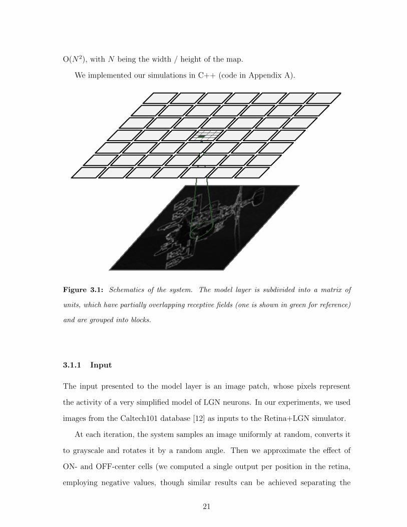
O(N2), with N being the width / height of the map.

We implemented our simulations in C++ (code in Appendix A).

Figure 3.1: Schematics of the system. The model layer is subdivided into a matrix of

units, which have partially overlapping receptive fields (one is shown in green for reference)

and are grouped into blocks.

3.1.1 Input

The input presented to the model layer is an image patch, whose pixels represent

the activity of a very simplified model of LGN neurons. In our experiments, we used

images from the Caltech101 database [12] as inputs to the Retina+LGN simulator.

At each iteration, the system samples an image uniformly at random, converts it

to grayscale and rotates it by a random angle. Then we approximate the effect of

ON- and OFF-center cells (we computed a single output per position in the retina,

employing negative values, though similar results can be achieved separating the

21

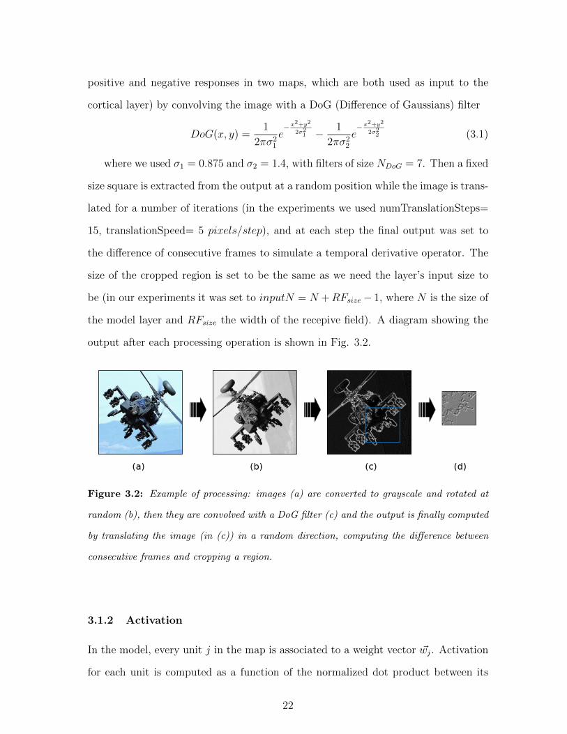
positive and negative responses in two maps, which are both used as input to the

cortical layer) by convolving the image with a DoG (Difference of Gaussians) filter

DoG(x, y) =1

2πσ21

e−x

2+y2

2σ21 − 1

2πσ22

e−x

2+y2

2σ22 (3.1)

where we used σ1 = 0.875 and σ2 = 1.4, with filters of size NDoG = 7. Then a fixed

size square is extracted from the output at a random position while the image is trans-

lated for a number of iterations (in the experiments we used numTranslationSteps=

15, translationSpeed= 5 pixels/step), and at each step the final output was set to

the difference of consecutive frames to simulate a temporal derivative operator. The

size of the cropped region is set to be the same as we need the layer’s input size to

be (in our experiments it was set to inputN = N +RFsize− 1, where N is the size of

the model layer and RFsize the width of the recepive field). A diagram showing the

output after each processing operation is shown in Fig. 3.2.

Figure 3.2: Example of processing: images (a) are converted to grayscale and rotated at

random (b), then they are convolved with a DoG filter (c) and the output is finally computed

by translating the image (in (c)) in a random direction, computing the difference between

consecutive frames and cropping a region.

3.1.2 Activation

In the model, every unit j in the map is associated to a weight vector ~wj. Activation

for each unit is computed as a function of the normalized dot product between its

22

weight and the portion of the input which falls under its receptive field ~x.

yj =~wj · ~x‖~wj‖‖~x‖

(3.2)

yj = f(yj) (3.3)

where yj is the output of layer unit j, and f is a function which can be used

to introduce non-linearities in the activation. In the experiments we show in this

thesis, we always used the identity function f(x) = x. Also, in some tests, we forced

the receptive field to be in a Gaussian envelope, which seems a more natural way to

localize the RFs than just truncating the input outside the units’ preferred positions

in the retina. In practice, we multiplied the input vector with a Gaussian mask

xi = G(i)xi (3.4)

where G(i) is the Gaussian mask centered on the unit’s receptive field with a fixed

σx.

3.1.3 Learning

The main part of the model is the learning algorithm, which controls how the units’

weights are updated at each iteration. The rule is based on Competitive Learning,

mediated by a hard WTA (Winner Take All) local to each macrocolumn, and extends

the Oja’s Rule [28] [21].

Specifically, we first compute the maximum activation for each macrocolumn Mk

Zk = maxj∈Mk

yj (3.5)

then, we update the weights of all the units in the macrocolumn according to

∆wij = ηyj(xi − yjwij) (3.6)

where η = η0 (in our experiments η0 = 0.007) for yj = Zk, and η = −η0/100 ∀yj < Zk.

Learning rate η0 is fixed during all the simulation.

23

3.2 Results

We run our simulations for 100.000 iterations (though good convergence was reached

after the first tens of thousands) over a range of parameters. All the plots presented

in this section were either computed as 2x2 or 6x6 matrices of macrocolumns (for

plotting purpose only), each one composed by 4x4 units, and receptive field size was

set to RFsize = 13, unless otherwise stated. The pictures show the learnt weights of

each unit, grouped per block, and converted to gray scale images, where light gray

represents zero and brigher/darker shades stand for positive and negative values,

respectively.

• Learning of weights with basic settings (Fig. 3.3)

The first set of simulations were tested in relation to the change of different pa-

rameters, such as learning rate and size of modules and receptive fields. Inputs

were patches processed like described in Section 3.1.1.

• A smaller map developed like first, but showing the units’ weights in greater

detail (Fig. 3.4)

For ease of presentation we also trained a small layer, to show the weights after

development with better clarity. Fig. 3.4 highlights the fine, smooth details of

the orientation tuning.

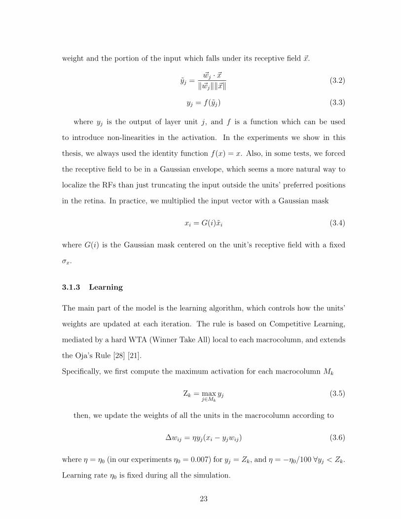
• Weights were trained on inputs masked with a Gaussian filter (Fig. 3.5)

Another set of simulations was run by multiplying the units’ receptive fields

with a Gaussian mask, to provide a smoother localization function. Most of the

weights after convergence closely remind of Gabor filters.

24

Figure 3.3: Converged weights of 6x6 modules (macrocolumns), each composed by 4x4

units (minicolumns) with no gaussian aperture. RFsize = 13, that is the filters are 13x13

in size.

Figure 3.4: Like Fig. 3.3 with 2x2 macrocolumns.

25

Figure 3.5: Like Fig. 3.3 but with inputs multiplied by a gaussian filter with σ = 6.

As we can see, weights after convergence show a preference for specifically oriented

lines, which is compatible with other models of V1 and with experimental physiolog-

ical evidence. To further explore this result, we fitted the weights in Fig. 3.4 with 2D

Gabor filters (Eq. 2.5), computing the parameters which made them most similar.

For ease of computation, we manually set most of the values, which were constant

for all the weights, and we optimized for orientation θ and position (x0, y0). Fig. 3.6

shows an example of such reconstruction, along with the Gabor parameters used to

generate the filters. A broader view is shown in Fig. 3.7, featuring the full matrix of

reconstructed weights.

26

(a) (b) (c)

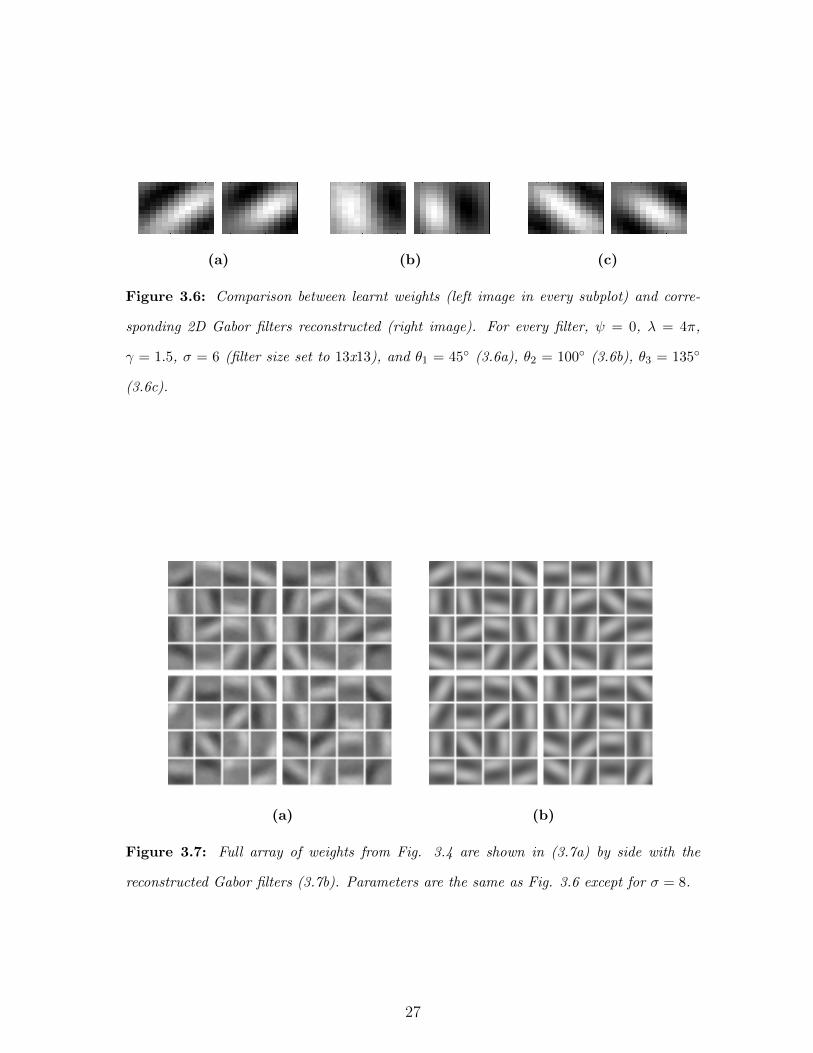
Figure 3.6: Comparison between learnt weights (left image in every subplot) and corre-

sponding 2D Gabor filters reconstructed (right image). For every filter, ψ = 0, λ = 4π,

γ = 1.5, σ = 6 (filter size set to 13x13), and θ1 = 45 (3.6a), θ2 = 100 (3.6b), θ3 = 135

(3.6c).

(a) (b)

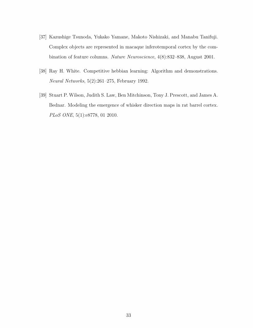
Figure 3.7: Full array of weights from Fig. 3.4 are shown in (3.7a) by side with the

reconstructed Gabor filters (3.7b). Parameters are the same as Fig. 3.6 except for σ = 8.

27

CHAPTER 4

DISCUSSION AND CONCLUSIONS

As we can see from the plots in section 3.2 all the units but a little number develop

orientation selectivity by looking at translating images, and they show interesting

features changing the main parameters.

Future work will be focused primarily on the use of Competitive Learning algo-

rithms like ours in learning multi-stage cortical weights in hierarchies, with special

interest in the mechanisms underlying the increase in invariance and, in this context,

the development of the receptive fields of Complex Cells. We are also going to vali-

date our system using inputs from different modalities or with bigger dimensionality

incorporating, for instance, binocularity and color representation, speaking about the

visual system. Last but not least, we will research the relation between our learning

algorithm and the formation of cortical maps, with the possible introduction of some

kind of local correlation, which would model the dynamics of short-range excitatory

synapses between minicolumns.

In conclusion, results look promising, and they suggest that the most basic prop-

erties of cortical response could be modeled with computationally friendly operations,

such as the Winner Take All. In this regard, the system we presented could be used

in computer vision applications and possibly in other machine learning applications,

as well.

28

BIBLIOGRAPHY

[1] Jan Antolik and James A Bednar. Development of maps of simple and complex

cells in the primary visual cortex. Frontiers in Computational Neuroscience,

5(17), 2011.

[2] James A Bednar. Topographica: building and analyzing map-level simulations

from python, c/c++, matlab, nest, or neuron components. Frontiers in Neu-

roinformatics, 3(8), 2009.

[3] James A. Bednar. Building a mechanistic model of the development and function

of the primary visual cortex. Journal of Physiology-Paris, (0), 2012.

[4] James A. Bednar and Risto Miikkulainen. Tilt aftereffects in a self-organizing

model of the primary visual cortex. Neural Computation, 12:1721–1740, 2000.

[5] William H. Bosking, Ying Zhang, Brett Schofield, and David Fitzpatrick. Ori-

entation selectivity and the arrangement of horizontal connections in tree shrew

striate cortex. The Journal of Neuroscience, 17(6):2112–2127, 1997.

[6] Gary Bradski. The OpenCV Library. Dr. Dobb’s Journal of Software Tools,

2000.

[7] Manuel F. Casanova. Neocortical Modularity and the Cell Minicolumn. 2005.

[8] Bruce M. Dow. Orientation and color columns in monkey visual cortex. Cerebral

Cortex, 12(10):1005–1015, 2002.

29

[9] David C. Van Essen and Charles H. Anderson. Information processing strategies

and pathways in the primate visual system. An Introduction to Neural and

Electronic Networks, pages 45–76, 1995.

[10] Oleg Favorov and Barry L. Whitsel. Spatial organization of the peripheral input

to area 1 cell columns. i. the detection of ’segregates’. Brain Research Reviews,

13(1):25 – 42, 1988.

[11] Oleg V. Favorov and Mathew E. Diamond. Demonstration of discrete place-

defined columnssegregatesin the cat si. The Journal of Comparative Neurology,

298(1):97–112, 1990.

[12] Li Fei-Fei, Rob Fergus, and Pietro Perona. Learning generative visual models

from few training examples: An incremental bayesian approach tested on 101

object categories. 2004.

[13] Daniel J. Felleman and David C. Van Essen. Distributed hierarchical processing

in the primate cerebral cortex. Cerebral Cortex, 1(1):1–47, 1991.

[14] Peter Foldiak. Forming sparse representations by local anti-hebbian learning.

Biological Cybernetics, 64:165–170, 1990.

[15] Donald O. Hebb. The organization of behavior. 1949.

[16] D. H. Hubel and T. N. Wiesel. Receptive fields, binocular interaction and

functional architecture in the cat’s visual cortex. The Journal of Physiology,

160(1):106–154, 1962.

[17] D. H. Hubel and T. N. Wiesel. Receptive fields and functional architecture of

monkey striate cortex. The Journal of Physiology, 195(1):215–243, 1968.

30

[18] David H. Hubel and Torsten N. Wiesel. Sequence regularity and geometry of

orientation columns in monkey striate cortex. Journal of Comparative Neurology,

158(3):267–294, 1974.

[19] Eric R. Kandel, James H. Schwartz, and Thomas M. Jessell. Principles of Neural

Science. 2000.

[20] G. Leuba and R. Kraftsik. Changes in volume, surface estimate, three-

dimensional shape and total number of neurons of the human primary visual

cortex from midgestation until old age. Anatomy and Embryology, 190:351 –

366, 1994.

[21] Timothee Masquelier, Thomas Serre, Simon Thorpe, and Tomaso Poggio. Learn-

ing complex cell invariance from natural videos: A plausibility proof. Technical

report, MIT, CSAIL, CBCL, 12 2007.

[22] Risto Miikkulainen, James A. Bednar, Yoonsuck Choe, and Joseph Sirosh. Com-

putational Maps in the Visual Cortex. Springer, 2005.

[23] Mortimer Mishkin and Leslie G. Ungerleider. Contribution of striate inputs to

the visuospatial functions of parieto-preoccipital cortex in monkeys. Behavioural

Brain Research, 6(1):57 – 77, 1982.

[24] Mortimer Mishkin, Leslie G. Ungerleider, and Kathleen A. Macko. Object vision

and spatial vision: two cortical pathways. Trends in Neurosciences, 6(0):414 –

417, 1983.

[25] Vernon B. Mountcastle. Modality and topographic properties of single neurons

of cat’s somatic sensory cortex. Journal of Neurophysiology, 20(4):408–434, 1957.

[26] Vernon B. Mountcastle. The columnar organization of the neocortex. Brain,

120(4):701–722, 1997.

31

[27] Jim Mutch and David G. Lowe. Object class recognition and localization using

sparse features with limited receptive fields. International Journal of Computer

Vision (IJCV), 80(1):45–57, October 2008.

[28] Erkki Oja. Simplified neuron model as a principal component analyzer. Journal

of Mathematical Biology, 15(3), 1982.

[29] Se-Bum Paik and Dario L. Ringach. Retinal origin of orientation maps in visual

cortex. Nat Neurosci, 14(7):919–925, Jul 2011.

[30] Jean Petitot. The neurogeometry of pinwheels as a sub-riemannian contact struc-

ture. Journal of Physiology-Paris, 97(23):265 – 309, 2003.

[31] Alessio Plebe and Rosaria Grazia Domenella. Early development of visual recog-

nition. Biosystems, 86(13):63 – 74, 2006.

[32] Alan S. Rojer and Eric L. Schwartz. Cat and monkey cortical columnar patterns

modeled by bandpass filtered 2d white noise. Biological Cybernetics, 62(5), 1990.

[33] Terence D. Sanger. Optimal unsupervised learning in a single-layer linear feed-

forward neural network. Neural Networks, 2(6), 1989.

[34] Eric L. Schwartz and Alan S. Rojer. Cortical hypercolumns and the topology of

random orientation maps. Pattern Recognition, 1994.

[35] Thomas Serre, Lior Wolf, Stan Bileschi, Maximilian Riesenhuber, and Tomaso

Poggio. Robust object recognition with cortex-like mechanisms. Pattern Analysis

and Machine Intelligence, IEEE Transactions on, 29(3):411 –426, march 2007.

[36] Thomas Serre, Lior Wolf, and Tomaso Poggio. Object recognition with features

inspired by visual cortex. 2:994 – 1000 vol. 2, june 2005.

32

[37] Kazushige Tsunoda, Yukako Yamane, Makoto Nishizaki, and Manabu Tanifuji.

Complex objects are represented in macaque inferotemporal cortex by the com-

bination of feature columns. Nature Neuroscience, 4(8):832–838, August 2001.

[38] Ray H. White. Competitive hebbian learning: Algorithm and demonstrations.

Neural Networks, 5(2):261–275, February 1992.

[39] Stuart P. Wilson, Judith S. Law, Ben Mitchinson, Tony J. Prescott, and James A.

Bednar. Modeling the emergence of whisker direction maps in rat barrel cortex.

PLoS ONE, 5(1):e8778, 01 2010.

33

APPENDIX A

Simulations

Following is the code used to run the simulations described in Chapter 3. The algo-

rithms described are implemented by the Retina and the Layer classes:

• Retina takes care of processing input images as described in 3.1.1

• Layer provides support for management of data structures required by the

model, and implements the learning algorithm in 3.1.3 (as well as computing

output activation as in 3.1.2)

The software requires linking with the OpenCV computer vision library [6].

1 #inc lude <s t d i o . h>

#inc lude <s t d l i b . h>

#inc lude <time . h>

#inc lude <math . h>

#inc lude <vector>

#inc lude <algor ithm>

#inc lude <cv . h>

#inc lude <highgu i . h>

11 #inc lude <iostream>

us ing namespace std ;

#de f i n e RETINAMODEDEBUG 0

#de f i n e RETINA MODE VIDEO 1

34

#de f i n e RETINAMODECALTECH 2

#de f i n e w r i t e i n t ( a , f p ) fw r i t e (&a , s i z e o f ( i n t ) , 1 , f p ) ;

#de f i n e w r i t e f l o a t ( a , f p ) fw r i t e (&a , s i z e o f ( f l o a t ) , 1 , f p ) ;

21 #de f i n e r ead in t ( a , f p ) f r ead (&a , s i z e o f ( i n t ) , 1 , f p ) ;

#de f i n e r e ad f l o a t ( a , f p ) f r ead (&a , s i z e o f ( f l o a t ) , 1 , f p ) ;

// F i r s t Stage o f p r o c e s s i ng

c l a s s Retina

pub l i c :

i n t width , he ight ;

i n t videoW , videoH ;

CvCapture ∗ capture ;

31 IplImage ∗prev , ∗cur , ∗tmp , ∗g1 , ∗g2 ;

IplImage ∗ image ;

i n t mode ;

i n t c a l t e ch r , ca l t e ch x , ca l t e ch y , c a l t e c h i i i ;

f l o a t c a l t e ch the t a , r o t a t e t h e t a ;

Retina ( i n t w, i n t h , i n t mode =RETINA MODE VIDEO) ;

41 ˜Retina ( ) ;

void getImage ( ) ;

;

35

// Second stage o f p r o c e s s i ng

c l a s s Layer

pub l i c :

51 i n t width , he ight ;

Retina ∗ r e t i n a ;

i n t r f , r f21 , r f 2 ;

f l o a t sigmaRf , sigmaRf2 ;

f l o a t ∗ gauss ianAperture ;

i n t moduleN , numModulesW , numModulesH ;

f l o a t ∗∗weights ;

f l o a t ∗out ;

61 f l o a t ∗ out exp ;

Layer ( i n t w, i n t h , i n t r f , i n t moduleN , f l o a t sigmaRf , Retina ∗ r ) ;

˜Layer ( ) ;

void save ( const char ∗ f i l e ) ;

Layer ( const char ∗ f i l e , Retina ∗ r ) ;

void t r a i n ( i n t numIterat ions ) ;

71 void getAl lWeights ( IplImage ∗weights out , f l o a t amp=1.0 f ) ;

;

Retina : : Retina ( i n t w, i n t h , i n t mode )

th i s−>width = w;

th i s−>he ight = h ;

36

th i s−>mode = mode ;

81

i f (mode ==RETINA MODE VIDEO)

th i s−>capture = cvCreateFi leCapture ( ” . . / ShowVideo . av i ” ) ;

IplImage ∗ frame=NULL;

whi l e ( ! frame )

frame=cvQueryFrame ( capture ) ;

th i s−>videoW = frame−>width ;

th i s−>videoH = frame−>he ight ;

91 th i s−>prev = cvCreateImage ( cvS i ze ( frame−>width , frame−>he ight ) ,

IPL DEPTH 8U , 1) ;

th i s−>cur = cvCreateImage ( cvS i ze ( frame−>width , frame−>he ight ) ,

IPL DEPTH 8U , 1) ;

cvZero ( th i s−>cur ) ;

th i s−>tmp = cvCreateImage ( cvS i z e ( frame−>width , frame−>he ight ) ,

IPL DEPTH 8U , 1) ;

th i s−>g1 = cvCreateImage ( cvS i ze ( frame−>width , frame−>he ight ) ,

IPL DEPTH 8U , 1) ;

th i s−>g2 = cvCreateImage ( cvS i ze ( frame−>width , frame−>he ight ) ,

IPL DEPTH 8U , 1) ;

th i s−>c a l t e c h i i i =0;

101 e l s e i f (mode ==RETINAMODECALTECH)

th i s−>tmp = cvCreateImage ( cvS i z e (w, h) , IPL DEPTH 8U , 1) ;

th i s−>g1 = cvCreateImage ( cvS i ze (w, h) , IPL DEPTH 8U , 1) ;

th i s−>g2 = cvCreateImage ( cvS i ze (w, h) , IPL DEPTH 8U , 1) ;

th i s−>c a l t e c h i i i =0;

37

th i s−>image = cvCreateImage ( cvS i z e (w, h) , IPL DEPTH 32F , 1) ;

111

Retina : : ˜ Retina ( )

cvReleaseCapture(&capture ) ;

cvReleaseImage(&prev ) ;

cvReleaseImage(&cur ) ;

cvReleaseImage(&tmp) ;

121 cvReleaseImage(&g1 ) ;

cvReleaseImage(&g2 ) ;

// U t i l i t y func t i on : draws a randomly o r i en t ed e longated gauss ian in to ”

im” image

void RandomGaussian ( IplImage ∗im , i n t cente red=0, f l o a t thr =0.369 f )

const i n t border=4;

131 const f l o a t a2=56.25;

const f l o a t b2=2.25;

i n t xc=( i n t ) ( ( f l o a t ) rand ( ) /( f l o a t (RANDMAX)+1.0) ∗( f l o a t ) ( im−>width−2∗

border ) )+border ;

i n t yc=( i n t ) ( ( f l o a t ) rand ( ) /( f l o a t (RANDMAX)+1.0) ∗( f l o a t ) ( im−>height−2∗

border ) )+border ;

38

i n t the ta =( i n t ) ( ( f l o a t ) rand ( ) /( f l o a t (RANDMAX)+1.0) ∗180 .0 ) ;

th e ta =the ta /15 ;

th e ta =the ta ∗15 ;

f l o a t theta=( f l o a t ) the ta /180 .0 ∗ 3 . 141592 ;

141

f l o a t co s t=cos ( theta ) ;

f l o a t s i n t=s i n ( theta ) ;

i f ( cente red==1)

xc=im−>width /2 ;

yc=im−>he ight /2 ;

151 f l o a t ∗ imf=( f l o a t ∗) im−>imageData ;

i n t p=im−>widthStep/ s i z e o f ( f l o a t ) ;

f o r ( i n t x=0; x<im−>width ; x++) f o r ( i n t y=0; y<im−>he ight ; y++)

i n t j=x−xc ;

i n t k=y−yc ;

f l o a t r e s=exp ( −( j ∗ co s t − k∗ s i n t ) ∗( j ∗ co s t − k∗ s i n t ) /a2 −( j ∗ s i n t + k∗

co s t ) ∗

( j ∗ s i n t + k∗ co s t ) /b2 ) ;

i f ( res>=thr ) imf [ y∗p+x]= r e s ;

161 e l s e imf [ y∗p+x ]=0 . 0 ;

39

// Main func t i on f o r ”Retina ” ob j e c t s : generate and proce s s input images

void Retina : : getImage ( )

const f l o a t SIGMA OUT = 1.4 f ;

const f l o a t SIGMA IN = 0.875 f ;

171

i f (mode==RETINAMODEDEBUG)

// Generate o r i en t ed gaus s i an s

RandomGaussian ( image , 0) ; // cente red

e l s e i f (mode==RETINAMODECALTECH)

// Process Caltech101 image

i n t sz = image−>width ;

i n t maxTransl=15;

181

i f ( ( c a l t e c h i i i%maxTransl )==0)

c a l t e c h r = ( i n t ) ( ( f l o a t ) rand ( ) / ( ( f l o a t )RANDMAX+1.0 f ) ∗9196.0 f )

;

char s t r [ 8 0 ] ; s p r i n t f ( s t r , ” . . / Caltech101/%d . png” , c a l t e c h r ) ;

IplImage ∗tmp = cvLoadImage ( s t r ) ;

i f ( ! tmp )

cout<<s t r<<endl ;

191

IplImage ∗tmp = cvCreateImage ( cvS i z e ( tmp −>width , tmp −>he ight ) ,

IPL DEPTH 8U , 1) ;

cvConvertImage ( tmp , tmp) ;

i n t mult=5;

40

i f ( ( c a l t e c h i i i%maxTransl )==0)

c a l t e ch x = ( i n t ) ( ( f l o a t ) rand ( ) / ( ( f l o a t )RANDMAX+1.0 f ) ∗(tmp−>

width−sz−2−2∗mult∗maxTransl ) )+1+mult∗maxTransl ;

c a l t e ch y = ( i n t ) ( ( f l o a t ) rand ( ) / ( ( f l o a t )RANDMAX+1.0 f ) ∗(tmp−>

height−sz−2−2∗mult∗maxTransl ) )+1+mult∗maxTransl ;

201 i n t the ta =( i n t ) ( ( f l o a t ) rand ( ) /( f l o a t (RANDMAX)+1.0) ∗360 .0 ) ;

th e ta =the ta /15 ;

th e ta =the ta ∗15 ;

c a l t e c h t h e t a=( f l o a t ) the ta /180 .0 ∗ 3 . 141592 ;

// theta =1.54 f ;

th e ta =( i n t ) ( ( f l o a t ) rand ( ) /( f l o a t (RANDMAX)+1.0) ∗360 .0 ) ;

th e ta =the ta /15 ;

th e ta =the ta ∗15 ;

r o t a t e t h e t a=( f l o a t ) the ta /180 .0 ∗ 3 . 141592 ;

211

IplImage ∗tmp2 = cvCreateImage ( cvS i z e ( tmp −>width , tmp −>he ight ) ,

IPL DEPTH 8U , 1) ;

f l o a t ang le = r o t a t e t h e t a ; // c a l t e c h t h e t a ;

f l o a t m[ 6 ] ;

CvMat M = cvMat (2 , 3 , CV 32F , m) ;

221

m[ 0 ] = ( f l o a t ) cos ( angle −3.141592 f /2 .0 f ) ;

m[ 1 ] = ( f l o a t ) s i n ( angle −3.141592 f /2 .0 f ) ;

m[ 3 ] = −m[ 1 ] ;

m[ 4 ] = m[ 0 ] ;

41

m[ 2 ] = tmp −>width ∗0 .5 f ;

m[ 5 ] = tmp −>he ight ∗0 .5 f ;

cvGetQuadrangleSubPix ( tmp , tmp2 , &M ) ;

231

IplImage ∗g1=cvCreateImage ( cvS i ze ( tmp −>width , tmp −>he ight ) ,

IPL DEPTH 8U , 1) ;

IplImage ∗g2=cvCreateImage ( cvS i ze ( tmp −>width , tmp −>he ight ) ,

IPL DEPTH 8U , 1) ;

cvSmooth ( tmp2 , g1 , CV GAUSSIAN, 7 , 0 , SIGMA OUT) ;

cvSmooth ( tmp2 , g2 , CV GAUSSIAN, 7 , 0 , SIGMA IN) ;

cvAbsDif f ( g1 , g2 , tmp) ;

cvReleaseImage(&g1 ) ;

cvReleaseImage(&g2 ) ;

cvConvertScale (tmp , tmp , 10) ;

241

f l o a t ∗ imf = ( f l o a t ∗) image−>imageData ;

i n t p = image−>widthStep/ s i z e o f ( f l o a t ) ;

i n t trans lX = ( c a l t e c h i i i%maxTransl ) ∗mult∗ cos ( c a l t e c h t h e t a ) ;

i n t trans lY = ( c a l t e c h i i i%maxTransl ) ∗mult∗ s i n ( c a l t e c h t h e t a ) ;

i n t t rans lXo ld = ( c a l t e c h i i i%maxTransl−1)∗mult∗ cos ( c a l t e c h t h e t a ) ;

i n t t rans lYo ld = ( c a l t e c h i i i%maxTransl−1)∗mult∗ s i n ( c a l t e c h t h e t a ) ;

f o r ( i n t i =0; i<sz ; i++)

251 f o r ( i n t j =0; j<sz ; j++)

f l o a t a = ( f l o a t ) ( ( ( unsigned char ∗)tmp−>imageData ) [ ( c a l t e ch y+

j+trans lY ) ∗tmp−>widthStep + ( ca l t e ch x+i+trans lX ) ] − ( (

unsigned char ∗)tmp−>imageData ) [ ( c a l t e ch y+j+trans lYo ld ) ∗tmp

−>widthStep + ( ca l t e ch x+i+trans lXo ld ) ] ) /255 .0 f ;

42

imf [ ( j ) ∗p + ( i ) ] = a ;

cvReleaseImage(&tmp ) ;

cvReleaseImage(&tmp) ;

261 cvReleaseImage(&tmp2) ;

c a l t e c h i i i ++;

e l s e i f (mode==RETINA MODE VIDEO)

// Process image from video

IplImage ∗ frame = NULL;

frame = cvQueryFrame ( capture ) ;

271

i f ( ! frame )

cvReleaseCapture(&capture ) ;

capture = cvCreateFi leCapture ( ” . . / ShowVideo . av i ” ) ;

whi l e ( ! frame )

frame=cvQueryFrame ( capture ) ;

cvCopy ( cur , prev ) ;

281 cvConvertImage ( frame , cur ) ;

cvSmooth ( cur , g1 , CV GAUSSIAN, 5 , 0 , SIGMA OUT) ;

cvSmooth ( cur , g2 , CV GAUSSIAN, 5 , 0 , SIGMA IN) ;

43

cvAbsDif f ( g1 , g2 , cur ) ;

cvConvertScale ( cur , cur , 5) ;

i n t p1=image−>widthStep/ s i z e o f ( f l o a t ) ;

i n t p2=tmp−>widthStep ; // uchar

i n t cy = (tmp−>he ight − he ight ) /2 ;

291 i n t cx = (tmp−>width − width ) /2 ;

f o r ( i n t x=0; x<width ; x++)

f o r ( i n t y=0; y<he ight ; y++)

( ( f l o a t ∗) image−>imageData ) [ y∗p1+x ] = ( ( f l o a t ) ( ( ( unsigned char ∗)

cur−>imageData ) [ ( cy+y) ∗p2+cx+x ] ) − ( f l o a t ) ( ( ( unsigned char ∗)

prev−>imageData ) [ ( cy+y) ∗p2+cx+x ] ) ) /255 .0 f ;

301

Layer : : Layer ( i n t w, i n t h , i n t r f , i n t moduleN , f l o a t sigmaRf , Retina

∗ r )

th i s−>width = w;

th i s−>he ight = h ;

th i s−>r e t i n a = r ;

311 th i s−>r f = r f ;

th i s−>r f 2 1 = 2∗ r f +1;

th i s−>r f 2 = th i s−>r f 2 1 ∗ th i s−>r f 2 1 ;

44

th i s−>sigmaRf = sigmaRf ;

th i s−>sigmaRf2 = sigmaRf ∗ sigmaRf ;

th i s−>gauss ianAperture = ( f l o a t ∗) mal loc ( th i s−>r f 2 ∗ s i z e o f ( f l o a t ) ) ;

f o r ( i n t j =0; j<r f 2 1 ; j++)

f o r ( i n t k=0; k<r f 2 1 ; k++)

i n t xx = j−r f ;

321 i n t yy = k−r f ;

th i s−>gauss ianAperture [ k∗ r f 2 1+j ] = exp ( −(xx∗xx+yy∗yy ) / (2 . 0 f ∗

sigmaRf2 ) ) ;

th i s−>moduleN = moduleN ;

th i s−>numModulesW = th i s−>width / th i s−>moduleN ;

th i s−>numModulesH = th i s−>he ight / th i s−>moduleN ;

i f ( (w%moduleN) !=0 | | (h%moduleN) !=0 )

331 cout<<”Warning : W/H not mu l t i p l e s o f moduli ’ s width ! ”<<endl ;

th i s−>weights = ( f l o a t ∗∗) mal loc (w∗h∗ s i z e o f ( f l o a t ∗) ) ;

f o r ( i n t i =0; i<w∗h ; i++)

weights [ i ] = ( f l o a t ∗) mal loc ( th i s−>r f 2 ∗ s i z e o f ( f l o a t ) ) ;

th i s−>out = ( f l o a t ∗) mal loc (w∗h∗ s i z e o f ( f l o a t ) ) ;

th i s−>out exp = ( f l o a t ∗) mal loc (w∗h∗ s i z e o f ( f l o a t ) ) ;

// i n i t i a l i z e random weights

341 f o r ( i n t i =0; i<w∗h ; i++)

f l o a t sum=0.0 f ;

f o r ( i n t j =0; j<th i s−>r f 2 ; j++)

th i s−>weights [ i ] [ j ] = rand ( ) / ( ( f l o a t ) (RANDMAX)+1.0 f ) ;

45

351

// U t i l i t y func t i on : save ”Layer” ob j e c t s

void Layer : : save ( const char ∗ f i l e )

FILE ∗ fp=fopen ( f i l e , ”wb” ) ;

w r i t e i n t ( width , fp ) ;

w r i t e i n t ( height , fp ) ;

w r i t e i n t ( r f , fp ) ; // recompute r f21 , r f 2

w r i t e f l o a t ( sigmaRf , fp ) ; // recompute sigmaRf2 + gauss ianAperture

361 wr i t e i n t (moduleN , fp ) ; // recompute numModulesW and H

f o r ( i n t i =0; i<width∗ he ight ; i++)

f o r ( i n t j =0; j<r f 2 ; j++)

w r i t e f l o a t ( weights [ i ] [ j ] , fp ) ;

f c l o s e ( fp ) ;

371

// Load ”Layer” ob j e c t s

Layer : : Layer ( const char ∗ f i l e , Retina ∗ r ) // load

FILE ∗ fp=fopen ( f i l e , ” rb” ) ;

r ead in t ( th i s−>width , fp ) ;

46

r ead in t ( th i s−>height , fp ) ;

r ead in t ( th i s−>r f , fp ) ; // recompute r f21 , r f 2

th i s−>r f 2 1 = 2∗ th i s−>r f +1;

381 th i s−>r f 2 = th i s−>r f 2 1 ∗ th i s−>r f 2 1 ;

r e a d f l o a t ( th i s−>sigmaRf , fp ) ; // recompute sigmaRf2 + gauss ianAperture

! !

th i s−>sigmaRf2 = th i s−>sigmaRf∗ th i s−>sigmaRf ;

th i s−>gauss ianAperture = ( f l o a t ∗) mal loc ( th i s−>r f 2 ∗ s i z e o f ( f l o a t ) ) ;

f o r ( i n t j =0; j<r f 2 1 ; j++)

f o r ( i n t k=0; k<r f 2 1 ; k++)

i n t xx = j−r f ;

i n t yy = k−r f ;

th i s−>gauss ianAperture [ k∗ r f 2 1+j ] = exp ( −(xx∗xx+yy∗yy ) / (2 . 0 f ∗

sigmaRf2 ) ) ;

391

r ead in t ( th i s−>moduleN , fp ) ; // recompute numModulesW and H

th i s−>numModulesW = th i s−>width / th i s−>moduleN ;

th i s−>numModulesH = th i s−>he ight / th i s−>moduleN ;

i f ( ( th i s−>width%th i s−>moduleN) !=0 | | ( th i s−>he ight%th i s−>moduleN) !=0

)

cout<<”Warning : W/H not mu l t i p l e s o f moduli ’ s width ! ”<<endl ;

th i s−>r e t i n a = r ;

401

th i s−>weights = ( f l o a t ∗∗) mal loc ( th i s−>width∗ th i s−>he ight ∗ s i z e o f ( f l o a t

∗) ) ;

f o r ( i n t i =0; i<th i s−>width∗ th i s−>he ight ; i++)

47

weights [ i ] = ( f l o a t ∗) mal loc ( th i s−>r f 2 ∗ s i z e o f ( f l o a t ) ) ;

th i s−>out = ( f l o a t ∗) mal loc ( th i s−>width∗ th i s−>he ight ∗ s i z e o f ( f l o a t ) ) ;

th i s−>out exp = ( f l o a t ∗) mal loc ( th i s−>width∗ th i s−>he ight ∗ s i z e o f ( f l o a t ) )

;

f o r ( i n t i =0; i<th i s−>width∗ th i s−>he ight ; i++)

411 f o r ( i n t j =0; j<th i s−>r f 2 ; j++)

r e ad f l o a t ( weights [ i ] [ j ] , fp ) ;

f c l o s e ( fp ) ;

Layer : : ˜ Layer ( )

f r e e ( out ) ;

421 f r e e ( out exp ) ;

f o r ( i n t i =0; i<width∗ he ight ; i++)

f r e e ( weights [ i ] ) ;

f r e e ( weights ) ;

f r e e ( gauss ianAperture ) ;

// Draw ”Layer” weights i n to ”we ights out ” image

431 void Layer : : getAl lWeights ( IplImage ∗weights out , f l o a t amp)

f l o a t ∗ f = ( f l o a t ∗) we ights out−>imageData ;

i n t ww = ( r f 21+1)∗moduleN+2;

48

f o r ( i n t x=0; x<weights out−>width ; x++) f o r ( i n t y=0; y<weights out−>

he ight ; y++) f [ y∗weights out−>width+x ]=1.0 f ;

f o r ( i n t x=0; x<width/moduleN ; x++)

f o r ( i n t y=0; y<he ight /moduleN ; y++)

441 i n t startX = x∗moduleN ;

i n t startY = y∗moduleN ;

f o r ( i n t x2=0; x2<moduleN ; x2++)

f o r ( i n t y2=0; y2<moduleN ; y2++)

i n t baseU = ( startY+y2 ) ∗width+(startX+x2 ) ;

f o r ( i n t j =0; j<r f 2 1 ; j++)

f o r ( i n t k=0; k<r f 2 1 ; k++)

i n t ind = j ∗ r f 2 1+k ; // y+j x+k

451

f [ ( y∗ww + y2 ∗( r f 2 1+1) + j ) ∗weights out−>width + (x∗ww +

x2 ∗( r f 2 1+1) + k) ] = ( weights [ baseU ] [ ind ] ) ∗amp/2 .0 f

+0.5 f ; // /2 .0 f +0.5 f ;

//end x2

461

49

// Core o f the s imu la t i on ; l e a rn weights

void Layer : : t r a i n ( i n t numIterat ions )

f l o a t ∗ f = ( f l o a t ∗) r e t ina−>image−>imageData ;

471

const f l o a t eta = 0.007 f ;

f l o a t wAmp = ( re t ina−>width − 2 .0 f ∗ r f ) /( f l o a t ) width ;

f l o a t hAmp = ( re t ina−>he ight − 2 .0 f ∗ r f ) /( f l o a t ) he ight ;

f o r ( i n t i i i =0; i i i <numIterat ions ; i i i ++)

i f ( ( i i i %1000)==0)

cout<< i i i <<endl ;

481 r e t ina−>getImage ( ) ;

// Compute a c t i v a t i o n

f o r ( i n t x=0; x<width ; x++) // f o r x , y

f o r ( i n t y=0; y<he ight ; y++) //

i n t baseU = y∗width+x ;

i n t cx = x∗wAmp;

i n t cy = y∗hAmp;

491 f l o a t sum = 0.0 f ;

f l o a t sumx=0.0 f ;

f o r ( i n t j =0; j<r f 2 1 ; j++)

f o r ( i n t k=0; k<r f 2 1 ; k++)

i n t ind = j ∗ r f 2 1+k ; //y+j x+k

50

f l o a t x i = f [ ( i n t ) ( cy + j ) ∗ r e t ina−>width + ( i n t ) ( cx + k)

] ;

// x i = x i ∗ gauss ianAperture [ ind ] ;

501 sum += x i ∗ weights [ baseU ] [ ind ] ;

sumx+=x i ∗ x i ;

sumx=sq r t ( sumx) ;

i f ( sumx>0.0 f )

sum/=sumx ;

out [ baseU ] = sum ;

511

//CORE ALGORITHM!

//Update weights !

f o r ( i n t x=0; x<width ; x++) // f o r x , y

f o r ( i n t y=0; y<he ight ; y++) //

i n t baseU = y∗width+x ;

521

i n t moduleX = x/moduleN ;

i n t moduleY = y/moduleN ;

i n t startX = moduleX∗moduleN ;

i n t startY = moduleY∗moduleN ;

i n t cx = x∗wAmp;

51

i n t cy = y∗hAmp;

531 f l o a t neigh = out [ baseU ] ;

f l o a t mmax=0.0 f ;

f o r ( i n t xx=startX ; xx<startX+moduleN ; xx++)

f o r ( i n t yy=startY ; yy<startY+moduleN ; yy++)

f l o a t va l = out [ yy∗width+xx ] ;

i f ( val>mmax) mmax=val ;

i f ( ne igh < mmax) neigh=−neigh /100 .0 f ; // /170 .0 f ; // /170 .0 f ;

541

f o r ( i n t j =0; j<r f 2 1 ; j++)

f o r ( i n t k=0; k<r f 2 1 ; k++)

i n t ind = j ∗ r f 2 1+k ; //y+j x+k

f l o a t x i = f [ ( i n t ) ( cy + j ) ∗ r e t ina−>width + ( i n t ) ( cx + k)

] ;

// x i = x i ∗ gauss ianAperture [ ind ] ;

weights [ baseU ] [ ind ] = weights [ baseU ] [ ind ] + eta ∗neigh ∗( x i

− weights [ baseU ] [ ind ]∗ neigh ) ;

551

//

52

//end f o r x , y

561 //end numIterat ions

i n t main ( )

srand ( time (0 ) ) ;

i n t r f =6;

571 i n t r f 2 1=2∗ r f +1;

i n t r f 2=r f 21 ∗ r f 2 1 ;

i n t moduleN = 4 ;

i n t W = moduleN ∗2 ;

i n t H = W;

in t RetinaW = W+2∗ r f ;

i n t RetinaH = RetinaW ;

Retina ∗ r e t i n a = new Retina (RetinaW , RetinaH , RETINAMODECALTECH) ; //

VIDEO − DEBUG − CALTECH

581

f l o a t sigmaRf = 6 .0 f ;

Layer ∗ l a y e r = new Layer (W, H, r f , moduleN , sigmaRf , r e t i n a ) ;

//Layer ∗ l a y e r = new Layer (” out . net ” , r e t i n a ) ;

cout<<”Width=”<<W<<” ”<<”RetinaWidth=”<<RetinaW<<endl ;

IplImage ∗outIm=cvCreateImage ( cvS i ze (W, H) , IPL DEPTH 32F , 1) ;

53

i n t WSIZE = ( ( r f 2 1+1)∗moduleN+2)∗W/moduleN ;

591 IplImage ∗weights out=cvCreateImage ( cvS i ze (WSIZE, WSIZE) ,

IPL DEPTH 32F , 1) ;

l ayer−>t r a i n (20000) ;

l ayer−>save ( ”out . net ” ) ;

l ayer−>getAl lWeights ( weights out , 2 . 0 f ) ;

cvNamedWindow( ” e x c f i n a l ” , CVWINDOWAUTOSIZE) ;

cvShowImage ( ” e x c f i n a l ” , we ight s out ) ;

601

// Write output to image ; OpenCV cannot save IPL DEPTH 32F

IplImage ∗oout = cvCreateImage ( cvS i z e ( weights out−>width , we ights out

−>he ight ) , IPL DEPTH 8U , 1) ;

f o r ( i n t x=0; x<oout−>width ; x++)

f o r ( i n t y=0; y<oout−>he ight ; y++)

( ( unsigned char ∗) oout−>imageData ) [ y∗oout−>width+x ] = ( unsigned

char ) ( 255 .0 f ∗ ( ( ( f l o a t ∗) we ights out−>imageData ) [ y∗

weights out−>widthStep/ s i z e o f ( f l o a t )+x ] ) ) ;

cvSaveImage ( ”weights . png” , oout ) ;

611

cvWaitKey ( ) ;

r e turn 0 ;

54