1

A Workshop honoring Gideon Weiss, 2012, Yonit Barron & David Perry.

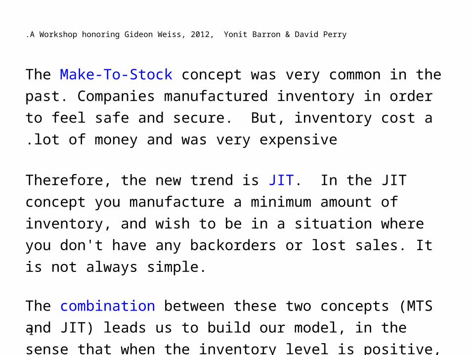
The Make-To-Stock concept was very common in the past. Companies

manufactured inventory in order to feel safe and secure. But, inventory

cost a lot of money and was very expensive.

Therefore, the new trend is JIT. In the JIT concept you manufacture a

minimum amount of inventory, and wish to be in a situation where you

don't have any backorders or lost sales. It is not always simple.

The combination between these two concepts (MTS and JIT) leads us to

build our model, in the sense that when the inventory level is positive, the

production rate is low and when the inventory level is negative, the

production rate is high.

2

A Workshop honoring Gideon Weiss, 2012, Yonit Barron & David Perry.

A Jump Fluid Production-

Inventory Model with a Double

Band Control

Yonit Barron, David Perry.

Haifa University

Israel

3

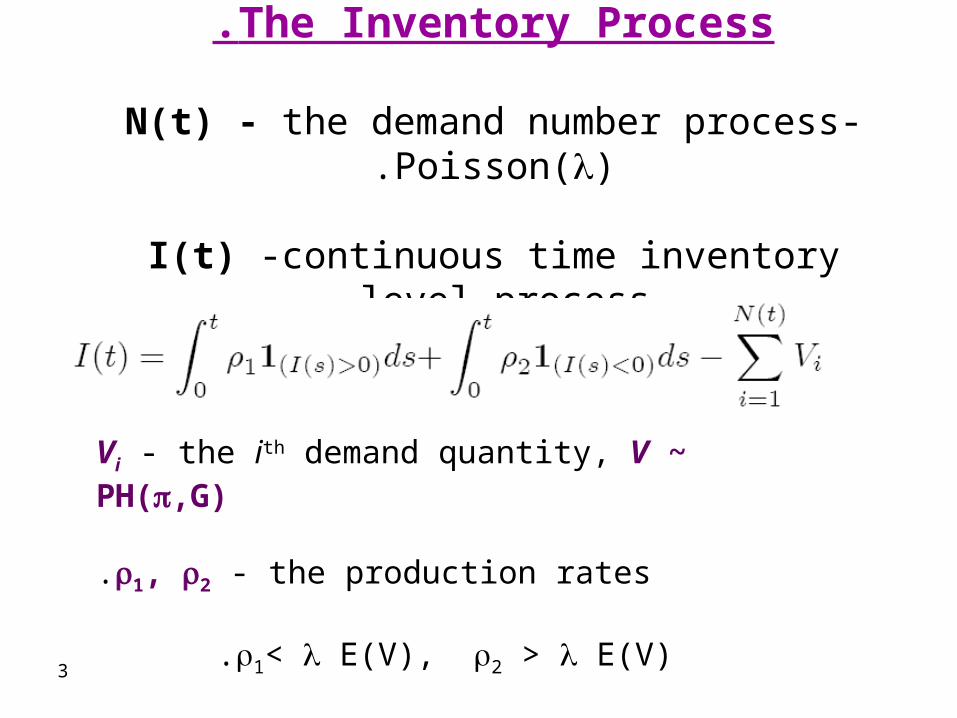
The Inventory Process.

N(t) - the demand number process- Poisson().

I(t) -continuous time inventory level process.

Vi - the ith demand quantity, V ~ PH(,G)

1, 2 - the production rates.

1< E(V), 2 > E(V).

4

The storage capacity is finite with level b.

Backordering to a level (-a) is allowed. Any backlog that

exceeds level (-a) is lost.

1 2

T1 T2

Ĭ(t)

t

b

0

-a

Ĭ+(t) - positive process

Ĭ-(t) - negative process

holding cost

idle cost

shortage costlost sale cost

5

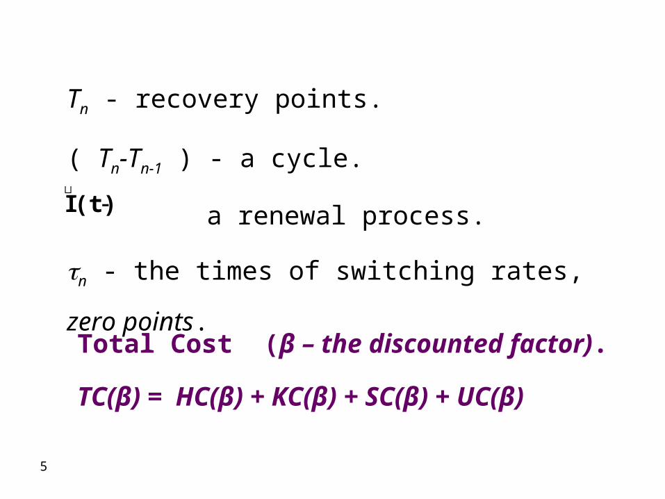
Tn - recovery points.

( Tn-Tn-1 ) - a cycle.

a renewal process.

n - the times of switching rates, zero points.

Total Cost (β – the discounted factor).

TC(β) = HC(β) + KC(β) + SC(β) + UC(β)

(t)I

6

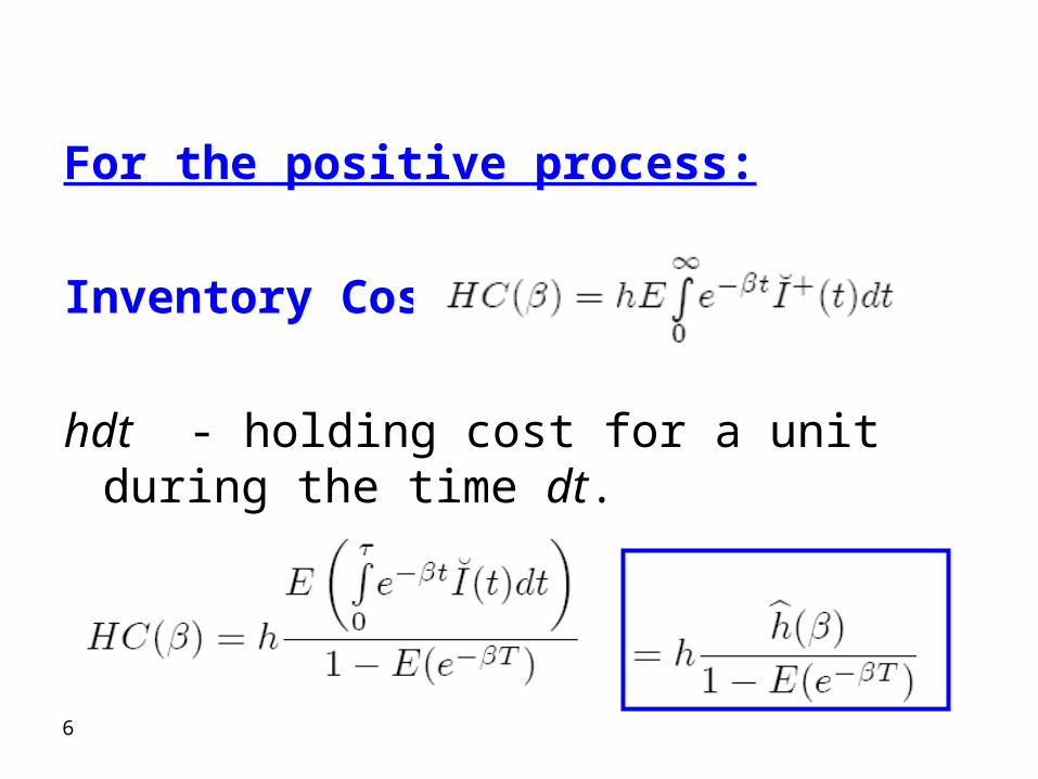
For the positive process:

Inventory Cost.

hdt - holding cost for a unit during the time dt.

7

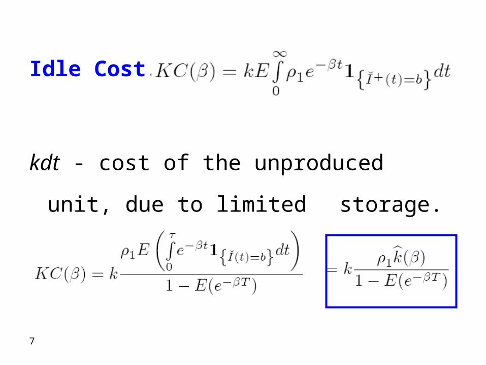
Idle Cost.

kdt - cost of the unproduced unit, due to limited

storage.

8

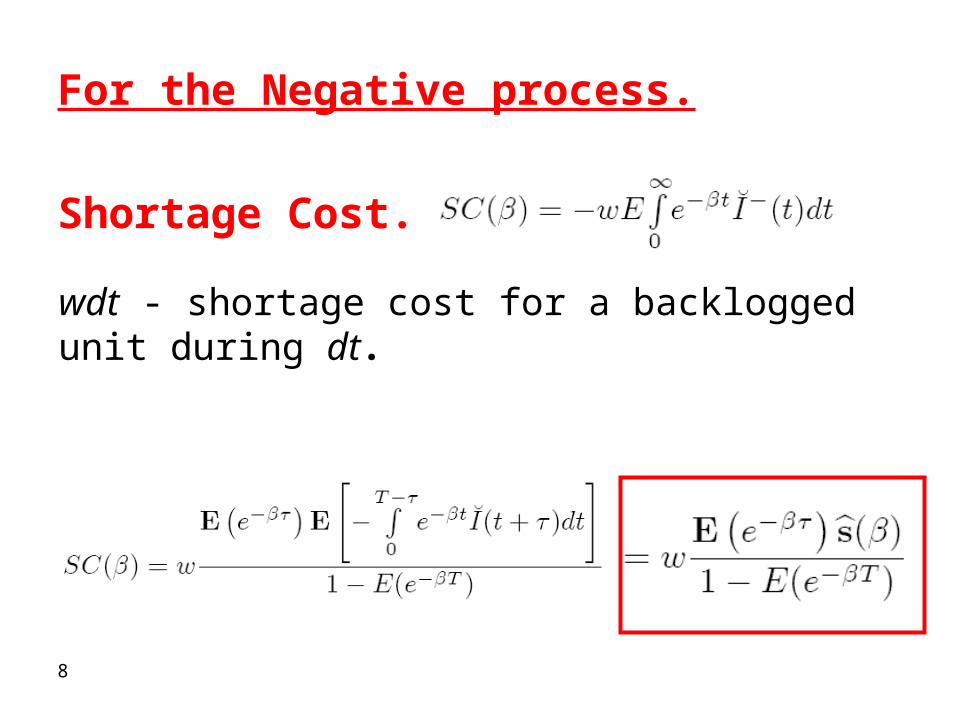
For the Negative process.

Shortage Cost.

wdt - shortage cost for a backlogged unit during dt.

9

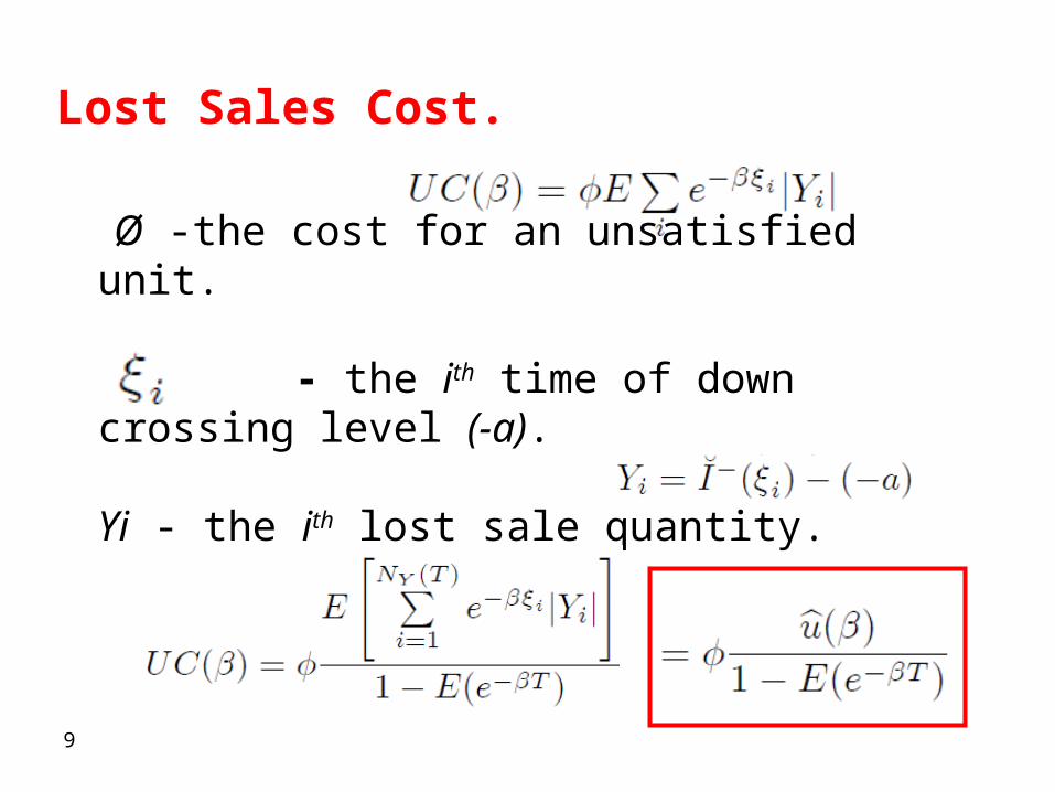
Lost Sales Cost.

Ø -the cost for an unsatisfied unit.

- the ith time of down crossing level (-a).

Yi - the ith lost sale quantity.

10

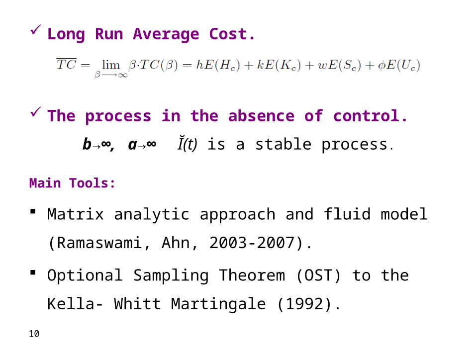
Long Run Average Cost.

The process in the absence of control.

b→∞, a→∞ Ĭ(t) is a stable process.

Main Tools:

Matrix analytic approach and fluid model (Ramaswami, Ahn,

2003-2007).

Optional Sampling Theorem (OST) to the Kella- Whitt

Martingale (1992).

11

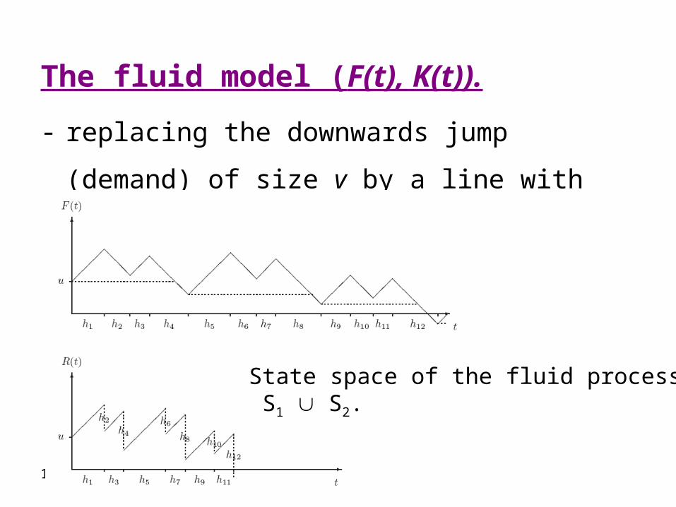
The fluid model (F(t), K(t)).

- replacing the downwards jump (demand) of size v by

a line with slope (-).

State space of the fluid process – S1 S2.

12

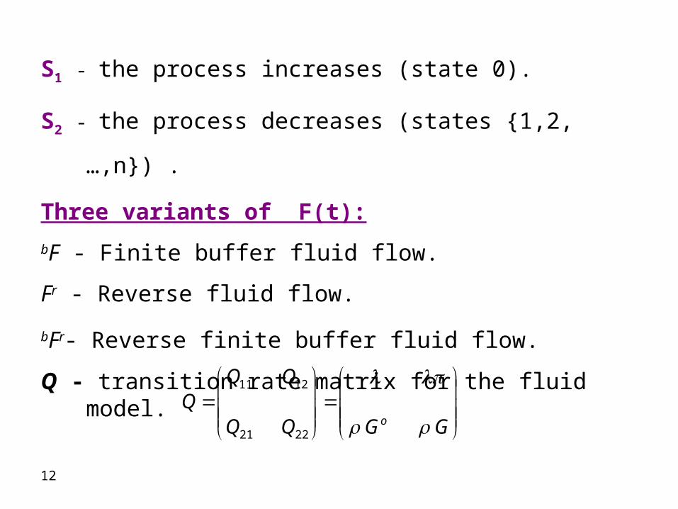
S1 - the process increases (state 0).

S2 - the process decreases (states {1,2,…,n}) .

Three variants of F(t):

bF - Finite buffer fluid flow.

Fr - Reverse fluid flow.

bFr- Reverse finite buffer fluid flow.

Q - transition rate matrix for the fluid model.

GGQQ

QQQ

o 2221

1211

13

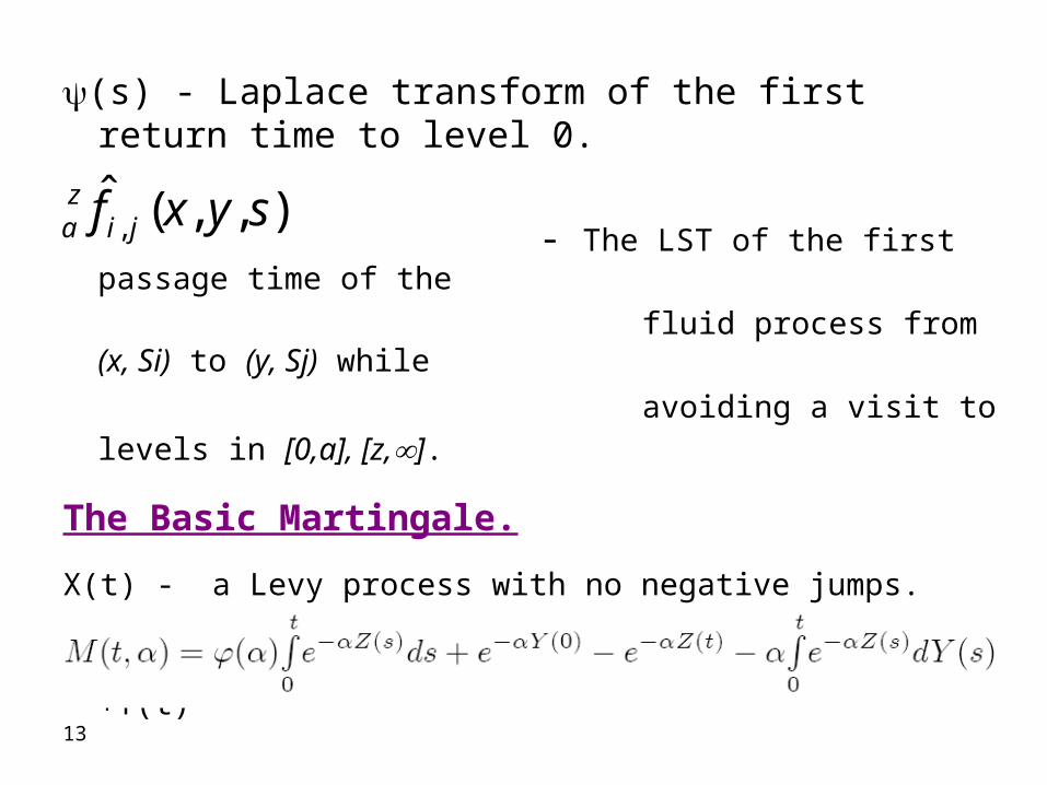
(s) - Laplace transform of the first return time to level 0.

- The LST of the first passage time of the

fluid process from (x, Si) to (y, Sj) while

avoiding a visit to levels in [0,a], [z,].

The Basic Martingale.

X(t) - a Levy process with no negative jumps.

Y(t) - an adapted process Z(t)=X(t)+Y(t)

),,(ˆ, syxf ji

za

14

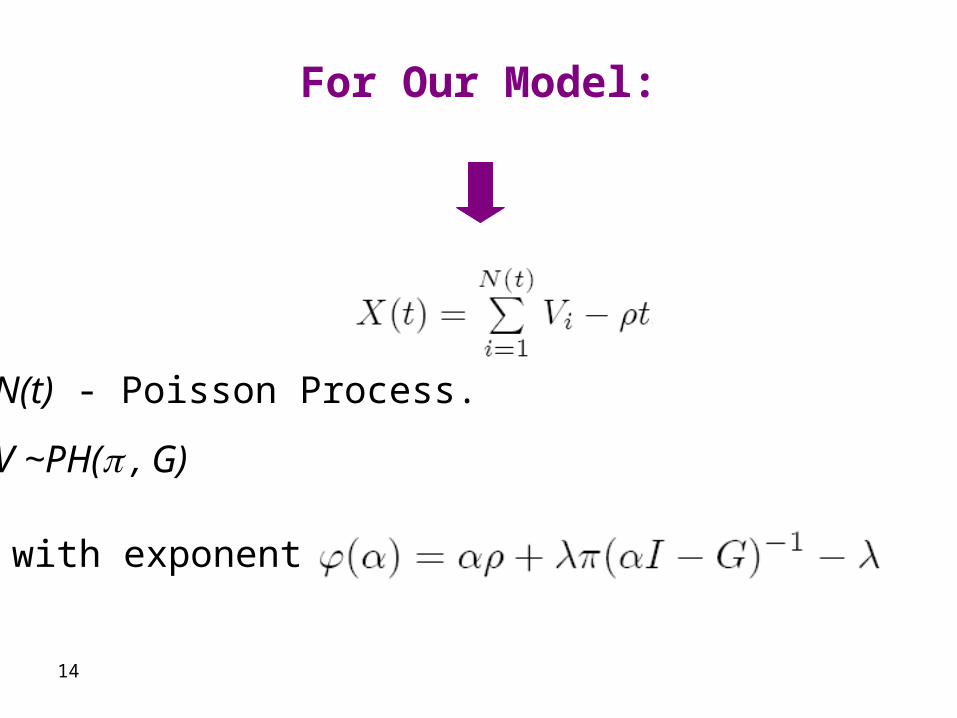
For Our Model:

N(t) - Poisson Process.

V ~PH( , G)

with exponent

15

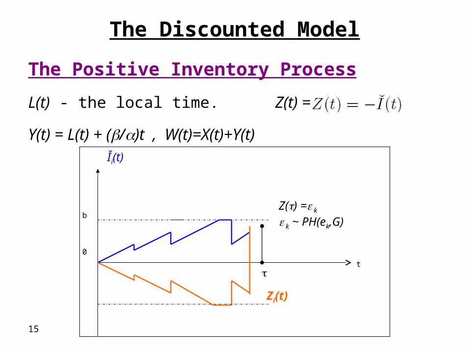
The Discounted Model

The Positive Inventory Process

L(t) - the local time. Z(t) = X(t) + L(t) →

Y(t) = L(t) + (/)t , W(t)=X(t)+Y(t)Ĭi(t)

t

b

0

Zi(t)

Z() = k

k ~ PH(ek,G)

16

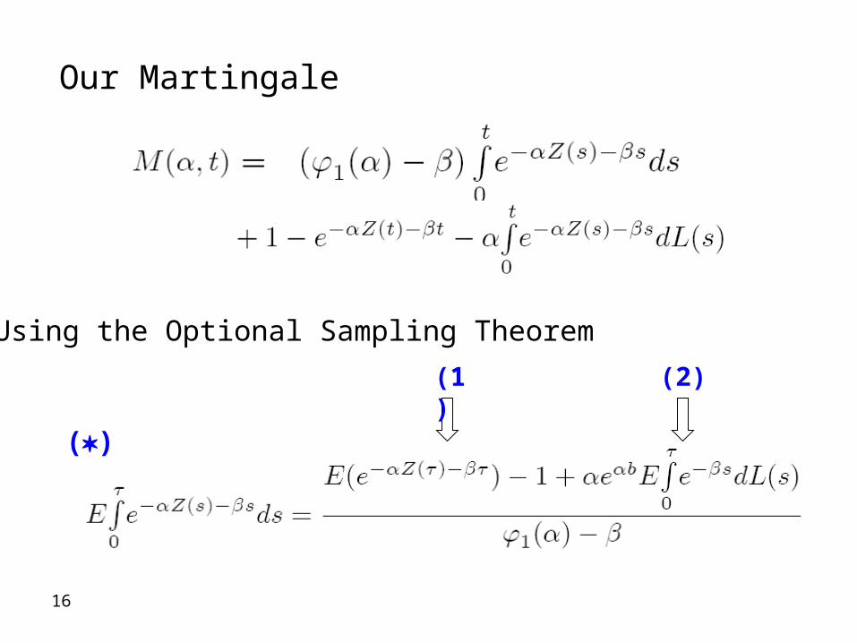
Our Martingale

Using the Optional Sampling Theorem:

(2)(1)

()

17

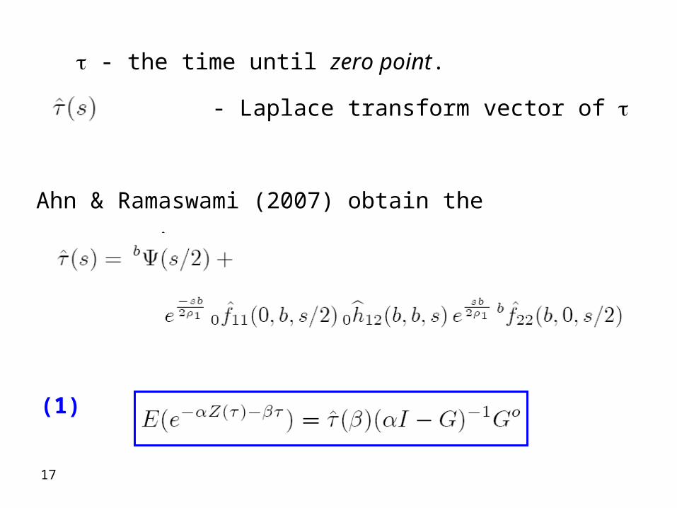
- the time until zero point.

- Laplace transform vector of

Ahn & Ramaswami (2007) obtain the expression:

(1)

18

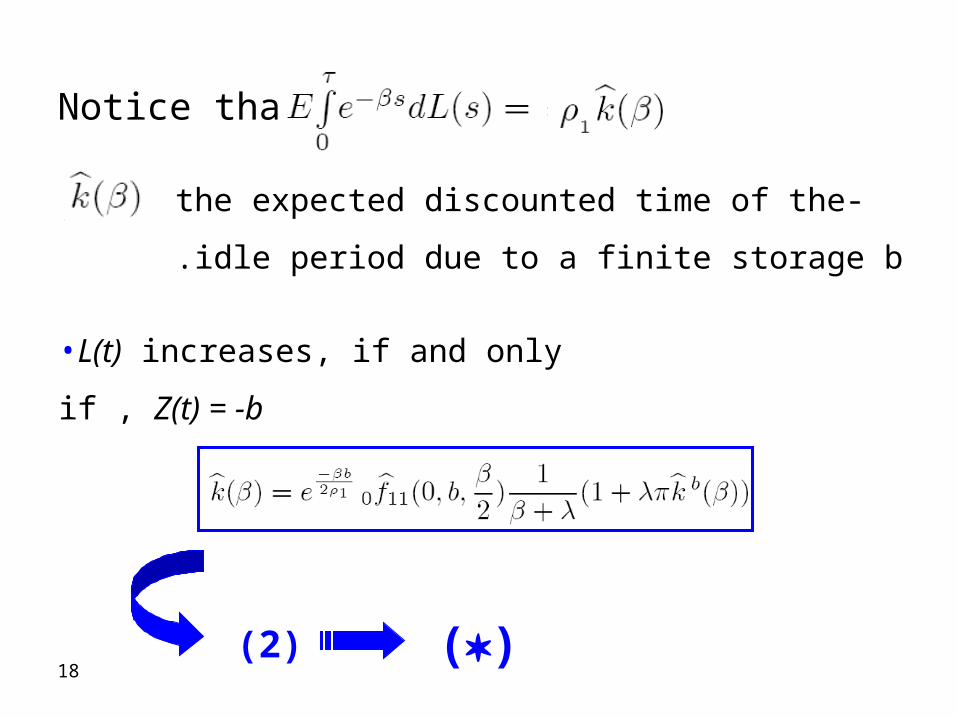
Notice that:

-the expected discounted time of the idle period due to a

finite storage b.

)2( )(

•L(t) increases, if and only if , Z(t) = -b

19

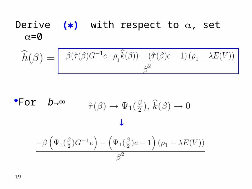
Derive () with respect to , set =0

For b→∞

20

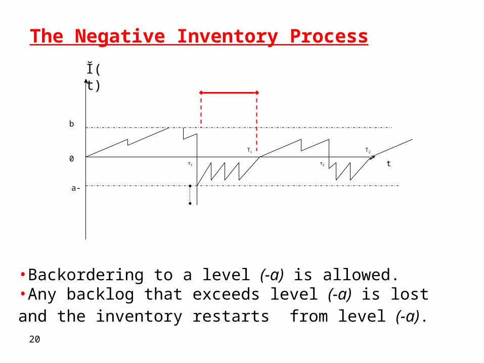
The Negative Inventory Process

1 2

T1 T2

Ĭ(t)

t

b

0

-a

•Backordering to a level (-a) is allowed.•Any backlog that exceeds level (-a) is lost and the inventory restarts from level (-a).

21

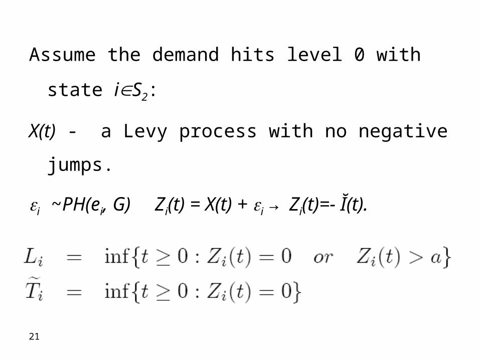
Assume the demand hits level 0 with state iS2:

X(t) - a Levy process with no negative jumps.

i ~PH(ei, G) Zi(t) = X(t) + i → Zi(t)=- Ĭ(t).

Two stopping times:

22

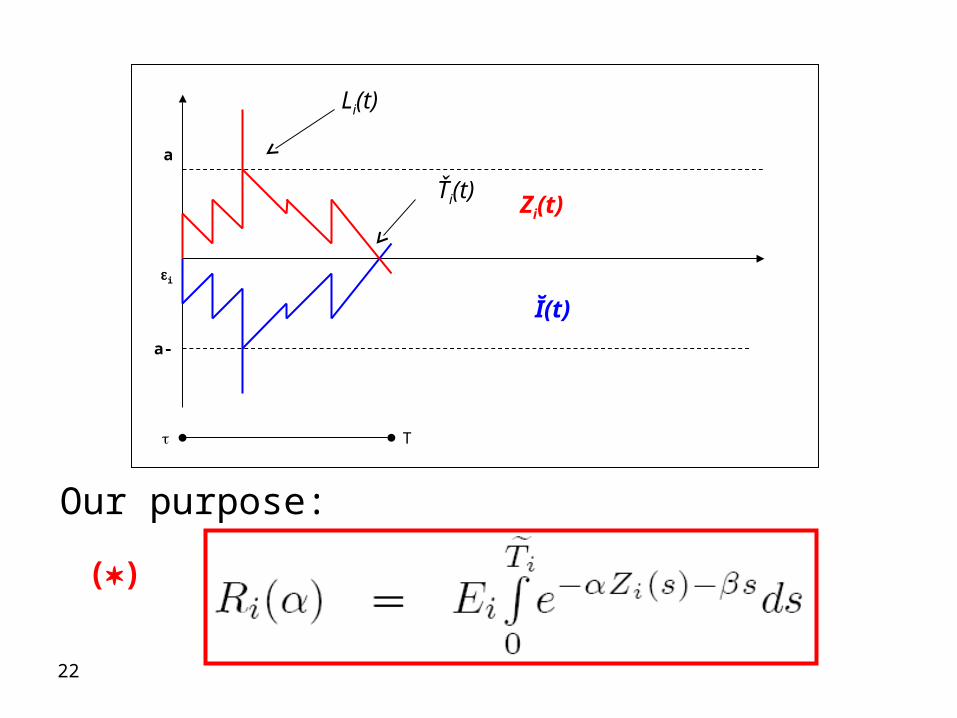
Our purpose:

()

T

-a

a

Ĭ(t)

Zi(t)

i

Li(t)

Ťi(t)

23

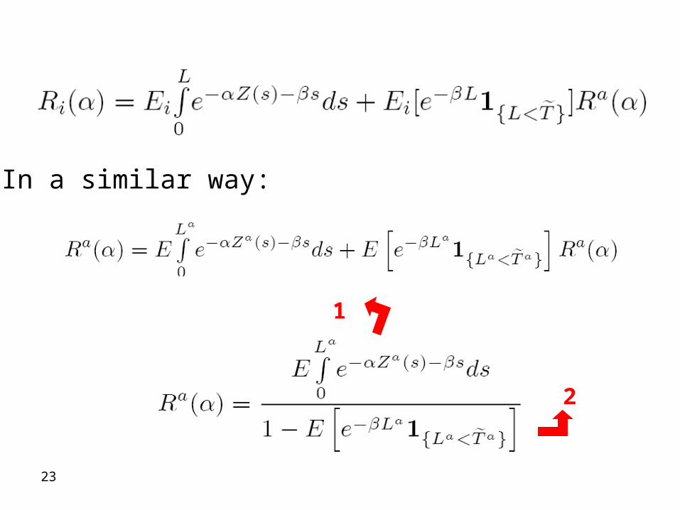
In a similar way:

1

2

24

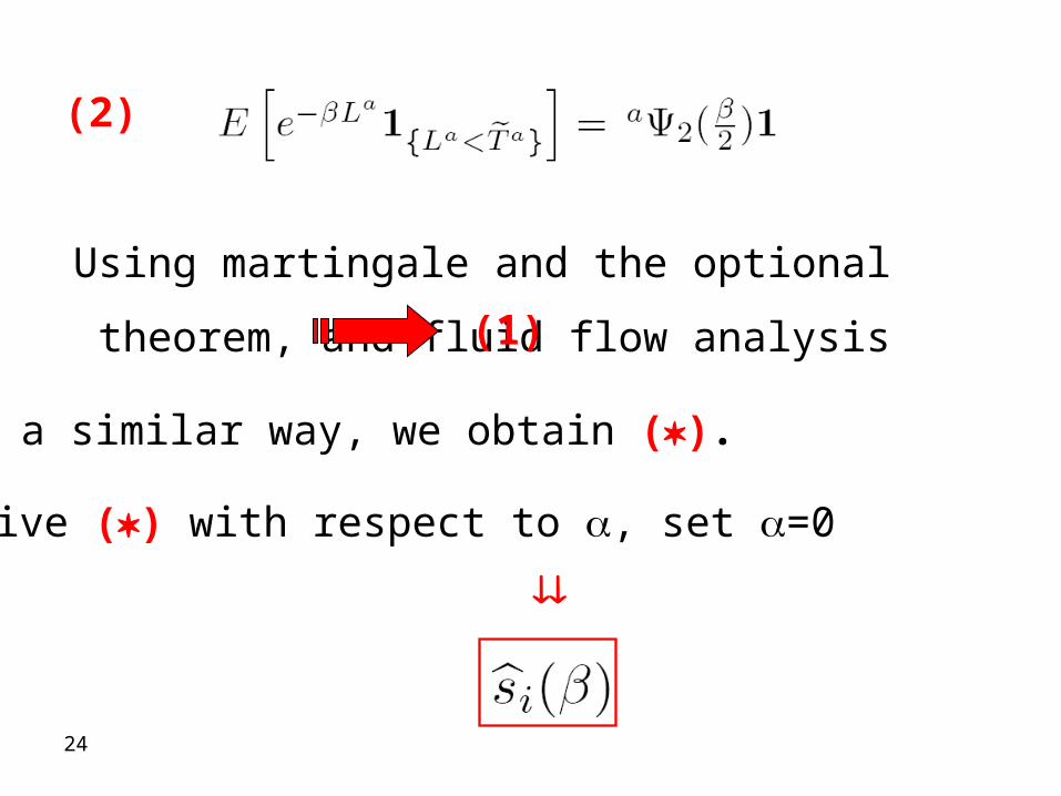
(2)

Using martingale and the optional theorem, and fluid

flow analysis )1(

In a similar way, we obtain ().

Derive () with respect to , set =0

25

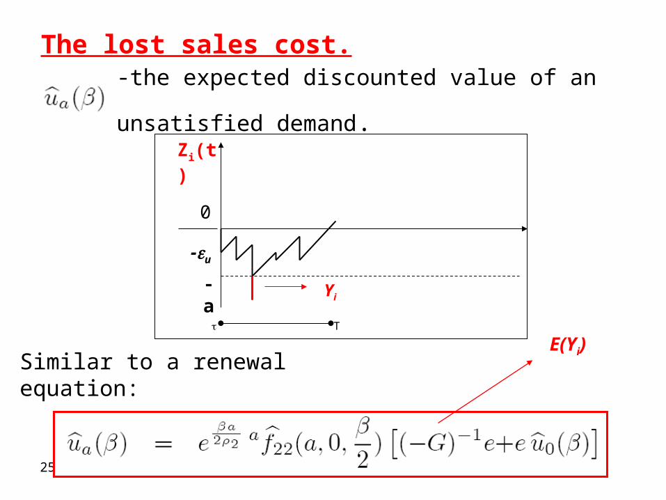
The lost sales cost.

-the expected discounted value of an unsatisfied demand.

Similar to a renewal equation:

T

-a

Zi(t)

-u

0

Yi

E(Yi)

26

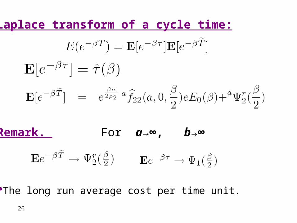
Remark. For a→∞, b→∞

The long run average cost per time unit.

Laplace transform of a cycle time:

27

A Workshop honoring Gideon Weiss, 2012, Yonit Barron & David Perry.