A welfare perspective on the fiscal–monetary policy mix: The role of alternative fiscal...
33
Journal of Policy Modeling 33 (2011) 920–952 Available online at www.sciencedirect.com A welfare perspective on the fiscal–monetary policy mix: The role of alternative fiscal instruments Luigi Marattin a,∗ , Massimiliano Marzo b , Paolo Zagaglia c a Department of Economics, Universitá di Bologna b Department of Economics, Universitá di Bologna c Modelling Unit, Sveriges Riksbank Received 1 October 2010; received in revised form 1 November 2010; accepted 1 February 2011 Available online 2 April 2011 Abstract The need of fiscal consolidation is likely to dominate the policy agenda in the next decade; starting from statistical evidence on the conduct of fiscal policy in the EMU area over the last decade, this paper addresses the optimality of alternative fiscal consolidation strategies. In this paper, we explore the welfare properties of debt-targeting fiscal policy implemented through, alternatively, distortionary taxation on consumption, labour and capital income or productive and wasteful government expenditure. We build a general equilibrium model with various distortions in order to evaluate the welfare ranking of alternative fiscal policy configurations under different monetary policy regimes. Our results show the welfare superiority of fiscal adjustments based on productive government expenditure, whereas the use of a capital income tax rate as fiscal instruments yields the highest welfare loss. © 2011 Society for Policy Modeling. Published by Elsevier Inc. All rights reserved. JEL classification: E62; E63 Keywords: Welfare analysis; Optimal policy rules; Fiscal and monetary policy; Inflation stabilization The views expressed herein are those of the authors only and should not be attributed to the members of the Executive Board of Sveriges Riksbank. ∗ Corresponding author. Tel.: +39 051 2092606. E-mail addresses: [email protected] (L. Marattin), [email protected] (M. Marzo), [email protected] (P. Zagaglia). 0161-8938/$ – see front matter © 2011 Society for Policy Modeling. Published by Elsevier Inc. All rights reserved. doi:10.1016/j.jpolmod.2011.03.003
-
Upload
luigi-marattin -
Category
Documents
-
view
213 -
download
0
Transcript of A welfare perspective on the fiscal–monetary policy mix: The role of alternative fiscal...

Journal of Policy Modeling 33 (2011) 920–952
Available online at www.sciencedirect.com
A welfare perspective on the fiscal–monetary policymix: The role of alternative fiscal instruments�
Luigi Marattin a,∗, Massimiliano Marzo b, Paolo Zagaglia c
a Department of Economics, Universitá di Bolognab Department of Economics, Universitá di Bologna
c Modelling Unit, Sveriges Riksbank
Received 1 October 2010; received in revised form 1 November 2010; accepted 1 February 2011Available online 2 April 2011
Abstract
The need of fiscal consolidation is likely to dominate the policy agenda in the next decade; starting fromstatistical evidence on the conduct of fiscal policy in the EMU area over the last decade, this paper addressesthe optimality of alternative fiscal consolidation strategies. In this paper, we explore the welfare properties ofdebt-targeting fiscal policy implemented through, alternatively, distortionary taxation on consumption, labourand capital income or productive and wasteful government expenditure. We build a general equilibrium modelwith various distortions in order to evaluate the welfare ranking of alternative fiscal policy configurationsunder different monetary policy regimes. Our results show the welfare superiority of fiscal adjustments basedon productive government expenditure, whereas the use of a capital income tax rate as fiscal instrumentsyields the highest welfare loss.© 2011 Society for Policy Modeling. Published by Elsevier Inc. All rights reserved.
JEL classification: E62; E63
Keywords: Welfare analysis; Optimal policy rules; Fiscal and monetary policy; Inflation stabilization
� The views expressed herein are those of the authors only and should not be attributed to the members of the ExecutiveBoard of Sveriges Riksbank.
∗ Corresponding author. Tel.: +39 051 2092606.E-mail addresses: [email protected] (L. Marattin), [email protected] (M. Marzo),
[email protected] (P. Zagaglia).
0161-8938/$ – see front matter © 2011 Society for Policy Modeling. Published by Elsevier Inc. All rights reserved.doi:10.1016/j.jpolmod.2011.03.003

L. Marattin et al. / Journal of Policy Modeling 33 (2011) 920–952 921
1. Introduction
The process of cutting-back the massive stock of public debt accumulated after the 2008-2009recession is likely to dominate the policy debate over the next decade. Table 1 shows the changein levels of the debt/GDP ratio in major industrialized countries from 2007 to 2010.
These figures suggest that the question is not so much whether to implement a fiscal consolida-tion, but rather how to do it. Specifically, whether it would be preferable to carry it out by cuttingpublic expenditure or by increasing average tax rates on factor incomes and consumption.
The issue of whether fiscal adjustments should rely on the expenditure rather than the revenueside is hardly a new topic in the policy debate. Its importance was already emphasized by theJanuary 2004 ECB Monthly Bulletin (p.46)
“The composition of the budgetary adjustment is particularly relevant, there being evidencethat an expenditure-based adjustment tends to be more growth-friendly and long-lived thana tax-based adjustment without expenditure retrenchment.”
Looking at the case-studies of Ireland and Denmark in the Eighties, Giavazzi and Pagano (1990)were the first ones to suggest that fiscal adjustments implemented on the government spendingside could be expansionary. This view is confirmed by Alesina and Perotti (1997), who examine afull sample of OECD countries and find that adjustments relying on government expenditure cutshad a better chance of being successful and expansionary; on the other hand, if they are based ontax increases and cuts in public investments, tend not to be non-persistent and contractionary. Thisresult is strengthened by Alesina and Ardagna (2009) who extend the analysis up to 2007. Usinga panel OECD from 1970 to 2007, they define fiscal adjustments (stimuli) as episodes wherethe cyclically adjusted primary balance improves (deteriorates) by at least 1.5 per cent of GDP.Subsequently they investigate whether such episodes – that differ in size and composition – areassociated with booms or recessions and with success in debt stabilization. Their conclusion is thatmost successful fiscal adjustments are those in which a larger share of the reduction of primarydeficit is due to cuts in current spending (wage and non-wage component) and to subsidies.
Based on these considerations, in this paper we introduce a new dimension to assess thedesiderability of alternative debt-stabilizing plans: what are the welfare effects (and not simply
Table 1Evolution of Debt/GDP ratio, major industrialized countries.
Country Debt/GDP 2007 Debt/GDP 2010
Ireland 24.80 79.70Luxembourg 7 14.50Spain 36.20 62.30United Kingdom 44.15 71United States 63.05% 91.57Netherlands 45.70 63.10Finland 35.10 45.70Portugal 63.60 81.50Denmark 26.84 33.66Germany 65.10 78.70Belgium 83.90 100.90Japan 167.10 193.97Italy 104.10 116.10

922 L. Marattin et al. / Journal of Policy Modeling 33 (2011) 920–952
the growth effects) of fiscal adjustments based on the expenditure rather than on the revenue side?To accomplish this task, we adopt a suitable DSGE framework calibrated on the Euro area, as thefocus of our analysis is mainly targeted at the EU policy debate. As we employ a workhorse forpolicy analysis, as the DSGE model has become, we also refer to the related rich literature on theinteractions between monetary and fiscal policy.
The seminal contribution by Leeper (1991), featured by Ricardian environment and lump-sumtaxation, established the parameter conditions for local equilibrium determinacy based essentiallyon the size of monetary policy’s response to inflation. If Taylor’s principle holds, determinacy ispreserved regardless on fiscal policy’s active or passive stance. This implies that monetary policyis conducted without any influence arising from fiscal considerations: the fiscal authority merelyraises tax revenue so to balance the intertemporal budget constraint, and the dynamic of debtis the main factor determining the tax stance1. If, alternatively, monetary policy’s feedback ruleis not enough to affect the real interest rate,an active role of fiscal policy is needed to restoreequilibrium determinacy. In particular, another strand of literature (“the fiscal theory of the pricelevel”, Woodford (1994); Sims (1994), (Canzoneri, Cumby, & Diba, 2001)) stresses the likelyemergence of price level adjustments that are automatically needed in order to guarantee theintertemporal solvency of government budget constraint.
Ever since Leeper (1991) the literature began to relax some of the simplifying assumptionswhich were part of the original framework, in order to be able to study the interactions betweenfiscal and monetary policy in a richer and more realistic framework2.Basically, contributions differinsofar as they employ alternatives strategies to depart from Ricardian equivalence. One strand ofliterature models the presence of non-Ricardian consumers à-la Blanchard (1985), by assuming anon-zero probability of death for households (Leith and Wren-Lewis, 2000; Chadha and Nolan,2007). Under this specification, consumers’finite-horizon implies a wealth effect of governmentdebt on aggregate consumption via the Euler equation. In this scenario Leith and Thadden (2008)prove not only that steady-state government debt becomes a crucial state variable for determinacyof local equilibrium and its dynamics, but also that its level is important: the required degree offiscal discipline is an increasing (but yet discontinuos) function of the debt level when monetarypolicy is to become more active3. Other contributions have broken Ricardian equivalence byintroducing distortionary taxation, and have looked at the non-trivial interactions with monetarypolicy (Schmitt-Grohé and Uribe, 2004c, 2007; Edge and Rudd, 2002; Linnemann, 2006).
Our paper follows this latter approach, insofar as we introduce (multiple) distortionary taxationand implement a welfare analysis via second-order perturbation methods. Furthermore, the noveltyof our contribution lies in the emphasis on the choice of the fiscal instrument. Particularly, we builda dynamic stochastic general equilibrium (DSGE) model with multiple sources of distortions, andperform a welfare evaluation of the use of different fiscal instruments. In particular, we compare
1 In many contributions that have borrowed and modified the original Leeper’s framework (Sims, 1994; Davig andLeeper, 2005; Schmitt-Grohé and Uribe, 2004a; Leith and Thadden, 2008), the relevant parameter of the fiscal rule isthe feedback coefficient of (lump-sum) taxes on debt. The fiscal stance is passive if the coefficient is larger than thesteady-state real interest rate, active otherwise. Leith and Thadden (2008) note that many authors typically tighten thedefinition of fiscal policy to one ensuring not only the solvency of intertemporal budget constraint, but also stationarityof government debt.
2 While acknowledging many significant open-economy contributions (Linnemann, 2006; Leith and Wren-Lewis, 2000),we focus here on closed-economy investigations.
3 Their paper also links the approach à-la-Blanchard with an alternative way to introduce non-Ricardian consumers,namely the use of credit-constrained (or “rule-of-thumb”) agents (Galì, Lopez-Salido, and Vallès (2004), Bilbie (2009)).They show that the crucial qualitative results are robust to the alternative specifications.

L. Marattin et al. / Journal of Policy Modeling 33 (2011) 920–952 923
the welfare properties of rules for fiscal policy that prescribe changes in different tax rates or typesof government spending. Within each of these two categories, we operate a further distinction:on the spending side between government consumption and productive public spending, whereason the revenue side between three types of distortionary taxation (on consumption, labour andcapital income). Our analysis also distinguishes between monetary policy based on interest rateor money growth rules.
The perspective we adopt is rather widespread in policy analysis. The role played byfiscal and monetary policy mix has been analyzed by Lossani, Natale, and Tirelli (2003),who explore how alternative monetary arrangements perform when the fiscal authority pur-sues a long-term debt reduction strategy, but yet retain fiscal flexibility to counteract supplyshocks. In an open-economy setting, Tirelli (1992) evaluates coordination in the form of sim-ple rules, finding support for monetary policy to be concerned with inflation control andfiscal policy to be assigned a foreign wealth target. In line with our focus on the EU area,Annichiarico (2007) investigates the inflationary effects of fiscal policy in a DSGE model cal-ibrated with quarterly EU data, finding that government deficits, high debt levels and slowfiscal adjustments adversely affect price stability when monetary policy adopt a monetary targetregime.
We obtain a number of results. We find that fiscal consolidation based on productive governmentexpenditure (defined broadly as public spending enhancing the marginal product of capital andlabour in the production function) is welfare-superior to other specifications. On the other hand, fis-cal adjustment based on capital-income taxation generally bring about the highest welfare losses.These ‘corners’ of targeting instruments’welfare ranking seem robust to a various specifications ofthe interest-rate rule, and even to an alternative specifications of monetary policy based on moneygrowth. These results are not significantly reversed even if we assign a ‘useful’ role to governmentconsumption, by inserting it additively into the utility function (e.g., see Linnemann and Schabert,2004). Another relevant result concerns the ranking of (unconditional) welfare losses according tothe degree of distortions in the economy. For any given fiscal instrument, the departure from per-fect competition and the presence of money yields greater welfare losses than the introduction ofprice rigidity within a monopolistic competition framework. We believe our result concerning thewelfare-superiority of a government spending rule as fiscal instrument to be particularly relevantfor daily policy-making. Recent experiences (primary UK, but also Italy although to a lesser extent)attempted to peg government spending dynamics to the evolution of macroeconomic targets.Our framework can contribute to a better understanding of the relative desiderability of such anoption.
This paper is organized as follows. Section 2 presents some statistical evidence which isuseful to pave the way for the normative analysis. Section 3 describes the theoretical model.Section 4 outlines the computational strategy for the solution of the model. Section 5 discussesthe calibration of the model. Section 6 outlines the quantitative results. Section 7 presents someconcluding remarks.
2. Empirical Evidence
Our theoretical question regards the welfare properties of fiscal consolidation, defined as anegative reaction of budget deficit to public debt accumulation. In this section we present ourown econometric evidence regarding the plausibility of such an investigation using Euro-areaaggregate quarterly data from 1999 to 2010. Particularly, in subsection 2.1. we estimate a Struc-tural Vector AutoRegressive model in order to obtain an empirical characterization of primary

924 L. Marattin et al. / Journal of Policy Modeling 33 (2011) 920–952
deficit’s movements in response to debt. In subsection 2.2. we perform a correlation analysisfocused on the relationship between budget deficit’s components and the stock of governmentliabilities.
2.1. A SVAR Analysis on the EU area
In this subsection we build and estimate a VAR model to illustrate the dynamics of averageEU fiscal positions after a public debt shock.
The general structural form of model is given by:
A0Xt = A(L)Xt−1 + ut (1)
where Xtis a m x 1 vector of endogenous variables, A0 is a m x m matrix capturing contempora-neous relations among variables; A(L) is a finite-order vector polynomial in non-negative powersof the lag operator; finally ut is the m x 1 structural disturbance vector. Pre-multypling (1) by A−1
0we obtain the reduced form we can actually estimate:
Xt = B(L)Xt−1 + ξt (2)
where B(L) = A(L)A−10 and ξt = A−1
0 ut is the reduced-form residual vector.Our first attempt consider m = 3, so that vector Xt is given by:
Xt = [Yt, DPRt , Bt]
where Yt is real GDP, DPRt is primary deficit, Bt is real stock of government debt. All variablesare seasonally-adjusted. We use quarterly EU data taken from Thomson Datastream. The sampleperiod is 1999Q1-2010:Q1.
Identification is achieved through a standard lower-triangular Cholesky scheme, where weallow within-the-quarter effect of real activity on everything else and of primary deficit on debt.
Fig. 2 shows the response of real output and deficit to a one-standard-deviation shock ingovernment debt.
The left-hand panel shows a negative reaction of economic activity to debt-shocks, although thestatistical significance ceases after 3 quarters. More interestingly, the right-hand-panel indicatesthat EU-aggregate primary deficit reduces after increase in the stock of government liabilities.This suggests the presence of a debt-stabilizing motive in the conduct of EU fiscal policy in thelast ten years.
We test the robustness of our central result by extending to m = 4 the dimension of vector X,which is now made by:
Xt = [Yt, DPRt , Bt, πt]
where πt is the CPI inflation index4. In this case we added the inflation rate which is allowed tobe affected within the quarter by all other macroeconomic variables. Fig. 3 displays the impulseresponse functions relative to this new specification.The picture confirms the negative responseof primary deficit after an increase in the stock of government debt.
Our SVAR estimation seems pretty robust in indicating a debt-stabilizing motive in the conductof fiscal policy during Euro’s first decade. Before turning to a formal model to investigate the
4 Note that we cannot further extend the dimension of our VAR, given the relatively limited number of observations.This constraint, in turn, is given by our focus on the EU aggregate area.
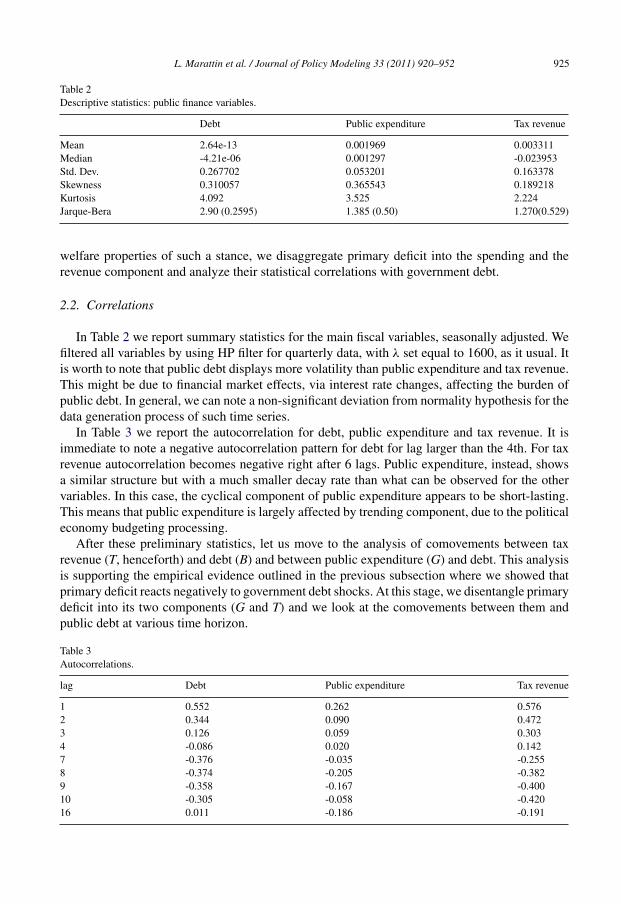
L. Marattin et al. / Journal of Policy Modeling 33 (2011) 920–952 925
Table 2Descriptive statistics: public finance variables.
Debt Public expenditure Tax revenue
Mean 2.64e-13 0.001969 0.003311Median -4.21e-06 0.001297 -0.023953Std. Dev. 0.267702 0.053201 0.163378Skewness 0.310057 0.365543 0.189218Kurtosis 4.092 3.525 2.224Jarque-Bera 2.90 (0.2595) 1.385 (0.50) 1.270(0.529)
welfare properties of such a stance, we disaggregate primary deficit into the spending and therevenue component and analyze their statistical correlations with government debt.
2.2. Correlations
In Table 2 we report summary statistics for the main fiscal variables, seasonally adjusted. Wefiltered all variables by using HP filter for quarterly data, with λ set equal to 1600, as it usual. Itis worth to note that public debt displays more volatility than public expenditure and tax revenue.This might be due to financial market effects, via interest rate changes, affecting the burden ofpublic debt. In general, we can note a non-significant deviation from normality hypothesis for thedata generation process of such time series.
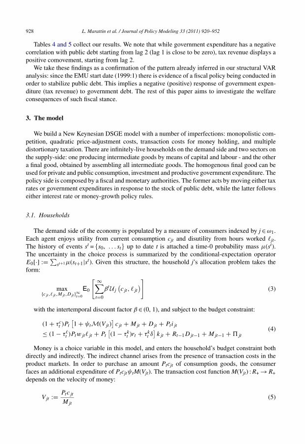
In Table 3 we report the autocorrelation for debt, public expenditure and tax revenue. It isimmediate to note a negative autocorrelation pattern for debt for lag larger than the 4th. For taxrevenue autocorrelation becomes negative right after 6 lags. Public expenditure, instead, showsa similar structure but with a much smaller decay rate than what can be observed for the othervariables. In this case, the cyclical component of public expenditure appears to be short-lasting.This means that public expenditure is largely affected by trending component, due to the politicaleconomy budgeting processing.
After these preliminary statistics, let us move to the analysis of comovements between taxrevenue (T, henceforth) and debt (B) and between public expenditure (G) and debt. This analysisis supporting the empirical evidence outlined in the previous subsection where we showed thatprimary deficit reacts negatively to government debt shocks. At this stage, we disentangle primarydeficit into its two components (G and T) and we look at the comovements between them andpublic debt at various time horizon.
Table 3Autocorrelations.
lag Debt Public expenditure Tax revenue
1 0.552 0.262 0.5762 0.344 0.090 0.4723 0.126 0.059 0.3034 -0.086 0.020 0.1427 -0.376 -0.035 -0.2558 -0.374 -0.205 -0.3829 -0.358 -0.167 -0.40010 -0.305 -0.058 -0.42016 0.011 -0.186 -0.191

926
L.
Marattin
et al.
/ Journal
of Policy
Modeling
33 (2011)
920–952
Table 4Comovements between tax revenues and debt.
T( − 4) T( − 3) T( − 2) T( − 1) T B B( − 1) B( − 2) B( − 3) B( − 4)
T( − 4) 1 0.830879 0.715823 0.503064 0.289233 -0.664811 -0.759110 -0.765771 -0.573944 -0.340766T( − 3) 0.830879 1 0.844746 0.727933 0.525964 -0.802929 -0.816113 -0.652965 -0.381549 -0.055828T( − 2) 0.715823 0.844746 1 0.850017 0.738008 -0.844895 -0.712474 -0.471000 -0.100757 0.214558T( − 1) 0.503064 0.727933 0.850017 1 0.856572 -0.732298 -0.527237 -0.187339 0.176171 0.430750T 0.289233 0.525964 0.738008 0.856572 1 -0.549514 -0.256638 0.095749 0.412224 0.584877B -0.664811 -0.802929 -0.844895 -0.732298 -0.549514 1 0.889284 0.621397 0.223835 -0.132405B( − 1) -0.759110 -0.816113 -0.712474 -0.527237 -0.256638 0.889284 1 0.858610 0.559922 0.229826B( − 2) -0.765771 -0.652965 -0.471000 -0.187339 0.095749 0.621397 0.858610 1 0.846386 0.616357B( − 3) -0.573944 -0.381549 -0.100757 0.176171 0.412224 0.223835 0.559922 0.846386 1 0.882457B( − 4) -0.340766 -0.055828 0.214558 0.430750 0.584877 -0.132405 0.229826 0.616357 0.882457 1

L.
Marattin
et al.
/ Journal
of Policy
Modeling
33 (2011)
920–952
927
Table 5Comovements between public expenditure and debt.
G( − 4) G( − 3) G( − 2) G( − 1) G B B( − 1) B( − 2) B( − 3) B( − 4)
G( − 4) 1 0.364925 0.062835 -0.019242 0.054144 0.118806 0.157683 0.195530 0.198999 0.091626G( − 3) 0.364925 1 0.387646 0.105342 0.101653 0.356101 0.401539 0.340942 0.115539 -0.145015G( − 2) 0.062835 0.387646 1 0.395651 0.134373 0.422112 0.368110 0.156932 -0.142759 -0.270028G( − 1) -0.019242 0.105342 0.395651 1 0.403634 0.369069 0.179650 -0.110658 -0.281824 -0.439992G 0.054144 0.101653 0.134373 0.403634 1 0.254686 0.007393 -0.196334 -0.441538 -0.508754B 0.118806 0.356101 0.422112 0.369069 0.254686 1 0.889284 0.621397 0.223835 -0.132405B( − 1) 0.157683 0.401539 0.368110 0.179650 0.007393 0.889284 1 0.858610 0.559922 0.229826B( − 2) 0.195530 0.340942 0.156932 -0.110658 -0.196334 0.621397 0.858610 1 0.846386 0.616357B( − 3) 0.198999 0.115539 -0.142759 -0.281824 -0.441538 0.223835 0.559922 0.846386 1 0.882457B( − 4) 0.091626 -0.145015 -0.270028 -0.439992 -0.508754 -0.132405 0.229826 0.616357 0.882457 1
928 L. Marattin et al. / Journal of Policy Modeling 33 (2011) 920–952
Tables 4 and 5 collect our results. We note that while government expenditure has a negativecorrelation with public debt starting from lag 2 (lag 1 is close to be zero), tax revenue displays apositive comovement, starting from lag 2.
We take these findings as a confirmation of the pattern already inferred in our structural VARanalysis: since the EMU start date (1999:1) there is evidence of a fiscal policy being conducted inorder to stabilize public debt. This implies a negative (positive) response of government expen-diture (tax revenue) to government debt. The rest of this paper aims to investigate the welfareconsequences of such fiscal stance.
3. The model
We build a New Keynesian DSGE model with a number of imperfections: monopolistic com-petition, quadratic price-adjustment costs, transaction costs for money holding, and multipledistortionary taxation. There are infinitely-live households on the demand side and two sectors onthe supply-side: one producing intermediate goods by means of capital and labour - and the othera final good, obtained by assembling all intermediate goods. The homogenous final good can beused for private and public consumption, investment and productive government expenditure. Thepolicy side is composed by a fiscal and monetary authorities. The former acts by moving either taxrates or government expenditures in response to the stock of public debt, while the latter followseither interest rate or money-growth policy rules.
3.1. Households
The demand side of the economy is populated by a measure of consumers indexed by j ∈ ω1.Each agent enjoys utility from current consumption cjt and disutility from hours worked �jt.The history of events st = {s0, . . . st} up to date t is attached a time-0 probability mass μ(st).The uncertainty in the choice process is summarized by the conditional-expectation operatorE0[·] :=∑st+1μ(st+1|st). Given this structure, the household j’s allocation problem takes theform:
max{cjt ,�jt ,Mjt ,Djt}∞t=0
E0
[ ∞∑t=0
βtUj(cjt, �jt
)](3)
with the intertemporal discount factor β ∈ (0, 1), and subject to the budget constraint:
(1 + τct )Pt[1 + ψtM(Vjt)
]cjt + Mjt + Djt + Ptijt
≤ (1 − τ�t )Ptwjt�jt + Pt[(1 − τkt )rt + τkt δ
]kjt + Rt−1Djt−1 + Mjt−1 + �jt
(4)
Money is a choice variable in this model, and enters the household’s budget constraint bothdirectly and indirectly. The indirect channel arises from the presence of transaction costs in theproduct markets. In order to purchase an amount Ptcjt of consumption goods, the consumerfaces an additional expenditure of PtcjtψtM(Vjt). The transaction cost function M(Vjt) : R+ → R+depends on the velocity of money:
Vjt := Ptcjt
Mjt
(5)
L. Marattin et al. / Journal of Policy Modeling 33 (2011) 920–952 929
The additional term ψt indicates a multiplicative transaction cost shock:
ln[ψt+1
] = ρψ ln [ψt] + (1 − ρψ) ln[ψ]+ σψε
ψt+1 (6)
with εψt ∼N(0, 1).
The portfolio of financial assets includes government bonds Djt and claims ωjι on the profitsof the monopolistically-competitive firms. The gross interest rate on bonds is denoted as Rt. Let�jιt denote the dividend stream generated by firm ι and appropriated by household j. The totaldividend payment for household j is:
�jt :=∫ι ∈ω2
ωjι�ιtdι (7)
For the sake of analytical simplicity, we assume that the allocation of ownership shares acrossagents is constant, and beyond the control of households.
Consumers control the evolution of the individual-specific capital stock kjt through theirindividual decisions on investment ijt. Idiosyncratic capital is rented to the firms of theintermediate-good sector at the rate rt. The accumulation of capital takes place according toa standard linear law of motion:
kjt+1 = ijt + (1 − δ)kjt (8)
Three types of distortionary taxes enter the consumer’s budget constraint. There are taxes onconsumption, labor income, and capital income at the average rates τct , τ�t and τkt respectively.Consumption taxes enter as indirect taxes. Capital taxes are imposed on the real return of capital,rather than on nominal returns. Following Kim and Kim (2003a), we introduce a depreciationallowance on capital taxation, and rt is the rental rate of capital.
3.2. The final-good sector
The firms in the final-good sector are mere retailers. They face a perfectly competitive prod-uct market. Their production function consists of a Dixit-Stiglitz technology that aggregatesintermediate goods:
yt ≤[∫
ι ∈ω2
y(θ−1/θ)ιt dι
](θ/θ−1)
(9)
The demand for each intermediate good yιt follows from the static profit maximization problem:
max{yιt}ι ∈ ω2
Pt
[∫ι ∈ ω2
yθ−1θιt dι
] θθ−1
−∫ι ∈ ω2
Pιtyιtdι (10)
and takes the form:
yιt =[PιtPt
]−θyt (11)
The price index of final goods can be derived as:
Pt =[∫
ι ∈ ω2
P1−θιt dι
] 11−θ
(12)
930 L. Marattin et al. / Journal of Policy Modeling 33 (2011) 920–952
3.3. The intermediate-good sector
In the intermediate sector, firm ι ∈ ω2 uses capital and output as production inputs accordingto a constant returns-to-scale technology:
yιt ≤ ztkαιt�
1−αιt (gpt )
ζ(13)
where zt is an exogenous stationary productivity shock:
ln[zt+1] = ρz ln[zt] + (1 − ρz) ln [z] + σzεzt+1 (14)
and εzt∼N(0, 1). I introduce nominal price rigidity in the form of quadratic price-adjustmentcosts:
C(Pιt) := φp
2
( PιtPιt−1
− π
)2
yt (15)
where π denotes steady-state inflation. This specification differs from the standard menu costapproach of Rotemberg (1982), whereby firms face costs for changing prices independently fromthe size of the change itself. In equation 15, only price changes that deviate from the steady stateare costly. Ireland (2001) shows that adding a lag structure to equation 15 is key to generatinga realistic degree of inflation persistence on US data. Smets and Wouters (2003) instead adopta Calvo (1983)-style setting. They assume that only a random fraction of firms can re-set pricesaccording to the optimal price index. Under quadratic adjustment costs, all firms can change theirpricing policies as the costs of price stickiness become prohibitive.
The problem of firm ι involves choosing prices and quantities such that expected profits aremaximized:
max{Pιt ,�ιt ,kιt}∞t=0
E0
⎡⎣ ∞∑j=0
�t+j(PιtPtyιt − wt�ιt − rtkιt − C(Pιt)
)⎤⎦ (16)
subject to the constraints 11 and 13.
3.4. Fiscal policy rules
The government faces a standard flow budget constraint:∫j ∈ ω1
Djtdj + Ptτt +∫j ∈ ω1
Mjtdj = Rt−1
∫j ∈ ω1
Djt−1dj + Ptgt +∫j ∈ ω1
Mjt−1dj (17)
Real total taxation is denoted as τt, and gt indicates total government spending. The governmentissues one-period riskless (non-contingent) nominal bonds denoted by Dt. Total revenues fromtaxation are decomposed into consumption taxes τct , capital taxes τkt and labor taxes τ�t :
τt := τct
∫j ∈ ω1
Cjt[1 + ψtM(Vjt)
]dj + τkt
∫j ∈ ω1
(rt − δ)Kjtdj + τ�t
∫j ∈ ω1
wjt�jtdj (18)
The literature on public finance provides plenty of results of equivalence between different typesof taxes in terms of economic impact. However, these results arise in static models that includeonly a limited number of frictions, and it is doubtful whether these kinds of equivalence can be
L. Marattin et al. / Journal of Policy Modeling 33 (2011) 920–952 931
reproduced in the present framework. Total public spending is composed by a pure consumptionc and a productive p part:
gt :=∫ι ∈ ω2
gpt +
∫j ∈ ω1
gct (19)
We also specify the intertemporal budget constraint of the government:
Rt
∫j ∈ ω1
Djtdj ≤∞∑p=0
Et+p(
1
Rt+p
)p [∫j ∈ ω1
Mjt+pdj
−∫j ∈ω1
Mjt−1+pdj + Pt+pτt+p − Pt+pgt+p]
This amounts to saying that the maximum level of outstanding debt in every period should notexceed the discounted sum of seignorage revenues and primary surpluses. Although not emergingfrom the notation, the intertemporal budget constraint should hold for every realization of thestochastic shocks. This result is due to Bohn (1995), who shows that economies that fall short ofthis requirement need not ensure sustainable debt policies.
This paper is concerned with the business cycle costs of the operation of fiscal policy. Hence,specifying the way fiscal policy works off the steady state is a crucial. Two views are often putforward, and are presented in the next two subsections.
3.5. Targeting through taxation
The Monthly Bulletin of the ECB for January 2004 reviews the conduct of fiscal policy in theEMU area. The interpretation of the events of the transition period towards the Single Currencyis especially revealing (see page 44):
“(T)he major consolidation efforts undertaken between the early 1990s and 1997 suggestthat the signing of the Maastricht Treaty and the adoption of the EU fiscal frameworksuccessfully promoted fiscal discipline during that period. However, consolidation waslargely based on revenue increases, while primary expenditure rose slightly on average inthe euro area.”
This hints to a scenario where public spending is strongly exogenous. Standard real businesscycle models include sources of government spending in the form of autoregressive process. Forreasons that will be made clear in section 5.2, we assume that both productive and unproductivepublic expenditures are fixed to their steady state levels. The average tax rate is instead set tobring about the required consolidation.
We assume that total taxation evolves according to an iso-elastic function of the ratio betweencurrent and steady-state fiscal deficit. Recent papers like Schmitt-Grohé and Uribe (2007) andRailavo (2004) propose fiscal reaction rules of an error-correction type. Full adjustment towardsthe fiscal target takes place in a few quarters in those rules. Our formulation intends to capturethe more plausible idea of slow and persistent changes in taxation. Coherently with both theestablishment of the Maastricht Treaty, and the theoretical literature on fiscal policy rules, weconsider public debt- targeting.
The model includes average tax rates on consumption, labour and capital income. From anoperational point of view, these are the three instruments that the government can employ. Sincewe aim at disentangling the effects of adjusting different tax rates, we consider one average tax
932 L. Marattin et al. / Journal of Policy Modeling 33 (2011) 920–952
rate as a policy variable at a time. For instance, after fixing the tax rates on both labour incomeand consumption at their steady state levels, we assume that the tax rate on capital income isendogenous according to the policy rule:
τkt (rt − δ)ktτk(r − δ)k
=[dt−1
d
]ν1
(20)
where lower-case letters are variables in real terms, variables with upper bars are evaluated atthe steady state, and ν1 ≥ 0.
The question arises as to whether this simple rule fulfills the intertemporal budget constraintof the government. The answer is a positive one, on the condition that we restrict our attention toequilibria where all the real variables are bounded in a small neighborhood of the steady state. Onlyin this case tax rules of the form of equation 20 not raise any problem. Another way of looking at theissue is that, in equilibrium, the government sector and the private sector are mirror images of eachother. This implies that imposing the government’s intertemporal budget constraint substitutes forthe usual transversality condition in the consumer’s optimization problem in equilibrium. Then,the issue is whether the transversality constraint is satisfied, and the same logic applies.
3.6. Targeting through public spending
The ECB Monthly Bulletin for January 2004 also addresses the strategies of fiscal consolidationundertaken by the Member States since 1998 (see p. 46):
“Public finance developments thus present at best a mixed picture since 1998. (. . .) Again,on average in the euro area, no significant expenditure restraint was exercised. These devel-opments are largely responsible for the fact that the average deficit for the euro area isestimated to have been close to 3% of GDP in 2003, with some countries in excessivedeficit.”
The assessment continues on page 48:
“(S)trategies changed in many countries as regards revenue but not as regards expenditurepolicies. (. . .) Concerns about the distortionary effects of heavy taxes on incentives (. . .)led to a policy strategy giving priority to tax cuts over the need for budgetary discipline.”
In other words, the ECB supports the view for which successful fiscal consolidations shouldbe financed through primary spending cuts.
In this scenario, the average tax rates of consumption, capital and labor income are fixed at theirsteady-state levels. The policy prescription outlined above requires me to re-define the baselinerule along the lines of 20. When government consumption is the instrument for fiscal restraints,gpt is capped at the steady state, and:
gct
gc=[dt−1
d
]ν1
(21)
with ν1 ≤ 0. Public spending is thus fully controllable by the government, and takes up theduty of accomodating the changes in revenues due to exogenous shocks.

L. Marattin et al. / Journal of Policy Modeling 33 (2011) 920–952 933
3.7. Equilibrium and aggregation
Definition 1. A symmetric monopolistically-competitive equilibrium consists of stationarysequences of prices:
{Pt}∞t=0 := {P∗t , R∗
t , w∗t , r∗t }∞t=0 (22)
real quantities:
{Qt}∞t=0 := {{Qht }
∞t=0, {Qf
t }∞t=0, {Qgt }∞t=0}
{Qht }
∞t=0 := {c∗t , �∗t , k∗t+1, i∗t , m∗
t , d∗t }∞t=0
{Qft }∞t=0 := {y∗
t , k∗t , �∗t }∞t=0
{Qgt }∞t=0 := {gc∗t , g
p∗t , τc∗t , τk∗t , τ�∗t , m∗
t , d∗t }∞t=0
and exogenous shocks:
{Et}∞t=0 := {εzt , εψt }∞t=0 (23)
that aggregate over ω1 = [0, 1] and ω2 = [0, 1], that are bounded in a neighborhood of the steadystate, and such that:
(i) given prices {Pt}∞t=0 and shocks {Et}∞t=0, {Qht }
∞t=0 is a solution to the representative house-
hold’s problem;
(ii) given prices {Pt}∞t=0 and shocks {Et}∞t=0, {Qft }∞t=0 is a solution to the representative firms’
problem;(iii) given quantities {Qt}∞t=0 and shocks {Et}∞t=0, {Pt}∞t=0 clears the market for goods, factors of
production, money and bonds:
y∗t =
∫j ∈ ω1
[1 + ψtM(V ∗
t )]c∗t dj +
∫j ∈ ω1
i∗t dj + g∗t +
∫ι ∈ ω2
C(P∗t )dι (24)
k∗t =∫ι ∈ ω2
k∗t dι =∫j ∈ ω1
k∗t dj (25)
�∗t =∫ι ∈ ω2
�∗t dι =∫j ∈ ω1
�∗t dj (26)
m∗t =
∫j ∈ ω1
m∗t dj (27)
d∗t =
∫j ∈ ω1
d∗t dj (28)
(iv) given quantities {Qt}∞t=0, prices {Pt}∞t=0 and shocks {Et}∞t=0, {Qgt }∞t=0 and satisfy the flow
budget constraint of the government;(v) fiscal policy is set according to one of the processes for either τ∗t or g∗
t described in section3;
(vi) the central bank sets the nominal interest rate according to a simple policy rule.
934 L. Marattin et al. / Journal of Policy Modeling 33 (2011) 920–952
4. Computations
Since the aim of this work is to characterize the costs of arrangements of monetary andfiscal policy, special care needs to be put on the welfare calculations. To that end, solutionmethods based on first-order approximations of the optimality conditions of the model havebeen shown to yield inaccurate results (see Schmitt-Grohé and Uribe, 2007; Kim and Kim,2003b).
Woodford (2003, chap. 6) shows that a first-order solution is welfare-accurate only if thedeterministic steady states is equivalent coincides with the first-best equilibrium. This conditionbreaks down along several directions. Distortionary labor taxation prevents long-term employmentfrom reaching the level that would be achieved in a fully competitive setting. The introductionof subsidies for removing the bias arising from the monopoly power in the intermediate sector isdisregarded. Also, the stylized economy is characterized by transaction frictions that give rise toa positive demand for money at the steady state.
4.1. Local validity of approximation
Second-order perturbation methods are defined only around small neighborhoods of theapproximation points, unless the approximated function is globally analytic (see Anderson, Levin,and Swanson, 2004). Since the conditions for an analytic form of the policy function are hardlyestablishable, the problem of validity of the Taylor expansion remains. I approach this issue atdifferent levels. First, we calibrate the processes for exogenous shocks in such a way that theirfluctuations are constrained within small intervals (see also Schmitt-Grohé and Uribe, 2007).Second, we impose ad hoc bounds that restrict the stochastic steady states of some variables tobe arbitrarily close to their deterministic counterparts.
Kollmann (2003) raises the issue of providing appropriate bounds for the fluctuations ofpublic debt. There are both technical and economic reasons for that. Coherently with histor-ical evidence on industrialized countries, the model should generate a dynamics of financialassets such that the government is a net debtor in the long run. Following Kollmann (2003),we consider only rational-expectations equilibria that fulfill the following constraint enforcedex-post:
∣∣E [dt]∣∣ < 0.01 (29)
where the hat denotes the deviation from the steady state. This means that the long-run valueof real public debt is constrained around the non-stochastic steady state.
We also impose a zero lower bound on nominal interest rates:
E [Rt] > κσRt (30)
with a constant κ, and σRt as the unconditional variance of R. This constraint rules out policiesthat are excessively aggressive. The reason is that large deviations of the nominal rate of interestfrom the steady state are likely to prescribe violations of the zero bound at some point in time.This type of limit on interest rates is admittedly tighter than that of Schmitt-Grohé and Uribe(2004b) over the regions with E [Rt] < R.

L. Marattin et al. / Journal of Policy Modeling 33 (2011) 920–952 935
4.2. Welfare evaluation
According to the second-order approximation of the policy function, aggregate welfare isdefined as the expected lifetime utility conditional on the initial distribution of state variables s0:
W0 := E
[ ∞∑t=0
βtUj(sjt)|s0∼(s, �)
]
Uj(s)1 − β
+[
∇Uj(s) 1
2vec(∇2Uj(s)
)′ ][�1
(s
vec(� + s s′)
)+ �2σ
2
]
where s and � are, respectively, the mean and the covariance matrix of the distribution of theinitial state of the economy, and �1 and �2 are suitable matrices.
An alternative to the conditional welfare level is represented by the unconditional expectedinstantaneous utility:
W := E[Uj(st)] Uj(s) +
[∇Uj(s) 1
2vec(∇2Uj(s)
)′ ]�3σ
2 (31)
This unconditional welfare index disregards the transition costs arising from moving from onesteady state to another, and has been argued to produce incorrent welfare rankings (see Kim,2003). Thus, correction-bias methods have been proposed to avoid the occurrence of ‘spuriouswelfare results’ (see Kim and Kim, 2003b and Sutherland, 2002). Both the conditional and theunconditional welfare levels are computed using the formulas presented in Paustian (2003).
In order to compare the outcomes of different policies, we compute the permanent changein consumption, relative to the steady state, that yields the expected utility level of the distortedeconomy. Given steady states of consumption cι and hours worked � of the model ι, this translatesinto the number �ιc such that:
∞∑t=0
βtUιj([
1 + �ιc]cιj, �j
)= Wι
0 (32)
The interpretation of this equation goes as follows. Four elements determine the size of thewelfare metric. On the right-hand side of the equality, the deterministic steady state, its stochasticcounterpart, and the transition from the deterministic to the stochastic long-run equilibrium ofι. On the left-hand side, instead, the deterministic steady states of the model with respect towhich the current distorted economy is compared, i.e. the ‘benchmark’. Since the full model ofsection 2 includes a large number of rigidities, disentangling the welfare impact of the sources ofsluggishness requires comparing smaller models where some sources of rigidity are switched off.This generates the additional complication of comparing the welfare costs in models with differentnon-stochastic steady states. And the computation of the welfare costs due to pure transitionaldynamics is not straightforward any longer. Two observations arise.
On the one hand, we should choose a benchmark common for all the models. On the other, indoing so, the transition between deterministic steady states enters the scene as a determinant of�ιc. Since � does not change across models, c is the source of the problem. The relation betweendeterministic steady states of consumption can be cast as:
cιj = [1 + �ι]cbj (33)

936 L. Marattin et al. / Journal of Policy Modeling 33 (2011) 920–952
where cbj accrues to the benchmark, cιj to the distorted economy ι, and �ι is the measure ofsteady-state equivalent variation in consumption. The measure �ι
c of transitional welfare costsfollows from the following equality:
(1 + �ιc)(1 + �ι)cbj = (1 + �ιc
)cbj (34)
Given �ι and �ιt , the welfare costs due to the transition between the deterministic and thestochastic steady states are captured by:
�ιc = 1 + �ιc
1 + �ι− 1 (35)
Contrary to what is done in existing papers like Kollmann (2003), we cannot use the deter-ministic steady states as conditioning means of the initial states, for that would bias the welfareranking of policies. Since there is no source of time inconsistency in the models, optimal policyproduces the highest conditional welfare. What matters, then, is that one uses the same initialdistribution across both policies and models (see Kim, 2003). We follow the practice of settingboth conditioning means and conditioning covariances to zero.
Unconditional welfare costs are computed in a fashion similar to the conditional counterpart:
Uιj([
1 + �ιuc]cιj, �j
)= Wι (36)
In this case, transitions between steady states do not affect the welfare index, and all thedynamics refers to instantaneous ‘jumps’. When the benchmark model has steady-states differentfrom those of the current model, the welfare costs �ι
uc due to adjusting expected utility to Wι arecomputed like in 35.
5. Functional forms and calibration
We assume that the felicity function Uj : R+ × [0, 1] → R+ is time-separable in consumptionand hours worked:
Uj(cjt, �jt
):=[(cjt)γ1 (1 − �jt)1−γ1
]1−γ2 − 1
1 − γ2(37)
where γ2 is the inverse of the intertemporal elasticity of consumption substitution. The trans-action cost function M(Vt) : R+ → R+ is increasing and convex with respect to money velocity.Convexity rules out the possibility of zero money demand with a positive nominal interest rate inthe steady state. We borrow the following specification from Schmitt-Grohé and Uribe (2004a):
M(Vjt) := aVjt + b
Vjt− 2
√ab (38)
The implicit money-demand function from the first-order conditions takes the form:
mt =[
1
a
{b + 1
(1 + τct )ψt
(Rt − 1
Rt
)}]−1/2
ct (39)
The model is calibrated on yearly data for the Euro area from 1999 to 2004. Since no standardcalibration for this economy has been proposed for some of the deep parameters, we start outby taking the steady state values of some observable variables as given. On the basis of those,

L. Marattin et al. / Journal of Policy Modeling 33 (2011) 920–952 937
we compute the observables. The steady-state inflation rate is assumed to be 5% a year. Theintertemporal discount factor β of consumers resulting from the calibration is equal to 0.9926,which is higher than what is usually assumed for yearly models. The intertemporal elasticity ofsubstitution 1/γ2 equals 0.6667, and lies within the range of values usually assigned in the RBCliterature with γ2 between 1 and 3. The weight of the consumption objective γ1 for the modelwith money equals 0.352. The resulting steady-state gross rate of interest is 1.0578.
For the calibration of the money-demand function, we search for a combination of a and b thatproduce both a money velocity, and an interest semi-elasticity of money broadly consistent withEuropean data at the steady state. We find that values of 2.1 and 0.03 for a and b, respectively,generate a semi-elasticity of approximately -1.67, which is within the range of the estimates ofBrand and Cassola (2004) for the Euro area. However, these parameter values generate a steady-state money-income velocity of 0.51, and overshoot the estimates of existing studies like Brand,Gerdesmeier, and Roffia (2002).
The capital share α of output is set equal to 0.3, such that the steady-state fraction of laborincome is approximately 70%. The depreciation of capital δ is 10% a year. The ratio betweencapital and output at the steady state is 2.2, which is the value proposed by Smets and Wouters(2003). The steady-state amount of labor services � is usually calibrated equal to 1/3 based onUS data. Prescott (2003) provides evidence of a sizeable wedge in the amount of market work inGermany, France and Italy with respect to the US in the 90s. Following his findings, I choose �equal to 0.2.
The elasticity of substitution between differentiated labor services follows from the calibrationof the average wage markup of 16% used in (see Bayoumi, Laxton, and Pesenti, 2004). The degreeof monopolistic competition θ is set in such a way that the markup of prices over marginal costsis 22%, which is a reliable estimate for European countries according to Bayoumi et al. (2004).The productivity shock has the quantitative properties estimated by Smets and Wouters (2003),with a value of one at the steady state.
The steady-state ratio between total government spending and output is calibrated in such away that the public debt-output ratio is in the range of 50-55%. Since we compare optimal policiesin smaller models without money demand, we need to adjust the calibration of the output share ofpublic spending accordingly. The reason is that we cannot find any reasonable figures such thatthe ratio between debt and output is of comparable magnitude across models. We choose to adjustthe fraction of government consumption gc/y. The model with money can sustain a larger share ofgovernment consumption – 38.6% – than the model without money – 30.7% – due to the presenceof seignorage revenues at the steady state. We keep the fraction of productive spending capped at0.04.The figures for average taxation on consumption, capital and labor suggest a steady-state ratiobetween total taxation and output of 0.31 in models, which is in line with the empirical evidence.The average tax rates for capital, consumption and labor are taken from Kim and Kim (2003a),and are based on estimates for Germany, France and Italy. The value of the productive-spendingelasticity of output ζ is taken from Andrés, López-Salido, and Vallés (2001).
We finally set the parameter σ of the state-space representation of the model equal to 1.Finally, the zero lower-bound on nominal interest rates involves the parameter κ set to 2. Table 1summarizes the calibration of the model.
Having fully dealt with those issues, we are ready to carry out the welfare analysis underseveral directions. First, we distinguish between interest rate and money supply specifications ofthe monetary policy rule; we compute welfare measures (as described in the previous section)conditional on the different tax instrument employed by the fiscal authority under both monetarypolicy stances. In case of interest-rate rule, we further distinguish between the cashless economy

938 L. Marattin et al. / Journal of Policy Modeling 33 (2011) 920–952
and the model with money. Furthermore, we carry out some additional robustness exercises.Determinacy issues are dealt with in Table 2, which illustrates the coverage of determinacyregions (as a percentage of grid points) under cashless and money economy.
6. Results
This section contains the results of the welfare analysis. First we present the results referring toa cashless economy (both with zero and positive money demand), further distinguishing betweenfully-optimized policy rules and standard parametrization. Then we analyze the case of a money-growth rule. Finally, we compare the results according to the degree of distortion in the economy.
Under this first specification, we have a cashless economy and the monetary authority sets thenominal interest rate according to a standard general formulation of the Taylor rule:
Rt = αRRt−1 + αππt + αyyt (40)
where hats denote log-deviations from the deterministic steady state:
xt := ln[xtx
](41)
Table 3 reports the combinations of fully-optimized coefficients of the policy rules and thecorresponding welfare metrics5. Each line identifies the parameters’ combination delivering thehighest welfare. Left-hand side of the table refers to the cashless economy, whereas right-handside includes money. Starting from the former, we look at the conditional welfare measure andwe notice – focusing on time varying distortionary taxation or government spending targets – thatthe lowest welfare loss is obtained in case of productive government spending as fiscal policyinstrument, with a unit feedback coefficient in response to deviation of last-period governmentdebt from steady-state level. The highest loss, on the other hand, is achieved when the stabilizationrole is beared by capital-income taxation.
Turning to the unconditional welfare measure, it is worthwhile to comment the last column’sresults: models with money and lump-sum taxes display a larger �ι than models with distortionarytaxes. That’s due to the fact that consumption taxes enter money demand which, in turn, determinessteady-state consumption. The joint presence of positive money demand and non-distortionarytaxation determines the following chain of events: no consumption taxes mean higher consumptionand thus higher money velocity, which in turn causes higher money demand in equilibrium andlower ‘pure’ consumption for purchase of goods and services that we would have in the case ofdistortionary taxes. In fact, as it is evident from consumer’s budget constraint, the government isnot able to distinguish (and so tax differently) between consumption for pure consumer’s motives,and consumption for transaction money-demand motives6. In terms of welfare evaluation, thiseffect counterbalances the role of money in the government budget constraint, and so determinesa higher steady-state equivalent variation in consumption.
Table 4 shows the results in case of monetary policy rule coefficients set at the standardreference values, rather than subject to the grid search procedure as in the previous table. UnderTaylor’s parametrization (φπ = 1.5 and φy = 0.5) conditional welfare loss is lowest in case of
5 In case of lump-sum taxation, the corresponding tax burdens are calibrated so to replicate the steady-state debt/outputratio than we would have in the same economies but with distortionary taxation.
6 This ‘myopic’ behaviour of the government seems a fairly harmless assumption.

L. Marattin et al. / Journal of Policy Modeling 33 (2011) 920–952 939
Table 6Calibration of the model.
Description Parameter Value
Discount factor of households β 0.993Intertemporal elasticity of substitution 1/γ2 0.667CES weight in the utility function γ1 0.358Parameter of transaction cost function a 2.100Parameter of transaction cost function b 0.030Persistence transaction cost shock ρψ 0.962Steady state of transaction cost shock ψ 1.000Standard dev. of transaction cost shock σψ 0.005Rate of capital depreciation δ 0.100Elasticity of substitution of intermediate goods θ 5.200Capital elasticity of intermediate output α 0.300Productive government spending elasticity ζ 0.100Persistence of productivity shock ρz 0.820Steady state of productivity shock z 1.000Standard dev. of productivity shock σz 0.001Adjustment cost parameter of prices φp 10.00Steady-state average capital tax τk 0.266Steady-state average consumption tax τc 0.163Steady-state average labor tax τ� 0.403Government consumption-output ratio gc/y 0.346Productive public spending-output ratio gp/y 0.040Parameter on zero bound for Rt κ 2Parameter scaling exogenous shocks σ 1
government consumption targeting, whereas equilibrium is not determinate in case of constanttax rate, capital-income taxation or productive government spending targeting.
Tables 5 and 6 illustrate the same welfare calculations (with optimized feedback coefficients)as in Table 3 but, respectively, with no interest-rate smoothing in the Taylor rule and no debttargeting in the fiscal policy rules. Note that in the former case – which preserve our focus onfiscal targets – the welfare superiority of productive government expenditure as fiscal instrumentis confirmed. So is the inferiority of targeting through capital income taxation.
Table 7Coverage of determinacy regions as a percentage of grid points.
Fiscal instrument No money Money
Lump-sum taxation 77.31 (0) [0.14] 59.15 (0) [6.06]Constant taxation 15.14 (0) [0.99] 21.14 (0) [10.24]Consumption taxes 77.31 (0) [0.14] 79.81 (0) [4.59]Labour-income taxes 77.45 (0) [0.01] 59.54 (0) [5.42]Capital-income taxes 16.01 (0.01) [1.71] 41.97 (0) [12.77]Gov. consumption 77.36 (0.01) [0.09] 79.98 (0) [1.07]Prod. gov. spending 18.81 (0.01) [0.60] 49.39 (0)[18.82]
Legend: Figures in round and square brackets indicate the percentages of grid points where the zero-bound 30 on nominalinterest rates and the public-debt condition 29 do not hold respectively.

940
L.
Marattin
et al.
/ Journal
of Policy
Modeling
33 (2011)
920–952
Table 8Fully optimized monetary and fiscal policy rules.
Fiscal instrument Model with no money Model with money
απ αy αR ν1 Wι0 �ι
c απ αy αR ν1 Wι0 �ι
c �ι
Lump-sum taxes 0.6 0.1 0.0 0.0 -93.8551 -3.47e-4 1.6 0.8 0.1 1.0 -100.9467 0.1331 [0.1331] 0 [-0.2248]Constant dist. taxes 0.3 0.1 0.1 – -191.4019 -3.432e-4 0.0 0.1 0.7 – -214.6576 -3.39e-4 [0.2699] 0[-0.2128]Consumption taxes 0.4 0.8 1.0 0.7 -191.3965 -2.77e-4 0.2 0.4 0.7 1.0 -214.3133 0.0036 [0.2749] 0 [-0.2128]Capital-income taxes 0.4 0.1 0.0 0.0 -191.4025 -3.51e-4 0.0 0.1 0.7 0.0 -214.6583 -3.47e-4 [0.2698] 0 [-0.2128]Labour-income taxes 0.6 0.1 0.0 0.0 -191.3983 -2.99e-4 2.0 1.0 0.0 1.0 -212.4446 0.0255 [0.3027] 0 [-0.2128]Gov. consumption 0.6 0.1 1.0 -1.0 -191.4007 -3.29e-4 0.2 0.9 0.6 -1.0 -200.4578 0.1802 [0.4992] 0 [-0.2128]Prod. gov. spending 1.1 0.6 0.0 -1.0 -190.6768 0.0086 0.6 0.0 0.1 -1.0 -214.5765 5.96e-4 [0.2710] 0 [-0.2128]
Legend: Benchmarks are the model’s own steady states (without brackets), and the frictionless model with lump-sum taxation (inside square brackets).

L.
Marattin
et al.
/ Journal
of Policy
Modeling
33 (2011)
920–952
941
Table 9Taylor rules (απ = 1.5, αy = 0.5).
Fiscal instrument Model with no money Model with money
απ αy αR ν1 Wι0 �ι
c απ αy αR ν1 Wι0 �ι
c �ι
Lump-sum taxes 1.5 0.5 1.0 0.1 -93.8569* -4.03e-4 1.5 0.5 0.0 0.2 -104.8498 0.0109 [0.0109] 0 [-0.2248]Constant dist. taxes 1.5 0.5 – – – – 1.5 0 – – – -Consumption taxes 1.5 0.5 0.0 0.1 -191.4153 -5.09e-4 1.5 0.5 1.0 0.1 -214.9579 -0.0038 [0.2655] 0 [-0.2128]Capital-income taxes 1.5 0.5 – – – – 1.5 0.5 1.0 0.9 -214.9098 -0.0032 [0.2662] 0 [-0.2128]Labour-income taxes 1.5 0.5 1.0 0.1 -191.4098* -4.41e-4 1.5 0.5 0.0 0.7 -212.6498 0.0231 [0.2996] 0 [-0.2128]Gov. consumption 1.5 0.5 1.0 -1.0 -191.4022 -3.48e-4 1.5 0.5 1.0 -1.0 -214.7612 -0.0015 [0.2683] 0 [-0.2128]Prod. gov. spending 1.5 0.5 – – – – 1.5 0.5 0.0 -0.7 -215.1980 -0.0065 [0.2620] 0 [-0.2128]
Legend: Benchmarks are the model’s own steady states (without brackets), and the frictionless model with lump-sum taxation (inside square brackets). *There are multipleparameter configurations that achieve the same welfare level as that of the optimized rule.

942
L.
Marattin
et al.
/ Journal
of Policy
Modeling
33 (2011)
920–952
Table 10Optimized policy rules with no interest-rate smoothing (αR = 0).
Fiscal instrument Model with no money Model with money
απ αy αR ν1 Wι0 �ι
c απ αy αR ν1 Wι0 �ι
c �ι
Lump-sum taxes 0.6 0.1 0 0.0 -93.8551 -3.47e-4 1.8 0.9 0 0.9 -102.3190 0.0883 [0.0883] 0 [-0.2248]Constant dist. taxes 0.3 0.1 0 – -191.4019 -3.434e-4 0.0 0.2 0 – -214.6616 -3.85e-4 [0.2698] 0 [-0.2128]Consumption taxes 1.4 1.0 0 0.9 -191.4048 -3.79e-4 0.8 0.8 0 1.0 -214.3948 0.0027 [0.2737] 0 [-0.2128]Capital-income taxes 0.4 0.1 0 0.0 -191.4025 -3.51e-4 0.0 0.2 0 0.3 -214.6623 -3.93e-4 [0.2698] 0 [-0.2128]Labour-income taxes 0.6 0.1 0 0.0 -191.3983 -2.99e-4 2.0 1.0 0 1.0 -212.4446 0.0255 [0.3027] 0 [-0.2128]Gov. consumption 0.3 0.1 0 0.0 -191.4019 -3.43e-4 0.8 0.9 0 -1.0 -202.0678 0.1579 [0.4709] 0 [-0.2128]Prod. gov. spending 1.1 0.6 0 -1.0 -190.6768 0.0086 0.7 0.0 0 -0.9 -214.5806 5.48e-4 [0.2710] 0 [-0.2128]
Legend: Benchmarks are the model’s own steady states (without brackets), and the frictionless model with lump-sum taxation (inside square brackets).

L.
Marattin
et al.
/ Journal
of Policy
Modeling
33 (2011)
920–952
943
Table 11Optimized policy rules with no debt targeting (ν1 = ν2 = 0).
Fiscal instrument Model with no money Model with money
απ αy αR ν1 Wι0 �ι
c απ αy αR ν1 Wι0 �ι
c �ι
Lump-sum taxes 0.6 0.1 0.0 0 -93.8551 -3.47e-4 0.0 0.1 0.7 0 -105.2352 -0.0004 [-3.79e-4] 0 [-0.2248]Consumption taxes 0.4 0.1 0.0 0 -191.4070 -4.06e-4 0.0 0.1 0.7 0 -214.6595 -3.61e-4 [0.2698] 0 [-0.2128]Capital-income taxes 0.4 0.1 0.0 0 -191.4025 -3.51e-4 0.0 0.1 0.7 0 -214.6583 -3.47e-4 [0.2698] 0 [-0.2128]Labour-income taxes 0.6 0.1 0.0 0 -191.3983 -2.99e-4 0.0 0.1 0.7 0 -214.6579 -3.42e-4 [0.2699] 0 [-0.2128]Gov. consumption 0.3 0.1 0.1 0 -191.4019 -3.43e-4 0.0 0.1 0.7 0 -214.6576 -3.39e-4 [0.2699] 0 [-0.2128]Prod. gov. spending 0.3 0.1 0.1 0 -191.4019 -3.43e-4 0.0 0.1 0.7 0 -214.6576 -3.39e-4 [0.2699] 0 [-0.2128]
Legend: Benchmarks are the model’s own steady states (without brackets), and the frictionless model with lump-sum taxation (inside square brackets).

944 L. Marattin et al. / Journal of Policy Modeling 33 (2011) 920–952
Table 12Optimized money-growth rules.
Fiscal instrument μ ν Wι0 �ι
c �ι
Lump-sum taxes 0.5 0.0 -105.2945 -0.0021 [-0.0021] 0 [-0.2247]Constant dist. taxes 0.0 – -214.7549 -0.0015 [0.2684] 0 [-0.2128]Consumption taxes 0.0 0.0 -214.7783 -0.0017 [0.2681] 0 [-0.2128]Capital-income taxes 0.0 0.3 -214.7546 -0.0014 [0.2684] 0 [-0.2128]Labour-income taxes 0.0 0.0 -214.7800 -0.0017 [0.2681] 0 [-0.2128]Gov. consumption 0.0 0.0 -214.7549 -0.0015 [0.2684] 0 [-0.2128]Prod. gov. spending 0.0 -0.1 -214.7512 -0.0014 [0.2685] 0 [-0.2128]
Legend: Benchmarks are the model’s own steady states (without brackets), and the frictionless model with lump-sumtaxation (inside square brackets). Note: There are multiple parameter configurations that achieve the same welfare levelas that of the optimized rule.
Table 13Unconditional welfare costs of Taylor rules with interest-rate smoothing.
Perfect competition Monopolistic competition
Price flexibility Price rigidity
Fiscal instrument No money Money No money Money No money Money
Lump-sum taxes -0.8324 0.9616 0.9422 -1.0574 -0.9421 -1.0572(-5.06e-4) (0:3317) (-5.21e-4) (0:2853) (-4.39e-4) (0:2864)[-3.06e-14] [-0.2514] [-3.06e-14] [-0.2248] [-3.06e-14] [-0.2248]
Constant dist. taxes -1.2403 -1.4251 -1.4141 -1.5855 -1.4140 -1.5858(-5.48e-4) (0.2998) (-5.73e-4) (0.2703) (-3.32e-4) (0.2698)[-3.06e-14] [-0.2305] [-3.06e-14] [-0.2127] [-3.06e-14] [-0.2127]
Consumption taxes -1.2401 -1.4251 -1.4139 -1.5849 -1.4139 -1.5835(-1.61e-4) (0.2998) (-1.88e-4) (0.2715) (-2.58e-4) (0.2743)[-3.06e-14] [-0.2305] [-3.06e-14] [-0.2127] [-3.06e-14] [-0.2127]
Capital-income taxes -1.2403 -1.4251 -1.4141 -1.5855 -1.4140 -1.5858(-5.26e-4) (0.2998) (-5.08e-4) (0.2703) (-3.27e-4) (0.2698)[-3.06e-14] [-0.2305] [-3.06e-14] [-0.2127] [-3.06e-14] [-0.2127]
Labour-income taxes -1.2403 -1.4019 -1.4141 -1.5682 -1.4140 -1.5693(-5.40e-4) (0.3567) (-5.73e-4) (0.3051) (-3.37e-4) (0.3030)[-3.06e-14] [-0.2305] [-3.06e-14] [-0.2127] [-3.06e-14] [-0.2127]
Gov. consumption -1.2402 -1.4251 -1.4140 -1.5855 -1.4140 -1.4749(-3.19e-4) (0.2998) (-3.62e-4) (0.2703) (-3.43e-4) (0.5136)[-3.06e-14] [-0.2305] [-3.06e-14] [-0.2127] [-3.06e-14] [-0.2127]
Prod. gov. spending -1.2402 -1.4251 -1.4136 -1.5855 -1.4074 -1.5854(-3.80e-4) (0.2998) (2.09e-4) (0.2703) (0.0107) (0.2705)[-3.06e-14] [-0.2305] [-3.06e-14] [-0.2127] [-3.06e-14] [-0.2127]
Legend: Round and square brackets indicate, respectively, the unconditional welfare cost �ιuc and the steady-state jump
�ι with respect to the model with perfect competition, no money demand and lump-sum taxation. The remaining figuresare Wι.
Now we investigate an alternative specification for the conduct of monetary policy; instead ofinterest-rate rules, we introduce a constant money-growth rate such as:
mt = μ mt−1 (42)
The fiscal side remains the same as in the previous case. Table 7 shows the welfare results.Again, each line – corresponding to a different fiscal policy instruments – reports the combination

L. Marattin et al. / Journal of Policy Modeling 33 (2011) 920–952 945
-.1
.0
.1
.2
.3
.4
1 2 3 4 5 6 7 8 9 10
Respon se of ou tpu t to deb t
-.3
-.2
-.1
.0
.1
.2
.3
1 2 3 4 5 6 7 8 9 10
Respon se of de ficit to deb t
Fig. 1. Impulse responses Legend: The error bands are computed according to Antithetic Accelerated Monte-Carlo 10000simulations.
of the policy rule parameters yielding the highest welfare configuration with respect to the properbenchmark. This time the coefficients subject to grid search are merely two: the money growthrate (μ) and the feedback coefficient of the fiscal instruments to the stock of public debt (v). In caseof distortionary taxation a constant money supply rule is always optimal (since there’s no growthin this model), and the lowest welfare loss is achieved when it is accompanied by productivegovernment spending targeting. Under taxation targeting, the only case of non-zero response topublic debt is obtained under capital income taxation (with an elasticity of 0.3).
Table 8 is particularly important, as it reports the unconditional welfare measures – again foreach fiscal instrument – associated with different a different degree of distortions in the modeleconomy. Two results are noteworthy, one ‘horizontal’ and the other ‘vertical’ in terms of visual-ization of the table. The ‘horizontal’ result is that, ceteris paribus, the distortions arising from thepresence of monopolistic competition and, although to a lesser extent, from the presence of moneyare the most relevant. Moving from price flexibility to price rigidity (within a monopolistic compe-tition framework), on the other hand, does not deliver per se any additional welfare losses. On theother hand, a ‘vertical’ reading of Table 8 delivers a fairly homogenous welfare ranking: focusingon distortionary taxation, in cashless economies productive government spending targeting yieldsthe lowest welfare loss, followed by consumption taxation and then by government consumptiontargeting. In monetary economies, instead, labour taxation (followed by consumption taxation) isthe optimal configuration.
Tables 9–13.
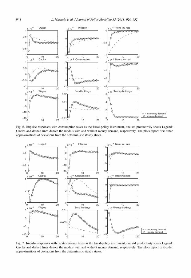
6.1. Impulse response functions
We also calculated impulse response functions – meant as first-order approximation of devia-tions from the deterministic steady state – of selected variables to productivity and money-demandshocks7 under different fiscal policy instruments. They are calculated based on welfare-optimizingparametrization. Figs. 1–7 report the plots, with the upper panel showing the technology shockand the lower panel the monetary one.
7 Obviously the latter involves the presence of a non-zero money demand, whereas in the former we consider bothspecifications.

946 L. Marattin et al. / Journal of Policy Modeling 33 (2011) 920–952
-.3
-.2
-.1
.0
.1
.2
.3
1 2 3 4 5 6 7 8 9 10
Response of deficit to output shock
-.3
-.2
-.1
.0
.1
.2
.3
1 2 3 4 5 6 7 8 9 10
Response of Deficit to Debt shock
Response of Deficit to one st. dev. innovations
Fig. 2. Impulse responses Legend: The error bands are computed according to Antithetic Accelerated Monte-Carlo 10000simulations.
The dashed lines indicate the cashless economy, and the circled lines refer to a positive moneydemand. After a positive technology shock, output and consumption increase under any targetinginstrument, as standard. Inflation decreases and as a result nominal interest rate also decreases,since the feedback coefficient of the monetary policy rule on inflation is bigger that the oneon output. It is interesting to note, in monetary economies, a significant liquidity effect, cap-tured by the relevant increase in money holdings. Kim (2000) and Sims (1998) argue that such astrong liquidity effects is made possible by the substantial amount of nominal and real rigiditiesin the underlying structure of the model. While impulse response function retain the standardqualitative effects under any targeting, we can emphasize the different quantitative responseof endogenous variables which are subject to distortionary taxation. With, alternatively, con-sumption, capital income and wage as fiscal instruments we observe negative effect on the
-.3
-.2
-.1
.0
.1
.2
1 2 3 4 5 6 7 8 9 10
Response of debt to one st. dev. output innovation
Fig. 3. Impulse responses Legend: The error bands are computed according to Antithetic Accelerated Monte-Carlo 10000simulations.

L. Marattin et al. / Journal of Policy Modeling 33 (2011) 920–952 947
0 10 200
0.5
1
1.5x 10
−3 Output
0 10 20−15
−10
−5
0
5x 10
−4 Inflation
0 10 20−15
−10
−5
0
5x 10
−4 Nom. int. rate
0 10 200
2
4
6
8x 10
−4 Capital
0 10 200
1
2
3
4x 10
−3 Consumption
0 10 20−1
−0.5
0
0.5
1x 10
−3 Hours worked
0 10 200
2
4
6x 10
−4 Wages
0 10 20−0.03
−0.02
−0.01
0
0.01Bond holdings
0 10 200
0.005
0.01Money holdings
money demandno money demand
Fig. 4. Impulse responses with lump-sum taxes as the fiscal-policy instrument, one std productivity shock Legend:Circles and dashed lines denote the models with and without money demand, respectively. The plots report first-orderapproximations of deviations from the deterministic steady states.
0 10 20−2
−1
0
1x 10
−3 Output
0 10 20−15
−10
−5
0
5x 10
−4 Inflation
0 10 20−6
−4
−2
0
2x 10
−4 Nom. int. rate
0 10 20−5
0
5
10x 10
−4 Capital
0 10 200
2
4
6x 10
−4 Consumption
0 10 20−3
−2
−1
0
1x 10
−3 Hours worked
0 10 20−10
−5
0
5x 10
−4 Wages
0 10 200
0.005
0.01Bond holdings
0 10 20−5
0
5
10x 10
−4Money holdings
no money demandmoney demand
Fig. 5. Impulse responses with constant steady-state taxation, one std productivity shock Legend: Circles and dashedlines denote the models with and without money demand, respectively. The plots report first-order approximations ofdeviations from the deterministic steadystates.
948 L. Marattin et al. / Journal of Policy Modeling 33 (2011) 920–952
0 10 20−1
−0.5
0
0.5
1x 10
−3 Output
0 10 20−2
−1
0
1x 10
−3 Inflation
0 10 20−1
−0.5
0x 10
−3 Nom. int. rate
0 10 20−1
−0.5
0
0.5
1x 10
−3 Capital
0 10 20−1
0
1
2
3x 10
−3 Consumption
0 10 20−3
−2
−1
0x 10
−3 Hours worked
0 10 20−15
−10
−5
0
5x 10
−4 Wages
0 10 20−0.01
0
0.01
0.02Bond holdings
0 10 200
2
4
6x 10
−3Money holdings
no money demandmoney demand
Fig. 6. Impulse responses with consumption taxes as the fiscal-policy instrument, one std productivity shock Legend:Circles and dashed lines denote the models with and without money demand, respectively. The plots report first-orderapproximations of deviations from the deterministic steady states.
0 10 20−1
−0.5
0
0.5
1x 10
−3 Output
0 10 20−15
−10
−5
0
5x 10
−4 Inflation
0 10 20−10
−5
0
5x 10
−4 Nom. int. rate
0 10 20−5
0
5x 10
−4 Capital
0 10 200
2
4x 10
−4 Consumption
0 10 20−3
−2
−1
0
1x 10
−3 Hours worked
0 10 20−10
−5
0
5x 10
−4 Wages
0 10 200
0.005
0.01Bond holdings
0 10 20−5
0
5
10x 10
−4Money holdings
no money demandmoney demand
Fig. 7. Impulse responses with capital-income taxes as the fiscal-policy instrument, one std productivity shock Legend:Circles and dashed lines denote the models with and without money demand, respectively. The plots report first-orderapproximations of deviations from the deterministic steady states.

L. Marattin et al. / Journal of Policy Modeling 33 (2011) 920–952 949
0 10 200
0.5
1
1.5
2x 10
−3 Output
0 10 20−15
−10
−5
0
5x 10
−4 Inflation
0 10 20−15
−10
−5
0
5x 10
−4 Nom. int. rate
0 10 200
0.5
1x 10
−3 Capital
0 10 200
1
2
3
4x 10
−3 Consumption
0 10 20−1
−0.5
0
0.5
1x 10
−3 Hours worked
0 10 200
2
4
6x 10
−4 Wages
0 10 20−0.04
−0.02
0
0.02Bond holdings
0 10 200
0.005
0.01
0.015Money holdings
no money demandmoney demand
Fig. 8. Impulse responses with labour-income taxes as the fiscal-policy instrument, one std productivity shock Legend:Circles and dashed lines denote the models with and without money demand, respectively. The plots report first-orderapproximations of deviations from the deterministic steady states.
0 10 20−5
0
5x 10
−3 Output
0 10 20−2
−1
0
1x 10
−3 Inflation
0 10 20−2
−1
0
1x 10
−3 Nom. int. rate
0 10 20−2
0
2
4x 10
−3 Capital
0 10 20−2
0
2
4x 10
−3 Consumption
0 10 20−2
0
2
4x 10
−3 Hours worked
0 10 20−1
0
1
2x 10
−3 Wages
0 10 20−0.04
−0.02
0
0.02Bond holdings
0 10 20−5
0
5
10x 10
−3Money holdings
no money demandmoney demand
Fig. 9. Impulse responses with government consumption as the fiscal-policy instrument, one std productivity shockLegend: Circles and dashed lines denote the models with and without money demand, respectively. The plots reportfirst-order approximations of deviations from the deterministic steady states.

950 L. Marattin et al. / Journal of Policy Modeling 33 (2011) 920–952
0 10 20−5
0
5x 10
−3 Output
0 10 20−2
−1
0
1x 10
−3 Inflation
0 10 20−2
−1
0
1x 10
−3 Nom. int. rate
0 10 20−2
0
2
4x 10
−3 Capital
0 10 20−2
0
2
4x 10
−3 Consumption
0 10 20−2
0
2
4x 10
−3 Hours worked
0 10 20−1
0
1
2x 10
−3 Wages
0 10 20−0.04
−0.02
0
0.02Bond holdings
0 10 20−5
0
5
10x 10
−3Money holdings
no money demandmoney demand
Fig. 10. Impulse responses with productive government spending as the fiscal-policy instrument, one std productivityshock Legend: Circles and dashed lines denote the models with and without money demand, respectively. The plots reportfirst-order approximations of deviations from the deterministic steady states.
response of, respectively, aggregate consumption, capital stock and hours worked to the positiveproductivity impulse.
7. Conclusion
In times of pressing need of fiscal consolidation, the relative desiderability of different fiscalpolicy instruments deserves particular attention. We provided statistical evidence that in its firstdecade fiscal policy in the Euro Area has followed a debt-stabilizing approach, reducing primarydeficit after a debt shock. However, whether this stance is welfare maximizing – and, most of all,which side the adjustment should be implemented on – is still an open question. In this paper webuilt a large-scale DSGE model with a considerable number of imperfections and attempted toprovide a welfare comparison of alternative fiscal policy tools according to different monetary pol-icy stances. Consistently with theoretical literature and the real world policy environment, fiscalpolicy targets the accumulation of public debt, by increasing (decreasing) tax rates (governmentspending) in response to fiscal imbalances. Our results show that employing productive govern-ment expenditure as fiscal instrument in the feedback rule on debt is actually Pareto-improvingunder active interest-rate- based monetary policy in a cashless economy. Other instruments – par-ticularly capital income taxation – lead instead to more consistent welfare losses. Modification ofthe economic environment such as non-zero money demand in the cashless economy or moneysupply-based monetary rules still preserve the qualitative properties of our welfare ranking, point-ing towards a relative desirability of productive expenditure-based fiscal adjustments rather thanthe active utilization of distortionary tax instruments.
L. Marattin et al. / Journal of Policy Modeling 33 (2011) 920–952 951
The general validity of such a conclusion might certainly be questioned by a more accurateanalysis, capable of including key aspect that we were forced to leave out here, such a deeperconsideration of the interactions between spending and revenue components of fiscal policy ora more precise investigation of non-Keynesian effects. A possible further step might incorporatesome of the above suggestions so to be able to tackle into a DSGE framework more complex issuessuch as non-linearities in fiscal policy effects of the size of government spending multipliers (Figs.8–10).
References
Alesina, A., & S. Ardagna. (2009). Large changes in fiscal policy: taxes versus spending, unpublished manuscript.Alesina, A., & Perotti, R. (1997). Fiscal adjustments in OECD countries: Composition and macroeconomic effects. IMF
Staff Papers, 44.Anderson, G., Levin, A. T., & Swanson, E. (2004). Higher-order perturbation solutions to dynamic, discrete-time rational
expectations models, unpublished manuscript, Federal Reserve Board.Andrés, J., López-Salido, D., & Vallés, J. (2001). Money in an estimated business cycle model of the Euro area, Bank of
Spain. Working paper, 121.Annichiarico, B. (2007). Government deficits, wealth effects and the price level in an optimizing Euro-model. Journal of
Policy Modeling, 29(1), 15–28.Bayoumi, T., Laxton, D., & Pesenti, P. (2004). Benefits and spillovers of greater competition in Europe, NBER Working
Paper, 10416.Bilbie, F. (2009). Limited asset markets participation, monetary policy and (inverted) keynesian logic, unpublished
manuscript.Blanchard, O. (1985). Debt, deficits and finite horizons. Journal of Political Economy, 93(2), 223–247.Bohn, H. (1995). The sustainability of budget deficits in a stochastic economy. Journal of Money, Credit and Banking,
27, 257–271.Brand, C., & Cassola, N. (2004). A money demand system for Euro area M3. Applied Economics, 36, 817–838.Brand, C., Gerdesmeier, D., & Roffia, B. (2002). Estimating the trend of M3 income velocity underlying the reference
value for monetary growth. ECB Occasional Paper Series, 3.Calvo, G. (1983). Staggered prices in a utility maximizing framework. Journal of Monetary Economics, 12, 383–398.Canzoneri, M., Cumby, R., & Diba, B. (2001). Is the price level determined by the needs of fiscal solvency? American
Economic Review, 91(5), 1221–1238.Chadha, R., & Nolan, C. (2007). Optimal and sRules for the conduct of monetary and fiscal policy. Journal of Macroe-
conomics, 29, 665–689.Davig, T., & Leeper, E. (2005). Fluctuating macro policies and the fiscal theory, unpublished manuscript.Edge, R., & Rudd, J. (2002). Taxation and the Taylor principle, Finance and Economics Discussion Series 51.Galì, J., Lopez-Salido, J., & Vallès, J. (2004). Rule of thumb consumers and the design of interest rate rules. Journal of
Money, Credit and Banking, 36(4), 739–764.Giavazzi, F., & Pagano, M. (1990). Can severe fiscal contractions be expansionary? Tales of two small European countries.
In NBER Macroeconomics Annual MIT Press.Ireland, P. N. (2001). Sticky-price models of the business cycle: Specification and stability. Journal of Monetary Economics.Kim, J. (2003). Functional equivalence between intertemporal and multisectoral investment adjustment costs. Journal of
Economic Dynamics and Control, 27(4), 533–549.Kim, J., & Kim, S. H. (2003). Spurious welfare reversals in international business cycle models. Journal of International
Economics, 60(2), 471–500.Kim, J., & Kim, S. H. (2003b). Welfare effects of tax policy in open economies: Stabilization and cooperation, unpublished
manuscript, Tufts University.Kollmann, R. (2003). Welfare maximizing fiscal and monetary policy rules, unpublished manuscript, University of Bonn.Leeper, E. (1991). Equilibria under ‘Active’ and ‘Passive’ monetary and fiscal policies. Journal of Monetary Economics,
27, 129–147.Leith, C., & Thadden, L. V. (2008). Monetary and fiscal policy interactions in a new Keynesian model with capital
accumulation and non-Ricardian consumers. Journal of Economic Theory, 140(1), 279–313.Leith, C., & Wren-Lewis, S. (2000). Interactions between monetary and fiscal policy rules. Economic Journal, 110,
93–108.
952 L. Marattin et al. / Journal of Policy Modeling 33 (2011) 920–952
Linnemann, L. (2006). Interest rate policy, debt, and indeterminacy with distortionary taxation. Journal of EconomicDynamics and Control, 30, 487–510.
Linnemann, L., & Schabert, A. (2004). Can fiscal spending stimulate private consumption? Economic Letters, 82.Lossani, M., Natale, P., & Tirelli, P. (2003). A nominal income growth target for a conservative ECB? When the policy
mix matters. Journal of Policy Modeling, 25(8), 685–699.Paustian, M. (2003). Gains from second-order approximations, unpublished manuscript, University of Bonn.Prescott, E. C. (2003). Why do Americans work so much more than Europeans?, Staff Report, Federal Reserve Bank of
Minneapolis, 321.Railavo, J. (2004). Stability consequences of fiscal policy rules. Bank of Finland Discussion Paper, 1.Rotemberg, J. (1982). Monopolistic price adjustment and aggregate output. Review of Economic Studies, 49, 517–531.Schmitt-Grohé, S., & Uribe, M. (2004a). Optimal fiscal and monetary policy under imperfect competition, Journal of
Macroeconomics, in press.Schmitt-Grohé, S., & Uribe, M. (2004b). Optimal operational monetary policy in the Christiano-Eichenbaum-Evans model
of the U.S. business cycle, unpublished manuscript, Duke University.Schmitt-Grohé, S., & Uribe, M. (2004). Solving dynamic general equilibrium models using a second-order approximation
to the policy function. Journal of Economic Dynamics and Control, 28(3), 755–775.Schmitt-Grohé, S., & Uribe, M. (2007). Optimal simple and implementable monetary and fiscal rules. Journal of Monetary
Economics, 54, 1702–1725.Sims, C. (1994). A simple model for study of the determination of the price level and the interaction of monetary and
fiscal policy. Economic Theory, 4, 381–399.Sims, C. (1998). The precarious fiscal foundations of EMU, unpublished manuscript, Princeton University.Smets, F., & Wouters, R. (2003). An estimated stochastic dynamic general equilibrium model of the Euro area. Journal
of the European Economic Association, 1(5), 1123–1175.Sutherland, A. (2002). A simple second-order solution method for dynamic general equilibrium models, unpublished
manuscript, University of St Andrews.Tirelli, P. (1992). Simple rules for policy coordination: An evaluation of alternative proposals. Journal of Policy Modeling,
14(1), 1–11.Woodford, M. (1994). Monetary policy and price level determinacy in a cash-in-advance economy. Economic Theory, 25,
345–380.Woodford, M. (2003). Interest and prices: Foundations of a theory of monetary policy. Princeton University Press.