The Annals of Applied Statistics2008, Vol. 2, No. 4, 1360–1383DOI: 10.1214/08-AOAS191© Institute of Mathematical Statistics, 2008

A WEAKLY INFORMATIVE DEFAULT PRIOR DISTRIBUTION FORLOGISTIC AND OTHER REGRESSION MODELS

BY ANDREW GELMAN, ALEKS JAKULIN, MARIA GRAZIA

PITTAU AND YU-SUNG SU

Columbia University, Columbia University, University of Rome, and CityUniversity of New York

We propose a new prior distribution for classical (nonhierarchical) lo-gistic regression models, constructed by first scaling all nonbinary variablesto have mean 0 and standard deviation 0.5, and then placing independentStudent-t prior distributions on the coefficients. As a default choice, werecommend the Cauchy distribution with center 0 and scale 2.5, which inthe simplest setting is a longer-tailed version of the distribution attainedby assuming one-half additional success and one-half additional failure ina logistic regression. Cross-validation on a corpus of datasets shows theCauchy class of prior distributions to outperform existing implementationsof Gaussian and Laplace priors.

We recommend this prior distribution as a default choice for routine ap-plied use. It has the advantage of always giving answers, even when there iscomplete separation in logistic regression (a common problem, even whenthe sample size is large and the number of predictors is small), and also au-tomatically applying more shrinkage to higher-order interactions. This canbe useful in routine data analysis as well as in automated procedures such aschained equations for missing-data imputation.

We implement a procedure to fit generalized linear models in R with theStudent-t prior distribution by incorporating an approximate EM algorithminto the usual iteratively weighted least squares. We illustrate with severalapplications, including a series of logistic regressions predicting voting pref-erences, a small bioassay experiment, and an imputation model for a publichealth data set.

1. Introduction.

1.1. Separation and sparsity in applied logistic regression. Nonidentifiabilityis a common problem in logistic regression. In addition to the problem of collinear-ity, familiar from linear regression, discrete-data regression can also become un-stable from separation, which arises when a linear combination of the predictorsis perfectly predictive of the outcome [Albert and Anderson (1984), Lesaffre andAlbert (1989)]. Separation is surprisingly common in applied logistic regression,

Received January 2008; revised June 2008.Key words and phrases. Bayesian inference, generalized linear model, least squares, hierarchi-

cal model, linear regression, logistic regression, multilevel model, noninformative prior distribution,weakly informative prior distribution.

1360

PRIOR DISTRIBUTION FOR LOGISTIC REGRESSION 1361

especially with binary predictors, and, as noted by Zorn (2005), is often handledinappropriately. For example, a common “solution” to separation is to remove pre-dictors until the resulting model is identifiable, but, as Zorn (2005) points out, thistypically results in removing the strongest predictors from the model.

An alternative approach to obtaining stable logistic regression coefficients is touse Bayesian inference. Various prior distributions have been suggested for thispurpose, most notably a Jeffreys prior distribution [Firth (1993)], but these havenot been set up for reliable computation and are not always clearly interpretable asprior information in a regression context. Here we propose a new, proper prior dis-tribution that produces stable, regularized estimates while still being vague enoughto be used as a default in routine applied work. Our procedure can be seen as a gen-eralization of the scaled prior distribution of Raftery (1996) to the t case, with theadditional innovation that the prior scale parameter is given a direct interpretationin terms of logistic regression parameters.

A simple adaptation of the usual iteratively weighted least squares algorithmallows us to estimate coefficients using independent t prior distributions. This im-plementation works by adding pseudo-data at the least squares step and ensuresnumerical stability of the algorithm—in contrast to existing implementations ofthe Jeffreys prior distribution which can crash when applied to sparse data.

We demonstrate the effectiveness of our method in three applications:(1) a model predicting voting from demographic predictors, which is typical ofmany of our everyday data analyses in political science; (2) a simple bioassaymodel from an early article [Racine et al. (1986)] on routine applied Bayesian in-ference; and (3) a missing-data imputation problem from our current applied workon a study of HIV virus load. None of these applications is technically sophisti-cated; rather, they demonstrate the wide relevance of a default logistic regressionprocedure.

1.2. Relation to existing approaches. Our key idea is to use minimal priorknowledge, specifically that a typical change in an input variable would be unlikelyto correspond to a change as large as 5 on the logistic scale (which would movethe probability from 0.01 to 0.50 or from 0.50 to 0.99). This is related to the “con-ditional means” approach of Bedrick, Christensen, and Johnson (1996) of setting aprior distribution by eliciting the possible distribution of outcomes given differentcombinations of regression inputs, and the method of Witte, Greenland, and Kim(1998) and Greenland (2001) of assigning prior distributions by characterizing ex-pected effects in weakly informative ranges (“probably near null,” “probably mod-erately positive,” etc.). Our method differs from these related approaches in using ageneric prior constraint rather than information specific to a particular analysis. Assuch, we would expect our prior distribution to be more appropriate for automaticuse, with these other methods suggesting ways to add more targeted prior informa-tion when necessary. For example, the conditional means prior is easy to assess andthe posterior is easy to fit, but it is not set up to be applied automatically to a dataset

1362 GELMAN, JAKULIN, PITTAU AND SU

in the way that Jeffreys’ prior—or ours—can be implemented. One approach forgoing further, discussed by MacLehose et al. (2006) and Dunson, Herring, and En-gel (2006), is to use mixture prior distributions for logistic regressions with largenumbers of predictors. These models use batching in the parameters, or attempt todiscover such batching, in order to identify more important predictors and shrinkothers.

Another area of related work is the choice of parametric family for the priordistribution. We have chosen the t family, focusing on the Cauchy as a conserv-ative choice. Genkin, Lewis, and Madigan (2007) consider the Laplace (double-exponential) distribution, which has the property that its posterior mode estimatescan be shrunk all the way to zero. This is an appropriate goal in projects such astext categorization (the application in that article) in which data storage is an is-sue, but is less relevant in social science analysis of data that have already beencollected.

In the other direction, our approach (which, in the simplest logistic regressionthat includes only a constant term, turns out to be close to adding one-half successand one-half failure, as we discuss in Section 2.2) can be seen as a generalizationof the work of Agresti and Coull (1998) on using Bayesian techniques to get pointestimates and confidence intervals with good small-sample frequency properties.As we have noted earlier, similar penalized likelihood methods using the Jeffreysprior have been proposed and evaluated by Firth (1993), Heinze and Schemper(2003), Zorn (2005), and Heinze (2006). Our approach is similar but is parameter-ized in terms of the coefficients and thus allows us to make use of prior knowledgeon that scale. In simple cases the two methods can give similar results (identicalto the first decimal place in the example in Figure 3), with our algorithm beingmore stable by taking advantage of the existing iteratively weighted least squaresalgorithm.

We justify our choice of model and parameters in three ways. First, we inter-pret our prior distribution directly as a constraint on the logistic regression coef-ficients. Second, we show that our default procedure gives reasonable results inthree disparate applications. Third, we borrow an idea from computer science anduse cross-validation on an existing corpus of datasets to compare the predictiveperformance of a variety of prior distributions. The cross-validation points up thenecessity of choosing between the goal of optimal predictions and the statisticalprinciple of conservatism.

2. A default prior specification for logistic regression. There is a vast lit-erature on noninformative, default, and reference prior distributions; see, Jeffreys(1961), Hartigan (1964), Bernardo (1979), Spiegelhalter and Smith (1982), Yangand Berger (1994), and Kass and Wasserman (1996). Our approach differs frommost of this work in that we want to include some actual prior information, enoughto regularize the extreme inferences that are obtained using maximum likelihoodor completely noninformative priors. The existing literature [including, we must

PRIOR DISTRIBUTION FOR LOGISTIC REGRESSION 1363

admit, Gelman et al. (2003)] offers the extremes of (a) fully informative prior dis-tributions using application-specific information, or (b) noninformative priors, typ-ically motivated by invariance principles. Our goal here is something in between:a somewhat informative prior distribution that can nonetheless be used in a widerange of applications. As always with default models, our prior can be viewed asa starting point or placeholder—a baseline on top of which the user can add realprior information as necessary. For this purpose, we want something better thanthe unstable estimates produced by the current default—maximum likelihood (orBayesian estimation with a flat prior).

On the one hand, scale-free prior distributions such as Jeffreys’ do not includeenough prior information; on the other, what prior information can be assumed fora generic model? Our key idea is that actual effects tend to fall within a limitedrange. For logistic regression, a change of 5 moves a probability from 0.01 to 0.5,or from 0.5 to 0.99. We rarely encounter situations where a shift in input x corre-sponds to the probability of outcome y changing from 0.01 to 0.99, hence, we arewilling to assign a prior distribution that assigns low probabilities to changes of 10on the logistic scale.

2.1. Standardizing input variables to a commonly-interpretable scale. A chal-lenge in setting up any default prior distribution is getting the scale right: for ex-ample, suppose we are predicting vote preference given age (in years). We wouldnot want the same prior distribution if the age scale were shifted to months. Butdiscrete predictors have their own natural scale (most notably, a change of 1 in abinary predictor) that we would like to respect.

The first step of our model is to standardize the input variables, a procedure thathas been applied to Bayesian generalized linear models by Raftery (1996) and thatwe have formalized as follows [Gelman (2008)]:

• Binary inputs are shifted to have a mean of 0 and to differ by 1 in their lowerand upper conditions. (For example, if a population is 10% African-Americanand 90% other, we would define the centered “African-American” variable totake on the values 0.9 and −0.1.)

• Other inputs are shifted to have a mean of 0 and scaled to have a standard devia-tion of 0.5. This scaling puts continuous variables on the same scale as symmet-ric binary inputs (which, taking on the values ±0.5, have standard deviation 0.5).

Following Gelman and Pardoe (2007), we distinguish between regression inputsand predictors. For example, in a regression on age, sex, and their interaction, thereare four predictors (the constant term, age, sex, and age × sex), but just two inputs:age and sex. It is the input variables, not the predictors, that are standardized.

A prior distribution on standardized variables depends on the data, but this is notnecessarily a bad idea. As pointed out by Raftery (1996), the data, or “the broadpossible range of the variables,” are relevant to knowledge about the coefficients.If we do not standardize at all, we have to worry about coefficients of very large

1364 GELMAN, JAKULIN, PITTAU AND SU

or very small variables (for example, distance measured in millimeters, meters, orkilometers). One might follow Greenland, Schlesselman, and Criqui (2002) andrequire of users that they put each variable on a reasonable scale before fitting amodel. Realistically, though, users routinely fit regressions on unprocessed data,and we want our default procedure to perform reasonably in such settings.

2.2. A weakly informative t family of prior distributions. The second step ofthe model is to define prior distributions for the coefficients of the predictors. Wefollow Raftery (1996) and assume prior independence of the coefficients as a de-fault assumption, with the understanding that the model could be reparameterizedif there are places where prior correlation is appropriate. For each coefficient, weassume a Student-t prior distribution with mean 0, degrees-of-freedom parame-ter ν, and scale s, with ν and s chosen to provide minimal prior information toconstrain the coefficients to lie in a reasonable range. We are motivated to con-sider the t family because flat-tailed distributions allow for robust inference [see,Berger and Berliner (1986), Lange, Little, and Taylor (1989)], and, as we shall seein Section 3, it allows easy and stable computation in logistic regression by placingiteratively weighted least squares within an approximate EM algorithm. Computa-tion with a normal prior distribution is even easier (no EM algorithm is needed),but we prefer the flexibility of the t family.

Before discussing our choice of parameters, we briefly discuss some limitingcases. Setting the scale s to infinity corresponds to a flat prior distribution (sothat the posterior mode is the maximum likelihood estimate). As we illustrate inSection 4.1, the flat prior fails in the case of separation. Setting the degrees offreedom ν to infinity corresponds to the Gaussian distribution. As we illustrate inSection 5, we obtain better average performance by using a t with finite degrees offreedom (see Figure 6).1 We suspect that the Cauchy prior distribution outperformsthe normal, on average, because it allows for occasional large coefficients whilestill performing a reasonable amount of shrinkage for coefficients near zero; thisis another way of saying that we think the set of true coefficients that we mightencounter in our logistic regressions has a distribution less like a normal than likea Cauchy, with many small values and occasional large ones.

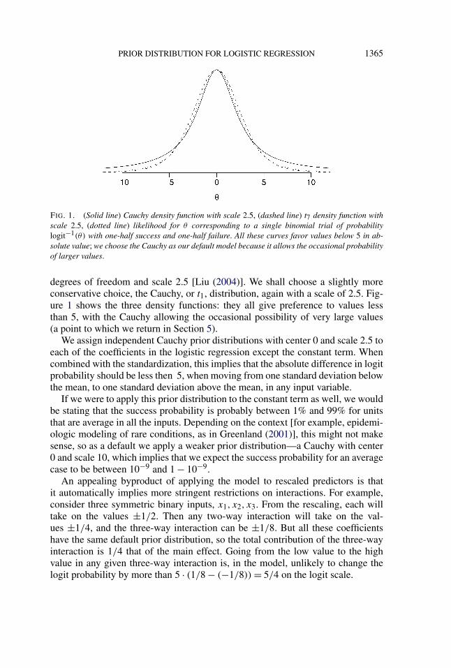
One way to pick a default value of ν and s is to consider the baseline case of one-half of a success and one-half of a failure for a single binomial trial with probabilityp = logit−1(θ)—that is, a logistic regression with only a constant term. The corre-sponding likelihood is eθ/2/(1 + eθ ), which is close to a t density function with 7

1In his discussion of default prior distributions for generalized linear models, Raftery (1996) workswith the Gaussian family and writes that “the results depend little on the precise functional form.”One reason that our recommendations differ in their details from Raftery’s is that we are interestedin predictions and inferences within a single model, with a particular interest in sparse data settingswhere the choice of prior distribution can make a difference. In contrast, Raftery’s primary interest inhis 1996 paper lay in the effect of the prior distribution on the marginal likelihood and its implicationsfor the Bayes factor as used in model averaging.

PRIOR DISTRIBUTION FOR LOGISTIC REGRESSION 1365

FIG. 1. (Solid line) Cauchy density function with scale 2.5, (dashed line) t7 density function withscale 2.5, (dotted line) likelihood for θ corresponding to a single binomial trial of probabilitylogit−1(θ) with one-half success and one-half failure. All these curves favor values below 5 in ab-solute value; we choose the Cauchy as our default model because it allows the occasional probabilityof larger values.

degrees of freedom and scale 2.5 [Liu (2004)]. We shall choose a slightly moreconservative choice, the Cauchy, or t1, distribution, again with a scale of 2.5. Fig-ure 1 shows the three density functions: they all give preference to values lessthan 5, with the Cauchy allowing the occasional possibility of very large values(a point to which we return in Section 5).

We assign independent Cauchy prior distributions with center 0 and scale 2.5 toeach of the coefficients in the logistic regression except the constant term. Whencombined with the standardization, this implies that the absolute difference in logitprobability should be less then 5, when moving from one standard deviation belowthe mean, to one standard deviation above the mean, in any input variable.

If we were to apply this prior distribution to the constant term as well, we wouldbe stating that the success probability is probably between 1% and 99% for unitsthat are average in all the inputs. Depending on the context [for example, epidemi-ologic modeling of rare conditions, as in Greenland (2001)], this might not makesense, so as a default we apply a weaker prior distribution—a Cauchy with center0 and scale 10, which implies that we expect the success probability for an averagecase to be between 10−9 and 1 − 10−9.

An appealing byproduct of applying the model to rescaled predictors is thatit automatically implies more stringent restrictions on interactions. For example,consider three symmetric binary inputs, x1, x2, x3. From the rescaling, each willtake on the values ±1/2. Then any two-way interaction will take on the val-ues ±1/4, and the three-way interaction can be ±1/8. But all these coefficientshave the same default prior distribution, so the total contribution of the three-wayinteraction is 1/4 that of the main effect. Going from the low value to the highvalue in any given three-way interaction is, in the model, unlikely to change thelogit probability by more than 5 · (1/8 − (−1/8)) = 5/4 on the logit scale.

1366 GELMAN, JAKULIN, PITTAU AND SU

3. Computation. In principle, logistic regression with our prior distributioncan be computed using the Gibbs and Metropolis algorithms. We do not give de-tails as this is now standard with Bayesian models; see, for example, Carlin andLouis (2001), Martin and Quinn (2002), and Gelman et al. (2003). In practice,however, it is desirable to have a quick calculation that returns a point estimate ofthe regression coefficients and standard errors. Such an approximate calculationworks in routine statistical practice and, in addition, recognizes the approximatenature of the model itself.

We consider three computational settings:

• Classical (nonhierarchical) logistic regression, using our default prior distribu-tion in place of the usual flat prior distribution on the coefficients.

• Multilevel (hierarchical) modeling, in which some of the default prior distri-bution is applied only to the subset of the coefficients that are not otherwisemodeled (sometimes called the “fixed effects”).

• Chained imputation, in which each variable with missing data is modeled condi-tional on the other variables with a regression equation, and these models are fitand random imputations inserted iteratively [Van Buuren and Oudshoom (2000),Raghunathan, Van Hoewyk, and Solenberger (2001)].

In any of these cases, our default prior distribution has the purpose of stabilizing(regularizing) the estimates of otherwise unmodeled parameters. In the first sce-nario, the user typically only extracts point estimates and standard errors. In thesecond scenario, it makes sense to embed the computation within the full Markovchain simulation. In the third scenario of missing-data imputation, we would likethe flexibility of quick estimates for simple problems with the potential for Markovchain simulation as necessary. Also, because of the automatic way in which thecomponent models are fit in a chained imputation, we would like a computation-ally stable algorithm that returns reasonable answers.

We have implemented these computations by altering the glm function in R,creating a new function, bayesglm, that finds an approximate posterior mode andvariance using extensions of the classical generalized linear model computations,as described in the rest of this section. The bayesglm function (part of the armpackage for applied regression and multilevel modeling in R) allows the user tospecify independent prior distributions for the coefficients in the t family, withthe default being Cauchy distributions with center 0 and scale set to 10 (for theregression intercept), 2.5 (for binary predictors), or 2.5/(2 · sd), where sd is thestandard deviation of the predictor in the data (for other numerical predictors).We are also extending the program to fit hierarchical models in which regressioncoefficients are structured in batches [Gelman et al. (2008)].

3.1. Incorporating the prior distribution into classical logistic regression com-putations. Working in the context of the logistic regression model,

Pr(yi = 1) = logit−1(Xiβ),(1)

PRIOR DISTRIBUTION FOR LOGISTIC REGRESSION 1367

we adapt the classical maximum likelihood algorithm to obtain approximate pos-terior inference for the coefficients β , in the form of an estimate β̂ and covariancematrix Vβ .

The standard logistic regression algorithm—upon which we build—proceedsby approximately linearizing the derivative of the log-likelihood, solving usingweighted least squares, and then iterating this process, each step evaluating thederivatives at the latest estimate β̂; see, for example, McCullagh and Nelder(1989). At each iteration, the algorithm determines pseudo-data zi and pseudo-variances (σ z

i )2 based on the linearization of the derivative of the log-likelihood,

zi = Xiβ̂ + (1 + eXiβ̂)2

eXiβ̂

(yi − eXiβ̂

1 + eXiβ̂

),

(σ zi )2 = 1

ni

(1 + eXiβ̂ )2

eXiβ̂,(2)

and then performs weighted least squares, regressing z on X with weight vector(σ z)−2. The resulting estimate β̂ is used to update the computations in (2), and theiteration proceeds until approximate convergence.

Computation with a specified normal prior distribution. The simplest informa-tive prior distribution assigns normal prior distributions for the components of β:

βj ∼ N(μj , σ2j ) for j = 1, . . . , J.(3)

This information can be effortlessly included in the classical algorithm by simplyaltering the weighted least-squares step, augmenting the approximate likelihoodwith the prior distribution; see, for example, Section 14.8 of Gelman et al. (2003).If the model has J coefficients βj with independent N(μj , σ

2j ) prior distributions,

then we add J pseudo-data points and perform weighted linear regression on “ob-servations” z∗, “explanatory variables” X∗, and weight vector w∗, where

z∗ =(

z

μ

), X∗ =

(X

IJ

), w∗ = (σ z, σ )−2.(4)

The vectors z∗,w∗, and the matrix X∗ are constructed by combining the likelihood[z and σz, are the vectors of zi ’s and σz

i ’s defined in (2), and X is the design matrixof the regression (1)] and the prior [μ and σ are the vectors of μj ’s and σj ’sin (3), and IJ is the J × J identity matrix]. As a result, z∗ and w∗ are vectorsof length n+J and X∗ is an (n+J ) × J matrix. With the augmented X∗, thisregression is identified, and, thus, the resulting estimate β̂ is well defined and hasfinite variance, even if the original data have collinearity or separation that wouldresult in nonidentifiability of the maximum likelihood estimate.

The full computation is then iteratively weighted least squares, starting with aguess of β (for example, independent draws from the unit normal distribution),

1368 GELMAN, JAKULIN, PITTAU AND SU

then computing the derivatives of the log-likelihood to compute z and σz, thenusing weighted least squares on the pseudo-data (4) to yield an updated estimateof β , then recomputing the derivatives of the log-likelihood at this new value ofβ , and so forth, converging to the estimate β̂ . The covariance matrix Vβ is simplythe inverse second derivative matrix of the log-posterior density evaluated at β̂—that is, the usual normal-theory uncertainty estimate for an estimate not on theboundary of parameter space.

Approximate EM algorithm with a t prior distribution. If the coefficients βj

have independent t prior distributions2 with centers μj and scales sj , we can adaptthe just-described iteratively weighted least squares algorithm to estimate the co-efficients using an approximate EM algorithm (Dempster, Laird and Rubin 1977).We shall describe the steps of the algorithm shortly; the idea is to express the t

prior distribution for each coefficient βj as a mixture of normals with unknownscale σj :

βj ∼ N(μj , σ2j ), σ 2

j ∼ Inv -χ2(νj , s2j )(5)

and then average over the βj ’s at each step, treating them as missing data andperforming the EM algorithm to estimate the σj ’s. The algorithm proceeds byalternating one step of iteratively weighted least squares (as described above) andone step of EM. Once enough iterations have been performed to reach approximateconvergence, we get an estimate and covariance matrix for the vector parameter β

and the estimated σj ’s.We initialize the algorithm by setting each σj to the value sj (the scale of the

prior distribution) and, as before, starting with a guess of β (either obtained froma simpler procedure or simply picking a starting value such as β = 0). Then, ateach step of the algorithm, we update σ by maximizing the expected value of its(approximate) log-posterior density,

logp(β,σ |y) ≈ −1

2

n∑i=1

1

(σ zi )2 (zi − Xiβ)2

− 1

2

J∑j=1

(1

σ 2j

(βj − μj)2 + log(σ 2

j )

)

− p(σj |νj , sj ) + constant.(6)

Each iteration of the algorithm proceeds as follows:

2As discussed earlier, we use the default settings μj = 0, sj = 2.5, νj = 1 (except for the constantterm, if any, to whose prior distributions we assign the parameters μj = 0, sj = 10, νj = 1), but wedescribe the computation more generally in terms of arbitrary values of these parameters.

PRIOR DISTRIBUTION FOR LOGISTIC REGRESSION 1369

1. Based on the current estimate of β , perform the normal approximation to thelog-likelihood and determine the vectors z and σz using (2), as in classicallogistic regression computation.

2. Approximate E-step: first run the weighted least squares regression based onthe augmented data (4) to get an estimate β̂ with variance matrix Vβ . Thendetermine the expected value of the log-posterior density by replacing the terms(βj − μj)

2 in (6) by

E((βj − μj)

2|σ, y) ≈ (β̂j − μj)

2 + (Vβ)jj ,(7)

which is only approximate because we are averaging over a normal distributionthat is only an approximation to the generalized linear model likelihood.

3. M-step: maximize the (approximate) expected value of the log-posterior density(6) to get the estimate,

σ̂ 2j = (β̂j − μj)

2 + (Vβ)jj + νj s2j

1 + νj

,(8)

which corresponds to the (approximate) posterior mode of σ 2j given a single

measurement with value (7) and an Inv-χ2(νj , s2j ) prior distribution.

4. Recompute the derivatives of the log-posterior density given the current β̂ , setup the augmented data (4) using the estimated σ̂ from (8), and repeat steps 1,2, 3 above.

At convergence of the algorithm, we summarize the inferences using the latestestimate β̂ and covariance matrix Vβ .

3.2. Other models.

Linear regression. Our algorithm is basically the same for linear regression,except that weighted least squares is an exact rather than approximate maximumpenalized likelihood, and also a step needs to be added to estimate the data vari-ance. In addition, we would preprocess y by rescaling the outcome variable tohave mean 0 and standard deviation 0.5 before assigning the prior distribution (or,equivalently, multiply the prior scale parameter by the standard deviation of thedata). Separation is not a concern in linear regression; however, when applied rou-tinely (for example, in iterative imputation algorithms), collinearity can arise, inwhich case it is helpful to have a proper but weak prior distribution.

Other generalized linear models. Again, the basic algorithm is unchanged, ex-cept that the pseudo-data and pseudo-variances in (2), which are derived from thefirst and second derivatives of the log-likelihood, are changed [see Section 16.4of Gelman et al. (2003)]. For Poisson regression and other models with the log-arithmic link, we would not often expect effects larger than 5 on the logarithmic

1370 GELMAN, JAKULIN, PITTAU AND SU

scale, and so the prior distributions given in this article might be a reasonabledefault choice. In addition, for models such as the negative binomial that havedispersion parameters, these can be estimated using an additional step as is donewhen estimating the data-level variance in normal linear regression. For more com-plex models such as multinomial logit and probit, we have considered combiningindependent t prior distributions on the coefficients with pseudo-data to identifycutpoints in the possible presence of sparse data. Such models also present compu-tational challenges, as there is no simple existing iteratively weighted least squaresalgorithm for us to adapt.

Avoiding nested looping when inserting into larger models. In multilevel mod-els [Gelman et al. (2008)] or in applications such as chained imputation (discussedin Section 4.3), it should be possible to speed the computation by threading, ratherthan nesting, the loops. For example, suppose we are fitting an imputation by iter-atively regressing u on v,w, then v on u,w, then w on u, v. Instead of doing a fulliterative weighted least squares at each iteration, then we could perform one stepof weighted least squares at each step, thus taking less computer time to ultimatelyconverge by not wasting time by getting hyper-precise estimates at each step of thestochastic algorithm.

4. Applications.

4.1. A series of regressions predicting vote preferences. Regular users of lo-gistic regression know that separation can occur in routine data analyses, evenwhen the sample size is large and the number of predictors is small. The leftcolumn of Figure 2 shows the estimated coefficients for logistic regression pre-dicting the probability of a Republican vote for president for a series of elections.The estimates look fine except in 1964, where there is complete separation, with allthe African-American respondents supporting the Democrats. Fitting in R actuallyyields finite estimates, as displayed in the graph, but these are essentially meaning-less, being a function of how long the iterative fitting procedure goes before givingup.

The other three columns of Figure 2 show the coefficient estimates using ourdefault Cauchy prior distribution for the coefficients, along with the t7 and normaldistributions. (In all cases, the prior distributions are centered at 0, with scale pa-rameters set to 10 for the constant term and 2.5 for all other coefficients.) All threeprior distributions do a reasonable job at stabilizing the estimated coefficient forrace for 1964, while leaving the estimates for other years essentially unchanged.This example illustrates how we could use our Bayesian procedure in routine prac-tice.

PRIOR DISTRIBUTION FOR LOGISTIC REGRESSION 1371

FIG. 2. The left column shows the estimated coefficients (±1 standard error) for a logistic regres-sion predicting the probability of a Republican vote for president given sex, race, and income, as fitseparately to data from the National Election Study for each election 1952 through 2000. [The binaryinputs female and black have been centered to have means of zero, and the numerical variableincome (originally on a 1–5 scale) has been centered and then rescaled by dividing by two standarddeviations.]There is complete separation in 1964 (with none of the black respondents supporting the Republicancandidate, Barry Goldwater), leading to a coefficient estimate of −∞ that year. (The particular finitevalues of the estimate and standard error are determined by the number of iterations used by the glmfunction in R before stopping.)The other columns show estimated coefficients (±1 standard error) for the same model fit each yearusing independent Cauchy, t7, and normal prior distributions, each with center 0 and scale 2.5. Allthree prior distributions do a reasonable job at stabilizing the estimates for 1964, while leaving theestimates for other years essentially unchanged.

4.2. A small bioassay experiment. We next consider a small-sample examplein which the prior distribution makes a difference for a coefficient that is already

1372 GELMAN, JAKULIN, PITTAU AND SU

Dose, xi Number of Number of

(log g/ml) animals, ni deaths, yi

−0.86 5 0

−0.30 5 1

−0.05 5 3

0.73 5 5

# from glm:coef.est coef.se

(Intercept) -0.1 0.7z.x 10.2 6.4n = 4, k = 2residual deviance = 0.1, null deviance = 15.8 (difference = 15.7)

# from bayesglm (Cauchy priors, scale 10 for const and 2.5 for other coef):coef.est coef.se

(Intercept) -0.2 0.6z.x 5.4 2.2n = 4, k = 2residual deviance = 1.1, null deviance = 15.8 (difference = 14.7)

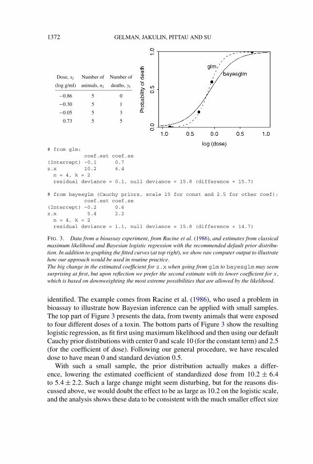
FIG. 3. Data from a bioassay experiment, from Racine et al. (1986), and estimates from classicalmaximum likelihood and Bayesian logistic regression with the recommended default prior distribu-tion. In addition to graphing the fitted curves (at top right), we show raw computer output to illustratehow our approach would be used in routine practice.The big change in the estimated coefficient for z.x when going from glm to bayesglm may seemsurprising at first, but upon reflection we prefer the second estimate with its lower coefficient for x,which is based on downweighting the most extreme possibilities that are allowed by the likelihood.

identified. The example comes from Racine et al. (1986), who used a problem inbioassay to illustrate how Bayesian inference can be applied with small samples.The top part of Figure 3 presents the data, from twenty animals that were exposedto four different doses of a toxin. The bottom parts of Figure 3 show the resultinglogistic regression, as fit first using maximum likelihood and then using our defaultCauchy prior distributions with center 0 and scale 10 (for the constant term) and 2.5(for the coefficient of dose). Following our general procedure, we have rescaleddose to have mean 0 and standard deviation 0.5.

With such a small sample, the prior distribution actually makes a differ-ence, lowering the estimated coefficient of standardized dose from 10.2 ± 6.4to 5.4 ± 2.2. Such a large change might seem disturbing, but for the reasons dis-cussed above, we would doubt the effect to be as large as 10.2 on the logistic scale,and the analysis shows these data to be consistent with the much smaller effect size

PRIOR DISTRIBUTION FOR LOGISTIC REGRESSION 1373

of 5.4. The large amount of shrinkage simply confirms how weak the informationis that gave the original maximum likelihood estimate. The graph at the upper rightof Figure 3 shows the comparison in a different way: the maximum likelihood es-timate fits the data almost perfectly; however, the discrepancies between the dataand the Bayes fit are small, considering the sample size of only 5 animals withineach group.3

4.3. A set of chained regressions for missing-data imputation. Multiple im-putation [Rubin (1978, 1996)] is another context in which regressions with manypredictors are fit in an automatic way. It is common to have missing data in sev-eral variables in an analysis, in which case one cannot simply set up a model fora single partially-observed outcome given a set of fully-observed predictors. Moregenerally, we must think of the dataset as a multivariate outcome, any componentsof which can be missing. The direct approach to imputing missing data in severalvariables is to fit a multivariate model. However, this approach requires a lot ofeffort to set up a reasonable multivariate regression model and a fully specifiedjoint model is sometime difficult to specify, particularly when we have a mixtureof different types of variables.

A different approach, becoming more popular for imputing missing data,uses chained equations [Van Buuren and Oudshoom (2000), Raghunathan, VanHoewyk, and Solenberger (2001)], a series of conditional distributions without theneed to fit a multivariate model. In chained imputation, each variable is imputedusing a regression model conditional on all the others, iteratively cycling throughall the variables that contain missing data. Different models can be specified fordifferent variables to be imputed, and logistic regression is a natural choice forbinary variables. When the number of variables is large, separation can arise. Ourprior distribution yields stable computations in this setting, as we illustrate in anexample from our current applied research.

We consider a model from our current applied research imputing virus loads ina longitudinal sample of HIV-positive homeless persons. The analysis incorporatesa large number of predictors, including demographic and health-related variables,and often with high rates of missingness. Inside the multiple imputation chainedequation procedure, logistic regression is used to impute the binary variables. It isgenerally recommended to include a rich set of predictors when imputing missingvalues [Rubin (1996)]. However, in this application, including all the dichotomouspredictors leads to many instances of separation.

To take one example from our analysis, separation arose when estimating eachperson’s probability of attendance in a group therapy called haart. The toppart of Figure 4 shows the model as estimated using the glm function in R

3For example, the second data point (log(x) = −0.30) has an empirical rate of 1/5 = 0.20 and apredicted probability (from the Bayes fit) of 0.27. With a sample size of 5, we could expect a standarderror of

√0.27 · (1 − 0.27)/5 = 0.20, so a difference of 0.07 should be of no concern.

1374 GELMAN, JAKULIN, PITTAU AND SU

# from glm:coef.est coef.sd coef.est coef.sd

(Intercept) 0.07 1.41 h39b.W1 -0.10 0.03age.W1 0.02 0.02 pcs.W1 -0.01 0.01mcs37.W1 -0.01 0.32 nonhaartcombo.W1 -20.99 888.74unstabl.W1 -0.09 0.37 b05.W1 -0.07 0.12ethnic.W3 -0.14 0.23 h39b.W2 0.02 0.03age.W2 0.02 0.02 pcs.W2 -0.01 0.02mcs37.W2 0.26 0.31 haart.W2 1.80 0.30nonhaartcombo.W2 1.33 0.44 unstabl.W2 0.27 0.42b05.W2 0.03 0.12 h39b.W3 0.00 0.03age.W3 -0.01 0.02 pcs.W3 0.01 0.01mcs37.W3 -0.04 0.32 haart.W3 0.60 0.31nonhaartcombo.W3 0.44 0.42 unstabl.W3 -0.92 0.40b05.W3 -0.11 0.11

# from bayesglm (Cauchy priors, scale 10 for constand 2.5 for other coefs):

coef.est coef.sd coef.est coef.sd(Intercept) -0.84 1.15 h39b.W1 -0.08 0.03age.W1 0.01 0.02 pcs.W1 -0.01 0.01mcs37.W1 -0.10 0.31 nonhaartcombo.W1 -6.74 1.22unstabl.W1 -0.06 0.36 b05.W1 0.02 0.12ethnic.W3 0.18 0.21 h39b.W2 0.01 0.03age.W2 0.03 0.02 pcs.W2 -0.02 0.02mcs37.W2 0.19 0.31 haart.W2 1.50 0.29nonhaartcombo.W2 0.81 0.42 unstabl.W2 0.29 0.41b05.W2 0.11 0.12 h39b.W3 -0.01 0.03age.W3 -0.02 0.02 pcs.W3 0.01 0.01mcs37.W3 0.05 0.32 haart.W3 1.02 0.29nonhaartcombo.W3 0.64 0.40 unstabl.W3 -0.52 0.39b05.W3 -0.15 0.13

FIG. 4. A logistic regression fit for missing-data imputation using maximum likelihood (top) andBayesian inference with default prior distribution (bottom). The classical fit resulted in an error mes-sage indicating separation; in contrast, the Bayes fit (using independent Cauchy prior distributionswith mean 0 and scale 10 for the intercept and 2.5 for the other coefficients) produced stable esti-mates. We would not usually summarize results using this sort of table, however, this gives a sense ofhow the fitted models look in routine data analysis.

fit to the observed cases in the first year of the data set: the coefficient fornonhaartcombo.W1 is essentially infinity, and the regression also gives an er-ror message indicating nonidentifiability. The bottom part of Figure 4 shows the fitusing our recommended Bayesian procedure (this time, for simplicity, not recen-tering and rescaling the inputs, most of which are actually binary).

In the chained imputation, the classical glm fits were nonidentifiable at manyplaces; none of these presented any problem when we switched to our newbayesglm function.4

4We also tried the brlr and brglm functions in R, which implement the Jeffreys prior dis-tributions of Firth (1993) and Kosimidis (2007). Unfortunately, we still encountered problems in

PRIOR DISTRIBUTION FOR LOGISTIC REGRESSION 1375

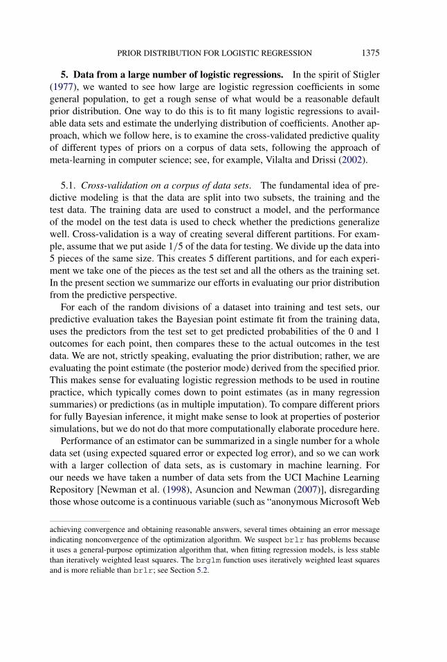
5. Data from a large number of logistic regressions. In the spirit of Stigler(1977), we wanted to see how large are logistic regression coefficients in somegeneral population, to get a rough sense of what would be a reasonable defaultprior distribution. One way to do this is to fit many logistic regressions to avail-able data sets and estimate the underlying distribution of coefficients. Another ap-proach, which we follow here, is to examine the cross-validated predictive qualityof different types of priors on a corpus of data sets, following the approach ofmeta-learning in computer science; see, for example, Vilalta and Drissi (2002).

5.1. Cross-validation on a corpus of data sets. The fundamental idea of pre-dictive modeling is that the data are split into two subsets, the training and thetest data. The training data are used to construct a model, and the performanceof the model on the test data is used to check whether the predictions generalizewell. Cross-validation is a way of creating several different partitions. For exam-ple, assume that we put aside 1/5 of the data for testing. We divide up the data into5 pieces of the same size. This creates 5 different partitions, and for each experi-ment we take one of the pieces as the test set and all the others as the training set.In the present section we summarize our efforts in evaluating our prior distributionfrom the predictive perspective.

For each of the random divisions of a dataset into training and test sets, ourpredictive evaluation takes the Bayesian point estimate fit from the training data,uses the predictors from the test set to get predicted probabilities of the 0 and 1outcomes for each point, then compares these to the actual outcomes in the testdata. We are not, strictly speaking, evaluating the prior distribution; rather, we areevaluating the point estimate (the posterior mode) derived from the specified prior.This makes sense for evaluating logistic regression methods to be used in routinepractice, which typically comes down to point estimates (as in many regressionsummaries) or predictions (as in multiple imputation). To compare different priorsfor fully Bayesian inference, it might make sense to look at properties of posteriorsimulations, but we do not do that more computationally elaborate procedure here.

Performance of an estimator can be summarized in a single number for a wholedata set (using expected squared error or expected log error), and so we can workwith a larger collection of data sets, as is customary in machine learning. Forour needs we have taken a number of data sets from the UCI Machine LearningRepository [Newman et al. (1998), Asuncion and Newman (2007)], disregardingthose whose outcome is a continuous variable (such as “anonymous Microsoft Web

achieving convergence and obtaining reasonable answers, several times obtaining an error messageindicating nonconvergence of the optimization algorithm. We suspect brlr has problems becauseit uses a general-purpose optimization algorithm that, when fitting regression models, is less stablethan iteratively weighted least squares. The brglm function uses iteratively weighted least squaresand is more reliable than brlr; see Section 5.2.

1376 GELMAN, JAKULIN, PITTAU AND SU

Name Cases Num Cat Pred Outcome Pr(y = 1) Pr(NA) |�x|mushroom 8124 0 22 95 edible=e 0.52 0 3.0spam 4601 57 0 105 class=0 0.61 0 3.2krkp 3196 0 36 37 result=won 0.52 0 2.6segment 2310 19 0 154 y=5 0.14 0 3.5titanic 2201 0 3 5 surv=no 0.68 0 0.7car 1728 0 6 15 eval=unacc 0.70 0 2.0cmc 1473 2 7 19 Contracept=1 0.43 0 1.9german 1000 7 13 48 class=1 0.70 0 2.8tic-tac-toe 958 0 9 18 y=p 0.65 0 2.3heart 920 7 6 30 num=0 0.45 0.15 2.3anneal 898 6 32 64 y=3 0.76 0.65 2.4vehicle 846 18 0 58 Y=3 0.26 0 3.0pima 768 8 0 11 class=0 0.65 0 1.8crx 690 6 9 45 A16=- 0.56 0.01 2.3australian 690 6 8 36 Y=0 0.56 0 2.3soybean-large 683 35 0 75 y=brown-spot 0.13 0.10 3.2breast-wisc-c 683 9 0 20 y=2 0.65 0 1.6balance-scale 625 0 4 16 name=L 0.46 0 1.8monk2 601 0 6 11 y=0 0.66 0 1.9wdbc 569 20 0 45 diag=B 0.63 0 3.0monk1 556 0 6 11 y=0 0.50 0 1.9monk3 554 0 6 11 y=1 0.52 0 1.9voting 435 0 16 32 party=dem 0.61 0 2.7horse-colic 369 7 19 121 outcom=1 0.61 0.20 3.4ionosphere 351 32 0 110 y=g 0.64 0 3.5bupa 345 6 0 6 selector=2 0.58 0 1.5primary-tumor 339 0 17 25 primary=1 0.25 0.04 2.0ecoli 336 7 0 12 y=cp 0.43 0 1.3breast-LJ-c 286 3 6 16 recurrence=no 0.70 0.01 1.8shuttle-control 253 0 6 10 y=2 0.57 0 1.8audiology 226 0 69 93 y=cochlear-age 0.25 0.02 2.3glass 214 9 0 15 y=2 0.36 0 1.7yeast-class 186 79 0 182 func=Ribo 0.65 0.02 4.6wine 178 13 0 24 Y=2 0.40 0 2.2hayes-roth 160 0 4 11 y=1 0.41 0 1.5hepatitis 155 6 13 35 Class=LIVE 0.79 0.06 2.5iris 150 4 0 8 y=virginica 0.33 0 1.6lymphography 148 2 16 29 y=2 0.55 0 2.5promoters 106 0 57 171 y=mm 0.50 0 6.1zoo 101 1 15 17 type=mammal 0.41 0 2.2post-operative 88 1 7 14 ADM-DECS=A 0.73 0.01 1.6soybean-small 47 35 0 22 y=D4 0.36 0 2.6lung-cancer 32 0 56 103 y=2 0.41 0 4.3lenses 24 0 4 5 lenses=none 0.62 0 1.4o-ring-erosion 23 3 0 4 no-therm-d=0 0.74 0 0.7

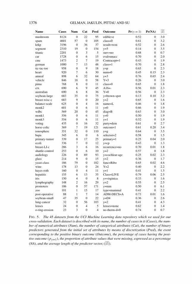
FIG. 5. The 45 datasets from the UCI Machine Learning data repository which we used for ourcross-validation. Each dataset is described with its name, the number of cases in it (Cases), the num-ber of numerical attributes (Num), the number of categorical attributes (Cat), the number of binarypredictors generated from the initial set of attributes by means of discretization (Pred), the eventcorresponding to the positive binary outcome (Outcome), the percentage of cases having the posi-tive outcome (py=1), the proportion of attribute values that were missing, expressed as a percentage

(NA), and the average length of the predictor vector, (|�x|).

PRIOR DISTRIBUTION FOR LOGISTIC REGRESSION 1377

data”) and those that are given in the form of logical theories (such as “artificialcharacters”). Figure 5 summarized the datasets we used for our cross-validation.

Because we do not want our results to depend on an imputation method, wetreat missingness as a separate category for each variable for which there are miss-ing cases: that is, we add an additional predictor for each variable with missingdata indicating whether the particular predictor’s value is missing. We also use theFayyad and Irani (1993) method for converting continuous predictors into discreteones. To convert a k-level predictor into a set of binary predictors, we create k − 1predictors corresponding to all levels except the most frequent. Finally, for all datasets with multinomial outcomes, we transform into binary by simply comparingthe most frequent category to the union of all the others.

5.2. Average predictive errors corresponding to different prior distributions.We use fivefold cross-validation to compare “bayesglm” (our approximate Bayespoint estimate) for different default scale and degrees of freedom parameters; recallthat degrees of freedom equal 1 and ∞ for the Cauchy and Gaussian prior distribu-tions, respectively. We also compare to three existing methods: (1) the “glm” func-tion in R that fits classical logistic regression (equivalent to bayesglm with priorscale set to ∞); (2) the “brglm” implementation of Jeffreys’ prior from Kosmidis(2007), with logit and probit links; and (3) the BBR (Bayesian binary regression)algorithm of Genkin, Lewis, and Madigan (2007), which adaptively sets the scalefor the choice of Laplacian or Gaussian prior distribution.

In comparing with glm, we had a practical constraint. When no finite maxi-mum likelihood estimate exists, we define the glm solution as that obtained by theR function using its default starting value and default number of iterations.

Figure 6 shows the results, displaying average logarithmic and Brier score lossesfor different choices of prior distribution.5 The Cauchy prior distribution with scale0.75 performs best, on average. Classical logistic regression (“glm”), which corre-sponds to prior degrees of freedom and prior scale both set to ∞, did not do well:with no regularization, maximum likelihood occasionally gives extreme estimates,which then result in large penalties in the cross-validation. In fact, the log and Brierscores for classical logistic regression would be even worse except that the glmfunction in R stops after a finite number of iterations, thus giving estimates that are

5Given the vector of predictors �x, the true outcome y and the predicted probability py = f (�x)

for y, the Brier score is defined as (1 − py)2/2 and the logarithmic score is defined as − logpy .Because of cross-validation, the probabilities were built without using the predictor-outcome pairs(�x, y), so we are protected against overfitting. Miller, Hui, and Tierney (1990) and Jakulin and Bratko(2003) discuss the use of scores to summarize validation performance in logistic regression.

Maximizing the Brier score [Brier (1950)] is equivalent to minimizing mean square error, andmaximizing the logarithmic score is equivalent to maximizing the likelihood of the out-of-sampledata. Both these rules are “proper” in the sense of being maximized by the true probability, if themodel is indeed true [Winkler (1969)].

1378 GELMAN, JAKULIN, PITTAU AND SU

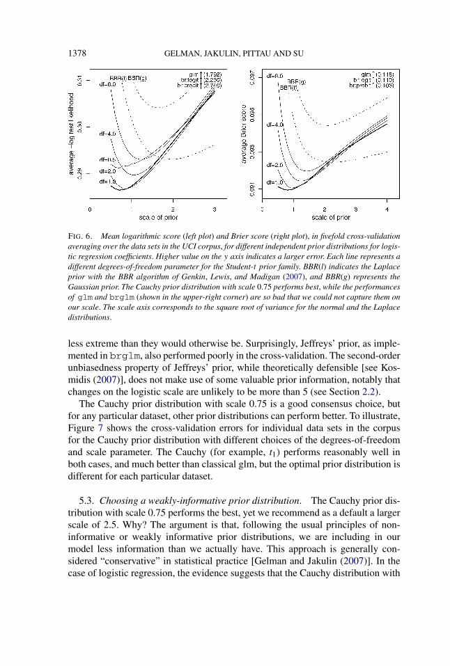
FIG. 6. Mean logarithmic score (left plot) and Brier score (right plot), in fivefold cross-validationaveraging over the data sets in the UCI corpus, for different independent prior distributions for logis-tic regression coefficients. Higher value on the y axis indicates a larger error. Each line represents adifferent degrees-of-freedom parameter for the Student-t prior family. BBR(l) indicates the Laplaceprior with the BBR algorithm of Genkin, Lewis, and Madigan (2007), and BBR(g) represents theGaussian prior. The Cauchy prior distribution with scale 0.75 performs best, while the performancesof glm and brglm (shown in the upper-right corner) are so bad that we could not capture them onour scale. The scale axis corresponds to the square root of variance for the normal and the Laplacedistributions.

less extreme than they would otherwise be. Surprisingly, Jeffreys’ prior, as imple-mented in brglm, also performed poorly in the cross-validation. The second-orderunbiasedness property of Jeffreys’ prior, while theoretically defensible [see Kos-midis (2007)], does not make use of some valuable prior information, notably thatchanges on the logistic scale are unlikely to be more than 5 (see Section 2.2).

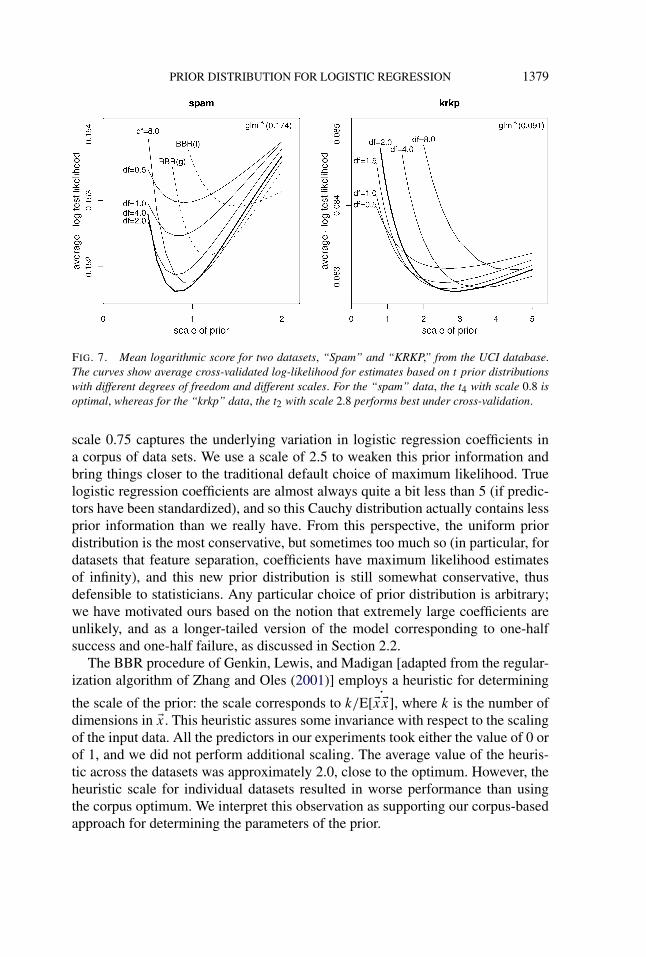
The Cauchy prior distribution with scale 0.75 is a good consensus choice, butfor any particular dataset, other prior distributions can perform better. To illustrate,Figure 7 shows the cross-validation errors for individual data sets in the corpusfor the Cauchy prior distribution with different choices of the degrees-of-freedomand scale parameter. The Cauchy (for example, t1) performs reasonably well inboth cases, and much better than classical glm, but the optimal prior distribution isdifferent for each particular dataset.

5.3. Choosing a weakly-informative prior distribution. The Cauchy prior dis-tribution with scale 0.75 performs the best, yet we recommend as a default a largerscale of 2.5. Why? The argument is that, following the usual principles of non-informative or weakly informative prior distributions, we are including in ourmodel less information than we actually have. This approach is generally con-sidered “conservative” in statistical practice [Gelman and Jakulin (2007)]. In thecase of logistic regression, the evidence suggests that the Cauchy distribution with

PRIOR DISTRIBUTION FOR LOGISTIC REGRESSION 1379

FIG. 7. Mean logarithmic score for two datasets, “Spam” and “KRKP,” from the UCI database.The curves show average cross-validated log-likelihood for estimates based on t prior distributionswith different degrees of freedom and different scales. For the “spam” data, the t4 with scale 0.8 isoptimal, whereas for the “krkp” data, the t2 with scale 2.8 performs best under cross-validation.

scale 0.75 captures the underlying variation in logistic regression coefficients ina corpus of data sets. We use a scale of 2.5 to weaken this prior information andbring things closer to the traditional default choice of maximum likelihood. Truelogistic regression coefficients are almost always quite a bit less than 5 (if predic-tors have been standardized), and so this Cauchy distribution actually contains lessprior information than we really have. From this perspective, the uniform priordistribution is the most conservative, but sometimes too much so (in particular, fordatasets that feature separation, coefficients have maximum likelihood estimatesof infinity), and this new prior distribution is still somewhat conservative, thusdefensible to statisticians. Any particular choice of prior distribution is arbitrary;we have motivated ours based on the notion that extremely large coefficients areunlikely, and as a longer-tailed version of the model corresponding to one-halfsuccess and one-half failure, as discussed in Section 2.2.

The BBR procedure of Genkin, Lewis, and Madigan [adapted from the regular-ization algorithm of Zhang and Oles (2001)] employs a heuristic for determining

the scale of the prior: the scale corresponds to k/E[ ·�x �x], where k is the number ofdimensions in �x. This heuristic assures some invariance with respect to the scalingof the input data. All the predictors in our experiments took either the value of 0 orof 1, and we did not perform additional scaling. The average value of the heuris-tic across the datasets was approximately 2.0, close to the optimum. However, theheuristic scale for individual datasets resulted in worse performance than usingthe corpus optimum. We interpret this observation as supporting our corpus-basedapproach for determining the parameters of the prior.

1380 GELMAN, JAKULIN, PITTAU AND SU

6. Discussion. We recommend using, as a default prior model, independentCauchy distributions on all logistic regression coefficients, each centered at 0 andwith scale parameter 10 for the constant term and 2.5 for all other coefficients.Before fitting this model, we center each binary input to have mean 0 and rescaleeach numeric input to have mean 0 and standard deviation 0.5. When applyingthis procedure to classical logistic regression, we fit the model using an adaptationof the standard iteratively weighted least squares computation, using the posteriormode as a point estimate and the curvature of the log-posterior density to get stan-dard errors. More generally, the prior distribution can be used as part of a fullyBayesian computation in more complex settings such as hierarchical models.

A theoretical concern with our method is that the prior distribution is definedon centered and scaled input variables, thus, it implicitly depends on the data.As more data arrive, the linear transformations used in the centering and scalingwill change, thus changing the implied prior distribution as defined on the orig-inal scale of the data. A natural extension here would be to formally make theprocedure hierarchical, for example, defining the j th input variable xij as hav-ing a population mean μj and standard deviation σj , then defining the prior dis-tributions for the corresponding predictors in terms of scaled inputs of the formzij = (xij − μj)/(2σj ). We did not go this route, however, because modeling allthe input variables corresponds to a potentially immense effort which is contraryto the spirit of this method, which is to be a quick automatic solution. In practice,we do not see the dependence of our prior distribution on data as a major con-cern, although we imagine it could cause difficulties when sample sizes are verysmall.

Modeling the coefficient of a scaled variable is analogous to parameterizing asimple regression through the correlation, which depends on the distribution ofx as well as the regression of y on x. Changing the values of x can change thecorrelation, and thus the implicit prior distribution, even though the regression isnot changing at all (assuming an underlying linear relationship). That said, thisis the cost of having an informative prior distribution: some scale must be used,and the scale of the data seems like a reasonable default choice. No model can beuniversally applied: in many settings it will make more sense to use a more infor-mative prior distribution based on subject-matter knowledge; in other cases, whereparameters might plausibly take on any value, a noninformative prior distributionmight be appropriate.

Finally, one might argue that the Bayesian procedure, by always giving an esti-mate, obscures nonidentifiability and could lead the user into a false sense of se-curity. To this objection, we would reply [following Zorn (2005)] as follows: first,one is always free to also fit using maximum likelihood, and second, separationcorresponds to information in the data, which is ignored if the offending predictoris removed and awkward to handle if it is included with an infinite coefficient (see,for example, the estimates for 1964 in the first column of Figure 2). Given that wedo not expect to see effects as large as 10 on the logistic scale, it is appropriate to

PRIOR DISTRIBUTION FOR LOGISTIC REGRESSION 1381

use this information. As we have seen in specific examples and also in the corpusof datasets, this weakly-informative prior distribution yields estimates that makemore sense and perform better predictively, compared to maximum likelihood,which is still the standard approach for routine logistic regression in theoreticaland applied statistics.

Acknowledgments. We thank Chuanhai Liu, David Dunson, Hal Stern, Davidvan Dyk, and editors and referees for helpful comments, Peter Messeri for the HIVexample, David Madigan for help with the BBR software, Ioannis Kosimidis forhelp with the brglm software, Masanao Yajima for help in developing bayesglm,and the National Science Foundation, National Institutes of Health, and ColumbiaUniversity Applied Statistics Center for financial support.

REFERENCES

AGRESTI, A. and COULL, B. A. (1998). Approximate is better than exact for interval estimation ofbinomial proportions. Amer. Statist. 52 119–126.MR1628435

ALBERT, A. and ANDERSON, J. A. (1984). On the existence of maximum likelihood estimates inlogistic regression models. Biometrika 71 1–10. MR0738319

ASUNCION, A. and NEWMAN, D. J. (2007). UCI Machine Learning Repository.Dept. of Information and Computer Sciences, Univ. California, Irvine. Available atwww.ics.uci.edu/~mlearn/MLRepository.html.

BEDRICK, E. J., CHRISTENSEN, R. and JOHNSON, W. (1996). A new perspective on priors forgeneralized linear models. J. Amer. Statist. Assoc. 91 1450–1460. MR1439085

BERGER, J. O. and BERLINER, L. M. (1986). Robust Bayes and empirical Bayes analysis withepsilon-contaminated priors. Ann. Statist. 14 461–486. MR0840509

BERNARDO, J. M. (1979). Reference posterior distributions for Bayesian inference (with discus-sion). J. Roy. Statist. Soc. Ser. B 41 113–147. MR0547240

BRIER, G. W. (1950). Verification of forecasts expressed in terms of probability. Monthly WeatherReview 78 1–3.

CARLIN, B. P. and LOUIS, T. A. (2001). Bayes and Empirical Bayes Methods for Data Analysis,2nd ed. CRC Press. London.

DEMPSTER, A. P., LAIRD, N. M. and RUBIN, D. B. (1977). Maximum likelihood from incompletedata via the EM algorithm (with discussion). J. Roy. Statist. Soc. Ser. B 39 1–38. MR0501537

DUNSON, D. B., HERRING, A. H. and ENGEL, S. M. (2006). Bayesian selection and clustering ofpolymorphisms in functionally-related genes. J. Amer. Statist. Assoc. To appear.

FAYYAD, U. M. and IRANI, K. B. (1993). Multi-interval discretization of continuous-valued at-tributes for classification learning. In Proceedings of the International Joint Conference on Arti-ficial Intelligence IJCAI-93. Morgan Kauffman, Chambery, France.

FIRTH, D. (1993). Bias reduction of maximum likelihood estimates. Biometrika 80 27–38.MR1225212

GELMAN, A. (2008). Scaling regression inputs by dividing by two standard deviations. Statist. Med.To appear.

GELMAN, A., CARLIN, J. B., STERN, H. S. and RUBIN, D. B. (2003). Bayesian Data Analysis,2nd ed. CRC Press, London. MR2027492

GELMAN, A. and JAKULIN, A. (2007). Bayes: Liberal, radical, or conservative? Statist. Sinica 17422–426. MR2435285

GELMAN, A. and PARDOE, I. (2007). Average predictive comparisons for models with nonlinearity,interactions, and variance components. Sociological Methodology.

1382 GELMAN, JAKULIN, PITTAU AND SU

GELMAN, A., PITTAU, M. G., YAJIMA, M. and SU, Y. S. (2008). An approximate EM algorithmfor multilevel generalized linear models. Technical report, Dept. of Statistics, Columbia Univ.

GENKIN, A., LEWIS, D. D. and MADIGAN, D. (2007). Large-scale Bayesian logistic regression fortext categorization. Technometrics 49 291–304. MR2408634

GREENLAND, S. (2001). Putting background information about relative risks into conjugate priordistributions. Biometrics 57 663–670. MR1863443

GREENLAND, S., SCHLESSELMAN, J. J. and CRIQUI, M. H. (2002). The fallacy of employingstandardized regression coefficients and correlations as measures of effect. American Journal ofEpidemiology 123 203–208.

HARTIGAN, J. (1964). Invariant prior distributions. Ann. Math. Statist. 35 836–845. MR0161406HEINZE, G. (2006). A comparative investigation of methods for logistic regression with separated

or nearly separated data. Statist. Med. 25 4216–4226. MR2307586HEINZE, G. and SCHEMPER, M. (2003). A solution to the problem of separation in logistic regres-

sion. Statist. Med. 12 2409–2419.JAKULIN, A. and BRATKO, I. (2003). Analyzing attribute dependencies. In Knowledge Discovery

in Databases: PKDD 2003 229–240.JEFFREYS, H. (1961). Theory of Probability, 3rd ed. Oxford Univ. Press. MR0187257KASS, R. E. and WASSERMAN, L. (1996). The selection of prior distributions by formal rules.

J. Amer. Statist. Assoc. 91 1343–1370.KOSMIDIS, I. (2007). Bias reduction in exponential family nonlinear models. Ph.D. thesis, Dept. of

Statistics, Univ. Warwick, England.LESAFFRE, E. and ALBERT, A. (1989). Partial separation in logistic discrimination. J. Roy. Statist.

Soc. Ser. B 51 109–116. MR0984997LANGE, K. L., LITTLE, R. J. A. and TAYLOR, J. M. G. (1989). Robust statistical modeling using

the t distribution. J. Amer. Statist. Assoc. 84 881–896. MR1134486LIU, C. (2004). Robit regression: A simple robust alternative to logistic and probit regression. In

Applied Bayesian Modeling and Causal Inference from Incomplete-Data Perspectives (A. Gelmanand X. L. Meng, eds.) 227–238. Wiley, London. MR2138259

MACLEHOSE, R. F., DUNSON, D. B., HERRING, A. H. and HOPPIN, J. A. (2006). Bayesianmethods for highly correlated exposure data. Epidemiology. To appear.

MARTIN, A. D. and QUINN, K. M. (2002). MCMCpack. Available at mcmcpack.wush.edu.MCCULLAGH, P. and NELDER, J. A. (1989). Generalized Linear Models, 2nd ed. Chapman and

Hall, London. MR0727836MILLER, M. E., HUI, S. L. and TIERNEY, W. M. (1990). Validation techniques for logistic regres-

sion models. Statist. Med. 10 1213–1226.NEWMAN, D. J., HETTICH, S., BLAKE, C. L. and MERZ, C. J. (1998). UCI Repository of machine

learning databases. Dept. of Information and Computer Sciences, Univ. California, Irvine.RACINE, A., GRIEVE, A. P., FLUHLER, H. and SMITH, A. F. M. (1986). Bayesian methods in

practice: Experiences in the pharmaceutical industry (with discussion). Appl. Statist. 35 93–150.MR0868007

RAFTERY, A. E. (1996). Approximate Bayes factors and accounting for model uncertainty in gener-alised linear models. Biometrika 83 251–266. MR1439782

RAGHUNATHAN, T. E., VAN HOEWYK, J. and SOLENBERGER, P. W. (2001). A multivariatetechnique for multiply imputing missing values using a sequence of regression models. Surv.Methodol. 27 85–95.

RUBIN, D. B. (1978). Multiple imputations in sample surveys: A phenomenological Bayesian ap-proach to nonresponse (with discussion). In Proc. Amer. Statist. Assoc., Survey Research MethodsSection 20–34.

RUBIN, D. B. (1996). Multiple imputation after 18+ years (with discussion). J. Amer. Statist. Assoc.91 473–520.

PRIOR DISTRIBUTION FOR LOGISTIC REGRESSION 1383

SPIEGELHALTER, D. J. and SMITH, A. F. M. (1982). Bayes factors for linear and log-linear modelswith vague prior information. J. Roy. Statist. Soc. Ser. B 44 377–387. MR0693237

STIGLER, S. M. (1977). Do robust estimators work with real data? Ann. Statist. 5 1055–1098.MR0455205

VAN BUUREN, S. and OUDSHOOM, C. G. M. (2000). MICE: Multivariate imputa-tion by chained equations (S software for missing-data imputation). Available atweb.inter.nl.net/users/S.van.Buuren/mi/.

VILALTA, R. and DRISSI, Y. (2002). A perspective view and survey of metalearning. ArtificialIntelligence Review 18 77–95.

WINKLER, R. L. (1969). Scoring rules and the evaluation of probability assessors. J. Amer. Statist.Assoc. 64 1073–1078.

WITTE, J. S., GREENLAND, S. and KIM, L. L. (1998). Software for hierarchical modeling of epi-demiologic data. Epidemiology 9 563–566.

ZHANG, T. and OLES, F. J. (2001). Text categorization based on regularized linear classificationmethods. Information Retrieval 4 5–31.

YANG, R. and BERGER, J. O. (1994). Estimation of a covariance matrix using reference prior. Ann.Statist. 22 1195–1211. MR1311972

ZORN, C. (2005). A solution to separation in binary response models. Political Analysis 13 157–170.

A. GELMAN

DEPARTMENT OF STATISTICS

AND DEPARTMENT OF POLITICAL SCIENCE

COLUMBIA UNIVERSITY

NEW YORK

USAE-MAIL: gelman@stat.columbia.eduURL: WWW.STAT.COLUMBIA.EDU/~GELMAN

A. JAKULIN

DEPARTMENT OF STATISTICS

COLUMBIA UNIVERSITY

NEW YORK

USA

M. G. PITTAU

DEPARTMENT OF ECONOMICS

UNIVERSITY OF ROME

ITALY

Y.-S. SU

DEPARTMENT OF POLITICAL SCIENCE

CITY UNIVERSITY OF NEW YORK

USA