A Visualization Approach to the Principles of Classical ... · Classical Lagrangian/Hamiltonian...

© Wing Kam Liu, Eduard G. Karpov,Harold Park, David Farrell, Dept. of Mechanical Engineering, Northwestern University, 1

A Visualization Approach to the Principles of Classical Lagrangian/Hamiltonian Mechanics

and its Relations to Molecular Dynamics


Reading Assignment

• H. Goldstein, Classical mechanics, 2nd ed., 1980 (3rd ed., 2002), pages 1-21, 35-45, 339-347.

• L. D. Landau, E. M. Lifshitz, Mechanics, 3rd ed. reprinted since 1976 till 1995, pages 1-10, 131-133.

• J.M. Haile, Molecular Dynamics Simulation, Wiley, 2002, pages 46-59, 188-204, 224-234, 277-282.


Particles (Material Mass Points)

Particle, or material point, or mass point is a mathematical model of a body whose dimensions can be neglected in describing its motion.

Particle is a dimensionless object having a non-zero mass.

Particle is indestructible; it has no internal structure and no internal degrees of freedoms.

Classical mechanics studies “slow” (v << c) and “heavy” (m >> me) particles.

Examples:

1) Planets of the solar system in their motion about the sun

2) Atoms of a gas in a macroscopic vessel

Note: Spherical objects are typically treated as material points, e.g. atoms comprising a molecule. The material point points are associated with the centers of the spheres. Characteristic physical dimensions of the spheres are modeled through particle-particle interaction.


Generalized Coordinates

Generalized coordinates are given by a minimum set of independent parameters (distances and angles) that determine any given state of the system.

Standard coordinate systems are Cartesian, polar, elliptic, cylindrical and spherical.Other systems of coordinates can also be chosen. We will look for a basic form of the equation which is invariant for all coordinate systems.

1 2( , ,..., )sq q q

Examples:

Material point in xy-plane Pendulum Sliding suspension pendulum

We are looking for a basic form of equation motion, which is valid for all coordinate systems.

y

xj j

x

1 2,q x q y= = 1q ϕ=1 2,q x q ϕ= =


Least Action (Hamilton’s) Principle

Lagrange function (Lagrangian)

Action integral

Trajectory variation

Least action, or Hamilton’s, principle

2

1

( , , ) 0t

t

S L q q t dtδ δ= =∫

1 2 1 2( , ,..., , , ,..., , )s sL q q q q q q t

,a b a cS S S S< <

2( )q t

1( )q t

bS

aS cS

1tt

2t

( )q t

2

1

( , , )t

t

S L q q t dt= ∫

1 2( ) ( ), ( ) ( ) 0q t q t q t q tδ δ δ+ = =

Action is minimum along the true trajectory:

The main task of classical dynamics is to find the true trajectories (laws of motion) for all degrees of freedom in the system.


Lagrangian Equation of Motion

Lagrange function (Lagrangian)

Least action principle

2

1

( , , ) 0t

t

S L q q t dtδ δ= =∫

0, 1, 2,...,d L L sdt q qα α

α∂ ∂− = =

∂ ∂

1 2 1 2( , ,..., ; , ,..., , )s sL q q q q q q t

Lagrangian equation is based on the least action principle only, and it is valid for all coordinate systems.

Substitution of the Lagrange function into the action integral with further application of the least action principle yields the Lagrangian equation motion:


Summary of the Lagrangian Method

1. The choice of s generalized coordinates (s – number of degrees of freedom).

2. Derivation of the kinetic and potential energy in terms of the generalized coordinates

3. The difference between the kinetic and potential energies gives the Lagrangian function.

4. Substitution of the Lagrange function into the Lagrangian equation of motion and derivation of a system of s second-order differential equations to be solved.

5. Solution of the equations of motion, using a numerical time-integration algorithm.

6. Post-processing and visualization.


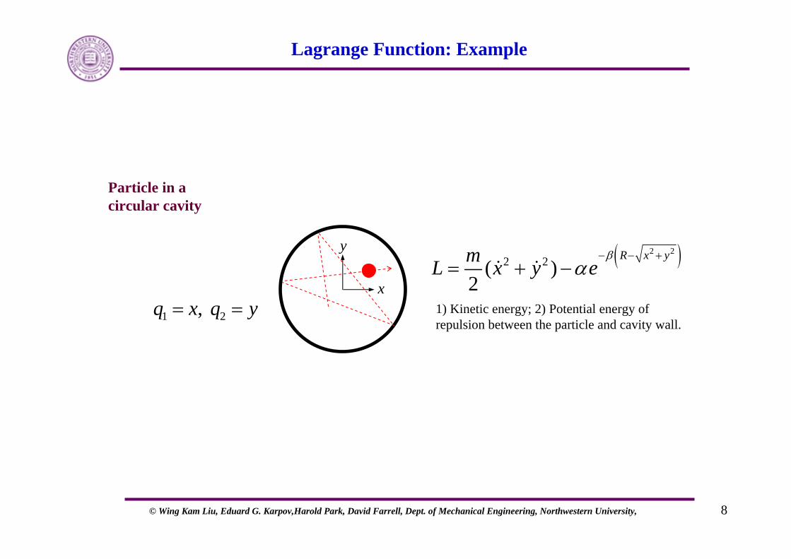
Lagrange Function: Example

Particle in a circular cavity

( )2 22 2( )

2R x ymL x y e

βα

− − += + −

1) Kinetic energy; 2) Potential energy of repulsion between the particle and cavity wall.

y

x

1 2,q x q y= =


Particle in a Circular Cavity: Lagrange Function Derivation

( , ) ( , )L T x y U x y= −General form

Kinetic energy

Potential energy

The total Lagrangian

2 2( )2mT x y= +

( ) ( )2 2R x yR rU e eββα α

− − +− −= =

The potential energy grows quickly and becomes larger than the typical kinetic energy, when the distance r between the particle and the center of the cavity approaches value R.

R is the effective radius of the cavity. At r < R, U does not alter the trajectory.

β is a relative scaling factor: the potential energy growths in eβ times between r = R and r = R+1.

( )2 22 2( , , , ) ( )

2R x ymL x y x y x y e

βα

− − += + −

y

xr

R


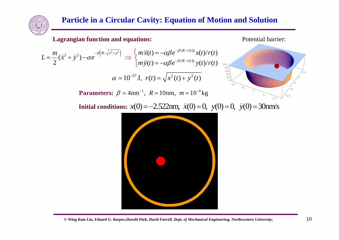
Particle in a Circular Cavity: Equation of Motion and Solution

Lagrangian function and equations: Potential barrier:

(0) 2.522nm, (0) 0, (0) 0, (0) 30nm/sx x y y=− = = =

27 2 210 J, ( ) ( ) ( )r t x t y tα −= = +

1 94nm , 10nm, 10 kgR mβ − −= = =Parameters:

Initial conditions:

( )2 2 ( ( ))2 2

( ( ))

( ) ( )/ ( )( )

2 ( ) ( )/ ( )

R r tR x y

R r t

m x t e x t r tmL x y emy t e y t r t

ββ

β

αβα

αβ

− −− − +

− −

⎧ = −= + −

−⇒ ⎨

=⎩


Predictable and Chaotic Systems

Divergence of trajectoriesin predictable systems

Divergence of trajectoriesin chaotic (unpredictable) systems

Trajectories in MD systems are unpredictable/unstable; they are characterized by a random dependence on initial conditions.

( ) ( ) ( ), (0) : , (0) , (0)q q t q q t q q t q C tδ= + +∼

( ) ( ) ( ), (0) : , (0) , (0) tq q t q q t q q t q eλδ δ= + +∼

Variance of the trajectory depends linearly on time

Variance of the trajectory depends exponentially on time (J.M. Haile, Molecular Dynamics Simulation, 2002)


Example Quasiperiodic System: Particle in a Circular Cavity

Initial conditions

(0) nm, (0) 0(0) 0, (0) 10 nm/s

x xy y

= == =−2.522 (0) nm, (0) 0

(0) 0, (0) 10 nm/sx xy y

= == =−2.500

Dependence of solutions on initial conditions is smooth and predictable in stable systems.


Example Unstable System: Discontinuous Boundary

Initial conditions

(0) nm, (0) 0(0) 0, (0) 10 nm/s

x xy y

= == =−2.522 (0) nm, (0) 0

(0) 0, (0) 10 nm/sx xy y

= == =−2.500

No predictable dependence on initial conditions exists in unstable systems.


Transition from Stable to Chaotic Motion: Example

Initial conditions

1 2

1 2

1.55rad(0) 1.9rad, (0)(0) (0) 0

ϕ ϕϕ ϕ

= == =

1 2 0.6ml l= =

1 2

1 2

1.7rad(0) 1.9rad, (0)(0) (0) 0

ϕ ϕϕ ϕ= =

= =

Note the transition from a stable to chaotic motion (small variance of initial conditions may lead to qualitative change of solution behavior of the same non-linear system).

Periodic motion Chaotic motion


Molecular Dynamics (MD)

A computer simulation technique• Time evolution of interacting atoms pursued by integrating the corresponding equations of motion in time

Based on the Newtonian classical dynamics

Method received widespread attention in the 1970`s• Digital computer become powerful and affordable


Molecular Dynamics Today

• Liquids• Allows the study of new systems, elemental and multicomponent• Investigation of transport phenomena i.e. viscosity and heat flow

• Defects in crystals• Improved realism due to better potentials constitutes a driving force

• Fracture• Provides insight into mechanisms and speeds of fracture process

• Surfaces• Helps understand surface reconstructing, surface melting,

faceting, surface diffusion, roughening, etc.

• Friction• Atomic force microscope• Investigates adhesion and friction between two solids

-and others-


MD System

• Subdomain of a macroscale object

• Manipulated and controlled by the environment via interactions

• Various kinds of boundaries and interactions are possible

• We consider:

• Adiabatically isolated systems that can exchange neither matter nor energy with their surroundings• Non-isolated systems that can exchange heat with the surrounding media (the heat bath, and the multiscale boundary conditions developed at Northwestern)


Summary of the MD Simulation Procedure

• Model individual particles and boundaries.

• Model interaction between particles and between particles and boundaries.

• Assign initial positions and velocities.

• Solve the equations of motion.

• Simulate the movements of the system.

• Analyze the simulation data to investigate collective phenomena and behavior of macroscopic parameters.

Essence of MD:

To solve numerically the N-body problem of classical mechanics


Newtonian Dynamics

Molecular forces and positions change with time.

In principle, an MD simulation is a solution of a system of Newtonian equations of motion.

The Newtonian equation (the Newton’s second law) is a special case of the Lagrangian equation of motion for mass points in a Cartesiansystem.

For such a system, the Lagrangian function is given by

( ) ( )

2 2 2

1 2

( ) ( )2, ,... , , ,

ii i i

i

i i i i

mL x y z U

x y z

= + + −

= =

∑ r

r r r r

X

Y

Z

ri

rj

rij


Newtonian Dynamics

By utilizing the Lagrangian equation of motion at qα= xi, qα+1= yi, qα+2= zi,

( ), , ,( ), , ,i i i i x i y i z ii

Um F F F ∂= = = −

∂rF r F

r

1 1 2 2

, ,

0, 0, 0

, , i i x i i i y i

d L L d L L d L Ldt q q dt q q dt q q

m x F m y F

α α α α α α+ + + +

∂ ∂ ∂ ∂ ∂ ∂− = − = − =

∂ ∂ ∂ ∂ ∂ ∂

⇓ ⇓ ⇓= = , i i z im z f=

This can be rewritten in the vector form:


Interatomic Potential

The most general form of the potential is given by the series

The one-body potential W1 describes external force fields (e.g. gravitational filed), and external constraining fields (e.g. the “wall function” for particles in a circular chamber)

The two-body potential describes dependence of the potential energy on the distances between pairs of atoms in the system:

The three-body and higher order potentials (often ignored)provide dependence on the geometry of atomic

arrangement/bonding.For instance, a dependence on the angle between three mass points is given by

1 2 1 2 3, , ,

( , ,..., ) ( ) ( , ) ( , , ) ...N i i j i j ki i j i i j i k j

U W W W> > >

= + + +∑ ∑ ∑r r r r r r r r r

2 2( , ) ( ), | | | |i j ij i jW W r r= = = −r r r r rx

y

z

rj

rij

ri

i

j

3 3( , , ) (cos ), cos| | | |

ji jki j k ijk ijk

ji jk

W W θ θ⋅

= =r r

r r rr r x

y

z

rj rk

θijk

i

k

j

rji

rjk


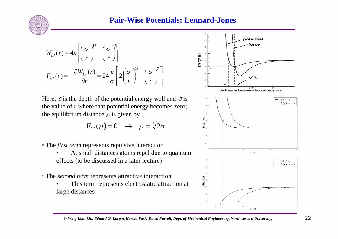
Pair-Wise Potentials: Lennard-Jones

12 6

13 7

( ) 4

( )( ) 24 2

LJ

LJLJ

W rr r

W rF rr r r

σ σε

ε σ σσ

⎡ ⎤⎛ ⎞ ⎛ ⎞= −⎢ ⎥⎜ ⎟ ⎜ ⎟⎝ ⎠ ⎝ ⎠⎢ ⎥⎣ ⎦

⎡ ⎤∂ ⎛ ⎞ ⎛ ⎞= − = −⎢ ⎥⎜ ⎟ ⎜ ⎟∂ ⎝ ⎠ ⎝ ⎠⎢ ⎥⎣ ⎦

6( ) 0 2LJF ρ ρ σ= → =

Here, ε is the depth of the potential energy well and σ is the value of r where that potential energy becomes zero; the equilibrium distance ρ is given by

• The first term represents repulsive interaction • At small distances atoms repel due to quantum effects (to be discussed in a later lecture)

• The second term represents attractive interaction • This term represents electrostatic attraction at large distances


Periodic Boundary Conditions

Simulated system encompasses boundary conditions

Periodic Boundary conditions for particles in a box • Box replicated to infinity in all three Cartesian directions;

Motivation for periodic boundary conditions: domain reduction and analysis of a representative substructure only.

Particles in all boxes move simultaneously, though only one modeled explicitly, i.e. represented in the computer code • Each particle interacts with other particles in the box and with images in

nearby boxes • Interactions occur also through the boundaries • No surface effects take place


Periodic Boundary Conditions: Example

Example simulation of an atomic cluster with periodic boundary conditions.A particles, going through a boundaries returns to the box from the opposite side:

This model is equivalent to a larger system, comprised of the translation image boxes:


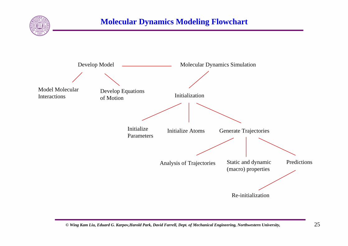
Molecular Dynamics Modeling Flowchart

Develop Model Molecular Dynamics Simulation

Model Molecular Interactions

Develop Equations of Motion

Generate Trajectories

Analysis of Trajectories

Initialization

Static and dynamic (macro) properties

Predictions

Initialize Parameters

Initialize Atoms

Re-initialization


Post-Processing

After simulation is completed, macroscopic properties of the system are evaluated based on (microscopic) atomic positions and velocities:

1. Macroscopic thermodynamic parameters- temperature- internal energy- pressure- entropy

2. Thermodynamic response functions, e.g. heat capacity

3. Other properties (e.g. viscosity, crack propagation speed, etc.)


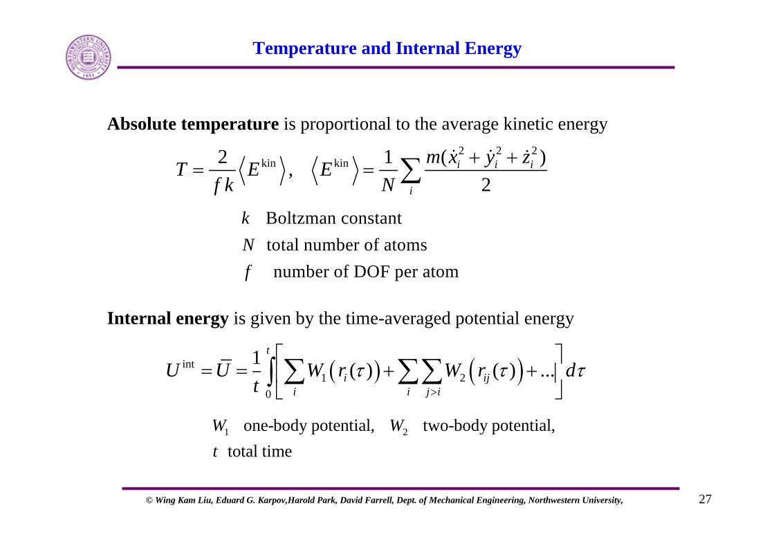
Temperature and Internal Energy

Absolute temperature is proportional to the average kinetic energy

( ) ( )int1 2

0

1 ( ) ( ) ...t

i iji i j i

U U W r W r dt

τ τ τ>

⎡ ⎤= = + +⎢ ⎥

⎣ ⎦∑ ∑∑∫

1 2 one-body potential, two-body potential, total time

W Wt

2 2 2kin kin ( )2 1,

2i i i

i

m x y zT E Ef k N

+ += = ∑

Internal energy is given by the time-averaged potential energy

Boltzman constant total number of atoms number of DOF per atom

kNf


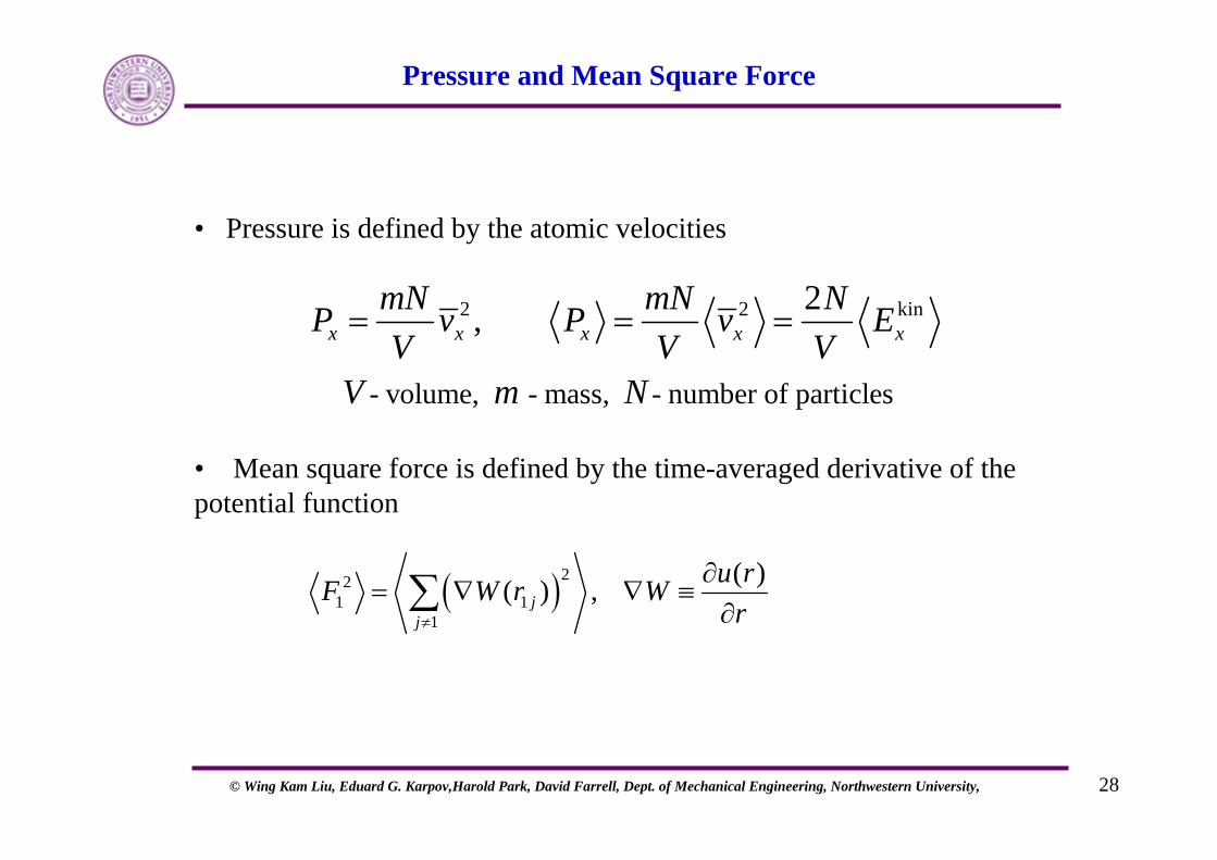
Pressure and Mean Square Force

• Pressure is defined by the atomic velocities

• Mean square force is defined by the time-averaged derivative of the potential function

2 2 kin

- volume, - mass, - number of particles

2,x x x x xmN mN NP v P v EV V V

V m N

= = =

( )221 1

1

( )( ) ,jj

u rF W r Wr≠

∂= ∇ ∇ ≡

∂∑


Entropy

ln Boltzmann constant phase volume integral (over all allowed states)

S kk

= Γ

Γ

( )kin1 13

1 ( ) ( ) ... ...!

0, 0( )

1, 0 Planck's constant

N NN E E U d d d dh N

xx

xh

θ

θ

Γ = − −

<⎧= ⎨ ≥⎩

∫ p r r r p p

For an adiabatically isolated system, the entropy is related to the phase volume integral:

In greater detail, the properties and calculation of entropy for various systems will be discussed on weeks 3-5 lectures.


Thermodynamic Response Functions

The TD response functions reveal how simple thermodynamic quantities respond to changes in measurables, usually either pressure or temperature. Thus, they are derivative quantities (coefficients):

• Heat capacity (how the system internal energy responds to an isometric change in temperature):

• Thermal pressure (how pressure responds to an isometric change in temperature):

• Adiabatic compressibility (how the system volume responds to an isentropic, change in pressure):

vV

ECT∂⎛ ⎞= ⎜ ⎟∂⎝ ⎠

1s

S

VV P

κ ∂⎛ ⎞= − ⎜ ⎟∂⎝ ⎠

vV

PT

γ ∂⎛ ⎞= ⎜ ⎟∂⎝ ⎠


Equilibration

In order to evaluate the averaged macroscopic parameters, the simulated system must achieve a thermodynamic equilibrium. Indeed, the thermodynamic parameters, such as temperature, internal energy, etc., are defined for equilibrium systems.

In the equilibrium:

1) the macroscopic parameters fluctuate around their statistically averaged values;

2) the property averages are stable to small perturbations;

3) different parts of the system yield the same averaged values of the macroscopic parameters.

Equilibration of a macroscopic parameter is achieved in distinct ways in closed adiabaticand isothermal systems (surrounded by a heat bath).

Closed systems: value of the macroscopic parameter fluctuates about the averaged value with a decaying fluctuation amplitude.

Isothermal systems: value of the macroscopic parameter both fluctuates, and also asymptotically approaches the averaged statistical value (examples are to follow).


Adiabatic Example: Interactive Particles in a Circular Chamber

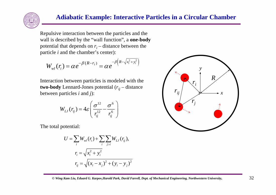
Repulsive interaction between the particles and the wall is described by the “wall function”, a one-bodypotential that depends on ri – distance between the particle i and the chamber’s center):

Interaction between particles is modeled with the two-body Lennard-Jones potential (rij – distance between particles i and j):

The total potential:

12 6

12 6( ) 4LJ ijij ij

W rr rσ σε⎛ ⎞

= −⎜ ⎟⎜ ⎟⎝ ⎠

2 2

2 2

( ) ( ),

( ) ( )

wl i LJ iji i j i

i i i

ij i j i j

U W r W r

r x y

r x x y y

>

= +

= +

= − + −

∑ ∑∑

( )2 2)(( ) i ii

R x y

wl iR rW r e e

ββα α− − +− −= = y

x

riR

rij

rj


Three Particles: Equation of Motion and Solution


Equations of motion:

Parameters:

Initial conditions (nm, m/s):

1 2 3

12 13 23

2 2

2 2

( ) ( ) ( )( ) ( ) ( ),

( ) ( )

wl wl wl

LJ LJ LJ

i i i

ij i j i j

U W r W r W rW r W r W r

r x y

r x x y y

= + ++ + +

= +

= − + −

, , 1, 2,3i i i ii i

U Um x m y ix y

∂ ∂= − = − =

∂ ∂

1 94nm , 10nm, 10 kgR mβ − −= = =

1 1 1 1

2 2 2 2

3 3 3 3

(0) 0, (0) 25, (0) 3.0, (0) 0(0) 0, (0) 30, (0) 0.5, (0) 0(0) 0, (0) 20, (0) 2.5, (0) 0

x x y yx x y yx x y y

= = = − == = = − == = = =


Post-Processing: Energy

Kinetic, potential and total energy vs. time (three particles)

The total energy (solid red line): 9.65x10-25 J. This value does not vary in time

tot kin pot

3kin 2 2

1

pot

( )2 i i

i

E E EmE x y

E U=

= +

= +

≡

∑


Post-Processing: Kinetic Energy, Temperature and Pressure

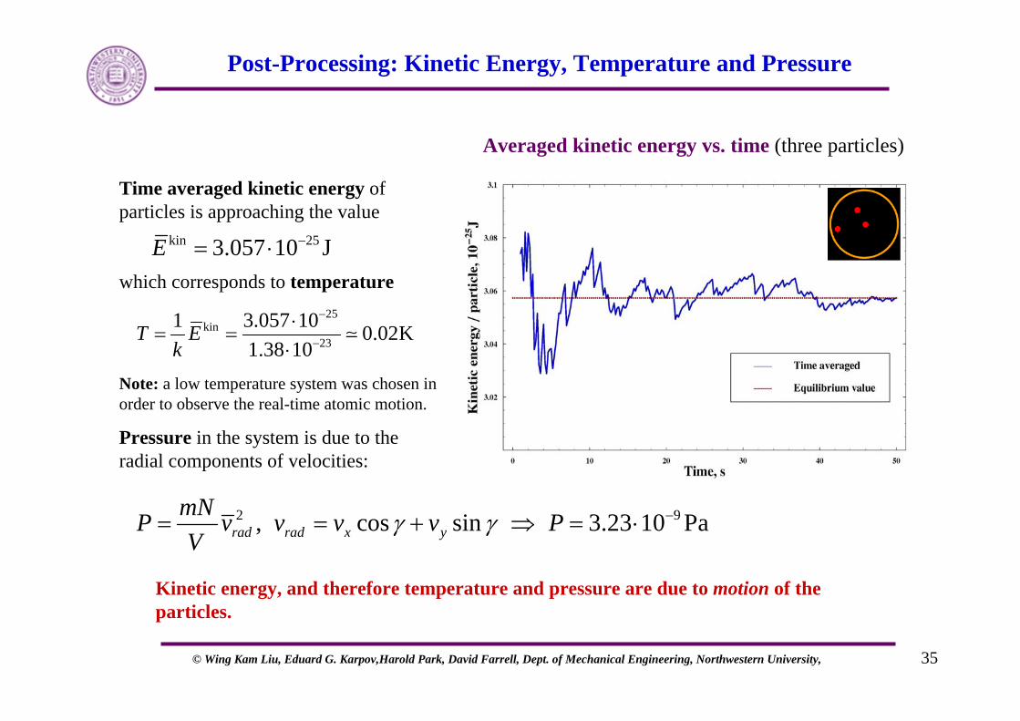
Averaged kinetic energy vs. time (three particles)

Kinetic energy, and therefore temperature and pressure are due to motion of the particles.

Time averaged kinetic energy of particles is approaching the value

which corresponds to temperature

Note: a low temperature system was chosen in order to observe the real-time atomic motion.

Pressure in the system is due to the radial components of velocities:

kin 253.057 10 JE −= ⋅

25kin

23

1 3.057 10 0.02K1.38 10

T Ek

−

−

⋅= =

⋅

2 9, cos sin 3.23 10 Parad rad x ymNP v v v v PV

γ γ −= = + ⇒ = ⋅


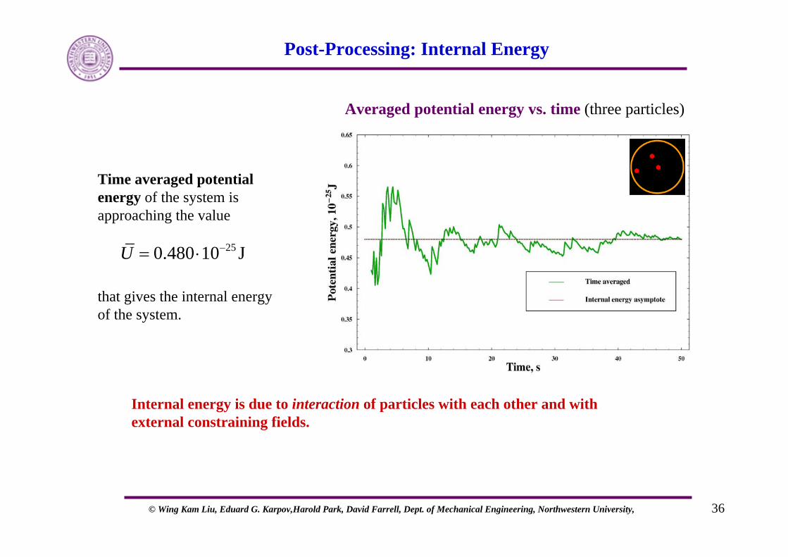
Post-Processing: Internal Energy

Averaged potential energy vs. time (three particles)

Internal energy is due to interaction of particles with each other and with external constraining fields.

Time averaged potential energy of the system is approaching the value

that gives the internal energy of the system.

250.480 10 JU −= ⋅


Five Particles in a Rough Wall: Equations of Motion and Solution



Parameters:

Initial conditions (nm, nm/s):

1 94nm , 10nm, 10 kgR mβ − −= = =

1 1 1 1

2 2 2 2

3 3 3 3

4 4 4 4

5 5 5 5

(0) 0, (0) 25, (0) 5.6, (0) 0(0) 0, (0) 30, (0) 3.0, (0) 0(0) 0, (0) 20, (0) 0.5, (0) 0(0) 0, (0) 24, (0) 2.5, (0) 0(0) 0, (0) 22, (0) 4.9, (0) 0

x x y yx x y yx x y yx x y yx x y y

= = = − == = − = − == = = − == = − = == = = =

wallparticlesLJwallLJ WWWU ++= ∑∑ ,,

The system potential is the sum of the L.J. interactions between the particles, the particles and the wall and a circular wall potential

+ 14 static particles representing the rough wall !

,...3,2,1,, =∂∂

−=∂∂

−= iyUym

xUxm

iii

iii


Five Particles in a Rough Wall: Mathematica Code

Define System Potential, including L.J. Potentials and wall potential, along with simulation parameters

Integrate the equations of motion in time to obtain the trajectories of the particles


Post-Processing: Energy

Kinetic, potential and total energy vs. time (five particles)

The total energy (solid red line): 3.66x10-25 J. This value does not vary in time

UE

yxmE

EEE

poti

iikin

potkintot

≡

+=

+=

∑=

5

1

22 )(2


Post-Processing: Kinetic Energy, Temperature and Pressure

Averaged kinetic energy vs. time (five particles)

Kinetic energy, and therefore temperature and pressure are due to motion of the particles.

Time averaged kinetic energy of particles is approaching the value

which corresponds to temperature

Note: a low temperature system was chosen in order to observe the real-time atomic motion.

JE kin 2510680.2 −⋅=

KEk

T kin 039.01==


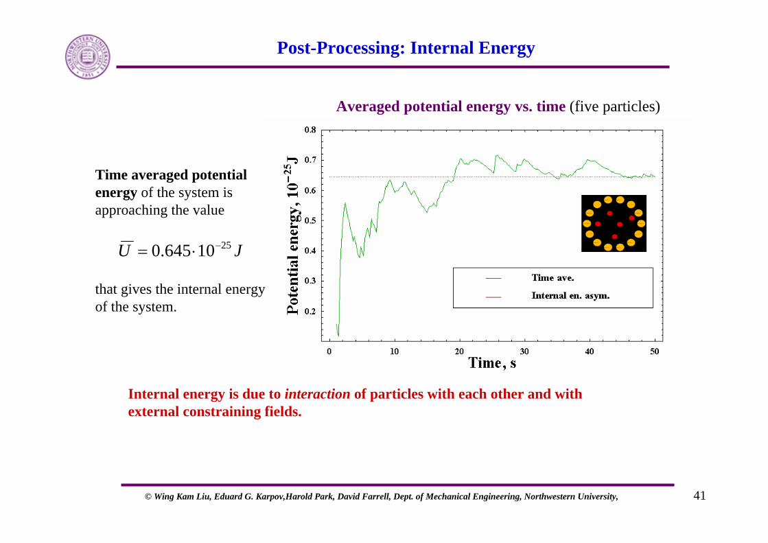
Post-Processing: Internal Energy

Averaged potential energy vs. time (five particles)

Internal energy is due to interaction of particles with each other and with external constraining fields.

Time averaged potential energy of the system is approaching the value

that gives the internal energy of the system.

JU 2510645.0 −⋅=


Limitations of MD

• Realism of forces• Simulation imitates the behavior of a real system only to the extend that

interatomic forces are alike to those that real nuclei would experience when arranged in same configuration

• In simulation forces are obtained as a gradient of a potential energy function, which depends on the positions of the particles

• Realism depends on the ability of potential chosen to replicate the conduct of the material under the circumstance at which the simulation is governed

• Time Limitations• Simulation is “safe” when duration of the simulation is much greater than

relaxation time• Systems have a propensity to become slow and sluggish near phase transitions• Relaxation times order of magnitude larger than times reachable by simulation


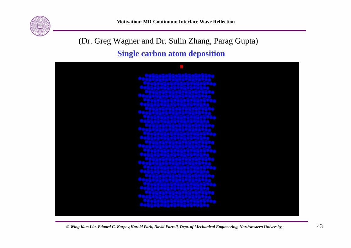
Motivation: MD-Continuum Interface Wave Reflection

Single carbon atom deposition(Dr. Greg Wagner and Dr. Sulin Zhang, Parag Gupta)


Deposition of a Single Atom


Growth of Film: 300 Deposited Atoms

(1,1,1)40eV


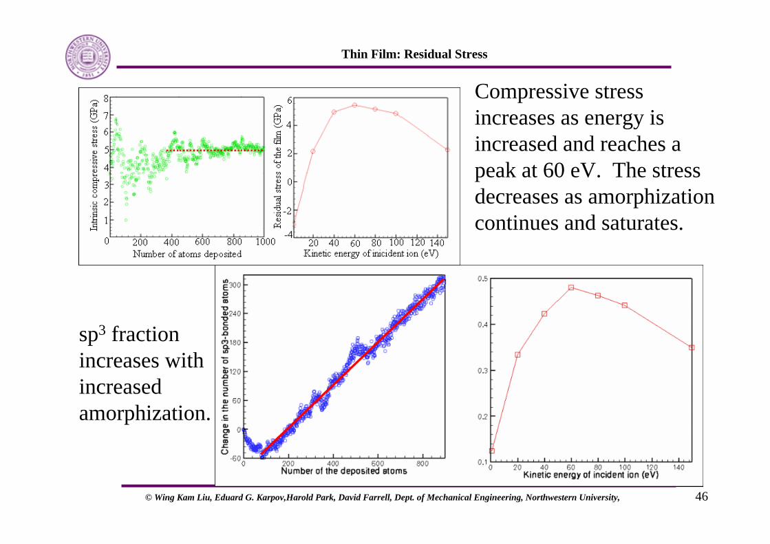
Thin Film: Residual Stress

Compressive stress increases as energy is increased and reaches a peak at 60 eV. The stress decreases as amorphizationcontinues and saturates.

sp3 fraction increases with increased amorphization.


Thin Film: Friction

DLC: Two perfect diamond lattices with sliding in [11-2] exhibit stick-slip motion per period

Amorphous: Deposition added to make hydrogenated amorphous carbon with many asperities on surface and vacancies in lattice


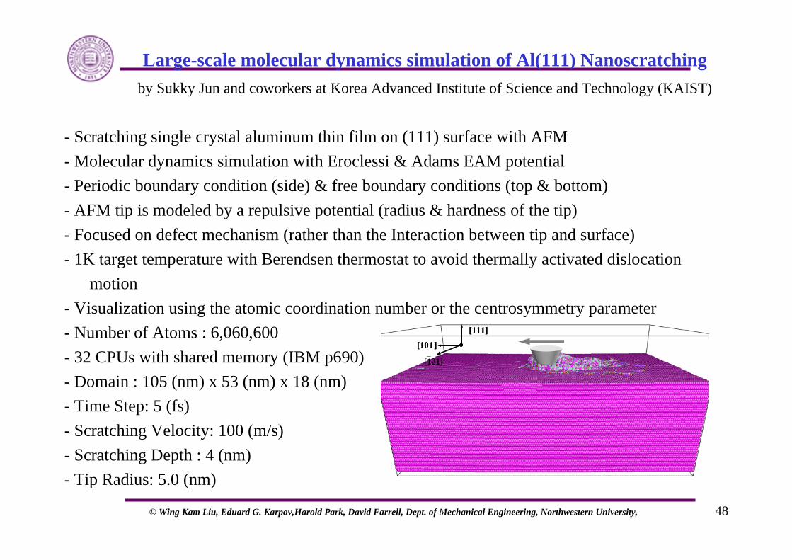
- Scratching single crystal aluminum thin film on (111) surface with AFM- Molecular dynamics simulation with Eroclessi & Adams EAM potential- Periodic boundary condition (side) & free boundary conditions (top & bottom)- AFM tip is modeled by a repulsive potential (radius & hardness of the tip)- Focused on defect mechanism (rather than the Interaction between tip and surface)- 1K target temperature with Berendsen thermostat to avoid thermally activated dislocation

motion- Visualization using the atomic coordination number or the centrosymmetry parameter - Number of Atoms : 6,060,600- 32 CPUs with shared memory (IBM p690)- Domain : 105 (nm) x 53 (nm) x 18 (nm)- Time Step: 5 (fs)- Scratching Velocity: 100 (m/s)- Scratching Depth : 4 (nm)- Tip Radius: 5.0 (nm)

Large-scale molecular dynamics simulation of Al(111) Nanoscratchingby Sukky Jun and coworkers at Korea Advanced Institute of Science and Technology (KAIST)

]1[10

[111]

]1[10

[111]

]1[10

[111]

][ 121


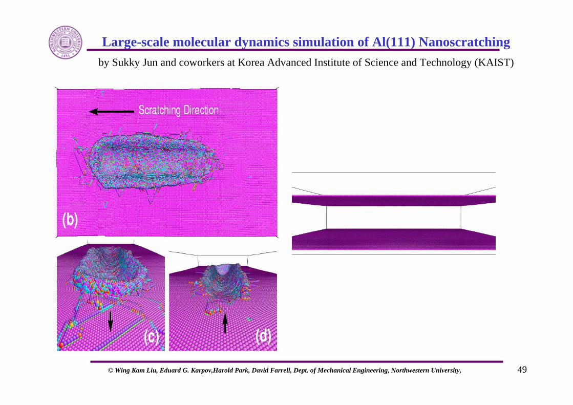
Large-scale molecular dynamics simulation of Al(111) Nanoscratchingby Sukky Jun and coworkers at Korea Advanced Institute of Science and Technology (KAIST)


Some Research Issues –Integration of Nano Science and Engineering

• Unrealistic Assumptions Currently Used for Nano Scale Mechanics and Materials due to Computational Expenses.

– Boundary Conditions for MD are a Major Concern. Need Bridging Scale Techniques.

– Need for the Development of Multiple Scale Mechanics and Materials.


• Self Study Materials


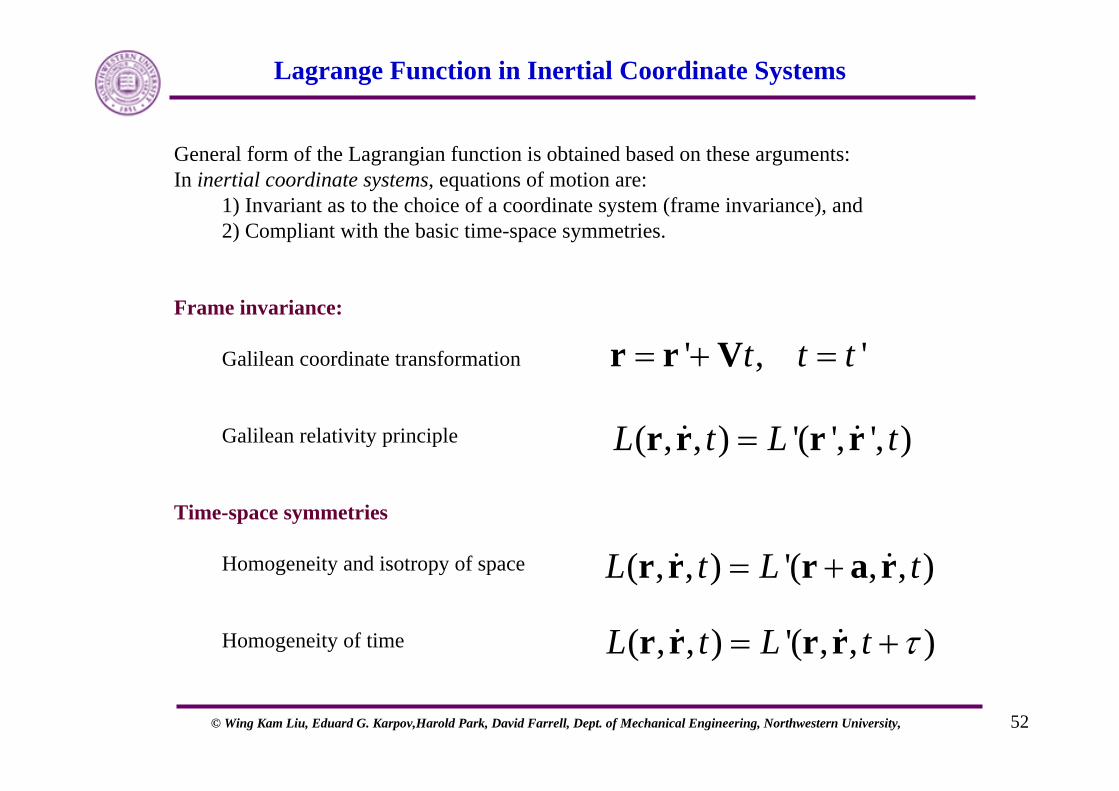
Lagrange Function in Inertial Coordinate Systems

General form of the Lagrangian function is obtained based on these arguments:In inertial coordinate systems, equations of motion are:

1) Invariant as to the choice of a coordinate system (frame invariance), and2) Compliant with the basic time-space symmetries.

Frame invariance:

Galilean coordinate transformation

Galilean relativity principle

Time-space symmetries

Homogeneity and isotropy of space

Homogeneity of time

( , , ) '( ', ', )L t L t=r r r r

' , 't t t= + =r r V

( , , ) '( , , )L t L t= +r r r a r

( , , ) '( , , )L t L t τ= +r r r r


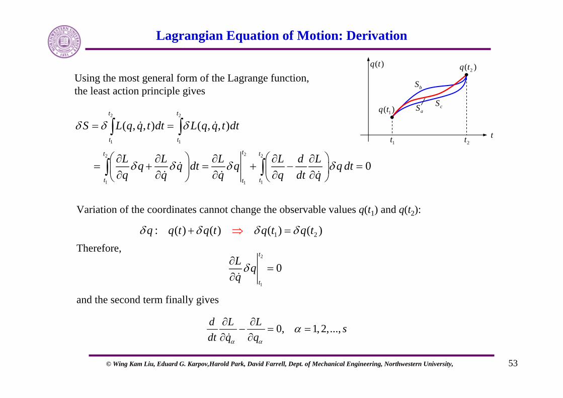
Lagrangian Equation of Motion: Derivation

Using the most general form of the Lagrange function, the least action principle gives

0, 1, 2,...,d L L sdt q qα α

α∂ ∂− = =

∂ ∂

2 2

1 1

22 2

1 11

( , , ) ( , , )

0

t t

t t

tt t

t tt

S L q q t dt L q q t dt

L L L L d Lq q dt q q dtq q q q dt q

δ δ δ

δ δ δ δ

= =

⎛ ⎞ ⎛ ⎞∂ ∂ ∂ ∂ ∂= + = + − =⎜ ⎟ ⎜ ⎟∂ ∂ ∂ ∂ ∂⎝ ⎠ ⎝ ⎠

∫ ∫

∫ ∫

1 2: ( ) ( ) ( ) ( )q q t q t q t q tδ δ δ δ⇒+ =

2( )q t

1( )q t

bS

aS cS

1tt

2t

( )q t

Variation of the coordinates cannot change the observable values q(t1) and q(t2):

Therefore,

and the second term finally gives

2

1

0t

t

L qqδ∂

=∂


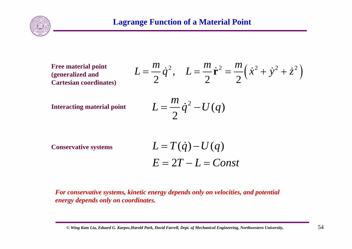
Lagrange Function of a Material Point

Free material point(generalized and Cartesian coordinates)

Interacting material point

Conservative systems

( )2 2 2 2 2,2 2 2m m mL q L x y z= = = + +r

2 ( )2mL q U q= −

( ) ( )2

L T q U qE T L Const= −= − =

For conservative systems, kinetic energy depends only on velocities, and potential energy depends only on coordinates.


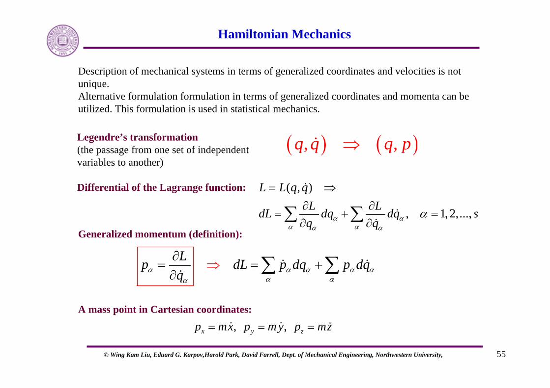
Hamiltonian Mechanics

Description of mechanical systems in terms of generalized coordinates and velocities is not unique.Alternative formulation formulation in terms of generalized coordinates and momenta can be utilized. This formulation is used in statistical mechanics.

( ) ( ), ,q q q p⇒

( , )

, 1, 2,...,

L L q qL LdL dq dq sq qα α

α αα α

α

= ⇒∂ ∂

= + =∂ ∂∑ ∑

Lp dL p dq p dqqα α α α α

α αα

∂= = +∂

⇒ ∑ ∑

Generalized momentum (definition):

A mass point in Cartesian coordinates:

, ,x y zp mx p m y p mz= = =

Legendre’s transformation(the passage from one set of independent variables to another)

Differential of the Lagrange function:


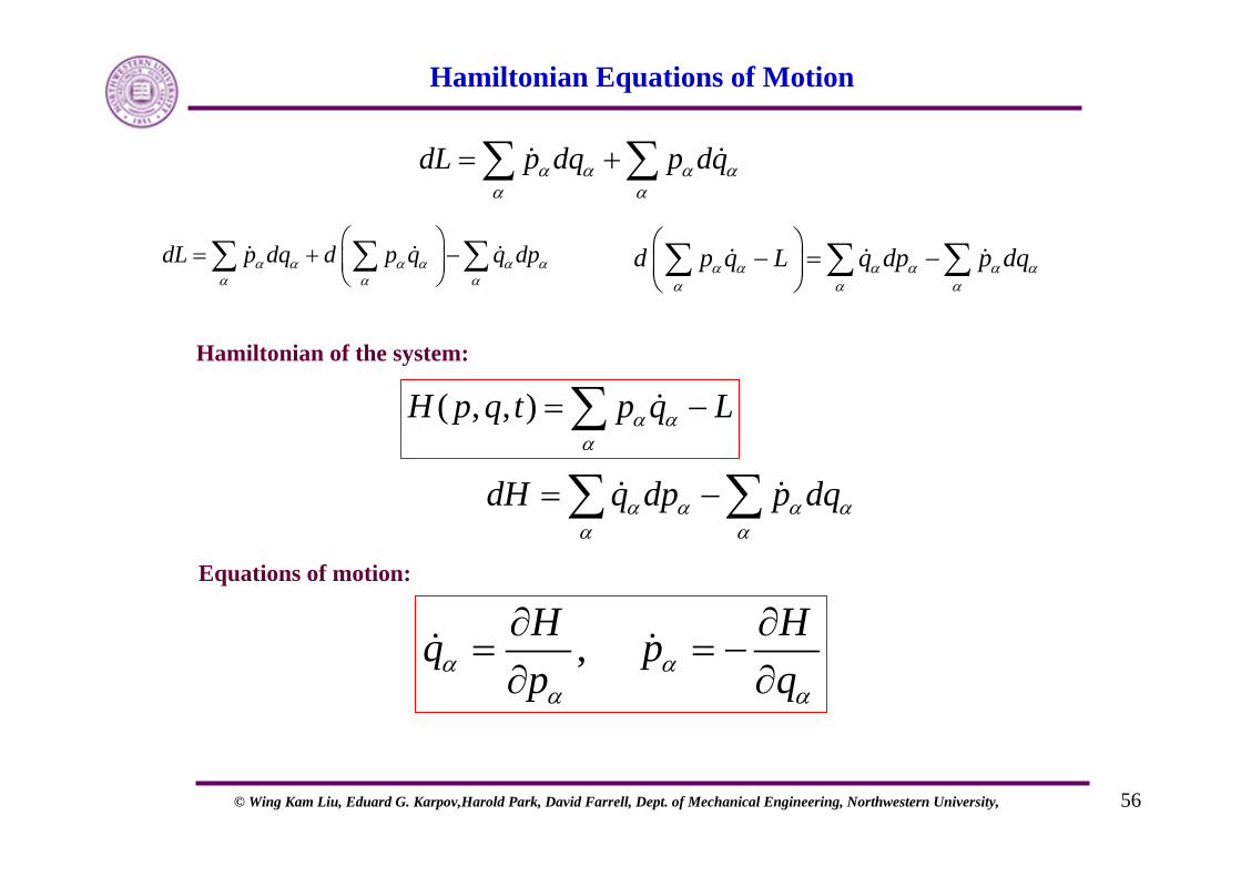
Hamiltonian Equations of Motion

dL p dq p dqα α α αα α

= +∑ ∑

d p q L q dp p dqα α α α α αα α α

⎛ ⎞− = −⎜ ⎟

⎝ ⎠∑ ∑ ∑

Hamiltonian of the system:

dL p dq d p q q dpα α α α α αα α α

⎛ ⎞= + −⎜ ⎟

⎝ ⎠∑ ∑ ∑

( , , )H p q t p q Lα αα

= −∑

dH q dp p dqα α α αα α

= −∑ ∑

,H Hq pp qα αα α

∂ ∂= = −∂ ∂



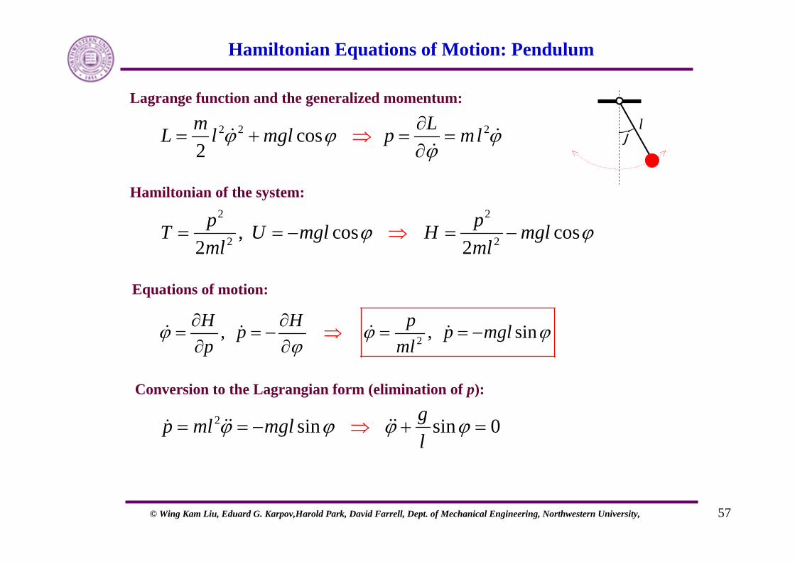
Hamiltonian Equations of Motion: Pendulum


2, , sinH H pp p mglp ml

ϕ ϕ ϕϕ

∂ ∂= = − = = −∂ ∂

⇒


Lagrange function and the generalized momentum:

2 2 2cos2m LL l mgl p mlϕ ϕ ϕ

ϕ∂

= + = =∂

⇒

2 2

2 2, cos cos2 2

p pT U mgl H mglml ml

ϕ ϕ= −⇒= = −

2 sin sin 0gp ml mgll

ϕ ϕ ϕ ϕ= = − =⇒ +

Conversion to the Lagrangian form (elimination of p):

jl


Summary of the Hamiltonian Method

1. The choice of s generalized coordinates (s – number of degrees of freedom).

2. Derivation of the kinetic and potential energy in terms of the generalized coordinates.

3. Derivation of the generalized momenta.

4. Expression of the kinetic energy in terms of the generalized momenta.

5. The sum of the kinetic and potential energies gives the Hamiltonian function.

6. Substitution of the Hamiltonian function into the Lagrangian equation of motion and derivation of a system of 2s first-order differential equations to be solved.

7. Solution of the equations of motion, using a numerical time-integration algorithm.

8. Post-processing and visualization.


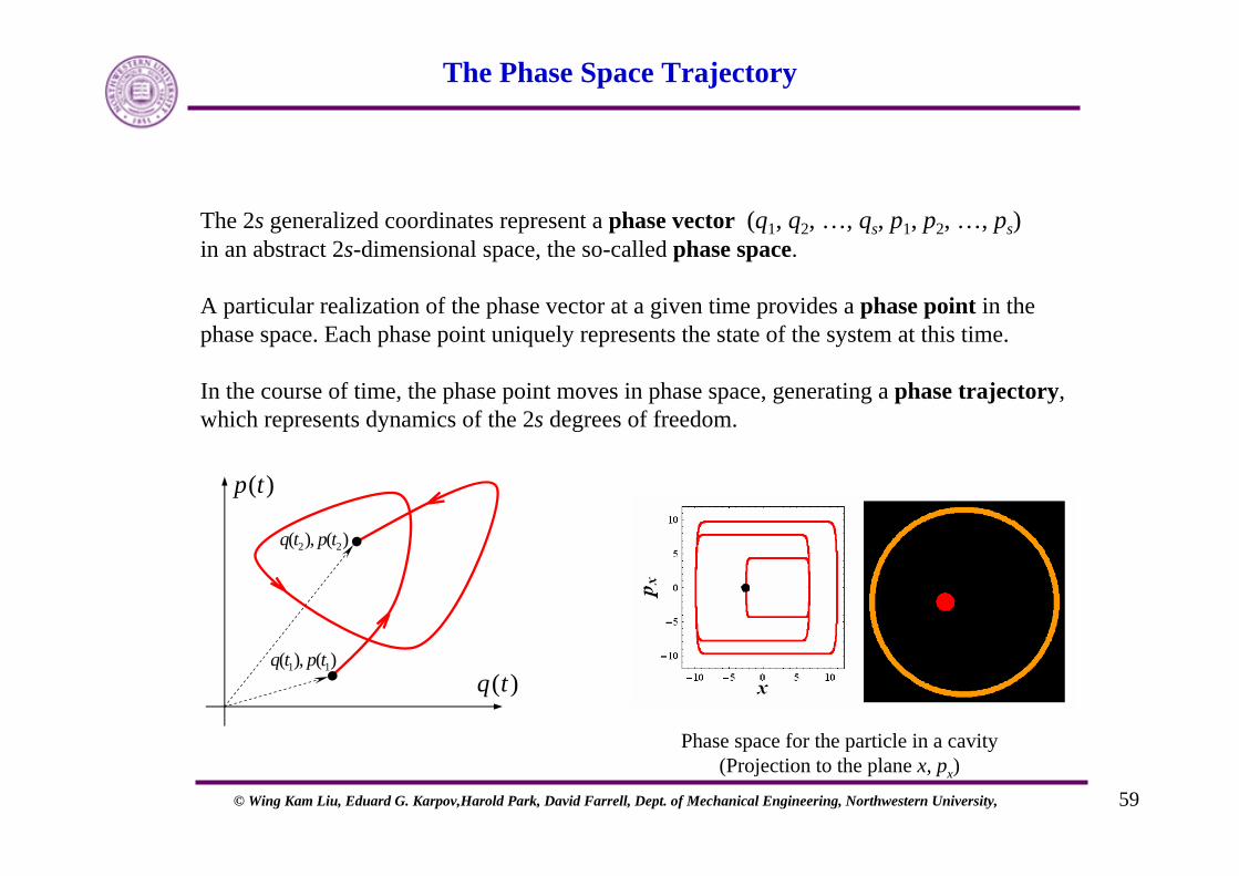
The Phase Space Trajectory

1 1( ), ( )q t p t( )q t

( )p t

2 2( ), ( )q t p t

The 2s generalized coordinates represent a phase vector (q1, q2, …, qs, p1, p2, …, ps)in an abstract 2s-dimensional space, the so-called phase space.

A particular realization of the phase vector at a given time provides a phase point in the phase space. Each phase point uniquely represents the state of the system at this time.

In the course of time, the phase point moves in phase space, generating a phase trajectory, which represents dynamics of the 2s degrees of freedom.

Phase space for the particle in a cavity(Projection to the plane x, px)


Homework Assignment #1a: Generalized Coordinates

Give two examples of mechanical systems, with 2 to 4 degrees of freedom (both distances and angles, or only angles).

Sketch these systems, explaining the available degrees of freedom, and specify the choice of generalized coordinates, as

1 2..., ..., ...q q= =


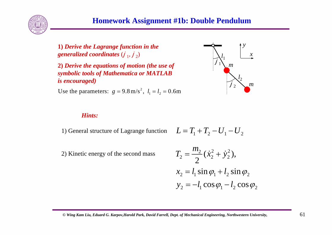
Homework Assignment #1b: Double Pendulum

1 2 1 2L T T U U= + − −

1) Derive the Lagrange function in the generalized coordinates (j1, j2)

2) Derive the equations of motion (the use of symbolic tools of Mathematica or MATLAB is encouraged)

1) General structure of Lagrange function

2) Kinetic energy of the second mass

Hints:

j1l1

l2j2

yx

m

m

2 222 2 2

2 1 1 2 2

2 1 1 2 2

( ),2sin sin

cos cos

mT x y

x l ly l l

ϕ ϕϕ ϕ

= +

= += − −

21 2Use the parameters: 9.8 m/s , 0.6mg l l= = =


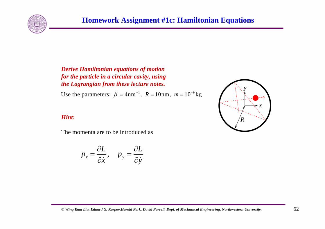
Homework Assignment #1c: Hamiltonian Equations

Derive Hamiltonian equations of motion for the particle in a circular cavity, using the Lagrangian from these lecture notes.

Hint:

The momenta are to be introduced as

,x yL Lp px y∂ ∂

= =∂ ∂

y

x

R

1 9Use the parameters: 4nm , 10nm, 10 kgR mβ − −= = =


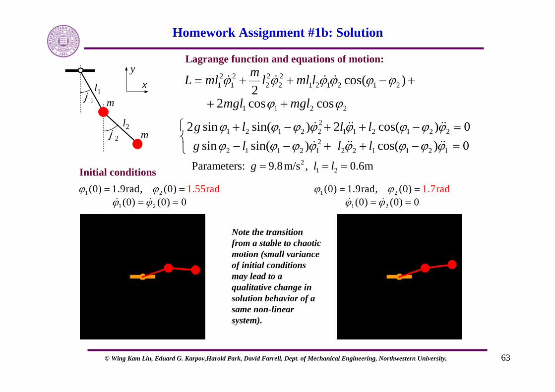
Homework Assignment #1b: Solution

2 2 2 21 1 2 2 1 2 1 2 1 2

1 1 2 2

cos( )2

2 cos cos

mL ml l ml l

mgl mgl

ϕ ϕ ϕ ϕ ϕ ϕ

ϕ ϕ

= + + − +

+ +

Lagrange function and equations of motion:

j1l1

l2j2

yx

m

m2

1 2 1 2 2 1 1 2 1 2 22

2 1 1 2 1 2 2 1 1 2 1

2 sin sin( ) 2 cos( ) 0sin sin( ) cos( ) 0

g l l lg l l l

ϕ ϕ ϕ ϕ ϕ ϕ ϕ ϕϕ ϕ ϕ ϕ ϕ ϕ ϕ ϕ

⎧ + − + + − =⎨

− − + + − =⎩

1 2

1 2

1.55rad(0) 1.9rad, (0)(0) (0) 0

ϕ ϕϕ ϕ

= == =

21 2Parameters: 9.8m/s , 0.6mg l l= = =Initial conditions

1 2

1 2

1.7rad(0) 1.9rad, (0)(0) (0) 0

ϕ ϕϕ ϕ= =

= =

Note the transition from a stable to chaotic motion (small variance of initial conditions may lead to a qualitative change in solution behavior of a same non-linear system).


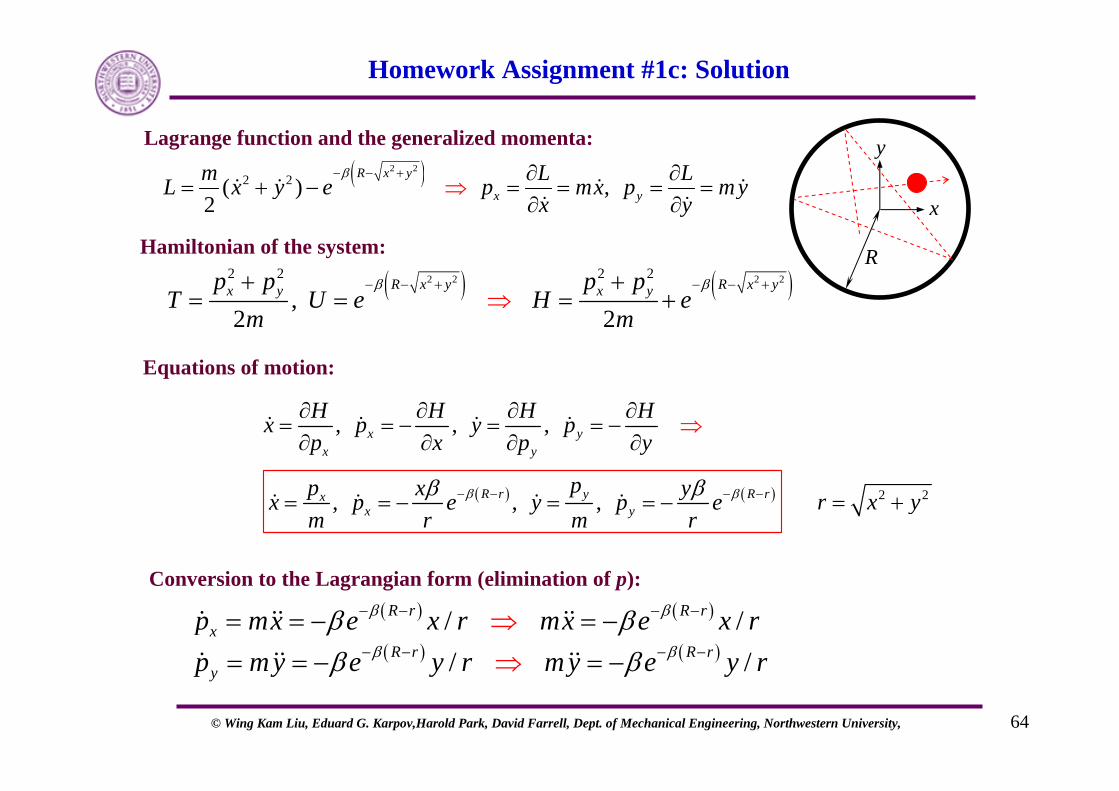
Homework Assignment #1c: Solution


( ) ( )

, , ,

, , ,

x yx y

R r R ryxx y

H H H Hx p y pp x p y

pp x yx p e y p em r m r

β ββ β− − − −

∂ ∂ ∂ ∂= = − = = −∂ ∂ ∂ ∂

= = − = = −

⇒


Lagrange function and the generalized momenta:

( )2 22 2( ) ,

2R x y

x ym L LL x y e p mx p m y

x yβ− − + ∂ ∂

= + − = =⇒ = =∂ ∂

( ) ( )2 2 2 22 2 2 2

,2 2

R x y R x yx y x yp p p pT U e H e

m mβ β− − + − − +

⇒+ +

= = = +

( ) ( )

( ) ( )/ // /

R r R rx

R r R ry

p mx e x r mx e x rp m y e y r m y e y r

β β

β β

β ββ β

− − − −

− − − −

= = − = −= = −

⇒⇒ = −

Conversion to the Lagrangian form (elimination of p):

2 2r x y= +

y

x

R


Truncated Potential

• In system of N atoms

• accumulates unique pair interactions

• if all pair interactions are sampled, the number increases with square of the number of atoms

• Saving computer time

• Neglect pair interactions beyond some distance

• Example: Lennard-Jones potential used in simulations

)1(21

−NN

12 6

4( )

0

cLJ

c

r rW r r r

r r

σ σε⎧ ⎡ ⎤⎛ ⎞ ⎛ ⎞− ≤⎪ ⎢ ⎥⎜ ⎟ ⎜ ⎟= ⎝ ⎠ ⎝ ⎠⎨ ⎢ ⎥⎣ ⎦⎪

>⎩

cr


Instability & Fluctuations in MD Simulations

Macroscopic properties are determined by behavior of individual molecules, in particular:

• Any measurable property can be translated into a function that depends on the positions of phase points in phase space

• The measured value of a property is generated from finite duration experiments

As a phase point travels on a hypersurface of constant energy, most quantities are not constant, but fluctuating (discussed in more detail Week 3 lecture).

While kinetic energy Ek and potential energy U fluctuate, the value of total energy E is preserved,

constkE E U= + =

Due to essential non-linearity of the molecular interaction, classical equations of motion yield non-stable (non-predictable) trajectories.

Therefore, the results of MD simulations are intriguing.


Fluctuations in MD Simulation…

0 2 4 6 8time

1

2

3

4

5

6

elbavresbo

0 2 4 6 8time

1

2

3

4

5

6

degarevaelbavresbo

Averaging of a fluctuating value F(t) over period of time t1 to t2 is accomplished according to

2

12 1

1( ) ( )t

t

F t F t dtt t

=− ∫


Homework Assignment #2a

1) Run the provided Mathematica and MATLAB codes (for 5 particles in a circular chamber and for particles in a rectangular box with periodic boundary conditions, respectively), using a set of arbitrary chosen initial conditions.

2) For 5 particles in the circular chamber: export numerical solution data, compute temperature and internal energy. For the post-processing, modify the Mathematica code provided by updating it from 3 to 5 particles, or write your own post-processing code.

3) Develop a code for 5 particles in a rough wall chamber (formed by 14 static particles). Set up initial velocities, so that initial kinetic energy is the same as in the circular wall example. Compute temperature in the system through the time-averaged kinetic energy (for sufficiently large times, temperatures in the circular and rough wall chambers should be close to each other).

A Visualization Approach to the Principles of Classical ... · Classical Lagrangian/Hamiltonian...

Documents

Transcript of A Visualization Approach to the Principles of Classical ... · Classical Lagrangian/Hamiltonian...