A Univariate Modeling of Total Ozone through Artificial Neural Network and Conventional

Autoregression

Parthasarathi ChakraborthyParthasarathi Chakraborthy1 Goutami ChattopadhyayGoutami Chattopadhyay2

Surajit ChattopadhyaySurajit Chattopadhyay3

1,3 Pailan College of Management and Technology, Pailan College of Management and Technology,KolkataKolkata

2Bengal Engineering and Science University,Bengal Engineering and Science University, ShibpurShibpur

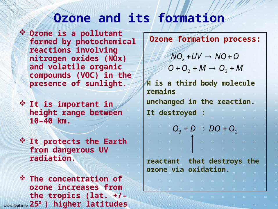
Ozone and its formation Ozone is a pollutant formed by

photochemical reactions involving nitrogen oxides (NOx) and volatile organic compounds (VOC) in the presence of sunlight.

It is important in height range between 10–40 km.

It protects the Earth from dangerous UV radiation.

The concentration of ozone

increases from the tropics (lat. +/- 250 ) higher latitudes in both the hemispheres.

Ozone formation process:

M is a third body molecule remains

unchanged in the reaction.

It destroyed :

reactant that destroys the ozone via oxidation.

ONOUVNO 2

MOMOO 32

23 ODODO

Total Ozone

Total ozone (TO) is a measure of the number of ozone molecules between the ground and the top of the atmosphere, which is the integral of the ozone concentration with respect to height

It is measured in Dobson Unit (DU).

1DU=10-3cm of column ozone at STP

TO comprises both tropospheric and stratospheric ozone. It is responsible for stratospheric heating .

TO is highly variable in nature. The variability is mainly dominated by annual cycle, quasi biennial oscillation (QBO), El Nino Southern Oscillation (ENSO) and solar cycle.

Artificial neural network—an overview

• Artificial Neural Networks (ANN) are biologically inspired networks based on the organization of neurons and decision-making processes in the human brain (Acharya et al. 2003).

• It has been proved by several authors that ANN can be of great use when the associated system is so complex that the underlying processes or relationships are not completely understandable or display chaotic properties.

• Development of an ANN model for any system involves three important issues:

(i) topology of the network,

(ii) a proper training algorithm

(iii) activation function.

• ANN involves an input layer and an output layer connected through one or more hidden layers. The network learns by adjusting the inter connections between the layers.

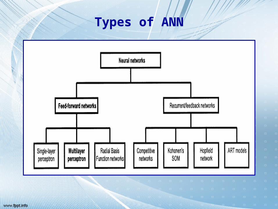
Types of ANN

An overview of MLP• Neural networks, or more precisely artificial neural networks, are a

branch of artificial intelligence. • Multilayer perceptrons (MLP) form one type of neural network• The multilayer perceptron consists of a system of simple

interconnected neurons, or nodes.• The nodes are connected by weights and output signals which are a

function of the sum of the inputs to the node modiÞed by a simple nonlinear transfer, or activation, function.

• It is the superposition of many simple nonlinear transfer functions that enables the multilayer perceptron to approximate extremely non-linear functions.

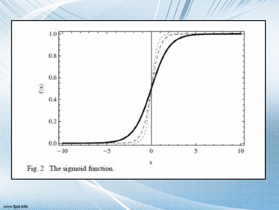
• Due to its easily computed derivative a commonly used transfer function is the sigmoid function

For detailed discussion:M. W. Gardner and S. R. Dorling, 1998, Artificial neural networks (the

multilayer Perceptron)- a review of applications in the Atmospheric sciences, Atmospheric Environment Vol. 32,No. 14/15, pp. 2627-2636

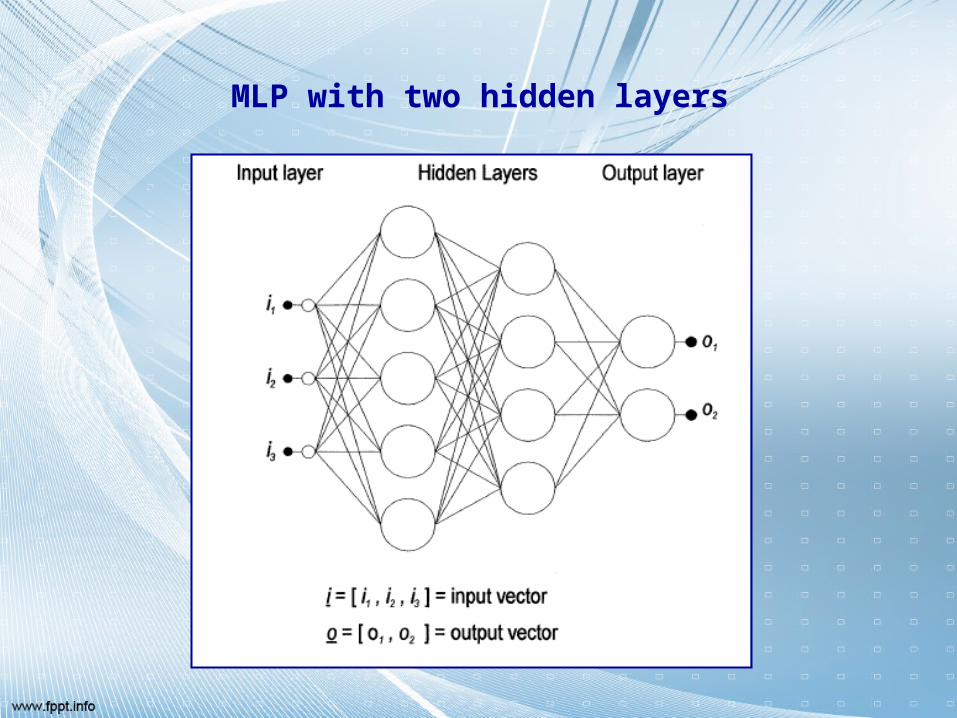
MLP with two hidden layers

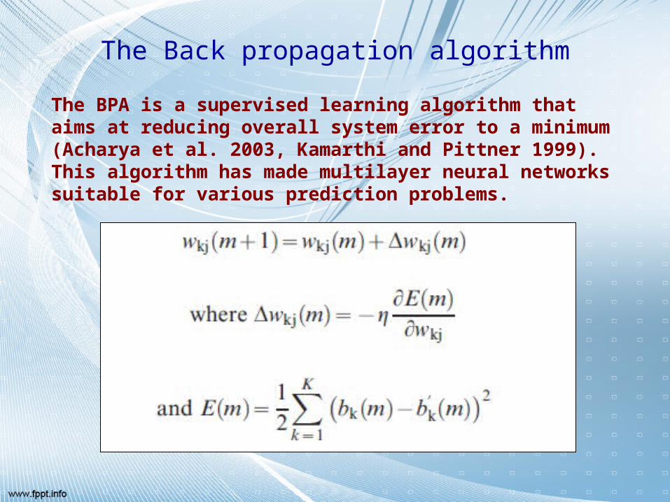
The Back propagation algorithm

The BPA is a supervised learning algorithm that aims at reducing overall system error to a minimum (Acharya et al. 2003, Kamarthi and Pittner 1999). This algorithm has made multilayer neural networks suitable for various prediction problems.

Objectives of the present study• In the present paper, we have considered total ozone The

present study is concerned with the monthly averages of total ozone over Arosa, in Switzerland during the period from 1932 to 1971.

• This study makes an attempt to develop an autoregressive neural network (AR-NN) helpful in predicting the monthly total ozone concentration over Arosa, Switzerland, where the longest time series of total ozone (TO) is available.

• The novelty of the AR-NN proposed lies in using only past data of monthly total ozone concentrations over the study zone and not taking any additional meteorological or environmental predictors.

Advantages of ANN

Advantages of ANN over conventional statistical methods are:

• A priori knowledge of the underlying process is not required.

• Existing complex relationships among the various aspects of the process under investigation need not be recognized.

• Constraints and a priori solution structures are neither assumed nor enforced.

Implementation Procedure

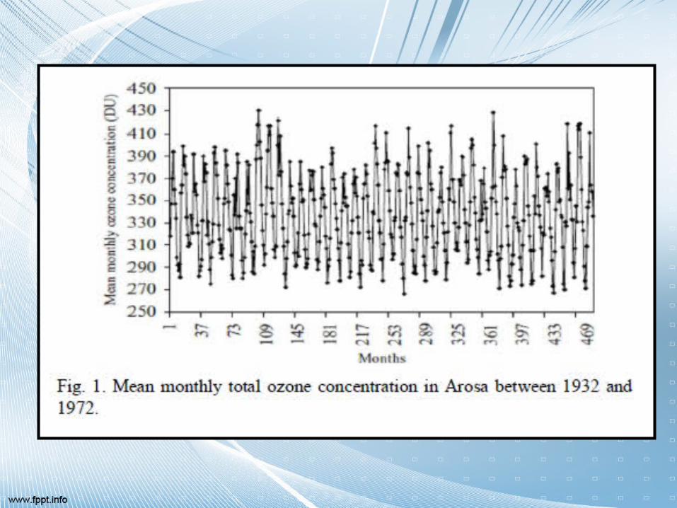
• The present paper deals with mean monthly total ozone concentration in Arosa between 1932 and 1972. The measurements are taken in Dobson Units (DU) (300 DU=1layer of 3 mm if the whole ozone column is taken at sea level with standard conditions). Initially, the raw monthly data are schematically plotted in figure 1. From the data set available from the aforementioned source autocorrelation coefficients (ACC) are computed up to Lag-40.

• It is found that the magnitudes of ACC exhibit local maxima at 6 monthly intervals and are decaying slowly over time. This gives the signal of deterministic components within the time series. From the 6 variables, the first 5 variables are considered as predictor and the 6th variable is considered as the predictand.

• Thus, it is possible to generate a matrix with 487 rows and 6 columns of which the last column indicates the target output. From these 475 rows, first 50% rows are chosen to construct the training set and the remaining 50% rows are chosen to construct the test set or validation set. The activation function for the sequential learning is chosen as the sigmoid function. It should be mentioned that here, the first five variables mean the 5 consecutive values of the total ozone concentration leading up to the sixth observation.

Prediction by AR(5)

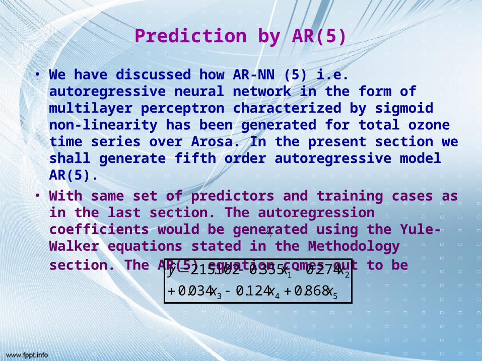
• We have discussed how AR-NN (5) i.e. autoregressive neural network in the form of multilayer perceptron characterized by sigmoid non-linearity has been generated for total ozone time series over Arosa. In the present section we shall generate fifth order autoregressive model AR(5).

• With same set of predictors and training cases as in the last section. The autoregression coefficients would be generated using the Yule-Walker equations stated in the Methodology section. The AR(5) equation comes out to be

j

543

21

868.0124.0034.0

274.0355.0102.215ˆ

xxx

xxy

Skill assessment

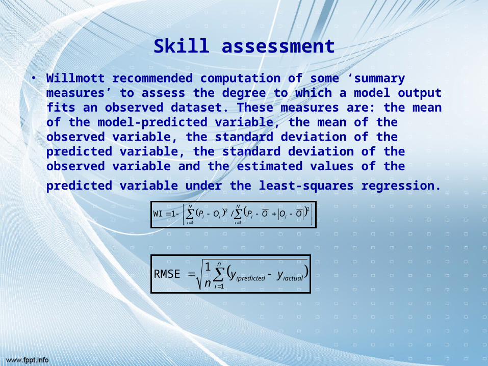
• Willmott recommended computation of some ‘summary measures’ to assess the degree to which a model output fits an observed dataset. These measures are: the mean of the model-predicted variable, the mean of the observed variable, the standard deviation of the predicted variable, the standard deviation of the observed variable and the estimated values of the predicted variable under

the least-squares regression.

N

i

N

iiiii OOOPOP

1 1

22 /1WI

n

iiactualipredicted yy

n 1

1RMSE

• For the two models under consideration we find that for the autoregressive neural network with five predictors we have WI=0.8964 and for the autoregressive model with the same set of predictors WI=0.5617.

• We find that for autoregressive neural network with five predictors RMSE=24.3111 and for conventional autoregression RMSE=75.4635.

Concluding remarks• In this paper we have attempted to model total ozone over Arosa in

univariate manner without using any other meteorological parameters as predictors.

• We find that neurocomputing based model produces higher Willmott’s index and lower root mean squared error than conventional autoregression.

• Therefore, this study demonstrates the superiority of non-linear ANN with backpropagation learning over an autoregressive approach in predicting the mean monthly total ozone concentration in Arosa on the basis of historical values of itself.

• In this model, prediction is possible one month in advance. The study can be extended to examine the influence of future atmospheric parameters.

ReferencesAbdul-Wahab S.A., Bakheit C.S., Al-Alawi S.M., 2005, Principal component

and multiple regression analysis in modelling of ground-level ozone and factors affecting its concentrations, Environmental Modelling and Software, 20 (10), 1263-1271

Acharya, N., Chattopadhyay, S., Kulkarni, M. A., Mohanty, U. C., 2012, A Neurocomputing Approach to Predict Monsoon Rainfall in Monthly Scale Using SST Anomaly as a Predictor, Acta Geophysica, 60, 260-279.

Gardner, M. and Dorling, S., 1998, Artificial neural network (the multilayer per-ceptron) -a review of applications in the atmospheric sciences. Atmospheric Environment, 6, 2627–2636.

Jolliffe I. T., 2002, Principal component analysis. Springer, New York.Sousa, S.I.V., Martins, F.G., Alvim-Ferraz, M.C.M., Pereira, M.C., 2007,

Multiple linear regression and artificial neural networks based on principal components to predict ozone concentrations. Environmental Modelling & Software, 22, 97-103.

Wilks, D. S. 2006, Statistical methods in atmospheric Sciences, Second Edition, Elsevier Inc.

Willmott C. J., 1982, Some Comments on the Evaluation of Model Performance, Bulletin of American Meteorological Society, 63, 1309-1313.