A Unified Perspective on Traffic Flow Theory Part I: The Field - hikari

Applied Mathematical Sciences, Vol. 7, 2013, no. 39, 1929 - 1946HIKARI Ltd, www.m-hikari.com

A Unified Perspective on Traffic Flow Theory

Part I: The Field Theory

Daiheng Ni

Department of Civil and Environmental EngineeringUniversity of Massachusetts, Amherst, MA 01003, USA

[email protected]

Copyright c© 2013 Daiheng Ni. This is an open access article distributed under theCreative Commons Attribution License, which permits unrestricted use, distribution, andreproduction in any medium, provided the original work is properly cited.

Abstract

Over more than half a century, traffic flow theorists have been pur-suing two goals: (1) simple and efficient models to abstract vehiculartraffic flow and (2) a unified framework in which existing traffic flowmodels fit and relate to each other. Continuing these efforts, we reportour humble understanding in a trio of papers. This paper (Part I) intro-duces a Field Theory with an emphasis on traffic flow modeling at themicroscopic level. In this theory, highways and vehicles are perceivedas a field by a driver whose driving strategy is to navigate through thefield along its valley. A special case of the theory, Longitudinal ControlModel, was formulated with specific function form to aid practical ap-plications. Also discussed are properties of the model and its connectionto existing knowledge base.

Keywords: Mathematical modeling, field theory, traffic flow theory

1 Introduction

Three systems are of particular interest: a physical system, a transportationsystem, and a social system, illustrated in Figure 1. The physical system typi-cally consists of non-living objects whose motion and interaction are subject tophysical laws such as Newton’s laws of motion. In contrast, the social systeminvolves living entities such as humans whose behavior vary widely among thepopulation but generally follow some loosely defined rules (e.g. seeking gainsand avoiding losses). As such, physical science is recognized as “hard” since

1930 Daiheng Ni

it is more objective, rigorous, and accurate, while social science is perceivedas “soft” because of its subjectivity, looseness, and inexactness. Straddlingthe above two goes the transportation system which involves both living en-tities (human drivers) and non-living objects (roadways and vehicles). Hence,transportation science can be perceived as “firm” (for the lack of a properword between “hard” and “soft”) since it deals with both physical laws andsocial rules. In addition, it is close to the “soft” end when strategic planningis concerned, while it migrates toward the “hard” end if tactical decision andparticularly operational control are of interest.

Figure 1: Three systems

In this paper, our attention shall be devoted to the modeling of driveroperational control in a transportation system, i.e. the motion and interactionof driver-vehicle units on a long homogeneous highway. By combining physicallaws and social rules, a phenomenology is postulated which represents thedriving environment perceived by a driver as a field. In this field, objects(e.g. roadways and vehicles) are each represented as a component field andtheir union represents the overall hazard that the driver tries to avoid. Hence,the modeling of vehicle motion is simply to seek the least hazardous route bynavigating through the field along its valley.

The paper is arranged as follows. In Section 2, a list of physical phenomenain traffic flow are analyzed in connection with social rules, i.e. the motivationbehind driving decision. The purpose is to demonstrate the similarity be-tween the physical system and the transportation system. As such, a basisis provided that motivates the formulation of the Field Theory in Section 3.Particular attention is drawn to a special case of the Field Theory in Section4 to facilitate the application of the Field Theory. Properties of the specialcase is discussed in Section 5 including its model parameters, ability to de-scribe multiple driving regimes, steady-state behavior under equilibrium, andits connection to existing knowledge base.

A unified perspective on traffic flow theory, part I 1931

2 Physical Basis of Traffic Flow

Many traffic flow phenomena are analogous to those in the physical system,yet the transportation system has something special to distinguish itself.

2.1 Mechanics Phenomena

In Physics, forces are the cause of change of motion. In addition, they aremeasurable and their effects reproducible. For example, Newton’s second lawof motion stipulates that the velocity of an object changes if it is subjectto a non-zero external force; Newton’s third law says that, for every action,there is an equal and opposite reaction. Similarly, “forces” exist in traffic flow,but such forces and subsequently fields are all perceived by the subject driverand hence are subjective matters. As recognized by Lewin (1) and Gibson(2), the distinction between a perceived force and a physical force is that theformer impinges from the inside of the driver through motivation as opposedto through external compulsion. For example, a fast driver feels a “force”(a stress in the driver’s mind) when approaching a slow vehicle. Conversely,the slow driver may or may not be subject to the “reaction force” dependingon whether the driver pays attention and respond to it, i.e., Newton’s thirdlaw may or may not take effect in this case. More examples of mechanicsphenomena are provided below:

M1: Directional flow Traffic always flows in a pre-determined directionmuch like free objects always fall to the ground. The reason why free objectsfall is because they are constantly subject to earth gravity. Similarly, it isreasonable to imagine that vehicles in the traffic are subject to a “gravity”along the roadway. Such a roadway gravity is, again, a subjective matter sinceit exists mentally in drivers and is not measurable, but it is recognized that thegravity is related to factors such as driver personalities (e.g. aggressiveness),vehicle properties (e.g. engine power), and road conditions (e.g. freeways vs.streets).

M2: Free flow An object in free fall will eventually settle on an equilib-rium speed due to air resistance, so does a vehicle in free flow. In this case, the“resistance” comes from the driver’s willingness to comply with traffic rules(e.g. speed limits) as oppose to rolling, grade, and air resistances. Unlike thefree fall speed which is deterministic and replicable given the same condition,the free speed of a vehicle is, once again, a subjective matter because it islargely the driver’s choice. Given the same condition, the choice may varyamong different drivers or at different times. In addition, different roadwayssupport different free speeds. To avoid confusion, the free speed chosen bya driver is called “desired speed”, whereas the free speed aggregated over agroup of vehicles is called “free-flow speed”. Generally, the desired speed is

1932 Daiheng Ni

related to driver personalities and road conditions, while the free flow-speed isaffected by road conditions and driver population.

M3: Stopping at a red light Much like a moving object being stoppedby a wall, a vehicle decelerates to a stop in front of a red light. The “repellingforce” in the latter case resides in the driver and, if he or she ignores thered light, the consequence is costly (e.g. an accident or a ticket). Unlike themoving object which always stops in the same fashion in repeated experiments,drivers are entitled to decelerate at his or her comfortable rate to a stop and,in some extreme cases, drivers may forget to stop.

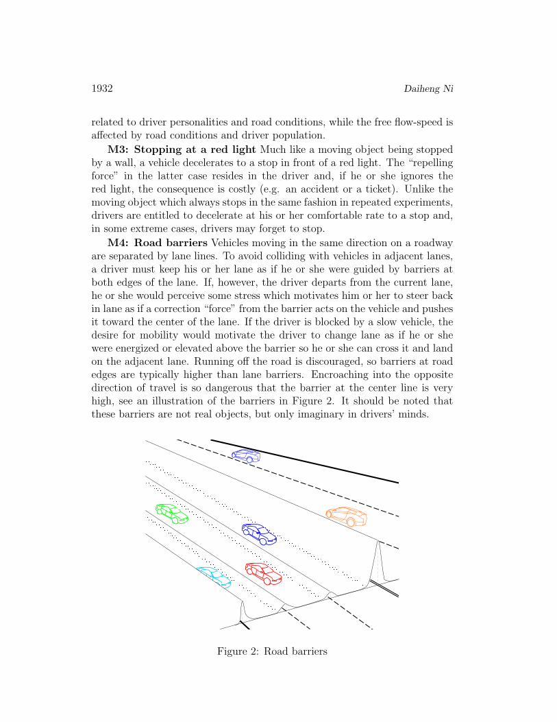
M4: Road barriers Vehicles moving in the same direction on a roadwayare separated by lane lines. To avoid colliding with vehicles in adjacent lanes,a driver must keep his or her lane as if he or she were guided by barriers atboth edges of the lane. If, however, the driver departs from the current lane,he or she would perceive some stress which motivates him or her to steer backin lane as if a correction “force” from the barrier acts on the vehicle and pushesit toward the center of the lane. If the driver is blocked by a slow vehicle, thedesire for mobility would motivate the driver to change lane as if he or shewere energized or elevated above the barrier so he or she can cross it and landon the adjacent lane. Running off the road is discouraged, so barriers at roadedges are typically higher than lane barriers. Encroaching into the oppositedirection of travel is so dangerous that the barrier at the center line is veryhigh, see an illustration of the barriers in Figure 2. It should be noted thatthese barriers are not real objects, but only imaginary in drivers’ minds.

Figure 2: Road barriers


2.2 Electromagnetic Phenomena

An object can exert a force on another object in either of the following twoways: collision and action at a distance. For example, hitting a ball with abat is the former and finding a needle using a magnet is the latter. Thoughcollisions are not uncommon on highways, action at a distance is what vehiclesnormally interact with each other and examples of this kind include some ofthe above mechanics phenomena as well as the following:

E1: Car following Back to the example in the beginning of Section 2where a fast vehicle catches up with a slow vehicle, the fast driver perceivesan imminent collision if he or she keeps driving at that speed. The cost andfear of the collision motivates the fast driver to take actions in advance. If lanechange is not an option and the slow driver does not speed up, the fast driverhas to decelerate and eventually adopts the slow vehicle’s speed separated bya safe following distance. This is analogous to moving a charge A toward alike charge B. According to Coulomb’s law, the electric force between them isdirectly proportional to the product of their charges and inversely proportionalto their distance squared. Similarly, in car following the “force” (stress) actingon the fast driver is larger if he or she approaches the slow vehicle faster andthe distance between them is shorter. However, the same opposite force mayor may not act on the slow driver as he or she may or may not notice thevehicle approaching from behind.

E2: Tailgating Continuing the above example and assuming that the fastvehicle tailgates (i.e. following at a dangerously short distance), it is likelythat the opposite force is perceived by the slow driver who may respond byspeeding up or giving his or her way to the fast follower. Back to the analogy,charge B is now driven (or driven away) by charge A and Newton’s third lawholds in this case. In general, a “force” must be perceived by a driver beforethe force takes effect on the person. In addition, a driver’s ability to perceivedepends on where he or she scans and how frequent this happens.

E3: Shying away If two vehicles happen to run in parallel, one or bothdrivers may feel intimidated. The fear of a side collision motivates them tospread out in space (longitudinally or laterally). Such a shying-away effectbecomes more evident when one of the vehicles is a heavy truck.

2.3 Wave Phenomena

W1: Harmonic wave A platoon of vehicles on a roadway is like a harmonicwave. The platoon is characterized by flow (in vehicles per hour), traffic speed(in km per hour), and density (in vehicles per km), while the wave is deter-mined by frequency (in Hz or cycles per second), wave speed (in meters persecond), and wave length (in meters). One immediately recognizes that flowis equivalent to frequency, traffic speed is equivalent to wave speed, and the

1934 Daiheng Ni

Figure 3: Traffic and waves

spacing (the reciprocal of density) is equivalent to wave length. The upperpart of Figure 3 shows a platoon of vehicles as a harmonic wave.

W2: Signal propagation The signal here does not mean a traffic signal,rather it refers to any quantity that clearly defines the location and speed ofa perturbation in a medium. When the leading vehicle of a compact platoonbrakes briefly, a kinematic wave forms and propagates against the platoon,where the signal here is the brief speed reduction. When a platoon of fastvehicles catch up with a platoon of slow vehicles, a shock wave is generated andpropagates against the traffic, where the signal here is the interface betweenfast and slow vehicles. The bottom part of Figure 3 illustrates a few shockwaves observed in vehicle trajectories.

W3: Wave-particle duality All matter, particularly small-scale objects,exhibits both wave-like and particle-like properties. The latter is prominentwhen individual particles are concerned (e.g. the photoelectric effect), whilethe former becomes significant when the behavior of many particles is viewedcollectively (e.g. diffraction of waves). In traffic flow, individual vehicles actlike particles (e.g. car following and lane changing), while a platoon or platoonsof vehicles exhibit wave property (e.g. kinematic waves and shock waves).

2.4 Statistical Mechanics Phenomena

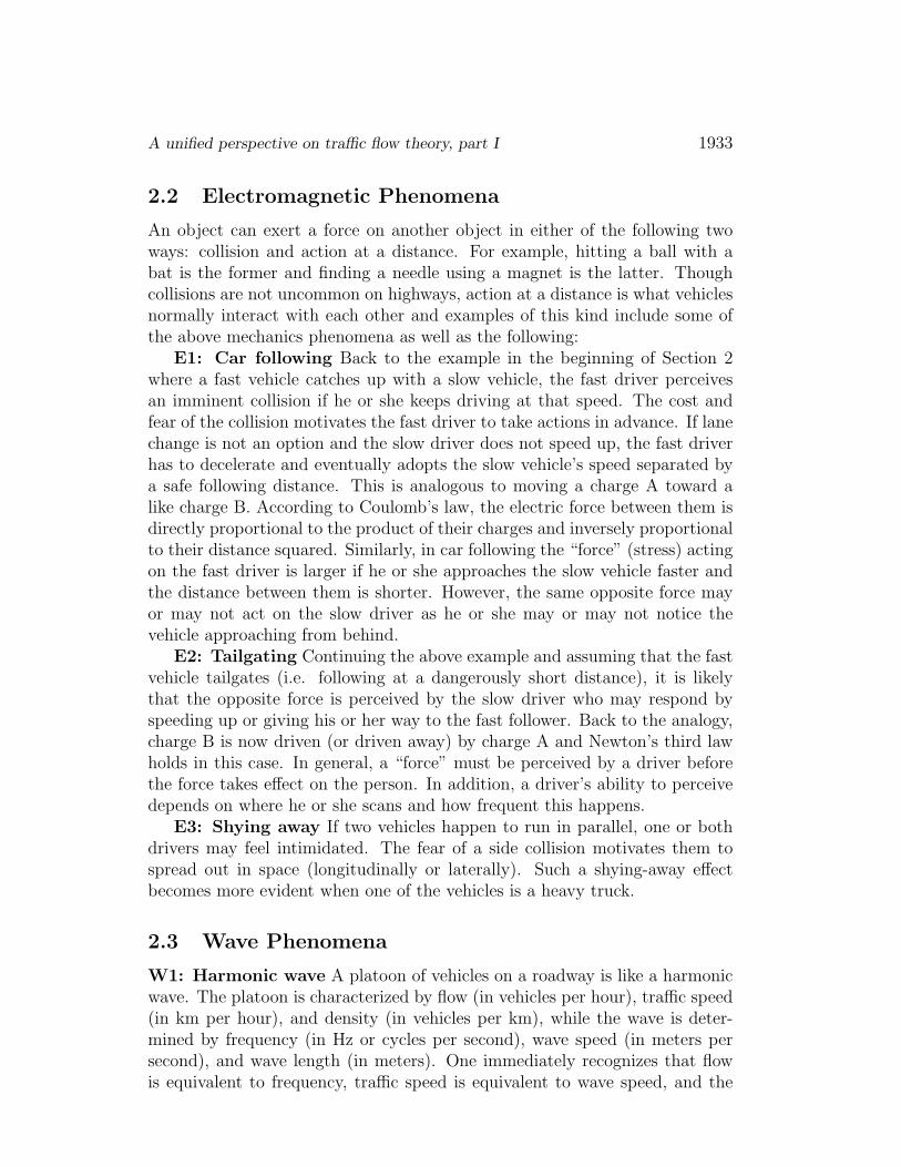
Traffic flow has been modeled by many as a one-dimensional compressible fluid,such as a gas. In gases, the speeds of gas molecules follow Maxwell-Boltzmanndistribution, see an illustration in Part 1 of Figure 4. Remarkable in thedistribution is the increase in average speed and speed variance as temperaturebecomes higher. In contrast, traffic flow exhibits a different trend. Empirical


Molecular speed v, m/s

Num

ber o

f mol

ecul

es

T = 100K

T = 500K T = 1000K

T = 1500K

Spee

d v,

mi/h

Traffic Density k, v/mi

Vehicle speed v, m/s

Num

ber o

f veh

icle

s k = 150 vpm

k = 80 vpm k = 60 vpm

k = 5 vpm

k = 40 vpm

Gas

Traffic Vehicle speed v, mi/h

Prob

abili

ty

5

Traffic density k, v/mi

40 60 80150

Part 1: Maxwell-Boltzmann Distribution Part 2: Empirical speed-density relationship

Part 3: Speed-density distribution Part 4: Stochastic fundamental diagram

Variance not to scale

Figure 4: Maxwell-Boltzmann distribution in traffic flow

observations in Part 2 of the figure show that the variance of traffic speedpeaks around optimal density (where capacity flow occurs) and drops at bothends. Such a distribution is illustrated in Part 3 of the figure in contrast toMaxwell-Boltzmann distribution and further elaborated in a three-dimensionalmodel in Part 4 which forms the basis of a stochastic fundamental diagram.

3 The Field Theory

Lewin (1) defined the “field at a given time” in psychology and Gibson (2)further identified the “field” in automobile driving. However, both offeredtheir discoveries qualitatively without mathematical rigor. Hence, the objec-tive of this section is to formulate the Field Theory of traffic flow. Since thetransportation system involves both living entities (e.g. human drivers) andnon-lining objects (e.g. roadways and vehicles), it is subject to both physicallaws and social rules. As such, the Field Theory is formulated progressivelybased on a set of postulates, two of which (1 and 3) are physical and anothertwo (2 and 4) social.

1936 Daiheng Ni

Postulate 1: A road is a physical field

Postulate 1 is motivated by phenomena M1, M2, and M4 in Section 2. In thelongitudinal (x) direction, a driver-vehicle unit i is subject to a gravity alongthe road:

Gi = migi (1)

where Gi is the roadway gravity acting on the unit, mi is the mass of theunit, and gi is the acceleration of roadway gravity perceived by driver i. Asdiscussed in M1, gi is a function of driver personalities, vehicle properties,and road conditions. Meanwhile, the unit is also subject to a resistance Ri

perceived by the driver due to his or her willingness to observe traffic rules(e.g. speed limits). As discussed in M2, Ri is related to the driver’s perceiveddifference between his or her actual speed xi, and desired speed vi which interm is related to the free-flow speed of the road vf (subscript f here meansfree flow, not a vehicle ID), i.e. Ri = Ri(xi, vi(vf )). Therefore the net forceacting on unit i in the longitudinal direction can be expressed as:

mixi = Gi −Ri (2)

where xi is the acceleration of unit i. Since the right-hand side representsthe amount of net force that can be used to accelerate the unit, it can beinterpreted as the driver’s unsatisfied desire for mobility. As the unit speedsup, the right-hand side decreases because Ri increases. Eventually, the right-hand side varnishes, at which time the unit reaches its desired speed vi. Ifsomehow a random disturbance brings the unit’s speed above vi, the right-hand side becomes negative. In this case, the unit decelerates and finallysettles back to vi.

In the lateral direction of the road, there are lane lines, road edges, andcenter lines to guide and separate traffic. As discussed in M4 of Section 2, thesecross-section elements of the road can be mapped into a roadway potential fieldURi perceived by the driver. When the unit deviates from its lane, the unit

is subject to a correction force Ni which can be interpreted as the stress onthe driver to keep his or her lane, see illustrations in Figures 2 and 6. Theeffect of such a force is to push the unit back to the center of the current lane.Based on physical principles, the force can be determined as the derivative ofthe roadway field, UR

i , with respect to the unit’s lateral displacement yi:

Ni = −∂URi

∂yi(3)


Postulate 2: A driver responds to his surrounding anisotropically

The interaction between two driver-vehicle units differs from the collision oftwo objects in two ways: one pertains to Newton’s third law of motion which isdiscussed below and the other concerns non-contact forces which is the subjectof the next postulate.

In classical physics, Newton’s third law of motion holds when two objectscollide with each other. However, the law generally does not hold in theinteraction between two driver-vehicle units. For example, when a fast vehiclecatches up with a slow vehicle, the fast driver perceives a “repelling force”(i.e. stress) as the gap closes up. The smaller the gap, the greater the force.Conversely, the reaction force may or may not be perceived by the slow driverdepending on whether he or she notices the approaching fast vehicle and hisor her willingness to respond. Since drivers all sit facing front, it is the driverbehind who is responsible for watching safety distances and held liable for arear-end collision should it happen. Therefore, it is not uncommon that aleading driver does not respond to situations happening behind such as anapproaching fast vehicle.

Figure 5: Distribution of driver’s attention

In general, a driver’s responsiveness to his or her surrounding vary withhis or her viewing angle and scanning frequency, see Figure 5. For example,the area right in front of the driver, especially in the same lane, falls into thedriver’s acute vision zone. The driver is responsible for watching this areaconstantly and responding to a situation promptly. Roughly in the driver’sfair vision zones, the frontal areas in side lanes receive considerable amountof the driver’s attention since vehicles in the side lanes may change to thesubject lane and the driver needs to watch these area when making a lanechange. In comparison, the driver scans less frequently at both sides of hisor her vehicle (roughly the driver’s peripheral vision zones) unless the driverneeds to make a lane change or avoid parallel running. The last and leastattended area is the rear of the vehicle not only because it is difficult to access(indirectly by means of side or rear mirrors) but also because the responsibilityrests on drivers behind. Therefore, it is reasonable to assume that the driver’sdirectional response to his or her surrounding, ζi, is a function of his or her

1938 Daiheng Ni

viewing angle αi, i.e.ζi = ζ(αi). Consequently, the force that actually acts onthe unit, Fi, is the product of the force that might have been perceived bythe driver if he or she had paid full attention, Fi, and his or her directionalresponse ζi, i.e.,

Fi = Fi × ζ(αi) (4)

where αi ∈ [−π, π] is the viewing angle. For example, if one chooses ζ(0) = 1and ζ(π) = 0, the driver responds to Fi in full when it comes from the vehiclein front (i.e., αi = 0) and ignores Fi when it comes from the vehicle behind(i.e., αi = π or −π), respectively.

Postulate 3: A driver interacts with others by action at a distance

As described in E1, E2, and E3 in Section 2, a driver is able to sense thepresence of other vehicles and obstacles in its vicinity and take preventiveactions to avoid a collision. It is postulated that such an action at a distanceis mediated by a field which is perceived by the driver as the hazard of collision.One may imagine the field as a hill; the higher and steeper the hill is, the moredifficult it is to climb. The base of the hill/field delineates a region, outside ofwhich the driver is not influenced by the field. For example, the dash-dottedoval (labeled as “Base j”) in Figure 6 represents the base of the field perceivedby driver i due to unit j. One may also interpret the field as the personal spaceof unit j, into which intrusion is discouraged. The deeper unit i intrudes, thestronger repelling force it receives. The longitudinal section of the field isillustrated as the curve above the x axis.

Similarly, unit k represents another field (whose base is labeled as “Basek”) which also exerts an influence on unit i. Since unit k is at the side lane ofunit i, the influence is not in longitudinal x direction but in lateral y direction,i.e., the field results in a repelling force, F k

i , on unit i which motivates it toshy away from unit k.

The above fields and, consequently, forces are related to driver personalitiesand vehicle dynamics. For example, since an aggressive driver accepts shortercar-following distances, the field perceived by such a driver covers a smallerbase. On the other hand, the faster a unit moves, the more hazard it imposeson neighboring vehicles, and thus the larger and steeper the field it creates.

Postulate 4: A driver tries to achieve gains and avoid losses

A driver’s strategy of moving on roadways is to achieve mobility and safety(gains) while avoiding collisions and violation of traffic rules (losses). Such astrategy can be represented using an overall potential field Ui which consists


x

y

i

j

kiF

jiF

iG

xiU ,

yiU ,

),( ii yx

iR

iN

k

Base jBase k

Figure 6: The illustration of a field

of component fields such as those due to moving units UBi , roadways UR

i , andtraffic control devices UC

i , i.e.,

Ui = U(UBi , U

Ri , U

Ci ) (5)

If Ui is viewed as a mountain range whose elevation denotes the risk oflosses, the driver’s strategy is to navigate through the mountain range alongits valley, i.e. the least stressful route. For example, Figure 6 illustrates twosections of such a field. Perceived by driver i, the longitudinal x section of thefield, Ui,x, is dominated by unit j since it is the only neighboring vehicle inthe center lane. Unit i is represented as a ball which rides on the tail of curveUi,x since the vehicle is within unit j’s field. Therefore, unit i is subject to arepelling force F j

i which is derived from Ui,x as:

F ji = −∂Ui,x

∂x(6)

The effect of F ji is to push unit i back to keep safe distance. By incorpo-

rating the driver’s unsatisfied desire for mobility (Gi−Ri), the net force in thex direction can be determined as:

mixi =∑

Fi,x = Gi −Ri − F ji = (migi −Ri) +

∂Ui,x∂x

(7)

The section of Ui in the lateral y direction, Ui,y (the bold curve), is theunion of two components: the cross section of the field due to unit k (the

1940 Daiheng Ni

dashed curve) and that due to the roadway field (the dotted curve). Theformer results in a repelling force F k

i which makes unit i to shy away from unitk and the latter generates a correction force Ni should unit i depart its lanecenter. Therefore, the net effect can be expressed as:

miyi =∑

Fi,y = F ki −Ni = −∂Ui,y

∂y(8)

By incorporating time t, driver i’s perception-reaction time τi, and driveri’s directional response ζi, Equations 7 and 8 can be expressed as:

mixi(t+ τi) =∑

Fi,x(t) = ζ0i [Gi(t)−Ri(t)] + ζ(αji )

∂Ui,x∂x

(9a)

miyi(t+ τi) =∑

Fi,y(t) = −ζ(αki )∂Ui,y∂y

(9b)

where ζ0i ∈ [0, 1] represents the unit’s attention to its unsatisfied desire for

mobility (typically ζ0i = 1), αji and αki are viewing angles which are also func-

tions of time. The above system of equations summarizes the Field Theory ingeneric terms and constitutes the basic law that governs a unit’s motion on aplanar surface.

4 A Special Case

Though the generic form of the Field Theory is able to explain some trafficphenomena qualitatively, rigorous modeling of traffic flow requires a specificform which is the focus of this section. In the generic theory, the functionalforms of the field Ui, roadway gravity Gi, and resistance Ri are undetermined.It appears that the generic theory can take many specific forms and it is im-practical to enumerate all of them. In choosing a specific form, Occam’s razorappears to be a good rule to follow which basically says that “entities shouldnot be multiplied unnecessarily.” Hence, the razor gives rise to the followingconsiderations: (1) the chosen specific form should make physical sense, towhich empirical observations are a good test (this is responded in Part III ofthe paper), (2) it should take a simple functional form (responded in Equation14) that involves physically meaningful parameters but not calibration coeffi-cients (responded in Section 5), and (3) it should provide a sound microscopicbasis for aggregated behavior, i.e. macroscopic equilibrium models (respondedin Section 5 and Part III). With the above considerations, a specific form ofthe theory is formulated by focusing on longitudinal forces which receive fullattention while lateral forces is only considered during a lane change.


4.1 Motion in the Longitudinal Direction

Major forces to be considered are unsatisfied desire for mobility due to roadwaygravity and resistance and action at a distance due to the leading vehicle.

4.1.1 Unsatisfied desire for mobility

The term (Gi−Ri) explains a driver-vehicle unit’s unsatisfied desire for mobil-ity. Intuitively, when a unit starts from stand-still, i.e., xi = 0, its unsatisfieddesire for mobility is the greatest. As the unit speeds up, (Gi −Ri) decreasesaccordingly but is still positive, i.e., it still accelerates the unit to higher speeds.When the unit achieves its desired speed, i.e., xi = vi, its desire for mobilityhas been fully satisfied and, hence, Gi − Ri = 0 which means that the unitsettles at vi if no other forces act on it. If a random perturbation brings xiover vi, the unit’s desire for mobility is over-satisfied and Gi − Ri becomesnegative which decelerates the unit back to vi. With the above understanding,a specific form of the unsatisfied desire for mobility can be formulated as:

Gi −Ri = migi[1− (xivi

)δ] (10)

where δ is a calibration parameter.

4.1.2 Action at a distance

Figure 7: Action at a distance

When a fast unit i (with displacement xi, speed xi, and acceleration xi)catches up a slow unit j (with xj, xj, and xj), the former is subject to anon-contact force, F j

i , from the latter. Such a non-contact force varies withthe spacing between the two units, sij = xj − xi. For example, the forcevirtually has no effect on unit i when it is distant; it takes effect when unit ibecomes close (e.g. within the range of its desired spacing s∗ij); it increases as

1942 Daiheng Ni

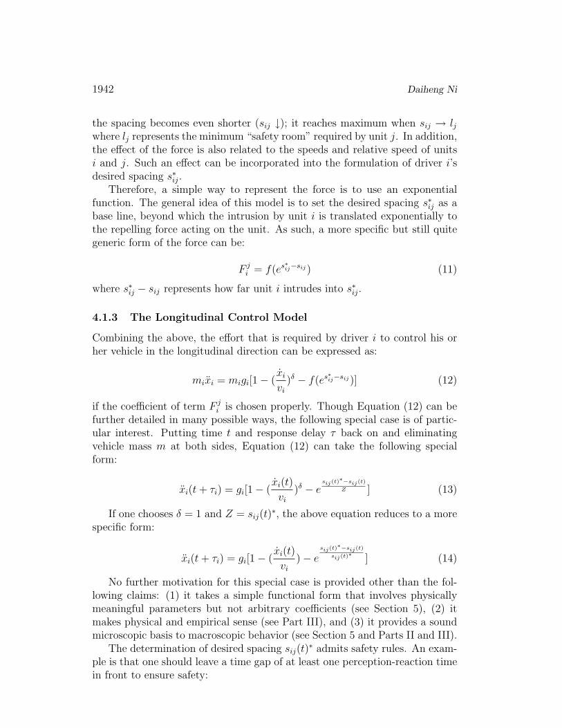
the spacing becomes even shorter (sij ↓); it reaches maximum when sij → ljwhere lj represents the minimum “safety room” required by unit j. In addition,the effect of the force is also related to the speeds and relative speed of unitsi and j. Such an effect can be incorporated into the formulation of driver i’sdesired spacing s∗ij.

Therefore, a simple way to represent the force is to use an exponentialfunction. The general idea of this model is to set the desired spacing s∗ij as abase line, beyond which the intrusion by unit i is translated exponentially tothe repelling force acting on the unit. As such, a more specific but still quitegeneric form of the force can be:

F ji = f(es

∗ij−sij) (11)

where s∗ij − sij represents how far unit i intrudes into s∗ij.

4.1.3 The Longitudinal Control Model

Combining the above, the effort that is required by driver i to control his orher vehicle in the longitudinal direction can be expressed as:

mixi = migi[1− (xivi

)δ − f(es∗ij−sij)] (12)

if the coefficient of term F ji is chosen properly. Though Equation (12) can be

further detailed in many possible ways, the following special case is of partic-ular interest. Putting time t and response delay τ back on and eliminatingvehicle mass m at both sides, Equation (12) can take the following specialform:

xi(t+ τi) = gi[1− (xi(t)

vi)δ − e

sij(t)∗−sij(t)Z ] (13)

If one chooses δ = 1 and Z = sij(t)∗, the above equation reduces to a more

specific form:

xi(t+ τi) = gi[1− (xi(t)

vi)− e

sij(t)∗−sij(t)

sij(t)∗

] (14)

No further motivation for this special case is provided other than the fol-lowing claims: (1) it takes a simple functional form that involves physicallymeaningful parameters but not arbitrary coefficients (see Section 5), (2) itmakes physical and empirical sense (see Part III), and (3) it provides a soundmicroscopic basis to macroscopic behavior (see Section 5 and Parts II and III).

The determination of desired spacing sij(t)∗ admits safety rules. An exam-

ple is that one should leave a time gap of at least one perception-reaction timein front to ensure safety:


s∗ij(t) = xi(t)τi + lj (15)

Another example can be the following: the desired spacing should allowvehicle i to stop behind its leading vehicle j after a perception-reaction timeτi and a deceleration process (at rate bi > 0) should vehicle j applies anemergency brake (at rate Bj > 0). After some math, the desired spacing canbe determined as follows:

s∗ij(t) =x2i (t)

2bi+ xiτi −

x2j(t)

2Bj

+ lj (16)

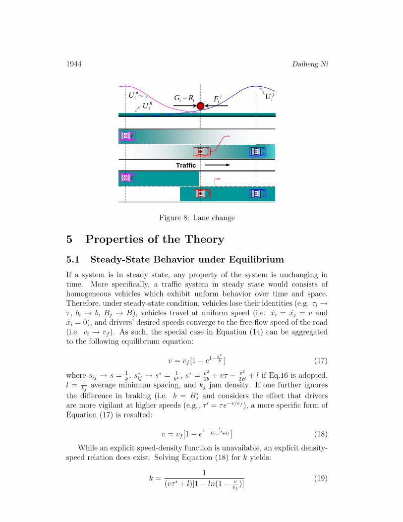
4.2 Motion in the Lateral Direction

A driver-vehicle unit’s motion in the lateral y direction involves decision at twotwo levels: lane change and gap acceptance. A lane change decision concernsthe driver’s desire to change to an adjacent lane to better achieve his or hergoals such as mobility and safety. A gap acceptance decision addresses theexecution of the lane change decision by physically moving the vehicle intothe target lane when an opportunity comes up (e.g. a safe gap is available inthe target lane). Figure 8 illustrates a scenario where units i and j are in theright lane and a trailing neighbor p in the left lane. The top part of the figurepositions unit i (the ball) in its perceived potential fields: U j

i due to unit j inthe same lane, Up

i due to unit p in the left lane, and URi due to road barrier

(lane line). Driven by its desire for mobility, unit i climbs up onto U ji , during

which unit i has to adapt to unit j’s speed while achieving a balance between(Gi−Ri) and F j

i . Under this circumstance, unit i reaches its decision on a lanechange in order to satisfy its desire for mobility. With this decision, driver ibegins to seek opportunities in adjacent lanes. In this example, the right sideis obviously not an option since it is prohibitive to move off-road. Hopefully,an opportunity exists in the left lane because the elevation of unit i (wherethe ball rides) is higher than both lane barrier UR

i and the front of field Upi .

Therefore, unit i initiates a smooth transition by laterally rolling off the tailof U j

i , crossing over URi , and landing onto the front of Up

i , the effect of whichis shown in the middle part of Figure 8.

The above analysis can be simplified by reducing a smooth field to a binary“personal space”. Therefore, a discrete version of lane change is resulted, seethe bottom part of Figure 8.

1944 Daiheng Ni

jiFii RG − j

iU

ji

piU

j

p

Traffic

i

RiU

p

Figure 8: Lane change

5 Properties of the Theory

5.1 Steady-State Behavior under Equilibrium

If a system is in steady state, any property of the system is unchanging intime. More specifically, a traffic system in steady state would consists ofhomogeneous vehicles which exhibit unform behavior over time and space.Therefore, under steady-state condition, vehicles lose their identities (e.g. τi →τ , bi → b, Bj → B), vehicles travel at uniform speed (i.e. xi = xj = v andxi = 0), and drivers’ desired speeds converge to the free-flow speed of the road(i.e. vi → vf ). As such, the special case in Equation (14) can be aggregatedto the following equilibrium equation:

v = vf [1− e1−k∗k ] (17)

where sij → s = 1k, s∗ij → s∗ = 1

k∗, s∗ = v2

2b+ vτ − v2

2B+ l if Eq.16 is adopted,

l = 1kj

average minimum spacing, and kj jam density. If one further ignores

the difference in braking (i.e. b = B) and considers the effect that driversare more vigilant at higher speeds (e.g., τ ′ = τe−v/vf ), a more specific form ofEquation (17) is resulted:

v = vf [1− e1−1

k(vτ ′+l) ] (18)

While an explicit speed-density function is unavailable, an explicit density-speed relation does exist. Solving Equation (18) for k yields:

k =1

(vτ ′ + l)[1− ln(1− vvf

)](19)


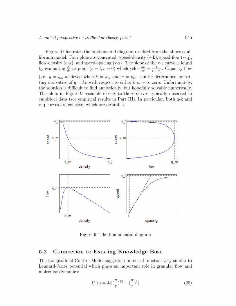
Figure 9 illustrates the fundamental diagram resulted from the above equi-librium model. Four plots are generated: speed-density (v-k), speed-flow (v-q),flow-density (q-k), and speed-spacing (v-s). The slope of the v-s curve is foundby evaluating dv

dsat point (s = l, v = 0) which yelds dv

ds= 1

τ ′+ Lvf

. Capacity flow

(i.e. q = qm achieved when k = km and v = vm) can be determined by set-ting derivative of q = kv with respect to either k or v to zero. Unfortunately,the solution is difficult to find analytically, but hopefully solvable numerically.The plots in Figure 9 resemble closely to those curves typically observed inempirical data (see empirical results in Part III). In particular, both q-k andv-q curves are concave, which are desirable.

Figure 9: The fundamental diagram

5.2 Connection to Existing Knowledge Base

The Longitudinal Control Model suggests a potential function very similar toLennard-Jones potential which plays an important role in granular flow andmolecular dynamics:

U(r) = 4ε[(σ

r)12 − (

σ

r)6] (20)

1946 Daiheng Ni

where U is Lennard-Jones potential due to particle interaction, r is the distancebetween two particles, ε is the depth of the potential well, and σ is the distanceat which the inter-particle potential is zero. The equation is actually a unionof two terms: a long-range attraction term (σ

r)6 (similar to driver’s desire

for mobility) and a short-range repulsion term (σr)12 (similar to inter-vehicle

reaction).Meanwhile, Equation (9) is a special form of Newton’s second law of mo-

tion if one ignores driver’s perception-reaction time τ and directional responseζ. In addition, action at a distance as a means of interaction between driversbecomes a hard collision if driver’s need for safety disappears (i.e. the poten-tial field as a function of spacing U(sij) becomes a spike). Moreover, Newton’sthird law of motion holds if drivers respond to their surroundings isotropically.Furthermore, isotropic response, together with hard collision, gives rise to lawsof momentum and energy conservation. Therefore, the Field Theory representsa special form of classical physics involving human drivers. With its interpre-tation of mean free path (i.e. desired car-following distance s∗ij) and molecularcollision (i.e. action at a distance between vehicles), the Field Theory allowsthe application of other physical principles (such as kinetic theory) to furtherunderstand transportation systems.

ACKNOWLEDGEMENTS. This research is partly sponsored by Uni-versity Transportation Center (UTC) research grants. The author thanks Dr.C. S. Chang, Professor of Civil Engineering at UMass Amherst, for his con-structive comments on the subject matter.

References

[1] Kurt Lewin. Defining the “Field at a Given Time”. Psychological Review,50(3):292–310, 1943.

[2] James J. Gibson and Laurence E. Crooks. A Theoretical Field-Analysis ofAutomobile-Driving. The American Journal of Psychology, 51(3):453–471,1938.Received: November 25, 2012

A Unified Perspective on Traffic Flow Theory Part I: The Field - hikari

Documents

Transcript of A Unified Perspective on Traffic Flow Theory Part I: The Field - hikari