
A Unified View of Performance Metrics: Translating ...
57
Journal of Machine Learning Research 13 (2012) 2813-2869 Submitted 1/12; Revised 7/12; Published 10/12 A Unified View of Performance Metrics: Translating Threshold Choice into Expected Classification Loss Jos´ e Hern´ andez-Orallo JORALLO@DSIC. UPV. ES Departament de Sistemes Inform` atics i Computaci ´ o Universitat Polit` ecnica de Val` encia Cam´ ı de Vera s/n, 46020, Val` encia, Spain Peter Flach PETER.FLACH@BRISTOL. AC. UK Intelligent Systems Laboratory University of Bristol, United Kingdom Merchant Venturers Building, Woodland Road Bristol, BS8 1UB, United Kingdom C` esar Ferri CFERRI @DSIC. UPV. ES Departament de Sistemes Inform` atics i Computaci ´ o Universitat Polit` ecnica de Val` encia Cam´ ı de Vera s/n, 46020, Val` encia, Spain Editor: Charles Elkan Abstract Many performance metrics have been introduced in the literature for the evaluation of classification performance, each of them with different origins and areas of application. These metrics include accuracy, unweighted accuracy, the area under the ROC curve or the ROC convex hull, the mean absolute error and the Brier score or mean squared error (with its decomposition into refinement and calibration). One way of understanding the relations among these metrics is by means of variable operating conditions (in the form of misclassification costs and/or class distributions). Thus, a metric may correspond to some expected loss over different operating conditions. One dimension for the analysis has been the distribution for this range of operating conditions, leading to some important connections in the area of proper scoring rules. We demonstrate in this paper that there is an equally important dimension which has so far received much less attention in the analysis of performance metrics. This dimension is given by the decision rule, which is typically implemented as a threshold choice method when using scoring models. In this paper, we explore many old and new threshold choice methods: fixed, score-uniform, score-driven, rate-driven and optimal, among others. By calculating the expected loss obtained with these threshold choice methods for a uniform range of operating conditions we give clear interpretations of the 0-1 loss, the absolute error, the Brier score, the AUC and the refinement loss respectively. Our analysis provides a comprehensive view of performance metrics as well as a systematic approach to loss minimisation which can be summarised as follows: given a model, apply the threshold choice methods that correspond with the available information about the operating condition, and compare their expected losses. In order to assist in this procedure we also derive several connections between the aforementioned performance metrics, and we highlight the role of calibration in choosing the threshold choice method. Keywords: classification performance metrics, cost-sensitive evaluation, operating condition, Brier score, area under the ROC curve (AUC), calibration loss, refinement loss c 2012 Jos´ e Hern´ andez-Orallo, Peter Flach and C` esar Ferri.
Transcript of A Unified View of Performance Metrics: Translating ...

Journal of Machine Learning Research 13 (2012) 2813-2869 Submitted 1/12; Revised 7/12; Published 10/12
A Unified View of Performance Metrics: Translating ThresholdChoice into Expected Classification Loss
Jose Hernandez-Orallo [email protected]
Departament de Sistemes Informatics i ComputacioUniversitat Politecnica de ValenciaCamı de Vera s/n, 46020, Valencia, Spain
Peter Flach [email protected]
Intelligent Systems LaboratoryUniversity of Bristol, United KingdomMerchant Venturers Building, Woodland RoadBristol, BS8 1UB, United Kingdom
Cesar Ferri [email protected]
Departament de Sistemes Informatics i ComputacioUniversitat Politecnica de ValenciaCamı de Vera s/n, 46020, Valencia, Spain
Editor: Charles Elkan
Abstract
Many performance metrics have been introduced in the literature for the evaluation of classificationperformance, each of them with different origins and areas of application. These metrics includeaccuracy, unweighted accuracy, the area under the ROC curveor the ROC convex hull, the meanabsolute error and the Brier score or mean squared error (with its decomposition into refinement andcalibration). One way of understanding the relations amongthese metrics is by means of variableoperating conditions (in the form of misclassification costs and/or class distributions). Thus, ametric may correspond to some expected loss over different operating conditions. One dimensionfor the analysis has been the distribution for this range of operating conditions, leading to someimportant connections in the area of proper scoring rules. We demonstrate in this paper that thereis an equally important dimension which has so far received much less attention in the analysis ofperformance metrics. This dimension is given by the decision rule, which is typically implementedas athreshold choice methodwhen using scoring models. In this paper, we explore many oldandnew threshold choice methods: fixed, score-uniform, score-driven, rate-driven and optimal, amongothers. By calculating the expected loss obtained with these threshold choice methods for a uniformrange of operating conditions we give clear interpretations of the 0-1 loss, the absolute error, theBrier score, theAUC and the refinement loss respectively. Our analysis providesa comprehensiveview of performance metrics as well as a systematic approachto loss minimisation which can besummarised as follows: given a model, apply the threshold choice methods that correspond withthe available information about the operating condition, and compare their expected losses. Inorder to assist in this procedure we also derive several connections between the aforementionedperformance metrics, and we highlight the role of calibration in choosing the threshold choicemethod.
Keywords: classification performance metrics, cost-sensitive evaluation, operating condition,Brier score, area under the ROC curve (AUC), calibration loss, refinement loss
c©2012 Jose Hernandez-Orallo, Peter Flach and Cesar Ferri.

HERNANDEZ-ORALLO , FLACH AND FERRI
1. Introduction
The choice of a proper performance metric for evaluating classification (Hand, 1997) is an oldbut still lively debate which has incorporated many different performance metrics along the way.Besides accuracy (Acc, or, equivalently, the error rate or 0-1 loss), many other performancemetricshave been studied. The most prominent and well-known metrics are the BrierScore (BS, alsoknown as Mean Squared Error) (Brier, 1950) and its decomposition in terms of refinement andcalibration (Murphy, 1973), the absolute error (MAE), the log(arithmic) loss (or cross-entropy)(Good, 1952) and the area under the ROC curve (AUC, also known as the Wilcoxon-Mann-Whitneystatistic, linearly related to the Gini coefficient and to the Kendall’s tau distanceto a perfect model)(Swets et al., 2000; Fawcett, 2006). There are also many graphical representations and tools formodel evaluation, such as ROC curves (Swets et al., 2000; Fawcett, 2006), ROC isometrics (Flach,2003), cost curves (Drummond and Holte, 2000, 2006), DET curves (Martin et al., 1997), lift charts(Piatetsky-Shapiro and Masand, 1999), and calibration maps (Cohen and Goldszmidt, 2004). Asurvey of graphical methods for classification predictive performanceevaluation can be found inthe work of Prati et al. (2011).
Many classification models can be regarded as functions which output a score for each exampleand class. This score represents a probability estimate of each example to bein one of the classes(or may just represent an unscaled magnitude which is monotonically related with a probabilityestimate). A score can then be converted into a class label using a decision rule. One of the reasonsfor evaluation being so multi-faceted is that models may be learnt in one context(misclassificationcosts, class distribution, etc.) butdeployedin a different context. A context is usually describedby a set of parameters, known asoperating condition. When we have a clear operating conditionat deployment time, there are effective tools such as ROC analysis (Swets et al., 2000; Fawcett,2006) to establish which model is best and what its expected loss will be. However, the question ismore difficult in the general case when we do not have information about the operating conditionwhere the model will be applied. In this case, we want our models to performwell in a widerange of operating conditions. In this context, the notion of ‘proper scoring rule’, see, for example,the work of Murphy and Winkler (1970), sheds some light on some performance metrics. Someproper scoring rules, such as the Brier Score (MSE loss), the logloss,boosting loss and error rate(0-1 loss) have been shown by Buja et al. (2005) to be special cases of an integral over a Betadensity of costs, see, for example, the works of Gneiting and Raftery (2007), Reid and Williamson(2010, 2011) and Brummer (2010). Each performance metric is derived as a special case of the Betadistribution. However, this analysis focusses on scoring rules which are‘proper’, that is, metrics thatare minimised for well-calibrated probability assessments or, in other words, get the best (lowest)score by forecasting the true beliefs. Much less is known (in terms of expected loss for varyingdistributions) about other performance metrics which are non-proper scoring rules, such asAUC.Moreover, even its role as a classification performance metric has been put into question (Hand,2009, 2010; Hand and Anagnostopoulos, 2011).
All these approaches make some (generally implicit and poorly understood)assumptions onhow the model will work for each operating condition. In particular, it is generally assumed that thethreshold which is used to discriminate between the classes will be set according to the operatingcondition. In addition, it is assumed that the threshold will be set in such a waythat the estimatedprobability where the threshold is set is made equal to the operating condition.This is natural ifwe focus on proper scoring rules. Once all this is settled and fixed, different performance metrics
2814

A UNIFIED V IEW OF PERFORMANCEMETRICS
0.48 0.52 0.57 0.62 0.68 0.73 0.78
020
4060
80
Scores
Fre
quen
cy
0.32 0.38 0.43 0.48 0.52 0.57 0.62 0.68 0.73 0.78
020
4060
8010
0
Scores
Fre
quen
cy
Figure 1: Histograms of the score distribution for modelA (left) and modelB (right).
represent different expected losses by using the distribution over the operating condition as a pa-rameter. However, thisthreshold choiceis only one of the many possibilities, as some other workshave explored or mentioned in a more or less explicit way (Wieand et al., 1989; Drummond andHolte, 2006; Hand, 2009, 2010).
In our work we make these assumptions explicit through the concept of athreshold choicemethod,which systematically links performance metrics and expected loss. A thresholdchoicemethod sets a single threshold on the scores of a model in order to arrive atclassifications, possiblytaking circumstances in the deployment context into account, such as the operating condition (theclass or cost distribution) or the intended proportion of positive predictions (the predicted positiverate). Building on this notion of threshold choice method, we are able to systematically explore howknown performance metrics are linked to expected loss, resulting in a rangeof results that are notonly theoretically well-founded but also practically relevant.
The basic insight is the realisation that there are many ways of converting a model (understoodthroughout this paper as a function assigning scores to instances) into a classifier that maps instancesto classes (we assume binary classification throughout). Put differently,there are many ways ofsetting the threshold given a model and an operating condition. We illustrate thiswith an exampleconcerning a very common scenario in machine learning research. Consider two modelsA andB,a naive Bayes model and a decision tree respectively (induced from a training data set), which areevaluated against a test data set, producing a score distribution for the positive and negative classesas shown in Figure 1. We see that scores are in the[0,1] interval and in this example are interpretedas probability estimates for the negative class. ROC curves of both models areshown in Figure2. We will assume that at thisevaluation timewe do not have information about the operatingcondition, but we expect that this information will be available atdeployment time.
If we ask the question of which model is best we may rush to calculate itsAUCandBS(and per-haps other metrics), as given by Table 1. However, we cannot give ananswer because the question isunderspecified. First, we need to know the range of operating conditions the model will workwith.Second, we need to know how we will make the classifications, or in other words, we need adeci-
2815

HERNANDEZ-ORALLO , FLACH AND FERRI
0.0 0.2 0.4 0.6 0.8 1.0
0.0
0.2
0.4
0.6
0.8
1.0
F1
F0
●●●●●●●●●●●●●●●●●●●●●●●●●●●●●●●●●●●●●●●●●●●●●●●●●●●●●●●●●●●●●●●●●●●●●●●●●●●●●●●●●●●●●●●●●●●●●●●●●●●●●●●●●●●●●●●●●●●●●●●●●●●●●●●●●●●●●●●●●●●●●●●
●●●●●●●●●●●●●●●●●●●●●●●
●●●●●●●●●●●●●●●●●●●●
●●●●●●●●●●●●●●●●●●●●●●
●●●●●●●●●●●●●●●●●●●
●●●●●●●●●●●
●●●●●●●●●●●●
●●●●●●●●●●●●●●●●●●●●
●●●●●●●●●●●●●●●●●●●●●●●●●●
●●●●●●●●●●●●●●●●●●●●●
●●●●●●●●●●●●●
●●●●●●●●●●●●●●●●●●●
●●●●●●●●●●●●●●●●●●
●●●●●●●●●●●●●●●●●●●●●●●●●●●●●●●●●
●●●●●●●●●●●●●●●●●●
●●●●●●●●●●●●●●●●●●●●●●●●●●●●●●●●●●●●●●●●●●●●●●
●●●●●●●●●●●●●
●●●●
0.0 0.2 0.4 0.6 0.8 1.0
0.0
0.2
0.4
0.6
0.8
1.0
F1
F0
●
●
●
●
●
●
Figure 2: ROC Curves for modelA (left) and modelB (right).
sion rule, which can be implemented as athreshold choice methodwhen the model outputs scores.For the first dimension (already considered by the work on proper scoring rules), if we have no pre-cise knowledge about the operating condition, we can assume any of many distributions, dependingon whether we have some information about how the cost may be distributed orno information atall. For instance, we can use a symmetric Beta distribution (Hand, 2009), an asymmetric Beta dis-tribution (Hand and Anagnostopoulos, 2011) or, a partial or truncated distribution only consideringa range of costs, or a simple uniform distribution (Drummond and Holte, 2006), as we also do here,which considers all operating conditions equally likely. For the second (new) dimension, wealsohave many options.
performance metric modelA modelBAUC 0.791 0.671
Brier score 0.328 0.231
Table 1: Results from two models on a data set.
For instance, we can just set a fixed threshold at 0.5. This is what naiveBayes and decisiontrees do by default. This decision rule works as follows: if the score is greater than 0.5 then predictnegative (1), otherwise predict positive (0). With this precise decision rule, we can now ask thequestion about the expected misclassification loss for a range of different misclassification costs(and/or class distributions), that is, for a distribution of operating conditions. Assuming a uniformdistribution for operating conditions (cost proportions), we can effectively calculate the answer onthe data set: 0.51.
But we can use other decision rules. We can use decision rules which adapt to the operatingcondition. One of these decision rules is the score-driven threshold choice method, which setsthe threshold equal to the operating condition or, more precisely, to a cost proportionc. Anotherdecision rule is the rate-driven threshold choice method, which sets the threshold in such a way that
2816

A UNIFIED V IEW OF PERFORMANCEMETRICS
the proportion of predicted positives (or predicted positive rate), simply known as ‘rate’ and denotedby r, equals the operating condition. Using these three different threshold choice methods for themodelsA andB, and assuming cost proportions are uniformly distributed, we get the expected lossesshown in Table 2.
threshold choice method expected loss modelA expected loss modelBFixed (T = 0.5) 0.510 0.375
Score-driven (T = c) 0.328 0.231Rate-driven (T s.t. r = c) 0.188 0.248
Table 2: Extension of Table 1 where two models are applied with three different threshold choicemethods each, leading to six different classifiers and corresponding expected losses. In allcases, the expected loss is calculated over a range of cost proportions(operating condi-tions), which is assumed to be uniformly distributed. We denote the threshold byT, thecost proportion byc and the predicted positive rate byr).
In other words, only when we specify or assume a threshold choice methodcan we converta model into a classifier for which it makes sense to consider its expected loss(for a range ordistribution of costs). In fact, as we can see in Table 2, very different expected losses are obtainedfor the same model with different threshold choice methods. And this is the case even assuming thesame uniform cost distribution for all of them.
Once we have made this (new) dimension explicit, we are ready to ask new questions. Howmany threshold choice methods are there? Table 3 shows six of the thresholdchoice methods wewill analyse in this work, along with their notation. Only the score-fixed and thescore-drivenmethods have been analysed in previous works in the area of proper scoring rules. The use ofrates, instead of scores, is assumed inscreeningapplications where an inspection, pre-diagnosis orcoverage rate is intended (Murphy et al., 1987; Wieand et al., 1989), and the idea which underliesthe distinction between rate-uniform and rate-driven is suggested by Hand (2010). In addition, aseventh threshold choice method, known as optimal threshold choice method,denoted byTo, hasbeen (implicitly) used in a few works (Drummond and Holte, 2000, 2006; Hand, 2009).
Threshold choice method Fixed Chosen uniformly Driven by o.c.Using scores score-fixed (Ts f) score-uniform (Tsu) score-driven (Tsd)Using rates rate-fixed (Tr f ) rate-uniform (Tru) rate-driven (Trd)
Table 3: Possible threshold choice methods. The first family uses scores (as they were probabilities)and the second family uses rates (using scores as rank indicators). For both families wecan fix a threshold or assume them ranging uniformly, which makes the threshold choicemethod independent from the operating condition. Only the last column takes the oper-ating condition (o.c.) into account, and hence are the most interesting threshold choicemethods.
2817

HERNANDEZ-ORALLO , FLACH AND FERRI
We will see that each threshold choice method is linked to a specific performance metric. Thismeans that if we decide (or are forced) to use a threshold choice method thenthere is a recom-mended performance metric for it. The results in this paper show that accuracy is the appropriateperformance metric for the score-fixed method,MAE fits the score-uniform method,BS is the ap-propriate performance metric for the score-driven method, andAUC fits both the rate-uniform andthe rate-driven methods. The latter two results assume a uniform cost distribution. It is important tomake this explicit since the uniform cost distribution may be unrealistic in many particular situationsand it is only one of many choices for a reference standard in the general case. As we will mentionat the end of the paper, this suggests that new metrics can be derived by changing this distribution,as Hand (2009) has already done for the optimal threshold choice method with a Beta distribution.
The good news is that inter-comparisons are still possible: given a threshold choice method wecan calculate expected loss from the relevant performance metric. The results in Table 2 allow us toconclude that modelA achieves the lowest expected loss for uniformly sampled cost proportions, ifwe are wise enough to choose the appropriate threshold choice method (in this case the rate-drivenmethod) to turn modelA into a successful classifier. Notice that this cannot be said by just lookingatTable 1 because the metrics in this table are not comparable to each other. In fact, there is no singleperformance metric that ranks the models in the correct order, because,as already said, expectedloss cannot be calculated for models, only for classifiers.
1.1 Contributions and Structure of the Paper
The contributions of this paper to the subject of model evaluation for classification can be sum-marised as follows.
1. The expected loss of a model can only be determined if we select a distribution of operatingconditions and a threshold choice method. We need to set a point in this two-dimensionalspace. Along the second (usually neglected) dimension, several new threshold choice meth-ods are introduced in this paper.
2. We answer the question: “if one is choosing thresholds in a particular way, which perfor-mance metric is appropriate?” by giving an explicit expression for the expected loss for eachthreshold choice method. We derive linear relationships between expectedloss and manycommon performance metrics.
3. Our results reinvigorate AUC as a well-founded measure of expected classification loss forboth the rate-uniform and rate-driven methods. While Hand (2009, 2010) raised objectionsagainst AUC for the optimal threshold choice method only, noting that AUC canbe consis-tent with other threshold choice methods, we encountered a widespread misunderstandingin the machine learning community that the AUC is fundamentally flawed as a performancemetric—a clear misinterpretation of Hand’s papers that we hope that this paper helps to fur-ther rectify.
4. One fundamental and novel result shows that the refinement loss of the convex hull of a ROCcurve is equal to expectedoptimal loss as measured by the area under the optimal cost curve.This sets an optimistic (but also unrealistic) bound for the expected loss.
5. Conversely, from the usual calculation of several well-known performance metrics we canderive expected loss. Thus, classifiers and performance metrics become easily comparable.
2818

A UNIFIED V IEW OF PERFORMANCEMETRICS
With this we do not choose the best model but rather the best classifier (a model with aparticular threshold choice method).
6. By cleverly manipulating scores we can connect several of these performance metrics, eitherby the notion of evenly-spaced scores or perfectly calibrated scores.This provides an addi-tional way of analysing the relation between performance metrics and, of course, thresholdchoice methods.
7. We use all these connections to better understand which threshold choice method should beused, and in which cases some are better than others. The analysis of calibration plays acentral role in this understanding, and also shows that non-proper scoring rules do have theirrole and can lead to lower expected loss than proper scoring rules, whichare, as expected,more appropriate when the model is well-calibrated.
This set of contributions provides an integrated perspective on performance metrics for classifi-cation around the systematic exploration of the notion of threshold choice method that we developin this paper.
The remainder of the paper is structured as follows. Section 2 introduces some notation, thebasic definitions for operating condition, threshold, expected loss, and particularly the notion ofthreshold choice method, which we will use throughout the paper. Section 3 investigates expectedloss for fixed threshold choice methods (score-fixed and rate-fixed),which are the base for the rest.We show that, not surprisingly, the expected loss for these threshold choice method are the 0-1loss (weighted or unweighted accuracy depending on whether we use cost proportions or skews).Section 4 presents the results that the score-uniform threshold choice method hasMAE as associateperformance metric and the score-driven threshold choice method leads tothe Brier score. We alsoshow that one dominates over the other. Section 5 analyses the non-fixed methods based on rates.Somewhat surprisingly, both the rate-uniform threshold choice method andthe rate-driven thresholdchoice method lead to linear functions ofAUC, with the latter always been better than the former.All this vindicates the rate-driven threshold choice method but alsoAUC as a performance metricfor classification. Section 6 uses the optimal threshold choice method, connects the expected lossin this case with the area under the optimal cost curve, and derives its corresponding metric, whichis refinement loss, one of the components of the Brier score decomposition.Section 7 analysesthe connections between the previous threshold choice methods and metrics by considering severalproperties of the scores: evenly-spaced scores and perfectly calibrated scores. This also helps tounderstand which threshold choice method should be used depending on how good scores are.Finally, Section 8 closes the paper with a thorough discussion of results, related work, and an overallconclusion with future work and open questions. Two appendices includea derivation of univariateoperating conditions for costs and skews and some technical results for the optimal threshold choicemethod.
2. Background
In this section we introduce some basic notation and definitions we will need throughout the paper.Further definitions will be introduced when needed. The most important definitions we will needare introduced below: the notion of threshold choice method and the expression of expected loss.
2819

HERNANDEZ-ORALLO , FLACH AND FERRI
2.1 Notation and Basic Definitions
A classifier is a function that maps instancesx from an instance spaceX to classesy from anoutput spaceY. For this paper we will assume binary classifiers, that is,Y = {0,1}. A model is afunctionm: X →R that maps examples to real numbers (scores) on an unspecified scale. Weuse theconvention that higher scores express a stronger belief that the instance is of class 1. Aprobabilisticmodel is a functionm : X → [0,1] that maps examples to estimates ˆp(1|x) of the probability ofexamplex to be of class 1. Throughout the paper we will use the termscore(usually denoted bys)both for unscaled values (in an unbounded interval) and probability estimates (in the interval [0,1]).Nonetheless, we will make the interpretation explicit whenever we use them in one way or the other.We will do similarly for thresholds. In order to make predictions in theY domain, a model can beconverted to a classifier by fixing a decision thresholdt on the scores. Given a predicted scores= m(x), the instancex is classified in class 1 ifs> t, and in class 0 otherwise.
For a given, unspecified model and population from which data are drawn, we denote the scoredensity for classk by fk and the cumulative distribution function byFk. Thus,F0(t) =
∫ t−∞ f0(s)ds=
P(s≤ t|0) is the proportion of class 0 points correctly classified if the decision threshold is t, which isthe sensitivity or true positive rate att. Similarly,F1(t) =
∫ t−∞ f1(s)ds= P(s≤ t|1) is the proportion
of class 1 points incorrectly classified as 0 or the false positive rate at thresholdt; 1−F1(t) is thetrue negative rate or specificity. Note that we use 0 for the positive class and 1 for the negative class,but scores increase with ˆp(1|x). That is,F0(t) andF1(t) are monotonically non-decreasing witht. This has some notational advantages and is the same convention as used by, for example, Hand(2009).
Given a data setD ⊂ 〈X,Y〉 of sizen = |D|, we denote byDk the subset of examples in classk ∈ {0,1}, and setnk = |Dk| and πk = nk/n. Clearly π0 + π1 = 1. We will use the termclassproportion for π0 (other terms such as ‘class ratio’ or ‘class prior’ have been used in the literature).Given a model and a thresholdt, we denote byR(t) the predicted positive rate, that is, the proportionof examples that will be predicted positive (class 0) if the threshold is set att. This can also bedefined asR(t) = π0F0(t)+π1F1(t). The average score of actual classk is sk =
∫ 10 s fk(s)ds. Given
any strict order for a data set ofn examples we will use the indexi on that order to refer to thei-thexample. Thus,si denotes the score of thei-th example andyi its true class.
We define partial class accuracies asAcc0(t) = F0(t) and Acc1(t) = 1− F1(t). From here,(weighted or micro-average) accuracy is defined asAcc(t) = π0Acc0(t)+π1Acc1(t) and (unweight-ed or macro-average) accuracy asuAcc(t) = (Acc0(t)+Acc1(t))/2 (also known as ‘average recall’,Flach, 2012), which computes accuracy while assuming balanced classes.
We denote byUS(x) the continuous uniform distribution of variablex over an intervalS⊂R. Ifthis intervalS is [0,1] thenScan be omitted. The family of continuous distributions Beta is denotedby βα,β. The Beta distributions are always defined in the interval[0,1]. Note that the uniformdistribution is a special case of the Beta family, that is,β1,1 =U .
2.2 Operating Conditions and Expected Loss
When a model is deployed for classification, the conditions might be different to those during train-ing. In fact, a model can be used in several deployment contexts, with different results. A contextcan entail different class distributions, different classification-relatedcosts (either for the attributes,for the class or any other kind of cost), or some other details about the effects that the applicationof a model might entail and the severity of its errors. In practice, a deployment context oroperating
2820

A UNIFIED V IEW OF PERFORMANCEMETRICS
condition is usually defined by a misclassification cost function and a class distribution.Clearly,there is a difference between operating when the cost of misclassifying 0 into 1 is equal to the costof misclassifying 1 into 0 and doing so when the former is ten times the latter. Similarly,operatingwhen classes are balanced is different from when there is an overwhelming majority of instances ofone class.
One general approach to cost-sensitive learning assumes that the costdoes not depend on theexample but only on its class. In this way, misclassification costs are usually simplified by means ofcost matrices, where we can express that some misclassification costs are higher than others (Elkan,2001). Typically, the costs of correct classifications are assumed to be 0. This means that for binarymodels we can describe the cost matrix by two valuesck ≥ 0 with at least one of both being strictlygreater than 0, representing the misclassification cost of an example of classk. Additionally, we cannormalise the costs by settingb= c0+c1, which will be referred to as thecost magnitude(which isclearly strictly greater than 0), andc= c0/b; we will refer toc as thecost proportionSince this canalso be expressed asc= (1+c1/c0)
−1, it is often called ‘cost ratio’ even though, technically, it is aproportion ranging between 0 and 1.
Under these assumptions, an operating condition can be defined as a tupleθ = 〈b,c,π0〉. Thespace of operating conditions is denoted byΘ. These three parameters are not necessarily inde-pendent, as we will discuss in more detail below. The loss for an operating condition is defined asfollows:
Q(t;θ) = Q(t;〈b,c,π0〉), b{cπ0(1−F0(t))+(1−c)π1F1(t)}
= c0π0(1−F0(t))+c1π1F1(t). (1)
It is important to distinguish the information we may have available at each stage of the process. Atevaluation time we may not have access to some information that is available later, at deploymenttime. In many real-world problems, when we have to evaluate or compare models, we do not knowthe operating condition that will apply during deployment. One general approach is to evaluatethe model on a range of possible operating points. In order to do this, we have to set a weight ordistribution for operating conditions.
A key issue when applying a model under different operating conditions ishow the thresholdis chosen in each of them. If we work with a classifier, this question vanishes, since the thresholdis already settled. However, in the general case when we work with a model,we have to decidehow to establish the threshold. The key idea proposed in this paper is the notion of a thresholdchoice method, a function which converts an operating condition into an appropriate threshold forthe classifier.
Definition 1 Threshold choice method. A threshold choice method1 is a (possibly non-determinis-tic) function T: Θ →R such that given an operating condition it returns a decision threshold.
When we say thatT may be non-deterministic, it means that the result may depend on a randomvariable and hence may itself be a random variable according to some distribution. We introduce
1. The notion of threshold choice method could be further generalised to cover situations where we have some informa-tion about the operating condition which cannot be expressed in terms of aspecific value ofΘ, such a distribution onΘ or information aboutE{b}, E{bc}, etc. This generalisation could be explored, but it is not necessary forthe casesdiscussed in this paper.
2821

HERNANDEZ-ORALLO , FLACH AND FERRI
the threshold choice method as an abstract concept since there are several reasonable options forthe functionT, essentially because there may be different degrees of information about the modeland the operating conditions at evaluation time. We can set a fixed threshold ignoring the operatingcondition; we can set the threshold by looking at the ROC curve (or its convex hull) and using thecost proportion to intersect the ROC curve (as ROC analysis does); we can set a threshold looking atthe estimated scores; or we can set a threshold independently from the rank or the scores. The wayin which we set the threshold may dramatically affect performance. But, notless importantly, theperformance metric used for evaluation must be in accordance with the threshold choice method.
Given a threshold choice functionT, the loss for a particular operating conditionθ is givenby Q(T(θ);θ). However, if we do not know the operating condition precisely, we can define adistribution for operating conditions as a multivariate distribution,w(θ). From here, we can nowcalculate expected loss as a weighted average over operating conditions (Adams and Hand, 1999):
L ,
∫Θ
Q(T(θ);θ)w(θ)dθ. (2)
Calculating this integral for a particular case depends on the threshold choice method and thekind of model, but particularly on the space of operating conditionsΘ and its associated distributionw(θ). Typically, the representation of operating conditions is simplified from a three-parameter tuple〈b,c,π0〉 to a single parameter. This reducesw to a univariate distribution. However, this reductionmust carry some assumptions. For instance, the cost magnitudeb is not always independent ofc andπ0, since costs in very imbalanced cases tend to have higher magnitude. For instance, we may havetwo different operating conditions, one withc0 = 10 andc1 = 1 and another withc0 = 5 andc1 = 50.While the cost ratios are symmetric (10:1 withc= 10/11 for the first case, 1:10 withc= 1/11 forthe second), the second operating condition will clearly have more impact onthe expected loss,because its magnitude is five times higher. Moreover,c is usually closely linked toπ0, since thehigher the imbalance (class proportion), the higher the cost proportion. For instance, if positives arerare, we usually want them to be detected (especially in diagnosis and faultdetection applications),and false negatives (i.e., a positive which has not been detected but misclassified as negative) willhave higher cost.
Despite these dependencies, one common option for this simplified operating condition is toconsider that costs are normalised (the cost matrix always sums up to a constant, that is, the costmagnitudeb is constant), or less strongly, thatb andc are independent. Another option which doesnot require independence ofb andc relies on noticing thatb is a multiplicative factor in Equation (1).From here, we just need to assume that the threshold choice method is independent ofb. This is nota strong assumption, since all the threshold choice methods that have been used systematically in theliterature (e.g., the optimal threshold choice method and the score-driven method) are independentof b and so are the rest of methods we work with in this paper. With this, as deployed in appendixA, we can incorporateb in a bivariate distributionvH(〈c,π0〉) for cost and class proportions. Thisdoes not mean that we ignore the magnitudeb or assume it constant, but that we can embed itsvariability in vH . From here, we just derive two univariate cost functions and the correspondingexpected losses.
The first one assumesπ0 constant, leading to a loss expression which only depends on costproportionsc:
Qc(t;c), E{b}{cπ0(1−F0(t))+(1−c)π1F1(t)}. (3)
2822
A UNIFIED V IEW OF PERFORMANCEMETRICS
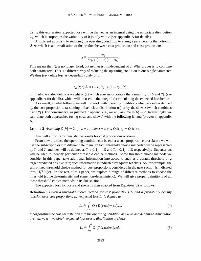
Using this expression, expected loss will be derived as an integral usingthe univariate distributionwc, which incorporates the variability ofb jointly with c (see appendix A for details).
A different approach to reducing the operating condition to a single parameter is the notion ofskew, which is a normalisation of the product between cost proportion and classproportion:
z,cπ0
cπ0+(1−c)(1−π0).
This means thatπ0 is no longer fixed, but neither is it independent ofc. Whatz does is to combineboth parameters. This is a different way of reducing the operating condition to one single parameter.We thus (re-)define loss as depending solely onz.
Qz(t;z), z(1−F0(t))+(1−z)F1(t).
Similarly, we also define a weightwz(z) which also incorporates the variability ofb andπ0 (seeappendix A for details), which will be used in the integral for calculating the expected loss below.
As a result, in what follows, we will just work with operating conditions which are either definedby the cost proportionc (assuming a fixed class distributionπ0) or by the skewz (which combinesc andπ0). For convenience, as justified in appendix A, we will assumeE{b}= 2. Interestingly, wecan relate both approaches (using costs and skews) with the following lemma (proven in appendixA):
Lemma 2 AssumingE{b}= 2, if π0 = π1 then z= c and Qz(t;z) = Qc(t;c).
This will allow us to translate the results for cost proportions to skews.From now on, since the operating condition can be either a cost proportionc or a skewzwe will
use the subscriptc or z to differentiate them. In fact, threshold choice methods will be representedby Tc andTz and they will be defined asTc : [0,1]→R andTz : [0,1]→R respectively. Superscriptswill be used to identify particular threshold choice methods. Some threshold choice methods weconsider in this paper take additional information into account, such as a default threshold or atarget predicted positive rate; such information is indicated by square brackets. So, for example, thescore-fixed threshold choice method for cost proportions consideredin the next section is indicatedthus: Ts f
c [t](c). In the rest of this paper, we explore a range of different methods to choose thethreshold (some deterministic and some non-deterministic). We will give properdefinitions of allthese threshold choice methods in its due section.
The expected loss for costs and skews is then adapted from Equation (2)as follows:
Definition 3 Given a threshold choice method for cost proportions Tc and a probability densityfunction over cost proportions wc, expected lossLc is defined as
Lc ,
∫ 1
0Qc(Tc(c);c)wc(c)dc. (4)
Incorporating the class distribution into the operating condition as skews anddefining a distributionover skews wz, we obtain expected loss over a distribution of skews:
Lz ,
∫ 1
0Qz(Tz(z);z)wz(z)dz. (5)
2823

HERNANDEZ-ORALLO , FLACH AND FERRI
It is worth noting that if we plotQc or Qz againstc andz, respectively, we obtaincost curvesasdefined by Drummond and Holte (2000, 2006). Cost curves are also known as risk curves (e.g.,Reid and Williamson, 2011, where the plot can also be shown in terms ofpriors, that is, classproportions).
Equations (4) and (5) illustrate the space we explore in this paper. Two parameters determinethe expected loss:wc(c) andTc(c) (respectivelywz(z) andTz(z)). While much work has been doneon a first dimension, by changingwc(c) or wz(z), particularly in the area of proper scoring rules,no work hassystematicallyanalysed what happens when changing the second dimension,Tc(c) orTz(z).
This means that in this paper we focus on this second dimension, and just makesome simplechoices for the first dimension. Except for cases where the threshold choice is independent of theoperating condition, we will assume a uniform distribution forwc(c) andwz(z). This is of coursejust one possible choice, but not an arbitrary choice for a number of reasons:
• The uniform distribution is arguably the simplest distribution for a value between 0 and 1 andrequires no parameters.
• This distribution makes the representation of the loss straightforward, sincewe can plotQ onthey-axis versusc (or z) on thex-axis, where thex-axis can be shown linearly from 0 to 1,without any distribution warping. This makes metrics correspond exactly with the areas undermany cost curves, such as the optimal cost curves (Drummond and Holte, 2006), the Briercurves (Hernandez-Orallo et al., 2011) or the rate-driven/Kendall curves (Hernandez-Oralloet al., 2012).
• The uniform distribution is a reasonable choice if we want a model to behavewell in a widerange of situations, from high costs for false positives to the other extreme. In this sense,it gives more relevance to models which perform well when the cost matricesor the classproportions are highly imbalanced.
• Most of the connections with the existing metrics are obtained with this distribution and notwith others, which is informative about what the metrics implicitly assume (if understood asmeasures of expected loss).
Many expressions in this paper can be fine-tuned with other distributions, such as the Beta distri-butionβ(2,2), as suggested by Hand (2009), or using imbalance (Hand, 2010). However, it is theuniform distribution which leads us to many well-known evaluation metrics.
3. Expected Loss for Fixed-Threshold Classifiers
The easiest way to choose the threshold is to set it to a pre-defined valuetfixed, independently fromthe model and also from the operating condition. This is, in fact, what many classifiers do (e.g.,Naive Bayes choosestfixed = 0.5 independently from the model and independently from the operat-ing condition). We will see the straightforward result that this threshold choice method correspondsto 0-1 loss. Part of these results will be useful to better understand some other threshold choicemethods.
Definition 4 Thescore-fixed threshold choice methodis defined as follows:
Ts fc [t](c), Ts f
z [t](z), t. (6)
2824

A UNIFIED V IEW OF PERFORMANCEMETRICS
This choice has been criticised in two ways, but is still frequently used. Firstly, choosing 0.5as a threshold is not generally the best choice even for balanced data sets or for applications wherethe test distribution is equal to the training distribution (see, for example, the work of Lachiche andFlach, 2003 on how to get much more from a Bayes classifier by simply changing the threshold).Secondly, even if we are able to find a better value than 0.5, this does not mean that this value is bestfor every skew or cost proportion—this is precisely one of the reasonswhy ROC analysis is used(Provost and Fawcett, 2001). Only when we know the deployment operating condition at evaluationtime is it reasonable to fix the threshold according to this information. So either bycommon choiceor because we have this latter case, consider then that we are going to usethe same thresholdtindependently of skews or cost proportions. Given this threshold choice method, then the questionis: if we must evaluate a model before application for a wide range of skews and cost proportions,which performance metric should be used?This is what we answer below.
If we plug Ts fc (Equation 6) into the general formula of the expected loss for a range of cost
proportions (Equation 4) we have:
Ls fc (t),
∫ 1
0Qc(T
s fc [t](c);c)wc(c)dc.
We obtain the following straightforward result.
Theorem 5 If a classifier sets the decision threshold at a fixed value t irrespective ofthe operatingcondition or the model, then expected loss for any cost distribution wc is given by:
Ls fc (t) = 2Ewc{c}(1−Acc(t))+4π1F1(t)
(
12−Ewc{c}
)
.
Proof
Ls fc (t) =
∫ 1
0Qc(T
s fc [t](c);c)wc(c)dc=
∫ 1
0Qc(t;c)wc(c)dc
=∫ 1
02{cπ0(1−F0(t))+(1−c)π1F1(t)}wc(c)dc
= 2π0(1−F0(t))∫ 1
0cwc(c)dc+2π1F1(t)
∫ 1
0(1−c)wc(c)dc
= 2π0(1−F0(t))Ewc{c}+2π1F1(t)(1−Ewc{c})
= 2π0(1−F0(t))Ewc{c}+2π1F1(t)
(
Ewc{c}+2
(
12−Ewc{c}
))
= 2Ewc{c}(π0(1−F0(t))+π1F1(t))+4π1F1(t)
(
12−Ewc{c}
)
= 2Ewc{c}(1−Acc(t))+4π1F1(t)
(
12−Ewc{c}
)
.
2825

HERNANDEZ-ORALLO , FLACH AND FERRI
This gives an expression of expected loss which depends on error rate and false positive rate att and the expected value for the distribution of costs.2 Similarly, if we plugTs f
z (Equation 6) intothe general formula of the expected loss for a range of skews (Equation5) we have:
Ls fz (t),
∫ 1
0Qz(T
s fz [t](z);z)wz(z)dz.
Using Lemma 2 we obtain the equivalent result for skews:
Ls fz (t) = 2Ewz{z}(1−uAcc(t))+2F1(t)
(
12−Ewz{z}
)
.
Corollary 6 If a classifier sets the decision threshold at a fixed value irrespective of the operatingcondition or the model, then expected loss under a distribution of cost proportions wc with expectedvalueEwc{c}= 1/2 is equal to the error rate at that decision threshold.
Ls fE{c}=1/2(t) = π0(1−F0(t))+π1F1(t) = 1−Acc(t).
Using Lemma 2 we obtain the equivalent result for skews:
Ls fE{z}=1/2(t) = (1−F0(t))/2+F1(t)/2= 1−uAcc(t).
So the expected loss under a distribution of cost proportions with mean 1/2 for thescore-fixedthreshold choice methodis the error rate of the classifier at that threshold. Clearly, a uniformdistribution is a special case, but the result also applies to, for instance, asymmetric Beta distributioncentered at 1/2. That means that accuracy can be seen as a measure ofclassification performancein a range of cost proportions when we choose a fixed threshold. This interpretation is reasonable,since accuracy is a performance metric which is typically applied to classifiers(where the thresholdis fixed) and not to models outputting scores. This is exactly what we did in Table 2. We calculatedthe expected loss for the fixed threshold at 0.5 for a uniform distribution ofcost proportions, and weobtained 1−Acc= 0.51 and 0.375 for modelsA andB respectively.
The previous results show that 0-1 losses are appropriate to evaluate models in a range of oper-ating conditions if the threshold is fixed for all of them and we do not have any information about apossible asymmetry in the cost matrix at deployment time. In other words, accuracy and unweightedaccuracy can be the right performance metrics for classifiers even in a cost-sensitive learning sce-nario. The situation occurs when one assumes a particular operating condition at evaluation timewhile the classifier has to deal with a range of operating conditions in deployment time.
In order to prepare for later results we also define a particular way of setting a fixed classificationthreshold, namely to achieve a particular predicted positive rate. One couldsay that such a methodquantifiesthe proportion of positive predictions made by the classifier. For example, we could saythat our threshold is fixed to achieve a rate of 30% positive predictions andthe rest negatives. This
2. As mentioned above, the value oft is usually calculated disregarding the information (if any) about the operatingcondition, and frequently set to 0.5. In fact, this threshold choice methodis called ‘fixed’ because of this. However,we can estimate and fix the value oft by taking the expected value for the operating conditionEwc{c} into account,if we have some information about thedistribution wc. For instance, we may chooset = Ewc{c} or we may choosethe value oft which minimises the expression of expected loss in Theorem 5.
2826

A UNIFIED V IEW OF PERFORMANCEMETRICS
of course involves ranking the examples by their scores and setting a cuttingpoint at the appropriateposition, something which is frequent in ‘screening’ applications (Murphyet al., 1987; Wieandet al., 1989).
Let us denote the predicted positive rate at thresholdt asR(t) = π0F0(t)+π1F1(t). Then,
Definition 7 If R is invertible, then we define therate-fixed threshold choice methodfor rate r as:
Tr fc [r](c), R−1(r).
Similarly to the cost case, the rate-fixed threshold choice method for skews, assuming R isinvertible, is defined as:
Tr fz [r](z), R−1
z (r).
where Rz(t) = F0(t)/2+F1(t)/2.
If R is not invertible, it has plateaus and so doesR. This can be handled by derivingt from thecentroid of a plateau. Nonetheless, in what follows, we will explicitly state when the invertibility ofR is necessary. The corresponding expected loss for cost proportions is
Lr fc ,
∫ 1
0Qc(T
r fc [r](c);c)wc(c)dc=
∫ 1
0Qc(R
−1(r);c)wc(c)dc.
As already mentioned, the notion of setting a threshold based on a rate is typically seen inscreening applications but it also closely related to the task of class prevalence estimation (Neyman,1938; Tenenbein, 1970; Alonzo et al., 2003), which is also known as quantification in machinelearning and data mining (Forman, 2008; Bella et al., 2010). The goal of thistask is to correctlyestimate the proportion for each of the classes. This threshold choice methodallows the user to setthe quantity of positives, which might be known (from a sample of the test) or can be estimated usinga quantification method. In fact, some quantification methods can be seen as methods to determinean absolute fixed thresholdt that ensures a correct proportion for the test set. Fortunately, it isimmediate to get the threshold which produces a rate; it can just be derived by sorting the examplesby their scores and placing the cutpoint where the rate equals the rank divided by the number ofexamples (e.g., if we haven examples, the cutpointi makesr = i/n).
4. Threshold Choice Methods Using Scores
In the previous section we looked at accuracy and error rate as performance metrics for classifiersand gave their interpretation as expected losses. In this and the following sections we consider per-formance metrics for models that do not require fixing a threshold choice method in advance. Suchmetrics includeAUC which evaluates ranking performance and the Brier score or mean squared er-ror which evaluates the quality of probability estimates. We will deal with the latter inthis section.For the rest of this section, we will therefore assume that scores range between 0 and 1 and representposterior probabilities for class 1, unless otherwise stated. This means thatwe can sample thresh-olds uniformly or derive them from the operating condition. We first introduce two performancemetrics that are applicable to probabilistic scores.
The Brier score is a well-known performance metric for probabilistic models.It is an alternativename for the Mean Squared Error or MSE loss (Brier, 1950), especiallyfor binary classification.
2827

HERNANDEZ-ORALLO , FLACH AND FERRI
Definition 8 The Brier score, BS, is defined as follows:
BS, π0BS0+π1BS1.
where the partial expressions for the positive and negative class are givenby:
BS0 ,
∫ 1
0s2 f0(s)ds.
BS1 ,
∫ 1
0(1−s)2 f1(s)ds.
From here, we can define a prior-independent version of the Brier score (or an unweighted Brierscore) as follows:
uBS,BS0+BS1
2.
The Mean Absolute Error (MAE) is another simple performance metric which has been redis-covered many times under different names.
Definition 9 The Mean Absolute Error, MAE, is defined as follows:
MAE, π0MAE0+π1MAE1.
where the partial expressions for the positive and negative class are givenby:
MAE0 ,
∫ 1
0s f0(s)ds= s0.
MAE1 ,
∫ 1
0(1−s) f1(s)ds= 1−s1.
We can define an unweighted MAE as follows:
uMAE,MAE0+MAE1
2=
s0+(1−s1)
2.
It can be shown thatMAE is equivalent to the Mean Probability Rate (MPR) (Lebanon and Lafferty,2002) for discrete classification (Ferri et al., 2009).
4.1 The Score-Uniform Threshold Choice Method Leads to MAE
We now demonstrate how varying a model’s threshold leads to an expected loss that is different fromaccuracy. First, we explore a threshold choice method which considers that we have no informationat all about the operating condition, neither at evaluation time nor at deployment time. We justemploy the interval between the maximum and minimum value of the scores, and we randomlyselect the threshold using a uniform distribution over this interval. It can beargued that this thresholdchoice method is unrealistic, because we almost always have some informationabout the operatingcondition, especially at deployment time. A possible interpretation is that this threshold choicemethod is useful to make aworst-caseevaluation. In other words, expected loss using this methodgives a robust assessment for situations where the information about theoperating condition is notonly unavailable, but maybe unrealiable or even malicious. So what we shownext is that thereare evaluation metrics which can be expressed as an expected loss underthese assumptions, addingsupport to the idea that the metrics related to this threshold choice method are blind to (or unawareof) any cost information.
2828

A UNIFIED V IEW OF PERFORMANCEMETRICS
Definition 10 Assuming a model’s scores are expressed on a bounded scale[l ,u], thescore-uniformthreshold choice methodis defined as follows:
Tsuc (c), Tsu
z (z), Ts fc [Ul ,u](c).
Given this threshold choice method, then the question is:if we must evaluate a model beforeapplication for a wide range of skews and cost proportions, which performance metric should beused?
Theorem 11 Assuming probabilistic scores and the score-uniform threshold choice method, ex-pected loss under a distribution of cost proportions wc is equal to:
Lsuc = 2{Ewc{c}π0(s0)+(1−Ewc{c})π1(1−s1)}.
Proof First we deriveQc:
Qc(Tsuc (c);c) = Qc(T
s fc [Ul ,u](c);c) =
∫ u
lQc(T
s fc [t](c);c)
1u− l
dt
=1
u− l
∫ u
lQc(t;c)dt =
1u− l
∫ u
l2{cπ0(1−F0(t))+(1−c)π1F1(t)}dt
= 2cπ0(s0− l)+(1−c)π1(u−s1)
(u− l).
The last step makes use of the following useful property.∫ u
lFk(t)dt = [tFk(t)]
ul −
∫ u
lt fk(t)dt = uFk(u)− lFk(l)−sk = u−sk.
Settingl = 0 andu= 1 for probabilistic scores, we obtain the final result:
Qc(Tsuc (c);c) = 2{cπ0(s0)+(1−c)π1(1−s1)}.
And now, we calculate the expected loss for the distributionwc(c).
Lsuc =
∫ 1
0Qc(T
suc (c);c)wc(c)dc
=∫ 1
02{cπ0(s0)+(1−c)π1(1−s1)}wc(c)dc
= 2{Ewc{c}π0(s0)+(1−Ewc{c})π1(1−s1)}.
Corollary 12 Assuming probabilistic scores and the score-uniform threshold choice method, ex-pected loss under a distribution of cost proportions wc with expected valueEwc{c} = 1/2 is equalto the model’s mean absolute error.
LsuE{c}=1/2 = π0s0+π1(1−s1) = MAE.
This gives a baseline loss if we choose thresholds randomly and independently of the model.Using Lemma 2 we obtain the equivalent result for skews:
LsuE{z}=1/2 =
s0+(1−s1)
2= uMAE.
2829
HERNANDEZ-ORALLO , FLACH AND FERRI
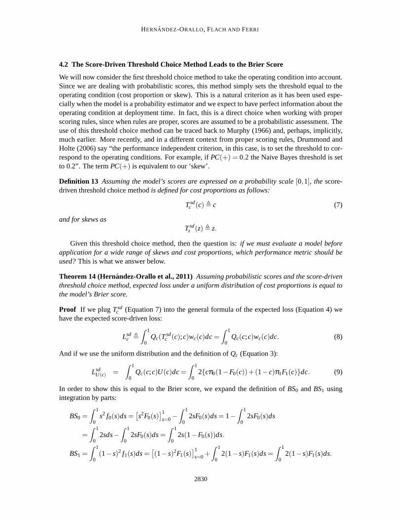
4.2 The Score-Driven Threshold Choice Method Leads to the Brier Score
We will now consider the first threshold choice method to take the operating condition into account.Since we are dealing with probabilistic scores, this method simply sets the threshold equal to theoperating condition (cost proportion or skew). This is a natural criterionas it has been used espe-cially when the model is a probability estimator and we expect to have perfect information about theoperating condition at deployment time. In fact, this is a direct choice when working with properscoring rules, since when rules are proper, scores are assumed to bea probabilistic assessment. Theuse of this threshold choice method can be traced back to Murphy (1966) and, perhaps, implicitly,much earlier. More recently, and in a different context from proper scoring rules, Drummond andHolte (2006) say “the performance independent criterion, in this case, isto set the threshold to cor-respond to the operating conditions. For example, ifPC(+) = 0.2 the Naive Bayes threshold is setto 0.2”. The termPC(+) is equivalent to our ‘skew’.
Definition 13 Assuming the model’s scores are expressed on a probability scale[0,1], thescore-driven threshold choice methodis defined for cost proportions as follows:
Tsdc (c), c (7)
and for skews asTsd
z (z), z.
Given this threshold choice method, then the question is:if we must evaluate a model beforeapplication for a wide range of skews and cost proportions, which performance metric should beused?This is what we answer below.
Theorem 14 (Hernandez-Orallo et al., 2011)Assuming probabilistic scores and the score-driventhreshold choice method, expected loss under a uniform distribution of cost proportions is equal tothe model’s Brier score.
Proof If we plug Tsdc (Equation 7) into the general formula of the expected loss (Equation 4) we
have the expected score-driven loss:
Lsdc ,
∫ 1
0Qc(T
sdc (c);c)wc(c)dc=
∫ 1
0Qc(c;c)wc(c)dc. (8)
And if we use the uniform distribution and the definition ofQc (Equation 3):
LsdU(c) =
∫ 1
0Qc(c;c)U(c)dc=
∫ 1
02{cπ0(1−F0(c))+(1−c)π1F1(c)}dc. (9)
In order to show this is equal to the Brier score, we expand the definition ofBS0 andBS1 usingintegration by parts:
BS0 =∫ 1
0s2 f0(s)ds=
[
s2F0(s)]1
s=0−∫ 1
02sF0(s)ds= 1−
∫ 1
02sF0(s)ds
=∫ 1
02sds−
∫ 1
02sF0(s)ds=
∫ 1
02s(1−F0(s))ds.
BS1 =∫ 1
0(1−s)2 f1(s)ds=
[
(1−s)2F1(s)]1
s=0+∫ 1
02(1−s)F1(s)ds=
∫ 1
02(1−s)F1(s)ds.
2830

A UNIFIED V IEW OF PERFORMANCEMETRICS
Taking their weighted average, we obtain
BS= π0BS0+π1BS1 =∫ 1
0{π02s(1−F0(s))+π12(1−s)F1(s)}ds. (10)
which, after reordering of terms and change of variable, is the same expression as Equation (9).
It is now clear why we just put the Brier score from Table 1 as the expected loss in Table 2. Wecalculated the expected loss for the score-driven threshold choice method for a uniform distributionof cost proportions as its Brier score.
Theorem 14 was obtained by Hernandez-Orallo et al. (2011) (the threshold choice method therewas called ‘probabilistic’) but it is not completely new in itself. Murphy (1966) found a similar rela-tion to expected utility (in our notation,−(1/4)PS+(1/2)(1+π0), where the so-called probabilityscorePS= 2BS). Apart from the sign (which is explained because Murphy works with utilitiesand we work with costs), the difference in the second constant term is explained because Murphy’sutility (cost) model is based on a cost matrix where we have a cost for one ofthe classes (in meteo-rology the class ‘protect’) independently of whether we have a right or wrong prediction (‘adverse’or ‘good’ weather). The only case in the matrix with a 0 cost is when we have‘good’ weather and‘no protect’. It is interesting to see that the result only differs by a constant term, which supports theidea that whenever we can express the operating condition with a cost proportion or skew, the resultswill be portable to each situation with the inclusion of some constant terms (which are the same forall classifiers). In addition to this result, it is also worth mentioning another work by Murphy (1969)where he makes a general derivation for the Beta distribution.
After Murphy, in the last four decades, there has been extensive work on the so-called properscoring rules, where several utility (cost) models have been used and several distributions for the costhave been used. This has led to relating Brier score (square loss), logarithmic loss, 0-1 loss and otherlosses which take the scores into account. For instance, Buja et al. (2005) give a comprehensiveaccount of how all these losses can be obtained as special cases of theBeta distribution. The resultgiven in Theorem 14 would be a particular case for the uniform distribution(which is a specialcase of the Beta distribution) and a variant of Murphy’s results. In fact,theBSdecomposition canalso be connected to more general decompositions of Bregman divergences (Reid and Williamson,2011). Nonetheless, it is important to remark that the results we have just obtained in Section 4.1(and those we will get in Section 5) are new because they are not obtainedby changing the costdistribution but rather by changing the threshold choice method. The threshold choice method used(the score-driven one) is not put into question in the area of proper scoring rules. But Theorem 14can now be seen as a result which connects these two different dimensions: cost distribution andthreshold choice method, so placing the Brier score at an even more predominant role.
Hernandez-Orallo et al. (2011) derive an equivalent result using empirical distributions. In thatpaper we show how the loss can be plotted in cost space, leading to theBrier curvewhose areaunderneath is the Brier score.
Finally, using skews we arrive at the prior-independent version of theBrier score.
Corollary 15 LsdU(z) = uBS= (BS0+BS1)/2.
It is interesting to analyse the relation betweenLsuU(c) andLsd
U(c) (similarly betweenLsuU(z) and
LsdU(z)). Since the former gives theMAE and the second gives the Brier score (which is the MSE),
2831

HERNANDEZ-ORALLO , FLACH AND FERRI
from the definitions ofMAE and Brier score, we get that, assuming scores are between 0 and 1:
MAE= LsuU(c) ≥ Lsd
U(c) = BS.
uMAE= LsuU(z) ≥ Lsd
U(z) = uBS.
SinceMAE andBShave the same terms but the second squares them, and all the values which aresquared are between 0 and 1, then theBSmust be lower or equal. This is natural, since the expectedloss is lower if we get reliable information about the operating condition at deployment time. So,the difference between the Brier score andMAE is precisely the gain we can get by having (andusing) the information about the operating condition at deployment time. Notice that all this holdsregardless of the quality of the probability estimates.
Finally, the difference between the results of Section 3 (Corollary 6) and these results fits wellwith a phenomenon which is observed when trying to optimise classification models: good proba-bility estimation does not imply good classification and vice versa (see, for example, the work ofFriedman, 1997). In the context of these results, we can re-interpret this phenomenon from a newperspective. The Brier score is seen as expected loss for the score-driven threshold choice method,while accuracy assumes a fixed threshold. The expected losses shown inTable 2 are a clear exampleof this.
5. Threshold Choice Methods Using Rates
We show in this section thatAUC can be translated into expected loss for varying operating con-ditions in more than one way, depending on the threshold choice method used. We consider twothreshold choice methods, where each of them sets the threshold to achievea particular predictedpositive rate: the rate-uniform method, which sets the rate in a uniform way;and the rate-drivenmethod, which sets the rate equal to the operating condition. Some of these approaches have beenused or mentioned in the literature, but choosing or ranging over sensitivity(or, complementary,specificity) instead of ranging over therate (which is a weighted sum of sensitivity, that is,F0, and1− specificity, that is,F1). For instance, Wieand et al. (1989) take a uniform distribution on a re-stricted range of sensitivities (or, similarly, specificities, Wieand et al., 1989). Also, Hand (2010)mentions thatAUC can be seen as ‘the mean specificity value, assuming a uniform distribution forthe sensitivity’.
We recall the definition of a ROC curve and its area first.
Definition 16 The ROC curve (Swets et al., 2000; Fawcett, 2006) is defined as a plot ofF1(t) (i.e.,false positive rate at decision threshold t) on the x-axis against F0(t) (true positive rate at t) on they-axis, with both quantities monotonically non-decreasing with increasing t (remember that scoresincrease withp(1|x) and 1 stands for the negative class). The Area Under the ROC curve (AUC) isdefined as:
AUC ,
∫ 1
0F0(s)dF1(s) =
∫ +∞
−∞F0(s) f1(s)ds=
∫ +∞
−∞
∫ s
−∞f0(t) f1(s)dtds
=∫ 1
0(1−F1(s))dF0(s) =
∫ +∞
−∞(1−F1(s)) f0(s)ds=
∫ +∞
−∞
∫ +∞
sf1(t) f0(s)dtds.
Note that in this section scores are not necessarily assumed to be probabilityestimates and sosranges from−∞ to ∞.
2832
A UNIFIED V IEW OF PERFORMANCEMETRICS
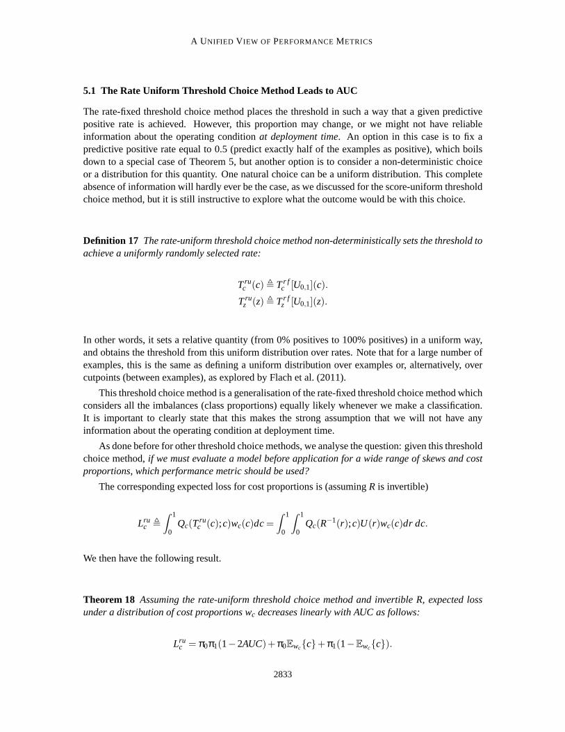
5.1 The Rate Uniform Threshold Choice Method Leads to AUC
The rate-fixed threshold choice method places the threshold in such a way that a given predictivepositive rate is achieved. However, this proportion may change, or we might not have reliableinformation about the operating conditionat deployment time. An option in this case is to fix apredictive positive rate equal to 0.5 (predict exactly half of the examples as positive), which boilsdown to a special case of Theorem 5, but another option is to consider a non-deterministic choiceor a distribution for this quantity. One natural choice can be a uniform distribution. This completeabsence of information will hardly ever be the case, as we discussed forthe score-uniform thresholdchoice method, but it is still instructive to explore what the outcome would be withthis choice.
Definition 17 The rate-uniform threshold choice method non-deterministically sets the threshold toachieve a uniformly randomly selected rate:
Truc (c), Tr f
c [U0,1](c).
Truz (z), Tr f
z [U0,1](z).
In other words, it sets a relative quantity (from 0% positives to 100% positives) in a uniform way,and obtains the threshold from this uniform distribution over rates. Note thatfor a large number ofexamples, this is the same as defining a uniform distribution over examples or, alternatively, overcutpoints (between examples), as explored by Flach et al. (2011).
This threshold choice method is a generalisation of the rate-fixed threshold choice method whichconsiders all the imbalances (class proportions) equally likely whenever we make a classification.It is important to clearly state that this makes the strong assumption that we will nothave anyinformation about the operating condition at deployment time.
As done before for other threshold choice methods, we analyse the question: given this thresholdchoice method,if we must evaluate a model before application for a wide range of skews and costproportions, which performance metric should be used?
The corresponding expected loss for cost proportions is (assumingR is invertible)
Lruc ,
∫ 1
0Qc(T
ruc (c);c)wc(c)dc=
∫ 1
0
∫ 1
0Qc(R
−1(r);c)U(r)wc(c)dr dc.
We then have the following result.
Theorem 18 Assuming the rate-uniform threshold choice method and invertible R, expected lossunder a distribution of cost proportions wc decreases linearly with AUC as follows:
Lruc = π0π1(1−2AUC)+π0Ewc{c}+π1(1−Ewc{c}).
2833

HERNANDEZ-ORALLO , FLACH AND FERRI
Proof First of all we note thatr =R(t) and henceU(r)dr =R′(t)dt = {π0 f0(t)+π1 f1(t)}dt. Underthe same change of variable,Qc(R−1(r);c) =Qc(t;c) = 2{cπ0(1−F0(t))+(1−c)π1F1(t)}. Hence:
Lruc =
∫ 1
0
∫ ∞
−∞{cπ0(1−F0(t))+(1−c)π1F1(t)}wc(c){π0 f0(t)+π1 f1(t)}dt dc
=∫ ∞
−∞
∫ 1
02{cπ0(1−F0(t))+(1−c)π1F1(t)}{π0 f0(t)+π1 f1(t)}wc(c)dc dt
=∫ ∞
−∞2{Ewc{c}π0(1−F0(t))+(1−Ewc{c})π1F1(t)}{π0 f0(t)+π1 f1(t)}dt
= 2π0π1Ewc{c}∫ ∞
−∞(1−F0(t)) f1(t)dt+2π0π1(1−Ewc{c})
∫ ∞
−∞F1(t) f0(t)dt
+2π20Ewc{c}
∫ ∞
−∞(1−F0(t)) f0(t) dt+2π2
1(1−Ewc{c})∫ ∞
−∞F1(t) f1(t) dt.
The first two integrals in this last expression are both equal to 1−AUC. The remaining two integralsreduce to a constant:
∫ ∞
−∞(1−F0(t)) f0(t) dt =−
∫ 0
1(1−F0(t)) d(1−F0(t)) = 1/2.
∫ ∞
−∞F1(t) f1(t) dt =
∫ 1
0F1(t) dF1(t) = 1/2.
Putting everything together we obtain
Lruc = 2π0π1Ewc{c}(1−AUC)+2π0π1(1−Ewc{c})(1−AUC)+π2
0Ewc{c}+π21(1−Ewc{c})
= 2π0π1(1−AUC)+π20Ewc{c}+π2
1(1−Ewc{c})
= π0π1(1−2AUC)+π0π1+π20Ewc{c}+π2
1(1−Ewc{c})
= π0π1(1−2AUC)+π0π1Ewc{c}+π20Ewc{c}+π0π1(1−Ewc{c})+π2
1(1−Ewc{c})
and the result follows.
The following two results were originally obtained by Flach, Hernandez-Orallo, and Ferri(2011) for the special case of uniform cost and skew distributions. Weare grateful to David Handfor suggesting that the earlier results might be generalised.
Corollary 19 Assuming the rate-uniform threshold choice method, invertible R, and a distributionof cost proportions wc with expected valueEwc{c} = 1/2, expected loss decreases linearly withAUC as follows:
LruE{c}=1/2 = π0π1(1−2AUC)+1/2.
Corollary 20 For any distribution of skews wz, assuming the rate-uniform threshold choice methodand invertible R, expected loss decreases linearly with AUC as follows:
Lruz = (1−2AUC)/4+1/2.
2834
A UNIFIED V IEW OF PERFORMANCEMETRICS
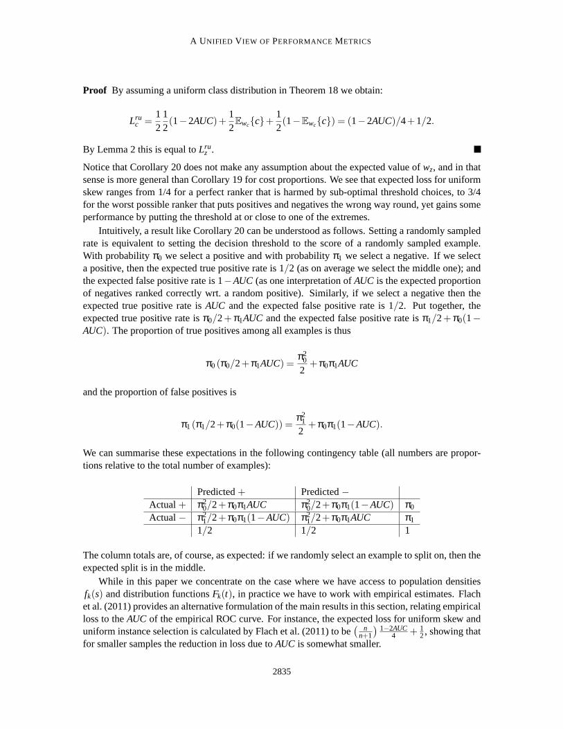
Proof By assuming a uniform class distribution in Theorem 18 we obtain:
Lruc =
12
12(1−2AUC)+
12Ewc{c}+
12(1−Ewc{c}) = (1−2AUC)/4+1/2.
By Lemma 2 this is equal toLruz .
Notice that Corollary 20 does not make any assumption about the expected value ofwz, and in thatsense is more general than Corollary 19 for cost proportions. We see that expected loss for uniformskew ranges from 1/4 for a perfect ranker that is harmed by sub-optimal threshold choices, to 3/4for the worst possible ranker that puts positives and negatives the wrong way round, yet gains someperformance by putting the threshold at or close to one of the extremes.
Intuitively, a result like Corollary 20 can be understood as follows. Settinga randomly sampledrate is equivalent to setting the decision threshold to the score of a randomly sampled example.With probabilityπ0 we select a positive and with probabilityπ1 we select a negative. If we selecta positive, then the expected true positive rate is 1/2 (as on average we select the middle one); andthe expected false positive rate is 1−AUC (as one interpretation ofAUC is the expected proportionof negatives ranked correctly wrt. a random positive). Similarly, if we select a negative then theexpected true positive rate isAUC and the expected false positive rate is 1/2. Put together, theexpected true positive rate isπ0/2+π1AUC and the expected false positive rate isπ1/2+π0(1−AUC). The proportion of true positives among all examples is thus
π0(π0/2+π1AUC) =π2
0
2+π0π1AUC
and the proportion of false positives is
π1(π1/2+π0(1−AUC)) =π2
1
2+π0π1(1−AUC).
We can summarise these expectations in the following contingency table (all numbers are propor-tions relative to the total number of examples):
Predicted+ Predicted−Actual+ π2
0/2+π0π1AUC π20/2+π0π1(1−AUC) π0
Actual− π21/2+π0π1(1−AUC) π2
1/2+π0π1AUC π1
1/2 1/2 1
The column totals are, of course, as expected: if we randomly select an example to split on, then theexpected split is in the middle.
While in this paper we concentrate on the case where we have access to population densitiesfk(s) and distribution functionsFk(t), in practice we have to work with empirical estimates. Flachet al. (2011) provides an alternative formulation of the main results in this section, relating empiricalloss to theAUC of the empirical ROC curve. For instance, the expected loss for uniform skew anduniform instance selection is calculated by Flach et al. (2011) to be
(
nn+1
)
1−2AUC4 + 1
2, showing thatfor smaller samples the reduction in loss due toAUC is somewhat smaller.
2835

HERNANDEZ-ORALLO , FLACH AND FERRI
5.2 The Rate-Driven Threshold Choice Method Leads to AUC
Naturally, if we can have precise information of the operating condition at deployment time, wecan use the information about the skew or cost to adjust the rate of positives and negatives to thatproportion. This leads to a new threshold selection method: if we are given skew (or cost proportion)z (or c), we choose the thresholdt in such a way that we get a proportion ofz (or c) positives. Thisis an elaboration of the rate-fixed threshold choice method whichdoestake the operating conditioninto account.
Definition 21 Therate-driven threshold choice methodfor cost proportions is defined as
Trdc (c), Tr f
c [c](c) = R−1(c). (11)
The rate-driven threshold choice method for skews is defined as
Trdz (z), Tr f
z [z](z) = R−1z (z).
Given this threshold choice method, the question is again:if we must evaluate a model beforeapplication for a wide range of skews and cost proportions, which performance metric should beused?This is what we answer below.
If we plug Trdc (Equation 11) into the general formula of the expected loss for a range ofcost
proportions (Equation 4) we have:
Lrdc ,
∫ 1
0Qc(T
rdc (c);c)wc(c)dc.
And now, from this definition, if we use the uniform distribution forwc(c), we obtain this newresult.
Theorem 22 Expected loss for uniform cost proportions using the rate-driven threshold choicemethod is linearly related to AUC as follows:
LrdU(c) = π1π0(1−2AUC)+1/3.
Proof
LrdU(c) =
∫ 1
0Qc(T
rdc (c);c)U(c)dc=
∫ 1
0Qc(R
−1(c);c)dc
= 2∫ 1
0{cπ0(1−F0(R
−1(c)))+(1−c)π1F1(R−1(c))}dc
= 2∫ 1
0{cπ0−cπ0F0(R
−1(c)))+π1F1(R−1(c))−cπ1F1(R
−1(c))}dc.
Sinceπ0F0(R−1(c)))+π1F1(R−1(c)) = R(R−1(c)) = c,
LrdU(c) = 2
∫ 1
0{cπ0−c2+π1F1(R
−1(c))}dc
= π0−23+2π1
∫ 1
0F1(R
−1(c))dc.
2836

A UNIFIED V IEW OF PERFORMANCEMETRICS
Taking the rightmost term and using the change of variableR−1(c) = t we havec= R(t) and hencedc= R′(t)dt = {π0 f0(t)+π1 f1(t)}dt = R′(t)dt, and thus this term is rewritten as
2π1
∫ 1
0F1(R
−1(c))dc = 2π1
∫ ∞
∞F1(t){π0 f0(t)+π1 f1(t)}dt
= 2π1π0
∫ 1
0F1(t)dF0(t)+2π2
1
∫ 1
0F1(t)dF1(t)
= 2π1π0(1−AUC)+2π2112= 2π1π0(1−AUC)+π1(1−π0).
Putting everything together we have:
LrdU(c) = π0−
23+2π1π0(1−AUC)+π1(1−π0)
=13+π1π0(1−2AUC).
Now we can unveil and understand how we obtained the results for the expected loss in Table 2for the rate-driven method. We just took theAUC of the models and applied the previous formula:π1π0(1−2AUC)+ 1
3.
Corollary 23 Expected loss for uniform skews using the rate-driven threshold choice method islinearly related to AUC as follows:
LrdU(z) = (1−2AUC)/4+1/3.
If we compare Corollary 20 with Corollary 23, we see thatLruU(z) > Lrd
U(z), more precisely:
LruU(z) = (1−2AUC)/4+1/2= Lrd
U(z)+1/6.
So we see that taking the operating condition into account when choosing thresholds based onrates reduces the expected loss with 1/6, regardless of the quality of the modelas measured byAUC.This term is clearly not negligible and demonstrates that the rate-driven threshold choice method issuperior to the rate-uniform method. Figure 3 illustrates this. Logically,Lrd
U(c) andLrdU(z) work upon
information about the operating condition at deployment time, whileLruU(c) andLru
U(z) may be suitedwhen this information is unavailable or unreliable.
6. The Optimal Threshold Choice Method
The last threshold choice method we investigate is based on the optimistic assumption that (1)we are having complete information about the operating condition (class proportions and costs) atdeployment time and (2) we are able to use that information (also at deploymenttime) to choosethe threshold that will minimise the loss using the current model. ROC analysis is precisely basedon these two points since we can calculate the threshold which gives the smallest loss by using theskew and the convex hull.
This threshold choice method, denoted byToc , is defined as follows:
2837

HERNANDEZ-ORALLO , FLACH AND FERRI
Figure 3: Illustration of the rate-driven threshold choice method. We assume uniform misclassifi-cation costs (c0 = c1 = 1), and hence skew is equal to the proportion of positives (z= π0).The majority class is class 1 on the left and class 0 on the right. Unlike the rate-uniformmethod, the rate-driven method is able to take advantage of knowing the majorityclass,leading to a lower expected loss.
Definition 24 The optimal threshold choice method is defined as:
Toc (c) , argmin
t{Qc(t;c)}= argmin
t2{cπ0(1−F0(t))+(1−c)π1F1(t)} (12)
and similarly for skews:
Toz (z), argmin
t{Qz(t;z)}.
Note that in both cases, the argmin will typically give a range (interval) of values which give thesame optimal value. So these methods can be considered non-deterministic. This threshold choicemethod is analysed by Fawcett and Provost (1997), and used by Drummond and Holte (2000, 2006)for defining their cost curves and by Hand (2009) to define a new performance metric.
If we plug Equations (12) and (3) into Equation (4) using a uniform distribution for cost propor-tions, we get:
LoU(c) =
∫ 1
0Qc(argmin
t{Qc(t,c)};c)dc=
∫ 1
0min
t{Qc(t;c)}dc
=∫ 1
0min
t{2cπ0(1−F0(t))+2(1−c)π1F1(t)}dc. (13)
The connection with the convex hull of a ROC curve (ROCCH) is straightforward. The convexhull is a construction over the ROC curve in such a way that all the points on the convex hullhave minimum loss for some choice ofc or z. This means that we restrict attention to theoptimalthreshold for a given cost proportionc, as derived from Equation (12).
2838
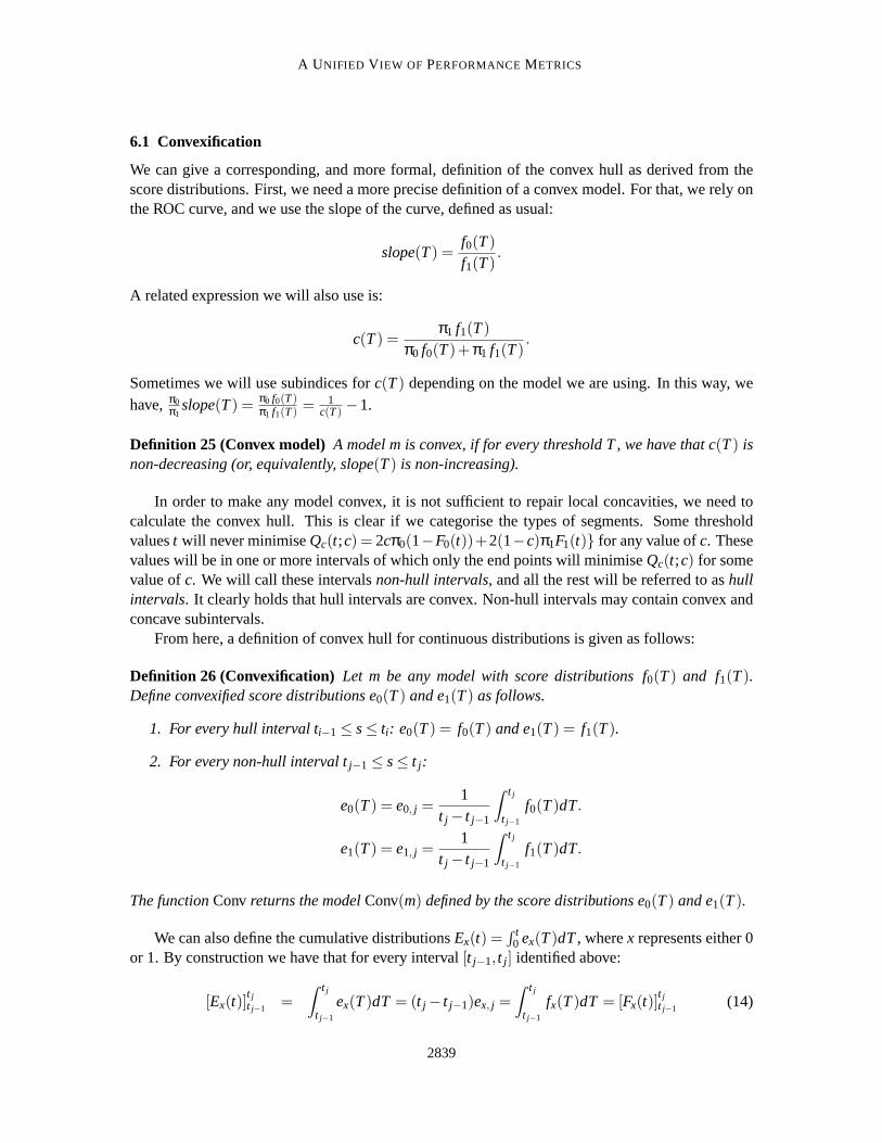
A UNIFIED V IEW OF PERFORMANCEMETRICS
6.1 Convexification
We can give a corresponding, and more formal, definition of the convex hull as derived from thescore distributions. First, we need a more precise definition of a convex model. For that, we rely onthe ROC curve, and we use the slope of the curve, defined as usual:
slope(T) =f0(T)f1(T)
.
A related expression we will also use is:
c(T) =π1 f1(T)
π0 f0(T)+π1 f1(T).
Sometimes we will use subindices forc(T) depending on the model we are using. In this way, wehave,π0
π1slope(T) = π0 f0(T)
π1 f1(T)= 1
c(T) −1.
Definition 25 (Convex model) A model m is convex, if for every threshold T , we have that c(T) isnon-decreasing (or, equivalently, slope(T) is non-increasing).
In order to make any model convex, it is not sufficient to repair local concavities, we need tocalculate the convex hull. This is clear if we categorise the types of segments.Some thresholdvaluest will never minimiseQc(t;c) = 2cπ0(1−F0(t))+2(1−c)π1F1(t)} for any value ofc. Thesevalues will be in one or more intervals of which only the end points will minimiseQc(t;c) for somevalue ofc. We will call these intervalsnon-hull intervals, and all the rest will be referred to ashullintervals. It clearly holds that hull intervals are convex. Non-hull intervals may contain convex andconcave subintervals.
From here, a definition of convex hull for continuous distributions is given as follows:
Definition 26 (Convexification) Let m be any model with score distributions f0(T) and f1(T).Define convexified score distributions e0(T) and e1(T) as follows.
1. For every hull interval ti−1 ≤ s≤ ti : e0(T) = f0(T) and e1(T) = f1(T).
2. For every non-hull interval tj−1 ≤ s≤ t j :
e0(T) = e0, j =1
t j − t j−1
∫ t j
t j−1
f0(T)dT.
e1(T) = e1, j =1
t j − t j−1
∫ t j
t j−1
f1(T)dT.
The functionConvreturns the modelConv(m) defined by the score distributions e0(T) and e1(T).
We can also define the cumulative distributionsEx(t) =∫ t
0 ex(T)dT, wherex represents either 0or 1. By construction we have that for every interval[t j−1, t j ] identified above:
[Ex(t)]t jt j−1
=∫ t j
t j−1
ex(T)dT = (t j − t j−1)ex, j =∫ t j
t j−1
fx(T)dT = [Fx(t)]t jt j−1
(14)
2839

HERNANDEZ-ORALLO , FLACH AND FERRI
and so the convexified score distributions are proper distributions. Furthermore, since the new scoredistributions are constant in the convexified intervals—and hence monotonically non-decreasing forthe newc(T), denoted bycConv(m)(T)—so is
cConv(m)(T) = c j =π1e1, j
π0e0, j +π1e1, j.
It follows that Conv(m) is everywhere convex. In addition,
Theorem 27 Optimal loss is invariant underConv, that is: LoU(c)(Conv(m)) = Lo
U(c)(m) for everym.
Proof By Equation (13) we have that optimal loss is:
LoU(c)(m) =
∫ 1
0min
t{2cπ0(1−F0(t))+2(1−c)π1F1(t)}dc.
By definition, the hull intervals have not been modified by Conv(m). Only the non-hull intervalshave been modified. A non-hull interval was defined as those where there is not which minimisesQc(t;c) = 2cπ0(1−F0(t))+2(1−c)π1F1(t)} for any value ofc, and only the endpoints attained theminimum. Consequently, we only need to show that the newe0(T) ande1(T) do not introduce anynew minima.
We now focus on each non-hull segment(t j−1, t j) using the definition of Conv. We only need tocheck the expression for the minimum:
mint j≤t≤t j−1
{2cπ0(1−E0(t))+2(1−c)π1E1(t)}.
From Equation (14) we derive thatEx(t) = Ex(t j−1)+ (t j − t j−1)ex, j inside the interval (they arestraight lines in the ROC curve), and we can see that the expression to be minimised is constant (itdoes not depend ont). Since the end points were the old minima and were equal, we see that thisexpression cannot find new minima.
It is not difficult to see that if we plot Conv(m) in the cost space defined by Drummond and Holte(2006) withQz(t;z) on they-axis against skewzon thex-axis, we have a cost curve. Its area is thenthe expected loss for the optimal threshold choice method. In other words, this is the area under the(optimal) cost curve. Similarly, the new performance metricH introduced by Hand (2009) is simplya rescaled version of the area under the optimal cost curve using theβ2,2 distribution instead of theβ1,1 (i.e., uniform) distribution, and using cost proportions instead of skews (so being dependent toclass priors). This is further discussed by Flach et al. (2011). While allof these distributions aresymmetric, the Beta distribution can be non-symmetric if required by a specific application. In fact,Hand and Anagnostopoulos (2012) suggest that the parameters of the distribution should be linkedto class proportionπ0.
6.2 The Optimal Threshold Choice Method Leads to Refinement Loss
Once again, the question now must be stated clearly. Assume that the optimal threshold choicemethod is set as the method we will use for every application of our model. Furthermore, assume
2840

A UNIFIED V IEW OF PERFORMANCEMETRICS
that each and every application of the model is going to find the perfect threshold. Then,if wemust evaluate a model before application for a wide range of skews and cost proportions, whichperformance metric should be used?In what follows, we will find the answer by relating thisexpected loss with a genuine performance metric: refinement loss. We will now introduce thisperformance metric.
The Brier score, being a sum of squared probabilistic residuals, can bedecomposed in variousways. The most common decomposition of the Brier score is due to Murphy (1973) and decomposesthe Brier score into Reliability, Resolution and Uncertainty. Frequently, the twolatter componentsare joined together and the decomposition gives two terms: calibration loss andrefinement loss.
This decomposition is usually applied to empirical distributions, requiring a binning of thescores. Scores are assumed to be probability estimates in the interval[0,1]. The decompositionis based on a partitionPD = {b j} j=1..B whereD is the data set,B the number of bins, and each binis denoted byb j ⊂ D. Since it is a partition
⋃Bj=1b j = D. With this partition the decompoistion is:
BS≈ CLPD +RLPD =1n
B
∑j=1
|b j |(
sb j −yb j
)2+
1n
B
∑j=1
|b j |yb j
(
1−yb j
)
.
Here we use the notationsb j =1|b j |
∑i∈b jsi andyb j =
1|b j |
∑i∈b jyi for the average predicted scores and
the average actual classes respectively for binb j .For many partitions the empirical decomposition is not exact. It is only exact for partitions
which are coarser than the partition induced by the ROC curve (i.e., ties cannot be spread overdifferent partitions), as shown by Flach and Matsubara (2007). We denote byCLROC andRLROC
the calibration loss and the refinement loss, respectively, using the segments of the empirical ROCcurve as bins. In this case,BS= CLROC+RLROC.
In this paper we will use a variant of the above decomposition based on the ROC convex hullof a model. In this decomposition, we take each bin as each segment in the convex hull. Naturally,the number of bins in this decomposition is lower or equal than the number of binsin the ROCdecomposition. In fact, we may find different values ofsi in the same bin. In some way, we canthink about this decomposition as an optimistic/optimal version of the ROC decomposition, as Flachand Matsubara (2007, Th. 3) show. We denote byCLROCCH andRLROCCH the calibration loss andthe refinement loss, respectively, using the segments of the convex hull of the empirical ROC curveas bins (Flach et al., 2011).
We can define the same decomposition in continuous terms considering Definition8. We cansee that in the continuous case, the partition is irrelevant. Any partition will give the same result,since the composition of consecutive integrals is the same as the whole integral.
Theorem 28 The continuous decomposition of the Brier Score, BS= CL+RL, is exact and givesCL and RL as follows.
CL=∫ 1
0
(s(π0 f0(s)+π1 f1(s))−π1 f1(s))2
π0 f0(s)+π1 f1(s)ds.
RL=∫ 1
0
π1 f1(s)π0 f0(s)π0 f0(s)+π1 f1(s)
ds.
2841
HERNANDEZ-ORALLO , FLACH AND FERRI
Proof
BS=∫ 1
0
[
s2π0 f0(s)+(1−s)2π1 f1(s)]
ds
=∫ 1
0
[
s2(π0 f0(s)+π1 f1(s))−2sπ1 f1(s)+π1 f1(s)]
ds
=∫ 1
0
s2(π0 f0(s)+π1 f1(s))2−2s(π0 f0(s)+π1 f1(s))π1 f1(s)+π1 f1(s)(π1 f1(s)+π0 f0(s))(π0 f0(s)+π1 f1(s))
ds
=∫ 1
0
(s(π0 f0(s)+π1 f1(s))−π1 f1(s))2+π1 f1(s)π0 f0(s)
π0 f0(s)+π1 f1(s)ds
=∫ 1
0
(s(π0 f0(s)+π1 f1(s))−π1 f1(s))2
π0 f0(s)+π1 f1(s)ds+
∫ 1
0
π1 f1(s)π0 f0(s)π0 f0(s)+π1 f1(s)
ds.
This proof keeps the integral from start to end. That means that the decomposition is not onlytrue for the integral as a whole, but also pointwise for every single scores. Note thatyb j in the
empirical case (see Definition 15) corresponds toc(s) = π1 f1(s)π0 f0(s)+π1 f1(s)
(as given by Equation 14) inthe continuous case above, and also note thatsb j corresponds to the cardinalityπ0 f0(s)+π1 f1(s).The decomposition for empirical distributions as introduced by Murphy (1973) is still predominantfor any reference to the decomposition. To our knowledge this is the first explicit derivation of acontinuous version of the decomposition.
And now we are ready for relating the optimal threshold choice method with a performancemetric as follows:
Theorem 29 For every convex model m, we have that:
LoU(c)(m) = RL(m).
The proof of this theorem is found in the appendix as Theorem 48.
Corollary 30 For every model m the expected loss for the optimal threshold choice method LoU(c) is
equal to the refinement loss using the convex hull.
LoU(c)(m) = RL(Conv(m)), RLConv(m).
Proof We haveLoU(c)(m) = Lo
U(c)(Conv(m)) by Theorem 27, andLoU(c)(Conv(m)) = RL(Conv(m))
by Theorem 29 and the convexity of Conv(m).
It is possible to obtain a version of this theorem for empirical distributions which states thatLoU(c) =
RLROCCH whereRLROCCH is the refinement loss of the empirical distribution using the segments ofthe convex hull for the decomposition.
Before analysing what the meaning of this threshold choice method is and howit relates to therest, we have to consider whether this threshold choice method is realistic or not. In the beginning ofthis section we said that the optimal method assumes that (1) we are having complete informationabout the operating condition at deployment time and (2) we are able to use that information tochoose the threshold that will minimise the loss at deployment time.
2842

A UNIFIED V IEW OF PERFORMANCEMETRICS
While (1) is not always true, there are many occasions where we know thecosts and distribu-tions at application time. This is the base of the score-driven and rate-driven methods. However,having this information does not mean that the optimal threshold for a data set (e.g., the training orvalidation data set) ensures an optimal choice for a test set (2). Drummond and Holte (2006) areconscious of this problem and they reluctantly rely on a threshold choice method which is basedon “the ROC convex hull [...] only if this selection criterion happens to make cost-minimizing se-lections, which in general it will not do”. But even if these cost-minimising selections are done, asmentioned above, it is not clear how reliable they are for a test data set. As Drummond and Holte(2006, p. 122) recognise: “there are few examples of the practical application of this technique.One example is given by Fawcett and Provost (1997), in which the decision threshold parameterwas tuned to be optimal, empirically, for the test distribution”.
In the example shown in Table 2 in Section 1, the evaluation technique was training and test.However, with cross-validation, the convex hull cannot be estimated reliably in general, and thethresholds derived from each fold might be inconsistent. Even with a largevalidation data set, thedecision threshold may be suboptimal. This is one of the reasons why the areaunder the convex hullhas not been used as a performance metric. In any case, we can calculate the values as an optimisticlimit, leading toLo
U(c) = RLROCCH= 0.0953 for modelA and 0.2094 for modelB.
7. Relating Performance Metrics
So far, we have repeatedly answered the following question: “If threshold choice methodX is used,which is the corresponding performance metric?” The answers are summarised in Table 4. Theseven threshold choice methods are shown in the first column (the two fixed methods are groupedin the same row). The integrated view of performance metrics for classification is given by thenext two columns. The expected loss of a model for a uniform distribution ofcost proportions orskews for each of these seven threshold choice methods produces mostof the common performancemetrics in classification: 0-1 loss (either weighted or unweighted accuracy), the Mean AbsoluteError (equivalent to Mean Probability Rate), the Brier score,AUC (which equals the Wilcoxon-Mann-Whitney statistic and the Kendall tau distance of the model to the perfectmodel, and islinearly related to the Gini coefficient) and, finally, the refinement loss usingthe bins given by theconvex hull.
All the threshold choice methods seen in this paper consider model scores indifferent ways.Some of them disregard the score, since the threshold is fixed, some othersconsider the ‘magnitude’of the score as an (accurate) estimated probability, leading to the score-based methods, and othersconsider the ‘rank’, ‘rate’ or ‘proportion’ given by the scores, leading to the rate-based methods.Since the optimal threshold choice is also based on the convex hull, it is apparently more related tothe rate-based methods. This is consistent with the taxonomy proposed by Ferri et al. (2009) basedon correlations over more than a dozen performance metrics, where threefamilies of metrics wererecognised: performance metrics which account for the quality of classification (such as accuracy),performance metrics which account for a ranking quality (such asAUC), and performance metricswhich evaluate the quality of scores or how well the model does in terms of probability estimation(such as the Brier score or logloss).
This suggests that the way scores are distributed is crucial in understanding the differences andconnections between these metrics. In addition, this may shed light on which threshold choicemethod is best. We have already seen some relations, such asLsu
U(c) ≥ LsdU(c), andLru
U(c) > LrdU(c), but
2843

HERNANDEZ-ORALLO , FLACH AND FERRI
Thresholdchoicemethod
Cost proportions Skews Equivalent (or related) performancemetrics
fixed Ls fU(c) = 1−Acc Ls f
U(z) = 1−uAcc 0-1 loss: Weighted and unweighted accuracy.
score-uniform
LsuU(c) = MAE Lsu
U(z) = uMAE Absolute error, Average score,pAUC(Ferri et al., 2005), Probability Rate (Ferri et al., 2009).
score-driven LsdU(c) = BS Lsd
U(z) = uBS Brier score (Brier, 1950), Mean Squared Error (MSE).
rate-uniform LruU(c) = π0π1(1−2AUC)+ 1
2 LruU(z) =
1−2AUC4 + 1
2 AUC (Swets et al., 2000) and variants (wAUC) (Fawcett,2001; Ferri et al., 2009), Kendall tau, WMW statistic,Gini coefficient.
rate-driven LrdU(c) = π0π1(1−2AUC)+ 1
3 LrdU(z) =
1−2AUC4 + 1
3 AUC (Swets et al., 2000) and variants (wAUC) (Fawcett,2001; Ferri et al., 2009), Kendall tau, WMW statistic,Gini coefficient.
optimal LoU(c) = RLConv Lo
U(z) = uRLConv ROCCH Refinement loss (Flach and Matsubara, 2007),Refinement Loss (Murphy, 1973), Area under the CostCurve (‘Total Expected Cost’) (Drummond and Holte,2006), Hand’s H (Hand, 2009).
Table 4: Threshold choice methods and their expected loss for cost proportions and skews. Theuin uAcc, uMAE, uBSanduRLmean that these metrics are unweighted, that is, calculatedas ifπ0 = π1, while thew in wAUCrefers to a weighted version of the AUC, and thex-axisandy-axis are proportional toπ0 andπ1.
what aboutLsdU(c) andLrd
U(c)? Are they comparable? And what aboutLoU(c)? It gives the minimum
expected loss by definition over the training (or validation) data set, but when does it become a goodestimation of the expected loss for the test data set?
In order to answer these questions we need to analyse transformations onthe scores and see howthese affect the expected loss given by each threshold choice method. For the rest of the section weassume that scores are in the interval[0,1]. Given a model, its scores establish a total order overthe examples:σ = (s1,s2, ...,sn) wheresi ≤ si+1. Since there might be ties in the scores, this totalorder is not necessarily strict. A monotonic transformation is any alteration ofthe scores, such thatthe order is kept. We will consider two transformations: the evenly-spacedtransformation and PAVcalibration.
7.1 Evenly-Spaced Scores. Relating Brier Score, MAE and AUC
If we are given a ranking or order, or we are given a set of scoresbut its reliability is low, a quitesimple way to assign (or re-assign) the scores is to set them evenly-spaced (in the[0,1] interval).
Definition 31 A discrete evenly-spaced transformation is a procedureEST(σ)→ σ′ which convertsany sequence of scoresσ = (s1,s2, ...,sn) where si < si+1 into scoresσ′ = (s′1,s
′2, ...,s
′n) where s′i =
i−1n−1.
Notice that such a transformation does not affect the ranking and hencedoes not alter theAUC.The previous definition can be applied to continuous score distribution as follows:
Definition 32 A continuous evenly-spaced transformation is a any strictly monotonic transforma-tion function on the score distribution, denoted byEven, such that for the new scores s′ it holds thatP(s′ ≤ t) = t.
2844

A UNIFIED V IEW OF PERFORMANCEMETRICS
It is easy to see that EST is idempotent, that is, EST(EST(σ)) = EST(σ). So we say a set ofscoresσ is evenly-spaced if EST(σ) = σ.
Lemma 33 Given a model and data set with set of scoresσ, such that they evenly-spaced, whenn→ ∞ then we have R(t) = t.
Proof Remember that by definition the true positive rateF0(t) = P(s≤ t|0) and the false positiverateF1(t)=P(s≤ t|1). Consequently, from the definition of rate we haveR(t)= π0F0(t)+π1F1(t)=π0P(s≤ t|0)+ π1P(s≤ t|1) = P(s≤ t). But, since the scores are evenly-spaced, the number ofscores such thats≤ t is ∑n
i=1 I(si ≤ t) = ∑ni=1 I( i−1
n−1 ≤ t) with I being the indicator function (1 whentrue, 0 otherwise). This number of scores is∑tn
i=11 whenn → ∞, which clearly givestn. So theprobabilityP(s≤ t) is tn/n= t. ConsequentlyR(t) = t.
The following results connect the score-driven threshold choice methodwith the rate-driventhreshold choice method:
Theorem 34 Given a model and data set with set of scoresσ, such that they are evenly-spaced,when n→ ∞:
BS= LsdU(c) = Lrd
U(c) = π0π1(1−2AUC)+13.
Proof By Lemma 33 we haveR(t) = t, and so the rate-driven and score-driven threshold choicemethods select the same thresholds.
Corollary 35 Given a model and data set with set of scoresσ such that they are evenly-spaced,when n→ ∞:
uBS= LsdU(z) = Lrd
U(z) =1−2AUC
4+
13.
These straightforward results connectAUC and Brier score for evenly-spaced scores. This connec-tion is enlightening because it says thatAUC andBSare equivalent performance metrics (linearlyrelated) when we set the scores in an evenly-spaced way. In other words, it says thatAUC is like aBrier score which considers all the scores evenly-spaced. Although the condition is strong, this isthe first linear connection which, to our knowledge, has been establishedso far betweenAUC andthe Brier score.
Similarly, we get the same results for the score-uniform threshold choice method and the rate-uniform threshold choice method.
Theorem 36 Given a model and data set with set of scoresσ such that they are evenly-spaced,when n→ ∞:
MAE= LsuU(c) = Lru
U(c) = π0π1(1−2AUC)+12
with similar results for skews. This also connectsMAE with AUC and clarifies when they arelinearly related.
2845

HERNANDEZ-ORALLO , FLACH AND FERRI
7.2 Perfectly-Calibrated Scores. Relating BS, CL and RL
In this section we will work with a different condition on the scores. We will study what interestingconnections can be established if we assume the scores to be perfectly calibrated.
The informal definition of perfect calibration usually says that a model is calibrated when theestimated probabilities are close to the true probabilities. From this informal definition, we wouldderive that a model is perfectly calibrated if the estimated probability given bythe scores (i.e.,p(1|x)) equals the true probability. However, if this definition is applied to single instances, it im-plies not only perfect calibration but a perfect model. In order to give amore meaningful definition,the notion of calibration is then usually defined in terms of groups or bins of examples, as we did,for instance, with the Brier score decomposition. So, we need to apply this correspondence betweenestimated and true (actual) probabilities over bins. We say a bin partition is invariant on the scoresif for any two examples with the same score they are in the same bin. In other words, two equalscores cannot be in different bins (equivalence classes cannot bebroken). From here, we can give adefinition of perfect calibration:
Definition 37 (Perfectly-calibrated for empirical distribution models) A model isperfectly cal-ibratedif for any invariant bin partitionP we have that yb j = sb j for all its bins: that is, the averageactual probability equals the average estimated probability, thus making CLP = 0.
Note that it is not sufficient to haveCL= 0 for one partition, but for all the invariant partitions. Alsonotice that the bins which are generated by a ROC curve are the minimal invariant partition on thescores (i.e., the quotient set). So, we can give an alternative definition ofperfectly calibrated model:a model is perfectly calibrated if and only ifCLROC= 0. For the continuous case, the partition isirrelevant and the definition is as follows:
Definition 38 (Perfectly-calibrated for continuous distribution models) A continuous model isperfectly calibratedif and only if s= π1 f1(s)
π0 f0(s)+π1 f1(s)which is exactly c(s) given by Equation (14).
Note that the previous definition is equivalent to saying thatCL= 0, as in the empirical case, sinceCL can be rewritten as follows, following the decomposition of Theorem 28:
CL =∫ 1
0
(s(π0 f0(s)+π1 f1(s))−π1 f1(s))2
π0 f0(s)+π1 f1(s)ds
=∫ 1
0(π0 f0(s)+π1 f1(s))
(
s−π1 f1(s)
π0 f0(s)+π1 f1(s)
)2
ds.
Lemma 39 For a perfectly calibrated classifier m:
1−ss
=f0(s)f1(s)
π0
π1
and m is convex.
Proof The expression is a direct transformation of Definition 38 and convexity just follows fromDefinition 25.
2846

A UNIFIED V IEW OF PERFORMANCEMETRICS
Now that we have two proper and operational definitions of perfect calibration, we define acalibration transformation as follows.
Definition 40 Cal is a monotonic function over the scores which converts any model m into anothercalibrated model m∗ such that CL= 0 and RL is not modified.
Cal always produces a convex model, so Conv(Cal(m)) = Cal(m), but a convex model is not alwaysperfectly calibrated (e.g., a binormal model with same variances is always convex but it can beuncalibrated), so Cal(Conv(m) 6= Conv(m). This is summarised in Table 5. If the model is strictlyconvex, then Cal is strictly monotonic. An instance of the function Cal is the transformationT 7→
s= c(T) wherec(T) = π1 f1(T)π0 f0(T)+π1 f1(T)
as given by Equation (14). This transformation is shown tokeepRL unchanged in the appendix and makesCL= 0.
The previous function is defined for continuous score distributions. Thecorresponding functionfor empirical distributions is known as the Pool Adjacent Algorithm (PAV) (Ayer et al., 1955).Following Fawcett and Niculescu-Mizil (2007), thePAV function converts any modelm into anothercalibrated modelm∗ such that the following propertysb j = yb j holds for every segment in its convexhull.
Evenly-spaced Convexification Perfect Calibration
Continuous distributions Even Conv CalEmpirical distributions EST ROCCH PAV
Table 5: Transformations on scores. Perfect calibration implies a convexmodel but not vice versa.
Fawcett and Niculescu-Mizil (2007) have shown that isotonic-based calibration (Robertsonet al., 1988) is equivalent to the PAV algorithm, and closely related to ROCCH,since, for everymand data set, we have:
BS(PAV(m)) = CLROC(PAV(m))+RLROC(PAV(m)) = CLROCCH(PAV(m))+RLROCCH(PAV(m))
= RLROC(PAV(m)) = RLROCCH(PAV(m)).
It is also insightful to see that isotonic regression (calibration) is the monotonic function defined asargminf ∑(yi − f (si))
2, that is, the monotonic function over the scores which minimises the Brierscore. This leads to the same function if we use any other proper scoring function (such as logloss).
The similar expression for the continuous case is
BS(Cal(m)) = CL(Cal(m))+RL(Cal(m)) = RL(Cal(m)).
Now we analyse what happens with perfectly calibrated models for the score-driven thresholdchoice and the score-uniform threshold choice methods. This will help us understand the similaritiesand differences between the threshold choices and their relation with the optimal method. Alongthe way, we will obtain some straightforward, but interesting, results.
Theorem 41 If a model is perfectly calibrated then we have:
π0s0 = π1(1− s1) (15)
or equivalently,
π0MAE0 = π1MAE1.
2847

HERNANDEZ-ORALLO , FLACH AND FERRI
Proof For perfectly calibrated models, we have that for every bin in an invariantpartition on thescores we have thatyb j = sb j . Just taking a partition consisting of one single bin (which is aninvariant partition), we have that this is the same as saying thatπ1 = π1s1 + π0s0. This leads toπ1(1− s1) = π0s0.
Equation (15) is an interesting formula in its own right. It gives a necessarycondition forcalibration: the extent to which the average score over all examples (whichis the weighted mean ofper-class averagesπ0s0+π1s1) deviates fromπ1.
We now give a first result which connects two performance metrics:
Theorem 42 If a model is perfectly calibrated then we have:
BS= π0s0 = π1(1− s1) = MAE/2.
Proof We use the continuous decomposition (Theorem 28):
BS= CL+RL.
Since it is perfectly calibrated,CL= 0. Then we have:
BS = RL=∫ 1
0
π1 f1(s)π0 f0(s)π0 f0(s)+π1 f1(s)
ds=∫ 1
0(π1 f1(s))
(
1−π1 f1(s)
π0 f0(s)+π1 f1(s)
)
ds
=∫ 1
0
(
π1 f1(s)−[π1 f1(s)]2
π0 f0(s)+π1 f1(s)
)
ds=∫ 1
0π1 f1(s)ds−
∫ 1
0
[π1 f1(s)]2
π0 f0(s)+π1 f1(s)ds
= π1−∫ 1
0
π1 f1(s)π0 f0(s)π1 f1(s)
+1ds.
Since it is perfectly calibrated, we have, by Lemma 39:
f0(s)f1(s)
=1−s
sπ1
π0.
So:
BS = π1−∫ 1
0
π1 f1(s)π0π1
1−ss
π1π0+1
ds= π1−∫ 1
0
sπ1 f1(s)(1−s)+s
ds
= π1−π1
∫ 1
0s f1(s)ds= π1(1−
∫ 1
0s f1(s))ds= π1(1− s1).
We will now use the expressions for expected loss to analyse where this result comes fromexactly. In the following result, we see that for a calibrated model the optimal thresholdT for agiven cost proportionc is T = c, which is exactly the score-driven threshold choice method. Inother words:
2848

A UNIFIED V IEW OF PERFORMANCEMETRICS
Theorem 43 For a perfectly calibrated model:To
c (c) = Tsdc (c) = c.
Proof We first take Equation (12):
Toc (c) = argmin
t2{cπ0(1−F0(t))+(1−c)π1F1(t)}.
We calculate the derivative and equal it to 0 to gett, but we isolatec:
2{cπ0(1− f0(t))+(1−c)π1 f1(t)}= 0
c=π1 f1(t)
π0 f0(t)+π1 f1(t).
From Definition 38 (perfect calibration) we have that the right expression above equalst, so wehavet = c. The proof is identical forTsd
c .
And now we can express and relate many of the expressions for the expected loss seen so far.Starting with the expected loss for the optimal threshold choice method, that is,Lo
c (which usesTo
c ), we have, from Theorem 43, thatToc (c) = Tsd
c (c) = c when the model is perfectly calibrated.Consequently, we have the same as Equation (8), and since we know thatBS= π0s0 for perfectlycalibrated models, we have:
LoU(c) = BS= π0s0 = MAE/2.
The following theorem summarises all the previous results.
Theorem 44 For perfectly calibrated models:
LsdU(c) = Lo
U(c) = RL=Lsu
U(c)
2=
MAE2
= BS= π0s0 = π1(1−s1).
Proof SinceLsdU(c) = BSit is clear thatLsd
U(c) = π0s0, as seen above forLoU(c) as well. Additionally,
from Theorem 12, we have thatLsuU(c) = π0s0+π1(1−s1), which reduces to 2Lsu
U(c) = 2BS= 2π0s0.We also use the result of Theorem 29 which states that, in general (not just for perfectly calibratedmodels),Lo
U(c)(m) = RL(Conv(m)).
All this gives an interpretation of the optimal threshold choice method as a method which cal-culates expected loss by assuming perfect calibration. Note that this is clearly seen by the relation
LsdU(c) = Lo
U(c) =Lsu
U(c)
2 , since the loss drops to the half if we use scores to adjust to the operatingcondition. In this situation, we get the best possible result.
7.3 Choosing a Threshold Choice Method
It is enlightening to see that many of the most popular classification performance metrics are justexpected losses by changing the threshold choice method and the use of cost proportions or skews.However, it is even more revealing to see how (and under which conditions) these performance
2849

HERNANDEZ-ORALLO , FLACH AND FERRI
General relations:
LruU(c) = π0π1(1−2AUC)+
12> Lrd
U(c) = π0π1(1−2AUC)+13≥ Lo
U(c) = RLConv
LsuU(c) = MAE≥ Lsd
U(c) = BS≥ LoU(c) = RLConv
If scores are evenly-spaced:
LruU(c) = π0π1(1−2AUC)+
12= Lsu
U(c) = MAE= π0s0+π1(1−s1)
LrdU(c) = π0π1(1−2AUC)+
13= Lsd
U(c) = BS
If scores are perfectly calibrated:
LsdU(c) = Lo
U(c) = RL=Lsu
U(c)
2=
MAE2
= BS= π0s0 = π1(1−s1)
If the model has perfect ranking:
LruU(c) =
14> Lrd
U(c) =112
> LoU(c) = 0
If the model is random (andπ0 = π1):
LsuU(c) = Lsd
U(c) = LruU(c) =
12> Lrd
U(c) =13> Lo
U(c) =14
Figure 4: Comparison of losses and performance metrics, in general andunder several score con-ditions.
metrics can be related (in some cases with inequalities and in some other cases withequalities).The notion of score transformation is the key idea for these connections, and is more important thatit might seem at first sight. Some threshold choice methods can be seen as a score transformationfollowed by the score-driven threshold choice method. Even the fixed threshold choice methodcan be seen as a crisp transformation where scores are set to 1 ifsi > t and 0 otherwise. Anotherinteresting point of view is to see the values of extreme models, such as a modelwith perfect ranking(AUC= 1,RLROCCH= 0) and a random model (AUC= 0.5,RLROCCH= 0.25 whenπ0 = π1). Figure4 summarises all the relations found so far and these extreme cases.
The first apparent observation is thatLoU(c) seems the best loss, since it derives from the optimal
threshold choice method. We already argued in Section 6 that this is unrealistic. The result givenby Theorem 29 is a clear indication of this, since this makes expected loss equal to RLConv. Hence,this threshold choice method assumes that the calibration which is performed withthe convex hullover the training (or a validation data set) is going to be perfect and hold forthe test set. Figure 4also gives the impression thatLsu
U(c) andLruU(c) are so bad that their corresponding threshold choice
methods and metrics are useless. In order to refute this simplistic view, we must realise (again) thatnot every threshold choice method can be applied in every situation. Some require more information
2850

A UNIFIED V IEW OF PERFORMANCEMETRICS
or more assumptions than others. Table 6 completes Table 3 to illustrate the point. If we knowthe deployment operating condition at evaluation time, then we can fix the threshold and get theexpected loss. If we do not know this information at evaluation time, but we expect to be ableto have it and use it at deployment time, then the score-driven, rate-driven and optimal thresholdchoice methods seem the appropriate ones. Finally, if no information about the operating conditionis going to be available at any time then the score-uniform and the rate-uniformmay be alternativeoptions, which could account for a worst-case estimation.
Threshold choice method Fixed Driven by o.c. Chosen uniformlyUsing scores score-fixed (Ts f) score-driven (Tsd) score-uniform (Tsu)Using rates rate-fixed (Tr f ) rate-driven (Trd) rate-uniform (Tru)Using optimal thresholds optimal (To)Required information o.c. at evaluation time o.c. at deployment time no information
Table 6: Information which is required (and when) for the seven threshold choice methods so thatthey become reasonable (or just not totally unreasonable). Operating condition is denotedby o.c.
From the cases shown in Table 6, the methods driven by the operating condition require furtherdiscussion. The relations shown in Figure 4 illustrate that, in addition to the optimalthresholdchoice method, the other two methods that seem more competitive are the score-driven and the rate-driven. One can argue that the rate-driven threshold choice has an expected loss which is alwaysgreater than 1/12 (if AUC= 1, we get−1/4+1/3), while the others can be 0. But things are notso clear-cut.
• The score-driven threshold choice method considers that the scores are estimated probabili-ties and that they are reliable, in the tradition of proper scoring rules. So it just uses theseprobabilities to set the thresholds.
• The rate-driven threshold choice method completely ignores the scores and only considerstheir order. It assumes that the ranking is reliable while the scores are notaccurate prob-abilities. It derives the thresholds using the predictive positive rate. It can be seen as thescore-driven threshold choice method where the scores have been set evenly-spaced by atransformation.
• The optimal threshold choice method also ignores the scores completely and only considerstheir order. It assumes that the ranking is reliable while the scores are notaccurate probabili-ties. However, this method derives the thresholds by keeping the order and using the slopes ofthe segments of the convex hull (typically constructed over the training data set or a validationdata set). It can be seen as the score-driven threshold choice method where the scores havebeen calibrated by the PAV method.
Now that we better understand the meaning of the threshold choice methods we may state the diffi-cult question more clearly: given a model, which threshold choice method should we use to makeclassifications? The answer is closely related to the calibration problem. Some theoretical and ex-perimental results (Robertson et al., 1988; Ayer et al., 1955; Platt, 1999;Zadrozny and Elkan, 2001,
2851

HERNANDEZ-ORALLO , FLACH AND FERRI
2002; Niculescu-Mizil and Caruana, 2005; Niculescu-Mizil and Caruana, 2005; Bella et al., 2009;Gebel, 2009) have shown that the PAV method (also known as isotonic regression) is not frequentlythe best calibration method. Some other calibration methods could do better, such as Platt’s calibra-tion or binning averaging. In particular, it has been shown that “isotonic regression is more prone tooverfitting, and thus performs worse than Platt scaling, when data is scarce” (Niculescu-Mizil andCaruana, 2005). Even with a large validation data set which allows the construction of an accurateROC curve and an accurate convex hull, the resulting choices are not necessarily optimal for the testset, since there might be problems with outliers (Ruping, 2006). In fact, if the validation data set ismuch smaller (or biased) than the training set, the resulting probabilities can be even worse than theoriginal probabilities, as it may happen with cross-validation. So, we have tofeel free to use other(possibly better) calibration methods instead and do not stick to the PAV method just because it islinked to the optimal threshold choice method.
So the question of whether we keep the scores or not (and how we replace them in case) dependson our expectations on how well-calibrated the model is, and whether we have tools (calibrationmethods and validation data sets) to calibrate the scores.
But we can turn the previous question into a much more intelligent procedure.Calculating thethree expected losses discussed above (and perhaps the other threshold choice methods as well) pro-vides a rich source of information about how our models behave. This is what performance metricsare all about. It is only after the comparison of all the results and the availability of (validation) datasets when we can make a decision about which threshold choice method to use.
This is what we did with the example shown in Table 2 in Section 1. We evaluated themodel forseveral threshold choice methods and from there we clearly saw which models were better calibratedand we finally made a decision about which model to use and with which threshold choice methods.
In any case, note that the results and comparisons shown in Figure 4 are for expected loss; theactual loss does not necessarily follow these inequalities. In fact, the expected loss calculated over avalidation data set may not hold over the test data set, and even some threshold choice methods wehave discarded from the discussion above (the fixed ones or the score-uniform and rate-uniform, ifprobabilities or rankings are very bad respectively) could be better in some particular situations.
8. Discussion
This paper builds upon the notion of threshold choice method and the expected loss we can obtainfor a range of cost proportions (or skews) for each of the thresholdchoice methods we have inves-tigated. The links between threshold choice methods, between performance metrics, in general andfor specific score arrangements, have provided us with a much broader(and more elaborate) view ofclassification performance metrics and the way thresholds can be chosen.In this last section we linkour results to the extensive bulk of work on classification evaluation and analyse the most importantcontributions and open questions which are derived from this paper.
8.1 Related Work
One decade ago there was a scattered view of classification evaluation. Many performance metricsexisted and it was not clear what their relationships were. One first step inunderstanding some ofthese performance metrics in terms of costs was the notion of cost isometrics (Flach, 2003). Withcost isometrics, many classification metrics (and decision tree splitting criteria) are characterised byits skew landscape, that is, the slope of its isometric at any point in the ROC space. Another com-
2852

A UNIFIED V IEW OF PERFORMANCEMETRICS
prehensive view was the empirical evaluation made by Ferri et al. (2009). The analysis of Pearsonand Spearman correlations between 18 different performance metrics shows the pairs of metrics forwhich the differences are significant. However, this work does not elaborate, at least theoretically,on what exactly each metric measures, but rather on whether they give different choices in general.
In addition to these, there have been three lines of research in this area which provide furtherpieces to understand the whole picture.
• First, the notion of ‘proper scoring rules’ (which was introduced in the sixties, see for exam-ple, the work by Murphy and Winkler, 1970), has been developed to a degree (Buja et al.,2005) in which it has been shown that the Brier score (MSE loss), logloss, boosting lossand error rate (0-1 loss) are all special cases of an integral over a Beta density, and thatall these performance metrics can be understood as averages (or integrals), at least theoret-ically, over a range of cost proportions (see, e.g., the works of Gneitingand Raftery, 2007;Reid and Williamson, 2010 and Brummer, 2010), so generalising the early works by Murphyon probabilistic predictions when cost-loss ratio is unknown (Murphy, 1966, 1969). Addi-tionally, further connections have been found between proper scoringrules and distributiondivergences (f -divergences and Bregman divergences) (Reid and Williamson, 2011).
• Second, the translation of the Brier decomposition using ROC curves (Flachand Matsubara,2007) suggests a connection between the Brier score and ROC curves,and particularly be-tween refinement loss andAUC, since both are performance metrics which do not require themagnitude of the scores of the model.
• Third, an important coup d’effet has been given by Hand (2009), stating that theAUC can-not be used as a performance metric for evaluating models (for a range ofcost proportions),assuming the optimal threshold choice method, because the distribution for these cost pro-portions depends on the model. This seemed to suggest a definitive rupturebetween rankingquality and classification performance over a range of cost proportions.
Each of the three lines mentioned above provides a partial view of the problem of classifier evalua-tion, and suggests that some important connections between performance metrics were waiting to beunveiled. The starting point of this unifying view is that all the previous works above worked withonly two threshold choice methods, which we have called the score-driventhreshold choice methodand the optimal threshold choice method. Only a few works mention these two threshold choicemethods together. For instance, Drummond and Holte (2006) talk about ‘selection criteria’ (insteadof ‘threshold choice methods’) and they distinguish between ‘performance-independent’ selectioncriteria and ‘cost-minimizing’ selection criteria. Hand (personal communication) says that ‘Hand(2009) (top of page 122) points out that there are situations where one might choose thresholdsindependently of cost, and go into more detail in Hand (2010)’. This is related to the fixed thresholdchoice method, or the rate-uniform and score-uniform threshold choicemethods used here. Finally,Flach et al. (2011) explore the rate-uniform threshold choice method whileHernandez-Orallo et al.(2011) explore the score-driven threshold choice method.
The notion of proper scoring rule works with the score-driven threshold choice method. Thisimplies that this notion cannot be applied toAUC—Reid and Williamson (2011) connects the areaunder the convex hull (AUCH) with other proper scoring rules but notAUC—and to RL. As aconsequence, the Brier score, log-loss, boosting loss and error ratewould only be minor choicesdepending on the information about the distribution of costs.
2853
HERNANDEZ-ORALLO , FLACH AND FERRI
Hand (2009) takes a similar view of the cost distribution, as a choice that depends on the infor-mation we may have about the problem, but makes an important change over thetradition in properscoring rules tradition. He considers ‘optimal thresholds’ (see Equation 12) instead of the score-driven choice. With this threshold choice method, Hand is able to deriveAUC (or yet againAUCH)as a measure of aggregated classification performance, but the distributionhe uses (and criticises)depends on the model itself. Then he defines a new performance metric which is proportional to thearea under the optimal cost curve. Hand (2010) and Hand and Anagnostopoulos (2011) elaborateon this by the consideration of asymmetries in the cost distribution.
8.2 A Plethora of Evaluation Metrics
The unifying view under the systematic exploration of threshold choice methods in this paper hasestablished a set of connections which portray a much more comprehensive view of the landscapeof evaluation metrics for classification. However, it has to be emphasised that each connection be-tween a metric and a kind of expected loss is associated to a particular set of assumptions. The mostimportant assumption is the cost model. For the whole paper, we have assumedthat the operatingconditionθ is simplified to a single parameter,c or z, from a three-dimensional vectorθ = 〈b,c,π0〉.In order to make this reduction, we have assumed that the threshold choice method ignores themagnitudeb. In addition, we have either assumedπ0 fixed or have linked it toc through the notionof skew (see appendix A). However, in general, we could consider trivariate distributions for theparameters inθ. We could also consider threshold choice methods which are sensitive to themag-nitudeb or other combinations of the three parameters. For instance, we could consider a thresholdchoice method which is more ‘conservative’ whenb is high and more ‘risky’ whenb is low. More-over, in some applications, the operating condition can have even more parameters, since it maybe instance-dependent (Turney, 2000) or can change depending on previous errors. Certainly, fora specific application one must consider the distribution which better fits the expectation or knowl-edge about the possible operating conditions. This firstdimension, the distribution of operatingconditions, has been varied in many different ways by Wieand et al. (1989), Gneiting and Raftery(2007), Reid and Williamson (2010), Reid and Williamson (2011), Brummer (2010), Hand (2009),Hand (2010) and Hand and Anagnostopoulos (2011), as mentioned above. Here we have consideredthe simplest option, a uniform distribution (except for the fixed threshold choice methods where theresults are more general), but many other options can be explored, including partial, asymmetric ormultimodal distributions.
As said in the introduction, this paper works and varies on a different dimension, by changingthe threshold choice method systematically. The choice of a particular threshold choice methodreflects many things: the information one may have at evaluation time or deployment time, thereliability or calibration degree one expect from a model or the very character of the model, whichmay be a crisp classifier, a ranker or a probability estimator. Also, the choicecan also be just a matterof practice, since some threshold choice methods are simpler than others anddevelop into simplerdecision rules. In fact, we have explored seven possibilities here. Some of them may look morereasonable than others, and some may correspond to frequent practical situations, while others havejust been set in order to derive the relation between expected loss and a relevant evaluation metric.And there might be other possibilites. For instance, a particular case of the fixed threshold choicemethod can be defined by choosing the threshold atE{c}, which can be generalised, for example,
2854

A UNIFIED V IEW OF PERFORMANCEMETRICS
in an online setting, if this expected value evolves (or is refined) after the information we get fromthe actual costs example after example.
All this suggests that many other combinations could be explored by using different optionsfor the two dimensions, and possibly relaxing some other assumptions, such as Hand did with hismeasureH (Hand, 2009), when using theβ2,2 distribution for the optimal threshold choice methodinstead of the uniform (β1,1) distribution. We think that the same thing could be done with the rate-driven threshold choice method, possibly leading to new variants of theAUC. This is related to theextensive work where several distributions are presented for calculating an average of sensitivitiesover a restricted range of specificities (Wieand et al., 1989), leading to other variants ofAUC (suchas partialAUC). And, of course, this has also been done with proper scoring rules for the score-driven threshold choice method with many loss functions.
It is, however, also worthwhile to underline the limitations of aggregated metricsfor comparingclassification models. Graphical plots, where performance is shown in a range of operating con-ditions, are more powerful than aggregated metrics, since we can keep several methods providedthey are not completely dominated by others. Many threshold choice methods give rise to particularkinds of curves that provide at each operating point, rather than just anaggregate.
8.3 Conclusions and Future Work
As a conclusion, if we want to evaluate a model for a wide range of operating conditions (i.e., costproportion or skews), we have to determine first which threshold choice method is to be used. If itis fixed because we have a non-probabilistic classifier or we are given the actual operating conditionat evaluation time, then we get accuracy (and unweighted accuracy) as agood performance metric.If we have no access to the operating condition at evaluation time but neither do we at deploy-ment time, then the score-uniform and the rate-uniform may be considered,with MAE andAUCas corresponding performance metrics. Finally, in the common situation when we do not know theoperating condition at evaluation time but we expect that it will be known and used at deploymenttime, then we have more options. If a model has no reliable scores or probability estimations, werecommend the refinement loss (RLConv, which is equivalent to area under the optimal cost curve)if thresholds are being chosen using the convex hull of a reliable ROC curve, or, alternatively, werecommend the area under the ROC curve (AUC) if the estimation of this convex hull is not reliableenough to choose thresholds confidently. More readily, if a model has reliable scores because it isa good probability estimator or it has been processed by a calibration method,then we recommendto choose the thresholds according to scores. In this case, the corresponding performance metric isthe Brier score.
From this paper, now we have a much better understanding on the relation between the Brierscore, theAUC and refinement loss. We also know much better what is happening when modelsare not convex and/or not calibrated. In addition, we find that using evenly-spaced scores, we getthat the Brier score and theAUC are linearly related. Furthermore, we see that if the model isperfectly calibrated, the expected loss using the score-driven threshold choice method equals theoptimal threshold choice method.
The collection of new findings introduced in this paper leads to many other avenues to followand some questions ahead. For instance, the duality between cost proportions and skews suggeststhat we could work with loglikelihood ratios as well. Also, there is always the problem of multi-class evaluation. This is as challenging as interesting, since there are many more threshold choice
2855

HERNANDEZ-ORALLO , FLACH AND FERRI
methods in the multiclass case and the corresponding expected losses could be connected to somemulticlass extensions of the binary performance metrics. Finally, more work is needed on the rela-tion between the ROC space and the cost space, and the representation ofall these expected lossesin the latter space. The notion of Brier curve (Hernandez-Orallo et al., 2011) is a first step in thisdirection, but all the other threshold choice methods also lead to other curves.
Acknowledgments
We thank the anonymous reviewers for their comments, which have helped to improve this papersignificantly. We are also grateful to David Hand for insightful discussion. This work was supportedby the MEC/MINECO projects CONSOLIDER-INGENIO CSD2007-00022 and TIN 2010-21062-C02-02, GVA project PROMETEO/2008/051, and theREFRAMEproject granted by the EuropeanCoordinated Research on Long-term Challenges in Information and Communication Sciences &Technologies ERA-Net (CHIST-ERA), and funded by the Engineeringand Physical Sciences Re-search Council in the UK and the Ministerio de Economıa y Competitividad in Spain.
Appendix A. Univariate Operating Conditions Using Cost Proportions and Skews
This appendix develops the expressions for univariate operating conditions from the general notionof operating condition introduced in Section 2.2. One possibility of reducing an operating conditionwith three parametersθ = 〈b,c,π0〉 into one single parameter, without assuming independence ofbandc, relies on noticing thatb is a multiplicative factor in Equation (1). So, we can express loss asfollows:
Q(t;θ) = b{cπ0(1−F0(t))+(1−c)π1F1(t)}= bQη(t;η). (16)
whereη= 〈c,π0〉. The set of these normalised operating conditions is denoted byH. In other words,loss is just a product of the cost magnitudeb and normalised loss. When calculating expected lossfor a particular threshold choice method, we can write
Q(T(θ);θ) = bQη(Tη(η),η). (17)
Note that thisassumes that the threshold choice method is defined in terms ofη, and hence it isindependent of b.
From here, we can just work with Equation (17) and derive expected loss from Equation (2) asfollows:
L =∫
ΘQ(T(θ);θ)w(θ)dθ =
∫Θ
bQη(Tη(η),η)w(θ)dθ
=∫
H
{∫ ∞
0bQη(Tη(η),η)wB|H(b|η)db
}
wH(η)dη
=∫
HQη(Tη(η),η)
{∫ ∞
0bwB|H(b|η)db
}
wH(η)dη
=∫
HQη(Tη(η),η)E{b|η}wH(η)dη.
with wH(η) being the marginal distribution density forη, that is,wH(η)=∫ ∞
0 w(θ)db, andwB|H(b|η)the conditional density forb given η, that is,wB|H(b|η) = w(θ)/wH(η). And now, let us define
2856
A UNIFIED V IEW OF PERFORMANCEMETRICS
vH(η) = wH(η)E{b|η}/E{b} with E{b} =∫
H E{b|η}wH(η)dη, leading to the following expres-sion:
L = E{b}∫
HQη(Tη(η),η)vH(η)dη. (18)
So now we have an expression which seems to isolateb (more precisely,E{b}) as a constant factor.Obviously, this is possible since we have constructedvH(η) in terms of the conditional expectedvalueb, incorporating the variability ofb, while isolating its average magnitude. This is interestingand very useful, because if we have knowledge about the dependency betweenb andη, we canincorporate that information intov, without affectingQη at all. For instance, ifπ0 is fixed andwe assume (or know)wH(η) to be a Beta distributionβ2,2 and we also assume (or know) that thevalues forb are higher for extreme values ofc (closer to 1 or 0), then the resulting distributionvcould be assumed to account for these two things. This would make increasethe probability forextreme values ofc, making the resulting distribution flatter and closer, for example, to a uniformdistribution. Consequently, in this paper we will frequently assumevH(η) to be uniform (eitherfixing π0 or combiningπ0 andc into a single parameterz). This really makes it explicit that it iswH(η)E{b|η}
E{b} what we are assuming to be uniform.Now, we will derive the two approaches for univariate operating conditions (costs and skews)
that we use in this paper. In one of them, we assume that the class proportion(i.e., π0) is fixed,leading to the marginal distributionwc(c) = vH(〈c,π0〉).
Since we now only have a relevant free parameterc in Qη, we can now express the normalisedloss as a function ofc. However, for a mere convenience that will become clear below, we includethe factorE{b} in the loss produced at a decision thresholdt and a cost proportionc, adaptingEquation (16):
Qc(t;c), E{b}Qη(t;〈c,π0〉) = E{b}{cπ0(1−F0(t))+(1−c)π1F1(t)}. (19)
With this inclusion ofE{b} we just have the following simple expression for the calculation ofexpected loss, derived from Equation (18):
Lc =∫ 1
0Qc(T(c);c)wc(c)dc. (20)
Recall thatwc incorporates the variability ofb jointly with c.A different approach to reducing the operating condition to a single parameter is the notion of
skew, which is a normalisation of the product between cost proportion and classproportion:
z,c0π0
c0π0+c1π1=
cπ0
cπ0+(1−c)(1−π0).
This means thatπ0 is no longer fixed, but neither is it independent ofc. Whatz does is to combineboth parameters. This is a different way of reducing the operating condition to one single parameter.We thus define loss as depending solely onz. From Equation (19) we obtain
Qc(t;c)E{b}[cπ0+(1−c)(1−π0)]
= z(1−F0(t))+(1−z)F1(t), Qz(t;z). (21)
This gives an expression forstandardised] loss at a thresholdt and a skewz.We then have the following simple but useful result.
2857

HERNANDEZ-ORALLO , FLACH AND FERRI
Lemma 45 If π0 = π1 then z= c and Qz(t;z) = 2E{b}Qc(t;c).
Proof If classes are balanced we havecπ0 +(1− c)(1− π0) = 1/2, and the result follows fromEquation (21).
This justifies taking the expected value of the cost magnitudeE{b} = 2, which means thatQz andQc are expressed on the same 0-1 scale, and are also commensurate with error rate which assumesc= 1/2. The upshot of Lemma 45 is that we can transfer any expression for loss in terms of costproportion to an equivalent expression in terms of skew by just settingπ0 = π1 = 1/2 andz= c.Notice that ifc= 1/2 thenz= π0, so in that case skew denotes the class distribution as operatingcondition.
In fact, we can also definewz(z) by incorporating the variability ofb (and alsoπ0 andc). Wecould choosewz(z)dz= 1
E{b}[cπ0+(1−c)(1−π0)]wc(c)dc, but we can use any other distribution. In the
paper we will use the uniform distribution forwz(z). In any case, this leads to the correspondingexpression of standardised expected loss (as Equation 20):
Lz =∫ 1
0Qz(T(z);z)wz(z)dz.
So, with this isolation of the average magnitude ofb, and the incorporation of its variability intothe univariate distribution, in the paper we will just work with operating conditions which are eitherdefined by the cost proportionc (assuming a fixed class distributionπ0) or by the skewz (whichcombinesc andπ0).
Appendix B. Proof of Theorem 29
In this appendix, we give the proof for Theorem 29 in the paper. The theorem works with convexmodels as given by Definition 25.
In this appendix, we will use:
c(T) =π1 f1(T)
π0 f0(T)+π1 f1(T).
throughout, as introduced by Equation (14). Sometimes we will use subindicesfor c(T) depending
on the model we are using. We will also useslope(T) = π1 f1(T) =π1π0
(
1c(T) −1
)
. A convex model
is the same as saying thatc(T) is non-decreasing or thatslope(T) is non-increasing.We usec−1(s) for the inverse ofc(T) (wherever it is well defined). We will use the following
transformationT 7→ s= c(T) and the resulting model will be denoted bym(c). We will uses, c orσ for elements in the codomain of this transformation (cost proportions or scores between 0 and 1)and we will useT or τ for elements in the domain.
For continuous and strictly convex models for whichc(0) = 0 andc(1) = 1, the proof is signif-icantly simpler. In general, for any convex model, including discontinuities and straight segments,things become a little bit more elaborate, as we see below.
B.1 Intervals
Since the model is convex, we know thatc(T) is monotone, more precisely, non-decreasing. Wecan split the codomain and domain of this function into intervals. Intervals in the codomain of
2858

A UNIFIED V IEW OF PERFORMANCEMETRICS
thresholds will be represented with the letterτ and intervals in the domain of cost proportions orscores between 0 and 1 will be denoted by letterσ. The series of intervals are denoted as follows:
Iσ = (σ0,σ1),(σ1,σ2) . . .(σi ,σi+1) . . .(σn−1,σn)
⇑ c(τ) ⇓ c−1(σ)Iτ = (τ0,τ1),(τ1,τ2) . . .(τi ,τi+1) . . .(τn−1,τn)
whereσ0 = 0, σn = 1, τ0 =−∞ andτn = ∞. Even though we cannot make a bijective mapping forevery point, we can construct a bijective mapping betweenIσ andIτ. Because of this bijection, wemay occasionally drop the subindex forIσ andIτ.
We need to distinguish three kinds of intervals:
• Intervals wherec(T) is strictly increasing, denoted byI . We call these intervalsbijective,sincec(T) is invertible. These correspond to non-straight parts of the ROC curve.Each pointinside these segments is optimal for one specific cost proportion.
• Intervals wherec(T) is constant, denoted byI . We call these non-injective intervalsconstant.These correspond to straight parts of the ROC curve. All the points inside these segmentsare optimal for just one cost proportion, and we only need to consider any of them (e.g., theextremes).
• Intervals in the codomain where no valueT for c(T) has an image, denoted byI . We callthese ‘intervals’singular, and address non-surjectiveness. In the codomain they may usuallycorrespond to one single point, but also can correspond to an actual interval when the densityfunctions are 0 for some intervals in the codomain. In the end, these correspond to discontin-uous points of the ROC curve. The points at(0,0) and(1,1) are generally (but not always)discontinuous. These points are optimal for many cost proportions.
Table 7 shows how these three kinds of intervals work.
bijective constant singularI I I
]σi ,σi+1[ [σi ,σi+1] ]σi ,σi+1[↑↑↑↑↑ րտ տր]τi ,τi+1[ ]τi ,τi+1[ [τi ,τi+1]
Table 7: Illustration for the three types of intervals.
Now we are ready to get some results:
Lemma 46 If the model m is convex, we have that minimal expected loss can be expressed as:
LoU(c)(m) = Λ(m)+ Λ(m)
where:
Λ(m) = ∑]τi ,τi+1[∈Iτ
∫ τi+1
τi
2c(T)π0(1−F0(T))+2(1−c(T))π1F1(T)}c′(T)dT (22)
2859

HERNANDEZ-ORALLO , FLACH AND FERRI
where c′(T) is the derivative of c(T) and:
Λ(m) = ∑]σi ,σi+1[∈Iσ
∫ σi+1
σi
2cπ0(1−F0(τi))+2(1−c)π1F1(τi)}dc (23)
= ∑]σi ,σi+1[∈Iσ
{
π0(1−F0(τi))(σi+12−σi
2)+π1F1(τi)(2σi+1−σi+12−2σi +σi
2)}
. (24)
Note that the constant intervals inIσ are not considered (their loss is 0).
Proof We take the expression for optimal loss from Equation (13):
LoU(c) =
∫ 1
0min
t{2cπ0(1−F0(t))+2(1−c)π1F1(t)}dc. (25)
In order to calculate the minimum, we make the derivative of the min expression equal to 0:
2cπ0(0− f0(t))+2(1−c)π1 f1(t) = 0
−2c·π0
π1slope(T)+2(1−c) = 0
π0
π1slope(T) =
1−cc
1c(T)
−1=1−c
cc(T) = c.
We now check the sign of the second derivative, which is:
−2c·π0
π1slope′(t) =−2c× (
1c(T)
−1)′ =−2c−c′(T)
c(T)2 = 2cc′(T)
c(T)2 .
For the bijective intervalsIσ, where the model is strictly convex andc(T) is strictly decreasing,its derivative is> 0. Also,c is always between 0 and 1, so the above expression is positive, and it isa minimum. And this cannot be a ‘local’ minimum, since the model is convex.
For the constant intervalsIσ where the model is convex (but not strictly), this means thatc(T) isconstant, and its derivative is 0. That means that the minimum can be found atany pointT in theseintervals]τi ,τi+1[ for the same[σi = σi+1]. But their contribution to the loss will be 0, as can beseen sincec′(T) equals 0.
For the singular intervalsIσ, on the contrary, all the values in each interval]σi ,σi+1[ will give aminimum for the same[τi = τi+1].
So we decompose the loss with the bijective and singular intervals only:
LoU(c)(m) = Λ(m)+ Λ(m).
For the strictly convex (bijective) intervals, we now know that the minimum is atc(T) = c, andc(T) is invertible. We can use exactly this change of variable over Equation (25)and express thisfor the series of intervals]τi ,τi+1[.
2860

A UNIFIED V IEW OF PERFORMANCEMETRICS
Λ(m) = ∑]τi ,τi+1[∈Iσ
∫ τi+1
τi
2c(T)π0(1−F0(T))+2(1−c(T))π1F1(T)}c′(T)dT.
which corresponds to Equation (22). Note that when there is only one bijective interval (the modelis continuous and strictly convex), we have that there is only one integral inthe sum and its limits gofrom c−1(0) to c−1(1), which in some cases can go from−∞ to ∞, if the scores are not understoodas probabilities.
For the singular intervals, we can work from Equation (25):
Λ(m) = ∑]σi ,σi+1[∈Iσ
∫ σi+1
σi
min{2cπ0(1−F0(t))+2(1−c)π1F1(t)}dc.
As said, all the values in each interval]σi ,σi+1[ will give a minimum for the same[τi = τi+1],so this reduces to:
Λ(m) = ∑]σi ,σi+1[∈Iσ
∫ σi+1
σi
{2cπ0(1−F0(τi))+2(1−c)π1F1(τi)}dc
= 2 ∑]σi ,σi+1[∈Iσ
{
π0(1−F0(τi))∫ σi+1
σi
cdc+π1F1(τi)∫ σi+1
σi
(1−c)dc
}
= 2 ∑]σi ,σi+1[∈Iσ
{
π0(1−F0(τi))
[
c2
2
]σi+1
σi
+π1F1(τi)
[
c−c2
2
]σi+1
σi
}
= ∑]σi ,σi+1[∈Iσ
{
π0(1−F0(τi))(σi+12−σi
2)+π1F1(τi)(2σi+1−σi+12−2σi +σi
2)}
.
which corresponds to Equation (24).
B.2 c(T) is Idempotent
Now we work with the transformationT 7→ s= c(T). The resulting model using this transformationwill be denoted bym(c). We will useH0(s) andH1(s) for the cumulative distributions, which aredefined as follows. Sinces= c(T) by definition we have thatF0(T) = H0(c(T)) = H0(s) andsimilarly F1(T) = H1(c(T)) = H1(s).
For the intervals]τi ,τi+1[ in Iτ, we havec(T) is strictly convex we just usec−1(s) to deriveH0
andH1. This may imply discontinuities atτi or τi+1 for those values ofs for which constant intervalshave been mapped, namelyσi andσi+1. So, we need to define the density functions as follows. Forthe bijective intervals we just useh0(s)ds= f0(T)dT andh1(s)ds= f1(T)dT as a shorthand fora change of variable, and we can clearh0 andh1 usingc−1(s). We do that using open intervals]τi ,τi+1[ in T. These correspond to]c(τi),c(τi+1)[ = ]σi ,σi+1[.
2861

HERNANDEZ-ORALLO , FLACH AND FERRI
The constant intervals are[τi ,τi+1] in Iτ. There is probability mass for every constant interval[τi ,τi+1] mapping to a pointsi = c(τi) = c(τi+1) = σi = σi+1, as follows:
[H0(T)]σi+1σi
=∫ τi+1
τi
f0(T)dt = [F0(T)]τi+1τi = F0(τi+1)−F0(τi). (26)
[H1(T)]σi+1σi
=∫ τi+1
τi
f1(T)dt = [F1(T)]τi+1τi = F1(τi+1)−F1(τi). (27)
Finally, we just defineh0(s) = h1(s) = 0 for thoses∈ [σi ,σi+1] ∈ Iσ, since for the singularintervals there is only one pointτi and the mass to share is 0.
This makesm(c) well-defined for convex models (not necessarily continuous and strictly con-vex).
Lemma 47 For model m(c) we have that, for the non-singular intervals, cm(c)(s) =π1h1(s)
π0h0(s)+π1h1(s)is
idempotent, that is:cm(c)(s) = s.
Proof For the bijective (strictly convex) intervals]τi ,τi+1[ mapped into]c(τi),c(τi+1)[, that is,]σi ,σi+1[:
cm(c)(s) =π1h1(s)
π0h0(s)+π1h1(s)=
π1h1(s)dsπ0h0(s)ds+π1h1(s)ds
=π1 f1(T)dT
π0 f0(T)dT+π1 f1(T)dT=
π1 f1(T)π0 f0(T)+π1 f1(T)
= c(T) = s.
For the pointssi = c(τi) = c(τi+1) corresponding to constant intervals, we have that using Equation(26) and (27):
cm(c)(si) =π1h1(si)
π0h0(si)+π1h1(si)=
π1[F1(T)]τi+1τi
π0[F0(T)]ai+1τi+1 +π1[F1(T)]
τi+1τi
.
Sincec(T) is constant in the interval]τi ,τi+1[, we have:
cm(c)(si) =π1 f1(T)
π0 f0(T)+π1 f1(T)= c(T) = si .
B.3 Main Result
Finally, we are ready to prove the theorem treating the three kinds of intervals.
Theorem 48 (Theorem 29 in the paper) For every convex model m, we have that:
LoU(c)(m) = RL(m).
2862

A UNIFIED V IEW OF PERFORMANCEMETRICS
ProofLet us start from Lemma 46:
LoU(c)(m) = Λ(m)+ Λ(m).
working with Equation (22) first for the bijective intervals:
Λ(m) = ∑]τi ,τi+1[∈Iτ
∫ τi+1
τi
2c(T)π0(1−F0(T))+2(1−c(T))π1F1(T)}c′(T)dT.
Since this only includes the bijective intervals, we can use the correspondence between theHand theF , and making the changes= c(T).
Λ(m) = ∑]τi ,τi+1[∈Iτ
∫ τi+1
τi
2c(T)π0(1−H0(c(T)))+2(1−c(T))π1H1(c(T))}c′(T)dT
= ∑]c(τi),c(τi+1)[∈Iσ
∫ c(τi+1)
c(τi)2sπ0(1−H0(s))+2(1−s)π1H1(s)}ds
= ∑]σi ,σi+1[∈Iσ
∫ σi+1
σi
2sπ0(1−H0(s))+2(1−s)π1H1(s)}ds.
and now working with Equation (23) for the singular intervals and also usingthe correspondencebetween theH and theF :
Λ(m) = ∑]σi ,σi+1[∈Iσ
∫ σi+1
σi
2cπ0(1−F0(τi))+2(1−c)π1F1(τi)}dc
= ∑]σi ,σi+1[∈Iσ
∫ σi+1
σi
2cπ0(1−H0(c(τi)))+2(1−c)π1H1(c(τi))}dc
= ∑]σi ,σi+1[∈Iσ
∫ σi+1
σi
2sπ0(1−H0(σi))+2(1−s)π1H1(σi)}ds.
The last step also uses the renaming of the variable. But sinceh0(s) = h1(s) = 0 for the singularintervals, we have thatH0(s) andH1(s) are constant in these intervals, so this can be rewritten as:
Λ(m) = ∑]σi ,σi+1[∈Iσ
∫ σi+1
σi
2sπ0(1−H0(s))+2(1−s)π1H1(s)}ds.
PuttingΛ(m) andΛ(m) together, because the constant intervals (Iσ) have length 0 (and loss 0), wehave:
LoU(c)(m) = ∑
]σi ,σi+1[∈Iσ
∫ σi+1
σi
2sπ0(1−H0(s))+2(1−s)π1H1(s)}ds.
We can join the integrals into a single one, even though the whole integral has tobe calculated byintervals if it is discontinuous:
LoU(c)(m) =
∫ σn
σ0
{2sπ0(1−H0(s))+2(1−s)π1H1(s)}ds
=∫ 1
0{2sπ0(1−H0(s))+2(1−s)π1H1(s)}ds.
2863

HERNANDEZ-ORALLO , FLACH AND FERRI
By Theorem 14 (Equation 10) in the paper (and also because this theoremholds pointwise) wehave that the last expression equals the Brier score, so this leads to:
LoU(c)(m) = BS(m(c)).
And now we have that using Definition 8 for theBS:
BS(m(c)) =∫ 1
0{π0s2h0(s)+π1(1−s)2h1(s)}ds.
This is 0 whenh0(s) = h1(s) = 0, so we can ignore the singular intervals for the rest of the proof.The calibration loss for modelm(c) can be expanded as follows, and using Lemma 47 (which isapplicable except for non-singular intervals) we have:
CL(m(c)) =∫ 1
0
(
s−π1h1(s)
π0h0(s)+π1h1(s)
)2
(π0h0(s)+π1h1(s))ds
=∫ 1
0(s−s)2(π0h0(s)+π1h1(s))ds= 0.
So, we have that:Lo
U(c)(m) = RL(m(c)). (28)
And now we need to work withRL:
RL(m(c)) =∫ 1
0
π1h1(s)π0h0(s)π0h0(s)+π1h1(s)
ds=∫ 1
0π0h0(s)
π1h1(s)π0h0(s)+π1h1(s)
ds
=∫ 1
0π0h0(s)cm(c)(s)ds=
∫ 1
0π0h0(s)sds.
The last step applies Lemma 47 again.We now need to treat the bijective and the constant intervals separately, otherwise the integral
cannot be calculated whenh0 andh1 are discontinuous.
RL(m(c)) = ∑]σi ,σi+1[∈Iσ
∫ σi+1
σi
π0h0(s)sds+ ∑]σi ,σi+1[∈Iσ
π0h0(σi)σi .
We apply the variable changes= c(T) for the expression on the left:
∑]c(τi),c(τi+1)[∈Iσ
∫ c(τi+1)
c(τi)π0h0(s)sds = ∑
]τi ,τi+1[∈Iτ
∫ τi+1
τi
π0h0(c(T))c(T)dc(T)
dTdT
= ∑]τi ,τi+1[∈Iτ
∫ τi+1
τi
π0h0(c(T))π1 f1(T)
π1 f1(T)+π0 f0(T)dc(T)
dTdT
= ∑]τi ,τi+1[∈Iτ
∫ τi+1
τi
π0h0(c(T))dc(T)
dTπ1 f1(T)
π1 f1(T)+π0 f0(T)dT
= ∑]τi ,τi+1[∈Iτ
∫ τi+1
τi
π0 f0(T)π1 f1(T)
π1 f1(T)+π0 f0(T)dT.
2864

A UNIFIED V IEW OF PERFORMANCEMETRICS
We now work with the expression on the right using Equation (26):
∑]c(τi),c(τi+1)[∈Iσ
π0h0(c(τi))c(τi) = ∑]τi ,τi+1[∈Iτ
π0[F0(T)]τi+1τi c(τi) = ∑
]τi ,τi+1[∈Iτ
π0
∫ τi+1
τi
f0(T)dTc(τi)
= ∑]τi ,τi+1[∈Iτ
∫ τi+1
τi
π0 f0(T)c(T)dT
= ∑]τi ,τi+1[∈Iτ
∫ τi+1
τi
π0 f0(T)π1 f1(T)
π1 f1(T)+π0 f0(T)dT.
The change fromc(τi) to c(T) inside the integral can be performed sincec(T) is constant, becausehere we are working with the constant intervals.
Putting everything together again:
RL(m(c)) = ∑]τi ,τi+1[∈Iτ
∫ τi+1
τi
π0 f0(T)π1 f1(T)
π1 f1(T)+π0 f0(T)dT+ ∑
]τi ,τi+1[∈Iτ
∫ τi+1
τi
π0 f0(T)π1 f1(T)
π1 f1(T)+π0 f0(T)dT
=∫ τn
τ0
π0 f0(T)π1 f1(T)π1 f1(T)+π0 f0(T)
dT =∫ ∞
−∞
π0 f0(T)π1 f1(T)π1 f1(T)+π0 f0(T)
dT = RL(m).
This and Equation (28) complete the proof.
References
N. M. Adams and D. J. Hand. Comparing classifiers when the misallocation costs are uncertain.Pattern Recognition, 32(7):1139–1147, 1999.
T. A. Alonzo, M. S. Pepe, and T. Lumley. Estimating disease prevalence in two-phase studies.Biostatistics, 4(2):313–326, 2003.
M. Ayer, H.D. Brunk, G.M. Ewing, W.T. Reid, and E. Silverman. An empiricaldistribution functionfor sampling with incomplete information.Annals of Mathematical Statistics, 5:641–647, 1955.
A. Bella, C. Ferri, J. Hernandez-Orallo, and M.J. Ramirez-Quintana. Calibration of machine learn-ing models. InHandbook of Research on Machine Learning Applications, pages 128–146. IGIGlobal, 2009.
A. Bella, C. Ferri, J. Hernandez-Orallo, and M.J. Ramırez-Quintana. Quantification via probabilityestimators. In2010 IEEE International Conference on Data Mining, pages 737–742. IEEE, 2010.
G. W. Brier. Verification of forecasts expressed in terms of probability.Monthly Weather Review,78(1):1–3, 1950.
N. Brummer. Measuring, refining and calibrating speaker and language information extracted fromspeech.Ph.D. Dissertation, Department of Electrical and Electronic Engineering,University ofStellenbosch, 2010.
A. Buja, W. Stuetzle, and Y. Shen. Loss functions for binary class probability estimation: structureand applications. http://www-stat.wharton.upenn.edu/∼buja/PAPERS/paper-proper-scoring.pdf,2005.
2865

HERNANDEZ-ORALLO , FLACH AND FERRI
I. Cohen and M. Goldszmidt. Properties and benefits of calibrated classifiers. Knowledge Discoveryin Databases: PKDD 2004, pages 125–136, 2004.
C. Drummond and R. C. Holte. Explicitly representing expected cost: an alternative to ROC repre-sentation. InKnowledge Discovery and Data Mining, pages 198–207, 2000.
C. Drummond and R. C. Holte. Cost curves: an improved method for visualizing classifier perfor-mance.Machine Learning, 65(1):95–130, 2006.
C. Elkan. The foundations of cost-sensitive searning. InProceedings of the Seventeenth Inter-national Conference on Artificial Intelligence (IJCAI-01), pages 973–978, San Francisco, CA,2001.
T. Fawcett. Using rule sets to maximize ROC performance. In2001 IEEE International Conferenceon Data Mining (ICDM-01), pages 131–138, 2001.
T. Fawcett. An introduction to ROC analysis.Pattern Recognition Letters, 27(8):861–874, 2006.
T. Fawcett and A. Niculescu-Mizil. PAV and the ROC convex hull.Machine Learning, 68(1):97–106, July 2007.
T. Fawcett and F. Provost. Adaptive fraud detection.Data Mining and Knowledge Discovery, 1(3):291–316, 1997.
C. Ferri, P.A. Flach, J. Hernandez-Orallo, and A. Senad. Modifying ROC curves to incorporatepredicted probabilities. InSecond Workshop on ROC Analysis in ML, ROCML, pages 33–40,2005.
C. Ferri, J. Hernandez-Orallo, and R. Modroiu. An experimental comparison of performance mea-sures for classification.Pattern Recognition Letters, 30(1):27–38, 2009. ISSN 0167-8655.
P. A. Flach. The geometry of ROC space: understanding machine learningmetrics through ROCisometrics. InMachine Learning, Proceedings of the Twentieth International Conference (ICML2003), pages 194–201, 2003.
P. A. Flach. Machine Learning: The Art and Science of Algorithms That Make Senseof Data.Cambridge University Press, to appear, 2012.
P. A. Flach and E. T. Matsubara. A simple lexicographic ranker and probability estimator. In18thEuropean Conference on Machine Learning, pages 575–582. Springer, 2007.
P. A. Flach, J. Hernandez-Orallo, and C. Ferri. A coherent interpretation of AUC as a measure ofaggregated classification performance. InProceedings of the 28th International Conference onMachine Learning, ICML2011, 2011.
G. Forman. Quantifying counts and costs via classification.Data Mining and Knowledge Discovery,17(2):164–206, 2008.
J. H. Friedman. On bias, variance, 0/1loss, and the curse-of-dimensionality. Data Mining andKnowledge Discovery, 1(1):55–77, 1997.
2866

A UNIFIED V IEW OF PERFORMANCEMETRICS
M. Gebel. Multivariate Calibration of Classifier Scores into the Probability Space. PhD thesis,University of Dortmund, 2009.
T. Gneiting and A.E. Raftery. Strictly proper scoring rules, prediction, and estimation.Journal ofthe American Statistical Association, 102(477):359–378, 2007. ISSN 0162-1459.
I. J. Good. Rational decisions.Journal of the Royal Statistical Society, Series B, 14:107–114, 1952.
D. J. Hand.Construction and Assessment of Classification Rules. John Wiley & Sons Inc, 1997.
D. J. Hand. Measuring classifier performance: a coherent alternative to the area under the ROCcurve.Machine Learning, 77(1):103–123, 2009.
D. J. Hand. Evaluating diagnostic tests: the area under the ROC curve andthe balance of errors.Statistics in Medicine, 29(14):1502–1510, 2010.
D. J. Hand and C. Anagnostopoulos. When is the area under the ROC curve an appropriate measureof classifier performance? Technical report, Department of Mathematics, Imperial College,London, 2011.
D. J. Hand and C. Anagnostopoulos. A better Beta for the H measure of classification performance.arXiv:1202.2564v1 [stat] 12 Feb 2012, page 9, 2012.
J. Hernandez-Orallo, P. A. Flach, and C. Ferri. Brier curves: a new cost-based visualisation of clas-sifier performance. InProceedings of the 28th International Conference on Machine Learning,ICML2011, 2011.
J. Hernandez-Orallo, P. Flach, and C. Ferri. ROC curves in cost space. InSubmitted, 2012.
N. Lachiche and P. Flach. Improving accuracy and cost of two-class and multi-class probabilisticclassifiers using roc curves. InInternational Conference on Machine Learning, pages 416–423,2003.
G. Lebanon and J. D. Lafferty. Cranking: combining rankings using conditional probability modelson permutations. InMachine Learning, Proceedings of the Nineteenth International Conference(ICML 2002), pages 363–370, 2002.
A. Martin, G. Doddington, T. Kamm, M. Ordowski, and M. Przybocki. The DET curve in assess-ment of detection task performance. InFifth European Conference on Speech Communicationand Technology, 1997.
A. H. Murphy. A note on the utility of probabilistic predictions and the probabilityscore in thecost-loss ratio decision situation.Journal of Applied Meteorology, 5:534–536, 1966. ISSN 0894-8763.
A. H. Murphy. Measures of the utility of probabilistic predictions in cost-lossratio decision situa-tions in which knowledge of the cost-loss ratios is incomplete.Journal of Applied Meteorology,8:863–873, 1969. ISSN 0894-8763.
A. H. Murphy. A new vector partition of the probability score.Journal of Applied Meteorology, 12:595–600, 1973.
2867

HERNANDEZ-ORALLO , FLACH AND FERRI
A. H. Murphy and R. L. Winkler. Scoring rules in probability assessment and evaluation.ActaPsychologica, 34:273–286, 1970.
J. M. Murphy, D. M. Berwick, M. C. Weinstein, J. F. Borus, S. H. Budman, and G. L. Klerman.Performance of screening and diagnostic tests: application of receiveroperating characteristicanalysis.Archives of General Psychiatry, 44(6):550, 1987.
J. Neyman. Contribution to the theory of sampling human populations.Journal of the AmericanStatistical Association, 33(201):101–116, 1938.
A. Niculescu-Mizil and R. Caruana. Obtaining calibrated probabilities fromboosting. InThe 21stConference on Uncertainty in Artificial Intelligence (UAI 05), AUAI Press, pages 413–420. AUAIPress, 2005.
A. Niculescu-Mizil and R. Caruana. Predicting good probabilities with supervised learning. InProceedings of the 22nd International Conference on Machine learning, pages 625–632. ACM,2005.
G. Piatetsky-Shapiro and B. Masand. Estimating campaign benefits and modeling lift. In Pro-ceedings of the fifth ACM SIGKDD International Conference on KnowledgeDiscovery and DataMining, page 193. ACM, 1999.
J. C. Platt. Probabilistic outputs for support vector machines and comparisons to regularized like-lihood methods. InAdvances in Large Margin Classifiers, pages 61–74. MIT Press, Boston,1999.
R. C. Prati, G. E. A. P. A. Batista, and M. C. Monard. A survey on graphical methods for classifica-tion predictive performance evaluation.IEEE Transactions on Knowledge and Data Engineering,23:1601–1618, 2011.
F. Provost and T. Fawcett. Robust classification for imprecise environments. Machine Learning, 42(3):203–231, 2001.
M. D. Reid and R. C. Williamson. Composite binary losses.The Journal of Machine LearningResearch, 11:2387–2422, 2010.
M. D. Reid and R. C. Williamson. Information, divergence and risk for binary experiments.TheJournal of Machine Learning Research, 12:731–817, 2011.
T. Robertson, F. Wright, and R. Dykstra.Order Restricted Statistical Inference. John Wiley andSons, New York, 1988.
S. Ruping. Robust probabilistic calibration.Machine Learning: ECML 2006, pages 743–750, 2006.
J. A. Swets, R. M. Dawes, and J. Monahan. Better decisions through science.Scientific American,283(4):82–87, October 2000.
A. Tenenbein. A double sampling scheme for estimating from binomial data with misclassifications.Journal of the American Statistical Association, pages 1350–1361, 1970.
2868

A UNIFIED V IEW OF PERFORMANCEMETRICS
P. Turney. Types of cost in inductive concept learning.Canada National Research Council Publi-cations Archive, 2000.
S. Wieand, M.H. Gail, B.R. James, and K.L. James. A family of nonparametric statistics for com-paring diagnostic markers with paired or unpaired data.Biometrika, 76(3):585–592, 1989.
B. Zadrozny and C. Elkan. Obtaining calibrated probability estimates from decision trees andnaive bayesian classifiers. InProceedings of the Eighteenth International Conference on Ma-chine Learning (ICML 2001), pages 609–616, 2001.
B. Zadrozny and C. Elkan. Transforming classifier scores into accurate multiclass probability esti-mates. InThe 8th ACM SIGKDD International Conference on Knowledge Discoveryand DataMining, pages 694–699, 2002.
2869


![A Unified Video Segmentation Benchmark: Annotation, Metrics … · existing segmentation benchmark metrics of [1], recently extended to video by [3]. We started processing the video](https://static.fdocuments.in/doc/165x107/5fbfe923007d840ee7261faf/a-uniied-video-segmentation-benchmark-annotation-metrics-existing-segmentation.jpg)