A Two-Level Four-Color SOR...

SlAM J. NUMER. ANAL.Vol. 26, No. 1, pp. 129-151, February 1989

1989 Society for Industrial and Applied Mathematics

008

A TWO-LEVEL FOUR-COLOR SOR METHOD*

C.-C. JAY KUO AND BERNARD C. LEVY$

Abstract. A two-level four-color SOR method is proposed for the nine-point discretization of the Poissonequation on a square. Instead of examining the Jacobi iteration matrix in the space domain, we consideran equivalent but much simpler four-color iteration matrix in the frequency domain. A two-level SORmethod is introduced to increase the convergence rate for the frequency-domain iteration matrix. At thefirst level, the red and orange points, and then the black and green points are treated as groups, and a blockSOR iteration is performed on these two groups. At the second level, another SOR iteration is used todecouple values at the red and orange points, and then at the black and green points. The conventional

red/black SOR iteration for a five-point stencil is shown to be a degenerate case of the general two-levelfour-color SOR method. For the case of the nine-point stencil, a closed-form expression for the optimalrelaxation parameters o)* and w at the two iteration levels is. given, and the efficiency of the resultingmethod is shown both analytically and numerically.

Key words, successive overrelaxation, nine-point discretization, multicolor SOR, two-level iteration

AMS(MOS) subject classifications. 65N20, 65F10

1. Introduction. The successive overrelaxation (SOR) method introduced in thelate 1940s is an effective scheme for accelerating the Gauss-Seidel iteration [7], [12].The acceleration effect relies on the properties of a special class of matrices known asconsistently ordered matrices [13] (or p-cyclic matrices [11]). By discretizing ellipticPDEs with finite difference schemes, we often obtain sparse matrix equations wherethe matrix is consistently ordered. Consequently, the SOR method has a wide rangeof applications.

Two aspects need to be considered in the study of the SOR iteration: its definitionand its analysis. The SOR scheme is usually defined in the space domain. In this paper,we demonstrate a new way to define an SOR scheme in the Fourier, or frequency,domain. As far as the analysis of the SOR method is concerned, several situations canoccur. In some cases, there exists a relation between the eigenvalues of the Jacobimatrix and the eigenvalues of the SOR matrix, and in this situation, the analysis ofthe SOR method does not require the knowledge of the eigenvectors of the Jacobi andSOR matrices. Therefore this type of SOR analysis relies entirely on matrix eigenvalueanalysis. In other cases, it is possible to compute the eigenvectors of the Jacobi matrixand/or the SOR matrix. Since the eigenvectors are usually obtained by Fourier analysis,this form of SOR analysis is performed in the frequency domain. In this paper, toemphasize the important role played by Fourier analysis in the design and analysis ofthe SOR iteration, studies of the SOR method are divided into three categories,according to whether they rely on Fourier/Fourier, space/Fourier, or space/eigenvalueanalysis approaches. In the Fourier/Fourier approach, both the definition and analysisof the SOR scheme are performed in the Fourier domain. In the space/Fourierapproach, the SOR scheme is defined in the space domain but analyzed with Fourier

Received by the editors December 1, 1986; accepted for publication (in revised form) January 25,1988. This work was supported in part by Army Research Office grants DAAG29-84-K-0005 and DAAL03-86-K-0171, Advanced Research Projects Agency, monitored by the Office of Naval Research contract N00014-81-K-0742, and Air Force Office of Scientific Research contract F49620-84-C-0004. The work was performedwhen the authors were with the Department of Electrical Engineering and Computer Science, MassachusettsInstitute of Technology, Cambridge, Massachusetts 02139.

? Department of Mathematics, University of California, Los Angeles, California 90024.$ Department of Electrical Engineering and Computer Science, University of California, Davis,

California 95616.

129

Dow

nloa

ded

01/2

6/14

to 1

32.1

74.2

55.3

. Red

istr

ibut

ion

subj

ect t

o SI

AM

lice

nse

or c

opyr

ight

; see

http

://w

ww

.sia

m.o

rg/jo

urna

ls/o

jsa.

php

130 c.-c. J. KUO AND B. C. LEVY

techniques. Finally, for the space/eigenvalue analysis approach, the SOR scheme isdefined in the space domain and analyzed by relating the eigenvalues of the Jacobiand SOR matrices.

Young’s work is a typical example of the space/eigenvalue analysis approach (see[13, Chaps. 5, 6]). This approach starts from an expression for the SOR iteration inthe space domain. Then, under some conditions such as consistent ordering andproperty A, an argument based on matrix algebra is used to find the relationshipbetween the optimal relaxation parameter for the SOR method and the spectral radiiof the Jacobi and SOR iteration matrices.

The approach used in [2], [7]-[10] can be viewed as a space/Fourier approach,which adopts the space domain formulation but uses a frequency domain, or Fourier,analysis technique. This approach still starts from a fixed expression for the SORiteration in the space domain. Then, under the assumption that the PDEs have constantcoefficients and are defined on a rectangular domain with Dirichlet or periodic boundaryconditions, sinusoidal functions turn out to be eigenfunctions of the discretized systemof equations [7], 10]. Hence, the system of equations can be decoupled by using thesefunctions as a basis and, as a consequence, each frequency can be considered separately.This approach, although only rigorous for a restricted class of problems, provides asimple explanation of how the SOR method works.

A common feature of the above two approaches is that an SOR iteration form inthe space domain has to be specified a priori. For simple cases such as for a five-pointdiscretization of the Poisson equation, most reasonable SOR iteration forms lead toan analysis in which the optimal relaxation parameter can be determined in closedform. However, for more complicated cases, such as the nine-point stencil case, it isnot easy to specify in advance an iteration form whose analysis will be easy [1], [3].A class of nine-point stencil SOR iteration forms in the space domain was analyzedby Adams, LeVeque, and Young [2]. Since the iteration matrices obtained from theseforms are not consistently ordered, the traditional SOR theory cannot be applied fordetermining the optimal relaxation parameter. Hence, Adams et al. used a separationof variables technique to study the eigenvalues and eigenfunctions of the system ofequations, and showed that the optimal relaxation parameter can be determined bysolving a quartic equation [2].

In this paper, we study the same problem, i.e., we develop an SOR method forthe nine-point discretization of the Poisson equation. However, we use a Fourier/Four-ier approach. This approach makes use of the traditional SOR theory for consistentlyordered matrices in the frequency domain. We first divide grid points into four colors"red, orange, black, and green. By assuming that the PDE has constant coefficients andis defined on a square, we can apply Fourier analysis to each color so that a four-colormatrix equation can be obtained in the frequency domain. The four-color matrix isblock diagonal with 4 x 4 matrix blocks along the diagonal. Each of these blocks relatesFourier components of the four colors at a single frequency. If we partition the 4 x 4matrix associated to a fixed frequency into four 2 x 2 blocks, it is consistently orderedwith respect to blocks. At the first level, we can use a standard block SOR iterationto accelerate the block Jacobi relaxation. Then, to decouple values of two differentcolors within the same block, we have to invert a 2 x 2 matrix. This can be easilyaccomplished by using a point SOR iteration at the second level. Once the appropriatetwo-level SOR iteration form is determined in the frequency domain, it is straightfor-ward to transform it back to the space domain.

This procedure yields a new two-level four-color SOR method that is completelydifferent from the single-level SOR method studied in [2]. Suppose that all grid points

Dow

nloa

ded

01/2

6/14

to 1

32.1

74.2

55.3

. Red

istr

ibut

ion

subj

ect t

o SI

AM

lice

nse

or c

opyr

ight

; see

http

://w

ww

.sia

m.o

rg/jo

urna

ls/o

jsa.

php

A TWO-LEVEL FOUR-COLOR SOR METHOD 131

are partitioned into two groups G1 and G2 that contain, respectively, the red andorange points, and the black and green points. One iteration of the two-level four-colorSOR method consists of the following four steps.

Step 1. The first half part of a block SOR iteration between G1 and G2 gives anintermediate function defined at points of G1.

Step 2. With this intermediate function as driving function, several (usually two)point SOR iterations are performed between red and orange points withinG to obtain an updated PDE solution at points of G.

Step 3. The second half part of a block SOR iteration between G and G2 yieldsan intermediate function defined at points of G.

Step 4. With this intermediate function as driving function, several point SORiterations are performed between black and green points within G: toobtain an updated solution at points of G:.

In the above algorithm, Steps 1 and 3 constitute a complete block SOR iterationbetween groups G and G: and define a first level of iteration. Steps 2’and 4 individuallyconsist of several point SOR iteration operations and correspond to the second levelof iteration. The values obtained in Steps and 3 are used as driving functions inSteps 2 and 4, respectively. This computational algorithm will be detailed in 3. The

* at the two iteration levels can be expressedoptimal relaxation parameters w b* and win closed form. The two-level SOR method is easy to implement, and its spectral radiusis of the form 1- Ch, where C is a constant comparable to the one obtained in [2].

The paper is organized as follows. In 2, we use a simple one-dimensionaltwo-color SOR method to demonstrate the Fourier/Fourier approach. Section 3describes the main result of this paper, i.e., the two-dimensional two-level four-colorSOR algorithm for a nine-point discretization of the Poisson equation. Then, in 4,we show that the conventional two-dimensional single-level two-color SOR methodfor the five-point stencil case is a degenerate case of the general two-level four-colorscheme. Closed-form formulas for the optimal relaxation parameters w b* and wecorresponding to the two iteration levels are obtained 5, where the convergence rateof the two-level SOR method is also analyzed. Finally, some numerical results arepresented in 6.

2. One-dimensional two-color SOR method. In this section, we consider a simpleone-dimensional model problem and show how the two-color SOR method can bederived from the Jacobi iteration method by first transforming the problem to thefrequency domain and then introducing the relaxation parameter w inside thefrequency-domain iteration matrix. Although the final result is well known, theapproach we are taking is new and provides some new insight. The same approachwill be used to develop a two-level iteration method in the next section.

2.1. Problem formulation. Consider the discrete one-dimensional Poissonequation on [0, 1] with grid spacing h

1(UJ--2uj+ UJ+,) =f/, j= 1, 2,..., N- 1,

where Uo, UN are given, and N 1/h. Suppose we divide the problem domain intored and black points corresponding, respectively, to points with even and odd indices.With this partitioning, the Jacobi iteration method takes the form

n+lu.j =(u.j_+u.+l-2h2) j even,n+ (u.-i +U+l-2hf) j odd.U

Dow

nloa

ded

01/2

6/14

to 1

32.1

74.2

55.3

. Red

istr

ibut

ion

subj

ect t

o SI

AM

lice

nse

or c

opyr

ight

; see

http

://w

ww

.sia

m.o

rg/jo

urna

ls/o

jsa.

php


Denote the exact solution by ./ and define the error as e.1 u-.1 OJ- Then, the errorequations can be written as

e.+’ 1/2( + jeven,ej Cj+

n+le =1/2( + j oddej ej+

with eo eN 0.Since (2.1) is a system of linear constant-coefficient equations with homogeneous

boundary conditions, the eigenfunctions of this system are given by sin (rjh), where: 1, 2, , (N- 1). These functions form a basis, so that

(2.2)

N-I

r.- 2 re sin (rjh), _-< j < N- 1,

N-1

b / sin rjh ), 1 <-j <-_ N 1,=1

where the coefficients r e and /ne are chosen such that

(2.3)r.=e j even,

b.] e./1 j odd.

In other words, r] and b. are two sequences which coincide with the errors at red andblack points, respectively. They can be viewed as interpolations of the errors at thered and black points to all grid points. Note that there are 2(N-1) undeterminedcoefficients in (2.2) and only N-1 constraints in (2.3). Since (2.2) and (2.3) form anundetermined system of equations, there are many ways to choose ? and b/1. However,the actual values of these coefficients are not important. We are primarily concernedwith how they evolve as the iteration proceeds.

Consider the error dynamics relating r./ and bj,n+l

(2.4)r.j 5(b.j_, + bj+l), 1 =<j _--< N- 1,

b. +t= 1/2(ri-, + ri+,), 1 <-j <_- N- 1.

Note that (2.4) has twice as many equations and variables as (2.1) has. However, asshown in the following analysis, all the information contained in (2.1) is simplyduplicated by (2.4), and consequently the dynamic behavior of (2.1) can be obtainedby studying the dynamic behavior of (2.4). Conceptually, (2.4) is easier to analyzethan (2.1) since it is a spatially invariant system for both red and black colors.

By substituting (2.2) inside (2.4), for (= 1, 2,..., N-1, we have

(2.5) e r, b

where

0 COS (’h) 1(2.6) B(sc)cos (:h) 0

is called the Jacobian iteration matrix for the frequency :r, which has two eigenvalues

+cos (h).

Observe that /X=--XN-e SO we only have to consider /xe=cos(rh), =1, 2,. ., N- 1. Intuitively speaking, we use the fact that the sinusoidal functions are

Dow

nloa

ded

01/2

6/14

to 1

32.1

74.2

55.3

. Red

istr

ibut

ion

subj

ect t

o SI

AM

lice

nse

or c

opyr

ight

; see

http

://w

ww

.sia

m.o

rg/jo

urna

ls/o

jsa.

php


eigenfunctions of the linear system (2.4) so that, by changing the coordinate from thespace domain to the frequency domain, we are able to decompose the loosely coupledsystem (2.4) into a decoupled system that is a block diagonal matrix containing many2 x 2 matrices along the diagonal.

Since the spectral radius of B(sc) is less than one for any s, the iteration (2.5)converges. Consequently, the asymptotic values o and /o obtained by this iterationprocedure are ?=/{= 0, and (2.5) can be viewed as obtained by solving the linearsystem

A() / with A(s:)-cos (se:rrh)

by the Jacobi iteration in the frequency domain. In order to increase the convergencerate of (2.5), we have to reduce the spectral radius of B(s:).

2.2. Point SOR iteration. The key idea of this paper is that instead of consideringthe SOR method for the large matrix corresponding to (2.1), we can study the SORscheme for each small 2 x 2 matrix given by (2.6) separately and, then, seek the bestSOR scheme for all of them. Once the SOR scheme is obtained in the frequencydomain, we transform the problem back to the space domain so that the correspondingspatial SOR iteration can be determined.

It is important to observe in this context that A(:) and B(:) are consistentlyordered. Since the SOR theory was originally developed to accelerate the convergencerate of consistently ordered matrices, the SOR method can be applied directly to theiteration (2.5). The definitions of consistent ordering, and the details of the SOR theoryare all presented in [11] and [13].

Since this is a standard procedure, we only summarize the result here. Let

A()=I-L(()-U()where L(:) and U(() are lower and upper triangular matrices, respectively. Then, fora fixed frequency :rr, the Jacobi iteration matrix is

B(() L()+ U()and the SOR iteration matrix associated with the frequency (r is

(2.7) Go,(s:) (I-coL(s:))-’{(1 -co)I + co U(s:)}.

In addition, the eigenvalues Ae of Go,(s:) and the eigenvalues / of B(s:) are relatedby [11, p. 106]

(A + co 1 )2 Agco 2/.

Hence,

and the spectral radius of (2.7) is

2where A co e/, 4(coe 1 ),

p= 2

co-I

if A>0,

ifA__<O.

The above quantity can be minimized for all : by choosing

2(2.8) co* /2 where flLma max

+ 1 -/-/’max] IN-1I1- cos (-rrh),

Dow

nloa

ded

01/2

6/14

to 1

32.1

74.2

55.3

. Red

istr

ibut

ion

subj

ect t

o SI

AM

lice

nse

or c

opyr

ight

; see

http

://w

ww

.sia

m.o

rg/jo

urna

ls/o

jsa.

php

134 c.-c. d. KUO AND B. C. LEVY

and the resulting spectral radius is

p* co*- 1-2 sin (vrh) 2vrh.

In particular, since the SOR method is applied to A() partitioned with 1 x diagonalsubmatrices, we call it the point SOR method.

The remaining problem is to transform the SOR iteration matrix (2.7) back to thespace domain. By using the correspondence,

cos ((vrlh) 1/2(e i*lh + e-i*lh)--1/2(E + E-’) l= 1, 2,. .,where E and E- are the lth order forward and backward shift operators defined as

Eu. Ui+ and E-u. Ui-, we find that the SOR iteration for r;" and b. becomes

*r; +’ (1- o*)r; + (bC, + b,),(2.9)

b+’ * bg+ "+ "+r_ + r+l=(- ).,

It is straightforward to reconstruct the SOR iteration from (2.9), i.e.,

n+l , U.n q_ q- h2fj) j even,u =(-,o ), - u._ u+,

n+l ) n_4 n+l n+lu.j =(1-to u.j - uj_, +uj+,-hfj) j odd,

which is consistent with the conventional SOR method with red/black partitioning.

3. Two-dimensional two-level four-color SOR method.

3.1. Problem formulation. The one-dimensional two-color SOR scheme discussedin the previous section can be naturally generalized to the two-dimensional case byusing four colors.

Consider the following discretized system with uniform grid spacing h,

1

h2 {q,(u,j+,, + uj_,,,) + q=(u.j,,+, + u,,_,)(3.1)

where

q- q3(Uj+l,k+l q- Uj+l,k-I nt- Uj-l,k+l q- Uj-l,k-l)- qUj,k} --,kj,k=l,2,...,N-l,

q 2q + 2q2 + 4q3,

and N l/h, and where q, q2, and q3 are nonnegative and not all zeros. It is alsoassumed that values at all boundary points are given. The system (3.1) can be viewedas obtained from a five-point or nine-point stencil discretization [5] of the equation

O2U(X,y) O2U(X,y)(3.2) q’ --+ q’2 f(x, y) where q q> 0,

OX2 Oy2

on the unit square [0, ]]2 with Dirichlet boundary conditions. In particular, whenq’l q, (3.2) becomes the Poisson equation. This section presents a Fourier approachfor the design of a two-level four-color SOR method to solve (3.1). Several concreteexamples will then be examined in 4-6.

Dow

nloa

ded

01/2

6/14

to 1

32.1

74.2

55.3

. Red

istr

ibut

ion

subj

ect t

o SI

AM

lice

nse

or c

opyr

ight

; see

http

://w

ww

.sia

m.o

rg/jo

urna

ls/o

jsa.

php


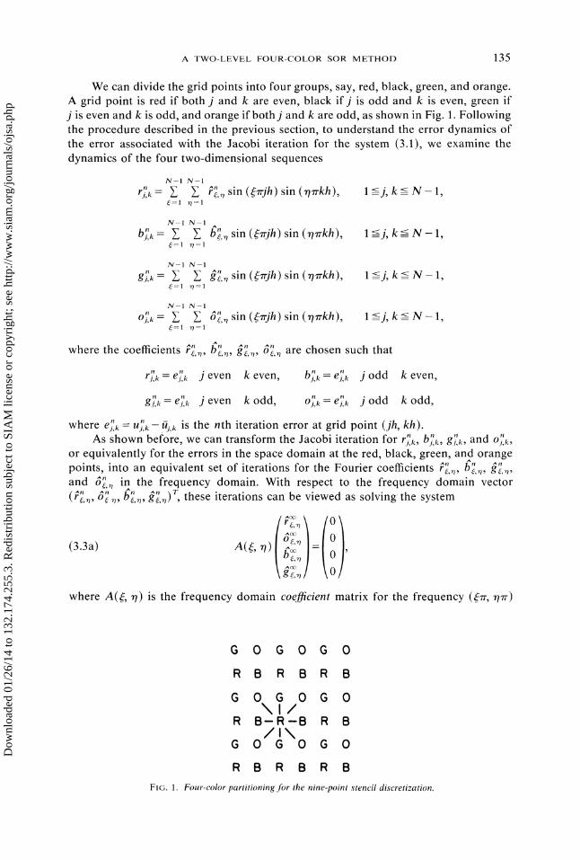
We can divide the grid points into four groups, say, red, black, green, and orange.A grid point is red if both j and k are even, black if j is odd and k is even, green ifj is even and k is odd, and orange if both j and k are odd, as shown in Fig. 1. Followingthe procedure described in the previous section, to understand the error dynamics ofthe error associated with the Jacobi iteration for the system (3.1), we examine thedynamics of the four two-dimensional sequences

N-1 N-1

rjn, k 2 E -,, sin (rjh) sin (rkh), l<=j,k<=N-1,

N-I N-1

b,, sin (rjh) sin (rlrkh),=] ,=

l<-j,k<-N-1,

N-1 N-1

gj, 2 E v.,g sin ((rjh) sin (r/rkh)=1

l<=j,k<=N-1,

N-1 N-I

o.i.k ,, sin (rjh) sin (rrkh),=1 =

l<=j,k<=N-1,

where the coefficients ,,, b.....,,, ge,,, o,, are chosen such that

rj, k elk j even k even, bj,k-- elk j odd k even,

gj,= e,i,k j even kodd, oj,= e,, j odd k odd,

where ej,k U.i,- ffi, k is the nth iteration error at grid point (jh, kh).As shown before, we can transform the Jacobi iteration for ?’.j,k, bj, k, gj,,, and o.i,k,

or equivalently for the errors in the space domain at the red, black, green, and orange"npoints, into an equivalent set of iterations for the Fourier coefficients r,, b,,

and t3, in the frequency domain. With respect to the frequency domain vectorn "nr,, 0 . , , ge, )r, these iterations can be viewed as solving the system

(3.3a) A(, r/

where A(sC, r/) is the frequency domain coefficient matrix for the frequency ((, r/Tr)

6 0 6 0 6 0

R B R B R B

G 0 G 0 G 0\1/

R B-R-B R B/1\

G 0 G 0 G 0

R B R B R BFIG. 1. Four-color partitioning for the nine-point stencil discretization.

Dow

nloa

ded

01/2

6/14

to 1

32.1

74.2

55.3

. Red

istr

ibut

ion

subj

ect t

o SI

AM

lice

nse

or c

opyr

ight

; see

http

://w

ww

.sia

m.o

rg/jo

urna

ls/o

jsa.

php

136 C.-C. J. KUO AND B. C. LEVY

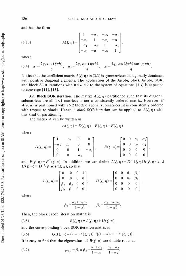
and has the form

(3.3b) A((, rt)

where

J0/3 --0/1 --0/2

0/3 1 --0/2 --0/1

0/2 --0/1 3

2q cos ((Trh) 2q2 cos (r/Trh)(3.4) 0/= 0/2--- 0/3--

4q3 cos ((’h) cos (’h)q q q

Notice that the coefficient matrix A(sc, r/) in (3.3) is symmetric and diagonally dominantwith positive diagonal elements. The application of the Jacobi, block Jacobi, SOR,and block SOR iterations with 0<w <2 to the system of equations (3.3) is expectedto converge 11 ], 13].

3.2. Block SOR iteration. The matrix A(c, r/) partitioned such that its diagonalsubmatrices are all matrices is not a consistently ordered matrix. However, ifA(:, r) is partitioned with 2 2 block diagonal submatrices, it is consistently orderedwith respect to blocks. Hence, a block SOR iteration can be applied to A((, r/) withthis kind of partitioning.

The matrix A can be written as

where

A((, r/)= D(:, r/)- E(:, r/)- F(:,

D(sC, r/)=

-a 0 0 0 0 0/1

.1 0 0E(s:,)__.

0 0 a

0 1 -[e3 0 0 0

0 -a3 0 0 0

and F(:, r/)= Er( r/). In addition, we can define L(, 7)= D-(, n)E(, q) andU(, r/)-= D-’(:, r/)F(s, /), so that

0 0 0 3

0 0 0 0U(:, n)L(,r/)=

fi, fi2 0 0

/3: /3 0 0

0 0 1 ]’20 0 /20 0 0 0

00 0 0

where

1 q- 0/20/3/2

1--0/3

Then, the block Jacobi iteration matrix is

B((, r/)= L(:, r/)+ U(:, r/),

and the corresponding block SOR iteration matrix is

(3.6) G,o(, r/) (I- wL(, r/))-’{(1 o9)I+ wU(ff,

It is easy to find that the eigenvalues of B(sc, r) are double roots at

(3.7) /d,,rt / q-/20/1 + 0/2 0/1 0/2

1--0/3 1+0/3

Dow

nloa

ded

01/2

6/14

to 1

32.1

74.2

55.3

. Red

istr

ibut

ion

subj

ect t

o SI

AM

lice

nse

or c

opyr

ight

; see

http

://w

ww

.sia

m.o

rg/jo

urna

ls/o

jsa.

php


Note that the eigenvalue (l-k-2)/(l--3) at the frequency (r, r) has the samevalue as the eigenvalue (cl- c2)/(1 + c3) at the frequency (r, (N- 7)r) and, hence,we only have to consider the eigenvalues ( + 2)/(1- 3), , 1, 2,..., N-1.

The eigenvalues e, of the Jacobi iteration matrix B(, ) and the eigenvaluesAe, of the SOR iteration matrix G(, ) are related by

,,n"

Hence, if we proceed as in the one-dimensional case, except for a change of subscriptfrom the one-dimensional index to the two-dimensional index (, ), we find that

A,,2

where w -4( 1)

and the spectral radius of G((, ) is

if>O,P,n

w,n- if0.

The above quantity is minimized for all and by choosing the following optimalrelaxation parameter

2(3.8) w* /2 where max= max ,,

l+[1--mx] l,nu-

and the spectral radius of the corresponding SOR matrix is

p*=w*-l.

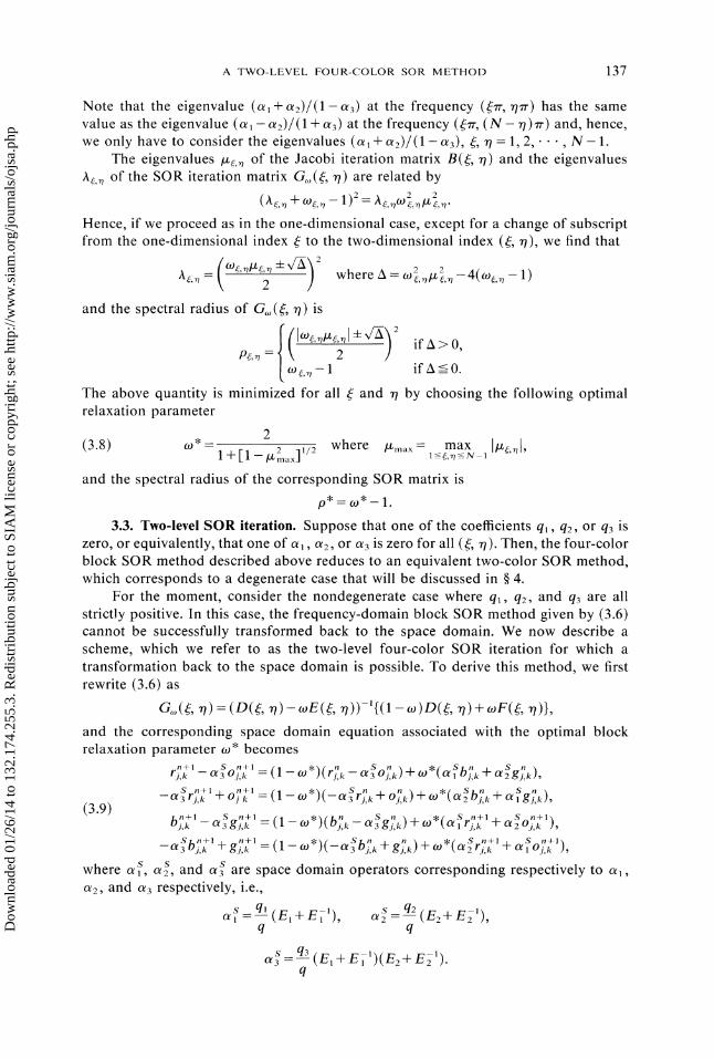
3.3. Two-level SOR iteration. Suppose that one of the coefficients q, qz, or q3 iszero, or equivalently, that one of , 2, or 3 is zero for all (, ). Then, the four-colorblock SOR method described above reduces to an equivalent two-color SOR method,which corresponds to a degenerate case that will be discussed in 4.

For the moment, consider the nondegenerate case where q, q, and q3 are allstrictly positive. In this case, the frequency-domain block SOR method given by (3.6)cannot be successfully transformed back to the space domain. We now describe ascheme, which we refer to as the two-level four-color SOR iteration for which atransformation back to the space domain is possible. To derive this method, we firstrewrite (3.6) as

(, n) (D(, n)-(, n))-’{(1- )D(, n) +(, n)},and the corresponding space domain equation associated with the optimal blockrelaxation parameter w* becomes

n+l n+l S S Sri, k --O.i, =(1-- )(ri,-3og,)+w (bi,k+zg.i,k),

n+l S S-;+o. =(1- (-,+o,)+*(,+,g,),(3.9)

b.i+ s + s , s n+ s +-g., =(-*)(-g,)+ (lr, +o., ),__n+l n+l S ,( S n+l S n+l

.i,k +g.i,k =(1--W*)(--3b,k+gi,k)+W r, +o.i, ),where s s s, , and 3 are space domain operators corresponding respectively to ,2, and respectively, i.e., - s q2

(E2+Es q’(E+Eq q

s q3 -1 -1CI -----(E -1

t- E )(J2 hI" E ).q

Dow

nloa

ded

01/2

6/14

to 1

32.1

74.2

55.3

. Red

istr

ibut

ion

subj

ect t

o SI

AM

lice

nse

or c

opyr

ight

; see

http

://w

ww

.sia

m.o

rg/jo

urna

ls/o

jsa.

php


At the (n + 1)th iteration, the values of the solution at the red and orange points andat the black and green points are coupled together as indicated by the left-hand sideof (3.9).

n+lThe procedure defined by (3.9) is implicit in the sense that r2,-1 and o,k are tobe determined from the first pair of equations and b2",[ and g,- are to be determinedfrom the second pair. We consider the following procedure.

n+lStage I. Solve the first pair of equations of (3.9) for rn,[ and o.j,k by using Msteps of the SOR method using to top.

Stage II. Solve the the second pair of equations of (3.9) for b,j,- and g.i,l byusing M steps of the SOR method using to top.

For convenience, we further decompose each stage into two steps. The formulasfor Stage I are as follows.

ffn+l S S SStep Compute,j.i,k (1-tob)(u.i,k-c3 uj,k)+ to,(c U.i, + o2Uj,k-- h fj, k) at redand orange points.

n+l n+lStep 2. Perform iterations at red and orange points to compute r.i, andn+l 0with ffi, as driving function. Specifically, let vj, u.i,, and for m 0, 1, 2,. , M- 1

perform the following iterations:m+l S -1-- fn+lat red points: v.j, (1 --top)V.j,k -- top(t V.j,k--jj j,k

m+l m+l -1- cn+lat orange points: v.i, (l top)V.j,k _Jr_ top(Ogl)j,k --JJ j,kn+l MFinally, set Uj.k

The formulas for Stage II are as follows.S S n+l S n+lStep 3. Compute ggjn,’=(1--tot)(ULk--O3Uj,k)+tot(O, Uj,k + O2Uj,k -h f.i,) at

black and green points.Step 4. Perform iterations at black and green points to compute b,- and g.,-

with gg, as driving function. Thus, let v..1, U,k, and for rn=0,1,2,...,M-1

perform the following iterations"rn/!at black points: v., (1 --top)V,k + top(aV,k + gg,-)m+l S m+l n+lat green points" Vj, k (1 top) V.i,k + top (a3 Vj, k + gg.i,g ).

n+l MFinally, set u2, v2,k.

Each time we use (3.9), we are carrying out a first level block (or outer) SOR iteration.Each iteration within either Stage I or II is a second level point (or inner) SOR iteration.Usually the number M of inner iterations in Steps 2 and 4 is two (see 5). For theouter iteration defined by the right-hand side of (3.9), we use the block relaxationparameter to* to, and we use the point relaxation parameter top for the inner iterations.

A data-flow diagram that illustrates how grid points exchange values with theirneighboring points at each step of one two-level iteration is shown in Fig. 2. Forsimplicity, only one inner iteration is illustrated in this data-flow diagram.

It is a well-known result that both the block and point SOR iterations applied toa symmetric positive definite matrix converge if and only if their relaxation parametersare between zero and two I11]. Hence, the convergence of the two-level SOR schemecan be achieved by first selecting

(3.10a) 0 < top < 2 M sufficiently large,

where M denotes the total number of point SOR iterations performed at the secondlevel, so that the point SOR iteration converges inside each block SOR iteration. Undercondition (3.10a), a two-level SOR iteration is not different from a single-level blockSOR iteration. Therefore, by imposing the additional constraint,

(3.lOb) O<tob <2,

Dow

nloa

ded

01/2

6/14

to 1

32.1

74.2

55.3

. Red

istr

ibut

ion

subj

ect t

o SI

AM

lice

nse

or c

opyr

ight

; see

http

://w

ww

.sia

m.o

rg/jo

urna

ls/o

jsa.

php


G 0 G 0

R B--,,R--- B

G--O-- G O

R B R B

G 0 G 0

R.--B--- R B

G ---G-- O

R B R B

step step

G 0 G 0 G 0 G 0

R B"’WR"’B R’WB""R B/’,,, /\

G 0 G 0 G 0 G 0

R B R B R B R B

step 2(0) step 4(0)

G 0 G 0 G 0 G 0

R B R B R B R B’,,, / ",,G/OG/ONG o G O/ \

R B R B R B R B

step 2(b) step 4(b)

FIG. 2. Data-flow diagramfor a two-levelfour-color SOR method with computational order {red orangeblack-+ green}. Step 1: first half of a block SOR iteration. Step 2(a) and (b): one-point SOR iteration for redand orange points. Step 3: second half of a block SOR iteration. Step 4(a) and (b): one-point SOR iteration

for black and green points.

the two-level SOR method is guaranteed to converge. In 5, we will discuss how to* and to* to maximize theselect the number M and optimal relaxation parameters top

convergence rate of the two-level SOR method.

3.4. Rederivation of Adams et al.’s nine-point SOR results. It is possible to derivethe SOR results of Adams, LeVeque, and Young [2] directly from the frequency domainmatrix equation (3.3). To do so, rewrite the coefficient matrix A(:, 7) as

a(, 7) =/(sc, ) -/ (s, n) (sc,where

1 0 0 0 0 a3 a]

/(sc,7) =I: 0 1 0 0 /(s:,7): 0 0 a2 a,

0 0 1 0

0 0 0 1 0 0

Dow

nloa

ded

01/2

6/14

to 1

32.1

74.2

55.3

. Red

istr

ibut

ion

subj

ect t

o SI

AM

lice

nse

or c

opyr

ight

; see

http

://w

ww

.sia

m.o

rg/jo

urna

ls/o

jsa.

php


and /(:, rt)=/r(:, r). In the frequency domain, we can then consider an SORiteration of the form

(3.11)

In the space domain, (3.11) corresponds to Adams et al.’s SOR method with RO/B/Gordering, which can be written as

S S Sr:[’ (1 -w)r, + w a bj, + a z g, + 0j, k

n+l (S S n+l

(3.12)oj, =(1-w)o2,+w gi,+abj,+a3ri, ),

bj;, _o)b, + o(s n+l

n+l S n+l S n+l S n+l).g,k =(1--w)g,k+W(lO,k +2rJ, +3bj,k

If , is an eigenvalue of (, ) we have

(3.13)

which is a quartic equation of the variable e,. In [2], Adams et al. derived a quarticequation in terms of the variable Y ([e,n)/2 and showed that if

(3.14a) 4where c, 1 N N 4 are functions of w, (, and is the quartic equation for the frequency(, ), then

(3.14b) T4- C1T + C2T2- C3T + C4 0

is the quartic equation for the frequency (, (N-)). It turns out that the equation(3.13) obtained by our approach is equal to

(T4+ C T + CT + C3T + C4)(T4- CT + C2T2- C3T2- C3T + C4) 0.

In other words, (3.13) and (3.14) contain the same amount of information. From (3.13)or (3.14), the optimal relaxation parameter w* has to be selected so that the maximumvalue of p[O(, )] is minimized over all and . For the details of this procedure,we refer to [2].

The major advantage of deriving SOR methods directly from the frequency domaincoefficient matrix A(, ) is that this procedure does not require the knowledge of theeigenvectors of the SOR iteration matrices such as G((, ) in (3.6) and G(, ) in(3.11) for the determination ofthe optimal relaxation parameters and the correspondingspectral radii. We only have to know the eigenvectors associated with the scalaroperators , , and that describe the coupling between grid points of differentcolors. Consequently, the derivation is usually simpler. In addition, if the frequencydomain coefficient matrix is block consistently ordered, the standard SOR theory canbe applied separately at the block and point levels as shown above, and the determina-tion of the optimal block and point relaxation parameters becomes straightforward.

However, our Fourier/Fourier approach has several limitations. Sometimes, eigen-vectors provide valuable information for understanding the convergence property ofan SOR iteration scheme. For example, for the SOR method (3.12), it was found thatthe eigenvector associated with the spectral radius is highly oscillatory. Therefore, theobserved convergence rate for a test problem with a smooth initial error is faster thanthe predicted convergence rate [2]. Since the eigenvectors for the SOR iteration matrixcannot be found by our approach, this phenomenon cannot be appropriately explained.In addition, our approach does not apply to the SOR method with natural ordering.

Dow

nloa

ded

01/2

6/14

to 1

32.1

74.2

55.3

. Red

istr

ibut

ion

subj

ect t

o SI

AM

lice

nse

or c

opyr

ight

; see

http

://w

ww

.sia

m.o

rg/jo

urna

ls/o

jsa.

php


G 0 R B G 0

R B G 0 R B

G 0 R B G 0

R B G 0 R B

G 0 R B G 0

R B G 0 R B

FIG. 3. Another four-color partitioning scheme.

Even for different coloring schemes such as the one shown in Figure 3, for which wehave

s= _E2_+_ E_( s= q2 -01 -[qlE+q3(E E)], a --(E2+E2 ),q q

s 1_

E2+ EE-0l =-[q,E, + q3(E, )],q

and where (3.1) can be rewritten in terms of this choice of 01s, 012,s and 013,S it.is notclear whether a frequency domain equation exists corresponding to (3.3). The difficultyarises because sin ((rjh)sin (rt’kh) is no longer an eigenvector of the operators 01Sl

s s s andand 013. In fact, the results of our paper rely exclusively on the fact that 011, 012,s

013 admit sin (rjh) sin (rtrkh) as a common set of eigenvectors, and this requirementis probably the most serious limitation of our approach. Note, however, that thecoloring scheme of Fig. 3 is asymmetric and is therefore less natural than the oneconsidered in this paper.

4. Degenerate case: Five-point stencils. In this section, we show that the traditionalsingle-level two-color SOR method for a five-point stencil is in fact a degenerate caseof the general two-level four-color $OR method. The following discussion also givesus more insight into the two-level SOR algorithm.

4.1. Standard five-point stencil. The standard five-point stencil discretization ofthe Poisson equation is

h(U.j+l,k + U.j-l,k + U.j,k+l + U.i,k-1- 4Ui,k) =,,

which is a special case of (3.1) with

q=l, q2 1,

Hence, we have

q3 =0, q =4.

cos (rh) cos (ncrh)011 012--’-

2 2013 0,

and

S E2 + E-12012

4

Dow

nloa

ded

01/2

6/14

to 1

32.1

74.2

55.3

. Red

istr

ibut

ion

subj

ect t

o SI

AM

lice

nse

or c

opyr

ight

; see

http

://w

ww

.sia

m.o

rg/jo

urna

ls/o

jsa.

php


* --0 from (2.8). It is easy to check that the second-levelFor this case, we know that w,point SOR iteration becomes trivial and that only the first-level block SOR iterationis necessary, which is identical to the traditional red/black SOR method with thefollowing optimal relaxation parameter

2(4.1) co* cob*

1 +[1 --COS2 (7rh)]1/2

2- 27rh.

4.2. Rotated five-point stencil. Another five-point stencil discretization of thePoisson equation is [5]

1

2hUj+ l,k+ -1

t"U.j+ l,k_

I- Uj_ l,k+ -41-Uj_l,k_ -4 Uj,k f.j,k

which is also a special case of (3.1) with

ql=0, q2=0, q3=, q=2.

Consequently, we find that

0/1--0, 0/2---0 0/3 COS (:rh) cos (rtrh),

and

S Sc,=0, c2s=0, c3=(El + E-I)(E2+E)

It turns out that Ob* 1, and in this case the first-level block SOR iteration becomestrivial. Only the second-level point SOR iteration is necessary, which can be written as

n+luj,, =(1-w*)u.,+oo*(0/uj,,-h ,,) (j, k) redorblack,

u.j,k =(1-w uj,,+oo 0/3u.i,, -h ,) (j,k) orangeorgreen,

where

2(4.2) w*=w l+[l_cos4(vrh)]l/2-2-2x/Trh.

By comparing (4.1) and (4.2), we find that the only difference between the standardand rotated five-point stencil discretizations is that the mesh size is h in the first caseand x/h in the second case. Therefore, the optimal relaxation parameter w* andspectral radius p*= w*-1 have to be adjusted accordingly. Note, however, that theabove observation depends on the isotropy of the Poisson equation, since the standardand rotated five-point stencils give rise to different discretizations in the anisotropic case.

5. Convergence rate analysis. In this section, we show how to select the optimal* for the two-level four-color SOR method describedrelaxation parameters w* and w,

in 3, and we analyze the convergence rate of the resulting method when it is appliedto (3.1) with nondegenerate coefficients, i.e., for

q ;> O, q2 > O, q3 > O.

5.1. Determination of optimal two-level relaxation parameters. First, let us concen-trate on the second-level point iteration. In order to determine the optimal relaxationparameter, we need to find the spectral radius of the point Jacobi iteration, given by

/xp.... max 10/31 =4q3cOS2 (7rh)4q--23(1-vr2h2),

1_-<_:,,_-< N-1 q q

Dow

nloa

ded

01/2

6/14

to 1

32.1

74.2

55.3

. Red

istr

ibut

ion

subj

ect t

o SI

AM

lice

nse

or c

opyr

ight

; see

http

://w

ww

.sia

m.o

rg/jo

urna

ls/o

jsa.

php


where the maximum value of Icl occurs for (:, r/) (1, 1). and (N 1, N 1). Sincethe spectral radius of the point Jacobi iteration is bounded by the constant 4q3/q,which is less than one, even a simple point Jacobi relaxation converges reasonablyfast. Nevertheless, this can be further improved by a point SOR iteration using thefollowing optimal relaxation parameter:

*=2/1+[1 (4q3)2COS4q (h)] 1/2 1(2)4

with spectral radius

(5.2)

* 0.01. Since theFor a typical example, we have q3 1 and q 20 (see 6) so that pperror can be damped approximately at the rate 10-2M, where M is the number ofsecond-level iterations, only two- or three-point SOR iterations inside each block SORiteration are necessary. The fact that the second-level point SOR iteration requiresonly a constant number M of steps to converge, where M is usually two or three,plays a crucial role in our analysis of the convergence rate of the two-level SOR method.

,By using this observation, it will be shown below that the convergence rate of thetwo-level SOR scheme is similar to that of the standard SOR method for a five-pointstencil, or of the nine-point SOR scheme discussed in [2].

Next, we examine the first-level block iteration. The spectral radius of the blockJacobi iteration matrix (3.5) is given by

].g b, max1<,/ N-1

2(ql + q2) cos (h)q 4q3 cos2 (rh)

which occurs at (, r/) (1, 1), (1, N 1), (N 1, 1), and (N 1, N 1). By using thefact that q 2ql + 2q2 + 4q3, we can simplify/x b, as

/.L b,(1__ 4q3 2(q 4q3) cos(’nh)

1- + -n hq-4q3cos2(Trh) \2 q-4q3/

Hence, the optimal relaxation parameter for the block SOR iteration is

2

7, ( 8q3 ) 1/2

(5.3) C0*=1 +(1 --/X’,max) 1/22-2

1 +q --4q3

rh,

and the spectral radius is

8q ’ 1/2

(5.4) Oh* rob*- 1 -2 1 + rrh.q --4q3/

Therefore, if q3 1 and q 20, then Pb* 1- v/-rh.Since for a fixed point, the two-level SOR method divides neighboring points into

two groups and operates on one group at the block iteration level and on the othergroup at the point iteration level, and since each block SOR iteration at the first levelrequires M point SOR iterations at the second level, it is convenient to define theeffective number of iterations for one two-level SOR iteration as

(5.5) netr=wpM -t- Wbw, + wp

Dow

nloa

ded

01/2

6/14

to 1

32.1

74.2

55.3

. Red

istr

ibut

ion

subj

ect t

o SI

AM

lice

nse

or c

opyr

ight

; see

http

://w

ww

.sia

m.o

rg/jo

urna

ls/o

jsa.

php


where wb and wp represent the amount of work required per block and per pointiteration respectively. The number he, measures approximately the computationalburden of one full two-level SOR iteration in terms of equivalent nine-point Jacobiiterations.

If the point SOR iteration converges in M iterations, the convergence rate of thetwo-level SOR method is then only determined by that of the block SOR iteration.Therefore, we can define the effective spectral radius of the two-level SOR iteration as

(5.6)

which is used to measure the average smoothing rate per effective iteration of thetwo-level SOR scheme.

For the above example, since the amount of computational work for each blockand point SOR iteration is the same, we have wp wb, so that

M+I 2near- p 1 x/-zrh.

2 M+I

When M 2, we find therefore that

3(5.7) net Peg 1-1.63h.

2

The above effective spectral radius *pe, should be compared with the spectral radiuspg* 1-1.79zrh obtained for the nine-point SOR method discussed in [2]. In the nextsection, we will present a two-level SOR method with a different computationl orderingfor which the effective spectral radius is *pn 2.26zrh.

We see from the above comparison that the two-level SOR method and thenine-point SOR procedure of [2] have very similar convergence rates. The maindifference is of course that the method of [2] is a single-level method that uses onlyone relaxation parameter co*. In addition, its convergence rate analysis requires thestudy of the solution of a quartic equation, and does not yield closed-form relationsbetween p*, w* and the spectral radius /z of the nine-point Jacobi iteration matrix.By comparison, the approach we used above to study the convergence of the two-levelSOR method relies on the standard SOR theory, and provides closed-form relations

and and between p* w b*, and /J’b,between pp*, wp, /Xp,Finally, note that the amount of work required by each effective iteration for the

nine-point stencil case is about twice as large as for a standard five-point SOR iteration.Thus, to compare the convergence rate of the two-level SOR method with that of thestandard five-point SOR scheme, we must compare Pe* with the spectral radius(p*) 1-47rh corresponding to two five-point SOR iterations. This comparison seemsto indicate that the five-point SOR iteration converges faster than the two-level SORmethod, or the nine-point SOR method discussed in [2]. However, the nine-pointstencil discretization is more accurate than the corresponding five-point stencil discretiz-ation. Thus, for the same accuracy, we can select h larger for the nine-point stencildiscretization so that in actuality the two-level or single-level nine-point SOR methodsmay converge faster than the standard five-point SOR method.

5.2. Computational order. In the above discussion, we have used a particularcomputational order, i.e., {red- orange- blackgreen}. Now, let us consider othercomputational orderings. Although there exist 4! 24 different ways to permute thecomputational order for these four colors, they only result in three different two-levelSOR iteration schemes. By interchanging the relative positions of c, ce, and c3 in

Dow

nloa

ded

01/2

6/14

to 1

32.1

74.2

55.3

. Red

istr

ibut

ion

subj

ect t

o SI

AM

lice

nse

or c

opyr

ight

; see

http

://w

ww

.sia

m.o

rg/jo

urna

ls/o

jsa.

php


the matrix A(, r/), we can obtain only six different matrices, each of which correspondsto four different computational orderings. Furthermore, we can divide these six matricesinto three classes"

It is easy to see that the same two-level SOR method applies to matrices withinthe same class. Although the discussion in 5.1 applies only to Class 3 matrices, wecan use a similar approach to obtain optimal block and point relaxation parametersand spectral radii for a two-level SOR method for matrices of Classes 1 and 2. ForClass 1 matrices, we find

*-1+ *

(5.9) (’Ok* 2__ 2 (q +4q3)1/2 (q 2q]h, p1-2 q+4q]

q-2q]

1/2

rrh

and for Class 2 matrices, we need only to replace q by q2 in the above expressions.The data-flow diagram for the computational order {red - black - green - orange},

which corresponds to a two-level SOR method applied to Class matrices, is shownin Fig. 4. Let us analyze the convergence rate for this two-level SOR iteration. FromFig. 4, it is easy to see that Wp Wb. Therefore, from (5.5) and (5.6), we have

3+M , 4/(3+M)llett JOelt (p b

g

4

Consider now the typical example where q q2 =4 and q3--= 1. By using (5.8) and(5.9), we find that the spectral radius of the point SOR iteration becomes larger, butthe spectral radius of the block SOR iteration becomes smaller, i.e.,

pp* 4 x 10-2,

Therefore, the effective spectral radius can be expressed as

4* x/-gTrh./gear

M+3

This gives

(5.10) * 1-2.267rhPelf ifM =2, */gett 1.89rrh if M=3.

Dow

nloa

ded

01/2

6/14

to 1

32.1

74.2

55.3

. Red

istr

ibut

ion

subj

ect t

o SI

AM

lice

nse

or c

opyr

ight

; see

http

://w

ww

.sia

m.o

rg/jo

urna

ls/o

jsa.

php


By comparing (5.7) and (5.10), we observe that the performance of a two-level SORiteration applied to Class or Class 2 matrices is in fact better for this specific example.

6. Numerical examples. We consider the system of equations obtained from anine-point stencil discretization of the Poisson equation, i.e.,

1

6h 2 {4(u.j+ ,k + U.i-,,k) + 4(U.j,k+l +(6.1)

j,k=l,2," ", N-l,

with zero boundary conditions and h 1/N 1/20. In this case, q q2 4, and q3 1.Since in this example the performance of the two-level SOR method for matrices

A(, 7) of Classes 1 and 2 is the same, we compare only the following two computationalorders:

order (a): {red- orange- blackgreen},order (b): {red - blackgreen - orange}.

The computational orders (a) and (b) are obtained by applying the two-level SORiteration to matrices A(, rt) belonging, respectively, to Classes 3 and 1. Their spectralradii and optimal relaxation parameters for the block SOR and point SOR iterationsare summarized in Table 1.

TABLE

order w* p* w p

(a) 1.679931 0.679931 1.009702 0.009702

(b) 1.640105 0.640105 1.042400 0.042400

We use the following two test problems:Example 1. The driving function is e5x [2x(x 1) + y(y 1)(25x- 5x 8)] and

the true solution is e5x x(x-1)y(y-1). In this case, the solution is a smooth functionwith a wideband two-dimensional Fourier spectrum concentrated in the region whereand r/ are small.Example 2. The driving function is -74n- sin (5 n-x) sin (7ry) and the true solution

is sin (5n-x)sin (7ry). This corresponds to the case when the solution is a rapidlyoscillatory function containing a single Fourier component at (, r/)= (5, 7).

The computed results are shown in Figs. 5 and 6, where we plot the maximumerror at each iteration as a function of the number of block SOR iterations. Each curveis parametrized by the number M of point SOR iterations we used. It is almostimpossible to distinguish the curves with M 2, 3, 4 for computational order (a) inboth examples. Hence, it is reasonable to choose M =2 in this case. When thecomputational order (b) is applied to the first example, where the solution containslow frequency components, the curve for M 3 is slightly better than for M 2.Nevertheless, the difference is very small. For the second example, the curves withM 2, 3, 4 are in fact not distinguishable. Thus, for computational order (b), it is stillpreferable to choose M 2, since fewer computations are required.

To demonstrate the convergence rate of the two-level SOR method, we chooseanother test problem with zero driving function and boundary conditions. This is infact a homogeneous Laplace equation and its solution is zero. Two initial guesses areconsidered: (1) a smooth function, which is chosen to be x(x-1)y(y-1); and (2) a

Dow

nloa

ded

01/2

6/14

to 1

32.1

74.2

55.3

. Red

istr

ibut

ion

subj

ect t

o SI

AM

lice

nse

or c

opyr

ight

; see

http

://w

ww

.sia

m.o

rg/jo

urna

ls/o

jsa.

php


G O G O G

G O--G 0 G

R B R B R

0 G 0

B R

B

step step

G 0 G 0 G 0 G 0

R B---R----B R B R B

G O G O G O’--G---O

R B R B R B R B

step 2(0) step 4(0)

G O G O G O G O

R--,.B--R B R B R B

G O G O G---O---G O

R B R B R B R B

step 2(b) step 4(b)FIG. 4. Data-flow diagramfor a two-levelfour-color SOR method with computational order {red black

green- orange}. Step 1: first half of a block SOR iteration. Step 2(a) and (b): one-point SOR iteration forred and black points. Step 3: second.halfofa block SOR iteration. Step 4(a) and (b): one-point SOR iteration

for orange and green points.

2.5

2

IVI=I----M = 2,3,4

10 20 50 40()

00

M=I2

10 20 50 40(b)

FIG. 5. Computer simulation results for Example with computational orders (a) {red orange blackgreen}; and (b) {red blackgreen orange}. The x-axis is the number offirst-level block iterations and they-axis is the maximum error at each iteration.

Dow

nloa

ded

01/2

6/14

to 1

32.1

74.2

55.3

. Red

istr

ibut

ion

subj

ect t

o SI

AM

lice

nse

or c

opyr

ight

; see

http

://w

ww

.sia

m.o

rg/jo

urna

ls/o

jsa.

php


.0

0.8

0.

0.4 M :2,5,4

0.2

00 iO 20 30 40

1.0

0.8

0.6

0.4

0.2

0

(o)

10 20 30 40(b)

FIG. 6. Computer simulation results for Example 2 with computational orders (a) {red orange blackgreen}; and (b) {red black green orange}. The x-axis is the number offirst-level block iterations and they-axis is the maximum error at each iteration.

random two-dimensional sequence. In Fig. 7, we plot the two-norm of the error versusthe effective number (neff) of iterations for the above two computational orders andM 2. The results show that the two-level SOR method with computational order (b)is better than that with order (a) and that the convergence rate of the two-level SORmethod is not sensitive to the smoothness of the initial errors. Since the problemwith initial guess x(x-1)y(y-1) was also used to demonstrate the convergence rateof Adams et al.’s SOR method in [2], we are able to compare the convergence ratesof our method with theirs for this test problem. It turns out that these two methodshave very similar convergence rates.

7. Conclusions and generalizations. In this paper, we have transformed the systemof equations for a discretized elliptic PDE from the space domain to the frequencydomain in order to interpret the SOR method from a new viewpoint. This newformulation has helped us to design a two-level SOR method with optimal block andpoint relaxation parameters. The resulting two-level four-color SOR method for thenine-point stencil discretization of the Poisson equation was shown to be efficient withspectral radius 1- Crh, and numerical examples confirm our analysis.

Dow

nloa

ded

01/2

6/14

to 1

32.1

74.2

55.3

. Red

istr

ibut

ion

subj

ect t

o SI

AM

lice

nse

or c

opyr

ight

; see

http

://w

ww

.sia

m.o

rg/jo

urna

ls/o

jsa.

php


I0

10-10-210-0-410-

o-’r

0 20 4O 6O 80 100

FIG. 7. Convergence history (two-norm of the error versus the number of effective iterations) for computa-tional orders (a) red orange black green}; and (b) red black green orange} with M 2. Thedriving function is zero and the initial values are (1) x(x-1)y(y-1); and (2) a random sequence.

The constant C of Adams et al.’s SOR method with various orderings and theline SOR method was compared in [2]. The results for the nine-point stencil discretiz-ation can be summarized as follows. The constant C ranges from 1.6 to 2.45 for Adamset al.’s method, C 1.63 or 2.26 for the two-level method, and C 2.82 for the lineSOR method. In practice, when the initial error is smooth, the convergence rate of thetwo-level SOR method is similar to that of Adams et al.’s method. By comparing theconstant C, we see that the line SOR method is slightly faster than both the two-leveland Adams et al.’s methods. However, it should be emphasized that the line SORmethod is less parallelizable since it needs a sequential direct method to solve tridiagonalmatrix equations that describe the coupling between points of each line. Thus, froma parallel processing point of view, the two-level and Adams et al.’s SOR methods aremore attractive.

The two-level SOR iteration method presented here can be generalized easily tohigher-dimensional problems. A three-level eight-color SOR scheme can be describedas follows. Consider a nondegenerate 27-point discretization of the three-dimensionalPoisson equation. Suppose that each grid point is indexed by (j, k, l). We can labelthese points with eight colors depending on whether j, k, and are even or odd.Following a procedure similar to the one used in 3, we transform the discretizedsystem from the space domain to the frequency domain so that in the frequency domainwe obtain a discretization matrix which is block diagonal with 8 8 block matricesalong the diagonal. Each of these blocks describes the coupling of the Fourier com-ponents of the eight colors at a fixed frequency. Since the discretization scheme isnondegenerate, each 8 8 matrix block is full. In order to apply the SOR method foreach of these 8 8 matrices, we can block partition them into 4 4 submatrices. Thisresults in a first-level block SOR iteration. However, the first-level block SOR iterationrequires inverting 4 4 full matrices, which can be accomplished by performing severalsecond-level block SOR and third-level point SOR iterations. Note that both thesecond-level block SOR and third-level point SOR iterations require a constant number

Dow

nloa

ded

01/2

6/14

to 1

32.1

74.2

55.3

. Red

istr

ibut

ion

subj

ect t

o SI

AM

lice

nse

or c

opyr

ight

; see

http

://w

ww

.sia

m.o

rg/jo

urna

ls/o

jsa.

php


of steps to converge. The total number of iterations required by the above three-levelSOR method, which is O(1/h), is therefore determined primarily by the convergencerate of the first-level block SOR iteration.

There are many different possible computational orders for the above three-levelSOR procedure. A typical one can be chosen as follows. At the first-level, we candistinguish two big blocks depending on whether (j+ k+ l) is even or odd. At thesecond-level, within each big block, points are further divided into two smaller blocksaccording to whether (j + k) is even or odd. Finally, at the third-level, each color canbe separated from each other.

It is straightforward to generalize the above procedure to obtain an n-dimensionaln-level 2n-color SOR method. Here, we have considered the case where n 2.

Another generalization of interest would be to extend the two-level SOR iterationprocedure described in this paper to PDEs with space-varying coefficients. It is naturalin this context to combine the two-level SOR method discussed here with the localrelaxation procedure developed in [4], [6], and [9]. The main idea ofthe local relaxationmethod can be roughly stated as follows. Each local finite difference equation is viewedas if it were homogeneous over the entire problem domain so that at each point a localrelaxation parameter is determined on the basis of the local coefficients of the PDEand of the boundary conditions for the whole domain. Hence, a two-level localrelaxation method would use the local coefficients and boundary conditions to chooseoptimal local block and point relaxation parameters at each grid point, so that differentgrid points would therefore have different block and point relaxation parameters.

Note that the Fourier/Fourier approach described in this paper depends heavilyon the specific coloring and partitioning scheme we used. The relation existing betweenthe single-level rowwise and multicolor SOR methods for the five-point stencil andthe nine-point stencil cases can be explained by introducing a tilted grid [10], [2].There does not seem to be an easy way to apply the tilted grid concept to obtain atwo-level rowwise SOR method.

Aeknowlelgments. The authors thank Professor Lloyd N. Trefethen for his com-ments at various stages of this work. The authors are also grateful to the referees forseveral valuable suggestions, and in particular for pointing out the rederivation ofAdams et al.’s SOR method presented in 3.4.

REFERENCES

L. ADAMS AND H. F. JORDAN, IS SOR color-blind? SIAM J. Sci. Statist. Comput., 7 (1986), pp. 490-506.

[2] L. ADAMS, R. J. LEVEQUE, AND D. M. YOUNG, Analysis of the SOR iteration for the nine-pointLaplacian, SIAM J. Numer. Anal., 25 (1988), pp. 1156-1180.

[3] L. ADAMS AND J. M. ORTEGA, A multi-color SOR method for parallel computation, ICASE Report,82-9, ICASE-NASA Langley Research Center, Hampton, VA, April 1982.

[4] E. F. BOTTA AND A. E. P. VELI)MAN, On local relaxation methods and their application to convection-

diffusion equations, J. Comput. Phys., 48 (1981), pp. 127-149.[5] G. DAHLQUIST, A. BJORCK, AND N. ANDERSON, Numerical Methods, Prentice-Hall, Englewood

Cliffs, NJ, 1974.[6] L. W. ERHLICH, The Ad-Hoc SOR Method: A Local Relaxation Scheme, in Elliptic Problem Solvers

II, Academic Press, New York, 1984, pp. 257-269.[7] S. P. FRANKEL, Convergence rates of iterative treatments ofpartial differential equations, Math. Tables

Aids Comput., 4 (1950), pp. 65-75.[8] P. R. GARABEDIAN, Estimation of the relaxation factorfor small mesh size, Math. Tables Aids Comput.,

10 (1956), pp. 183-185.[9] C.-C. J. Kuo, B. C. LEVY, AND B. R. Muslcus, A local relaxation method for solving elliptic PDEs

on mesh-connected arrays, SIAM J. Sci. Statist. Comput., 8 (1987), pp. 530-573.

Dow

nloa

ded

01/2

6/14

to 1

32.1

74.2

55.3

. Red

istr

ibut

ion

subj

ect t

o SI

AM

lice

nse

or c

opyr

ight

; see

http

://w

ww

.sia

m.o

rg/jo

urna

ls/o

jsa.

php


[10] R. J. LEVEQUE AND L. N. TREFETHEN, Fourier analysis of the SOR iteration, Numerical AnalysisReport 86-6, Department of Mathematics, Massachusetts Institute of Technology, Cambridge,MA; ICASE Report 86-93 ICASE-NASA Langley Research Center, Hampton, VA, September 1986.

[11] R. S. VARGA, Matrix Iterative Analysis, Prentice-Hall, Englewood Cliffs, NJ, 1962.[12] D. M. YOUNG, Iterative methods for solving partial differential equations of elliptic type, Ph.D. thesis,

Harvard University, Cambridge, MA, 1950.[13] D. M. YOUNG, Iterative Solution of Large Linear Systems, Academic Press, New York, 1971.

Dow

nloa

ded

01/2

6/14

to 1

32.1

74.2

55.3

. Red

istr

ibut

ion

subj

ect t

o SI

AM

lice

nse

or c

opyr

ight

; see

http

://w

ww

.sia

m.o

rg/jo

urna

ls/o

jsa.

php

A Two-Level Four-Color SOR...

Documents

Transcript of A Two-Level Four-Color SOR...