A TWO-COMPONENT RAIN MODEL FOR THE PREDICTION

OF ATTENUATION AND

DIVERSITY IMPROVEMENT

by

Robert K. Crane

Thayer School of EngineeringDartmouth College

Hanover, New Hampshire 03755

February 1982

Prepared for

Environmental Research & Technology, Inc.

Under their Contract NASW-3506

with the

National Aeronautics and Space Administration

Washington, D.C.

https://ntrs.nasa.gov/search.jsp?R=19820025716 2018-09-15T12:24:34+00:00Z

ABSTRACT

A new model was developed to predict attenuation

statistics for a single earth-satellite or terrestrial

propagation path. The model was extended to provide

predictions of the joint occurrences of specified or higher

attenuation values on two closely spaced earth-satellite

paths. The joint statistics provide the information required

to obtain diversity gain or diversity advantage estimates.

The new model is meteorologically based. It was

tested against available earth-satellite beacon observations

and terrestrial path measurements. The model employs the

rain climate region descriptions of the Global rain model.

The rms deviation between the predicted and observed

attenuation values for the terrestrial path data was 35

percent, a result consistent with the expectations of the

Global model when the rain rate distribution for the path

is not used in the calculation. Within the United States

the rms deviation between measurement and prediction was

36 percent but worldwide it was 79 percent.

ACKNOWLEDGEMENT

The author wishes to acknowledge the help of his

daughter, Cindy, in providing some of the pocket

calculator calculations of slant path attenuation

statistics needed to check the computer runs. He also

wishes to acknowledge the help of D. Blood while at

the Environmental Research & Technology, Inc. in the

preparation of the table of coefficients representing the

rain climate zone rate distribution.

11

TABLE OF CONTENTS

Page

1. INTRODUCTION 1

2. THE TWO-COMPONENT MODEL 6

2.1 Point Rain Rate Distribution 8

2.2 Path Averaged Rain Rate 19

2.3 Attenuation on a Terrestrial Path . . 31

2.4 Attenuation on an Earth-Space Path 33

3. COMPARISON BETWEEN PREDICTED AND MEASURED ATTENUATIONVALUES 40

3.1 Terrestrial Path Observations 42

3.2 Earth-Satellite Path Observations 50

3.3 Summary 56

4. PREDICTION OF JOINT ATTENUATION STATISTICS 58

4.1 Joint Statistics Model 58

4.2 Comparison with Measurements 62

5. CONCLUSIONS 69

6. REFERENCES 71

APPENDIX 77

ill

LIST OF ILLUSTRATIONS

Figure Title Page

1 Radar reflectivity map (la) and calculatedattenuation values for a 1.4° elevationangle scan through a New England shower,(lb).Observations made with the MillstoneL-band radar (Crane 1971) 9

2 Revised rain climate zones for thecontinental United States 11

3 Revised rain climate zones for westernEurope 12

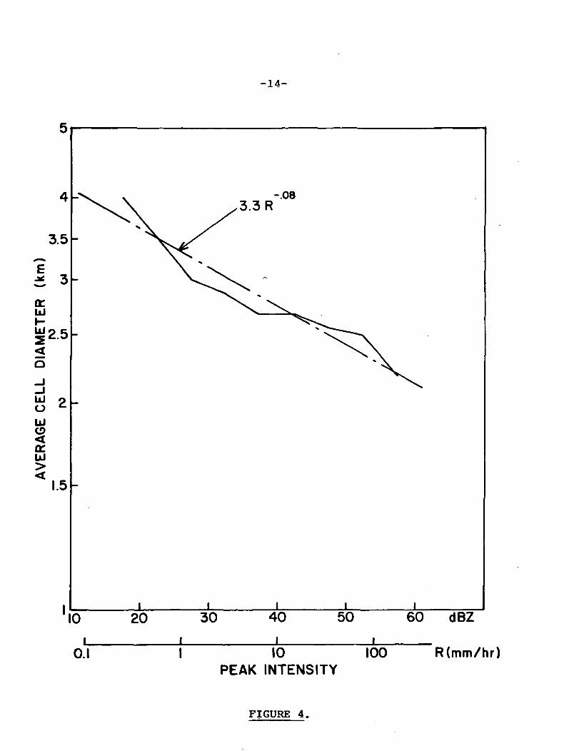
4 Average volume cell diameter as a functionof cell intensity measured in reflectivity(dBz) or rain rate (R) 14

5 Average vertical extent and summit heightfor volume cells observed in Kansas 15

6 Empirical distribution functions for Kansas . 16

7 Areas containing the centroids of volume cellsaffecting a point or a path of length D.Illustrations for circular and square volumecells 24

8 Radar observed debris area vs. rain rate forwestern Kansas 25

9a Path average reduction factor for a 5 kmpath 29

9b Path average reduction factor for a 22.5 kmpath 30

10 Rain height vs. latitude for the Global,CCIR, and Two-Component Models 36

11 Observed and modeled attenuation distributionfunctions for two different path lengths andrain climate regions. Terrestrial pathmeasurements from Fedi (1981) 43

12 Bias and rms deviations for individualterrestrial paths as a function of frequency . 45

iv

LIST OF ILLUSTRATIONS (cont.)

Figure Title Page

13 Bias and rms deviations for individualterrestrial paths as a function ofpath length 46

14 \J vs. the natural logarithm of the ratioof the measured rain rate exceeded 0.01percent of the year to the rain climatezone estimate at the same percentage ...... 47

15 Observed and modeled attenuationdistribution functions for two differentfrequencies on earth-satellite paths.Measured data from Ippolito (1981) 51

16 Bias and rms deviations for individual slantpaths as a function of frequency 53

17 Bias and rms deviations for individual slantpaths as a function of latitude 54

18 Schematic view of the area occupied by thecentroid of a rain region affecting bothslant paths in a diversity system. Theupper figure is for a circular rain area,the lower for a square rain area 60

19 Single site and joint statistics for lowelevation angle measurements at Blacksburg(Towner et al. 1982) 63

20 Single site and joint statistics from theradar simulations reported by Goldhirsh(1981) for 28.6 GHz at an elevation angleof 45° 64

21 Single site and joint statistics for lowelevation angle radiometer measurementsreported by Strickland (1977). The elevationangle at Quebec was 18.5°; at Ontario it was15.5° 65

A TWO-COMPONENT RAIN MODEL FOR THE PREDICTION

OF ATTENUATION AND DIVERSITY IMPROVEMENT

1. INTRODUCTION

Attenuation due to rain has long been recognized as a

major limitation to reliable communication system operation

at frequencies above 10 GHz (e.g. Crane 1971, 1977). The

large fade margins required for satisfactory system

performance at all but the extremely small percentages of

time demanded by many system users are expensive if not

impossible to achieve. One of the methods proposed for the

mitigation of the effects of attenuation on communication

system performance employs space or path diversity (Hogg 1967,

Allnutt 1978, Lin e_t ;al. 1980). Communication is

effected by two or more spatially separated paths with the

expectation that severe attenuation will affect only one

of the paths at a time. Information required for diversity

system design includes the expected attenuation statistics

for a single path and the joint statistics for two (or more)

spatially separated paths simultaneously suffering the same

or higher attenuations. In this paper, a new model is

presented for the prediction of both single and joint path

attenuation statistics for use in system design.

A number of attenuation prediction models are available

for the calculation of attenuation statistics for a single

-2-

path (e.g. Ippolito et al. 1981, Crane 1980, Dutton et al.

1982, Fedi 1981, Goldhirsh 1982, Lin 1977, Persinger et al.

1980). The models are of two general types; one of which

relies on rain gauge or radar--observations to adjust

attenuation statistics observed on one path for prediction

on another path; the other employs meteorological informa-

tion about the intensity and spatial structure of rain to

effect the prediction. Most of the models rely on the

adjustment of attenuation observations. The "Global"

model developed by Crane (1980) and the "Two-Component"

model presented in this paper are examples of the latter

type. Both types of models are necessary. The former tends

to be more accurate for prediction in similar climate

regions, propagation geometries, and within narrow

frequency limits. The latter are required for application

in different climate regions, for different geometries and

over wide frequency limits.

Several models are available for the prediction of the

improvement to be gained by the use of space diversity

(Ippolito e_t al. 1981, Hodge 1976, Goldhirsh 1981). These

are of the former type based either on spaced-path measurements

or on radar simulations of such measurements. The Two-

Component model provides a meteorologically based prediction

method which includes the effects of varying the base line

length and orientation relative to the direction of the

-3-

propagation path, the frequency and the climate

region. The application of the new model has revealed

a wider range of diversity improvement results than predicted

by the earlier models. Available diversity observations are

consistent with the predicted wider range of possible

results.

Both the single path and joint path predictions of the

Two-Component model were compared with available observations

using a modification of the attenuation ratio method

recommended by the CCIR (1982a) and by an equivalent probability

ratio method. A measure of the efficacy of the new model was

obtained by comparison with the results of a similar

measurement and model analysis employing the recently

developed CCIR attenuation prediction procedure (CCIR 1982b;

Fedi 1980).

Terrestrial path data from measurements on 36 paths at

frequencies from 7 to 82 GHz and path lengths from 1.3 to

58 km were used to test the Two-Component (and CCIR) model.

Twenty-nine of the paths were from 10 separate locations in

western Europe. The new Two-Component model predicted the

attenuation values observed in the 0.1 to 0.001 percent of

the year probability range with an rms deviation of 35 percent.

The CCIR model predicted the observed attenuation values with

a 17 percent deviation. These values are within the expected

20 percent rms error for prediction when the rain rate

distribution at a location is known (CCIR model) or the 40

-4-

percent error when only the rain climate region is

specified (Two-Component model; see Crane 1980 or CCIR 1982a).

The observed probability deviations were larger than the

attenuation deviations. The Two-Component model predicted

the probability values at a set of fixed attenuation levels

with a 145 percent rms error while the CCIR model predicted

the probability values with a 49 percent error.

The two models were also compared using available

satellite beacon data. Data from 47 paths were available

for testing the Two-Component model, 17 in the United States,

10 in Europe, and 20 in Japan; data from only 31 of the 47

paths included the point rain rate information required for

the CCIR model, 9 in the United States, 4 in Europe and 18 in

Japan. The beacon measurements were made at latitudes

ranging from 24 to 53°ls7, within a 11.6 to 34.5 GHz frequency

range. The Two-Component model predicted the observed

attenuation values to within an error of 79 percent; the

CCIR model predicted the attenuation values to within 58

percent. The observed probability values were predicted by

the Two-Component model to within 142 percent while the CCIR

model had an error of 166 percent.

Only a limited amount of data were available for

testing the efficacy of the Two-Component model for the

prediction of the joint statistics for space diversity paths.

Low elevation angle satellite beacon observations made at

-5-

Blacksburg (Towner et. al..) at 11.6 GHz compared favorably with

the model predictions. The calculated deviation was less than

6.5 percent for a .baseline of 7.3 km. Comparison with the

radar simulations presented by Goldhirsh (1981) show good

agreement for baselines shorter than 10 km but poor agreement

for longer baselines. Comparison with the radiometer

observations on 18-20 km baselines presented by Strickland

(1978) show model predictions of better than observed diversity

performance. Similarly, the 19 GHz diversity observations

made with the Tampa Triad (Davidson and Tang 1982) show a

progressive increase in prediction error with increasing

baseline. The percent deviation between predicted and observed

attenuation values ranged from 42 percent for an 11 km baseline

to 366 percent for a 20 km baseline.

The new Two-Component model performs well for the pre-

diction of single site attenuation statistics and for

diversity statistics for baselines shorter than about 15 km.

For longer baselines, the prediction errors increase. A

number of model improvements are possible for the longer

baseline situation but additional weather radar observations

are needed first to provide the data required for the

extension of the model.

-6-

2. THE TWO-COMPONENT MODEL

The Two-Component model for the prediction of attenuation

due to rain, separately addresses the contributions of rain

showers and the larger regions of lighter rain fall

surrounding the showers. Some of the earlier models for the

prediction of the statistics of point rainfall rates, such

as the model developed by Rice and Holmberg (1973), recogni2ed

the differences between convective or thundershower rain and

widespread or stratiform rain. Separate roles for thunder-

storm and stratiform rain as different rain types were

maintained through the continued development and use of that

model for attenuation prediction (Button and Dougherty 1973,

Dutton et al. 1982) . The statistical prediction procedures

developed by Misme arid Fimbel (1975) for application to

terrestrial paths and by Misme and Waldteufel(1980) for

application to earth-space paths depended upon the separate

accounting for the effects of rain within cells and within

the wider, lower intensity rain region surrounding the cells.

In their models, a cell was required for the occurrence of

attenuation whether the rain type was classified as

convective or widespread.

Weather radar observations show that rain is always

spatially inhomogeneous with cells occurring in all rainfall

types. Figure la displays the familiar pattern of occurrence

of cells in a convective shower. Figure Ib depicts the

-7-

attenuation values calculated from the radar reflectivity

observations (Figure la) for an azimuth scan through the

shower at an elevation angle of 1.4°. Simultaneous

radiometer observations showed that the attenuation

calculations were correct (Crane 1971). The cell contri-

butions to the attenuation are evident. The reflectivity

peaks - volume cells (Crane: 1979) - are darkened in Figure la,

The darkened areas - volume cells - correspond to three

dimensional regions of a storm with reflectivity values

within 3dB of their local peak values. The horizontal area

of a volume cell is small. The largest of the six volume

cells depicted in Figure .la has a maximum horizontal

dimension of less than 3 km. The more extensive region

of rain debris (within the 20 dBZ contour) surrounding

the volume cells contributes little to the attenuation

when the propagation path traverses a volume cells but

produces all the attenuation for a path which does not

intersect a volume cell. The term "volume cell" is used to

refer to the small volume surrounding a local reflectivity

peak which has reflectivity values greater than one half the

peak value. The term "debris" is used to refer to the larger

region of lighter rain rate surrounding a volume cell. Many

different cell definitions have been used and the modifier -

volume - is employed to specify the quantitative definition

of a radar-observed cell used in this analysis.

The Two-Component model handles the cells - volume

-8-

cells defined by the region within 3dB of local reflectivity

maxima - and the debris independently. All storms contain

volume cells and debris but propagation paths through the

rain do not always intersect a single, isolated volume cell.

For example, Path A in Figure la and Ib does not intersect

a cell and propagation paths through volume cells 1 and 2

or through volume cells 3, 4 and 5 intersect more than one

volume cell. In each of the latter cases the volume cell

at a closer range had a reflectivity value of 5 or more

dB below the peak value of the dominant volume cell and the

effect of the second volume cell could be neglected when

compared with the effect of the dominant volume cell. The

Two-Component model assumes either a single volume cell or

only debris along a path. The model is designed for the

calculation of the probability that a specified attenuation

level Is exceeded. One of the two-components of the rain

process, a volume cell or debris, may produce the attenuation

value. The probability associated with each component is

calculated and the two values are summed to provide the

desired probability estimate.

2,1 Point Rain Rate Distribution

The Global attenuation prediction model (Crane 1980)

provided empirical descriptions of the probability distributions

of point-surface rainfall rate to be expected anywhere within

a rain climate region. A revised version of the Global model

-9-160

160

150

KC

140

130

FIGURE la.

5 dB CONTOURS20 dBZ

10 20 30 40

TRANSVERSE DISTANCE (km)

I I I I I I I I I I I I i I I

275 280 lAZIMUTH (DEC)

I

285

7.8 GHz

15 r

CELL

29

FIGURE lb.

275 280

AZIMUTH (DEG)

285 290

-10-

rain climate region map for the continental United States

is displayed in Figure 2. The major difference between this

and the earlier map is the division of rain climate region B

into 2 sub-regions, Bl and B2 and an adjustment of the contour

region boundaries near the Canadian border to accomodate the

extensive set of rain rate distribution measurements

published by Segel (1979). A revised map for western Europe

is presented in Figure 3. In this case, the map was

redrafted to represent the larger rain rate distribution

data base prepared as a part of the EUROCOP-COST 25/4

Project (Fedi 1979).

The rain climate region boundaries were initially

established using climatological and topographical data.

The data were used to define regions for pooling or

combining available rain rate distribution observations

for estimating a single, best estimate empirical

distribution function for .the region. With the increased

number of rain rate distribution observations now available, some

adjustment in climate region boundaries and in the empirical

distributions is to be expected. The Global model empirical

distribution functions were also extended to span the 0.0001

to 10 percent of the year range where data were available.

The new distribution functions were constrained to produce,

when integrated, the observed average annual rain accumulation

(depth) for each rain climate zone.

-11-

o

CO

UJsUJoc

o

< <I •, —I XX

^J -O CO GJCO O -^ — I**< Or Z HUl ^ . f~ -5 °° _ «* CO Z CL Z

v^ < O _

1 ^ =!^K < CO -J ««^ -« O < °- m o: <

CO

WaD

gU. CO

OUJCO

.0

S -I UJ 03< UJ OD CO

co 3: Q 2 £z h s uj QC^ -J _/ UJ <

< O IT -»$ X O O

« • 4 O<o

-12-

FIGURE 3.

-13-

Results from a three year radar measurement program in

Goodland, Kansas were used to establish the detailed

descriptions of the volume cells and debris regions

required for the attenuation. Average volume cell

parameters were obtained from observations of over 240,000

volume cells gathered from a 25 storm day sample from the 3

year observation set (Crane and Hardy 1980). The average

diameter :'of. a, circular cell with the horizontal area of the

volume cell at the height of peak reflectivity is depicted

in Figure 4, and the average vertical extent is depicted in

Figure 5. Figure 5 also displays the average height of the

highest detected element of a volume cell (summit; see Crane

1979) . The distributions of volume cell area and of volume cell

lifetime were found to be exponential.. (Crane 1979).

The rain occurring over a rain gauge was modeled to

arise from either a volume cell or from the debris

surrounding a volume cell. For the 25 storm days, the

contribution of the volume cells in the 240,000 cell sample

could be calculated based on they area, reflectivity, and

lifetime data for the volume cells and on the surveillence

area and scanning strategy of the radar. The volume cells

produced the rain rate distribution shown in Figure 6. For

display in this figure, the observed occurrence probabilities

for the volume cell component were adjusted by the ratio of

the annual Dl region accumulation to the radar observed

-14-

4

3.5

* 3orUJ

UJp R

5"

o_i_jUJ 'o 'UJt^5

^^j

UJ

< 1.5

10L_

O.I

3.3 R-.08

20 30 40 50 60 dBZ

10PEAK INTENSITY

100 R(mm/hr)

FIGURE 4.

8

-15-

HEIGHTSUMMIT(AGL)

UJ

X 4UJ

o

UJ

THICKNESS

(AGL)

/ GLOBAL MODEL ESIMATE

0°C

10 20 30 40 50PEAK REFLECTIVITY (dBZ)

FIGURE 5.

60 70

-16-

H

VO

« W

A g

(q/tma)

-17-

total accumulation averaged over the surveiHence area of

the radar for the 25 storms. This scaling was necessary

for combining the radar data with the Kansas - region Dl -

distribution function estimate. From this figure, it is

evident that the volume cells contribute little to the

total accumulation but are responsible for most of the

precipitation at rain rates above 30 mm/h and all the

precipitation at rates above 70 mm/h. Calculation showed

that less than 10 percent of the total accumulation was pro-

duced by the volume cells. The rain region surrounding a

70 mm/h volume cell could produce debris with a rate in

excess of 30 mm/h.

A simple approximation to the observed, volume-cell

produced rain rate distribution is an exponential distribution

as illustrated by the volume-cell-model curve in Figure 6.

The portion of the empirical Dl region distribution function

not accounted for by the exponential volume cell component

distribution is attributed to rain debris. The debris distri-

bution function was nearly log-normal over its entire range,

0.001 to 5 percent of the year. Using the rain rate values

in the 0.1 to 10 mm/h range, a log-normal distribution function

was fit to the Dl region curve. The resultant average of the

natural logarithm of the rain rate was -0.2 corresponding to

a rain rate of 0.83 mm/h and the standard deviation was a

factor of 3.1. The average rain rate (predominantly debris;

-18-

calculated by averaging the logarithm of the rain rates)

observed by the radar was 0.8 mm/h and the standard

deviation was a factor of 2.8, nearly identical with the

debris distribution parameters inferred from the Dl

distribution.

The sum of the independent volume cell and debris

distributions, the former exponential and the latter log-

normal, exactly represented the empirical Dl distribution

function as shown in Figure 6. A combination of an exponen-

tial plus a log-normal distribution was found also to fit

precisely the empirical distribution functions for the

other rain climate regions.

The Two-Component model for the empirical rain rate

distribution functions is

P(r >_ R) = Pc(r >_ R) + PD(r _> R) (1)

P (r > R) = P e R/Rc (2)c — c

P D(r>R) = PDH(—— ) (3)

where P(r _> R) is the probability that the observed rain rate,

r, exceeds the specified rain rate, R, (percent). P_(r > R),C """*

P (r > R) are the distribution functions for cells and debrisu *~~

respectively, (percent). r, R are rain rates (mm/h), P is theC

probability of a cell (percent), R is the average cell rainw

-19-

rate (mm/h), n is the normal distribution function, £n is

the natural logarithm, P is the probability of debris

(percent), R is the average rain rate in the debris (mm/h,

calculated from the average of the logarithm of rain rate),

and a is the standard deviation of the logarithm of the

rain rate.

The parameters for the model, P , R , P , R and ac c u u u

for each fo the Global model rain climate zones are listed in

Table I. Table I also includes a listing of the rain rate

expected to be exceeded 0.01 percent of the year.

2.2 Path Averaged Rain Rate

Either a volume cell or the rain debris can produce rain

along a line of rain gauges. The Two-Component model is used

to predict the probability of occurrence of a specified or

higher value of path averaged rain rate by independently

summing the probabilities of a volume cell or of debris causing

the observed path average value.

If a volume cell occurs over, the path, the path integrated

rain rate value is given by:

-£ £ (4)

"o

where i is the observed path integrated value (m2/h), r(£) is

the rain rate profile along the path (mm/h) and D is the

length of the path (Km).

The path integrated rain rate produced by a volume cell

-20-

wPQ

rHO•

o

II

SH PH (~]0 \

sQ \

W D J.(U-P<1>

•gcO ^

15 Q <

|CO «•—•HSHft0)Q Q d?

ft ^^

sW M \.\J ^*.

0) J_

(Ug0

(0

ftrH•H0) O ^Un . °^f-4 ^_x

<Ufi0N

c-H

o inO i n C X J C N V D V D C T i C N O O L n ^r H r H r H C N C N r O ^ T V X ) r H r H < T i C N

^ v^ ro cri in ^i* CTI o i — i i — i cr* or O C N C N r H i - H i - H r H r O ' * ^ ' ! — I V O

r H r H r H r H r H r H r H r H r H r H r H r H

^^ ^^ C^ ^3 fO f O CO 00 ^^ LO ^^ nHC^ C^ CO i1 ^3* 00 ^^ CO CM CO 00 LO

O O O O O O r H r H r H O r H r H

O O O O O O O O O O O O

m c n r - r - c n i n i n m i ^ o o c n c r >

r O C N ^ D C T i O O r ~ C O O r H C O i - l r H

r H i n c n r o ^ m r ^ m c r i o c r i C Nr H r H r H C N C N C N C N r H C N C N r O ^

cr* ^o co cr» ro o r^ o o ^o o oO r H r H r H C N r O r O O C N r H r - ~ ^ DO O O O O O O r H r H O O O

O O O O O O O O O O O O

rH CN rH CN rOW f e f f i

-21-

is approximated by:

RWI = (-g£) (5)

where I is the path integrated rain rate (m2/h), R is the

peak rain rate in the cell (mm/h), W -~Jsis the averageO ™ W

dimension of a volume cell with area S (W - km, S - km2)o c o

and G is an adjustment factor required by the definition of

a volume cell.

The adjustment factor is included to represent the con-

tribution of the debris close to a cell but outside the region

enclosing the -3dB reflectivity value relative to the peak

value (factor of 0.61 in rate rate). The often used GaussianJ

rain cell profile would require a factor of C = 0.68. The

attenuation values plotted in Figure Ib are consistent with

that value for the adjustment factor. The adjustment factor

obtains when the path is much longer than the average volume

cell width. If the path is shorter than W , the actual pathvx

length should be used for the calculation of I and the adjust-

ment factor should be unity.

The rain rate within a volume cell required to produce

the specified path integrated rain rate therefore is modeled by:

R = CI/L (6)o

where L = minimum of D or W (km),c c

1 + .0.7(D - W. )C = 1 + (D - W ) ' (D - V > °

Cx

= 1 ; (D - W ) <_ 0\*r ~™~

-22-

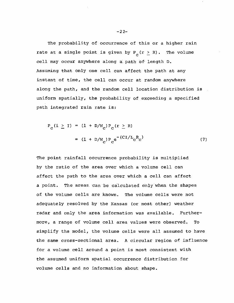
The probability of occurrence of this or a higher rain

rate at a single point is given by P (r >_ R) . The volumeC ~

cell may occur anywhere along a.path of' length D.

Assuming that only one cell can affect the path at any

instant of time, the cell can occur at random anywhere

along the path, and the random cell location distribution is

uniform spatially, the probability of exceeding a specified

path integrated rain rate is:

P (i >!) = (! + D/W )P (r > R)Cx ~™ \~f Cx ~~

(7)

The point rainfall occurrence probability is multiplied

by the ratio of the area over which a volume cell can

affect the path to the area over which a cell can affect

a point. The areas -can be calculated only when the shapes

of the volume cells are known. The volume cells were not

adequately resolved by the Kansas (or most other) weather

radar and only the area information was available. Further-

more, a range of volume cell area values were observed. To

simplify the model, the volume cells were all assumed to have

the same cross-sectional area. A circular region of influence

for a volume cell around a point is most consistent with

the assumed uniform spatial occurrence distribution for

volume cells and no information about shape.

-23-

The average length of a line through a circular

volume cell is given by:

The area of influence of the volume cell about a point is S

and, as shown in Figure 7 the area of influence of a circular

volume cell about a line of length D is:

s. = s (i + JL JL) = s (i + |) (9)c c

Since both the area and shape of the cell is uncertain, it is

sufficient to approximate £ by W =-\/ S yielding the expressionc » c

given in equation (7) . It is noted that a square cell oriented

along the line will produce the same result as equation (9)

with £ = vS = W as illustrated in Figure 7.T C C

The effect of the debris region on the path can only

be calculated if a spatial scale, Wn, is associated with the

rain within the debris. The Kansas radar observations also

provided data on the relationship between average rain rate

and area for isolated echo areas (rain regions completely

within the surveillence area of the radar) . The data were used

to- provide the desired relationship between W^ and the average

rain -rate ..in the debris. The observations are depicted in Figure 8,

The regression 'line: for area vs. rain rate provided the best

-24-

I

= VI w

S. = S (1 + =)

Dp = -±- T,J

I = fs~4 c

S. = S (1 + -)1

FIGURE 7.

10,000-25

I1000

• x

REGRESSION LINE

\

O CENTROID

100 J.0.1

AVERAGE RAIN RATE (itm/h)

FIGURE 8.

10

-26-

fit relationship. The result is:

SD = 8.82 R °'68 (10)

where S is the debris area for rain rate, R, or

WD = 29.7 R"0-34 (11)

where W is the length scale for the debris. As before, the

shape is not well defined and the relationship between the

areas of influence for debris in the vicinity of a point and

a line is calculated as for cells:

PD(r >_ R) = (1 + JL)PD(r _> R) (12)

In the debris, the rain extent may exceed the path

length. The path length used in the calculation of the rain

rate for a specified path integrated rain rate is either the

physical path length or the debris scale length, whichever is

smaller. For a long path:

R = I/WD = IR°'34/29.7 Cmm/h) (13)

1 52therefore R = I /17° Cmm/h)

and WD = I/R = 170I~*52 (Km) (14)

-27-

The model for the calculation of the probability

that a path integrated rain rate, I, is exceeded may be

summarized as

WD = 170 I °*52 (15)

W = Minimum (W /D) (16)

R" = I/WD' (17)

L = 29.7(R")~°'34 (18)

n £n R" - £nR-) n ( - - - -) (19)

W = .J5 = 2.24 (20)C

L = Minimum (17 ,D) (21)C " C

R' = CI/L (22)

1 + 0.7(D - W )

C = ; (° ~ W}> °; C = I otherwise

P (i > I) = (1 + D/W )e R'/Rc (24)C C

The two-component model employs the parameters P , R ,C C

P_, R and cr found by fitting the model distribution function

-28-

to the empirical distribution function for a rain climate region,

the spatial scale parameter W and the coefficient of thec

— 0 34relationship W = 29.7R * deduced from the Kansas radar

observations. The distribution function parameters were allowed

to change from one climate region to the next but the scale

parameters were assumed to apply universally in all climate

regions. The rational for the universality of the scale

parameters is the similarity in scale of the dynamical processes

responsible for the production of rain.

The Two-Component model (2-C Model') was tested by comparison

with path average rain rate measurements made in England (Rain

Climate - C, Jones and Sims 1978) , W. Germany. (.C, Valentin

1977) , Florida (E, Jones and Sims 1978), New Jersey

(D2, Freeny and Grabbe 1969) and Illinois (D2, Jones

and Sims 1978). The path average observations were obtained

in 3 different rain climate regions and each region was

different from the rain climate in the high plains of the

United States (Dl). The measured data were available as path

average reduction factors r = I/RD (Crane 1980). The results of

the modeled vs. measured path average reduction factors are

presented for two path lengths in Figures 9a and 9b. The

results show agreement within the apparent statistical un-

certainty of the observations. The agreement between the measure-

ments and the Two-Component model predictions justified the use of

the universal scale parameter assumption for at least application

WCJ

c/jHA'COKO

H

w

-29-

cQ)O

C4Q

>i WO ~toM «O -Cb -H

fcS OO ^HS fa

>1c

OO

u

•O

(0rHDltj

dP <*P1-4 rHO O

* •

O O

•M 4-1tC Q

0) OT3 -OO O

« CM MU 0U CJ

OOCO

OOIN

OO

OIT)

803

0) 9>4-110 KK K

DC O•H M

in

O

fN

uoj^onpau abeaaAv

-30-

ooCO

oo

Oo

oin

oCN

0)4-110

c••H(3

in

o\

o•

CM

in

uoi^onpaa

-31-

in temperate climate regions.

2.3 Attenuation on a Terrestrial Path

The attenuation on a terrestrial path is given by

-D

•1 kl.r(£)]ada (25)

where a is the attenuation (dB), k, a are coefficients

in the relationship, y = kRa, and y is specific attenuation

(dB/Km). As for path integrated rain rate, the attenuation

within a volume cell is approximated by

A - -a

where A is attenuation (dB) and

C = C (27)d

where C is the adjustment factor needed to estimate thea

additional attenuation outside the volume cell. It is noted

that the equation (27) for C neglects the non-linearity inSi

the relationship between specific attenuation and rain rate.

The effect of the non-linearity is small in comparison with

the expected year-to-year variations in the observed attenuation

or rain rate values at specified probabilities of occurrence.

For a Gaussian volume cell profile, the error in calculating

-32-

attenuation caused by assuming the C vs. C relationship ina.

equation (27) in -3.5% for a = 1.3 and +4.5% for a = 0.75.

The error is therefore less than 5% for the entire range

of values of a for calculations at frequencies between 1 and 100

GHz tCCIR- 1982a) .- By way of contrast, the year-to-year variability

for measured attenuation values at probability values between

0.1 and 0.01% of the year is in excess of 20% (Crane 1980).

The two-component model calculates the probability of

exceeding a specified attenuation value after first estimating

the rain rate in a volume cell or in the debris region re-

quired to produce that value or a higher value of attenuation.

For a volume cell,

R« = (_£ _)1/a (mm/h) (28)

and

P (a > A) = (1 + D/W )e R'/Rc (percent) (29)c —

Similarly, neglecting the effect of the non-linearity on the

relationship between average specific attenuation and average

rain rate within the debris region,

R = C -)Va = C,* )Va R°'34/a (mm/h) (30)

-33-

Therefore,

and

then

and

Finally,

(31)

W = :29.7(a/a~'34) kr.»31/(a-.34)}A{ ;34/Ca-.-34)} (Km) (32)

WD = Minimum (WD/D) (Km) (33)

R" = (A/kWD')1/a (mm/h) (34)

L = 29.1 R«-°-34 (Km) (35)

PD(a > A) = (.1 + D/LD) n (£nR"ff"

£"R») (percent) (36)

P(a >_ A) = Pc(a _> A) + PD(a >_ A) (percent) (37)

is the desired probability that the attenuation value A is

exceeded.

2.4 Attenuation on an Earth-Space Path

Earth-space paths traverse attenuating regions of liquid

-34-

drops - rain - and regions of ice and snow. The ice and snow

contribute little to the attenuation and may be neglected. The

region with rain produces the significant attenuation. The

physical extent of the attenuating region must be estimated be-

fore the volume cell and debris contributions can be calculated.

In contrast to the terrestrial path case, the horizontal pro-

jection of the rain region is not defined by the physical

location of the antennas but is defined by the expected height

to which the rain extends.

The height of the rain region depends upon the dynamical and

physical processes at work in a storm. Some variation in the

height is to be expected, especially in the northern temperate

regions where rain or snow may occur at the ground often within

the same storm. The rain rate distributions are assumed to rep-

resent only periods with rain on the ground and, therefore, a

rain region exists above the ground in all rain climate zones.

Rain usually extends from the ground to a height just be-

low the height of the 0°C isotherm in regions of debris. Radar

observations of .debris are characterized by a bright band or

melting region. The reflectivity values generally vary little on

average below the melting region and therefore, the specific

attenuation can be assumed to be constant from the surface to

the base of the bright band in rain debris (neglecting the

variation of specific attenuation with the physical temperature

of the raindrop).. Radar observations reveal this behavior in

the tropical Atlantic (Houze 1981) in the eastern United

-35-

States (Goldhirsh and Katz 1979) in England (Hall and Goddard

1978), and Japan (Furuhama et al. 1980). Measurements in

wintertime, widespread storms, have on occassion, revealed the

existance of extensive low level regions of raindrop growth

which should effect the average specific attenuation

profiles in the debris regions (Cunningham 1952). The

warm rain'process was initially developed to explain the

occurrence of rain showers in the tropics which do not form

high enough to reach the 0°C isotherm (Mason 1971).

A wide range of seasonal and storm-to-storm

variation can be expected in the height of the rain region in

debris. For the estimation of annual attenuation statistics,

a model must integrate over these effects or use an

effective average height of the rain region which compensates

for the variation. The Global model (Crane 1980) employed

the natural correlation between wintertime, widespread

storms and low rain region heights and intense summertime

convection and higher heights do postulate a variation of

effective height with the probability of occurrence of

specified or higher surface point rain rate values.

The Global model rain height curves are presented in

Figure 10.. They were constructed using observations of the 0°C

isotherm 'height during periods with precipitation and during

periods of excessive precipitation obtained from an analysis

of radiosound data, rain occurrence data, and excessive precipi-

tation data for seven spatially separated sites in the United

-36- oo

o00

oID

0wQ**"**

HQDEHMEH

.O•H

f.

sDOHh

— o

OCN

If)

-LHJI3H NIVH - H

-37-

States (Crane 1980). The data were extrapolated globally

using the observed latitudinal variation of zonally (longitudinal)

averaged temperature profiles. The extrapolations

to latitudes higher than 50° were done by selecting

summertime data. The 1 percent curve corresponded to the

zonally and.seasonally averaged 0°C isotherm height (not

correlated with precipitation). The 0.001 percent curve

corresponded to the 0°C isotherm heights on days with

excessive precipitation events (highest 5 minute averaged

rain rate each year).

The Two-Component model does not employ the correlation

between surface rain rate and rain rate height assumed by the

Global model [and by the recently proposed CCIR model, CCIR,

(1982b)]. It uses an average rain height for debris of all rain

rates and an average rain height for rain in volume cells.

Dynamical reasoning suggests that the more intense volume cells

will be associated with the updraft regions of a storm which

lift liquid particles to higher heights than in the surrounding

debris. The observation that the highest rain rate regions in

a storm are in the volume cells also argues for a higher volume-

cell-rain height than the debris-rain height.

Figure 10 presents the simple latitude variation assumed

for the volume cells and the debris. The equations for this

dependence are:

H = 3.1 - 1.7 sin[2(A - 45°)] (38)

-38-

HD = 2.8 - 1.9 sin[2(A- 45°)] (39)

where HC, HD are the volume cell and debris rain heights

respectively (km) and A is latitude (deg). For reference, the

CCIR model for rain height proposed by Fedi (1981) is also

included in this figure.

The simplest sinusoidal variation was assumed to

represent the latitude dependence. The debris curve was

adjusted to represent the average 0°C isotherm height at low

latitudes and the summer time height at high latitudes. The

volume cell curve was adjusted to lie above the debris curve

with a difference between the two heights roughly equal to the

difference between the heights of the 0°C and -5°C isotherms.

The rain heights HC and H define the vertical

extent of the rain region. The horizontal extent may be

calculated geometrically when the elevation angle to the

satellite is given. Two horizontal distances along the

earth's surface result, one for volume cells, the other for the

debris:

(H - H ) [2 - 2(H - H )/8500] (km)D = - ° ° - (40)

tan 6 + tan0 + (H - H )/8500

where D = DC, DD are calculated for H = H , H , respectively,

6 is elevation angle, H is the height of the earth terminal

and an effective earth's radius of 8500 km is assumed.

The expression for the effective debris and volume cell

distances DD and DC is valid for all elevation angles. It

reduces to the familiar D = (H - H ) /tan 0 at high elevation

angles.

-39-

Th e attenuation values used in the calculation of the

probabilities (P (a > A ) and P (a > A ,) must be reducedC o JJ — o

to the attenuation along a horizontal path,

A = AS cos 0 (41)

where A is the slant path attenuation and A is the reducedo

attenuation.

The reduced attenuation value was obtained using an

assumed constant specific attenuation from the surface to the

rain height. The reduced attenuation value and the effective

distances are used in equations (28) through (37) to calculate

the desired probability values. Note that although the

reduced attenuation values are used in equations (28) and (30)

through (34) , the resultant probabilities given by equation

(29) , (.36) and (37) are for the full slant path attenuation, As.

-40-

3. COMPARISON BETWEEN PREDICTED AND MEASURED ATTENUATIONVALUES

The Two-Component model provides a prediction of the

attenuation statistics for either a terrestrial or an earth-

satellite propagation path. The model is global in nature,

proposed for application anywhere, and does not require

rain gauge or radar statistics from a location for application

at that location. Being global in nature, the model will

produce only one set of attenuation statistics for a path

of a specified length and frequency located anywhere within a

rain climate zone. Observations show that local variations

are to be expected within a rain climate zone and perhaps

between one side and another of a hill within the same town.

The Global model (Crane 1980) included a set of bounds

to be used with the prediction models to describe the expected

location-to-location variation within a region or the

expected year-to-year variation for a single path. A new

variation model is not proposed but the expected variations

predicted by the Global model are summarized for consideration

when comparing measurements and predictions. For a

terrestrial path, the expected rms deviation between model

prediction and measurements was estimated to be 29 percent

at .1 to .01 percent of the year and 36 percent at 1 and

0.001 percent of the year. For earth-satellite paths, the

expected deviations ranged from 32 percent at .1 and 0.01

percent of the year to 39 percent at 1 and 0.001 percent of

the year.

-41-

The Two-Component model was tested against observations

using the procedure proposed by the CCIR (1982a). A test

variable, V, was calculated where

v = £n(A ,/A , ,) (42)measured7 model

and the Ameasured and Amodel values are equiprobable

measured and modeled attenuations. The test variable was

calculated at a set of preselected percentages of the year

spaced by a ratio of 1.78 (i.e. at .0178, .0316, .052, .1,

etc.). The mean and standard deviation of v was calculated

as well as the rms value of v (the deviation). The prediction

method yielding the smallest rms deviation would be judged

the method best matching the observations.

The comparison procedure recommended by the CCIR specified

that v = 0 if the measured and modeled attenuation values

were within 1 dB. That recommendation was not followed for

most of the comparisons presented in this section. Sample

calculations showed that the adoption of this CCIR recommendation

would have made only a slight difference in the final results.

The model was also tested by calculating the rms

deviations in, £, the logarithms of the ratios of measured

to modeled cumulative probability values at specified

attenuation levels. The attenuation values chosen were

1, 2, 3, 5, 7, 10, 15, 20, 25 and 30 dB. The statistics

for both the attenuation deviations, v, and probability

-42-

deviation calculations, £, were reported as percent

deviations,

d = Ce+X - 1) • 100 (43)

where d is the percent deviation and x is the statistic

such as the mean, standard deviation, or rms deviation of

v or £.

3.1 Terrestrial Path Observations

The data base employed for the evaluation of the model

predictions for terrestrial paths was compiled by Fedi

(1981) as a by product of the EUROCOP-COST 25/4 Project

(Fedi 1979). Empirical distribution functions were prepared

to represent the probabilities that specified attenuation

values were exceeded on each of 29 propagation paths in

Western Europe, 3 paths in the United States, and 3 paths in

Japan. Data from an additional path in Brazzaville, Congo

(Moupfouma 1981) were added to the sample to extend the

geographical coverage. One or more years of data were

available for each path. As reported, only attenuation values

in the 0.001 to 0.1 percent of the year range were available.

The mean, standard deviation, and rms deviation values

were calculated for v and £ for each of the paths and

for all the paths. Figure 11 displays sample observations

and predictions for two terrestrial paths for a frequency of

-43-

•ocuT!0)<0UX

0)3r-H(Q

4-> W(D «3 DC C

•HXI(0

(gp)

-4.4-

18 GHz. The test statistics are listed in the figure.

Figure 12 displays the individual path values for the mean

(bias) and rras deviation of v plotted as a function of

carrier frequency and Figure 13 displays the same data

plotted as a function of path length. No obvious

dependences on frequency or path length were evident. A

significant source of deviation between model prediction and

measurement was the difference between the predicted and

observed rain rate. Figure 14 displays this source of

modeling error. In this figure, the ordinate is v, the

average value of v for a path, and the abscissa is the

natural logarithm of the ratio of the measured to modeled

rain rate corresponding to 0.01 percent of the year. From

this figure, it is evident that the modeling uncertainty

is increased by using the rain zone estimates of the rain

rate distributions in place of the reported rain rate

distributions for each location.

The average model bias, v", for all the paths

was -9.8 percent. The average of the '•v values for each of

the paths was -15.7 percent (centroid location in Figure 14).

The difference between the two values arose from the different

weights accorded' to the individual v- values. Up to 9

attenuation ratio values (v values) were possible for a

single path but many paths had fewer due to dynamic range

limitations of the instrumentation.

50

30

-45-

oOSH0. 10

3CO

8 -j«u

§u

S ~30

-50

A

o

2-C

0A AA

*A ^TERRESTRIAL

2-C A Other

A Europe

CCIR • Europe

o Other

80

60

z 40u

Ka

2 20

i

2-C

— -O— — — CCIR

A

O

-*5-10 20 30 40

FREQUENCY (GHz)

FIGURE 12.

80 90

50

30

2tJU(X

e 10

O«KK 02Oi—i

5 -10MC

c.u:

-30a

-50

80

60

UKtJC-

OM

40

20

-4G-

A A

2 - C

CCIR'

2-C

CCIR

A Europe

i: Other

• Europe

o Other

10 20 30 40

PATH LENGTH (km)

FIGURE 13.

50 60 70

c•H4-J<C(X

o;-u(C

C•H

(1)CT

O•

I

I Uc:DOH

CO fc

ICM

•I

in•I

vo•I

-48-

The standard deviation of v was 32.7 percent and the

rms deviation of v was 35.2 percent. The expected rms

deviation for an error free model caused only by location and

yearly variations as predicted by the .Global .model is 30.8

percent, in close agreement with the test statistic.

The average model bias calculated using probability

deviations, £f was -23.2 percent. The standard deviation

and rms deviation of £ were 135 and 145 percent respectively.

These variations are significantly higher than those for v.

No model estimates are currently available for the variation

in £ to be expected.

The evaluation of the utility of the Two-Component

model was completed by comparing the' test: statistics for

this model with the test statistics for the recently proposed

CCIR model (Fedi 1981, CCIR 1982b; see Appendix A for a

description of the model). The mean, standard deviation and

rms deviation values for v were 2.4 percent 16.3 percent, and

16.5 percent respectively.^ The bias, \F, and rms deviation

values for the individual paths are also plotted in Figures

12 and 13. The Two-Component model (2-C) produced 3.7 times

the mean square deviation of the CCIR model. A significant

fraction of the increased mean square deviation is due to the

use of a regional rain rate distribution in place of the

observed distribution as recommended for the CCIR model.

However, the two models performed as expected on the basis

-49-

of the Global model prediction of variation about the

estimated values. When the rain rate distribution is known,

the bias should be small and the rms deviation should be 18

percent. The CCIR model produced a bias, v, 2.4 percent

and an rms deviation of 16.5 percent.

The CCIR model test statistics for probability deviations

were bias, £", equal to 17.7 percent, a standard deviation of

43.6 percent and an rms deviation of 48.8 percent. As for the

attenuation deviations, the CCIR model performed better than

the Two-Component model.

The CCIR model was developed by adjusting the

coefficients to fit western European observations of

attenuation exceeded 0.01. percent of the year. An additional

comparison between the two models was performed using only

the attenuation ratio values at 0.01 percent of the year and

the complete recommendations of the CCIR for model comparison

(v = 0 if the attenuation values differ by less than 1 dB).

For this comparison data were available for 28 western

European paths, 3 for the United States and 3 for Japan.

The rms deviations for the western. European data;, were; 33 . 4

percent and 14.3 percent for the Two-Component and CCIR

models respectively. For the United States, the rms deviations

were 15.7 and 9.8 respectively and for Japan the rms deviations

were 0 and 4.2 percent, respectively. Although the number of

non-European samples was small, the Two-Component model did

better relative to the CCIR model outside Europe than for

-50-

Europe. Overall,, the rms deviations were 30.3 percent and

13.3 percent for the Two-Component model and CCIR model

respectively.

3.2 Ear th-S atellite P at h Ob s e rvati ons

Attenuation observations were assembled from 17 earth-

space paths in the United States, 10 in Europe and 20 in

Japan for which data were available for a year or more. The

data were reported in the CCIR (1982b) at three percentages

of the year or by Ippolito et al. (1981). Examples of

measured and Two-Component model predicted attenuation

distributions for the CTS satellite observations at 11.7 GHz

and from the COMSTAR satellite at 28.6 GHz are presented in

Figure 15. The observations were all made in rain climate

region D2 therefore, the only possible model value differences

are due to the variation in elevation angle and rain height.

Lin et al. (1980) reported that at higher frequencies, the

elevation angle and latitude variations compensate for one

another when viewing the same satellite, a result apparent

at 0.1 to 1;0 percent of the year at 28.6 GHz. 'The additional

variability evident at 11.7 GHz and at the probability range

extremes at 28.6 GHz must be due to local and yearly rain rate

differences and, perhaps, the instrumentation.

The test statistics for v and £ were calculated for each

of the 4-7 earth-satellite paths .The results for the

attenuation ratio statistics were a bias, \J, of -10 percent

-51-

coN

cVO

cc

n a

Ca)oV40)a

•o0)T!(U

Xfc

<B

co

(83C0)4J

10

•§

(UP)

-52-

a standard deviation of 11 percent and an rms deviation of

79 percent. The bias value was nearly identical to the

bias value for application of the model to terrestrial paths

but the variances were a factor of 3.7 larger, 79 vs. 35-

percent rms deviation. The model performance was consistent

with expectations in the United States, the rms deviation«

for v was 35.9 percent when only the paths in the United

States were included, but was poorer than expected for Japan

where the observed rms deviation was 116 percent.

The overall probability ratio statistics for the Two-

Component model were nearly the same for the slant path

and the terrestrial path observations. For the slant path,

the bias, £/ was -13.7 percent, the standard deviation was

139 percent and the rms deviation was 142 percent.

The attenuation ratio statistics for the individual

paths are depicted as a function of frequency in Figure 16

and as a function of latitude (and by implication, elevation

angle and path length) in Figure 17. Again, no obvious

dependences of the model predictions in frequency or on

latitude are evident. The model performs well over the entire

24 to 53° latitude band spanned by the observations. The

high variance values appear to be caused by a limited number

of paths. One such path, Ogasawara, Japan, produced an rms

deviation in v of 195 percent and in £ of 948 percent.

For this path, at an elevation angle of 43°, latitude of 27°

and a frequency of 12.1 GHz, the predicted attenuation to be

LU

ocUJa.

50

30

10

A

O

O

OAOO

-53-

A

AO

SATELLITE

A 2-C

• CCIR

A 2-cn CCIR

DEV

BIAS

ceOo;o;

c;Q.

-10

-30

&A\

CCIR

100

80 2-C

— 60

oLUa.

° 40

20

10 20 30

FREQUENCY (GHz)

FIGURE 16.

40-lh-*-

80 90

-54-

50

30

SATELLITE

2-CC C I R

2-C

C C I R

BIAS

DEV

10CO

tx.oceCi

oI—•

OLU0£CL

-10— CCIR

2-C

°u» A

-30

A

100

80

C 60

CE

o

CCIR

**•IO g

<c>UJo

10 20 30

N. LATITUDE (DEG)

FIGURE 17.

40 50 60 70

-55-

exceeded 0.001 percent of the year was 48 dB, the observed

value was 11 dB. For comparison, this path also produced

large rms deviations from the CCIR model. The rms deviation

values for v and £ were 139 and 1323 percent respectively.

At 0.001 percent of the year, the simplified CCIR model

predicted an attenuation of 39 percent. Other paths at

similar or lower latitudes did not produce similar large

deviations, therefore, the large errors for this path

cannot be attributed to the rain height component of the

model or, from the large discrepency relative to the CCIR

model, in the difference between modeled and measured rain

rate distributions.

The simplified CCIR model (Appendix A) was used to

provide comparison test statistics for the Two-Component

model when applied to earth-satellite paths. The

simplified model used an approximation to the rain height

curve of the Global model for 0.01 percent of the year

(Figure 10) and provided predictions only in the 0.1 to 0.001

percent of the year probability range. Simultaneous rain

rate statistics were available only for 31 of the 47 paths.

The attenuation ratio statistics, ~\> and rms deviation of v

were -12.7 and 57.9 percent respectively. The simplified

CCIR model did not perform as well relative to the Two-

Component model as it did: for terrestrial paths. The mean square

-56-

deviation was only a factor'.of 1.6 smaller than the mean square

deviation for the Two-Component model even though the measured

rain rate statistics were used in applying the CCIR model.

The CCIR model probability deviation statistics were also poorer

relative to the Two-Component model for slant paths than for

terrestrial paths. The observed bias, T,, was -2.4 percent

but the rms deviation in £ was 165 percent, larger than the

142 percent for the Two-Component model.

The Two-Component and CCIR models were compared for

predictions at 0.01 percent of the year. The two models

were nearly identical when tested against data from the

United States: 26.2 percent rms deviation in v for the

Two-Component model; 21.4 percent rms deviation for the CCIR

model. The Two-Component, model performed better in Europe:

44.3 percent rms deviation in v for the Two-Component model;

84.5 percent rms deviation for the CCIR model. In Japan,

the relative performances of the two models were reversed:

76.1 percent rms deviation in v for the Two-Component model;

36.3 percent for the CCIR model.

3.3 Summary

The two models: performed as expected when applied to

terrestrial paths. The major difference between the two

related to the use of the observed rain rate distribution

-57-

(at 0.01 percent of the year) in the CCIR model and the use

of the rain climate region distributions in the Two-

Component model.

The Two-Component model performed relatively better than

the CCIR model when employed for predictions on earth-

satellite paths. For data from the United States, the

performance of the Two-Component model was as expected butf

when employed to provide predictions for Japan the

performance was not as good as expected.

-58-

4. PREDICTION OF JOINT ATTENUATION STATISTICS

At frequencies above 10 GHz, the reliability of a single

earth-satellite communication path is not as high as

desired for communication system performance. One way pro-

posed to improve system reliability is to employ space

diversity. To evaluate the utility of space diversity

systems, models are required to predict the diversity im-

provement (advantage) or diversity gain to be expected

for closely spaced diversity paths. Current models are

empirical in nature employing functions fit to diversity gain

or advantage observations. The Two-Component model provides

an alternative procedure for estimating the joint

attenuation statistics for diversity paths with spacings

less than about 20 km.

4.1 Joint Statistics Model

The prediction of the probability of exceeding a

specified attenuation on a single path was.obtained.by

summing the probabilities that the specified attenuation

values were produced by volume cells or by debris. A

spatial scale, W or W was associated with the volume cellC D

or debris. The probability calculation required an estimate

of the probability that rain with the appropriate spatial

scale occurred along the propagation path. This model was

extended to calculate the joint occurrence statistics by

-59-

calculating the probability that a volume cell or debris

region simultaneously affected both propagation paths. As

with the procedure for calculating the required area ratios

(Figure 7) for a single path, the exact calculation

depends upon the shape of the volume cell or of the debris

region. Since no shape information was available, the

simplest possible model was chosen., Its application is

illustrated in Figure 18.

The simplest model employs the square cell aligned

along the propagation path. For earth-satellite paths, the

case considered in this paper, the propagation paths are

parallel when communication is from each site to the same

geostationary satellite. The area occupied by a volume

cell or debris region of scale W which affects both paths

simultaneously is

S = Wz(l - " ^-^"p\ Q + D - L wop. ,43,j W W '

where L is the baseline separation between the diversity

sites, 6 is the orientation angle of the baseline relative

to the propagation path, W = W or W for volume cells or

debris respectively and D is the horizontal projection of

the path length, D or D for volume cells or debrisC* LJ

respectively.

The probability of the joint occurrence of a specified

-60-

PATH 1\V*.)ftf\"r\

n fcD »

V/////////

tD-LcosB->

Area for Circle/ Affect Both Pal

y 4 Tfjjg 2p-LsinB LsinB

V)t I

\ ,PATH 2

.. = (2p - LsinB) (D - LcosB)

End Areas

\im\V7

///////////////A

4-D-LcosB*

W-Lsin6 LsinS

S. = (W - LsinB)(D - LcosB)

+ W(W - LsinB)

= W2(l - W

LsinBW

)(1

FIGURE 18.

-61-

or higher attenuation on both paths simultaneously is

given by

P. = (i - ) (1 + D -

a i U ™~ J_l VrfWOLJ » _ /+ ) P (r _^ K- ;

+ 0.01 [P(a > _ A ) ] 2 (percent) ( 4 4 )

where the R1, R" values were obtained in the calculation of

P (a >_ A) and PD(SL _> A) respectively and the final term is*,

the square of the single site probability value (adjusted

by 0.01 to provide probability values in percent) represents

the joint probability for independent events. The

multipliers, (1 - L slnB) and (1 + D " L cosB) obtain onlyw WD

when positive. If negative, the multiplier is replaced by

zero because the baseline is too large for a volume cell

or debris region to simultaneously affect both paths.

This model is the simplest possible consistent with

the assumptions underlying the Two-Component model which

includes the baseline length and orientation and the parameters

needed to calculate the single site attenuation statistics.

The size of the volume cell was assumed to be constant in

the Two-Component model and small, w =2.24 km. The same

volume cell therefore cannot affect both paths at once if

-62-

L sinB > 2.24 km. Since L sin$ is generally larger than

5 km for diversity application, a diversity gain or

improvement is obtained when the volume cells are the

dominant cause of the attenuation.

4.2 Comparison with Measurements

In sufficient data were available for a statistical

evaluation of the Two-Component model for the estimation

of the joint statistics or the values of diversity gain or

advantage which can be obtained from the joint statistics.

Sample comparisons are presented in Figures 19 through 21

for satellite observations, radar simulations, and

radiometer measurements made in the eastern United States

and Canada. Figure 19 illustrates the calculation of single

and joint site statistics for a low elevation angle path

at 11.6 GHz (Towner et al. 1982). The two site independent

distribution represents the final term in equation (44)

and represents the best possible two site diversity results.

The attenuation ratio statistics, v, and the rms deviation

in v were - 2 percent and 6.5 percent respectively for

the joint distribution. For this one pair of diversity

paths, the Two-Component model exactly predicted the observa-

tions. The empirical models reported by Ippolito et al.

(1981) consistently predicted better diversity performance

for this path.

-63-

11.6 G H z , 10.7 Elev

ingle Site

EH2

.001

\.001

V Two Site IndependentA

o 10 15

ATTENUATION (dB)

20 25

FIGURE 19.

-64-

RADAR SIMULATION

1.0 r

Ko«wft.

QWQKKCJXW

K

$

§MEn

g

OAA

SINGLE SITE

2 km

5 km

10 km

35 km

0.1

CQ<CQ

§ft.

W

.01INDEPENDENT

I l l I l I I I i

2-C MODELSINGLE SITE

10 20

ATTENUATION (dB)

30

FIGURE 20.

-65-

2-C MODEL

EH2WU«w

QWQ

UXH

OHEH

EHEH

EHH

CQ<Q)

§

10 r

o.l

0.00001

ONTARIO

QUEBEC

MEASURED - RADIOMETER

SINGLE JOINT BASELINE

ONTARIO W

QUEBEC A

Q g 21.6 km

a 0 18 km

INGLE SITE

0.01 -

0.001 -

0.0001 -

8

ATTENUATION (dB)

FIGURE 21.

10

-66-

The model was used to predict the joint statistics

observed by Davidson and Tang (1982) for the Tampa Triad.

The single site predictions for Tampa (rain climate zone E)

at 19 GHz had an attenuation ratio bias error, \>, of -33

percent and an rms deviation in v of 67 percent. The 11 km

joint attenuation statistics were estimated with a bias,

v", of 24 percent and and rms deviation of 42 percent. At

that spacing, the joint statistics were better estimated

than the single site statistics. As the baseline distances

increased, the Two-Component model increasingly under-

predicted the probabilities at the observed attenuation

values (predicted better diversity performance than was

observed). For a 16 km spacing, the test statistics

were +74 percent for "v and 129 percent for the rms

deviation in v. For a 20 km spacing, the Two-Component

model predicted independent occurrences of attenuation

events at the two sites at most attenuation levels, a

result that was not observed. At this spacing, v was

+307 percent and the rms deviation in v was 366 percent.

The radar simulations reported by Goldhirsh (1981)

compared well, with the Two-Component model predictions for

short baselines but performed poorly for baselines in

excess of 15 km. The results are shown in Figure 20.

Near perfect agreement is evident in this figure for

-67-

baselines of 5 km or shorter. The rms deviation in v

was 9.2 percent for the single site predictions. If the

CCIR recommendation to set v = 0 when the attenuation

prediction and measurement is within 1 dB, was followed, the

rms deviation would have been 0. For the 5 km baseline,

\7 was 1 percent and the rms deviation in v was 11 percent,

nearly identical with the single site results. For the 10

km baseline, the test statistics show larger deviations

between prediction and observation, \J was +21 percent

and the rms deviation was 28 percent. By 20 km, the

predicted values are close to the values for

independent occurrences of attenuation events but, the

simulated values were between the 10 km and 35 km baseline results,

providing significantly poorer diversity improvement results

than predicted by the model.

The radiometer measurements reported by Strickland

(1977) were for large baseline separations, in excess of

18 km. The observations and Two-Component model predictions

are depicted in Figure 21. The modelled single site

statistics are reasonably 'consistent with the observations.

The joint statistics are quite different. The observed

behavior for the longer, Ontario diversity baseline was

poorer than for the Quebec baseline. These observations do

not show the expected improvement in diversity performance

with increased baseline for nearly equal orientation

angles, 8. Strickland attributed the anomolous results to

-68-

terrain effects. Such effects would influence the shape of

the debris region creating different Wn scales in different

horizontal directions.

The available diversity data demonstrate that the

simple Two-Component model provides good predictions of

diversity performance for short baselines, less than perhaps

15 km, and progressively poorer predictions for longer

baselines. The simple model assumed no preferred orientation

for the larger debris regions enclosing squall lines and rain

bands. Preferred orientations for such storms would

produce azimuth dependent W_ vs. R relationships which

would significantly affect the performance of the model

for large baselines.

-69-

5. CONCLUSIONS

The Two-Component model provides a new procedure

for the estimation of single path attenuation statistics

and joint path (diversity) attenuation statistics for

earth-satellite paths to the same satellite. Although

applied only to the slant path problem, the model may be

readily extended to provide path diversity statistics for

terrestrial paths or for mixed slant and terrestrial path

problems.

The model performed within the expected deviation bounds

as predicted by the Global model (Crane 1980). It

performed well both for the prediction of single path and

joint path statistics as long as the baseline separation

between the paths was less than about 15 km.

The reason for the development of the new model was not

to provide competition for existing models such as the

recently adopted CCIR model or the Global model but to

provide a deeper insight into the meteorological processes

responsible for producing attenuation events on one or more

propagation paths. This insight is required for the

construction of models for the prediction of interference

due to rain at attenuating frequencies. The results presented

in this papaer represent a first step in the solution of the

interference problem. A two or more component model will

be required for that task and, if the model cannot produce

-70-

adequate results when used to estimate the statistics

of processes which have been adequately measured, it will

not be acceptable for the estimation of statistics which

have not been measured.

The new model was made as simple as possible. Refine-

ments can be made to incorporate the known statistical

variations in cell size, rain 'height.and the anticipated

variations in debris region scales. These refinements

will require a considerably more elaborate computer analysis

placing the model calculations out of the range of the

programmable pocket calculator.

The new model was developed using only rain gauge and

weather radar observations. The utility of the model was

demonstraed using observed attenuation statistics. The model

includes empirical constants and coefficients whose

values were calculated from the meteorological data.

Revised coefficients could be obtained which minimize the

test statistics for application in selected rain climate

regions, selected geographical regions such as Japan, or

for a selected type of path such as terrestrial or earth-

satellite.

-71-

6. REFERENCES

Allnutt, J.E. (1978) "Nature of Space Diversity in

Microwave Communications via Geostationary Satellites:

A Review", Proc. IEE 125f 369-376.

CCIR, (1982a) "Attenuation by Precipitation and Other

Atmospheric Particles", Report 721-1, Study Group 5,

Results of the 15 Plenary Assembly, Consultative

Committee International Radio, ITU, Geneva.

CCIR, (1982b) "Propagation Data Required for Space

Telecommunication Systems", Report 564-2, Study Group 5,

Results of the 15 Plenary Assembly, Consultative

Committee International Radio, ITU, Geneva.

CCIR, (1982c) "Propagation Data Required for Line-of-Sight

Radio-Relay Systems", Report 338-4, Study Group 5,

Results of the 1!3 Plenary Assembly, Consultative

Committee International Radio, ITU, Geneva.

Crane, R.K. (1980) "Prediction of Attenuation by Rain",

IEEE Trans. Comm. COM-28, 1717-1733.

Crane, R.K. and K.R. Hardy (1980) "The HIPLEX Program in

Colby-Goodland, Kansas: 1976-1980", Report No. P-1552-F,

Environmental Research & Technology, Inc., Concord, MA,

148 pp.

Crane, R.K. (1979) "Automatic Cell Detection and Tracking",

IEEE Trans. Geoscience Elect. GE-17, 250-262.

-72-

Crane, R.K. (1977), "Prediction of the Effects of Rain

on Satellite Communication Systems", Proc. IEEE 65,

456-474.

Crane, R.K. (1971) "Propagation Phenomena Affecting

Satellite Communications Systems Operating in the

Centimeter and Millimeter Wavelength Bands", Proc.

IEEE 5_9_, 173-188.

Cunningham, R.M. (1952) "Distribution and Growth of

Hydrometeon Around a Deep Cyclone", MIT Weather Radar

Res. Report 18, MIT Dept. of Meteorology, Cambridge.

Davidson, D. and D.D. Tang (1982) "Diversity Reception

of COMSTAR SHF Beacons with the Tampa Triad, 1978-1981",

Final Report, GTE Laboratories, Inc., Waltham, MA.

Dutton, E.J. and H.T. Dougherty (1973) "Modeling the

Effects of Clouds and Rain Upon Satellite-to-Ground

System Performance", Report 73-5, Office of

Telecommunications, NTIS No. COM-75-10950, Springfield,

VA.

Dutton, E.J., H.K. Kobayaskie, and H.T. Dougherty (1982)

"An Improved Model for Earth-Space Microwave

Attenuation Distribution Prediction", Radio Science,

(this issue),.

Fedi, F. (1980) "A Simple Method for Predicting Rain-

Attenuation Statistics on Terrestrial and Earth-Space

Paths", No. 1B1081, Fondazione Ugo Bordoni, Roma, Italy.

-73-

Fedi, F. (1979) "Rainfall Characteristics Across Europe",

Alta Frequenza XLVI No. 4, 52E-60E.

Freeney, A.E. and J.D. Gabbe (1969) "A Statistical

Description of Intense Rainfall", Bell Syst. Tech.

Journal 4£, 1789-1851.

Furuhama, Y., H. Ihara, H. Inuki and N. Fugono (1980)

"Radar Reflectivity Profile Classified by Rain Type",

T'ECE, Japan, E63.

Goldhirsh, J. (1982) "Radar Prediction of Absolute

Rain Fade Distributions for Earth-Satellite Paths

and General Methods for Extrapolation of Fade

Statistics to Other Locations", IEEE Trans.

Antennas and Propagation, (accepted for publication).

Goldhirsh, J. (1981) "Space Diversity Performance Prediction

for Earth-Satellite Paths Using Radar Modeling Techniques",

S1R81U-044, The Johns Hopkins Univ. Applied Physics Lab.,

Laurel, MD, 38 pp.

Goldhirsh, J. and I. Katz (1979) "Useful Experimental

Results for Earth-Satellite Rain Attenuation Modeling",

Trans. IEEE Antennas and Propagation AP-27,. 413-415.

Hall, M.P.M. and J.W.F. Goddard (1978) "Variation with

Height of the Statistics of Radar Reflectivity due to

Hydrometeors", Electronics Letters 14, 7.

Hodge, D.B. (1976) "An Empirical Relationship for Path

Diversity Gain", IEEE Trans. Antenna and Propagation

AP-24, 250.

-74-

Hogg, D.C. (1967) "Path Diversity in Propagation through

Rain", IEEE Trans. Antennas and Propagation AP-15f 410-415,

Houze, R. (1981) "Structures of Atmospheric Precipitation

Systems - A Global Survey", Radio Science

Ippolito, L.J., R.D. Kaul, and R.G. Wallace (1981)

"Propagation Effects Handbook for Satellite Systems

Design, A Summary of Propagation Impairments on 10

to 100 GHz Satellite Links with Techniques for System

Design", NASA Reference Publication 1082, 2nd ed.,

NASA Hdqts., 407 pp.

Jones, D.M.A. and A.L. Sims (.1978) "Climatology of

Instantaneous Rain Rates", Journ. Apply Meteorol. 17,

1135-1140.

Lin, S.H., H.J. Bergmann, and M.V. Pursley (,1980) "Rain

Attenuation on Earth-Satellite Paths - Summary of 10-

Year Experiments and Studies", Bell Syst. Tech. Journ.

5_9, 183-228.

Lin, S.H. (.1977) "Nationwide Long Term Rain Rate Statistics

and Empirical Calculations of 11 GHz Microwave Rain

Attenuation", Bell Syst. Tech. Journ. 56, 1581-1604.

Mason, B.J. (.1971). The Physics of Clouds, 2nd ed.,

Clarendon Press.

Mi'sme, P. and J. Fimbel (1975). "Theoretical and Experimental

Determination of Attenuation Due to Rain on a Radio-Path",

Ann. Telecom. 30, 149-158.

-75-

Misme, P. and P. Waldteufel (1980) "A Model for

Attenuation by Precipitation on a Microwave Earth-

Space Link"/ Radio Sci. 15, 655-665.

Moupfouma, F. (1981) "Etude de la Pluviometrie et de la

Propagation Radioelectrique en Climat Equatorial et

Tropical", Ann, de Telecomm., (to be published).

Persinger, R.R., W.L. Stutzman, R.E. Castle and C.W. Bostian

(1980) "Millimeter Wave Attenuation Using a Piecewise

Uniform Rain Rate Model", IEEE Trans. Antenna and

Propagation AP-28, 149-153.

Rice, P.L. and N.R. Holmberg (.1973) "Cumulative Time

Statistics of Surface - Point Rainfall Rates",

IEEE Trans.: Comm. COM-21, 1131-1136.

Segal, B. (1979) "High-Intensity Rainfall Statistics for

Canada", CRC Report 1329-E, Dept. of Communications,

Ottawa, Canada.

Strickland, J.I. (1977) "Radiometrie Measurements of Site

Diversity Improvement at Two Canadian Locations", Proc.

URSI Commission F Symposium, 29 April - 6 May, LaBaube,

France.

Towner, G.C., R.E. Marshall, W.C. Stutzman, C..W. Bostian, T.

Pratt, E.A. Manus and P.M. Wiley (1982) "Initial Results

from the UP I & SU SIHTO Diversity Experiment",' Radio Science

(this issue).

-76-

Valentin, R. (1977) "Statistiken der Regendaumpfung fiir

Richtfunkverbindungen liber 10 GHz", Report 455-TB-62,

Deutsche Bundespost Forschungsiustitat beim FTZf

Daumstadt.

-77-

APPENDIX

The recently proposed CCIR model (CCIR, 1982b;

CCIR, 1982c; Fedi 1981) employs the observed rain rate

exceeded 0.01 percent of the year to calculate the

attenuation exceeded for the same percentage of the year.

For a terrestrial path (CCIR, 1982c) :

k(R )ao • 90A0.01 = (90 + 4D) -

(dB>

where A ~^ is the attenuation exceeded 0.01 percent of

the year, RQ «, is the rain rate exceeded 0.01 percent

of the year, k, a are the coefficients in the power law

relationship between specific attenuation and rain rate and

D is the path length.

For an earth-satellite path (CCIR, 1982b) :

2(H - H ) cos0D = (km) (A2)

2(H -H )fsin2 0 + ^—— + sin0

_

HR = 5.1 - 2.15 log1Q(l + 10 ) (km)

where H^is the rain height (Figure 10), 0 is latitude,X\

H is the height of the earth terminal, 0 is elevation

angle, and the effective path length D is used in equation (A2)

-78-

to calculate the effective attenuation at 0.01 percent

of the year for an equivalent horizontal path. For a

slant path:

As,0.01 = A0.01/COS G

For percentages of the year in the range 0.001 to 0.1,

AP = Voi

where Ap is the attenuation exceeded P percent of the year

and

v = 0.33 .001 1 P 1 .01

v = 0.41 .01 <_ P <_ .1

For a slant path, A p = A /cos 6.