A tutorial on Random Neural Networks - IRISA · A tutorial on Random Neural Networks G. Rubino...

��

��

��

��

A tutorial onRandom Neural Networks

G. Rubino

Irisa/Inria, Rennes, France

LANC’05, Cali, Colombia

��

��

� �Index

1. A continuous model of a neuron 2

2. Queues with positive and negative customers 6

3. Networks with positive and negative customers 14

4. Random Neural Networks 23

5. Case study: QQA (Quantitative Quality Assessment) 38

6. Case study: WAN design 44

7. Bibliography 60

RNN tutorial G. Rubino, Irisa/Inria slide 1

1: A continuous model of a neuron��

��

� �Artificial neurons

➤ Artificial neurons mimic (somehow) alive ones. They are

input-output systems, receiving different signals from outside and

sending a single signal to outside.

➤ The effect of a signal arriving at neuronx can be either theexcitation

or theinhibition of x:

� excitation contributes makingx sending a signal to its

environment,

� inhibition contributes to thatx will send nothing to its

environment;

� actually, the fact thatx sends a signal or not is the combined

effect all the arriving signals.

➤ An Artificial Neural Network is a network of interconnected artificial

neurons.


(1: A continuous model of a neuron)��

��

� �A new neuron model

In this model, a neuron is an input-output probabilistic asynchronous

system behaving in the following way:

➤ At time t it has apotential Nt, which is a positive integer.

➤ As far asNt � �, the neuron sends a signal to outside in the interval

�t� t� �� with probability�� o��.

➤ WhenNt � �, the probability that the neuron sends more than one

signal betweent andt� � is o��

➤ The random functiont �� Nt is stepwise constant and right

continuous.

➤ If a signal is sent to outside at timet, thenNt� � Nt � �.



��

� ��A new neuron model (cont.)

➤ A neuron can receiveexciting andinhibiting signals from outside.

➤ The probability of receiving an exciting signal in the interval

�t� t� �� is �� o��.

➤ The probability of receiving an inhibiting signal in the interval

�t� t� �� is �� o��.

➤ The probability of receiving more than one signal in the interval

�t� t� �� is o��.

➤ If an exciting signal is received at timet, thenNt� � Nt � �.

➤ If an inhibiting signal is received at timet, thenNt� � Nt � �.

➤ The flow of exciting (resp. inhibiting) signals is Poisson, with rate

�� (resp.��. Both processes are independent of each other, and of

the process of output signals.



��

� ��Neurons as queues

➤ We can see a neuron as a queue with an exponential server having

(service) rate�.

➤ The potential of the neuron is now the number of customers (or

backlog) of the queue.

➤ If there are no inhibiting signals (�� ), then we have a classic

M�M�� queue.

➤ In next chapter, we look at these models as queues, but observe that

we are speaking about exactly the same object.


2: Queues with positive and negative customers��

��

� ��Positive and negative customers

➤ Consider a queue with two classes of customers, calledpositive and

negative.

➤ The arrivals are Poisson, the services are exponentially distributed,

and we adopt the usual independence assumptions.

➤ Positive customers behave as in the standard model.

➤ Negative customers behave the following way: when they arrive,

� they always destroy themselves,

� and if there are customers in the queue, they also kill one of them

(say, the last one when the queue is FIFO).a

aRecall that services are exponentially distributed. If we are interested in backlogs, it

doesn’t matter which positive customer is killed.


(2: Queues with positive and negative customers)��

��

� ��Positive and negative customers (cont.)

➤ By definition, negative customerscan not be observed, only the

effects of their arrivals (if the queue is not empty) can be.

Customers waiting at a queue are necessarily positive.

➤ We are interested in the backlog in equilibrium, that is, the # of

(positive) customers in the queue.

➤ Loops: if loops are allowed in the model, after being served, a

customer (so, a positive one) can come back at the queue either as a

positive or as a negative one.



��

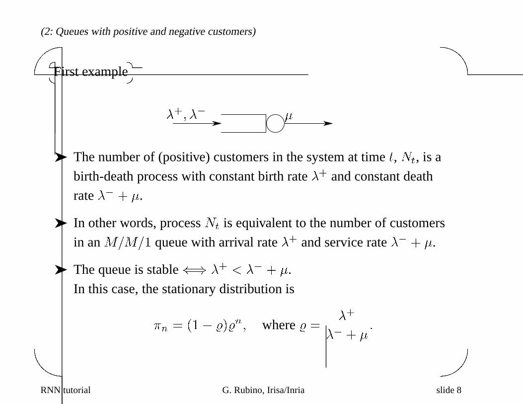
� ��First example

��

➤ The number of (positive) customers in the system at timet, Nt, is a

birth-death process with constant birth rate�� and constant death

rate�� .

➤ In other words, processNt is equivalent to the number of customers

in anM�M�� queue with arrival rate�� and service rate�� .

➤ The queue is stable�� .

In this case, the stationary distribution is

�n � �� n� where� �

��

��



��

� ��Some details on the analysis

➤ Let pn�t� � Pr�Nt � n�.

➤ Start frompn�t� ��

�Xk��

Pr�Nt�� n j Nt � k�pk�t��

➤ Whenjn� kj � �, then

Pr�Nt�� n j Nt � k� � o��

➤ Now,

Pr�Nt�� n j Nt � n� �� o��

Pr�Nt�� n j Nt � n� �� o��

Pr�Nt�� n j Nt � n� � �� o��



��

� ��Some details on the analysis (cont.)

This leads to

pn�t� ��

��pn��t�� pn��t�� pn�t� � o��

➤ Passingpn�t� to the left, dividing by� and letting� �� we get

p�n�t� � ��pn��t� � �� pn��t�� pn�t��

➤ Denoting�n � limt�� pn�t� and assuming stability, we get

�� n � ��n�� n��

➤ Looking for a solution of the form�n � abn we get

�n � �� n� where� �

��

��



��

� ��Another basic example

Consider the model represented here:

��

➤ External arrivals are positive.

➤ Once served, customers come back as negative ones.

➤ The graph of the process “# of customers in the system at timet” is

given in the following scheme:

0 3 4

��

� � �

�� 1 2



��

� ��Another basic example (cont.)

➤ If we look for a solution to the equilibrium equations of the form

�n � abn, that is,�n � �� b�bn, b must verifyb� � b� � � and � � b � ��

where � ��.

➤ We obtain

b �p

� � � �

�

�under the (stability) condition�� .



��

� ��Another basic example (cont.)

➤ Call T� (respectivelyT�) the mean throughput ofarriving positive

(resp. negative) customers; we have

� T� � ��,

� T� � �� b�.

➤ See that

� � b �

T�

�� T��

��

�� b��

since this means that

b �

� � b�� b� � b � �


3: Networks with positive and negative customers��

��

� �A 2-nodes network

Consider the following network:�

p��

‘-’

‘+’ ��

�� p

We can write the equilibrium equations and solve them.

Assume equilibrium and write�ij for the stationary probability of having

i units at 1 andj units at 2. We obtain

➤ ��

➤ �i�� i�� i��p� �i�� p� � �i��

➤ ��j�� j�� i��j��p� �i��j�� p�

➤ �ij��

�i��j�� i��j��p� �i��j�� p� � �i�j��RNN tutorial G. Rubino, Irisa/Inria slide 14

(3: Networks with positive and negative customers)��

��

� �A 2-nodes network

➤ Since the first node clearly behaves as aM�M�� queue, we can

guess a solution with�i�j proportional toaibj , wherea � ��.

➤ We obtain an equation forb and the solution

b �

�p

�� p��

➤ Another way: Burke’s theorem says that, in steady-state, the output

of node 1 is Poisson (with parameter�, of course). This leads to a

second queue as in our first example, with arrival rates�p for positive

customers and�� p� for negative customers, and the already given

b value.

➤ Again, see that for each nodei, �i � T�i ��i � T�i � whereT�i and

T�i are defined as before,i � �� .



��

� ��The general network model

➤ # of nodes:N➤ service rate at nodei: �i

➤ routing probabilities: when leaving nodei, a customer

goes to nodej as a positive one with probabilityr�ij ,

as a negative one with probabilityr�ij ,

and it leaves the network with probabilitydi.

We then have

di �

NXj��

�r�ij � r�ij�

� ��➤ From outside, the arrival rate of positive customers at nodei is ��i ,

and of negative customers is��i .



��

� ��The traffic equations

➤ Let T�i be the mean throughput of positive customers thatenter

nodei. Assuming equilibrium, we have

T�i � ��i �X

j

�j�jr�

ji�

where�j is the probability that nodej is busy.

➤ If T�i is the mean throughput of negative customers thatenter nodei

in equilibrium,

T�i � ��i �X

j

�j�jr�

ji�



��

➤ Add the following equations

�i �

T�i

�i � T�i�

as in the simple previous examples. We obtain a (non linear) system

with N equations andN unknowns (theT�i ’s, theT�i ’s and the

�i’s).

➤ It can be shown that this linear system has an unique solution (fixed

point theory).



��

➤ If in that solution, we have that for all nodei, �i � �, then thenetwork is stable and it has aproduct-form equilibrium distribution:

for all n� � �� nN � �,

�n�� nN �

NYi��

�� i��ni

i �

➤ Corollary: we have

� asymptotic independence between nodes;

� geometric marginals:Pr�n at i, in equilibrium� � �� i��n

i �

� the�i’s are indeed the utilization ratios:

Pr�i busy, in equilibrium� � �i�

➤ This model has several extensions (more complex behaviour ofnegative customers, multiclass populations). Some of them arerelevant in the RNN context, but we will focus here on the basicmodel.



��

� ��Example: a general 2-nodes network without loops

➤ We have to solve the non-linear system in��

��

�� r�

��

�� r�

��

��

�� r�

��

�� r�

��

➤ Denotingw�ij � �ir�

ij

andw�ij � �ir�

ij ,

the system becomes

��

�� w��

�� w��

��

�� w��

�� w��



��

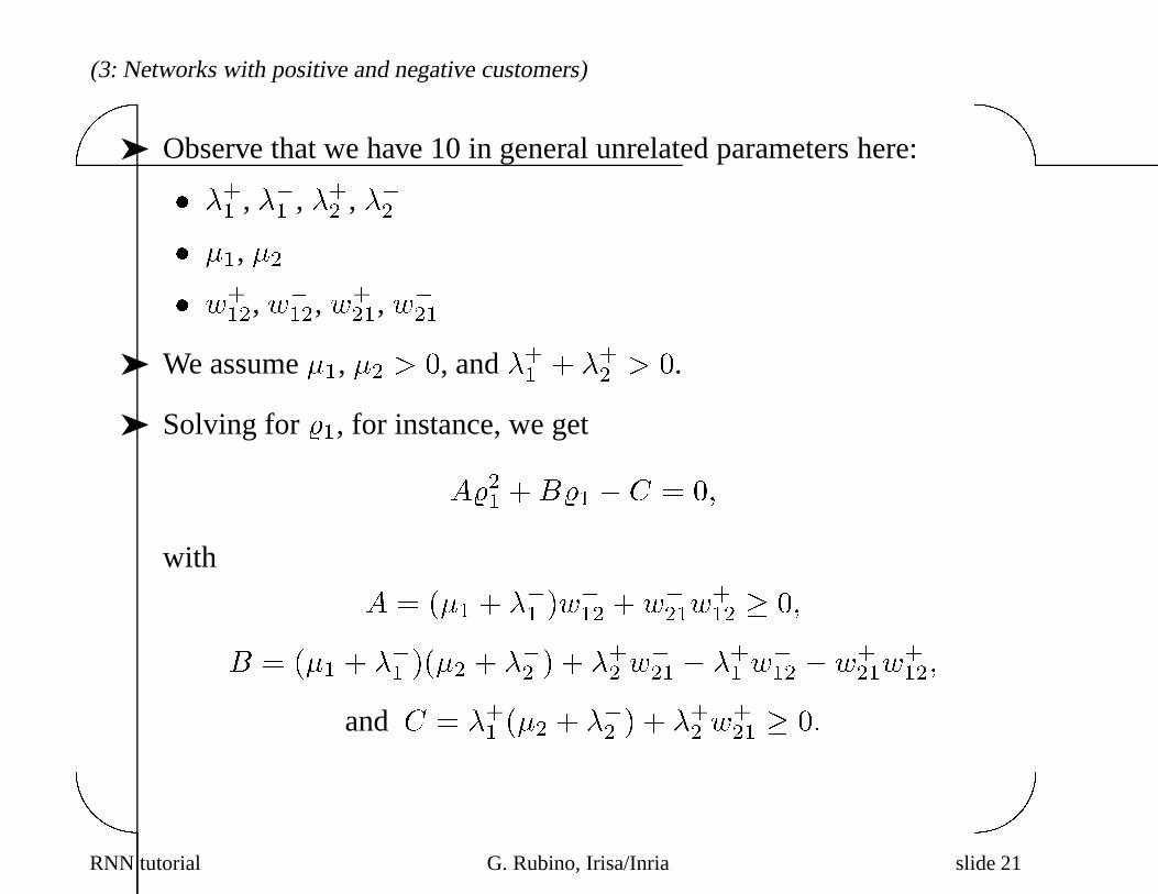
➤ Observe that we have 10 in general unrelated parameters here:� �� , �� , �� , ��

� ��, ��

� w��, w�

��, w�

��, w�

��

➤ We assume��, �� , and�� .

➤ Solving for��, for instance, we getA�� B�� C � ��

with

A � �� w�

�� w��w�

��

B � �� w�

�� w�

�� w��w�

��

and C � �� w�

��



��

➤ It can be checked that if we exclude the case of a system being

always unstable,� � B� � AC �.

➤ Thus, the equation has two real roots of opposite signs. This means

that the only relevant one is

�� B �p

�

�A

�

➤ After some algebra, we have�� C � A�B�

This is a complex but explicit expression of the stability condition for

such a model.


4: Random Neural Networks��

��

� �G-networks as Neural Networks

Just change

➤ node, or queue, by neuron

➤ # of customers at node i by potential of neuron i

➤ positive customer arrival by exciting signal

➤ negative customer arrival by inhibiting signal

➤ � � �

that is, the mathematical model is exactly the same. We look at the

dynamical system just differently.

➤ If at t, the backlog ati (the potential ati) is �, we say that neuroni

is excited at t.


(4: Random Neural Networks)��

��

� ��Weights

➤ For any pair of nodesi, j, such asdi � �, define

w�ij � �ir�

ij � w�ij � �ir�

ij�

➤ If di � � for somei, we definew�ij � w�ij � � for all j

➤ Observe thatw�ij (resp.w�ij) is the mean throughput of positive (resp.

negative) signals fromi to j

➤ The mean throughput of positive and negative customers entering

nodei can be respectively written as

T�i � ��i �X

j

�jw�

ji� T�i � ��i �X

j

�jw�

ji�RNN tutorial G. Rubino, Irisa/Inria slide 24


��

� ��3-layer models

➤ This a basic class of models (a particular type offeedforward

topology).

➤ Consider a G-network with three classes of nodes:

� I = the “input” nodes: they receive customers from outside; they

are connected to the “internal” of “hidden” nodes only;

� O: the “output” nodes: they send out customers, they receive no

flows from outside, and they receive customers from the hidden

ones

� H: the hidden nodes, with no connexion with the environment,

receiving fromI and sending toO

➤ the service rate at nodek is �k



��

� ��3-layer models (cont.)

➤ After its service ati � I, a customer goes toh � H as a positive one

with probabilityr�ih, and as a negative one with probabilityr�ih.

➤ After its service ath � H, a customer goes too � O as a positive one

with probabilityr�ho, and as a negative one with probabilityr�ho.

➤ After its service ato � O, the customer leaves the network.



��


➤ For all input nodei,

T�i � ��i � T�i � ��i � �i �

��i

�i � ��i�

➤ For all hidden nodeh,

T�h �X

i�I�i�ir�

ih� T�h �X

i�I�i�ir�

ih�

➤ For all output nodeo,

T�o �X

h�H

�h�hr�

ho� T�o �X

h�H

�h�hr�

ho�

➤ In this class of model, the non linear system can be explicitly solved.



��


➤ Recall that for any pair of nodesi, j such thatdi � � (that is,i � O),

w�ij � �ir�

ij � w�ij � �ir�

ij�

➤ Then for all hidden nodeh,

T�h �X

i�I�iw�

ih� T�h �X

i�I�iw�

ih�

➤ and for all output nodeo,

T�o �X

h�H

�hw�

ho� T�o �X

h�H

�hw�

ho�



��


Stability conditions:

➤ for all i � I, ��i � ��i � �i,

➤ for all h � H, T�h � T�h � �h,

➤ for all o � O, T�o � T�o � �o.

If ��i � ��

i ��, then sufficient conditions for stability,for all �w, are

➤ for all i � I, �i � �,

➤ and for allh � H ando � O, �h � �o � I.



��

� ��RNN in learning

➤ Assume an unknown functionf�� from IRI into IRO is known only

throughK pairs of input-output values.

➤ RNN can be used as an interpolator-extrapolator tool, performing a

statistical learning of the set of input-output values.

➤ To simplify the presentation, assume that we can normalize the input

and output variables into��, that is, that

f ��I � ��O�➤ Data: the setD of K pairs��ak��bk�, k � ��K, wheref��ak� � �bk.



��

� ��RNN in learning (cont.)

➤ Now, consider a 3-layer RNN. Assume that there are no negative

customers coming from outside (��i � � for all i).

➤ The RNN hasI input nodes andO output nodes.

➤ Look at the RNN as an input-output system:

� the input is the vector�� I �;

� the output is the vector�� O�;

� to simplify, we assume the service rates fixed, and we look at the

set of weights as parameters; we denote�w � fw�ijg;

� the�i’s can be set to assure stability, or to leave instability as a

possible case;

� as an input-output system, the RNN maps�� into �� w� � ��.



��

� ��RNN in learning (cont.)

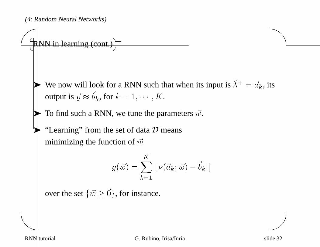
➤ We now will look for a RNN such that when its input is�� ak, its

output is�� bk, for k � �� K.

➤ To find such a RNN, we tune the parameters�w.

➤ “Learning” from the set of dataD means

minimizing the function of�w

g��w� �

KXk��jj��ak� �w��bkjj

over the setf�w � ��g, for instance.



��

� ��Learning (cont.)

Basic approach for the optimization problem (gradient descent): write

g��w� ��

�KX

k��X

o�O

h�o��ak� �w�� bk�oi�

Then, iterate over the following:

w�ij�m� ��

w�ij�m�� g

�w�ij��w�m��

��

w�ij�m� ��

w�ij�m�� g

�w�ij��w�m��

��

Factor is thelearning rate of the model.



��


➤ It must be observed that, since�� is infinitely differentiable, so is

g��.

➤ Moreover, the product form of�� allows an efficient computation of

derivatives.

➤ This means that the learning procedure can take advantage of

standard numerical procedures (and is open to further progress the

same way).



��


➤ More precisely: partition theK data pairs randomly (uniformly) into

two subsets:f��ak��bk�� k � ��K �g andf��ak��bk�� k � K� � ��Kg.➤ Learning � solving the optimization problem

find �� argmin�w��K�X

k��jj��ak� �w��bkjj�

➤ If

� the�ak ’s, for k � ��K� “reasonably” cover the possible input

values off�� (the domain�� I ),

� and iff�� has some properties (bounded derivatives,� � � )

we expect the RNN�� accurately approximatingf�� over the

whole �� I .



��

➤ Validation � evaluating

Err �

KXk�K��jj��ak� �w��bkjj�

and “accepting”�� if Err � �.

➤ If Err � �, probably more data is needed.

➤ Other possibilities are

� a too small number of hidden neurons;

� a too large number of hidden neurons;



��

� ��On RNN in optimization

➤ For optimization problems, the approaches are strongly dependent on

the problem.

➤ In particular, the topologies of the RNN are strongly dependant on

the problem.

➤ However, an usual pattern is to look for unstable nodes in the models.

➤ Section 6 of this tutorial describes in detail a specific application of

RNN in the optimization area.


5: PSQA: Pseudo-Subjective Quality Assessment��

��

� ��QQA: Quantitative Quality Assessment

➤ The problem:

1. quantify the quality of a video or audio or multimedia stream

transmitted over the Internet,

2. as perceived by the end user (observer),

3. automatically

4. and, if necessary, in real time.

➤ The first two points can be efficiently done with real human

observers.

➤ Name of the field:subjective testing.

➤ Standardized activity.

➤ Subjective testing is not real time, nor automatic.


(5: PSQA: Pseudo-Subjective Quality Assessment)��

��

� ��QQA (cont.)

➤ Objective testing: basically, tools to compare the original and theencoded stream (both at the source).

➤ It takes the formd�� where� is the original sequence,�� theencoded one, andd�� is some distance function.

➤ The original sequence is thus needed.

➤ One “pseudo-exception”: the E-model (for VoIP).

➤ Some tentative objective measures taking the form of a simpleformula of one or two parameters have been published, of the type

Q �

�BR

�LR � �

or Q �

�BR�

�LR� � �

where LR = loss rate, BR = bit rate, Q = quality.

➤ Common (negative) point: objective measures (anyway) correlateoften badly with subjective testing.



��

� ��PSQA

➤ Using RNNs, we propose a solution to the problem, that is

� an accurate metric measuring perceived user quality,

� evaluated automatically and very efficiently (so, being able to

work in real time),

� called PSQA: Pseudo-Subjective Quality Assessment.



��

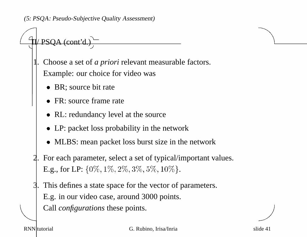
� ��II/ PSQA (cont’d.)

1. Choose a set ofa priori relevant measurable factors.

Example: our choice for video was

� BR; source bit rate

� FR: source frame rate

� RL: redundancy level at the source

� LP: packet loss probability in the network

� MLBS: mean packet loss burst size in the network

2. For each parameter, select a set of typical/important values.

E.g., for LP:f�� g.3. This defines a state space for the vector of parameters.

E.g. in our video case, around 3000 points.

Call configurations these points.



��

4. Select a sample set of sizeN (e.g.,N � ��) points (this must bedone with a merge of random sampling and covering criteria).

5. Select randomlyN � points between this sample. E.g.N � � ��.Renumber them��N �; theN �N � remaining configs. are

N � � ��N .

6. Build a testbed or a simulator allowing to control the chosenparameters.

7. Start from a sequence� (say, 10 sec. length) and send itN� times tothe receiver according to theN � different configs.The result is a setf�� N �g of distorted copies of�.

8. PutK humans (K ��) to evaluate theseN � sequences according toa standardized subjective test.Let �ik be the value given to sequence�i by observerk.

9. Perform a statistical filtering of thef�ikg having as a goal to detectthe bad observers, and eliminate the associated evaluations.



��

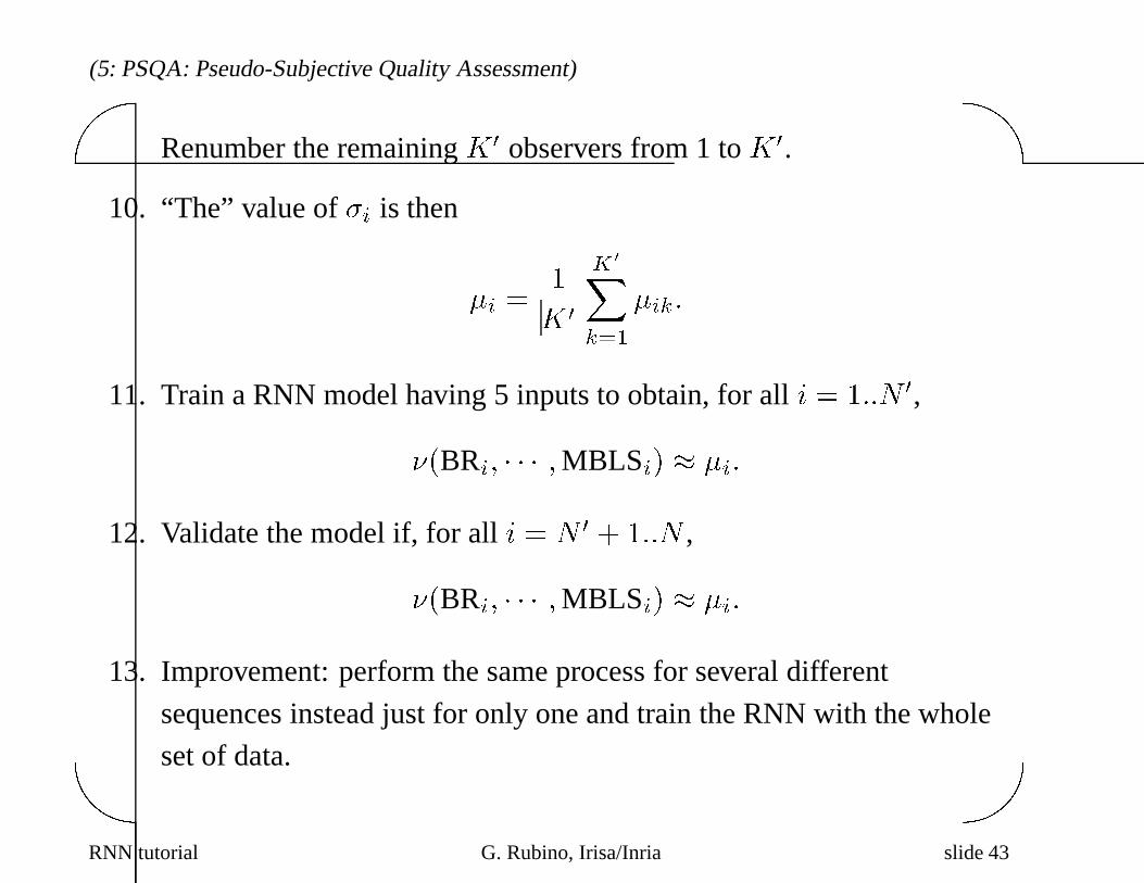
Renumber the remainingK� observers from 1 toK�.

10. “The” value of�i is then

�i �

�K�

K�Xk��

�ik�

11. Train a RNN model having 5 inputs to obtain, for alli � ��N �,��BRi� � � � �MBLSi� �i�

12. Validate the model if, for alli � N � � ��N ,

��BRi� � � � �MBLSi� �i�

13. Improvement: perform the same process for several different

sequences instead just for only one and train the RNN with the whole

set of data.


6: WAN design��

��

� ��The problem

➤ A WAN is in general divided into abackbone (high speed, high

connectivity) and anaccess network (forest-like topology).

➤ Assume the backbone is designed, and we must now select the

optimal architecture for the access network.

➤ The access network has two types of nodes:terminals and

concentrators; backbone nodes areswitches.

➤ Terminals can not be connected between them.


(6: WAN design)��

��

� ��The problem (cont.)

An example of the whole network topology.

sc

sc

sc

sc

sc

sc

sc

sc

sc

BackboneNetwork

Terminal Site

sc Concentrator Site

Switch SiteA local access network



��


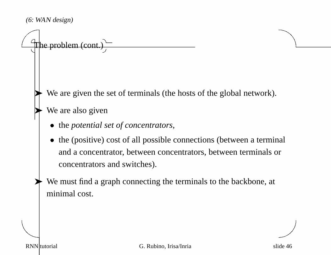
➤ We are given the set of terminals (the hosts of the global network).

➤ We are also given

� thepotential set of concentrators,

� the (positive) cost of all possible connections (between a terminal

and a concentrator, between concentrators, between terminals or

concentrators and switches).

➤ We must find a graph connecting the terminals to the backbone, at

minimal cost.



��


➤ In real size problems, the combinatory complexity is too high, and anexact solution is not possible.

➤ This means that many heuristics have been applied to solve theproblem.

➤ Usual approach:

� build an initial topology;

� make “small” changes to this initial graph, trying to improve it(reducing the cost); many solutions here;

� repeat the two previous steps, and keep the best of all foundtopologies.

➤ Remark: This description covers the essentials; the same difficultiesappear (and the same approaches apply) in problems with moreconstraints.



��

� ��A GRASP solution using RNN

➤ GRASP stands for Greedy Randomized Adaptive Search Procedure),

a powerful family of methods shown to be successful in many

optimization problems.

➤ The procedure starts by building a possible topology (this is the

construction phase).

➤ Then, this topology is improved using an appropriate RNN (this is

theimprovement phase).

➤ The two previous steps are repeated a numberN of times.

➤ At the end, the best of theN topologies having been built is returned.

➤ Before starting, we collapse the backbone into a single nodez.

➤ Recall that data is composed of the graph of all possible connections,

together with the associated costs.



��

� ��A GRASP solution using RNN: construction phase

➤ We will connect the terminals one after the other to nodez.

➤ At the beginning, no terminal is marked (marked as “already

included in the current solution”).

➤ A path in the initial graph (with all possible connections) isvalid if it

starts at a terminal, it ends atz, and it includes any number of

concentrators (possibly none) but not another terminal.



��

� ��A GRASP solution using RNN: construction phase (cont’d)

The construction procedure is as follows:

1. Initialize the setC throughC � fzg.2. Pick a non marked terminalt at random; mark it.

3. Compute theK shortest (minimum cost) valid paths fromt to C.

4. Pick one of these paths randomly, and add it to the current solution

(its nodes and links are added toC).

5. Repeat the previous steps until all terminals are marked.



��

� ��A GRASP solution using RNN: improvement phase

➤ Data: a graphG connecting the terminals to nodez with only valid

paths.

➤ If �i� j� � G, the cost of the connection isci�j .

➤ We denote byc the average cost of the links.

➤ The classical approaches call this part of the algorithm thelocal

search phase because the improvement is made in some

neighbourhood of the graph (ideas fromgenetic algorithms,

simulated annealing,...).



��

� ��A GRASP solution using RNN: improvement phase (cont.)

Here, we build and solve a RNN defined in the following way (the

mapping comes from another paper by E. Gelenbe, on a similar problem):

➤ For each node in the graph there is a neuron in the RNN.

➤ If �i� j� � G thenw�i�j �

cci�j

.

➤ If �i� j� � G then, in the RNN we setw�i�j � �.

➤ The remaining weights are set to�.

➤ For each nodei, its service rate is defined as

�i �X

j

�w�i�j � w�i�j��

➤ There is no external arriving flow.



��

➤ The terminals and the concentrators belonging to the solution (plus

nodez) are artificially excited: the corresponding neurons receive an

infinite potential and, in fact, they act assources in the model.

➤ The loads in the different nodes are evaluated. Letc be the

concentrator having the highest load.

➤ If c is not in the initial solution, then its inclusion in a new solution

is explored through a local (in the graph) procedure addingc and

removing other concentrators. If a better solution is found, the

procedure starts again from the new topology.

➤ If c is already in the solution, its load is set to 1 and the procedure is

run again.

➤ The improvement phase stops when all concentrators have been

examined for inclusion in the solution.



��

� ��A GRASP solution using RNN: improvement phase (cont.)

➤ Observe that if a neuron is excited and its connections with its

neighbours have low costs (and so, high excitatory rates to them),

then it will have a high influence on those neighbours.

➤ We have explored other possibilities for this improvement phase, and

RNN outperforms them:

� We can pick a new concentrator at random (i.e. uniformly) among

the not yet considered ones.

� We can also compute, for all concentratorc not in the current

solution, the sumS�c� of the cost of all the links arriving to it,

and selectc� � argmincS�c�.

➤ The reason of the good performance of RNN is that instead of using

local information, the RNN allows to integrate the dynamics of the

whole network at each step it is used.



��

� ��Some computational examples

➤ We used a large test set, obtained by modifying the Steiner Problem

instances in the well known SteinLib repository.

➤ Parameter settings (from GRASP literature):

� candidate list size:��,

� maximum number of iterations:��.

➤ Equipment: Pentium IV with 1.7 GHz, 1 Gbytes of RAM, Windows

XP.



��

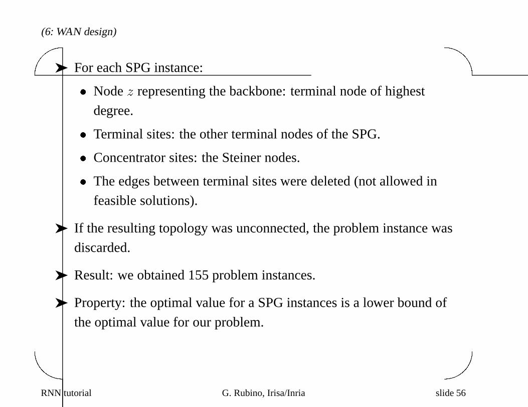
➤ For each SPG instance:� Nodez representing the backbone: terminal node of highest

degree.

� Terminal sites: the other terminal nodes of the SPG.

� Concentrator sites: the Steiner nodes.

� The edges between terminal sites were deleted (not allowed in

feasible solutions).

➤ If the resulting topology was unconnected, the problem instance was

discarded.

➤ Result: we obtained 155 problem instances.

➤ Property: the optimal value for a SPG instances is a lower bound of

the optimal value for our problem.



��

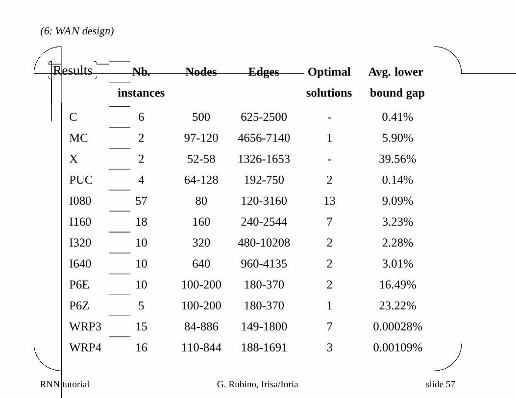
� �Results Nb. Nodes Edges Optimal Avg. lower

instances solutions bound gap

C 6 500 625-2500 - 0.41%

MC 2 97-120 4656-7140 1 5.90%

X 2 52-58 1326-1653 - 39.56%

PUC 4 64-128 192-750 2 0.14%

I080 57 80 120-3160 13 9.09%

I160 18 160 240-2544 7 3.23%

I320 10 320 480-10208 2 2.28%

I640 10 640 960-4135 2 3.01%

P6E 10 100-200 180-370 2 16.49%

P6Z 5 100-200 180-370 1 23.22%

WRP3 15 84-886 149-1800 7 0.00028%

WRP4 16 110-844 188-1691 3 0.00109%



��

� �More results Nb. Nodes Edges Avg. LS Avg. exec.

inst. improv. times (s/itr

C 6 500 625-2500 19.95% 12.13

MC 2 97-120 4656-7140 24.89% 2.07

X 2 52-58 1326-1653 11.00% 0.73

PUC 4 64-128 192-750 21.04% 1.27

I080 57 80 120-3160 17.01% 0.85

I160 18 160 240-2544 21.46% 3.18

I320 10 320 480-10208 24.93% 9.2

I640 10 640 960-4135 24.33% 27.15

P6E 10 100-200 180-370 23.75% 1.83

P6Z 5 100-200 180-370 22.01% 1.10

WRP3 15 84-886 149-1800 20.3% 17.00

WRP4 16 110-844 188-1691 32.36% 22.56



��

� �Some remarks

➤ The results on the benchmark set show good quality solutions.

➤ In 40 cases (out of 155) the lower bound was reached (implying

optimality).

➤ In most cases the gap with respect to the known lower bound was

quite small (less than 5% on the average, in 7 out of 12 problem

classes).

➤ The underlying RNN improved significantly the solutions delivered

by the construction phase: over 20% of improvement, on the average,

for most problem classes (and always over 10%).


7: Bibliography��

��

� ��Basic papers

The RNN model was introduced by Erol Gelenbe mainly in the following

papers:

➤ Random neural networks with negative and positive signals andproduct form solution. E. Gelenbe. InNeural Computation,

1(4):502–511, 1989.

➤ Stability of the random neural network model. E. Gelenbe. In

Neural Computation, 2(2):239–247, 1990.

➤ Learning in the recurrent random neural network. E. Gelenbe. In

Neural Computation, 5(1): 154–511, 1993.


(7: Bibliography)��

��

� ��Applications of RNN and related topics

See also Vol. 126, Issue 2, 2000, of European Journal of Operations

Research, on G-networks, and the numerous references in the papers of

this special issue.

To give a few specific examples,

➤ In learning, for instance

� Random Neural Network Filter for Land Mine Detection.

H. Abdelbaki, E. Gelenbe, T. Koc¸ak and S. El-Khamy. In

NRSC’99, El Cairo, Egypt, February 1999.

� Pictorial Information Retrieval Using the Random NeuralNetwork. A. Stafylopatis and A. Likas. InIEEE TRans. on

Software Engineering, 18(7): 590–600, 1992.



��

➤ In optimization,� Using the General Energy Function of the Random Neural

Networks to solve the Graph Partitioning Problem. J. Aguilar.

In Proc. of the Int. Conf. on Neural Networks, IEEE Neural

Networks Council, pp. 2130–2135, Washington, D.C., USA, June

1996.

� A Qualitative Comparison of Neural Network Models Appliedto the Vertex Covering Problem. A. Ghanwani. InELEKTRIK,

2(1), April 1994.

➤ Other topics where RNNs have been successfully used: Travelling

Salesman Problem, Error Correction Codes, Image Compression,

application in Magnetic Resonance Imaging, Texture Generation,

Packet Network Routing,...



��

� �Our work

Details on the PSQA approach and the analysis of the impact of different

factors on quality:

➤ for video, seeA Study of Real-Time Packet Video Quality UsingRandom Neural Networks, S. Mohamed and G. Rubino,IEEE

Transactions on Circuits and Systems for Video Technology, 12(12),

2002;

in this paper, some comparisons between standard Neural Networks

and RNNs are provided (showing that for this application at least,

RNNs are superior);



��

➤ for audio, seePerformance Evaluation of Real-time SpeechThrough a Packet Network: a Random Neural Network BasedApproach, S. Mohamed, G. Rubino, M. Varela,Performance

Evaluation, 57 (2), 2004;

some comments are given here on other possible tools (as Bayesian

networks; again, RNNs appear to be superior).



��

� ��Our work (cont’d)

A more recent work resuming the PSQA technique is

➤ Using Random Neural Networks to quantify the quality of audioand video transmissions over the Internet: the PSQA approach,

G. Rubino,Design and Operations of Communication Networks: A

Review of Wired and Wireless Modelling and Management

Challenges, ed. by J. Barria, ICP, UK, 2005;



��


➤ for performance evaluation aspects, seeA new approach for theprediction of end-to-end performance of multimedia streams,G. Rubino and M. Varela, in QEST’04, IEEE CS Press, Sept. 2004,Twente, Netherlands;

➤ for an application of our approach to FEC analysis in VoIP, seeEvaluating the utility of media-dependent FEC in VoIP flows,G. Rubino and M. Varela, in Lecture Notes in Computer Science3266, Springer Verlag, 2004.

➤ for some complementary comparisons with other approachesattempting to handle quality (audio), seeA method for quantitativeevaluation of audio quality over packet networks and itscomparison with existing techniquesS. Mohamed, G. Rubino and M. Varela, in MESAQUIN’04, Prague,June 2004).



��


➤ See alsoWireless VoIP at Home: Are We There Yet?. G. Rubino,

M. Varela and J.-M. Bonnin, In MESAQUIN’05, Prague, June 2005.

Concerning the case study in WAN design, see

➤ A GRASP algorithm with RNN based local search for designing aWAN access network. H. Cancela, F. Robledo and G. Rubino. In

LACGA’04, Santiago, Chile, August 2004.

(For an extensive bibliography on GRASP, go to

http://www.research.att.com/˜mgcr/

grasp/gannbib/gannbib.html

)


A tutorial on Random Neural Networks - IRISA · A tutorial on Random Neural Networks G. Rubino...

Documents

Transcript of A tutorial on Random Neural Networks - IRISA · A tutorial on Random Neural Networks G. Rubino...