A Tutorial on Deep Learning for Music InformationRetrieval

Keunwoo Choikeunwoo.choi@qmul.ac.uk

György Fazekasg.fazekas@qmul.ac.uk

Kyunghyun Chokyunghyun.cho@nyu.edu

Mark Sandlermark.sandler@qmul.ac.uk

ABSTRACTFollowing their success in Computer Vision and other ar-eas, deep learning techniques have recently become widelyadopted in Music Information Retrieval (MIR) research. How-ever, the majority of works aim to adopt and assess methodsthat have been shown to be effective in other domains, whilethere is still a great need for more original research focus-ing on music primarily and utilising musical knowledge andinsight. The goal of this paper is to boost the interest ofbeginners by providing a comprehensive tutorial and reduc-ing the barriers to entry into deep learning for MIR. Welay out the basic principles and review prominent works inthis hard to navigate field. We then outline the networkstructures that have been successful in MIR problems andfacilitate the selection of building blocks for the problems athand. Finally, guidelines for new tasks and some advancedtopics in deep learning are discussed to stimulate new re-search in this fascinating field.

1. MOTIVATIONIn recent years, deep learning methods have become more

popular in the field of music information retrieval (MIR)research. For example, while there were only 2 deep learn-ing articles in 2010 in ISMIR conferences 1 ([30], [38]) and6 articles in 2015 ([123], [91], [97], [65], [36], [10]), it in-creases to 16 articles in 2016. This trend is even strongerin other machine learning fields, e.g., computer vision andnatural language processing, those with larger communitiesand more competition. Overall, deep learning methods areprobably going to serve an essential role in MIR.

There are many materials that focus on explaining deeplearning including a recently released book [34]. Some of thematerial specialises on certain domains, e.g., natural lan-guage processing [33]. In MIR, there was a tutorial sessionin 2012 ISMIR conference, which is valuable but outdatedas of 2017.2

Much deep learning research is based on shared modulesand methodologies such as dense layers, convolutional lay-ers, recurrent layers, activation functions, loss functions, andbackpropagation-based training. This makes the knowledgeon deep learning generalisable for problems in different do-mains, e.g., convolutional neural networks were originally

1http://www.ismir.net2http://steinhardt.nyu.edu/marl/research/deep_learning_in_music_informatics

.

used for computer vision, but are now used in natural lan-guage processing and MIR.

For these aforementioned reasons, this paper aims to pro-vide comprehensive basic knowledge to understand how andwhy deep learning techniques are designed and used in thecontext of MIR. We assume readers have a background inMIR. However, we will provide some basics of MIR in thecontext of deep learning. Since deep learning is a subsetof machine learning, we also assume readers have under-standing of the basic machine learning concepts, e.g., datasplitting, training a classifier, and overfitting.

Section 2 describes some introductory concepts of deeplearning. Section 3 defines and categorises the MIR prob-lems from the perspective of deep learning practitioners.In Section 4, three core modules of deep neural networks(DNNs) are described both in general and in the contextof solving MIR problems. Section 5 suggests several mod-els that incorporate the modules introduced in Section 4.Section 6 concludes the paper.

2. DEEP LEARNINGThere were a number of important early works on neural

networks that are related to the current deep learning tech-nologies. The error backpropagation [84], which is a way toapply the gradient descent algorithm for deep neural net-works, was introduced in the 80s. A convolutional neuralnetwork (convnet) was used for handwritten digit recogni-tion in [56]. Later, long short-term memory (LSTM) recur-rent unit was introduced [42] for sequence modelling. Theystill remain the foundation of modern DNN algorithms.

Recently, there have been several advancements that havecontributed to the success of the modern deep learning. Themost important innovation happened in the optimisationtechnique. The training speed of DNNs was significantlyimproved by using rectified linear units (ReLUs) instead ofsigmoid functions [32] (Section 2.1, Figure 3). This led toinnovations in image recognition [53] and speech recogni-tion [22] [122]. Another important change is the advance inhardware. Parallel computing on graphics processing units(GPUs) enabled Krizhevsky et al. to pioneer a large-scalevisual image classification in [53].

Let us explain and define several basic concepts of neuralnetworks before we discuss the aspects of deep learning.

A node is analogous to a biological neuron and representsa scalar value as in Figure 1 (a). A layer consists of a set ofnodes as in Figure 1 (b) and represents a vector. Note thatthe nodes within a layer are not inter-connected. Usually, anactivation function f() is applied to each node as in Figure

arX

iv:1

709.

0439

6v2

[cs

.CV

] 3

May

201

8

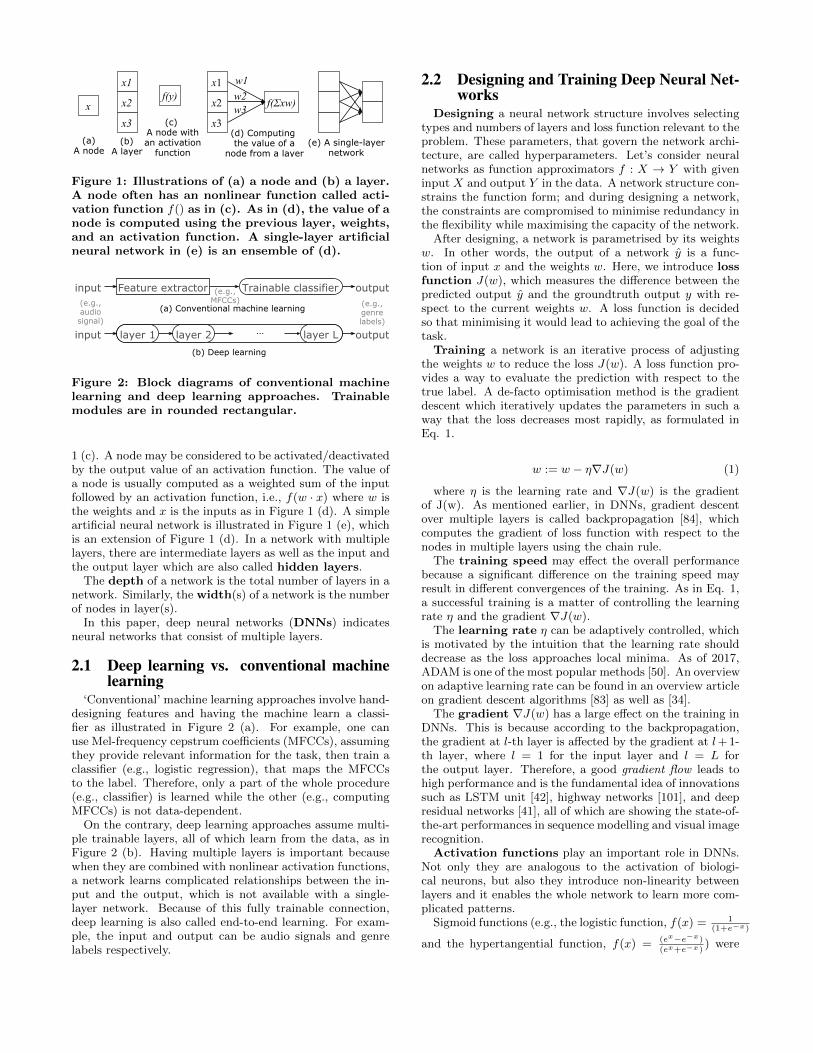
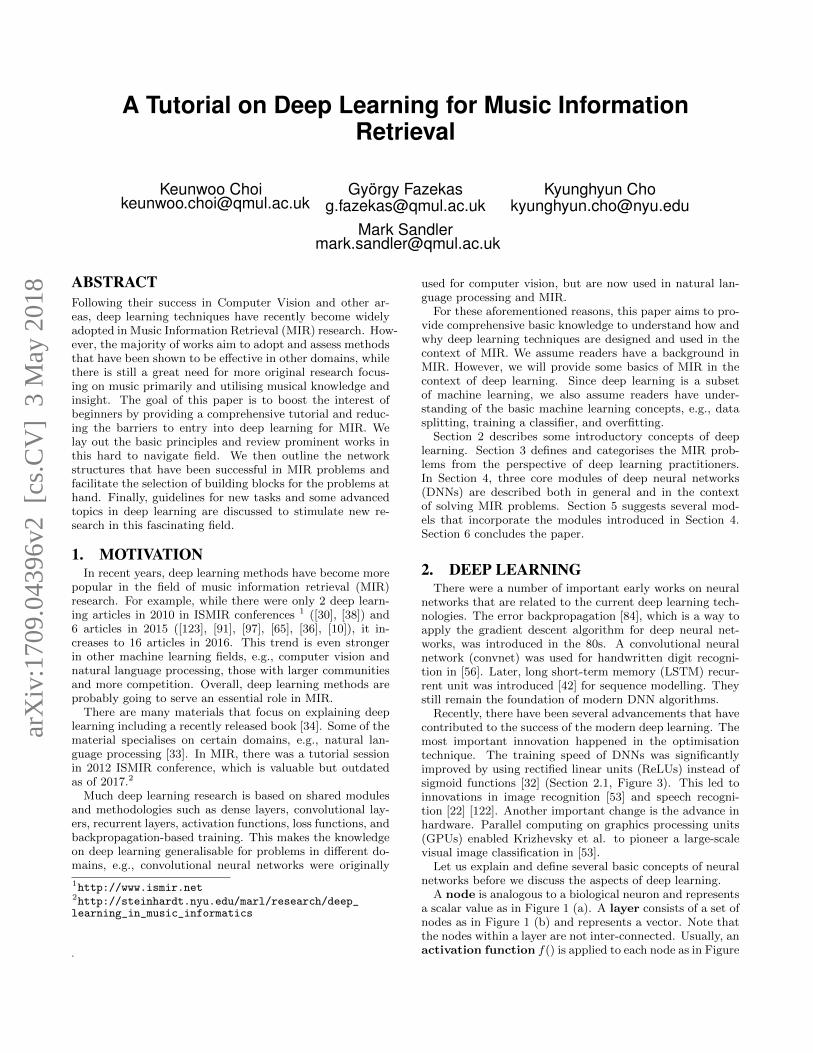
Figure 1: Illustrations of (a) a node and (b) a layer.A node often has an nonlinear function called acti-vation function f() as in (c). As in (d), the value of anode is computed using the previous layer, weights,and an activation function. A single-layer artificialneural network in (e) is an ensemble of (d).

Figure 2: Block diagrams of conventional machinelearning and deep learning approaches. Trainablemodules are in rounded rectangular.

1 (c). A node may be considered to be activated/deactivatedby the output value of an activation function. The value ofa node is usually computed as a weighted sum of the inputfollowed by an activation function, i.e., f(w · x) where w isthe weights and x is the inputs as in Figure 1 (d). A simpleartificial neural network is illustrated in Figure 1 (e), whichis an extension of Figure 1 (d). In a network with multiplelayers, there are intermediate layers as well as the input andthe output layer which are also called hidden layers.

The depth of a network is the total number of layers in anetwork. Similarly, the width(s) of a network is the numberof nodes in layer(s).

In this paper, deep neural networks (DNNs) indicatesneural networks that consist of multiple layers.

2.1 Deep learning vs. conventional machinelearning

‘Conventional’ machine learning approaches involve hand-designing features and having the machine learn a classi-fier as illustrated in Figure 2 (a). For example, one canuse Mel-frequency cepstrum coefficients (MFCCs), assumingthey provide relevant information for the task, then train aclassifier (e.g., logistic regression), that maps the MFCCsto the label. Therefore, only a part of the whole procedure(e.g., classifier) is learned while the other (e.g., computingMFCCs) is not data-dependent.

On the contrary, deep learning approaches assume multi-ple trainable layers, all of which learn from the data, as inFigure 2 (b). Having multiple layers is important becausewhen they are combined with nonlinear activation functions,a network learns complicated relationships between the in-put and the output, which is not available with a single-layer network. Because of this fully trainable connection,deep learning is also called end-to-end learning. For exam-ple, the input and output can be audio signals and genrelabels respectively.

2.2 Designing and Training Deep Neural Net-works

Designing a neural network structure involves selectingtypes and numbers of layers and loss function relevant to theproblem. These parameters, that govern the network archi-tecture, are called hyperparameters. Let’s consider neuralnetworks as function approximators f : X → Y with giveninput X and output Y in the data. A network structure con-strains the function form; and during designing a network,the constraints are compromised to minimise redundancy inthe flexibility while maximising the capacity of the network.

After designing, a network is parametrised by its weightsw. In other words, the output of a network y is a func-tion of input x and the weights w. Here, we introduce lossfunction J(w), which measures the difference between thepredicted output y and the groundtruth output y with re-spect to the current weights w. A loss function is decidedso that minimising it would lead to achieving the goal of thetask.

Training a network is an iterative process of adjustingthe weights w to reduce the loss J(w). A loss function pro-vides a way to evaluate the prediction with respect to thetrue label. A de-facto optimisation method is the gradientdescent which iteratively updates the parameters in such away that the loss decreases most rapidly, as formulated inEq. 1.

w := w − η∇J(w) (1)

where η is the learning rate and ∇J(w) is the gradientof J(w). As mentioned earlier, in DNNs, gradient descentover multiple layers is called backpropagation [84], whichcomputes the gradient of loss function with respect to thenodes in multiple layers using the chain rule.

The training speed may effect the overall performancebecause a significant difference on the training speed mayresult in different convergences of the training. As in Eq. 1,a successful training is a matter of controlling the learningrate η and the gradient ∇J(w).

The learning rate η can be adaptively controlled, whichis motivated by the intuition that the learning rate shoulddecrease as the loss approaches local minima. As of 2017,ADAM is one of the most popular methods [50]. An overviewon adaptive learning rate can be found in an overview articleon gradient descent algorithms [83] as well as [34].

The gradient ∇J(w) has a large effect on the training inDNNs. This is because according to the backpropagation,the gradient at l-th layer is affected by the gradient at l+ 1-th layer, where l = 1 for the input layer and l = L forthe output layer. Therefore, a good gradient flow leads tohigh performance and is the fundamental idea of innovationssuch as LSTM unit [42], highway networks [101], and deepresidual networks [41], all of which are showing the state-of-the-art performances in sequence modelling and visual imagerecognition.

Activation functions play an important role in DNNs.Not only they are analogous to the activation of biologi-cal neurons, but also they introduce non-linearity betweenlayers and it enables the whole network to learn more com-plicated patterns.

Sigmoid functions (e.g., the logistic function, f(x) = 1(1+e−x)

and the hypertangential function, f(x) = (ex−e−x)

(ex+e−x)) were

5 4 3 2 1 0 1 2 3 4 521012

Logistic5 4 3 2 1 0 1 2 3 4 5

21012

Tanh

5 4 3 2 1 0 1 2 3 4 521012

ReLU5 4 3 2 1 0 1 2 3 4 5

21012

LeakyReLU (0.3)

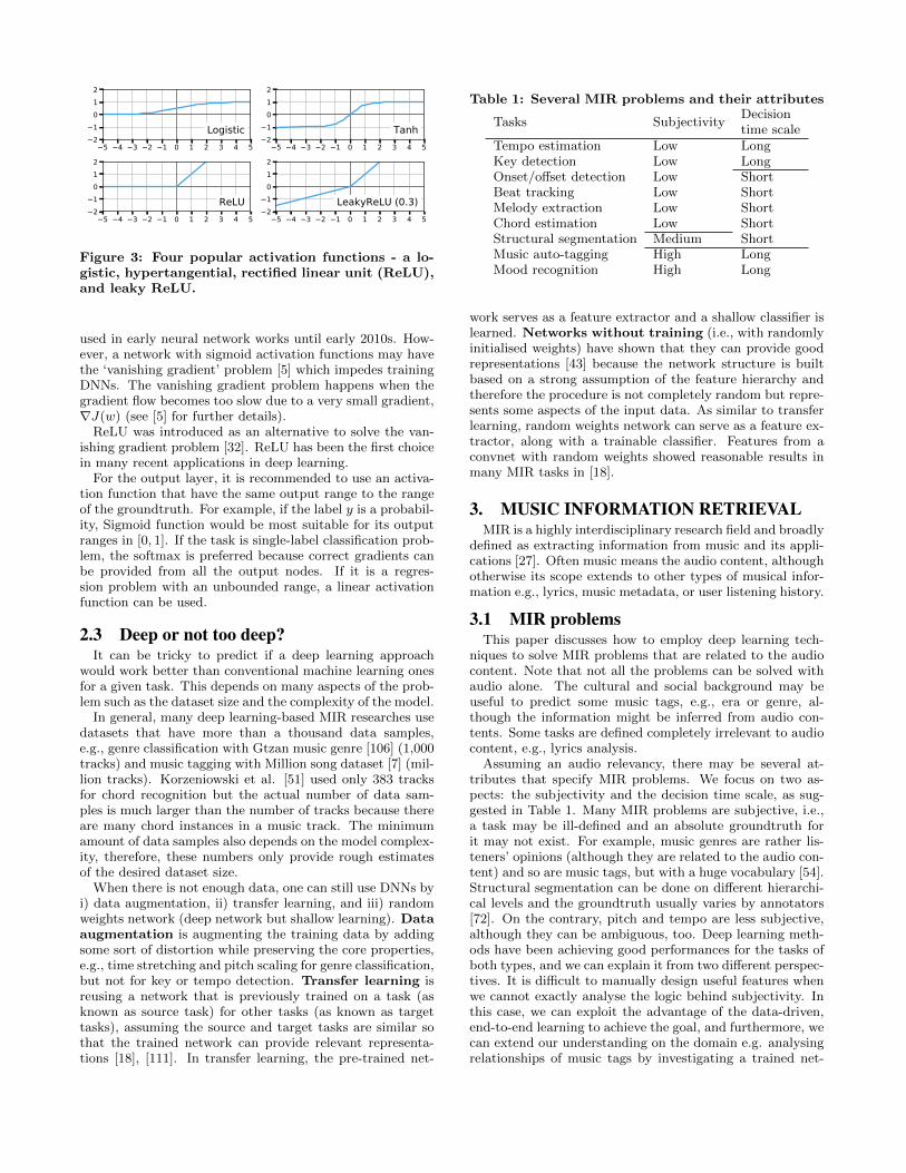
Figure 3: Four popular activation functions - a lo-gistic, hypertangential, rectified linear unit (ReLU),and leaky ReLU.

used in early neural network works until early 2010s. How-ever, a network with sigmoid activation functions may havethe ‘vanishing gradient’ problem [5] which impedes trainingDNNs. The vanishing gradient problem happens when thegradient flow becomes too slow due to a very small gradient,∇J(w) (see [5] for further details).

ReLU was introduced as an alternative to solve the van-ishing gradient problem [32]. ReLU has been the first choicein many recent applications in deep learning.

For the output layer, it is recommended to use an activa-tion function that have the same output range to the rangeof the groundtruth. For example, if the label y is a probabil-ity, Sigmoid function would be most suitable for its outputranges in [0, 1]. If the task is single-label classification prob-lem, the softmax is preferred because correct gradients canbe provided from all the output nodes. If it is a regres-sion problem with an unbounded range, a linear activationfunction can be used.

2.3 Deep or not too deep?It can be tricky to predict if a deep learning approach

would work better than conventional machine learning onesfor a given task. This depends on many aspects of the prob-lem such as the dataset size and the complexity of the model.

In general, many deep learning-based MIR researches usedatasets that have more than a thousand data samples,e.g., genre classification with Gtzan music genre [106] (1,000tracks) and music tagging with Million song dataset [7] (mil-lion tracks). Korzeniowski et al. [51] used only 383 tracksfor chord recognition but the actual number of data sam-ples is much larger than the number of tracks because thereare many chord instances in a music track. The minimumamount of data samples also depends on the model complex-ity, therefore, these numbers only provide rough estimatesof the desired dataset size.

When there is not enough data, one can still use DNNs byi) data augmentation, ii) transfer learning, and iii) randomweights network (deep network but shallow learning). Dataaugmentation is augmenting the training data by addingsome sort of distortion while preserving the core properties,e.g., time stretching and pitch scaling for genre classification,but not for key or tempo detection. Transfer learning isreusing a network that is previously trained on a task (asknown as source task) for other tasks (as known as targettasks), assuming the source and target tasks are similar sothat the trained network can provide relevant representa-tions [18], [111]. In transfer learning, the pre-trained net-

Table 1: Several MIR problems and their attributes

Tasks SubjectivityDecisiontime scale

Tempo estimation Low LongKey detection Low LongOnset/offset detection Low ShortBeat tracking Low ShortMelody extraction Low ShortChord estimation Low ShortStructural segmentation Medium ShortMusic auto-tagging High LongMood recognition High Long

work serves as a feature extractor and a shallow classifier islearned. Networks without training (i.e., with randomlyinitialised weights) have shown that they can provide goodrepresentations [43] because the network structure is builtbased on a strong assumption of the feature hierarchy andtherefore the procedure is not completely random but repre-sents some aspects of the input data. As similar to transferlearning, random weights network can serve as a feature ex-tractor, along with a trainable classifier. Features from aconvnet with random weights showed reasonable results inmany MIR tasks in [18].

3. MUSIC INFORMATION RETRIEVALMIR is a highly interdisciplinary research field and broadly

defined as extracting information from music and its appli-cations [27]. Often music means the audio content, althoughotherwise its scope extends to other types of musical infor-mation e.g., lyrics, music metadata, or user listening history.

3.1 MIR problemsThis paper discusses how to employ deep learning tech-

niques to solve MIR problems that are related to the audiocontent. Note that not all the problems can be solved withaudio alone. The cultural and social background may beuseful to predict some music tags, e.g., era or genre, al-though the information might be inferred from audio con-tents. Some tasks are defined completely irrelevant to audiocontent, e.g., lyrics analysis.

Assuming an audio relevancy, there may be several at-tributes that specify MIR problems. We focus on two as-pects: the subjectivity and the decision time scale, as sug-gested in Table 1. Many MIR problems are subjective, i.e.,a task may be ill-defined and an absolute groundtruth forit may not exist. For example, music genres are rather lis-teners’ opinions (although they are related to the audio con-tent) and so are music tags, but with a huge vocabulary [54].Structural segmentation can be done on different hierarchi-cal levels and the groundtruth usually varies by annotators[72]. On the contrary, pitch and tempo are less subjective,although they can be ambiguous, too. Deep learning meth-ods have been achieving good performances for the tasks ofboth types, and we can explain it from two different perspec-tives. It is difficult to manually design useful features whenwe cannot exactly analyse the logic behind subjectivity. Inthis case, we can exploit the advantage of the data-driven,end-to-end learning to achieve the goal, and furthermore, wecan extend our understanding on the domain e.g. analysingrelationships of music tags by investigating a trained net-

work [14]. Otherwise, if the logic is well-known, domainknowledge can help effectively structuring the network.

The other property of MIR problems that we focus on inthis paper is the decision time scale, which is the unit timelength based on which each prediction is made. For example,the tempo and the key are usually static in an excerpt if notin the whole track, which means tempo estimation and keydetection are of ‘long’ decision time scale, i.e., time-invariantproblems. On the other hand, a melody is often predicted oneach time frame which is usually in few tens of millisecond,therefore melody extraction is of ‘short’ decision time scale,i.e., a time-varying problem. Note that this is subject tochange depending on the way the problem is formulated.For example, music tagging is usually considered as a time-invariant problem but can be also a time-varying problem[115].

3.2 Audio data representationsIn this section, we review several audio data representa-

tions in the context of using deep learning methods. Ma-jorities of deep learning approaches in MIR take advantageof 2-dimensional representations instead of the original 1-dimensional representation which is the (discrete) audio sig-nal. In many cases, the two dimensions are frequency andtime axes.

When applying deep learning method to MIR problems,it is particularly important to understand the properties ofaudio data representations. Training DNNs is computation-ally intensive, therefore optimisation is necessary for everystage. One of the optimisations is to pre-process the inputdata so that it represents its information effectively and effi-ciently – effectively so that the network can easily use it andefficiently so that the memory usage and/or the computationis not too heavy.

In many cases, two-dimensional representations provideaudio data in an effective form. By decomposing the signalswith kernels of different centre frequencies (e.g., STFT), au-dio signals are separated, i.e., the information of the signalbecomes clearer.

Although those 2D representations have been consideredas visual images and these approaches have been workingwell, there are also differences. Visual images are locallycorrelated; nearby pixels are likely to have similar intensitiesand colours. In spectrograms, there are often harmonic cor-relations which are spread along frequency axis while localcorrelation may be weaker. [67] and [8] focus on the har-monic correlation by modifying existing 2D representations,which is out of the scope in this paper but strongly recom-mended to read. A scale invariance is expected for visualobject recognition but probably not for music/audio-relatedtasks.•Audio signal: The audio signal is often called raw au-

dio, compared to other representations that are transfor-mations based on it. A digital audio signal consists of audiosamples that specify the amplitudes at time-steps. In major-ity of MIR works, researchers assume that the music contentis given as a digital audio signal, isolating the task from theeffect of acoustic channels. The audio signal has not beenthe most popular choice; researchers have preferred 2D rep-resentations such as STFT and mel-spectrograms becauselearning a network starting from the audio signal requireseven a larger dataset.

Recently, however, one-dimensional convolutions are of-

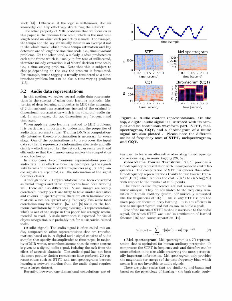
Figure 4: Audio content representations. On thetop, a digital audio signal is illustrated with its sam-ples and its continuous waveform part. STFT, mel-spectrogram, CQT, and a chromagram of a musicsignal are also plotted . Please note the differentscales of frequency axes of STFT, melspectrogram,and CQT.

ten used to learn an alternative of existing time-frequencyconversions, e.g., in music tagging [26, 59].•Short-Time Fourier Transform: STFT provides a

time-frequency representation with linearly-spaced centre fre-quencies. The computation of STFT is quicker than othertime-frequency representations thanks to fast Fourier trans-form (FFT) which reduces the cost O(N2) to O(N log(N))with respect to the number of FFT points.

The linear centre frequencies are not always desired inmusic analysis. They do not match to the frequency reso-lution of human auditory system, nor musically motivatedlike the frequencies of CQT. This is why STFT is not themost popular choice in deep learning – it is not efficient insize as melspectrogram and not as raw as audio signals.

One of the merits of STFT is that it invertible to the audiosignal, for which STFT was used in sonification of learnedfeatures [16] and source separation [44].

S(m,ω) =∞∑

n=−∞

x[n]w[n−m] exp−jωn (2)

•Mel-spectrogram: Mel-spectrogram is a 2D represen-tation that is optimised for human auditory perception. Itcompresses the STFT in frequency axis and therefore can bemore efficient in its size while preserving the most perceptu-ally important information. Mel-spectrogram only providesthe magnitude (or energy) of the time-frequency bins, whichmeans it is not invertible to audio signals.

There are other scales that are similar to mel-bands andbased on the psychology of hearing – the bark scale, equiv-

alent rectangular bandwidth (ERB), and gammatone filters[75]. They have not been compared in MIR context but inspeech research and the result did not show a significantdifference on mel/bark/ERB in speech synthesis [117] andmel/bark for speech recognition [94].

There are many suggestions on composing mel-frequencies.[76] suggests the formula as Eq. 3.

m = 2595 log10(1 +f

700) (3)

for frequency f in hertz. Trained kernels of end-to-endconfiguration have resulted in nonlinear frequencies that aresimilar to log-scale or mel-scale [26, 59]. Those results agreewith the known human perception [75] and indicate that themel-frequencies are quite suitable for the those tasks, per-haps because tagging is a subjective task. For those empir-ical and psychological reasons, mel-spectrograms have beenpopular for tagging [25] [15], [17], boundary detection [108],onset detection [90] and learning latent features of musicrecommendation [110].• Constant-Q Transform (CQT): CQT provides a 2D

representation with logarithmic-scale centre frequencies. Thisis well matched to the frequency distribution of the pitch,hence CQT has been predominantly used where the funda-mental frequencies of notes should be precisely identified,e.g. chord recognition [45] and transcription [96].The centrefrequencies are computed as Eq. 4.

fc(klf ) = fmin × 2klf/β (4)

, where fmin: minimum frequency of the analysis (Hz),klf : integer filter index, β : number of bins per octave, Z :number of octaves.

Note that the computation of a CQT is heavier than thatof an STFT or melspectrogram. (As an alternative, log-spectrograms can be used and showed even a better perfor-mance than CQT in piano transcription [49].)• Chromagram [4]: The chromagram, also often called

the pitch class profile, provides the energy distribution ona set of pitch classes, often with the western music’s 12pitches.[31] [114]. One can consider a chromagram as aCQT representation folding in the frequency axis. Givena log-frequency spectrum Xlf (e.g., CQT), it is computedas Eq. 5.

Cf (b) =

Z−1∑z=0

|Xlf (b+ zβ)| (5)

, where z=integer, octave index, b=integer, pitch classindex ∈ [0, β − 1].

Like MFCCs, chromagram is more ‘processed’ than otherrepresentations and can be used as a feature by itself.

4. DEEP NEURAL NETWORKS FOR MIRIn this section, we explain the layers that are frequently

used in deep learning. For each type of a layer, a generaloverview is followed by a further interpretation in the MIRcontext. Hereafter, we define symbols in layers as in Table2.

4.1 Dense layers

Symbols MeaningN Number of channels of a 2D representationF Frequency-axis length of a 2D representationT Time-axis length of a 2D representationH Height of a 2D convolution kernel (frequency-axis)W Width of a 2D convolution kernel (time-axis)V Number of hidden nodes of a layerL Number of layers of a network

Table 2: Symbols and their meanings defined in thispaper. Subscript indicates the layer index, e.g., N1

denotes the number of channels (feature maps) inthe first convolutional layer.

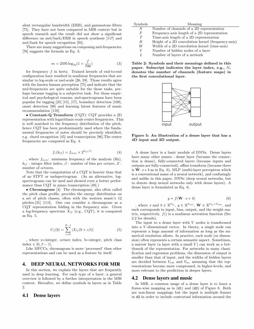
Figure 5: An illustration of a dense layer that has a4D input and 3D output.

A dense layer is a basic module of DNNs. Dense layershave many other names - dense layer (because the connec-tion is dense), fully-connected layers (because inputs andoutputs are fully-connected), affine transform (because thereis W ·x+b as in Eq. 6), MLP (multi-layer perceptron whichis a conventional name of a neural network), and confusinglyand unlike in this paper, DNNs (deep neural networks, butto denote deep neural networks only with dense layers). Adense layer is formulated as Eq. 6,

y = f(W · x + b) (6)

, where x and b ∈ RVin , y ∈ RVout , W ∈ RVin×Vout , andeach corresponds to input, bias, output, and the weight ma-trix, respectively. f() is a nonlinear activation function (Sec2.2 for details).

The input to a dense layer with V nodes is transformedinto a V -dimensional vector. In theory, a single node canrepresent a huge amount of information as long as the nu-merical resolution allows. In practice, each node (or dimen-sion) often represents a certain semantic aspect. Sometimes,a narrow layer (a layer with a small V ) can work as a bot-tleneck of the representation. For networks in many classi-fication and regression problems, the dimension of output issmaller than that of input, and the widths of hidden layersare decided between Vout and Vin, assuming that the rep-resentations become more compressed, in higher-levels, andmore relevant to the prediction in deeper layers.

4.2 Dense layers and musicIn MIR, a common usage of a dense layer is to learn a

frame-wise mapping as in (d1) and (d2) of Figure 8. Bothare non-linear mappings but the input is multiple framesin d2 in order to include contextual information around the

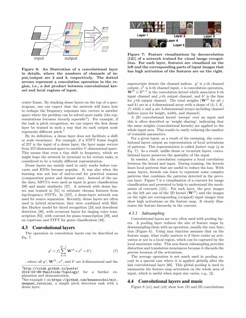
Figure 6: An illustration of a convolutional layerin details, where the numbers of channels of in-put/output are 2 and 3, respectively. The dottedarrows represent a convolution operation in the re-gion, i.e., a dot product between convolutional ker-nel and local regions of input.

centre frame. By stacking dense layers on the top of a spec-trogram, one can expect that the network will learn howto reshape the frequency responses into vectors in anotherspace where the problem can be solved more easily (the rep-resentations becomes linearly separable3). For example, ifthe task is pitch recognition, we can expect the first denselayer be trained in such a way that its each output noderepresents different pitch.4

By its definition, a dense layer does not facilitate a shiftor scale invariance. For example, if a STFT frame lengthof 257 is the input of a dense layer, the layer maps vectorsfrom 257-dimensional space to another V -dimensional space.This means that even a tiny shift in frequency, which wemight hope the network be invariant to for certain tasks, isconsidered to be a totally different representation.

Dense layers are mainly used in early works before con-vnets and RNNs became popular. It was also when thelearning was not less of end-to-end for practical reasons(computation power and dataset size). Instead of the au-dio data, MFCCs were used as input in genre classification[98] and music similarity [37]. A network with dense lay-ers was trained in [51] to estimate chroma features fromlog-frequency STFTs. In [107], a dense-layer network wasused for source separation. Recently, dense layers are oftenused in hybrid structures; they were combined with Hid-den Markov model for chord recognition [24] and downbeatdetection [28], with recurrent layers for singing voice tran-scription [82], with convnet for piano transcription [49], andon cepstrum and STFT for genre classification [48].

4.3 Convolutional layersThe operation in convolution layers can be described as

Eq. 7.

yj = f(

K−1∑k=0

Wjk ∗ xk + bj) (7)

, where all yj , Wjk, xk, and bj are 2-dimensional and the

3http://colah.github.io/posts/2014-03-NN-Manifolds-Topology/ for a further ex-planation and demonstration.4See example 1 on https://github.com/keunwoochoi/mir_deepnet_tutorial, a simple pitch detection task with adense layer.

Figure 7: Feature visualisations by deconvolution[121] of a network trained for visual image recogni-tion. For each layer, features are visualised on theleft and the corresponding parts of input images thathas high activation of the features are on the right.

superscripts denote the channel indices. yj is j-th channeloutput, xk is k-th channel input, ∗ is convolution operation,Wjk ∈ Rh×l is the convolution kernel which associates k-thinput channel and j-th output channel, and bj is the biasfor j-th output channel. The total weights (Wjk for all jand k) are in a 4-dimensional array with a shape of (h, l, K,J) while x and y are 3-dimensional arrays including channelindices (axes for height, width, and channel).

A 2D convolutional kernel ‘sweeps’ over an input andthis is often described as ‘weight sharing’, indicating thatthe same weights (convolutional kernels) are applied to thewhole input area. This results in vastly reducing the numberof trainable parameters.

For a given input, as a result of the sweeping, the convo-lutional layers output an representation of local activationsof patterns. This representation is called feature map (y inEq. 7). As a result, unlike dense or recurrent layers, convo-lutional layers preserves the spatiality of the input.

In essence, the convolution computes a local correlationbetween the kernel and input. During training, the kernelslearn local patterns that are useful to reduce the loss. Withmany layers, kernels can learn to represent some complexpatterns that combines the patterns detected in the previ-ous layer. Figure 7 is a visualisation of a convnet for imageclassification and presented to help to understand the mech-anism of convnets [121]. For each layer, the grey imageson the left are one of the 2D kernel (Wjk) and the imageson the right are corresponding (cropped) input images thatshow high activations on the feature map. It clearly illus-trates the feature hierarchy in the convnet.

4.3.1 SubsamplingConvolutional layers are very often used with pooling lay-

ers. A pooling layer reduces the size of feature maps bydownsampling them with an operation, usually the max func-tion (Figure 6). Using max function assumes that on thefeature maps, what really matters is if there exists an acti-vation or not in a local region, which can be captured by thelocal maximum value. This non-linear subsampling providesdistortion and translation invariances because it discards theprecise location of the activations.

The average operation is not much used in pooling ex-cept in a special case where it is applied globally after thelast convolutional layer [66]. This global pooling is used tosummarise the feature map activation on the whole area ofinput, which is useful when input size varies, e.g., [2].

4.4 Convolutional layers and musicFigure 8 (c1) and (c2) show how 1D and 2D convolutions

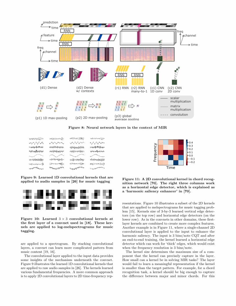
Figure 8: Neural network layers in the context of MIR

Figure 9: Learned 1D convolutional kernels that areapplied to audio samples in [26] for music tagging

Figure 10: Learned 3 × 3 convolutional kernels atthe first layer of a convnet used in [18]. These ker-nels are applied to log-melspectrograms for musictagging.

are applied to a spectrogram. By stacking convolutionallayers, a convnet can learn more complicated pattern frommusic content [19, 16].

The convolutional layer applied to the input data providessome insights of the mechanism underneath the convnet.Figure 9 illustrates the learned 1D convolutional kernels thatare applied to raw audio samples in [26]. The kernels learnedvarious fundamental frequencies. A more common approachis to apply 2D convolutional layers to 2D time-frequency rep-

Time

Freq

uenc

y0.20.1

0.00.10.20.30.4

Figure 11: A 2D convolutional kernel in chord recog-nition network [70]. The right three columns workas a horizontal edge detector, which is explained asa ‘harmonic saliency enhancer’ in [70].

resentations. Figure 10 illustrates a subset of the 2D kernelsthat are applied to melspectrograms for music tagging prob-lem [15]. Kernels size of 3-by-3 learned vertical edge detec-tors (on the top row) and horizontal edge detectors (on thelower row). As in the convnets in other domains, these first-layer kernels are combined to create more complex features.Another example is in Figure 11, where a single-channel 2Dconvolutional layer is applied to the input to enhance theharmonic saliency. The input is 3 bins/note CQT and afteran end-to-end training, the kernel learned a horizontal edgedetector which can work for ‘thick’ edges, which would existwhen the frequency resolution is 3 bins/note.

The kernel size determines the maximum size of a com-ponent that the kernel can precisely capture in the layer.How small can a kernel be in solving MIR tasks? The layerwould fail to learn a meaningful representation if the kernelis smaller than the target pattern. For example, for a chordrecognition task, a kernel should be big enough to capturethe difference between major and minor chords. For this

reason, relatively large-sized kernels such as 17× 5 are usedon 36-bins/octave CQT in [45]. A special case is to use dif-ferent shapes of kernels in the same layer as in the Inceptionmodule [104] which is used for hit song prediction in [118].

The second question would be then how big can a kernelbe? One should note that a kernel does not allow an in-variance within it. Therefore, if a large target pattern mayslightly vary inside, it would better be captured with stackedconvolutional layers with subsamplings so that small distor-tions can be allowed. More discussions on the kernel shapesfor MIR research are available in [80, 79].

Max-pooling is frequently used in MIR to add time/frequencyinvariant. Such a subsampling is necessary in the DNNs fortime-invariant problems in order to yield a one, single pre-diction for the whole input. In this case, One can begin withspecifying the size of target output, followed by deciding de-tails of poolings (how many and how much in each stage)somehow empirically.

A special use-case of the convolutional layer is to use 1Dconvolutional layers directly onto an audio signal (which isoften referred as a raw input) to learn the time-frequencyconversions in [26], and furthermore, [60]. This approach isalso proposed in speech/audio and resulted in similar kernelslearned of which fundamental frequencies are similar to log-or mel-scale frequencies [85]. Figure 9 illustrates a subset oftrained kernel in [26]. Note that unlike STFT kernels, theyare not pure sinusoid and include harmonic components.

The convolutional layer has been very popular in MIR. Apioneering convnet research for MIR is convolutional deepbelief networks for genre classification [58]. Early works re-lied on MFCC input to reduce computation [62], [63] forgenre classification. Many works have been then introducedbased on time-frequency representations e.g., CQT for chordrecognition [45], guitar chord recognition [46], genre classifi-cation [116], transcription [96], melspectrogram for bound-ary detection [89], onset detection [90], hit song prediction[118], similarity learning [68], instrument recognition [39],music tagging [26], [15], [17], [59], and STFT for boundarydetection [36], vocal separation [100], and vocal detection[88]. One-dimensional CNN for raw audio input is used formusic tagging [26], [60], synthesising singing voice [9], poly-phonic music [112], and instruments [29].

4.5 Recurrent layersA recurrent layer incorporates a recurrent connection and

is formulated as Eq. 8.

yt = fout(Vht)

ht = fh(Uxt + Wht−1)(8)

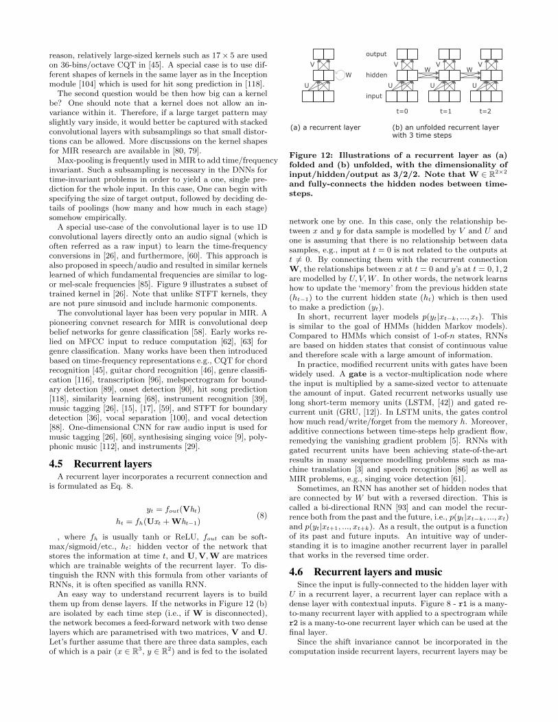
, where fh is usually tanh or ReLU, fout can be soft-max/sigmoid/etc., ht: hidden vector of the network thatstores the information at time t, and U,V,W are matriceswhich are trainable weights of the recurrent layer. To dis-tinguish the RNN with this formula from other variants ofRNNs, it is often specified as vanilla RNN.

An easy way to understand recurrent layers is to buildthem up from dense layers. If the networks in Figure 12 (b)are isolated by each time step (i.e., if W is disconnected),the network becomes a feed-forward network with two denselayers which are parametrised with two matrices, V and U.Let’s further assume that there are three data samples, eachof which is a pair (x ∈ R3, y ∈ R2) and is fed to the isolated

Figure 12: Illustrations of a recurrent layer as (a)folded and (b) unfolded, with the dimensionality ofinput/hidden/output as 3/2/2. Note that W ∈ R2×2

and fully-connects the hidden nodes between time-steps.

network one by one. In this case, only the relationship be-tween x and y for data sample is modelled by V and U andone is assuming that there is no relationship between datasamples, e.g., input at t = 0 is not related to the outputs att 6= 0. By connecting them with the recurrent connectionW, the relationships between x at t = 0 and y’s at t = 0, 1, 2are modelled by U, V,W . In other words, the network learnshow to update the ‘memory’ from the previous hidden state(ht−1) to the current hidden state (ht) which is then usedto make a prediction (yt).

In short, recurrent layer models p(yt|xt−k, ..., xt). Thisis similar to the goal of HMMs (hidden Markov models).Compared to HMMs which consist of 1-of-n states, RNNsare based on hidden states that consist of continuous valueand therefore scale with a large amount of information.

In practice, modified recurrent units with gates have beenwidely used. A gate is a vector-multiplication node wherethe input is multiplied by a same-sized vector to attenuatethe amount of input. Gated recurrent networks usually uselong short-term memory units (LSTM, [42]) and gated re-current unit (GRU, [12]). In LSTM units, the gates controlhow much read/write/forget from the memory h. Moreover,additive connections between time-steps help gradient flow,remedying the vanishing gradient problem [5]. RNNs withgated recurrent units have been achieving state-of-the-artresults in many sequence modelling problems such as ma-chine translation [3] and speech recognition [86] as well asMIR problems, e.g., singing voice detection [61].

Sometimes, an RNN has another set of hidden nodes thatare connected by W but with a reversed direction. This iscalled a bi-directional RNN [93] and can model the recur-rence both from the past and the future, i.e., p(yt|xt−k, ..., xt)and p(yt|xt+1, ..., xt+k). As a result, the output is a functionof its past and future inputs. An intuitive way of under-standing it is to imagine another recurrent layer in parallelthat works in the reversed time order.

4.6 Recurrent layers and musicSince the input is fully-connected to the hidden layer with

U in a recurrent layer, a recurrent layer can replace with adense layer with contextual inputs. Figure 8 - r1 is a many-to-many recurrent layer with applied to a spectrogram whiler2 is a many-to-one recurrent layer which can be used at thefinal layer.

Since the shift invariance cannot be incorporated in thecomputation inside recurrent layers, recurrent layers may be

suitable for the sequences of features. The features can beeither known music and audio features such as MFCCs orfeature maps from convolutional layers [17].

All the inputs are sequentially transformed and summedto a V -dimensional vector, therefore it should be capable ofcontaining enough information. The size, V , is one of thehyperparameter and choosing it involves many trials andcomparison. Its initial value can be estimated by consider-ing the dimensionality of input and output. For example,V can be between their sizes, assuming the network learnsto compress the input while preserving the information tomodel the output.

One may want to control the length of a recurrent layer tooptimise the computational cost. For example, on the onsetdetection problem, probably only a few context frames canbe used since onsets can be specified in a very short time,while chord recognition may benefit from longer inputs.

Many time-varying MIR problems are time-aligned, i.e.,the groundtruth exists for a regular rate and the problemdoes not require sequence matching techniques such as dy-namic time warping. This formulation makes it suitable tosimply apply ‘many-to-many’ recurrent layer (Figure 8 - r1).On the other hand, classification problems such as genre ortag only have one output prediction. For those problems, the‘many-to-one’ recurrent layer (Figure 8 - r2) can be used toyield only one output prediction at the final time step. Moredetails are in Section 5.2

For many MIR problems, inputs from the future can helpthe prediction and therefore bi-directional setting is worthtrying. For example, onsets can be effectively captured withaudio contents before and after the onsets, and so are off-sets/segment boundaries/beats.

So far, recurrent layers have been mainly used for time-varying prediction; for example, singing voice detection [61],singing and instrument transcription [82], [96] [95], and emo-tion prediction [64]. For time-invariant tasks, a music tag-ging algorithm used a hybrid structure of convolutional andrecurrent layers [17].

5. SOLVING MIR PROBLEMS: PRACTICALADVICE

In this section, we focus on more practical advice by pre-senting examples/suggestions of deep neural network modelsas well as discussing several practical issues.

5.1 Data preprocessingPreprocessing input data is very important to effectively

train neural networks. One may argue that the neural net-works can learn any types of preprocessing. However, addingtrainable parameters always requires more training data,and some preprocessing such as standardisation substan-tially effects the training speed [57].

Furthermore, audio data requires some designated prepro-cessing steps. When using the magnitudes of 2D representa-tions, logarithmic mapping of magnitudes (X→ log(X+ ε))is widely used to condition the data distributions and oftenresults in better performance [13]. Besides, preprocessingaudio data is an open issue yet. Spectral whitening can beused to compensate the different energy level by frequencies[97]. However, it did not improve the performance on musictagging convnet [13]. With 2D convnet, it seems not helpfulto normalise local contrasts in computer vision, which may

be applicable for convnet in MIR as well.Lastly, one may want to optimise the signal processing

parameters such as the numbers of FFT and mel-bins, win-dow and hop sizes, and the sampling rate. As explained inSection 3.2, it is important to minimise the data size foran efficient training. To reduce the data size, audio signalsare often downmixed and downsampled to 8-16kHz. Afterthen, one can try real-time preprocessing with utilities suchas Kapre [20], Pescador5, Fuel[113], Muda [71], otherwisepre-computing and storing can be an issue in practice.

5.2 Aggregating informationThe time-varying/time-invariant problems need different

network structures. As in Table 1, problems with a shortdecision time scale, or time-varying problems, require a pre-diction per unit time, often per short time frame. On thecontrary, for problems with a long decision time scale, thereshould be a method implemented to aggregate the featuresover time. Frequently used methods are i) pooling, ii) stridedconvolutions, and iii) recurrent layers with many-to-one con-figuration.

i) Pooling: With convolutional layers, a very commonmethod is to use max-pooling layers(s) over time (and oftenas well as frequency) axis (also discussed in Section 4.3.1).A special case is to use a global pooling after the last con-volutional layer [66] as in Figure 8.

ii) Strided convolutions: Strided convolutions are theoperations of convolutional layers that have strides largerthan 1. The effects of this are known to be similar to max-pooling, especially under the generic and simple supervisedlearning structures that are introduced in this paper. Oneshould be careful to set the strides to be smaller than theconvolutional kernel sizes so that all part of the input isconvolved.

iii) Recurrent layers: Recurrent layers can learn tosummarise features in any axis. They involve trainable pa-rameters and therefore take more computation and data todo the job than the previous two approaches. The previoustwo can reduce the size gradually, but recurrent layers areoften set to many-to-one. Therefore, it was used in the lastlayer rather than intermediate layers in [17].

5.3 Depth of networksIn designing a network, one may find it arbitrary and em-

pirical to decide the depth of the network. The networkshould be deep enough to approximate the relationship be-tween the input and the output. If the relationship can be(roughly) formulated, one can start with a depth with whichthe network can implement the formula. Fortunately, it isbecoming easier to train a very deep network [101, 41, 40].

For convnets, the depth is increasing in MIR as well asother domains. For example, networks for music tagging,boundary detection, and chord recognition in 2014 used 2-layer convnet [26], [90], [46], but recent research often uses5 or more convolutional layers [15, 68, 52].

The depth of RNNs has been increasing slowly. This isa general trend including MIR and may because i) stackingrecurrent layers does not incorporate feature hierarchy andii) a recurrent layer already are deep due to the recurrentconnection, i.e., it is deep along the time axis, therefore thenumber of layers is less critical than that of convnets.

5http://pescador.readthedocs.io

5.4 First layer to input

• d1: As mentioned earlier, dense layers are not fre-quency shift invariant. In the output, dense layers re-move the spatiality along frequency axis because thewhole frequency range is mapped into scalar values.

• d2: The operation, a matrix multiplication to input,is the same as d1 but it is performed with multipleframes as an input.

• c1: With F -by-1 convolution kernels, the operation isequivalent to d1. F -by-W kernels with W > 1 are alsoequivalent to d2.

• c2: Many recent DNN structures use a 2-dimensionalconvolutional layer to the spectrogram inputs. Thelayer outputs N feature maps which preserve the spa-tiality on both axes.

A special usage of a 2D convolutional layer is to use itas a preprocessing layer, hoping to enhance the saliencyof some pattern as in [70], where 5×5 kernels compressthe transient for a better chord recognition. Depend-ing on the task, it can also enhance the transient [16]or do the both – to approximate a harmonic-percussiveseparation.

• r1: It maps input frames to another dimension, whichis same as d1. Since recurrent layer can take manynearby frames, the assumption of using r1 is very sim-ilar to that of d2.

5.5 Intermediate layers

• d1, d2, c1, r1 : Repeating these layers adds more non-linearity to the model.

Note that Stacking layers with context enables the net-work to ‘look’ even wider contexts. For example, imag-ine dense layers, both are taking adjacent 4 frames (2from the past and 2 from the future), then y2[t], theoutput of the second layer, is a function of x2[t − 2 :t + 2] = y1[t − 2 : t + 2], which is a function ofx1[t− 4 : t+ 4].

• c2: Many structures consist of more than one convo-lutional layers. As in the case above, stacking convo-lutional layers also enables the network to look largerrange.

• p1, p2: A pooling layer often follows convolutionallayers as mentioned in Section 4.3.1.

5.6 Output layersDense layers are almost always used in the output layer,

where the number of node V is set to the number of classes inclassification problem or the dimensionality of the predictedvalues in the regression problem. For example, if the taskis to classify the music into 10 genres, a dense layer with10 nodes (with a softmax activation function) can be usedwhere each node represents a probability for each genre andthe groundtruth is given as one-hot-vector.

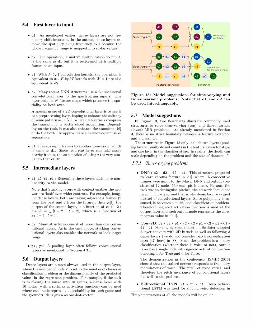
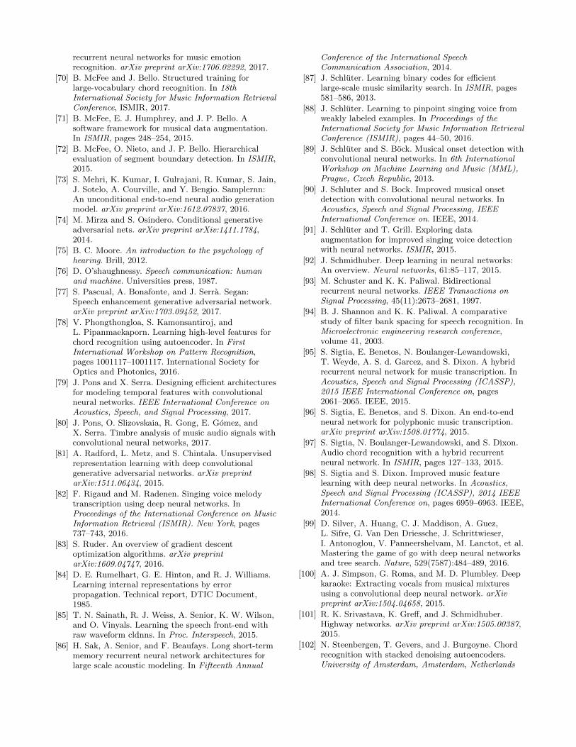
Figure 13: Model suggestions for time-varying andtime-invariant problems. Note that d1 and d2 canbe used interchangeably.

5.7 Model suggestionsIn Figure 13, two flowcharts illustrate commonly used

structures to solve time-varying (top) and time-invariant(lower) MIR problems. As already mentioned in Section4, there is no strict boundary between a feature extractorand a classifier.

The structures in Figure 13 only include two layers (pool-ing layers usually do not count) in the feature extractor stageand one layer in the classifier stage. In reality, the depth canscale depending on the problem and the size of datasets. 6

5.7.1 Time-varying problems

• DNN: d2 - d2 - d2 - d1: This structure proposedto learn chroma feature in [51], where 15 consecutiveframes were input to the 3-layer DNN and output con-sisted of 12 nodes (for each pitch class). Because thetask was to distinguish pitches, the network should notbe pitch invariant, and that is why dense layer was usedinstead of convolutional layers. Since polyphony is as-sumed, it becomes a multi-label classification problem.Therefore, sigmoid activation function is used at theoutput layer and each output node represents the chro-magram value in [0, 1].

• Conv2D: c2 - c2 - p1 - c2 - c2 - p1 - c2 - p1 - d1 -d1 - d1: For singing voice detection, Schluter adopted5-layer convnet with 2D kernels as well as following 3dense layers (we do not consider batch normalizationlayer [47] here) in [88]. Since the problem is a binaryclassification (whether there is voice or not), outputlayer has a single node with sigmoid activation functiondenoting 1 for True and 0 for False.

The demonstration in the conference (ISMIR 2016)showed that the trained network responds to frequencymodulations of voice. The pitch of voice varies, andtherefore the pitch invariance of convolutional layersfits well to the problem.

• Bidirectional RNN: r1 - r1 - d1: Deep bidirec-tional LSTM was used for singing voice detection in

6Implementations of all the models will be online.

[61]. The depth affected the performance and 4-layernetwork achieved the best performance among [2, 3,4, 5]-layer architectures. Although [61] did not com-pare the result without a bi-directional configuration,we can guess it probably helped, because the vocal ex-istence at time t is probably not independent of theadjacent frames.

In [61], the preprocessing stage includes harmonic-percussiveseparation [105] to enhance the vocal melody. One canadd other preprocessing steps that are relevant to thetask, although it is not very common in practice dueto a heavy computation.

5.7.2 Time-invariant problems

• Conv1d: c1 - p1 - c1 - p1 - d1 - d1 - d1

The 1D convolution at the first layer reduces the sizedrastically (F × T → 1 × T , since the height of con-volutional kernel is same as F ). Therefore, this modelis computational efficient [17]. It is one of the earlystructures that were used in MIR, e.g., music tagging[26]. Note that the pooling is performed only alongtime axis because feature-axis does not imply any spa-tial meaning.

The limit of this model comes from the large kernelsize; since convolutional layers do not allow varianceswithin the kernels, the layer is not able to learn localpatterns (‘local’ in frequency axis).

• Conv2d: c2 - p2 - c2 - p2 - c2 - p2 - d2: Bystacking 2D convolutions and subsamplings, the net-work can see the input spectrograms at different scales.The early layers learns relevant local patterns, which iscombined in the deeper layers. As a result, the networkcovers the whole input range with small distortions al-lowed.

Convnets with 2D convolutions have been used in manyclassification and regression tasks including music tag-ging [15], onset detection [90], boundary detection [108],and singing voice detection [88].

• CRNN: c2 - p2 - c2 - p2 - r1 - r2 - d1

This structure combines convolutional and recurrentlayers [17]. The early convolutional layers capture localpatterns and pooling layers reduce the size to someextent. At the end, the recurrent layer summarise thefeature maps.

The benchmark in [17] showed that the network bene-fit from the flexibility of recurrent layers in summaris-ing information along time, achieving the best perfor-mance among the structures. CRNN was also used inmusic emotion recognition and achieved state-of-the-art performance [69].

6. CONCLUSIONSIn this paper, we presented a tutorial on deep learning

for MIR research. Using deep learning to solve a problemis more than simply loading the data and feed it to thenetwork. Due to heavy computation, exhaustive search forthe hyperparameters of a network is not a viable option,

therefore one should carefully decide the structure with un-derstanding both the domain knowledge and deep learningtechniques.

We reviewed the basics of deep learning – what is deeplearning and designing a structure, how to train it, andwhen to use deep learning. We also reviewed MIR, focusingon the essential aspects for using deep learning. Then wesummarised three popular layers - dense, convolutional, andrecurrent layers as well as their interpretations in the MIRcontext. Based on the understanding of the layers, one candesign a new network structure for a specific task. Finally,we summarised more practical aspects of using deep learningfor MIR including popular structures with their properties.Although the structures were proposed to a certain problem,they can be broadly used for other problems as well.

Deep learning has achieved many state-of-the-art resultsin various domains and even surpassing human level in sometasks such as image recognition [41] or playing games [99].We strongly believe that there still is a great potential fordeep learning and there will be even more MIR researchrelying on deep learning methods.

AcknowledgementsThis work has been part funded by FAST IMPACt EPSRCGrant EP/L019981/1 and the European Commission H2020research and innovation grant AudioCommons (688382). MarkSandler acknowledges the support of the Royal Society as arecipient of a Wolfson Research Merit Award. KyunghyunCho thanks the support by eBay, TenCent, Facebook, Googleand NVIDIA.

We appreciate Adib Mehrabi, Beici Liang, Delia Fanoyela,Blair Kaneshiro, and Sertan Senturk for their helpful com-ments on writing this paper.

7. REFERENCES[1] M. Arjovsky, S. Chintala, and L. Bottou. Wasserstein

gan. arXiv preprint arXiv:1701.07875, 2017.

[2] Y. Aytar, C. Vondrick, and A. Torralba. Soundnet:Learning sound representations from unlabeled video.In Advances in Neural Information ProcessingSystems, pages 892–900, 2016.

[3] D. Bahdanau, K. Cho, and Y. Bengio. Neuralmachine translation by jointly learning to align andtranslate. In ICLR 2015, 2014.

[4] J. P. Bello. Chroma and tonality. Music InformationRetrieval Course.

[5] Y. Bengio, P. Simard, and P. Frasconi. Learninglong-term dependencies with gradient descent isdifficult. IEEE transactions on neural networks,5(2):157–166, 1994.

[6] D. Berthelot, T. Schumm, and L. Metz. Began:Boundary equilibrium generative adversarialnetworks. arXiv preprint arXiv:1703.10717, 2017.

[7] T. Bertin-Mahieux, D. P. Ellis, B. Whitman, andP. Lamere. The million song dataset. In ISMIR 2011:Proceedings of the 12th International Society forMusic Information Retrieval Conference, October24-28, 2011, Miami, Florida, pages 591–596.University of Miami, 2011.

[8] R. Bittner, B. McFee, J. Salamon, P. Li, and J. Bello.Deep salience representations for f0 estimation inpolyphonic music. In 18th International Society for

Music Information Retrieval Conference, ISMIR,2017.

[9] M. Blaauw and J. Bonada. A neural parametricsinging synthesizer. arXiv preprint arXiv:1704.03809,2017.

[10] S. Bock, F. Krebs, and G. Widmer. Accurate tempoestimation based on recurrent neural networks andresonating comb filters. In ISMIR, pages 625–631,2015.

[11] L. Chen, S. Srivastava, Z. Duan, and C. Xu. Deepcross-modal audio-visual generation. arXiv preprintarXiv:1704.08292, 2017.

[12] K. Cho, B. van Merrienboer, C. Gulcehre,F. Bougares, H. Schwenk, and Y. Bengio. Learningphrase representations using rnn encoder-decoder forstatistical machine translation. In Conference onEmpirical Methods in Natural Language Processing(EMNLP 2014), 2014.

[13] K. Choi, G. Fazekas, K. Cho, and M. Sandler. Acomparison on audio signal preprocessing methodsfor deep neural networks on music tagging.arXiv:1709.01922, 2017.

[14] K. Choi, G. Fazekas, K. Cho, and M. Sandler. Theeffects of noisy labels on deep convolutional neuralnetworks for music classification. arXiv:1706.02361,2017.

[15] K. Choi, G. Fazekas, and M. Sandler. Automatictagging using deep convolutional neural networks. InThe 17th International Society of Music InformationRetrieval Conference, New York, USA. InternationalSociety of Music Information Retrieval, 2016.

[16] K. Choi, G. Fazekas, and M. Sandler. Explainingdeep convolutional neural networks on musicclassification. arXiv preprint arXiv:1607.02444, 2016.

[17] K. Choi, G. Fazekas, M. Sandler, and K. Cho.Convolutional recurrent neural networks for musicclassification. In 2017 IEEE International Conferenceon Acoustics, Speech, and Signal Processing, 2016.

[18] K. Choi, G. Fazekas, M. Sandler, and K. Cho.Transfer learning for music classification andregression tasks. In The 18th International Society ofMusic Information Retrieval (ISMIR) Conference2017, Suzhou, China. International Society of MusicInformation Retrieval, 2017.

[19] K. Choi, G. Fazekas, M. Sandler, and J. Kim.Auralisation of deep convolutional neural networks:Listening to learned features. ISMIR late-breakingsession, 2015.

[20] K. Choi, D. Joo, and J. Kim. Kapre: On-gpu audiopreprocessing layers for a quick implementation ofdeep neural network models with keras. In MachineLearning for Music Discovery Workshop at 34thInternational Conference on Machine Learning.ICML, 2017.

[21] Y.-A. Chung, C.-C. Wu, C.-H. Shen, H.-Y. Lee, andL.-S. Lee. Audio word2vec: Unsupervised learning ofaudio segment representations usingsequence-to-sequence autoencoder. arXiv preprintarXiv:1603.00982, 2016.

[22] G. E. Dahl, T. N. Sainath, and G. E. Hinton.Improving deep neural networks for lvcsr usingrectified linear units and dropout. In Acoustics,

Speech and Signal Processing (ICASSP), 2013 IEEEInternational Conference on, pages 8609–8613. IEEE,2013.

[23] M. Defferrard. Structured auto-encoder withapplication to music genre recognition. Technicalreport, 2015.

[24] J. Deng and Y.-K. Kwok. Automatic chordestimation on seventhsbass chord vocabulary usingdeep neural network. In Acoustics, Speech and SignalProcessing (ICASSP), 2016 IEEE InternationalConference on, pages 261–265. IEEE, 2016.

[25] S. Dieleman and B. Schrauwen. Multiscaleapproaches to music audio feature learning. InISMIR, pages 3–8, 2013.

[26] S. Dieleman and B. Schrauwen. End-to-end learningfor music audio. In Acoustics, Speech and SignalProcessing (ICASSP), 2014 IEEE InternationalConference on, pages 6964–6968. IEEE, 2014.

[27] J. S. Downie. Music information retrieval. Annualreview of information science and technology,37(1):295–340, 2003.

[28] S. Durand, J. P. Bello, B. David, and G. Richard.Downbeat tracking with multiple features and deepneural networks. In Acoustics, Speech and SignalProcessing (ICASSP), 2015 IEEE InternationalConference on, pages 409–413. IEEE, 2015.

[29] J. Engel, C. Resnick, A. Roberts, S. Dieleman,D. Eck, K. Simonyan, and M. Norouzi. Neural audiosynthesis of musical notes with wavenetautoencoders. arXiv preprint arXiv:1704.01279, 2017.

[30] F. Eyben, S. Bock, B. W. Schuller, and A. Graves.Universal onset detection with bidirectional longshort-term memory neural networks. In Ismir, pages589–594, 2010.

[31] T. Fujishima. Realtime chord recognition of musicalsound: a system using common lisp music. In ICMC,pages 464–467, 1999.

[32] X. Glorot, A. Bordes, and Y. Bengio. Deep sparserectifier neural networks. In Aistats, volume 15, page275, 2011.

[33] Y. Goldberg. A primer on neural network models fornatural language processing. J. Artif. Intell.Res.(JAIR), 57:345–420, 2016.

[34] I. Goodfellow, Y. Bengio, and A. Courville. Deeplearning. MIT press, 2016.

[35] I. Goodfellow, J. Pouget-Abadie, M. Mirza, B. Xu,D. Warde-Farley, S. Ozair, A. Courville, andY. Bengio. Generative adversarial nets. In Advancesin neural information processing systems, pages2672–2680, 2014.

[36] T. Grill and J. Schluter. Music boundary detectionusing neural networks on spectrograms andself-similarity lag matrices. In Proceedings of the 23rdEuropean Signal Processing Conference (EUSPICO2015), Nice, France, 2015.

[37] P. Hamel, M. E. Davies, K. Yoshii, and M. Goto.Transfer learning in mir: Sharing learned latentrepresentations for music audio classification andsimilarity. 14th International Conference on MusicInformation Retrieval, 2013.

[38] P. Hamel and D. Eck. Learning features from music

audio with deep belief networks. In ISMIR, pages339–344. Utrecht, The Netherlands, 2010.

[39] Y. Han, J. Kim, and K. Lee. Deep convolutionalneural networks for predominant instrumentrecognition in polyphonic music. IEEE/ACMTransactions on Audio, Speech, and LanguageProcessing, 25(1):208–221, 2017.

[40] K. He, X. Zhang, S. Ren, and J. Sun. Delving deepinto rectifiers: Surpassing human-level performanceon imagenet classification. In Proceedings of theIEEE international conference on computer vision,pages 1026–1034, 2015.

[41] K. He, X. Zhang, S. Ren, and J. Sun. Deep residuallearning for image recognition. In Proceedings of theIEEE Conference on Computer Vision and PatternRecognition, pages 770–778, 2016.

[42] S. Hochreiter and J. Schmidhuber. Long short-termmemory. Neural computation, 9(8):1735–1780, 1997.

[43] G.-B. Huang, Q.-Y. Zhu, and C.-K. Siew. Extremelearning machine: a new learning scheme offeedforward neural networks. In Neural Networks,2004. Proceedings. 2004 IEEE International JointConference on, volume 2, pages 985–990. IEEE, 2004.

[44] P.-S. Huang, M. Kim, M. Hasegawa-Johnson, andP. Smaragdis. Singing-voice separation frommonaural recordings using deep recurrent neuralnetworks. In ISMIR, pages 477–482, 2014.

[45] E. J. Humphrey and J. P. Bello. Rethinkingautomatic chord recognition with convolutionalneural networks. In Machine Learning andApplications, 11th International Conference on,volume 2, pages 357–362. IEEE, 2012.

[46] E. J. Humphrey and J. P. Bello. From music audio tochord tablature: Teaching deep convolutionalnetworks toplay guitar. In Acoustics, Speech andSignal Processing, IEEE International Conferenceon, pages 6974–6978. IEEE, 2014.

[47] S. Ioffe and C. Szegedy. Batch normalization:Accelerating deep network training by reducinginternal covariate shift. arXiv preprintarXiv:1502.03167, 2015.

[48] I.-Y. Jeong and K. Lee. Learning temporal featuresusing a deep neural network and its application tomusic genre classification. Proc. of the 17th Int.Society for Music Information RetrievalConf.(ISMIR), 2016.

[49] R. Kelz, M. Dorfer, F. Korzeniowski, S. Bock,A. Arzt, and G. Widmer. On the potential of simpleframewise approaches to piano transcription. InInternational Society of Music Information Retrieval(ISMIR), New York, USA, 2016.

[50] D. P. Kingma and J. Ba. Adam: A method forstochastic optimization. CoRR, abs/1412.6980, 2014.

[51] F. Korzeniowski and G. Widmer. Feature learning forchord recognition: The deep chroma extractor. arXivpreprint arXiv:1612.05065, 2016.

[52] F. Korzeniowski and G. Widmer. A fullyconvolutional deep auditory model for musical chordrecognition. In Machine Learning for SignalProcessing (MLSP), 2016 IEEE 26th InternationalWorkshop on, pages 1–6. IEEE, 2016.

[53] A. Krizhevsky, I. Sutskever, and G. E. Hinton.

Imagenet classification with deep convolutionalneural networks. In Advances in neural informationprocessing systems, pages 1097–1105, 2012.

[54] P. Lamere. Social tagging and music informationretrieval. Journal of new music research,37(2):101–114, 2008.

[55] Y. LeCun, Y. Bengio, and G. Hinton. Deep learning.Nature, 521(7553):436–444, 2015.

[56] Y. LeCun, B. Boser, J. S. Denker, D. Henderson,R. E. Howard, W. Hubbard, and L. D. Jackel.Backpropagation applied to handwritten zip coderecognition. Neural computation, 1(4):541–551, 1989.

[57] Y. A. LeCun, L. Bottou, G. B. Orr, and K.-R.Muller. Efficient backprop. In Neural networks:Tricks of the trade, pages 9–48. Springer, 2012.

[58] H. Lee, P. Pham, Y. Largman, and A. Y. Ng.Unsupervised feature learning for audio classificationusing convolutional deep belief networks. In Advancesin neural information processing systems, pages1096–1104, 2009.

[59] J. Lee and J. Nam. Multi-level and multi-scalefeature aggregation using pre-trained convolutionalneural networks for music auto-tagging. arXivpreprint arXiv:1703.01793, 2017.

[60] J. Lee, J. Park, K. L. Kim, and J. Nam. Sample-leveldeep convolutional neural networks for musicauto-tagging using raw waveforms. arXiv preprintarXiv:1703.01789, 2017.

[61] S. Leglaive, R. Hennequin, and R. Badeau. Singingvoice detection with deep recurrent neural networks.In Acoustics, Speech and Signal Processing(ICASSP), 2015 IEEE International Conference on,pages 121–125. IEEE, 2015.

[62] L. Li. Audio musical genre classification usingconvolutional neural networks and pitch and tempotransformations. 2010.

[63] T. L. Li, A. B. Chan, and A. Chun. Automaticmusical pattern feature extraction usingconvolutional neural network. In Proc. Int. Conf.Data Mining and Applications, 2010.

[64] X. Li, H. Xianyu, J. Tian, W. Chen, F. Meng,M. Xu, and L. Cai. A deep bidirectional longshort-term memory based multi-scale approach formusic dynamic emotion prediction. In Acoustics,Speech and Signal Processing (ICASSP), 2016 IEEEInternational Conference on, pages 544–548. IEEE,2016.

[65] D. Liang, M. Zhan, and D. P. Ellis. Content-awarecollaborative music recommendation usingpre-trained neural networks. In ISMIR, pages295–301, 2015.

[66] M. Lin, Q. Chen, and S. Yan. Network in network.CoRR, abs/1312.4400, 2013.

[67] V. Lostanlen and C.-E. Cella. Deep convolutionalnetworks on the pitch spiral for musical instrumentrecognition. Proceedings of the International Societyfor Music Information Retrieval (ISMIR), 2016.

[68] R. Lu, K. Wu, Z. Duan, and C. Zhang. Deep ranking:triplet matchnet for music metric learning. 2017.

[69] M. Malik, S. Adavanne, K. Drossos, T. Virtanen,D. Ticha, and R. Jarina. Stacked convolutional and

recurrent neural networks for music emotionrecognition. arXiv preprint arXiv:1706.02292, 2017.

[70] B. McFee and J. Bello. Structured training forlarge-vocabulary chord recognition. In 18thInternational Society for Music Information RetrievalConference, ISMIR, 2017.

[71] B. McFee, E. J. Humphrey, and J. P. Bello. Asoftware framework for musical data augmentation.In ISMIR, pages 248–254, 2015.

[72] B. McFee, O. Nieto, and J. P. Bello. Hierarchicalevaluation of segment boundary detection. In ISMIR,2015.

[73] S. Mehri, K. Kumar, I. Gulrajani, R. Kumar, S. Jain,J. Sotelo, A. Courville, and Y. Bengio. Samplernn:An unconditional end-to-end neural audio generationmodel. arXiv preprint arXiv:1612.07837, 2016.

[74] M. Mirza and S. Osindero. Conditional generativeadversarial nets. arXiv preprint arXiv:1411.1784,2014.

[75] B. C. Moore. An introduction to the psychology ofhearing. Brill, 2012.

[76] D. O’shaughnessy. Speech communication: humanand machine. Universities press, 1987.

[77] S. Pascual, A. Bonafonte, and J. Serra. Segan:Speech enhancement generative adversarial network.arXiv preprint arXiv:1703.09452, 2017.

[78] V. Phongthongloa, S. Kamonsantiroj, andL. Pipanmaekaporn. Learning high-level features forchord recognition using autoencoder. In FirstInternational Workshop on Pattern Recognition,pages 1001117–1001117. International Society forOptics and Photonics, 2016.

[79] J. Pons and X. Serra. Designing efficient architecturesfor modeling temporal features with convolutionalneural networks. IEEE International Conference onAcoustics, Speech, and Signal Processing, 2017.

[80] J. Pons, O. Slizovskaia, R. Gong, E. Gomez, andX. Serra. Timbre analysis of music audio signals withconvolutional neural networks, 2017.

[81] A. Radford, L. Metz, and S. Chintala. Unsupervisedrepresentation learning with deep convolutionalgenerative adversarial networks. arXiv preprintarXiv:1511.06434, 2015.

[82] F. Rigaud and M. Radenen. Singing voice melodytranscription using deep neural networks. InProceedings of the International Conference on MusicInformation Retrieval (ISMIR). New York, pages737–743, 2016.

[83] S. Ruder. An overview of gradient descentoptimization algorithms. arXiv preprintarXiv:1609.04747, 2016.

[84] D. E. Rumelhart, G. E. Hinton, and R. J. Williams.Learning internal representations by errorpropagation. Technical report, DTIC Document,1985.

[85] T. N. Sainath, R. J. Weiss, A. Senior, K. W. Wilson,and O. Vinyals. Learning the speech front-end withraw waveform cldnns. In Proc. Interspeech, 2015.

[86] H. Sak, A. Senior, and F. Beaufays. Long short-termmemory recurrent neural network architectures forlarge scale acoustic modeling. In Fifteenth Annual

Conference of the International SpeechCommunication Association, 2014.

[87] J. Schluter. Learning binary codes for efficientlarge-scale music similarity search. In ISMIR, pages581–586, 2013.

[88] J. Schluter. Learning to pinpoint singing voice fromweakly labeled examples. In Proceedings of theInternational Society for Music Information RetrievalConference (ISMIR), pages 44–50, 2016.

[89] J. Schluter and S. Bock. Musical onset detection withconvolutional neural networks. In 6th InternationalWorkshop on Machine Learning and Music (MML),Prague, Czech Republic, 2013.

[90] J. Schluter and S. Bock. Improved musical onsetdetection with convolutional neural networks. InAcoustics, Speech and Signal Processing, IEEEInternational Conference on. IEEE, 2014.

[91] J. Schluter and T. Grill. Exploring dataaugmentation for improved singing voice detectionwith neural networks. ISMIR, 2015.

[92] J. Schmidhuber. Deep learning in neural networks:An overview. Neural networks, 61:85–117, 2015.

[93] M. Schuster and K. K. Paliwal. Bidirectionalrecurrent neural networks. IEEE Transactions onSignal Processing, 45(11):2673–2681, 1997.

[94] B. J. Shannon and K. K. Paliwal. A comparativestudy of filter bank spacing for speech recognition. InMicroelectronic engineering research conference,volume 41, 2003.

[95] S. Sigtia, E. Benetos, N. Boulanger-Lewandowski,T. Weyde, A. S. d. Garcez, and S. Dixon. A hybridrecurrent neural network for music transcription. InAcoustics, Speech and Signal Processing (ICASSP),2015 IEEE International Conference on, pages2061–2065. IEEE, 2015.

[96] S. Sigtia, E. Benetos, and S. Dixon. An end-to-endneural network for polyphonic music transcription.arXiv preprint arXiv:1508.01774, 2015.

[97] S. Sigtia, N. Boulanger-Lewandowski, and S. Dixon.Audio chord recognition with a hybrid recurrentneural network. In ISMIR, pages 127–133, 2015.

[98] S. Sigtia and S. Dixon. Improved music featurelearning with deep neural networks. In Acoustics,Speech and Signal Processing (ICASSP), 2014 IEEEInternational Conference on, pages 6959–6963. IEEE,2014.

[99] D. Silver, A. Huang, C. J. Maddison, A. Guez,L. Sifre, G. Van Den Driessche, J. Schrittwieser,I. Antonoglou, V. Panneershelvam, M. Lanctot, et al.Mastering the game of go with deep neural networksand tree search. Nature, 529(7587):484–489, 2016.

[100] A. J. Simpson, G. Roma, and M. D. Plumbley. Deepkaraoke: Extracting vocals from musical mixturesusing a convolutional deep neural network. arXivpreprint arXiv:1504.04658, 2015.

[101] R. K. Srivastava, K. Greff, and J. Schmidhuber.Highway networks. arXiv preprint arXiv:1505.00387,2015.

[102] N. Steenbergen, T. Gevers, and J. Burgoyne. Chordrecognition with stacked denoising autoencoders.University of Amsterdam, Amsterdam, Netherlands

(July 2014), 2014.

[103] I. Sutskever, O. Vinyals, and Q. V. Le. Sequence tosequence learning with neural networks. In Advancesin neural information processing systems, pages3104–3112, 2014.

[104] C. Szegedy, W. Liu, Y. Jia, P. Sermanet, S. Reed,D. Anguelov, D. Erhan, V. Vanhoucke, andA. Rabinovich. Going deeper with convolutions. InProceedings of the IEEE Conference on ComputerVision and Pattern Recognition, pages 1–9, 2015.

[105] H. Tachibana, T. Ono, N. Ono, and S. Sagayama.Melody line estimation in homophonic music audiosignals based on temporal-variability of melodicsource. In Acoustics speech and signal processing(icassp), 2010 ieee international conference on, pages425–428. IEEE, 2010.

[106] G. Tzanetakis and P. Cook. Gtzan genre collection.web resource, 2001.

[107] S. Uhlich, F. Giron, and Y. Mitsufuji. Deep neuralnetwork based instrument extraction from music. InAcoustics, Speech and Signal Processing (ICASSP),2015 IEEE International Conference on, pages2135–2139. IEEE, 2015.

[108] K. Ullrich, J. Schluter, and T. Grill. Boundarydetection in music structure analysis usingconvolutional neural networks. In Proceedings of the15th International Society for Music InformationRetrieval Conference (ISMIR 2014), Taipei, Taiwan,2014.

[109] K. Ullrich and E. van der Wel. Music transcriptionwith convolutional sequence-to-sequence models.International Society for Music Information Retrieval(ISMIR), 2017.

[110] A. Van den Oord, S. Dieleman, and B. Schrauwen.Deep content-based music recommendation. InAdvances in Neural Information Processing Systems,pages 2643–2651, 2013.

[111] A. Van Den Oord, S. Dieleman, and B. Schrauwen.Transfer learning by supervised pre-training foraudio-based music classification. In Conference of theInternational Society for Music Information Retrieval(ISMIR 2014), 2014.

[112] A. van den Oord, S. Dieleman, H. Zen, K. Simonyan,O. Vinyals, A. Graves, N. Kalchbrenner, A. Senior,and K. Kavukcuoglu. Wavenet: A generative modelfor raw audio. CoRR abs/1609.03499, 2016.

[113] B. Van Merrienboer, D. Bahdanau, V. Dumoulin,D. Serdyuk, D. Warde-Farley, J. Chorowski, andY. Bengio. Blocks and fuel: Frameworks for deeplearning. arXiv preprint arXiv:1506.00619, 2015.

[114] G. H. Wakefield. Mathematical representation ofjoint time-chroma distributions. In SPIE’sInternational Symposium on Optical Science,Engineering, and Instrumentation, pages 637–645.International Society for Optics and Photonics, 1999.

[115] S.-Y. Wang, J.-C. Wang, Y.-H. Yang, and H.-M.Wang. Towards time-varying music auto-taggingbased on cal500 expansion. In Multimedia and Expo(ICME), 2014 IEEE International Conference on,pages 1–6. IEEE, 2014.

[116] J. Wulfing and M. Riedmiller. Unsupervised learningof local features for music classification. In ISMIR,

pages 139–144, 2012.

[117] J. Yamagishi and S. King. Simple methods forimproving speaker-similarity of hmm-based speechsynthesis. In Acoustics Speech and Signal Processing(ICASSP), 2010 IEEE International Conference on,pages 4610–4613. IEEE, 2010.

[118] L.-C. Yang, S.-Y. Chou, J.-Y. Liu, Y.-H. Yang, andY.-A. Chen. Revisiting the problem of audio-basedhit song prediction using convolutional neuralnetworks. arXiv preprint arXiv:1704.01280, 2017.

[119] L.-C. Yang, S.-Y. Chou, and Y.-H. Yang. Midinet: Aconvolutional generative adversarial network forsymbolic-domain music generation using 1d and 2dconditions. arXiv preprint arXiv:1703.10847, 2017.

[120] L. Yann. Modeles connexionnistes de l’apprentissage.PhD thesis, These de Doctorat, Universite Paris 6,1987.

[121] M. D. Zeiler and R. Fergus. Visualizing andunderstanding convolutional networks. In Europeanconference on computer vision, pages 818–833.Springer, 2014.

[122] M. D. Zeiler, M. Ranzato, R. Monga, M. Mao,K. Yang, Q. V. Le, P. Nguyen, A. Senior,V. Vanhoucke, J. Dean, et al. On rectified linear unitsfor speech processing. In Acoustics, Speech and SignalProcessing (ICASSP), 2013 IEEE InternationalConference on, pages 3517–3521. IEEE, 2013.

[123] X. Zhou and A. Lerch. Chord detection using deeplearning. In Proceedings of the 16th ISMIRConference, volume 53, 2015.

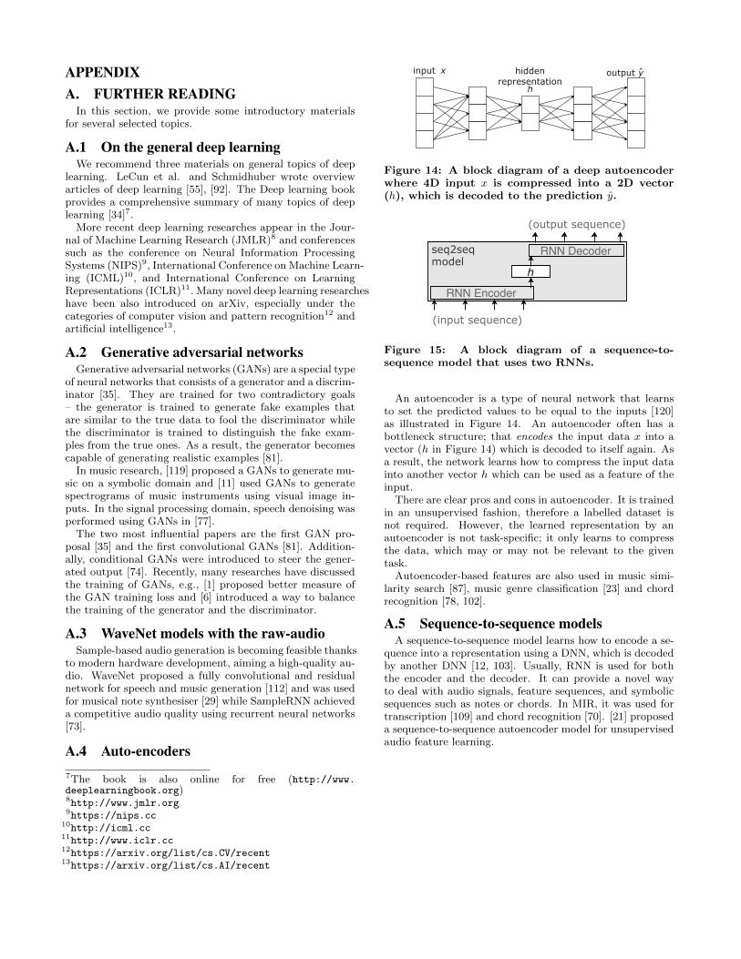
APPENDIXA. FURTHER READING

In this section, we provide some introductory materialsfor several selected topics.

A.1 On the general deep learningWe recommend three materials on general topics of deep

learning. LeCun et al. and Schmidhuber wrote overviewarticles of deep learning [55], [92]. The Deep learning bookprovides a comprehensive summary of many topics of deeplearning [34]7.

More recent deep learning researches appear in the Jour-nal of Machine Learning Research (JMLR)8 and conferencessuch as the conference on Neural Information ProcessingSystems (NIPS)9, International Conference on Machine Learn-ing (ICML)10, and International Conference on LearningRepresentations (ICLR)11. Many novel deep learning researcheshave been also introduced on arXiv, especially under thecategories of computer vision and pattern recognition12 andartificial intelligence13.

A.2 Generative adversarial networksGenerative adversarial networks (GANs) are a special type

of neural networks that consists of a generator and a discrim-inator [35]. They are trained for two contradictory goals– the generator is trained to generate fake examples thatare similar to the true data to fool the discriminator whilethe discriminator is trained to distinguish the fake exam-ples from the true ones. As a result, the generator becomescapable of generating realistic examples [81].

In music research, [119] proposed a GANs to generate mu-sic on a symbolic domain and [11] used GANs to generatespectrograms of music instruments using visual image in-puts. In the signal processing domain, speech denoising wasperformed using GANs in [77].

The two most influential papers are the first GAN pro-posal [35] and the first convolutional GANs [81]. Addition-ally, conditional GANs were introduced to steer the gener-ated output [74]. Recently, many researches have discussedthe training of GANs, e.g., [1] proposed better measure ofthe GAN training loss and [6] introduced a way to balancethe training of the generator and the discriminator.

A.3 WaveNet models with the raw-audioSample-based audio generation is becoming feasible thanks

to modern hardware development, aiming a high-quality au-dio. WaveNet proposed a fully convolutional and residualnetwork for speech and music generation [112] and was usedfor musical note synthesiser [29] while SampleRNN achieveda competitive audio quality using recurrent neural networks[73].

A.4 Auto-encoders7The book is also online for free (http://www.deeplearningbook.org)8http://www.jmlr.org9https://nips.cc

10http://icml.cc11http://www.iclr.cc12https://arxiv.org/list/cs.CV/recent13https://arxiv.org/list/cs.AI/recent

Figure 14: A block diagram of a deep autoencoderwhere 4D input x is compressed into a 2D vector(h), which is decoded to the prediction y.

Figure 15: A block diagram of a sequence-to-sequence model that uses two RNNs.

An autoencoder is a type of neural network that learnsto set the predicted values to be equal to the inputs [120]as illustrated in Figure 14. An autoencoder often has abottleneck structure; that encodes the input data x into avector (h in Figure 14) which is decoded to itself again. Asa result, the network learns how to compress the input datainto another vector h which can be used as a feature of theinput.

There are clear pros and cons in autoencoder. It is trainedin an unsupervised fashion, therefore a labelled dataset isnot required. However, the learned representation by anautoencoder is not task-specific; it only learns to compressthe data, which may or may not be relevant to the giventask.

Autoencoder-based features are also used in music simi-larity search [87], music genre classification [23] and chordrecognition [78, 102].

A.5 Sequence-to-sequence modelsA sequence-to-sequence model learns how to encode a se-

quence into a representation using a DNN, which is decodedby another DNN [12, 103]. Usually, RNN is used for boththe encoder and the decoder. It can provide a novel wayto deal with audio signals, feature sequences, and symbolicsequences such as notes or chords. In MIR, it was used fortranscription [109] and chord recognition [70]. [21] proposeda sequence-to-sequence autoencoder model for unsupervisedaudio feature learning.