JOURNAL OF RESEARCH of the National Bureau of Standards Vol. 86, No.5, September-October 1981

A Transient Hot Wire Thermal Conductivity Apparatus for Fluids*

Hans M. Rodert

National Bureau of Standards, Boulder, CO 80303

May 26, 1981

A new apparatus for measuring the thermal conductivity of fluids is described. This is an absolute method utilizing a transient hot wire. Measurements are made with a 12.7 p,m diameter platinum wire at real times of up to 1 second. The data acquisition system includes a minicomputer and a digital voltmeter. The experimental core of the system incorporates a compensating hot wire in a Wheatstone bridge circuit. The cell containing the core of the apparatus is designed to accommodate pressures from 0 to 70 MPa and temperatures from 70 to 320 K. Oxygel1 was measured over a wide range of physical states including the dilute gas, the moderately dense gas, the near critical region, the compressed liquid states, and the vapor ai temperatures below the critical temper· ature. Performance checks of the apparatus were conducted with nitrogen, helium and argon. Measurement of rare gases allows a direct comparison to the kinetic theory of gases through the viscosity. A second check looks at the variation of the measured thermal conductivity as a function of the applied power. The precision (2 a) of the new system is between 0.5 and 0.8 percent for wire temperature transients of 4 to 5 K, while the accuracy is estitnated at around 1.5 percent.

Key words: Helium; hot wire; nitrogen; pressure; temperature; thermal conductivity; transient.

1. Introduction 2. Method

Thermal conductivity values are necessary whenever a heat transfer problem is to be evaluated. In addition, ther­mal conductivity is a property of fundamental interest in developing the theory of fluids. Accurate measurements of thermal conductivity are of considerable difficulty. Methods and geometries abound each with its adherents and its in­herent drawbacks. The steady state hot wire experiment is one of the older, well established methods. The transient hot wire method, however, has come into its own only with recent advances in digital electronics. The evolution of the modern transient hot wire experiment can be traced from the early experiments of Pittman [1)1, Haarman [2], and Mani [3]. However, the major exposition of both theory and application of this method was accomplished by Kestin and his coworkers during the last decade [4-9] for the gas phase. Similar instruments have been used by Wakeham and his coworkers for both gas and liquid measurements [10, 11] and by de Castro and his coworkers for liquid meas­urements [12-13].

A hot wire system normally involves a vertical, cylindrical symmetry where the wire serves both as heating element and as thermometer. Almost without exception platinum is the wire of choice. The mathematical model that one at­tempts to approximate is that of an infinite line source of heat suspended vertically in an infinite medium. The method is labeled transient because the power is applied abruptly and the measurement is of short duration. The working equation is based on a specific solution of Fourier's law and can be found in standard texts (see for example reference [14], page 261).

_ _ q (4K) 1{t) - Tr ., - AT - 471'A En a2C t (1)

Where 1{t) is the temperature of the wire at time t;

·This work was carried out at the National Bureau of Standards under the sponsor· ship of the National Aeronautics and Space Administration (C-32369-C).

ffhermophysical Properties Division, National Engineering Laboratory. 1 Figures in brackets indicate literature references at the end of this paper.

457

Tr., is the reference temperature, the temperature of the cell;

q is the applied power; A is the thermal conductivity of the fluid, a function of

both temperature and density; K is the thermal diffusivity of the fluid, i.e., K =

AI e Cpo K is normally taken at the temperature T", and is nearly constant since the fluid properties do

not change drastically with a small increase in temperature;

a is the radius of the wire; and in C= 'Y where 'Y is Euler's constant.

The relation given by eq (1) implies a straight line for a plot of llT versus in(t). In practice systematic deviations occur at both short and long times. However, for each experimental measurement there exists a range of times over which eq (1) is valid, that is the relation between llT and fn(t) is linear. This range of validity is determined from 250 measured llT-t pairs by selecting a beginning time tl and an ending time t1 • The slope of the llT versus fn(t) relation is oblained over the valid range, i.e., between times t} and t2 , and using the applied power the thermal conductivity is calculated from eq (1). The temperature assigned to the measurement of A is given by

The density assigned to the measurement of A is taken from an equation of state using an experimentally measured pressure and the temperature assigned above. The equa­tions of state used for nitrogen and helium are given in subsequent sections. The experimentally determined teni­perature rise of the wire is llTw • A number of corrections ac­count for the departure of the real instrument from the ideal model:

(3)

These corrections oTt have been fully described elsewhere [5]; the most important at lower times is oT}, the effect of the finite heat capacity of the wire.

3. Apparatus

The various elements of the apparatus, the hot wires, the

long or primary hot wire is approximately 10 cm in length. Its resistance varies from about 20 {} at 76 K to 90 {} at 298 K. The short or compensating wire is approximately 5 cm in length and its resistance varies from 10 to 45 {}. To allow for thermal expansion over the range of operating tempera­tures the wires are mounted with a small weight attached at the bottom. The wires are mounted in the hard drawn (as received) state, because in the annealed state platinum has a rather low tensile strength [16].

3.2. High Pressure Cell and Wire Supports

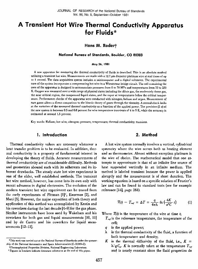
The cell has been designed to withstand pressures of up to 70 MPa. In addition; if the cell is to be isothermal, its thermal conductivity should be high. Accordingly, the cell is made from beryllium copper, a material which meets these contradictory requirements best. Cell sizing, cell Closure, and wire support are shown in figure 1. The cell is quite similar to those used in other experiments in this laboratory [17-20]. It is mounted with the closure facing down. Three solid steel pins serve as electrical leads. They pass through the high pressure closure (stainless steel) and are insulated

Ring

Refllx Yoke--+I--I~

Capilary

---1:f- RefkJx Tube

Platirun Resistance Thermometer Wei

high pressure cell and wire supports, the Wheatstone High Pres~e Cel--\!--t-t-t-t+-:,\,J

bridge, the cryostat, the measuring and control circuitry, the sample handling system, and the minicomputer are de- Cel Radiation Shield

scribed here and in figures 1-6.

3.1. The Hot Wires

Platinum wire is the normal choice because the resist­ance-temperature relation of platinum is well known [15]. In the resistance thermometer grade of the wire the smallest sizes available commercially are 7 Ilm, 12.7 Ilm, and 25.4 Ilm in diameter. The smallest of these was considered to be too fragile for the present application, the largest would not provide a sufficiently large resistance for the cell size under consideration. Therefore, the 12.7 Ilm diameter wire was chosen for both primary and compensating hot wire. The

458

Copper 0 Ring

Potymide FemAe

Cel CIo~e --++--+ ...... , "

EIectricaJ Lead Through

FIGURE 1. The high pressure cell and wire support unit.

Covers

from it using polymide ferrules [21]. The capillary which ad­mits the sample is soldered into the top of the cell. Much of the interior of the cell is filled by the wire support unit which is made from copper and includes a centerpiece, two covers, a top and a bottom cap. The wire support unit is mounted on the high pressure closure. When assembled the wire support unit provides two cylindrical wells 9 mm in diameter and 11 cm long to accomodate the hot wires. Mounted in the top cap with friction fit are two 5 mm sec­tions of a small coaxial cable. The hot wires are soft soldered to the center leads of these coaxial sections. To the bottom of the long hot wire is soldered a short section of teflon covered wire which terminates in a 4-80 brass nut, the weight. The teflon covered section provides isulation be­tween bottom cap and the extension of the long hot wire as well as centering for it. The long hot wire section is con­nected to one of the steel pins by a small loop of 12.7 p.m copper wire. The short hot wire is soft soldered to the other coaxial section in the top cap. To its bottom end a short length of copper wire centered in a second 4-80 brass nut is soldered. The leads on the short hot wire side are completed by a loop of 12.7 p.m copper wire which connects to a 5 em length of coaxial cable. This section of coax is friction fit into the bottom cap and is sufficiently rigid to stand alone. A second loop of copper connects this coax to the second steel pin. Long and short hot wire sections are connected together above the top cap with the center tap soldered in the middle of this connection. The center tap is a 11 cm long section of the coax which at the bottom end is con­nected to the third steel pin.

Liquid oxygen safety is one of the additional design con­siderations for the cell since the interior of the cell will be exposed to very high pressure 70 MPa (10,000 psi) liquid. The materials directly exposed to liquid oxygen have been limited to beryllium copper, copper, stainless steel, silver, teflon, and a polyimide (kapton) all of which have been found to be Uoxygen compatible" [22]. Cleaning procedures for cell, wire supports, capillary and sample handling system were extensive [23].

3.3. The Wheatstone Bridge

Precision measurements of resistance can be made by us­ing a four lead technique or by using a Wheatstone bridge. In the present apparatus we follow the general development of the hot wire instrument pioneered by Haarman [2], de Groot, et al. [4], Assael, et al. [10] and de Castro, et al. [12] and use a Wheatstone bridge to measure resistances. End effect compensation is provided by placing the long hot wire in one working arm of the bridge and a shorter, com­pensating wire on the other. In contrast to other instru­ments where values of time are measured in the present instrument the voltage developed across the bridge is

measured directly as a function of time with a fast response digital voltmeter (DVM). The DVM is controlled by a mini­computer which also handles the switching of the power and the logging of the data. The automation of the voltage measurement follows the work of Mani [3] who used a similar arrangement with a transient hot wire cell to meas­ure resistance by the four lead technique rather than using a bridge.

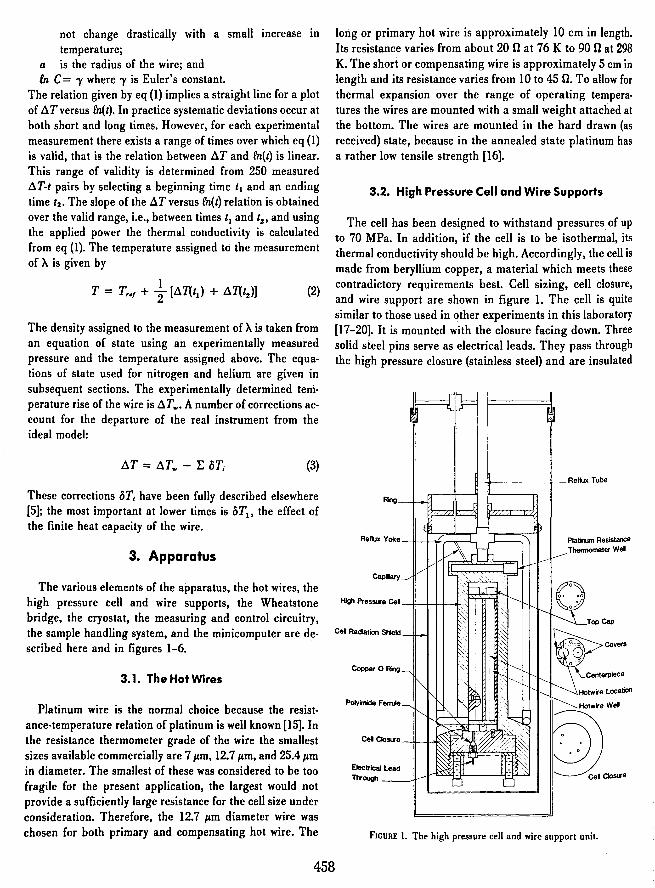
Figure 2 shows the Wheatstone bridge circuit. Each arm of the bridge is designed to be 100 n, two arms Rl and R2 are standard resistors. The resistance in each of the other arms R3 and R. is a composite of the hot wire, the leads into the cryostat and an adjustable ballast resistor. The leads are roughly 6 n at room temperature and 2 n when the cell is at 76 K. The ballast resistors allow each working arm to be ad­justed to a value of 100 n.

The measurement of thermal conductivity for a single point is accomplished in two phases. In the first phase the bridge is balanced as close to null as is practical. To start with, switch 1 is turned from dummy to the bridge while switch 2 is open. With a very small applied voltage, 0.1 Volts normally, and the cell essentially at constant tempera­ture, the voltages are read on channels 0 through 7. The lead, hot wire, and ballast resistances are calculated from the ratios of the appropriate channel volt gage to the voltage across the standard lOOn resistor on channel zero. The ballasts are adjusted until each leg is approximately 100 n. Finally, with switch 2 closed, the bridge null is checked on channel 6. The second phase incorporates the actual ther­mal conductivity measurement. The power supply is set to the applied power desired, switch 2 is closed, and switch 1 is switched from dummy to bridge. The voltage developed across the bridge as a function of time is read on channel 6 and stored. The basic data is a set of 250 readings taken at 3 ms intervals. Finally the voltage on channel 0 is read to de­termine the exact applied power, and the power is switched back to the dummy resistor.

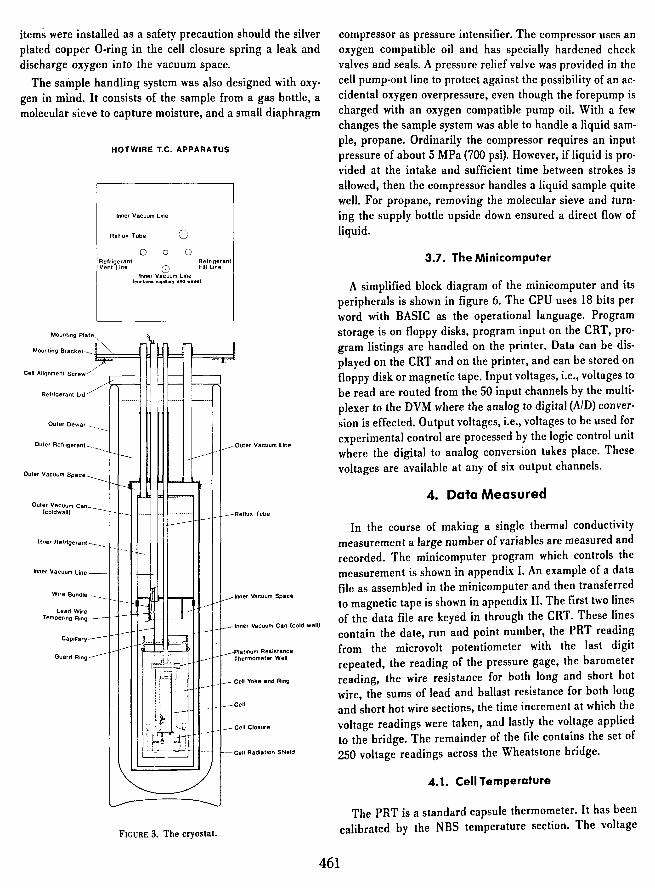
3.4. The Cryostat

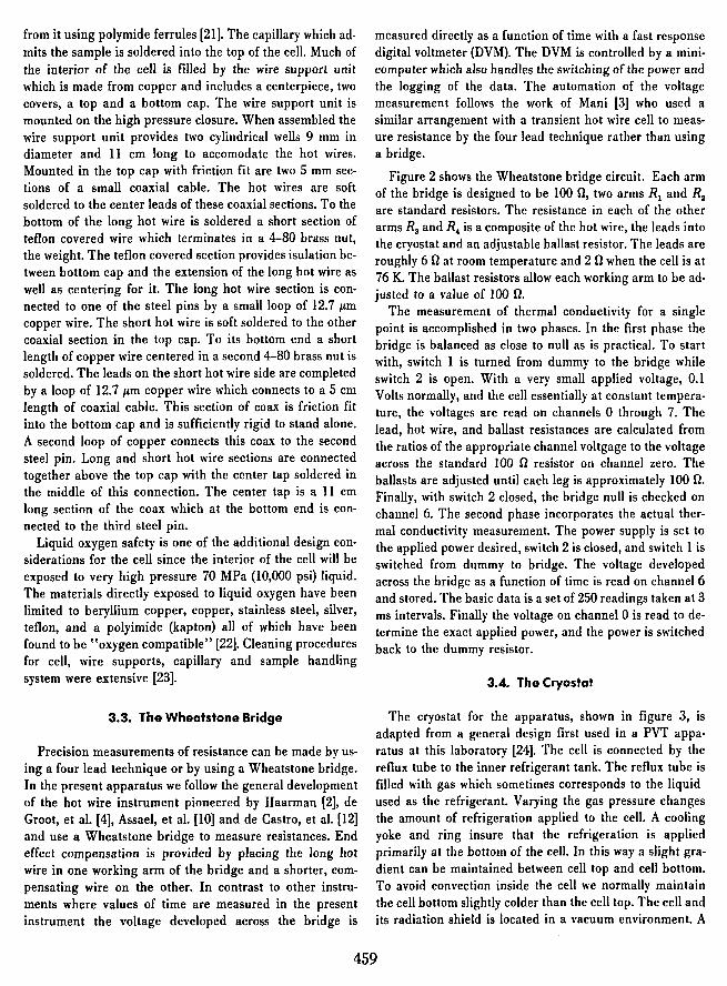
The cryostat for the apparatus, shown in figure 3, is adapted from a general design first used in a PVT appa­ratus at this laboratory [24]. The cell is connected by the reflux tube to the inner refrigerant tank. The reflux tube is filled with gas which sometimes corresponds to the liquid used as the refrigerant. Varying the gas pressure changes the amount of refrigeration applied to the cell. A cooling yoke and ring insure that the refrigeration is applied primarily at the bottom of the cell. In this way a slight gra­dient can be maintained between cell top and cell bottom. To avoid convection inside the cell we normally maintain the cell bottom slightly colder than the cell top. The cell and its radiation shield is located in a vacuum environment. A

459

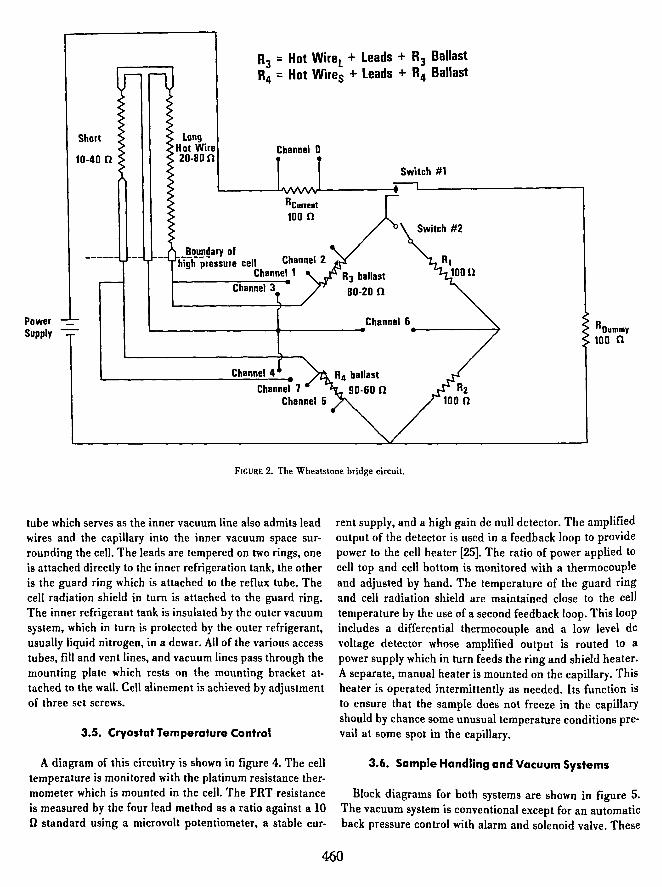
RJ = Hot WireL + Leads + R3 Ballast R4 :: Hot Wires + Leads + R4 Ballast

Short

10-40 n

Long Hot Wire 20-80 n

Channel 0

Boundary of highpressure cell Channel 2

Channel 1 Channel J

Channel 6 Power Supply

~ ________________ -+ __________ -4 .-----------~ Roummy 100 n

Channel 4

FIGURE 2. The Wheatstone bridge circuit.

tube which serves as the inner vacuum line also admits lead wires and the capillary into the inner vacuum space sur­rounding the cell. The leads are tempered on two rings, one is attached directly to the inner refrigeration tank, the other is the guard ring which is attached to the reflux tube. The cell radiation shield in turn is attached to the guard ring. The inner refrigerant tank is insulated by the outer vacuum system, which in turn is protected by the outer refrigerant, usually liquid nitrogen, in a dewar. All of the various access tubes, fill and vent lines, and vacuum lines pass through the mounting plate which rests on the mounting bracket at­tached to the wall. Cell alinement is achieved by adjustment of three set screws.

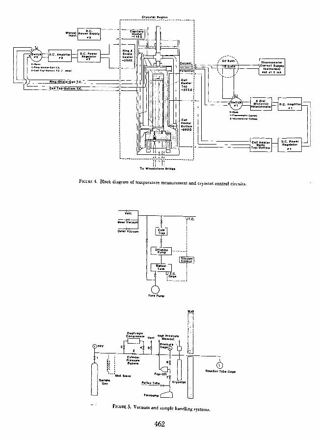
3.5. Cryostat Temperature Control

A diagram of this circuitry is shown in figure 4. The cell temperature is monitored with the platinum resistance ther­mometer which is mounted in the cell. The PRT resistance is measured by the four lead method as a ratio against a 10 o standard using a microvolt potentiometer, a stable cur-

rent supply, and a high gain de null detector. The amplified output of the detector is used in a feedback loop to provide power to the cell heater [25]. The ratio of power applied to cell top and cell bottom is monitored with a thermocouple and adjusted by hand. The temperature of the guard ring and cell radiation shield are maintained close to the cell temperature by the use of a second feedback loop. This loop includes a differential thermocouple and a low level dc voltage detector whose amplified output is routed to a power supply which in turn feeds the ring and shield heater. A separate, manual heater is mounted on the capillary. This heater is operated intermittently as needed. Its function is to ensure that the sample does not freeze in the capillary should by chance some unusual temperature conditions pre­vail at some spot in the capillary.

3.6. Sample Handling and Vacuum Systems

Block diagrams for both systems are shown in figure 5. The vacuum system is conventional except for an automatic back pressure control with alarm and solenoid valve. These

460

items were installed as a safety precaution should the silver plated copper O-ring in the cell closure spring a leak and discharge oxygen into the vacuum space.

The sample handling system was also designed with oxy­gen in mind. It consists of the sample from a gas bottle, a molecular sieve to capture moisture, and a small diaphragm

HOTWIRE T.e. APPARATUS

Inner Vacuum line

Reflu. Tube 0 000

Refrigerant Refrigerant Vent Line 8 Fill Line

Inner Vacuum Line (eonlainscapiRary and wir •• '

Mounting Plate

Mounting Bracket ~~=~

Cell Alignment Screw

Refrigerant Lid

Outer Dewar

Outer Refrigerant ______

Outer Vacuum Space

Outer Vacuum Can I (coldwall) ~-

I

Inner Refrigerant ______

Inner Vacuum Line ---t---t--++--l-

Wire Bundle ___

Lead Wire Tempering Ring _.J-.-+----tT<lI I

Capillary

Guard Ring-------

Outer Vacuum line

Reftu. Tube

Inner Vacuum Space

Inner Vacuum Can (cold wall)

Platinum Resistance Thermometer Well

Cell Yoke and Ring

_Cell

Cen Closure

--- - -Cell Radiation Shield

FIGURE 3. The cryostat.

compressor as pressure intensifier. The compressor uses an oxygen compatible oil and has specially hardened check valves and seals. A pressure relief valve was provided in the cell pump-out line to protect against the possibility of an ac­cidental oxygen overpressure, even though the forepump is charged with an oxygen compatible pump oil. With a few changes the sample system was able to handle a liquid sam­ple, propane. Ordinarily the compressor requires an input pressure of about 5 MPa (700 psi). However, if liquid is pro­vided at the intake and sufficient time between strokes is allowed, then the compressor handles a liquid sample quite well. For propane, removing the molecular sieve and turn­ing the supply bottle upside down ensured a direct flow of liquid.

3.7. The Minicomputer

A simplified block diagram of the minicomputer and its peripherals is shown in figure 6. The CPU uses 18 bits per word with BASIC as the operational language. Program storage is on floppy disks, program input on the CRT, pro­gram listings are handled on the printer. Data can be dis­played on the CRT and on the printer, and can be stored on floppy disk or magnetic tape. Input voltages, i.e., voltages to be read are routed from the 50 input channels by the multi­plexer to the DVM where the analog to digital (AiD) conver­sion is effected. Output voltages, i.e., voltages to be used for experimental control are processed by the logic control unit where the digital to analog conversion takes place. These voltages are available at any of six output channels.

4. Data Measured

In the course of making a single thermal conductivity measurement a large number of variables are measured and recorded. The minicomputer program which controls the measurement is shown in appendix I. An example of a data file as assembled in the minicomputer and then transferred to magnetic tape is shown in appendix II. The first two lines of the data file are keyed in through the CRT. These lines contain the date, run and point number, the PRT reading from the microvolt potentiometer with the last digit repeated, the reading of the pressure gage, the barometer reading, the wire resistance for both long and short hot wire, the sums of lead and ballast resistance for both long and short hot wire sections, the time increment at which the voltage readings were taken, and lastly the voltage applied to the bridge. The remainder of the file contains the set of 250 voltage readings across the Wheatstone bridge.

4.1. Cell Temperature

The PRT is a standard capsule thermometer. It has been calibrated by the NBS temperature section. The voltage

461

IIln IShl.ld-C." T.C.

[L[----~C~.I~IT=Op--=Bo="o=m~T~.C-. ----------

1 I

: I I

: l----------------rrnr-------------To Wh .... ton. Brldg.

"'---..... ,, I 011 Bath \

I \

.t

FIGURE 4. Block diagram of temperature measurement and cryostat control circuits.

Ol<lphragm Compressor

Wan

FIGURE 5. Vacuum and sample handling systems.

462

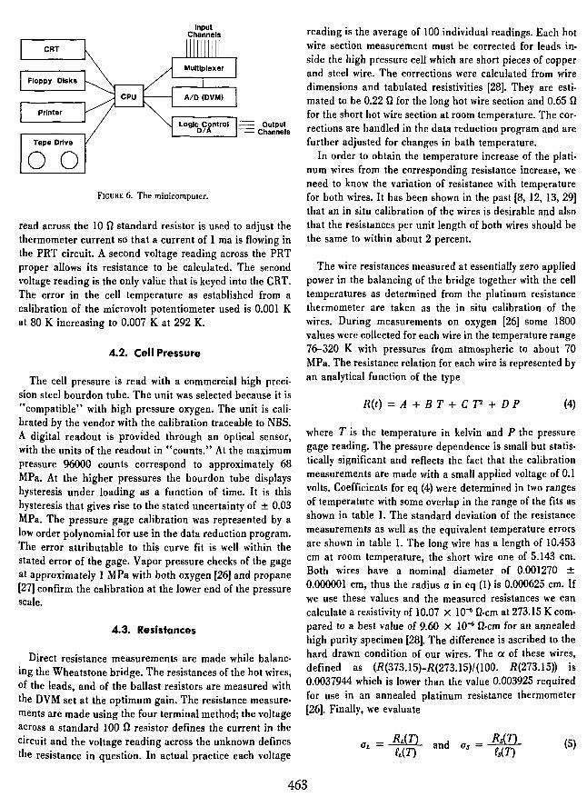
00 FIGURE 6. The minicomputer.

Output Channels

read across the 10 {} standard resistor is used to adjust the thermometer current so that a current of 1 rna is flowing in the PRT circuit. A second voltage reading across the PRT proper allows its resistance to be calculated. The second voltage reading is the only value that is keyed into the CRT. The error in the cell temperature as established from a calibration of the microvolt potentiometer used is 0.001 K at 80 K increasing to 0.007 K at 292 K.

4.2. Cell Pressure

The cell pressure is read with a commercial high preci­sion steel bourdon tube. The unit was selected because it is Ucompatible" with high pressure oxygen. The unit is cali­brated by the vendor with the calibration traceable to NBS. A digital readout is provided through an optical sensor, with the units of the readout in Ucounts." At the maximum pressure 96000 counts correspond to approximately 68 MPa. At the higher pressures the bourdon tube displays hysteresis under loading as a function of time. It is this hysteresis that gives rise to the stated uncertainty of ± 0.03 MPa. The pressure gage calibration was represented by a low order polynomial for use in the data reduction program. The error attributable to this curve fit is well within the stated error of the gage. Vapor pressure checks of the gage at approximately 1 MPa with both oxygen [26] and propane [27] confirm the calibration at the lower end of the pressure scale.

4.3. Resistances

Direct resistance measurements are made while balanc­ing the Wheatstone bridge. The resistances of the hot wires, of the leads, and of the ballast resistors are measured with the DVM set at the optimum gain. The resistance measure­ments are made using the four terminal method; the voltage across a standard 100 {} resistor defines the current in the circuit and the voltage reading across the unknown defines the resistance in question. In actual practice each voltage

reading is the average of 100 individual readings. Each hot wire section measurement must be corrected for leads in­side the high pressure cell which are short pieces of copper and steel wire. The corrections were calculated from wire dimensions and tabulated resistivities [28]. They are esti­mated to be 0.22 {} for the long hot wire section and 0.65 {} for the short hot wire section at room temperature. The cor­rections are handled in the data reduction program and are further adjusted for changes in bath temperature.

In order to obtain the temperature increase of the plati­num wires from the corresponding resistance increase, we need to know the variation of resistance with temperature for both wires. It has been shown in the past [8, 12, 13,29] that an in situ calibration of the wires is desirable and also that the resistances per unit length of both wires should be the same to within about 2 percent.

The wire resistances measured at essentially zero applied power in the balancing of the bridge together with the cell temperatures as determined from the platinum resistance thermometer are taken as the in situ calibration of the wires. During measurements on oxygen [26] some 1800 values were collected for each wire in the temperature range 76-320 K with pressures from atmospheric to about 70 MPa. The resistance relation for each wire is represented by an analytical function of the type

R(t) = A + B T + C 'J'2 + D P (4)

where T is the temperature in kelvin and P the pressure gage reading. The pressure dependence is small but statis­tically significant and reflects the fact that the calibration measurements are made with a small applied voltage of 0.1 volts. Coefficients for eq (4) were determined in two ranges of temperature with some overlap in the range of the fits as shown in table 1. The standard deviation of the resistance measurements as well as the equivalent temperature errors are shown in table 1. The long wire has a length of 10.453 cm at room temperature, the short wire one of 5.143 cm. Both wires have a nominal diameter of 0.001270 ± 0.000001 cm, thus the radius a in eq (1) is 0.000625 cm. If we use these values and the measured resistances we can calculate a resistivity of 10.07 X 10-6 {}-cm at 273.15 K com­pared to a best value of 9.60 X 10-6 O-cm for an annealed high purity specimen [28]. The difference is ascribed to the hard drawn condition of our wires. The a of these wires, defined as (R(373.l5)-R(273.l5)/(100. R(273.15» is 0.0037944 which is lower than the value 0.003925 required for use in an annealed platinum resistance thermometer [26]. Finally, we evaluate

463

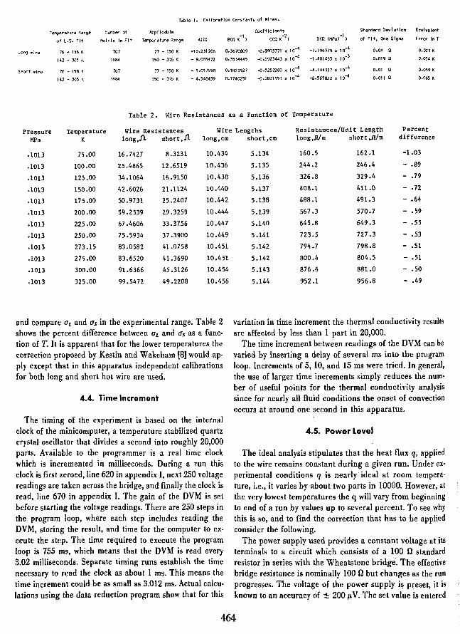
Table I. Calibration Constants of Wires.

Number of Coeff I e I ents St and ard Dev I at I on Equivalent Temperature Range Applicable

B(O K-1 I -2 -1

of L.S. Fit Points In Fit Temperature Range A({ll C(O K I D(O (MPal I of Fit, One Sigma Error In T

Long olre 76 - 158 K 707 77 - 150 K -10.231206 0.3670809 ~.9903371 )( 10-4 -7.796325)( 10-4 0.01 0 0.023 K

142 - 305 K 1684 150 - 315 K - 9.0654n 0.3534445 ~.5923443 )( 10-4 -1.401463 )( 10-3 0.019 0 0.054 K

Short olre 76 - 158 K 707 77 - 150 K - 5.057558 0.1823527 ~.525n80 x 10-4 -4.144377 )( 10-4 0.01 0 0.059 K

142 - 305 K 1684 150 - 315 K - 4.346459 0.1740251 ~.2831553 x 10-4 -<;.565822 )( 10-4 0.011 0 0.065 K

Table 2. Wire Resistances as a Function of Temperature

Pressure Temperature Wire Resistances Wire Lengths Resistances/Unit Length Percent

MPa K long,l1 short,lt long,cm

.1013 75.00 16.7427 8.3231 10.434

.1013 100.00 25.4865 12.6519 10.436

.1013 125.00 34.1064 16.9150 10.438

.1013 150.00 42.6026 21.1124 10.440

.1013 175.00 50.9731 25.2407 10.442

.1013 200.00 59.2539 29.3259 10.444

.1013 225.00 67.4606 33.3756 10.447

.1013 250.00 75.5934 37.3900 10.449

.1013 273.15 83.0582 41.0758 10.451

.1013 275.00 83.6520 41.3690 10.451

.1013 300.00 91.6j66 45.3126 10.454

.1013 325.00 99.5472 49.2208 10.456

and compare (h and (Js in the experimental range. Table 2 shows the percent difference between (JL and (Js as a func­tion of T. It is apparent that for the lower temperatures the correction proposed by Kestin and Wakeham [8] would ap­ply except that in this apparatus independent calibrations for both long and short hot wire are used.

4.4. Time Increment

The timing of the experiment is based on the internal clock of the minicomputer, a temperature stabilized quartz crystal oscillator that divides a second into roughly 20,000 parts. Available to the programmer is a real time clock which is incremented in milliseconds. During a run this clock is first zeroed, line 620 in appendix I, next 250 voltage readings are taken across the bridge, and finally the clock is read, line 670 in appendix I. The gain of the DVM is set before starting the voltage readings. There are 250 steps in the program loop, where each step includes reading the DVM, storing the result, and time for the computer to ex­ecute the step. The time required to execute the program loop is 755 ms, which means that the DVM is read every 3.02 milliseconds. Separate timing runs establish the time necessary to read the clock as about 1 ms. This means the time increment could be as small as 3.012 ms. Actual calcu­lations using the data reduction program show that for this

short,cm long,ll/m short,J1/m difference

5.134 160.5 162.1 -1.03

5.135 244.2 246.4 - .89

5.136 326.8 329.4 - .79

5.137 408.1 411.0 - .72

5.138 488.1 491.3 - .64

5.139 567.3 570.7 - .59

5.140 645.8 649.3 - .55

5.141 723.5 727.3 - .53

5.142 794.7 798.8 - .51

5.142 800.4 804.5 - .51

5.143 876.6 881.0 - .50

5.144 952.1 956.8 - .49

variation in time increment the thermal conductivity results are affected by less than 1 part in 20,000.

The time increment between readings of the DVM can be varied by inserting a delay of several ms into the program loop. Increments of 5, 10, and 15 ms were tried. In general, the use of larger time increments simply reduces the num­ber of useful points for the thermal conductivity analysis since for nearly all fluid conditions the onset of convection occurs at around one second in this apparatus.

4.5. Power Level

The ideal analysis stipulates that th~ heat flux q, applied to the wire remains constant during a given run. Under ex­perimental conditions q is nearly' ideal at room tempera­ture, i.e., it varies by about two parts in 10000. However, at the very lowest temperatures the q will vary from beginning to end of a run by values up to several percent. To see why this is so, and to find the correction that has to he applied consider the following.

The power supply used provides a constant voltage at its terminals to a circuit which consists of a 100 n standard resistor in series with the Wheatstone bridge. The effective bridge resistance is nominally 100 n but changes as the run progresses. The voltage of the power supply i~ preset, it is known to an accuracy of ± 200 p. V. The set value is entered

464

through the key board, just prior to switching the power to the bridge. After the run is completed, but before the power is switched back to the dummy resistor; the voltage across the standard resistor, channel 0 in figure 2, is read. The dif­ference between this voltage and the preset one is the voltage applied to the bridge a short time after completion of the run. The difference is one of the items placed on magnetic tape, and it is used in the data reduction program to calculate the power applied to the bridge. The instan­taneous heat flux is determined from the equation.

(6)

where V(t) is the voltage applied to the bridge, and R3 and R4 are defined in figure 2. The voltage V(t), both hot wire legs of the bridge R3 and R4 , and the hot wire resistances themselves change as a function of time. At room tempera­ture the drop in the current is almost exactly offset by the rise in the hot wire resistances. At low temperatures the fractional change in the hot wire resistances predominates. As an extreme example consider a run in liquid propane at say 110 K. For a 3 K rise in wire temperature the long hot wire rises by 1 n from an initial value of 30 0, or 3.3 per­cent. This rise is only partially offset by the 0.7 percent drop

> E

Q) ry co

o > Q) ry D

++

2 +

in the hot wire current leaving a net rise in q of 2.6 percent from t = 0 to t = 755 ms. The range of valid times for a run is generally t} = 150 ms, t2 = 755 ms. Over this range of times the variation in q is less than the extreme case because a large part, 70 percent or so, of the resistance change of the hot wires occurs during the times not valid for the experiment. Nevertheless, the remaining variation in q is significant and we apply a correction to account for it. We select. a time in the middle of the valid time interval ta = (t} + t2)/2 and correct the experimental ilT's by the ratio of the instantaneous q to the q at the median time

ilT(t)co •• = ilT(t).aw • q(tj)1 q(ta) .... (7)

V(t) varies by about one part in 1000 over a run, and some calculation verified that V(t) varies as the in(t), and further that the value measured was actually achieved at the req­uisite time after the end of the run.

4.6. Bridge Voltages

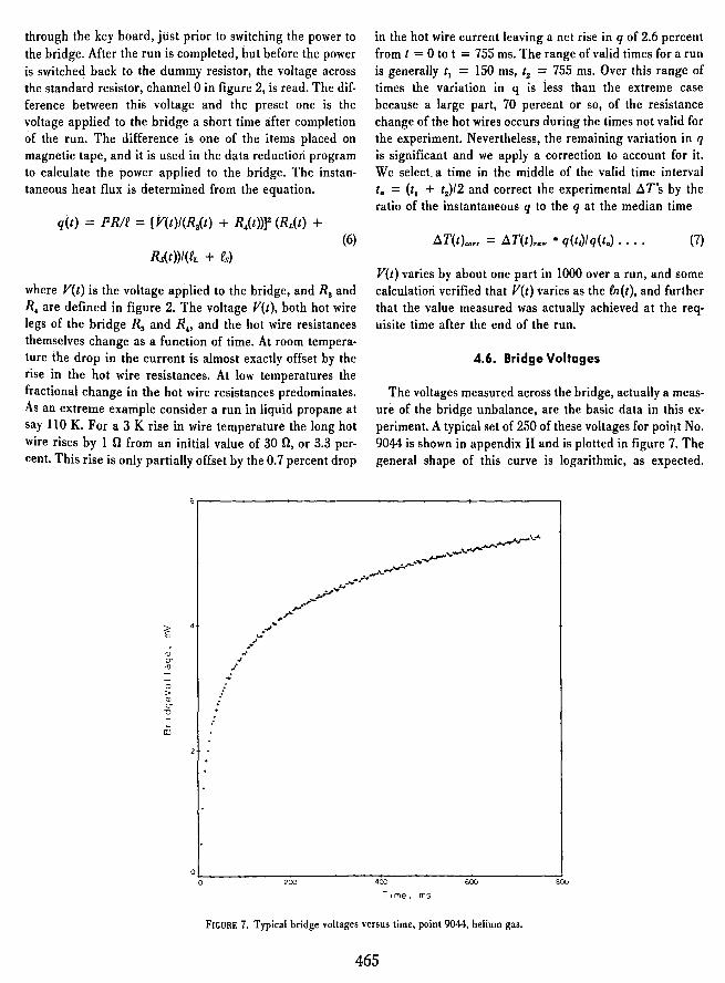
The voltages measured across the bridge, actually a meas­ure of the bridge unbalance, are the basic data in this ex­periment. A typical set of 250 of these voltages for point No. 9044 is shown in appendix II and is plotted in figure 7. The general shape of this curve is logarithmic, as expected.

O~O-------------------~2~OO~------------------4~OO~--------~~-----------~800

Time. ms

FIGURE 7. Typical bridge voltages versus time, point 9044, helium gas.

465

Noise levels in these readings are evident. Considerable ef­fort went into reducing the noise level, and also into tracing the source. The DVM, when shorted, exhibits an error band of ± 6 p.V. When a 100 0 resistor is placed across the DVM, no applied power yet, the band increases to ± 17 p. V. With the experimental system connected to the DVM the error band becomes ± 28 p. V which is roughly equivalent to ± .026 K in the llT. Only a small part, some 20 or 30 per­cent, is due to AC pickup. Use of integrating or averaging DVM's will reduce the noise level at the expense, however, of a smaller number of measurements.

5. Data Reduction

A listing of the data reduction program used for helium is given in appendix III. Experimental values are read from the magnetic tape. Initial calculations and corrections in­chide corrections for the bias of the DVM, corrections for the leads inside the high pressure cell, and an estimation of the instantaneous voltage applied to the bridge. The AT.., values are calculated from the voltages applied to the bridge, the offset or measured voltages across the bridge and the two hot wire calibrations. The bridge equation is solved repeatedly until the increases in the hot wire resistances together with the voltage applied to the bridge

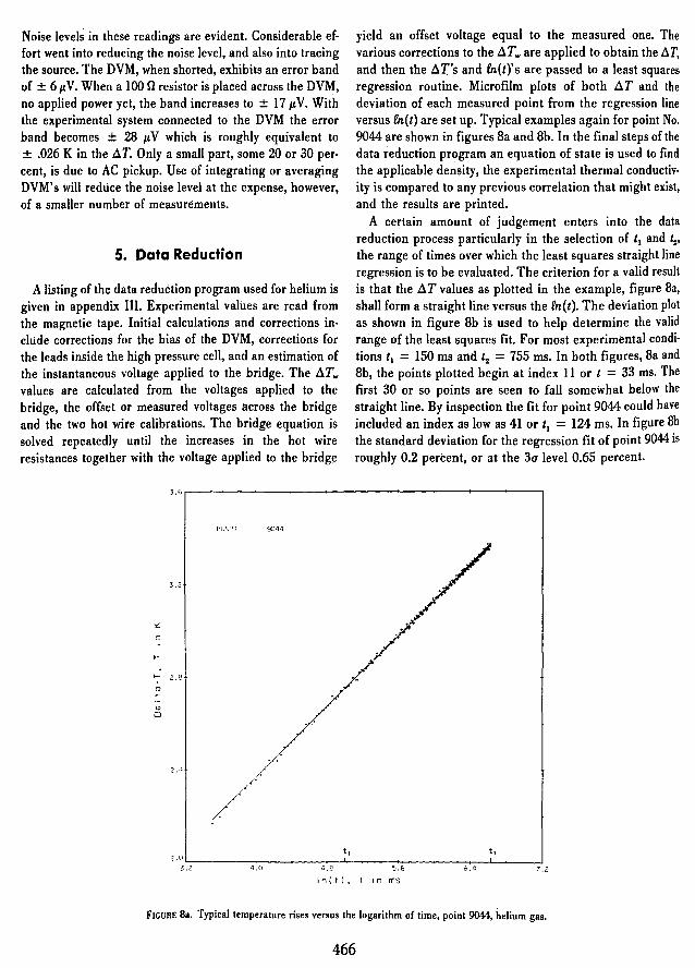
yield an offset voltage equal to the measured one. The various corrections to the AT.., are applied to obtain the AT, and then the Ar's and In{t)'s are passed to a least squares regression routine. Microfilm plots of both llT and the deviation of each measured point from the regression line versus In{t) are set up. Typical examples again for point No. 9044 are shown in figures 8a and 8b. In the final steps of the data reduction program an equation of state is used to find the applicable density, the experimental thermal conductiv­ity is compared to any previous correlation that might exist, and the results are printed.

A certain amount of judgement enters into the data reduction process particularly in the selection of tl and t: j

the range of times over which the least squares straight line regression is to be evaluated. The criterion for a valid result is that the AT values as plotted in the example, figure 8a, shall form a straight line versus the In{t). The deviation plot as shown in figure 8b is used to help determine the valid range of the least squares fit. For most experimental condi­tions tl = 150 ms and t2 = 755 ms. In both figures, 8a and 8b, the points plotted begin at index 11 or t = 33 ms. The first 30 or so points are seen to fall somewhat below the straight line. By inspection the fit for point 9044 could have included an index as low as 41 or tl = 124 ms. In figure 8b the standard deviation for the regression fit of point 9044 is roughly 0.2 percent, or at the 3u level 0.65 percent.

3.&r---------------------------~------------------,

PUNPT 9044

3.2

'Y

C

~

~ 2.8

:u -(I)

0

2.4

2·~~.2---------4.-0--------4~.g~~-----5-.&---------&.~4~------~7.2 In( I). I In ms

FIGURE 8a. Typical temperature rises versus the logarithm of time, point 9044, helium gas.

466

.8r---------+---------~--______ ~--------~----____ ~

RUNPT ,,044

• 4 ' . .... +. + STAT

C (lJ

u ... (lJ

Q

0.0

LL

(J) ....J

." .' . ... '. '.': ) ... "\. ... :....... +.+: +. + •• :./ •••••

.... + •• 1> .....

• .', "'i' ··.f ... ' '\

• " : t ,:' ... +, ~ )

.+.1' .++

E a

... + •• + ... +. • ,.... - STAT ... - - .4

C a )

I ~

co

> (lJ

0 - .8

t\ t2

. 1 .~ L. 2----~---4 ....... 0---------4 ..... -8 -L-----5-+.-" -------"--..-4 ---l------...J

7. 2

I n( t). tin ms

FIGURE Bb. Typical deviations of experimental temperature rises from the calculated straight line versus the logarithm of time, point 9044, helium gas.

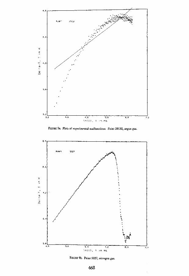
By implication, it is equally important to recognize and interpret nonstandard results obtained, so that invalid results can be identified and rejected. A description of several of the more interesting malfunctions follows. In figure 9a we see that the ilT values are nearly constant toward the end of the run. This state of affairs depending on the state of the fluid sample is interpreted as (a) the ap­paratus is operating in the steady state mode, or (b) as the onset of convection in the run.

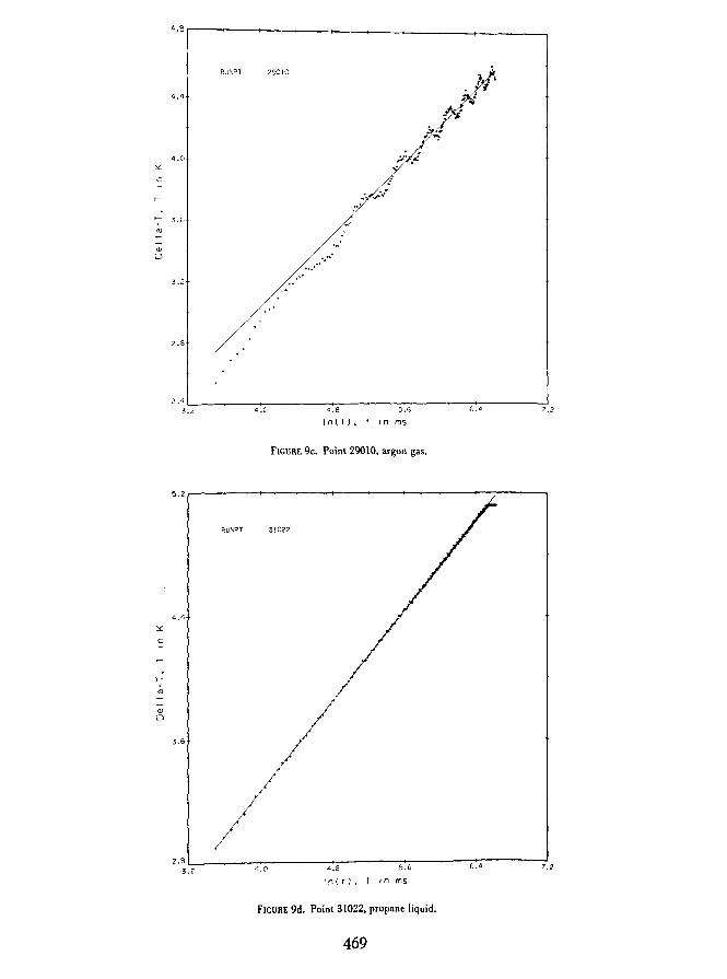
If a similar run at higher fluid densities is taken to much longer experimental times the plot is as shown in figure 9b. Here the effect of convection is clearly seen as a rapid cool­ing of the hot wires after the maximum ilT is passed. In principle we could get a valid result for the transient hot wire by selecting t} = 690 ms and t2 = 1353 ms. However, the number of ilT values useful for the straight line regres­sion has now dropped to 50. In practice it turns out that the applied power level, as seen in the resulting ilT's of 10 to 12 K, was simply too large to be useful. The plot of figure 9c shows the effect of gas circulation within the cell. The precise cause is not known. Convection combined with ther­mal oscillations when the capillary cools are suspected reasons. From the plot it is clear that the wires experience a non-uniform temperature field and are subject to abrupt segments of convection cooling. Measurements with a plot of this type are rejected.

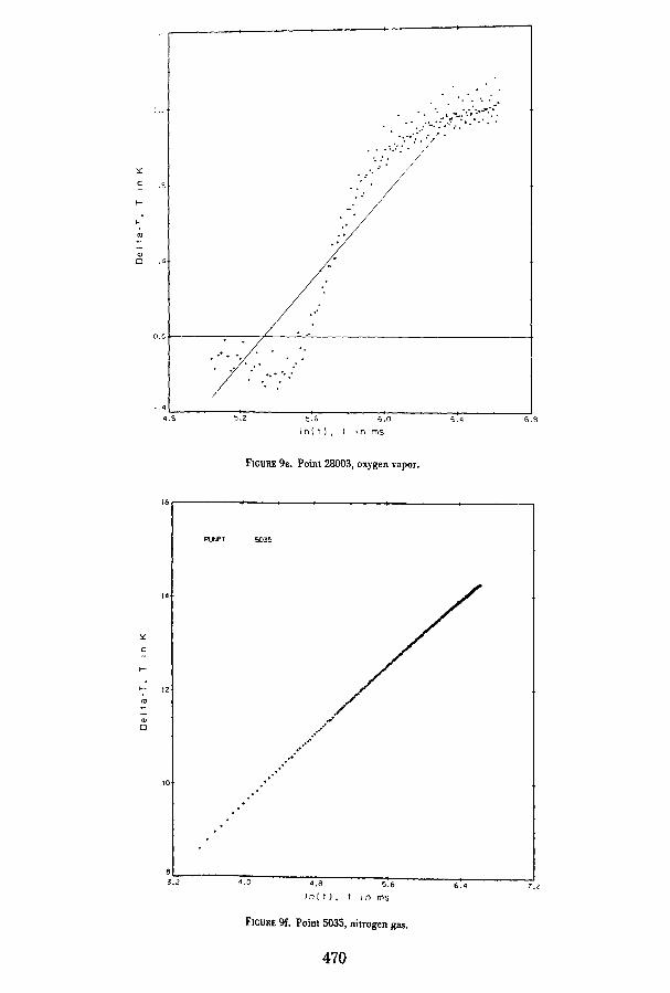
In figure 9d the DVM saturated toward the end of the run. By excluding the points for which the voltage readings are constant, and provided there are sufficient measure­ments to extract a straight line fit, a measurement of this type can be used. At the very lowest pressures (densities) in the vapor phase at temperatures much below the critical temperature some plots look like the one shown in figure ge. The physical interpretation of this run is that we see a Knudsen effect at short times and an outer boundary effect at the longer times. No valid range for the hot wire instru­ment exists and these results are rejected. In the region near the critical point the onset of convection occurs much more rapidly. Measurements in this fluid region have to be made at lower power levels and at shorter times. For the measurements on oxygen experimental times of tl == 33 ms and t2 == 500 ms were found to be appropriate.

A second criterion which is used in accepting or rejecting experimental measurements is by considering the change in the measured thermal conductivity as the applied power, q, is varied. Examples are given in the sections on nitrogen and helium. In a general way this criterion suggests that measurements in which the final ilT's are larger than about 5 K are suspect. This includes most of the critical region where the results have to be evaluated quite carefully, almost on an individual point by point basis.

467

4.8~· _____ -------------------+-;'7"---, RUNPT 29132

4.4

~ +.+

C

+++ l-

++

I- 4.0

~ .. ,

.' Ql 0

.'

3.6

3.2L-________ ~----------~----------~~--------~~--------~ 3.2 4.0 4.8 '5.6 6.4 7.2

In\ I). I In ms

F,CURE 9a. Plots of experimental malfunctions. Point 29132, argon gas.

e.er---------~--________ ~----______ ~----______ _+----------~

R\H'T 5027

8.0

~

c:

l-

I- 7.2

~

Ql [)

&.4

5·~~.8~--------~5+.6~--------~6~.-4-----------7~.2-----------8+.0----------~~." In( I). t In ms

F,CURE 9b. Point 5027, nitrogen gas.

468

4'~r---~----~------~~--____ ~ ________ -+ ________ _

RUNPT 29010

'l.'l

. . "1.0

~ ~ .. ~

c f

I- -' ".;. .. /

I- 3.G .. ' ro

.~

OJ 0 .... ..

••• +

3.2 .. '

2.8

2.4L-______ ----~----______ _+----------~------+-----+_----____ ~ 3.2 4.0 4.8 5.6 G.4 7.2

In( t). I In ms

FIGURE 9c. Point 29010, argon gas.

5.2.-----------~----------~--------'-~--------~--~------~

RUNPT 31022

4.4

~

C

l-

I-

:0 /

OJ , 0 /

3.G

/ 2.8L-______ --~----------~--------------------~~--------..j

3.2 4.0 4.8 5.6 0. 4 7.2

In( t). I In ms

FIGURE 9d. Point 31022, propane liquid.

469

c "

I-

.'

Q)

o .4

.. ' o.o~------------~L---~~-----------------------------------t

.+. + •

.' • + .+ +.+ +*.+

'. /

.. 4L-________ ~ ________ ~----______ ~----____ ~~--------~ 4.8 5.2 5.6 6.0 6.4 6.8

InC I). I In ms

FIGURE ge. Point 28003, oxygen vapor.

16~--------~----______ ~----______ ~ ________ _+----------1

R\.H'T 5035

14

I-

I- 12

:0 Q)

o

10

3.2

.. , ......

.. '

4.0

.... .+++++.

++++

'I.e 5.6

InC t). t ,n ms

FIGURE 9£. Point 5035, nitrogen gas.

470

7.;:

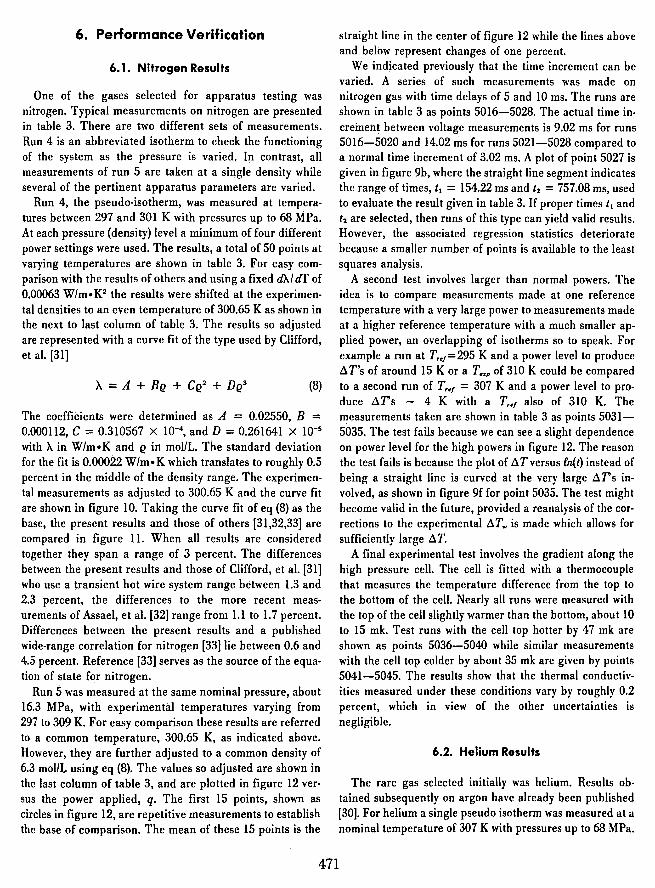
6. Performance Verification

6.1. Nitrogen Results

One of the gases selected for apparatus testing was nitrogen. Typical measurements on nitrogen are presented in table 3. There are two different sets of measurements. Run 4 is an abbreviated isotherm to check the functioning of the system as the pressure is varied. In contrast, all measurements of run 5 are taken at a single density while several of the pertinent apparatus parameters are varied.

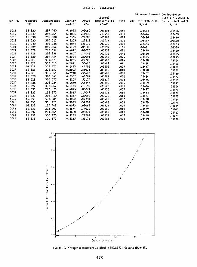
Run 4, the pseudo-isotherm, was measured at tempera­tures between 297 and 301 K with pressures up to 68 MPa. At each pressure (density) level a minimum of four different power settings were used. The results, a total of 50 points at varying temperatures are shown in table 3. For easy com­parison with the results of others and using a fixed dAl cIT of 0.00063 W/m-K2 the results were shifted at the experimen­tal densities to an even temperature of 300.65 K as shown in the next to last column of table 3. The results so adjusted are represented with a curve fit of the type used by Clifford, et al. [31]

(8)

The coefficients were determined as A = 0.02550, B = 0.000112, C = 0.310567 X 10-4

, and D = 0.261641 X 10-5

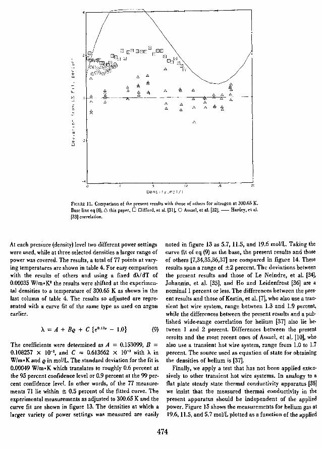
with A in W/m-K and e iIi mol/L. The standard deviation for the fit is 0.00022 W/m-K which translates to roughly 0.5 percent in the middle of the density range. The experimen­tal measurements as adjusted to 300.65 K and the curve fit are shown in figure 10. Taking the curve fit of eq (8) as the base, the present results and those of others [31,32,33] are compared in figure 11. When all results are considered together they span a range of 3 percent. The differences between the present results and those of Clifford, et al. [31] who use a transient hot wire system range between 1.3 and 2.3 percent, the differences to the more recent meas­urements of Assael, et al. [32] range from 1.1 to 1.7 percent. Differences between the present results and a published wide·range correlation for nitrogen [33] lie between 0.6 and 4.5 percent. Reference [33] serves as the source of the equa­tion of state for nitrogen.

Run 5 was measured at the same nominal pressure, about 16.3 MPa, with experimental temperatures varying from 297 to 309 K. For easy comparison these results are referred to a common temperature, 300.65 K, as indicated above. However, they are further adjusted to a common density of 6.3 mol/L using eq (8). The values so adjusted are shown in the last column of table 3, and are plotted in figure 12 ver­sus the power applied, q. The first 15 points, shown as circles in figure 12, are repetitive measurements to establish the base of comparison. The mean of these 15 points is the

471

straight line in the center of figure 12 while the lines above and below represent changes of one percent.

We indicated previously that the time increment can be varied. A series of such measurements was made on nitrogen gas with time delays of 5 and 10 ms. The runs are shown in table 3 as points 5016-5028. The actual time in­crement between voltage measurements is 9.02 ms for runs 5016-5020 and 14.02 ms for runs 5021-5028 compared to a normal time increment of 3.02 ms. A plot of point 5027 is given in figure 9b, where the straight line segment indicates the range of times, tt = 154.22 ms and t2 = 757.08 ms, used to evaluate the result given in table 3. If proper times tt and t2 are selected, then runs of this type can yield valid results. However, the associated regression statistics deteriorate because a smaller number of points is available to the least squares analysis.

A second test involves larger than normal powers. The idea is to compare measurements made at one reference temperature with a very large power to measurements made at a higher reference temperature with a much smaller ap­plied power, an overlapping of isotherms so to speak. For example a run at Tr .. f =295 K and a power level to produce ~T's of around 15 K or a T .. "p of 310 K could be compared to a second run of Tr .. f = 307 K and a power level to pro­duce ~Ts - 4 K with a Tr .. f also of 310 K. The measurements taken are shown in table 3 as points 5031-5035. The test fails because we can see a slight dependence on power level for the high powers in figure 12. The reason the test fails is because the plot of AT versus fn(t) instead of being a straight line is curved at the very large ~Ts in­volved, as shown in figure 9f for point 5035. The test might become valid in the future, provided a reanalysis of the cor­rections to the experimental ATw is made which allows for sufficiently large AT.

A final experimental test involves the gradient along the high pressure cell. The cell is fitted with a thermocouple that measures the temperature difference from the top to the bottom of the cell. Nearly all runs were measured with the top of the cell slightly warmer than the bottom, about 10 to 15 mk. Test runs with the cell top hotter by 47 mk are shown as points 5036-5040 while similar measurements with the cell top colder by about 35 mk are given by points 5041-5045. The results show that the thermal conductiv­ities measured under these conditions vary by roughly 0.2 percent, which in view of the other uncertainties is negligible.

6.2. Helium Results

The rare gas selected initially was helium. Results ob­tained subsequently on argon have already been published [30]. For helium a single pseudo isotherm was measured at a nominal temperature of 307 K with pressures up to 68 MPa.

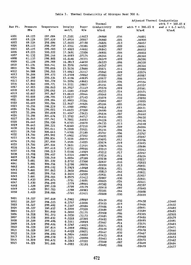
Table 3. Thermal Conductivity of Nitrogen Near 300 K.

Adjusted Thermal Conductivity Thermal with T = 300.65 K

Run Pt. Pressure Temperature Density Power Conductivity STAT with T = 300.65 K and p = 6.3 mol/L MPa K mol/L W/m W/m.K W/m.K W/m.K

4001 69.123 297 .004 17 .5101 .14023 .06868 .034 .06891 4002 69.124 297.439 17.4916 .20067 .06880 .021 .06900 4003 69.124 298.096 17.4635 .27180 .06821 .013 .06837 4004 69.123 298.759 17.4351 .35381 .06829 .009 .06841 4005 69.125 299.583 17.4003 .44662 .06845 .007 .06852 4006 69.125 300.322 17.3691 .55006 .06831 .004 .06833 4007 61.132 298.146 16.4493 .27174 .06344 .012 .06360 4008 61.133 298.905 16.4166 .35371 .06379 .009 .06390 4009 61.128 299.709 16.3813 .44650 .06333 .006 .06339 4010 61.131 300.741 16.3376 .54992 .06347 .005 .06346 4011 54.586 298.026 15.5156 .23468 .05971 .014 .05988 4012 54.588 298.703 15.4863 .31117 .05962 .009 .05974 4013 54.588 299.475 15.4528 .39862 .05980 .007 .05987 4014 54.588 300.334 15.4156 .49695 .05977 .006 .05979 4015 47.903 300.778 14.3096 .49683 .05555 .004 .05554 4016 47.903 299.771 14.3531 .39857 .05551 .006 .05557 4017 47.905 298.863 14.3927 .31119 .05570 .009 .05581 4018 47.905 298.042 14.4285 .23469 .05555 .014 .05571 4019 40.607 297.907 13.0618 .20044 .05049 .016 .05066 4020 40.608 298.705 13.0277 .27163 .05078 .010 .05090 4021 40.609 299.584 12.9903 .35361 .05092 .007 .05099 4022 40.609 300.704 12.9427 .44624 .05104 .005 .05104 4023 33.596 298.229 11.4980 .20061 .04616 .015 .04631 4024 33.596 299.023 11.4655 .27208 .04600 .010 .04610 4025 33.596 300.028 11.4247 .35423 .04636 .007 .04640 4026 33.596 301.176 11.3782 .44717 .04633 .005 .04630 4027 26.643 297.741 9.7001 .14033 .04128 .023 .04146 4028 26.642 298.530 9.6705 .20078 .04135 .013 .04148 4029 26.643 299.522 9.6340 .27210 .04199 .009 .04206 4030 26.642 300.611 9.5939 .35421 .04154 .006 .04154 4031 19.700 300.643 7.4708 .31180 .03707 .006 .03707 4032 19.700 299.992 7.4902 .27212 .03693 .008 .03697 4033 19.700 298.934 7.5221 .20073 .03695 .012 .03706 4034 19.700 297.950 7.5521 .14029 .03678 .019 .03695 4035 19.700 297.532 7.5651 .11414 .03676 .026 .03696 4036 12.708 297.418 5.0731 .09066 .03223 .035 .03243 4037 12.708 298.319 5.0546 .14029 .03212 .017 .03227 4038 12.708 299.457 5.03i4 .20079 .03216 .011 .03224 4039 12.708 300.749 5.0054 .27209 .03238 .008 .03237 4040 5.681 301.332 2.2732 .23508 .02837 .0lQ .02833 4041 5.681 300.556 2.2798 .20076 .02830 .013 .02831 4042 5.681 299.102 2.2923 .14028 .02816 .021 .02826 4043 5.681 297.843 2.3032 .09064 .02813 .042 .02831 4044 5.681 299.714 2.2870 .16920 .02821 .016 .02827 4045 5.681 298.464 2.2975 .11412 .02807 .030 .02821 4046 1.430 299.675 .5751 .14031 .02605 .024 .02611 4047 1.430 298.299 .5779 .09064 .02582 .041 .02597 4048 1.429 297.129 .5799 .05179 .02618 .097 .02640 4049 1.429 297.703 .5788 .06983 .02581 .064 .02600 4050 1.429 298.984 .5761 .11411 .02608 .030 .02618 5001 16.327 297.649 6.3985 .09069 .03439 .032 .03458 .03440 5002 16.327 298.523 6.3757 .14036 .03453 .019 .03466 .03452 5003 16.327 299.492 6.3507 .20084 .03484 .011 .03491 .03482 5004 16.327 300.657 6.3209 .27209 .03489 .007 .03489 .03485 5005 16.327 301.440 6.3010 .31171 .03508 .006 .03503 .03503 5006 16.328 301.373 6.3030 .31172 .03485 .006 .03480 .03479 5007 16.328 300.632 6.3218 .27203 .03495 .006 .03495 .03491 5008 16.329 299.496 6.3511 .20069 .03467 .011 .03474 .03465 5009 16.329 298.426 6.3787 .14025 .03471 .018 .03485 .03471 5010 16.329 297.614 6~3999 .09061 .03459 .035 .03478 .03460 5011 16.329 297.512 6.4028 .09071 .03447 .032 .03467 .03448 5012 16.329 298.293 6.3824 .14037 .03453 .018 .03468 .03453 5013 16.329 299.270 6.3571 .20090 .03463 .011 .03472 .03462 5014 16.329 300.472 6.3263 .27222 .03468 .007 .03469 .03464 5015 16.329 301.184 6.3083 .31195 .03482 .006 .03479 .03477

472

Run Pt. Pressure MPa

5016 16.330 5017 16.330 5018 16.330 5019 16.330 5020 16.330 502l 16.329 5022 16.329 5023 16.329 5024 16.329 5025 16.329 5026 16.329 5027 16.329 5028 16.329 5031 16.328 5032 16.328 5033 16.328 5034 16.328 5035 16.327 5036 16.333 5037 16.333 5038 16.333 5039 16.333 5040 16.333 5041 16.337 5042 16.337 5043 16.337 5044 16.338 5045 16.338

Table 3. (Continued)

Adjusted Thermal Condu~tivity Thermal

Temperature Density Power Conductivity STAT with T ~ 300.65 K K mo1/L W/m W/m.K W/m.K

297.460 6.4043 .09069 .03505 .060 .03525 298.264 6.3834 .14035 .03459 .033 .03474 299.300 6.3566 .20085 .03481 .019 .03490 300.512 6.3255 .27213 .03476 .0l2 .03477 301.228 6.3074 ~3ll79 .03470 .009 .03466 296.862 6.4199 .05183 .03397 .186 .03421 297.554 6.4017 .09073 .03459 .081 .03479 298.358 6.3807 .14043 .03436 .041 .03450 299.454 6.3524 .20091 .03447 .024 .03455 300.573 6.3235 .27225 .03468 .014 .03468 302.013 6.2871 .35420 .03497 .011 .03488 303.570 6.2483 .44706 .03505 .009 .03487 305.150 6.2095 .55073 .03486 .010 .03458 301.848 6.2910 .35473 .03465 .008 .03457 303.341 6.2537 .44782 .03481 .006 .03464 305.077 6.2109 .55174 .03514 .005 .03486 306.934 6.1660 .66648 .03509 .004 .03469 308.967 6.1175 .79195 .03528 .003 .03476 297.573 6.4025 .09074 .03478 .037 .03497 298.377 6.3815 .14047 .03471 .019 .03485 299.450 6.3537 .20096 .03479 .011 .03487 300.685 6.3222 .27231 .03488 .007 .03488 301.270 6.3073 .31209 .03483 .006 .03479 297.448 6.4073 .09066 .03435 .034 .03455 298.207 6.3874 .14029 .03464 .019 .03479 299.265 6.3600 .20074 .03469 .Oll .03478 300.475 6.3293 .27202 .03477 .007 .03478 301.173 6.3ll5 .3ll71 .03483 .006 .03480

7.2.-------------------__ --__________________ --------~ x 10. 2

6.4

y: 5.6

E "-~

> 4.8

U ::J

U C o u - 4.0 co E '­C1l .c. t-

3.2

/< ~/

./ /'

/

I

/

/ /

I . .

2.4L-__________ --________ --__________________ ------__ ~

o 12 16

DgnSl ty.mOI/I

FIGURE 10. Nitrogen measurements shifted to 300.65 K with curve fit, eq (8),

473

with T • 300.65 K and p • 6.3 mo1/L

W/m·K

.03506

.03459

.03480

.03472

.03465

.03399

.03460

.03435

.03445

.03464

.03490

.03496

.03474

.03459

.03472

.03502

.03493

.03509

.03478

.03470

.03477

.03484

.03478

.03435

.03463

.03467

.03473

.03478

-c OJ u '-OJ 0. 6. 6. 6.

u.. ~ (f) 6. -l 6. 6. E 0

~ '-

~ ~

b 6. 6. ~

6. 6. ~ 6. ~

6. 6.

6. 6. 6. 6. 6. S}

*' 6.

c 0

6.

-ro

> OJ -2 0

-4 L------+----~------12-----I:+:-o------:2C1

DenSlty.mOI/I

FIGURE 11. Comparison of the present results with those of others for nitrogen at 300.65 K. Base line eq (8), b. this paper, 0 Clifford, et a1. [31],0 Assael, et a1. [32]. - Hanley, et a1.

[33] correlation.

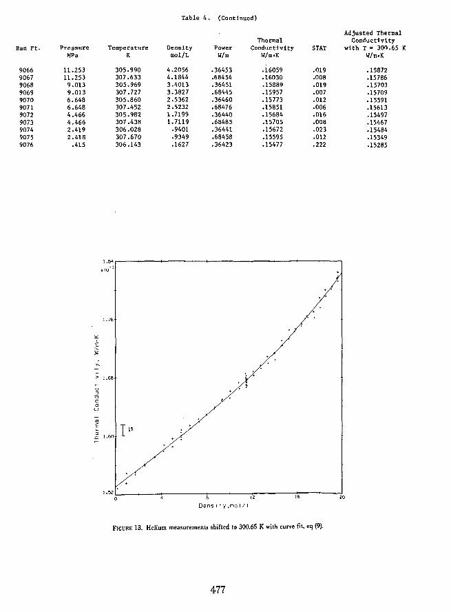
At each pressure (density) level two different power settings were used, while at three selected densities a larger range of power was covered. The results, a total of 77 points at vary­ing temperatures are shown in table 4. For easy comparison with the results of others and using a fixed dAI dT of 0.00035 W/m.K2 the results were shifted at the experimen­tal densities to a temperature of 300.65 K as shown in the last column of table 4. The results so adjusted are repre­sented with a curve fit of the same type as used on argon earlier.

A = A + Be + C {eo. Up - 1.0} (9)

The coefficients were determined as A = 0.153099, B = 0.108257 X 10-1, and C = 0.613662 X 10-3 with A in W/m.K and e in mol/L. The standard deviation for the fit is 0.00049 W/m.K which translates to roughly 0.6 percent at the 95 percent confidence level or 0.9 percent at the 99 per­cent confidence level. In other words, of the 77 measure­ments 71 lie within ± 0.5 percent of the fitted curve. The experimental measurements as adjusted to 300.65 K and the curve fit are shown in figure 13. The densities at which a larger variety of power settings was measured are easily

noted in figure 13 as 5.7, H.5, and 19.6 mollL. Taking the curve fit of eq (9) as the base, the present results and those of others [7,34,35,36,37] are compared in figure 14. These results span a range of ±2 percent. The deviations between the present results and those of Le N eindre, et al. [34J, Johannin, et a1. [35], and Ho and Leidenfrost [36] are a nominal 1 percent or less. The differences between the pres· ent results and those of Kestin, et al. [7J, who also use a tran· sient hot wire system, range between 1.3 and 1.9 percent, while the differences between the present results and a pub· lished wide-range correlation for helium [37] also lie be· tween 1 and 2 percent. Differences between the present results and the most recent ones of Assael, et a}. [10], who also use a transient hot wire system, range from 1.0 to 1.7 percent. The source used as equation of state for obtaining the densities of helium is [37].

Finally, we apply a test that has not been applied exten· sively to other transient hot wire systems. In analogy to a flat plate steady state thermal conductivity apparatus [38J we insist that the measured thermal conductivity in the present apparatus should be independent of the applied power. Figure 15 shows the measurements for helium gas at 19.6, 11.5, and 5.7 mol/L plotted as a function of the applied

474

3.64

> 3.48

u :J

U C o

U

- 3.40 co E '­OJ £. I-

3.32

3.24

0.0

( t

~

i I~ t~ t

+

,~

!~ I P ~~

.2 .4 .6 .8

Heat Flux, W/m

FIGURE 12. Measured thermal conductivity as a function of the applied power. Apparatus tests with nitrogen gas. o normal measurements, D. cell top cold, V cell top hot o 5 ms delay, time increment 9.02 ms ¢ 10 ms delay, time increment 14.02 ms * larger than normal powers.

power. Whereas q changes by a factor of nearly five no dependence of the measured conductivity on power level is discernible. For reference, the values of the curve fit (eq (9» plus or minus 0.5 percent are shown as three straight lines for each density in figure IS. The error bars for each point are those originating from the regression straight line fit for each point, see column STAT in table 4.

6.3. Cell Alinement

During the construction of the apparatus we sought to keep the cell in vertical alinement to insure that convection in the cell would be delayed as long as possible. Later we sought to verify the alinement by a series of experimental measurements, some 162 points with oxygen gas as a sample at a pressure near 10 MPa and a temperature of around 240 K. The position of each cell alinement screw was varied in turn by a measured amount. For each setting of the screws a series of seven to nine measurements were taken varying the

applied power, q. If the cell is out of alinement the measured thermal conductivity increases. The increase is more pronounced at the higher power levels. The proper setting for the alinement screws occurs when the measured results are most nearly independent of q as illustrated in figure IS. The final settings chosen were nearly identical to those first achieved during construction of the apparatus. In fact, the measurements on helium, Run No.9, were taken four months before the series on alinement, Run No. 19.

6.4. Other Tests

Tests were run on nitrogen gas at room temperature with only a single hot wire in the bridge. The circuit was rewired so that either R. or R3 , see figure 2, were replaced by yet another 100 {} standard resistor. The data reduction pro­gram had to be modified accordingly. The results were eval­uated only on the minicomputer, and are relative to similar

475

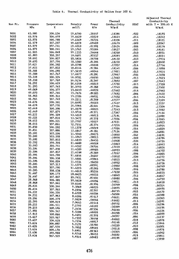
Table 4. Thermal Conductivity of Helium Near 300 K.

Adjusted Thermal Thermal Conductivity

Run Pt. Pressure Temperature Density Power Conductivity STAT with T ~ 300.65 K MPa K mo1/L W/m W/m.K W/m.K

9001 63.980 306.154 19.6780 .36457 .18386 .022 .18193 9002 63.978 306.459 19.6629 .46029 .18445 .014 .18242 9003 63.978 306.788 19.6469 .56726 .18336 .Oll .18121 9004 63.979 307.287 19.6229 .68489 .18479 .009 .18247 9005 63.979 307.741 19.6010 .81392 .18424 .006 .18176 9006 63.979 308.241 19.5769 .95386 .18427 .005 .18161 9007 61.905 306.849 19.1335 .56688 .18268 .010 .18051 9008 61.905 308.397 19.0601 .95337 .18285 .005 .18014 9009 59.692 306.827 18.5826 .56708 .18132 .010 .17916 9010 59.693 307.794 18.5380 .81386 .18250 .007 .18000 9011 57.621 306.382 18.0798 .46038 .17957 .014 .17756 9012 57.622 307.822 18.0144 .81384 .18141 .006 .17890 9013 55.588 306.292 17.5633 .46046 .178ll .015 .17614 9014 55.588 307.767 17.4977 .81391 .17947 .006 .17698 9015 53.338 306.324 16.9781 .46030 .17822 .015 .17623 9016 53.338 307.769 16.9154 .81397 .17892 .007 .17643 9017 51.292 306.429 16.4358 .46023 .17730 .015 .17528 9018 51.293 307.763 16.3793 .81388 .17749 .006 .17500 9019 49.069 306.377 15.8453 .46028 .17662 .014 .17462 9020 49.070 307.784 15.7876 .81385 .17682 .006 .1743Z 9021 46.963 306.311 15.2786 .46031 .17652 .015 .17454 9022 46.964 307.749 15.2211 .81389 .17577 .006 .17329 9023 44.676 306.361 14.6495 .46023 .17437 .013 .17237 9024 44.678 307.731 14.5966 .81401 .17554 .006 .17306 9025 42.449 306.396 14.0279 .46025 .17243 .013 .17042 9026 42.449 307.874 13.9726 .81371 .17387 .006 .17134 9027 40.222 306.328 13 .4010 .46013 .17191 .014 .16992 9028 40.222 307.816 13 .3472 .81378 .17336 .006 .17085 9029 38.053 306.321 12.7787 .46027 .17121 .013 .16923 9030 38.053 307.861 12.7251 .81376 .17216 .006 .16964 9031 35.850 306.292 12.1378 .46029 .17026 .014 .16829 9032 35.851 307.886 12.0847 .81381 .17134 .006 .16881 9033 33.592 305.206 11.5040 .20675 .16850 .042 .16691 9034 33.592 305.508 11.4943 .28015 .16954 .029 .16784 9035 33.592 305.853 11.4833 .36455 .16908 .020 .16726 9036 33.592 306.306 11.4688 .46028 .16863 .014 .16665 9037 33.593 306.741 11.4552 .56704 .17039 .010 .16826 9038 33.594 307.256 11.4389 .68485 .16933 .008 .16702 9039 33.594 307.857 11.4198 .81389 .17057 .006 .16805 9040 33.594 305.799 11.4856 .36407 .16952 .020 .16772 9041 33.594 306.338 11.4684 .45965 .16955 .013 .16756 9042 33.595 306.824 11.4531 .56620 .16952 .011 .16736 9043 33.595 307.313 1l.4375 .68391 .16982 .008 .16749 9044 33.595 307.790 11.4223 .81285 .17030 .006 .16780 9045 33.595 308.438 1l.4018 .95255 .17128 .005 .16855 9045 31.497 306.173 10.8425 .46033 .16840 .013 .16647 9046 31.497 307.807 10.7931 .81402 .16980 .006 .16730 9047 28.968 306.381 10.0629 .46036 .168ll .013 .16610 9048 28.968 307.941 10.0184 .81396 .16769 .006 .16514 9049 26.634 306.344 9.3369 .46035 .16695 .014 .16496 9050 26.634 307.965 9.2936 .81397 .16735 .005 .16479 9051 24.532 306.354 8.6709 .46038 .16588 .014 .16388 9052 24.532 307.963 8.6306 .81417 .16621 .006 .16365 9053 22.396 306.379 7.9829 .46046 .16482 .013 .16281 9054 22.395 308.019 7.9445 .81418 .16552 .006 .16294 9055 20.255 306.511 7.2793 .46102 .16399 .013 .16194 9056 20.255 308.186 7.2434 .81536 .16490 .006 .16226 9057 17 .991 306.347 6.5288 .46009 .16298 .014 .16099 9058 17 .913 308.066 6.4692 .81378 .16397 .006 .16137 9059 15.627 305.967 5.7333 .36458 .16262 .018 .16076 9060 15.627 306.425 5.7254 .46017 .16148 .012 .15946 9061 15.626 306.897 5.7170 .56700 .16220 .010 .16001 9062 15.626 307.578 5.7052 .68465 .16218 .008 .15976 9063 15.626 308.170 5.6951 .81363 .16305 .006 .16042 9064 13.436 305.988 4.9748 .36453 .16032 .019 .15841 9065 13.436 307.519 4.9516 .68483 .16199 .007 .15959

476

Run Pt. Pressure MPa

9066 11.253 9067 11.253 9068 9.013 9069 9.013 9070 6.648 9071 6.648 9072 4.466 9073 4.466 9074 2.419 9075 2.418 9076 .415

Table 4. (Continued)

Thermal Temperature Density Power Conductivity STAT

K mol/L W/m W/m.K

305.990 4.2056 .36453 .16059 .019 307.633 4.1844 .68454 .16030 .008 305.969 3.4013 .36451 .15889 .019 307.727 3.3827 .68445 .15957 .007 305.860 2.5362 .36460 .15773 .012 307.452 2.5232 .68476 .15851 .006 305.982 1.7199 .36440 .15684 .016 307.438 1.7119 .68485 .15705 .008 306.028 .9401 .36441 .15672 .023 307.670 .9349 .68458 .15595 .012 306.143 .1627 .36423 .15477 .222

1.84,..------_+_------+----_1---_---+------,

x 10. 1

1. 76

> 1.68

U :::J TI C a

U

..

Adjusted Thermal Conductivity

with T .. 300.65 W/m.K

.15872

.15786

.15703

.15709

.15591

.15613

.15497

.15467

.15484

.15349

.15285

1.52 oL.-----+-----~-------:1'::"2-----;+;:16-----!20.

Dens I I Y ,mo I / I

FIGURE 13. Helium measurements shifted to 300.65 K with curve fit, eq (9).

477

K

c: <ll U

<ll Q

u.. (f)

.....J

to o

c: o

>

0 0 0

6 (}:,

00 00

8. 0 0

8. 8.8. ~

8.

(}:,

<ll -2 o

-4L-________ -+ __________ ~----______ ~----__ --~~--------~

o 8 12 16 20

DenSlty.mol/l

FIGURE 14. Comparison of the present results with those of others for helium at 300.65 K. Base line eq (9), b. this paper, 0 Kestin, et aJ. [7], <> Le Neindre, et aJ. [34], • Johannin, et aJ. [35], 0 Ho and Leidenfront 136], - McCarty [37] correlation.

1.88

.10 I

I.eo

> 1.72

U ::J

U C o

U

co E

1.56

curvefit va J ue ({)

curvef; t value (

-ID (U

T curvefl t value ~

( "

1

1 19.6 mol/L t

l' (f\ rh I I -r

t ~l. 5 mol/L rh

1 ffi f )R -r !

5.7 mol/l . 1 T CD 'Ii ! 1

0.0 .2 .4 .6 .8 1.0

Heat Flux, W/m

FIGURE 15. Measured thermal conductivity as a function of the applied power. Apparatus test with helium gas.

478

measurements made the same day with the full bridge. The apparent conductivities for the single wires increase above those of the full bridge as follows

full bridge long hot wire only short hot wire only

1.000 1.048 1.083.

Measurements of this type show the relative effect of the end corrections which 'Yould be required for the single wire, but which are presumed to be off setting in tpe bridge circuit.

7. Errors

Precision, reproducibility, internal consistency, and accu­racy are discussed here.

Precision. The measurement vanatIOn in the voltages across the Wheatstone bridge is ±28 p. V which corresponds to about 25 mK. The effective errors in the experimental AT values are 6 percent for the very small power levels, i.e., a final tlT of about 0.5 K, to 0.4 percent for a final tlT of about 6 K. An example of the distributio~ of the exper­imental tlrs about the calculated straight line was shown in figure 8b. The regression program accounts for the spread in measurements by assigning a variance to the coefficients of the calculated straight line. The value STAT as printed in tables 3 and 4 is the fractional error in the slope of the straight line obtained from the variance in the slope (2u) divided by by the slope itself. The value STAT is the primary measure of the experimental precision because other contributions such as an error in q are quite negligi­ble. For final tlT values of 3.5 K or more which includes about 70 percent of all measurements made to date the nominal precision (2u) is 0.6 percent or slightly less.

Reproducibility was tested by measuring (a) repeatedly the same point at the same fluid conditions on a given day, (b) by measuring similar points at different power levels, and (c) by repeating different isotherms at different times some months apart. Examples of (a) are found in table 3, examples of (b) are given in the sections on nitrogen and helium. For (c), isotherms at 160 K, 200 K, and 240 K were repeated during the measurements on oxygen [26].

Internal consistency. When measurements are made over a large portion of the thermal conductivity surface, and if an analytical function is used to represent the surface, then it becomes possible to check the internal consistency of the set of measurements by intercomparing the deviations and deviation patterns for the various isotherms. Such checks are possible for both propane [27] and oxygen [26]. In pro-

pane seven different liquid isotherms can be represented with an overall deviation of 1.2 percent (2u). For oxygen, 13 isotherms from the surface which includes gas, liquid, sub­critical vapor and the near critical region for an average deviation of 1.6 percent.

Accuracy. The accuracy of the measurement can in prin­ciple be estab~ished from the measurements and certain theoretical considerations, i.e., for the rare gases the Eucken factor [7]. For argon [30] the 0.3 percent obtained in the low density extrapolation was considered a fortunate coincidence and an overall accuracy of ± 1 percent was claimed. For the results on helium in table 4 the low density extrapolation yields a result which is 1.8 percent low. Accu­racy can also be estimated by comparison to the results of others. For the present apparatus these intercomparisons cover a- wide range of fluids, and a wide range of pressures, densities and temperatures. Summarized these comparisons are:

Nitrogen: this apparatus is 1.3 to 2.3 percent lower than other authors [31,32,33].

Helium: this apparatus is 1. to 1.8 percent lower than other authors [7,34,35,36,37].

Argon: this apparatus is 1. percent lower than other authors [30].

Oxygen: this apparatus is 1-2 percent lower than other authors [26].

Propane: this apparatus is higher at some densities, lower at other densities when compared to other authors [27].

Hydrogen: this apparatus is 1.5 percent lower than other authors [39].

8. Summary

A new transient hot wire thermal conductivity apparatus for fluids has been developed. It differs from some of the other transient hot wire systems in that it uses compen­sating wires in a Wheatstone bridge arrangement. It differs from th~se transient hot wire systems that use a bridge in that the voltages developed across the bridge are measured directly. The apparatus is a very rapid measuring device. Sixty points, a full pseudo-isotherm, are possible in a day. The system is capable of measuring a wide range of fluid temperatures, densities, and pressures. Fluid states, such as dilute gas, dense gas, the near critical states, vapor at tem­peratures below critical, compressed liquid states, and metastable liquid states at densities below saturation, are accessible for many liquefied gases. A wide variety of simple fluids has been measured in the system so far. It appears that the precision of the new system is on the order of 0.6 percent while its accuracy is close to 1.5 percent.

479

9. References

[IJ Pittman, J. F. T. Fluid thermal conductivity determination by the transient line source method. Thesis. University of London; Lon· don; 1968.

[2] Haarman, J. W. Thesis. Technische Hogeschool; Delft; 1969. [3J Mani, N. Precise determination of the thermal conductivity of fluids

using absolute transient hot·wire technique. Thesis. University of Calgary. Calgary, Alberta, Canada. 1971 Aqgust.

[4J de Groot, J. J.; Kestin, J.; Sookiazian, H. Instrument to measure the thermal conductivity of gases. Physica. 75: 454-482; 1974.

[5J Healy, J. J.; de Groot, J. J.; Kestin, J. The theory of the transient hot· wire method for measuring thermal conductivity. Physica 82Q2): 392-408; 1976 April.

[6J de Groot, J. J.; Kestin, J.; Sookiazian, H. The thermal conductivity of four monatomic gases as a function of density near room temperature. Physica. 92A: 117-144; 1978.

[7] Kestin, J.; Paul, R.; Clifford, A. A.; Wakeham, W. A. Absolute determination of the thermal conductivity of the noble gases at room temperature up to 35 MPa. Physica looA(2): 349-369; 1980 February.

[8J Kestin, J.; Wakeham, W. A. A contribution to the theory of the tran· sient hot·wire technique for thermal conductivity measurements. Physica. 92A(1 and 2): 102-116; 1978 June.

[9] Clifford, A. A.; Kestin, J.; Wakeham, W. A. A further contribution to the theory of the transient hot·wire technique for thermal conduc­tivity measurements. Physica. looA(2): 370-374; 1980 February.

[10] Assael, M. J.; Dix, M.; Lucas, A.; Wakeham, W. A. Absolute deter· mination of the thermal conductivity of the noble gases and two of their binary mixtures. J. Chem. Soc., Faraday Trans. 77(1): 439-464; 1981.

[11] Menashe, J.; Wakeham, W. A. 'Absolute messurements of the thermal conductivity of liquids of pressures up to 500 MPa. to be published, Physica.

[12] de Castro, C. A. Nieto; Cal ado, J. C. G.; Wakeham, W. A.; Dix, M. An apparatus to measure the thermal conductivity of liquids. Journal of Physics E: Scient. Inst. 9: 1073-1080; 1976.

[13] de Castro, C. A. Nieto; Calado, J. C. G.; Wakeham, W. A. Absolute measurements of the thermal conductivity of liquids using a tran· sient hot·wire technique. Cezarilyan, A. ed. Proceedings of the seventh symposium on thermophysical properties; 1977 May 10-12; Gaithersburg, Maryland; New York; ASME; 1977; 730-738.

[14] Carslaw, H. S.; Jaeger, J. C. Conduction of heat in $olids. 2nd Ed. Ox· ford: University Press; 1959. 510 p.

[15] Riddle, J. L.; Furukawa, G. T.; Plumb, H. H. Platinum Resistance Ther· mometry. Nat. Bur. Stand. (U.S.) Mo'nogr. 126; 1973 April. 129 p.

[16] Lyman, T., ed. Metals Handbook. 8th Ed. Vol I. Properties and Selec­tion of Metals. American Society for Metals. Metals Park, Ohio; 1969 September. 1300 p.

[17] Younglove, B. A. Speed of sound in fluid parahydrogen. J. Acoust. Soc. Am. ~3): 433-438; 1965 September.

[18] Diller, D. E. Measurements of the viscosity of parahydrogen. J. Chem. Phys. -12(6): 2089-2100; 1965 March 15.

[19] Weber, L A. Density and compressibility of oxygen in the critical region. Phys. Rev. A 2(6): 2379-2388; 1970 December.

[20] Haynes, W. M.; Hiza, M. J.; Frederick, N. V. Magnetic suspension densimeter for measurements on fluids of cryogenic interest. Rev Sci. Instrum. 47(10): 1237-1250; 1976 October.

[21] Straty, G. C.; Younglove, B. A. A fluorine compatible low temperature electrical feed through. Rev. Sci. Instrum. 43(1): 156-157; 1972 January..

[22] Key, C. F. Compatibility of materials with liquid oxygen, III. National Aeronautics and Space Administration, Marshall Space Flight Center, Huntsville, Ala; Tech. Memo X67-10596; 1966 November.

[23] Bankaitis, H.; Schueller, C. F. ASRDI Oxygen technology survey Volume II: cleaning requirements, procedures, and verification techniques. National Aeronautics and Space Administration Special Publication SP-3072; 1972. 76 p.

[24] Goodwin, R. D. Apparatus for determination of pressure-density·tem· perature relations and specific heats of hydrogen to 350 at· mospheres at temperatures above 14 K. J. Res. Nat. Bur. Stand. (U.S.) 65Q4): 231-243; 1961 October·December.

[25] Goodwin, R. D. An improved l{C power regulator. Timmerhaus, K. D., ed. Advances in Cryogenic Engineering. Proceedings of the 1959 Cryogenic Engineering Conference. Plenum Press Inc., New York; 1960. 577-579.

. [26] ltoder, H. M. The thermal conductivity of oxygen. J. Res. Nat. Bur. Stand. (U.S.). to be published.

[27] Roder, H. M.; de Castro, C. A. N. Thermal conductivity of liquid pro­pane. Submitted to J. Chern. Engr. Data.

[28] Hall, L. A~ Survey of electrical resistivity measurements on 16 pure metals in the temperature range 0 to 273 K. Nat. Bur. Stand. (U.S.) Tech. Note 365; 1968 February. 111 p.

[29] de Castr'o, C, A. Nieto; Wakeham, W. A. Experimental aspects of the transient hot~wire technique for thermal conductivity measurements. Mirkovich, V. V. ed. Thermal conductivity 15. 1977 August 24-26; Ottawa, Ontario, Canada; New York; Plenum Pub!. Corp.; 1978; 235-243.

[30] de Castro, C. A. N.; Roder, H. M. Absolute determination of the ther· mal conductivity of argon at room temperature and pressures up to 68 MPa. J. Res. Nat. Bur. Stand. (U.S.). 86(3): 293-307; 1981 May· June.

[31] Clifford, A. A.; Kestin, J.; Wakeham, W. A. Thermal conductivity of N2, CH4, and CO2 at room temperature and at pressures up to 35 MPa. Physica. 97A(2): 287-295; 1979 July ..

[32] Assael, M. J.; Wakeham, W. A. Thermal conductivity of four poly· atomic gases. J. Chem. Soc., Faraday Trans. 77(1): 697-707; 1981.

[33] Hanley, H. J. M.; McCarty,H. D.; Haynes, W. M. The viscosity and thermal conductivity for dense gaseous and liquid argon, krypton, xenon, nitrogen. and oxygen. J. Phys. Chern. Ref. Data 3(4): 979-1017; 1974.

[34] LeNeindre, B.;,Bury,P.; Tufeu, R.; Johannin, P.; Vodar, B. Recent developments at Bellevue on thermal conductivity measurements of compressed gases. Flynn, D. A.; Peavy, B. A., Jr. ed. Thermal con· ductivity; Proceedings of the seventh conference; 1967 November 13-16; Gaithersburg, Maryland. Nat. Bur. Stand. (U.S.) Spec. Pub!. 302; 1968 September. 579-593.

[35] Johannin, P.; Wilson, M.; Vodar, B. Heat conductivity of helium at elevated temperatures. Masi, J. F.; Tsai, D. H. ed. Progress in Inter· national Research on Thermodynamic and Transport Properties, Academic Press, New York. 1962.41-8-433.

[36] Ho, C. W.; Leidenfrost, W. Precise determination of the thermal con· ductivity of helium gas at high pressures and moderate temperatures. Grigull, U.; Hahnl, E. eds. Progress in Heat and Mass Transfer. Pergamon Press, Oxford; 1969.55-98.

[37] McCarty, RD. Thermophysical properties of helium4 from 2 to 1500 K with pressures to 1000 atmospheres. Nat. Bur. Stand. (U.S.) Tech. Note 631; 1972 November. 161 p.

[38] Roder, H. M.; DilIer, D. E. Thermal conductivity of gaseous and liquid hydrogen. J. Chem. Phys. 52(11): 5928-5949; 1970 June 1.

[39] Roder, H. M. Thermal conductivity of normal hydrogen. Presented at the 17th International Thermal Conductivity Conference. Gaithers­burg, Maryland; 1981 June 15-18.

480

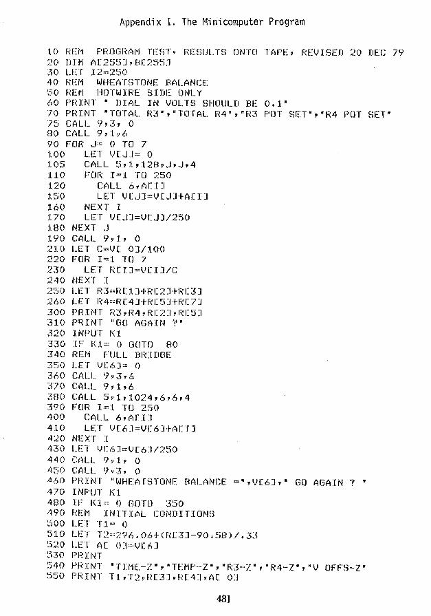
Appendix I. The Minicomputer Program

10 REM PROGRAM TEST, RESULTS ONTO TAPE, REVISED 20 DEC 79 20 DIM A[255J,B[255J 30 LET 12::::2~':;O

40 REM WHEATSTONE BALANCE 50 REM HOTWIRE SIDE ONLY 60 PRINT U DIAL IN VOLTS SHOULD BE 0.1" 70 PRINT "TOTAL R3"y"TOTAL R4","R3 POT SETft,·R4 POT SET­is CALL. <», ~~, 0 80 CALL <] 'J :l v 6 90 F(]l:~ • .1:::: 0 TO 7 100 LET VEJJ= 0 105 CALL 5,1,128vJ,J,4 110 FOR 1=1 TO 250 120 CALL 6,AEIJ 150 LET V[JJ=V[JJtA[IJ 160 NEXT I :L 70 LET V[ . .J]::::V[J]/2~jO :tao NEXT J :L90 CALI... 951t, () 210 LET C=VE 0]/100 220 FOR I:::: 1 TO "7 230 LET R[I]=VCIJ/C 240 NEXT I 250 LET R3=R[tJ+R[2J+R[3J 260 LET R4=R[4J+R[SJtR[7J 300 PRINT R3,R4,R[2],R[SJ 310 PRINT "GO AGAIN 1· 320 :r NPUT 1\:1. 330 IF Kl= 0 GOlD 80 340 REM FULL BRIDGE :3~~jO LET V[6]:::: 0 ~,6() CALI... 9!1 ~:~ , 6 3'70 CALL <],:\.,6 380 CALL 5,1,1024,6,6,4 390 FOR 1=1 TO 250 400 CALL 6,A[IJ 410 LET V[6J=V[6JtAEI] 420 NEXT I 4:~() LET V[6J::::V[fJ]/2S0 44() Ci='-lLL 9,:/. y 0 4~:;O C(')LL 9 If :.3, 0 ~60 PRINT "WHEATSTONE BALANCE =",V[6],M GO AGAIN 1 • 470 INPUT K:l 480 IF Kl= 0 GOIO 350 490 REM INITIAL CONDITIONS ~;:;(}() LET T:I.:::: () 51 () LET T 2 :::: ~? 9/) • () 6 + ( f\ L :3 ::I - 9 () • ~) 8 ) I + :,3 ~)20 LET A[ ()];:::~)[6]

::i30 PF: I NT 540 PRINT nTIME-ZU~"TEMP-Z·,"R3-Z·,·R4-Z·,"V OFFS-Z· 550 PRINT Tl,T2,R[3],R[4],A[ 0]

48]

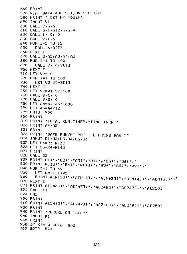
560 PRINT 570 REM DATA AOUISITION SECTION 580 PRINT R SET HP POWER-590 INPUT V1 600 CALL 9,3,6 610 CALL 5,1,512,6,6~9 620 CALL 1, 0, 0 630 CALL 9,1,6 640 FOR 1=1 TO 12 650 CALL 6,A[IJ 660 NEXT I 670 CALL 2,A2,A3,A4~A5 680 FOR 1=1 TO 100 690 CALL 7, O,B[I] 700 NEXT I 710 LET V2= 0 720 FOR 1=1 TO 100 730 LET V2=V2tB[I] 740 NEXT I 750 LET V2=Vl-V2/100 760 CALL 9,1, 0 770 CALL 9,3, 0 780 LET A4=A4tA5/1000 790 LET A5=A4/12 795 GOTO 900 800 PRINT 810 PRINT ·TOTAl RUN TIME·,·TIME INeR •• 820 PRINT A4,A5 821 PRINT 823 PRINT -DATE RUN/PT PRT - l PRESS BAR 1-824 INPUT 01,02,03,04,05,06 825 LET S4=R3-R[3] 826 LET S5=R4-R[4] 827 PRINT 828 CALL 22 829 PRINT 01;-,·02;-,-03;.,-04;-,-05;-,-06;-,-830 PRINT R[3];-,-S4;-,aR[4];-,-S5;a,.A5;-,-V2;a,-840 FOR 1=1 TO 49 850 LET N=(I-l)*5 860 PRINT A[Ntl];-,.A[Nt2];a,-A[Nt3];-,aA[Nt4];a,-A[Nt5];-" 870 NEXT I 871 PRINT A[246];-,-A[247];a,aA[248];.,-A[249];-,8A[250] 872 CALL 11 874 END 900 PRINT 910 PRINT A[246];a,-A[247];"HA[248];.,8A[249];_,8A[250] 920 PRINT 9~0 PRINT ·RECORD ON TAPE1-940 INPUT Kl 945 PRINT 950 IF Kl= 0 GOTO 800 960 GOTO 874

482

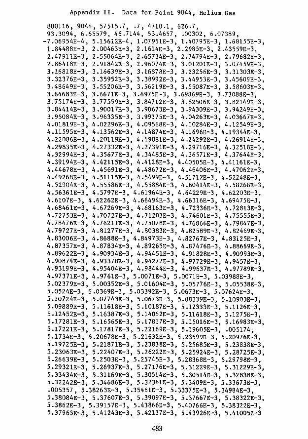
Appendix II. Data for Point 9044, Helium Gas

800116,9044,57515.7, .7,4710.1,626.7, 93.3094,6.65579,46.7144,53.4657, .00302,6.07389,

-7.06954E-4, 5.15612E-4, 1.07951E-3, 1.40795E-3, 1.68155E-3, 1.84488E-3, 2.00463E-3, 2.1614E-3, 2.2985E-3, 2.43559E-3, 2.47911E-3, 2.55064E-3, 2.65734E-3, 2.74794E-3, 2.79682E-3, 2.86418E-3, 2.91842E-3, 2.96074E-3, 3.01201E-3, 3.07459E-3, 3.16818E-3, 3.16639E-3, 3.16878E-3, 3.23256E-3, 3.31303E-3, 3.32376E-3, 3.35952E-3, 3.38992E-3, 3.44953E-3, 3.45609E-3, 3.48649E-3, 3.55206E-3, 3.56219E-3, 3.55087E-3, 3.58603E-3, 3.64683E-3, 3.6671E-3, 3.6975E-3, 3.69869E-3, 3.73088E-3, 3.75174E-3, 3.77559E-3, 3.84712E-3, 3.82506E-3, 3.82149E-3, 3.84414E-3, 3.90017E-3, 3.90673E-3, 3.94309E-3, 3.94249E-3, 3.95084E-3, 3.96335E-3, 3.99375E-3, 4.04263E-3, 4.03667E-3, 4.01819E-3, 4.02296E-3, 4.09568E-3, 4.10284E-3, 4.12549E-3, 4.11595E-3, 4.13562E-3, 4.14874E-3, 4.1696E-3, 4.19344E-3, 4.22086E-3, 4.20119E-3, 4.19881E-3, 4.24292E-3, 4.26914E-3, 4.29835E-3, 4.27332E-3, 4.27391E-3, 4.29716E-3, 4.32518E-3, 4.32994E-3, 4.35677E-3, 4.34485E-3, 4.36571E-3, 4.37644E-3, 4.39194E-3, 4.42115E-3, 4.4128E-3, 4.40505E-3, 4.41161E-3, 4.44678E-3, 4.45691E-3, 4.48672E-3, 4.46406E-3, 4.47062E-3, 4.49268E-3, 4.51115E-3, 4.5499£-3, 4.51712E-3, 4.52248E-3, 4.52904E-3, 4.55586E-3, 4.55884E-3, 4.60414E-3, 4.58268E-3, 4.56361E-3, 4.5797E-3, 4.61964E-3, 4.64229E-3, 4.62203E-3, 4.6107E-3, 4.62262E-3, 4.66494E-3, 4.66316E-3, 4.69475E-3, 4.68461E-3, 4.67269E-3, 4.68163E-3, 4.72336E-3, 4.72813E-3, 4.72753E-3, 4.70727E-3, 4.71203E-3, 4.74601E-3, 4.75555E-3, 4.78476E-3, 4.76211E-3, 4.75078E-3, 4.76866E-3, 4.79847E-3, 4.79727E-3, 4.81277E-3, 4.80383E-3, 4.82589E-3, 4.82469E-3, 4.83006E-3, 4.8688E-3, 4.84973E-3, 4.82767E-3, 4.83125E-3, 4.87357E-3, 4.87834E-3, 4.89265E-3, 4.87476E-3, 4.88669E-3, 4.89622E-3, 4.90934E-3, 4.94451E-3, 4.91828E-3, 4.90993E-3, 4.90874E-3, 4.93378E-3, 4.94272E-3, 4.97729E-3, 4.9457E-3, 4.93199E-3, 4.95404E-3, 4.98444E-3, 4.99637E-3, 4.97789E-3, 4.97371E-3, 4.9761E-3, 5.0071E-3, 5.0071E-3, 5.03988E-3, 5.02379E-3, 5.00352E-3, 5.01604E-3, 5.05776E-3, 5.05538E-3, 5.0524E-3, 5.0369E-3, 5.03392E-3, 5.0673E-3, 5.07624E-3, 5.10724E-3, 5.07743E-3, 5.0673E-3, 5.08339E-3, 5.10903E-3, 5.09889E-3, 5.11618E-3, 5.10187E-3, 5.12333E-3, 5.1126E-3, 5.12452E-3, 5.16387E-3, 5.14062E-3, 5.11618E-3, 5.1275E-3, 5.17281E-3, 5.16565E-3, 5.17817E-3, 5.15016E-3, 5.16983E-3, 5.17221E-3, 5.17817E-3, 5.22169E-3, 5.19605E-3, .005174, 5.1734E-3, 5.20678E-3, 5.21632E-3, 5.23599E-3, 5.20976E-3, 5.19725E-3, 5.21871E-3, 5.23838E-3, 5.25685E-3, 5.23838E-3, 5.23063E-3, 5.22407E-3, 5.26222E-3, 5.25924E-3, 5.28725E-3, 5.26639E-3, 5.2503E-3, 5.25745E-3, 5.28368E-3, 5.29798E-3, 5.29321E-3, 5.26937E-3, 5.27176E-3, 5.31229E-3, 5.31229E-3, 5.33434E-3, 5.31169E-3, 5.30514E-3, 5.30514E-3, 5.32838E-3, 5.32242E-3, 5.34686E-3, 5.32361E-3, 5.3409E-3, 5.33673E-3, .005357, 5.38263E-3, 5.35461E-3, 5.33375E-3, 5.34984E-3, 5.38084E-3, 5.37607E-3, 5.39097E-3, 5.37667E-3, 5.38322E-3, 5.3862E-3, 5.39157E-3, 5.43866E-3, 5.40766E-3, 5.38322E-3, 5.37965E-3, 5.41243E-3, 5.42137E-3, 5.43926E-3, 5.41005E-3

483

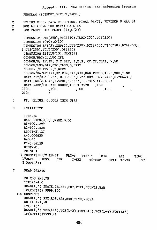
Appendix III. The Helium Data Reduction Program

PROGRAM HE(INPUT,OUTPUT,TAPE1)

C HELIUM COND. DATA REDUCTION, FINAL DR/DT, REVISED 9 MAR 81 C FOR LS ALONG THE DATA: CALL LS C FOR PLOT: CALL PLOT(G(1),G(2»

DIMENSION DTR(250),DTC(250),TLOG(250),VOF(250) DIMENSION F(40),G(10) DIMENSION BFY(5),GNU(S),DT1(250),DT2(250),DT3(250),DT4(250),

1 DT5(250),VOLT(250),QI(250) DIMENSION ITITLE(13),NAME(8) COMMON/DDC/LU,LUC,IFL COMMON/8/ IN,IK, P,T,DEN, E,R,S, CV,CP,CSAT, W,WK COMMON/LSS/DTR,DTC,TLOG,Q,PRTT COMMON /FITT/ F,Y,NFUN COMMON/DATATC/R1,R2,R3Z,R4Z,R3B,R4B,PRESS,TEMP,VOF,TINC DATA BFY/0.509927,-0.338935,O.271009,-0.232425,0.206431/ DATA GNU/2.4048,5.5201,8.6537,ll.7315,14.9309/ DATA NAME/10HHANS RODER,10H X 3528 ,lOR

110H ,10H ,lOR ,10H 210H /

CPT, HELIUM, 0.0005 INCH WIRE

C INITIALIZE

IFL=156 CALL GRPH(0,0,8,NAME,0,0) R1=100.1299 R2=100.1428 RHOPT=21.37 A=0.000635 B=0.45 PI=3.14159 DENT=20. PRINT 1

1 FORMAT(lR1/* RUNPT PRT-T WIRE-T R3Z R4Z TINC 1VOLTS PRESS DEN T-EXP TC-EXP STAT TC-TN PCT 2 POWER*/)

C READ DATATC

DO 200 K=1,78 TTRIAL=1.0 READ(l,*) IDATE,IRUNPT,PRT,PRT1,COUNTS BAR IF(EOF(l» 9999,100 '

100 CONTINUE READ(l,*) R3Z,R3B,R4Z,R4B,TINC,VNOVA DO 11 1=1,50 L=(I-1)*5 READ(l,*) VOF(L+1),VOF(L+2),VOF(L+3) VOF(L+4) VOF(L+5) IF(EOF(1»9999,11 "

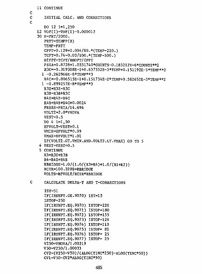
11 CONTINUE C C INITIAL CALC. AND CORRECTIONS C

DO 12 1=1,250 12 VOF(I)=VOF(1)-0.000012 30 R=PRT/2000.

PRTT=TEMPP(R) TEMP=PRTT CPPT=0.129+0.004/80.*(TEMP-220.) TCPT=0.74-0.03/100.*(TEMP-300.) DIFPT=TCPT/RHOPT/CPPT PS1A=0.8728+1.0351740*COUNTS-0.183212E-6*COUNTS**2 R3C=-O.319308E-l+0.637332E-3*TEMP+O.151192E-5*TEMP**2

1 -O.262966E-8*TEMP**3 R4C=-O.806515E-l+0.151734E-2*TEMP+0.582652E-5*TEMP**2

1 -O.899257E-8*TEMP**3 R3Z=R3Z-R3C R3B=R3B+R3C R4Z=R4Z-R4C R4B=R4B+R4C+O.0024 PRESS=PS1A/14.696 VOLT2=2.0*VNOVA VEST=O.5 DO 4 1=1,50 HPVOLT=VEST+O.1 VM1N=HPVOLT*O.99 VMAX=HPVOLT*1.01 1F(VOLT2.GT.VM1N.AND.VOLT2.LT.VMAX) GO TO 5

4 VEST=VEST+O.5 5 CONTINUE

R3=R3Z+R3B R4=R4Z+R4B RBR1DGE=1.0/(1.0/(R3+R4)+1.0/(R1+R2» RC1R=100.3288+RBRIDGE VOLTS=HPVOLT/RC1R*RBR1DGE

C CALCULATE DELTA-T AND T-CORRECTIONS

1ST=51 1F(IRUNPT.GE.9070) 1ST=15 ISTOP=250 IF(1RUNPT.EQ.9070) ISTOP=220 IF(1RUNPT.EQ.9071) ISTOP=180 1F(1RUNPT.EQ.9072) ISTOP=155 1F(IRUNPT.EQ.9073) ISTOP=126 1F(IRUNPT.EQ.9074) ISTOP=110 1F(IRUNPT.EQ.9075) 1STOP= 82 IF(1RUNPT.EQ.9076) ISTOP= 25 IF(1RUNPT.EQ.9077) ISTOP= 25 V250=VNOVA/1.00319 V50=V250/1.00033 CV2=(V250-V50)/(ALOG(T1NC*250)-ALOG(TINC*50» CV1=V50-CV2*ALOG(TINC*50)

485

DO 8 1=1,250 8 VOLT(1)=CV1+CV2*ALOG(T1NC*I)

DTW=(F1NDDT(VOLT(1ST),VOF(IST),TTRIAL)+FINDDT(VOLT(1STOP), 1 VOF(1STOP),TTR1AL»/2.

TEM=DTW+TEMP RESW3=F1ND1(TEM) RESW4=F1ND2(TEM) RTOTAL=R3B+R4B+RESW3+RESW4 1Q=(1ST+1STOP)/2+1 Q=(VOLT(1Q)/RTOTAL)**2*(RESW3+RESW4)*100./15.596 DEN=FNDDHE(PRESS,TEMP) RHOGAS=DEN*4.0026/1000. TC=THERHE(DEN,TEMP)/10. CPGAS=CPHE(DEN,TEMP)/4.0026 CVGAS=CVHE(DEN,TEMP) D1FGAS=TC/100./RHOGAS/CPGAS QQ=Q/(4.*P1*TC) QQQ=Q*8.3143*10./(DEN*CPGAS*39.948*CVGAS*P1*B**2) QQQQ=8.*P1*A/100.*5.6697E-8*TEMP**3/Q T1ME=O. DO 3 1=1,250 TlME=T1ME+T1NC TLOG(1)=ALOG(T1ME*1000.) DELT=QQ*ALOG(4.0*D1FGAS*T1ME/A**2/1.781) DTR(1)=F1NDDT(VOLT(1),VOF(1),TTR1AL) TTRIAL=DTR(I) DT1(1)=A**2*(RHOPT*CPPT-RHOGAS*CPGAS)/(2.*TC/I00.*T1ME)*DELT

1 -QQ*A**2/(4.*D1FGAS*T1ME)*(2.-D1FGAS/D1FPT) DT2(1)=0. BKT=B**2/(D1FGAS*T1ME) 1F(BKT.GT.5.78) GO TO 10 BRAK=O. DO 9 J=I,5

9 BRAK=BRAK+EXP(-GNU(J)**2*D1FGAS*T1ME/B**2)*(P1*BFY(J»**2 DT2(1)=QQ*(ALOG(4.0*D1FGAS*T1ME/B**2/1.781)+BRAK)

10 CONTINUE DT3(1)=-QQQ*T1ME DT4(1)=0. DT5(1)=QQQQ*DELT**2 DTC(I)=DTR(1)+DTl(1)+DT2(I)+DT3(1)+DT4(1)+DT5(1) TTT=TEMP+DTR(1) R3=F1ND1(TTT)+R3B R4=FIND2(TTT)+R4B RBRIDGE=I.0/(1.0/(R3+R4)+1.0/(R1+R2» VOLT(1)=HPVOLT*RBR1DGE/(RBRIDGE+I00.3288) RTOTAL=R3+R4 RESW3=R3-R3B RESW4=R4-R4B QI(I)=(VOLT(I)/RTOTAL)**2*(RESW3+RESW4)*100./15.596

3 CONTINUE DO 54 1=1,250

54 DTC(I)=DTC(I)*QI(1Q)/Q1(I)

C LEAST SQUARE DELTA-T VS. LOG(T1MES)

486

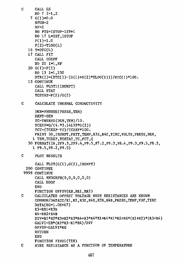
C CALL LS DO 7 1=1,2

7 G(I)=O.O NFUN=2 NF=2 NO PTS=ISTOP-IST+1 DO 17 L=IST,ISTOP F(1)=1.0 F(2)=TLOG(L)

16 Y=DTC(L) 17 CALL FIT

CALL COEFF DO 20 I=l,NF

20 G(I)=F(I) DO 13 1=1,250 DTR(I)=(DTC(I)-(G(1)+G(2)*TLOG(I»)/DTC(I)*100.

13 CONTINUE CALL PLOT1(IRUNPT) CALL STAT TCSTAT=F(2)/G(2)

C CALCULATE THERMAL CONDUCTIVITY

DEN=FNDDHE(PRESS,TEM) DENT=DEN TC=THERHE(DEN,TEM)/10. TCEXP=Q/(4.*3.14159*G(2» PCT=(TCEXP-TC)/TCEXP*lOO. PRINT SO,IRUNPT,PRTT,TEMP,R3Z,R4Z,TINC,VOLTS,PRESS,DEN,

1 TEM,TCEXP,TCSTAT,TC,PCT,Q 50 FORMAT(I6,2F9.3,2F9.4,F9.5,F7.2,F9.3,F8.4,F9.3,F9.S,F8.3,

1 F9.5,F8.2,F9.S)

C PLOT RESULTS

CALL PLOT(G(1),G(2),IRUNPT) 200 CONTINUE

9999 CONTINUE CALL ENDGRPH(O,O,O,O,O,O) CALL DDDF END FUNCTION OFFSV(EB,RR1,RR2)

C CALCULATES OFFSET VOLTAGE WHEN RESISTANCES ARE KNOWN COMMON/DATATC/Rl,R2,R3Z,R4Z,R3B,R4B,PRESS,TEMP,VOF,TINC DATA(RG=1.0E+07) R3=RR1+R3B R4=RR2+R4B DIV=R1*R2*R3+R2*R3*R4+R3*R4*Rl+R4*Rl*R2+RG*(Rl+R2)*(R3+R4) GALVI=EB*(R2*R3-R1*R4)/DIV OFFSV=GALVI*RG RETURN END FUNCTION FIND1(TtN)

C WIRE RESISTANCE AS A FUNCTION OF TEMPERATURE

487

COMMON/DATATC/Rl,R2,R3Z,R4Z,R3B,R4B,PRESS,TEMP,VOF,TINC P=PRESS*14.696 IF(TIN.GT.150.) GO TO 2 FINDl=-10.231206+O.3670809*TIN-0.9903371E-4*TIN**2-0.5375358E-5*P RETURN

2 FINDl=-9.0654718+0.35344447*TIN-0.59234427E-4*TIN**2-0.966271E-5*P RETURN END FUNCTION FIND2{TIN)

C WIRE RESISTANCE AS A FUNCTION OF TEMPERATURE COMMON/DATATC/Rl,R2,R3Z,R4Z,R3B,R4B,PRESS,TEMP,VOF,T1NC P=PRESS*14.696 IF(TIN.GT.150.) GO TO 2 FIND2=-5.057558+O.1823527*TIN-0.525728E-4*TIN**2-0.285743E-5*P RETURN

2 FIND2=-4.346459+0.17402506*TIN-0.2831553E-4*T1N**2-0.452695E-5*P RETURN E~

FUNCTION FINDDT{Vl,V2,Tl) C AN APPROXIMATION, TO REPLACE WIRE-R

COMMON/DATATC/Rl,R2,R3Z,R4Z,R3B,R4B,PRESS,TEMP,VOF,T1NC V=V2 TT=Tl+TEMP DO 10 1=1,10 REl=FINDl(TT) RE2=FIND2(TT) VOFFI =OFFSV(Vl,REl,RE2) IF(ABS(V-VOFFl)-1.0E-6 ) 20,20,1

1 T=TT+O.Ol REl=FINDl{T ) RE2=FIND2{T ) VOFF2 =OFFSV(Vl,REl,RE2) DVDT=(VOFF2-VOFFl)/0.01 CORR=(V-VOFFl)/DVDT

10 TT=TT+CORR 20 FINDDT=TT-TEMP

RETURN END FUNCTION TEMPP(R)

C ABBR. FOR 1776265 FROM 70 TO 310 K, CORR.12/19/80 DIMENSION RR(241) DATA(RR(I),I=I,131)/3.99645, 4.10575, 4.21531, 4.32508, 4.43505,

1 4.54520, 4.65550, 4.76594, 4.87649, 4.98714, 5.09788, 5.20868, 2 5.31954, 5.43045, 5.54139, 5.65235, 5.76332, 5.87430, 5.98527, 3 6.09622, 6.20716,6.31807,6.42895,6.53979,6.65058, 4 6.76134,6.87204,6.98268,7.09327,7.20379, 5 7.31426,7.42465,7.53498,7.64523,7.75541, A 7.86552,7.97555,8.08550,8.19538, 8.30517,8.41489,8.52453, B 8.63408, 8.74356, 8.85295, 8.96226, 9.07149, 9.18065, 9.28971, C 9.39870, 9.50761, 9.61644, 9.72519, 9.83386, 9.94245,10.05096, D 10.15939,10.26775,10.37603,10.48424,10.5923/,10.70043,10.80841, E 10.91632,11.02416,11.13192,11.23962,11.34725,11.45480,11.56229, F 11.66971,11.77707,11.88435,11.99158,12.09873,12.20583,12.31286, G 12.41982,12.52673,12.63357,12.74036,12.84708,12.95375,13.06036,

~8

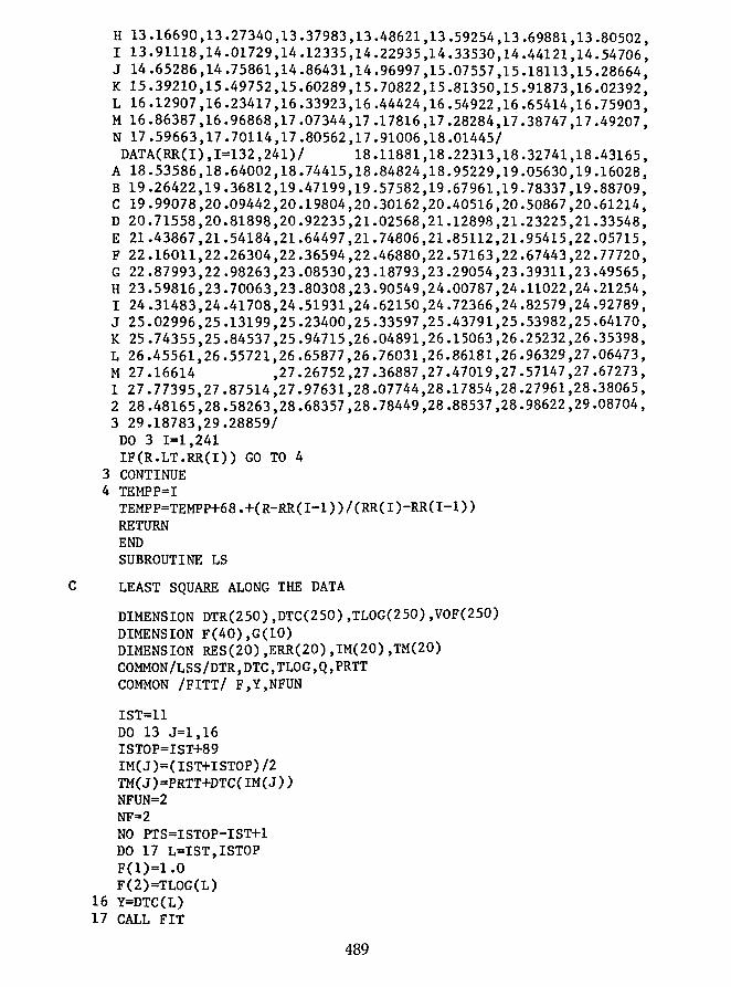
H 13.16690,13.27340,13.37983,13.48621,13.59254,13.69881,13.80502, I 13.91118,14.01729,14.12335,14.22935,14.33530,14.44121,14.54706, J 14.65286,14.75861,14.86431,14.96997,15.07557,15.18113,15.28664, K 15.39210,15.49752,15.60289,15.70822,15.81350,15.91873,16.02392, L 16.12907,16.23417,16.33923,16.44424,16.54922,16.65414,16.75903, M 16.86387,16.96868,17.07344,17.17816,17.28284,17.38747,17.49207, N 17.59663,17.70114,17.80562,17.91006,18.01445/ DATA(RR(I),I=132,241)/ 18.11881,18.22313,18.32741,18.43165,

A 18.53586,18.64002,18.74415,18.84824,18.95229,19.05630,19.16028, B 19.26422,19.36812,19.47199,19.57582,19.67961,19.78337,19.88709, C 19.99078,20.09442,20.19804,20.30162,20.40516,20.50867,20.61214, D 20.71558,20.81898,20.92235,21.02568,21.12898,21.23225,21.33548, E 21.43867,21.54184,21.64497,21.74806,21.85112,21.95415,22.05715, F 22.16011,22.26304,22.36594,22.46880,22.57163,22.67443,22.77720, G 22.87993,22.98263,23.08530,23.18793,23.29054,23.39311,23.49565, H 23.59816,23.70063,23.80308,23.90549,24.00787,24.11022,24.21254, I 24.31483,24.41708,24.51931,24.62150,24.72366,24.82579,24.92789, J 25.02996,25.13199,25.23400,25.33597,25.43791,25.53982,25.64170, K 25.74355,25.84537,25.94715,26.04891,26.15063,26.25232,26.35398, L 26.45561,26.55721,26.65877,26.76031,26.86181,26.96329,27.06473, M 27.16614 ,27.26752,27.36887,27.47019,27.57147,27.67273, 1 27.77395,27.87514,27.97631,28.07744,28.17854,28.27961,28.38065, 2 28.48165,28.58263,28.68357,28.78449,28.88537,28.98622,29.08704, 3 29.18783,29.28859/

DO 3 1=1,241 IF(R.LT.RR(I» GO TO 4

3 CONTINUE 4 TEMPP=I

TEMPP=TEMPP+68.+(R-RR(I-1»/(RR(I)-RR(I-1» RETURN

SUBROUTINE LS

C LEAST SQUARE ALONG THE DATA

DIMENSION DTR(250),DTC(250),TLOG(250),VOF(250) DIMENSION F(40),G(10) DIMENSION RES(20),ERR(20),IM(20),TM(20) COMMON/LSS/DTR,DTC,TLOG,Q,PRTT COMMON /FITT/ F,Y,NFUN

IST=11 DO 13 J=1,16 ISTOP=IST+89 IM(J)=(IST+ISTOP)/2 TM(J)=PRTT+DTC(IM(J» NFUN=2 NF=2 NO PTS=ISTOP-IST+1 DO 17 L=IST,ISTOP F(1)=1.0 F(2)=TLOG(L)

16 Y=DTC(L) 17 CALL FIT

489

CALL COEFF RES(J)=Q/(4.*3.l4l59*F(2» CALL STAT ERR(J)=RES(J)/(Q/(4.*3.14159*F(2»)

13 IST=IST+lO PRINT l5,«IM(J),TM(J»,J=1,lO) PRINT l4,«RES(J),ERR(J»,J=1,lO) PRINT l5,«IM(J),TM(J»,J=11,16) PRINT l4,«RES(J),ERR(J»,J=11,16)

14 FORMAT(5X,20F6.4) 15 FORMAT(5X,lO(I4,F8.3»

RETURN END SUBROUTINE PLOT(Gl,G2,IDNO)

C PLOTS RESULTS DIMENSION ITITLE(13),NAME(8),ICOMM(2) DIMENSION DTR(250),DTC(250),TLOG(250),VOF(250) COMMON/LSS/DTR,DTC,TLOG,Q,PRTT DATA ITITLE/lOH ,10H HELIUM T,lOHHERMAL CON,

110HDUCTIVITY ,10H ,10H ,10HLN(T) TIN, 2l0H MILLISEC ,10H ,10H ,10HDELTA T, 3l0HT IN K ,10H /

DATA ICOMM(l)/lOH RUNPT / ENCODE(lO,1,ICOMM(2»IDNO

1 FORMAT(IlO) NO PTS=240 DO 51 1=11,250 L=I-lO TLOG(L)=TLOG(I)

51 DTC(L)=DTC(I) CALL PGRPH(TLOG,DTC,NO PTS,ITITLE,0,6) DTC(1)=Gl+G2*TLOG(1) DTC(2)=Gl+G2*TLOG(NO PTS) TLOG(2)=TLOG(NO PTS) CALL CLGRPH(TLOG,DTC,2,0,0,0) ABFRACT=0.05 ORDFR=0.9 CALL COMGRPH(ABFRACT,ORDFR,2,ICOMM) RETURN END SUBROUTINE PLOTl(IDNO)

C PLOTS DEV. FROM LS LINES DIMENSION ITITLE(13),NAME(8),TT(250),ICOMM(2) DIMENSION DTR(250),DTC(250),TLOG(250),VOF(250) COMMON/LSS/DTR,DTC,TLOG,Q,PRTT DATA ITITLE/lOH ,10H HELIUM T,lOHHERMAL CON,

110HDUCTIVITY ,10H ,10H ,10HLN(T), T I, 2l0HN MILLISEC,lOH ,10H ,10HDEV. FROM, 3l0HLS FIT ,10H /

DATA ICOMM(l)/lOH RUNPT / ENCODE(lO,1,ICOMM(2»IDNO

1 FORMAT(IlO) NO PTS=240 DO 51 1=11,250

490

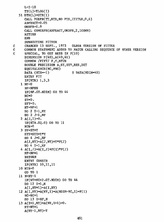
L=I-10 TT(L)=TLOG(I)

51 DTR(L)=DTR(I) CALL PGRPH(TT,DTR,NO PTS,ITITLE,0,6) ABFRACT=O.OS ORDFR=0.9 CALL COMGRPH(ABFRACT,ORDFR,2,ICOMM) RETURN END SUBROUTINE FITTER

C CHANGED 13 SEPT., 1973 OLDER VERSION OF FITTER C COMMON STATEMENT ADDED TO MATCH CALLING SEQUENCE OF NEWER VERSION C SPECIAL, TO GET RESS IN F(10)

DIMENSION F(40),A(40,41) COMMON IFITTI F,Y,NFUN DOUBLE PRECISION A,SY,SYY,RES,DET EQUIVALENCE(NC,FNC) DATA (NTR=-l) $ DATA(NDIM=40) ENTRY FIT IF(NTR) 1,3,3

1 NP=O NF=NFUN IF(NF.GT.NDIM) GO TO 44 NC=O SY=O. SYY=O. NY=NF+l DO 2 I=l,NY DO 2 J=l,NF

2 A(J,I)=O. IF(NTR.EQ.O) GO TO 11 NTR=O

3 SY=SY+Y SYY=SYY+Y*Y DO 4 J=l,NF A(J,NY)=A(J,NY)+Y*F(J) DO 4 I=l,NF

4 A(I,J)=A(I,J)+F(I)*F(J) NP=NP+1 RETURN ENTRY CONSTR IF(NTR) 10,11,11

10 NTR=O GO TO 1

11 N=NY-1 IF(NY+NC+2.GT.NDIM) GO TO 44 DO 12 I=l,N A(I,NY+1)=A(I,NY)

12 A(I,NY)=A(NY,I)=A(NDIM-NC,I)=F(I) NC=NC+1 DO 13 I=NF,N

13 A(I+l,NY)=A(NY,I+l)=O. NY=NY+1 A(NY-l,NY)=Y

491

RET~N

ENTRY COEFF N=NY-1 DO 20 I=1,NF

20 F(I)=A(I,NY) IF(N.EQ.1)GO TO 23 DO 22 I=2,N DO 21 J=I,NY

21 A(I-1,J)=A(I-1,J)/A(I-1,I-1) DO 22 J=I,N DO 22 K=I,NY

22 A(J,K)=A(J,K)-A(J,I-1)*A(I-1,K) 23 A(N,NY)=A(N,NY)/A(N,N)

IF(N.EQ.1)GO TO 26 DO 24 I=2,N L=N-I+2 DO 24 J=L,N

24 A(L-1,NY)=A(L-1,NY)-A(L-1,J)*A(J,NY) 26 NTR=-1

RES=SYY DO 25 I=1,NF RES=RES-F(I)*A(I,NY)

25 F(I)=A(I,NY) NFUN=NP DF=NP-NF+NC Y=FNC FNP=NP RETUllN ENTRY STAT IF(NC.LE.O)GO TO 28 DO 27 I=1,NC DO 27 J=1,NF

27 RES=RES-A(NDIM-I+1,J)*A(J,NY)*A(NF+I,NY) 28 TOT=SYY-SY*SY/FNP

REG=TOT-RES SYY=RES/DF ST=1.96+2.72/DF+8.04/DF**3 DET=1.0D+0 DO 30 I=1,NF DET=DET*A(I,I)

30 A(I,I)=1.0D+0/A(I,I) IF(NF.EQ.1)GO TO 322 DO 32 I=2,NF DO 32 J=2,I SY=O. DO 31 K=J,I

31 SY=SY-A(I,K-1)*A(K-1,J-1) 32 A(I,J-1)=SY*A(I,I)

322 CONTINUE DO 36 I=1,NF L=NF-I DO 33 J=1,L K=NF-J DO 33 M=1,J

492

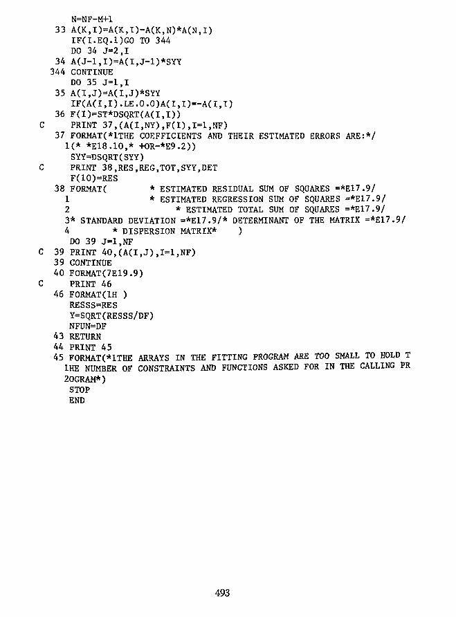
N=NF-M+l 33 A(K,I)=A(K,I)-A(K,N)*A(N,I)

IF(I.EQ.l)GO TO 344 DO 34 J=2,I

34 A(J-l,I)=A(I,J-l)*SYY 344 CONTINUE

DO 35 J=1,I 35 A(I,J)=A(I,J)*SYY

IF(A(I,I).LE.O.O)A(I,I)=-A(I,I) 36 F(I)=ST*DSQRT(A(I,I»

C PRINT 37,(A(I,NY),F(I),I=1,NF) 37 FORMAT(*1THE COEFFICIENTS AND THEIR ESTIMATED ERRORS ARE:*/

1(* *E18.10,* +OR-*E9.2» SYY=DSQRT(SYY)

C PRINT 38,RES,REG,TOT,SYY,DET F(10)=RES

38 FORMAT( * ESTIMATED RESIDUAL SUM OF SQUARES =*E17.9/ I * ESTIMATED REGRESSION SUM OF SQUARES =*E17.9/ 2 * ESTIMATED TOTAL SUM OF SQUARES =*EI7.9/ 3* STANDARD DEVIATION =*E17.9/* DETERMINANT OF THE MATRIX =*EI7.9/ 4 * DISPERSION MATRIX* )

DO 39 J=1,NF C 39 PRINT 40,(A(I,J),I=1,NF)

39 CONTINUE 40 FORMAT(7E19.9)

C PRINT 46 46 FORMAT(IH )

RESSS=RES Y=SQRT(RESSS/DF) NFUN=DF

43 RETURN 44 PRINT 45 45 FORMAT(*ITHE ~~YS IN THE FITTING PROGRAM ARE TOO SMALL TO HOLD T

IRE NUMBER OF CONSTRAINTS AND FUNCTIONS ASKED FOR IN THE CALLING PR 20GRAM*)

STOP END

493