A Tracer Test to Estimate Hydraulic Conductivities and ... Tracer Test to Estimate Hydraulic...
54
U.S. Department of the Interior U.S. Geological Survey A Tracer Test to Estimate Hydraulic Conductivities and Dispersivities of Sediments in the Shallow Aquifer at the East Gate Disposal Yard, Fort Lewis, Washington Water-Resources Investigations Report 99-4244 Prepared in cooperation with Department of the Army Fort Lewis Public Works Environmental and Natural Resources Division science fora changing world
Transcript of A Tracer Test to Estimate Hydraulic Conductivities and ... Tracer Test to Estimate Hydraulic...

U.S. Department of the Interior U.S. Geological Survey
A Tracer Test to Estimate Hydraulic Conductivities and Dispersivities of Sediments in the Shallow Aquifer at the East Gate Disposal Yard, Fort Lewis, Washington
Water-Resources Investigations Report 99-4244
Prepared in cooperation withDepartment of the ArmyFort Lewis Public WorksEnvironmental and Natural Resources Division
science fora changing world

A Tracer Test to Estimate Hydraulic Conductivities and Dispersivities of Sediments in the Shallow Aquifer at the East Gate Disposal Yard, Fort Lewis, Washington
By E.A. Prych
U.S. GEOLOGICAL SURVEY
Water-Resources Investigations Report 99-4244
Prepared in cooperation with
Department of the Army Fort Lewis Public Works Environmental and Natural Resources Division
Tacoma, Washington 1999

U.S. DEPARTMENT OF THE INTERIOR
BRUCE BABBITT, Secretary
U.S. GEOLOGICAL SURVEY
Charles G. Groat, Director
Any use of trade, product, or firm names in this publication is for descriptive purposes only and does not imply endorsement by the U.S. Government.
For additional information write to:
District ChiefU.S. Geological Survey1201 Pacific Avenue - Suite 600Tacoma, Washington 98402
Copies of this report can be purchased from:
U.S. Geological Survey Information Services Building 810Box 25286, Federal Center Denver, CO 80225-0286

CONTENTS
Abstract..............................................................^ 1Introduction .....................................................................................................................................^ 2
Purpose, method, and scope ........................................................................................................................................ 2Acknowledgment...................................................................................................^ 4Description of study area............................................................................................................................................. 4
Physical setting.................................................................................................................................................. 4Geohydrology.................................................................................................................................................... 4
The East Gate pump-and-treat system......................................................................................................................... 5Methods ...............................................................................................................................................................^ 6
Injection of tracers....................................................................................................................................................... 6Monitoring...........................................................................................................................................................^ 6Analysis of specific electrical conductance data......................................................................................................... 11
Hydraulic conductivity ...................................................................................................................................... 21Longitudinal dispersivity................................................................................................................................... 22
Ground-water flow directions................................................................................................................................................ 23Ground-water levels and flow directions..................................................................................................................... 23Bromide and chloride concentrations.......................................................................................................................... 27Specific electrical conductance.................................................................................................................................... 27
Estimated hydraulic conductivities and dispersivities........................................................................................................... 29Horizontal hydraulic conductivity............................................................................................................................... 29Vertical hydraulic conductivity.................................................................................................................................... 29Horizontal and vertical longitudinal dispersivities...................................................................................................... 29Discussion and applicability of estimates.................................................................................................................... 30
Summary and conclusions..................................................................................................................................................... 31References cited......................................................................._ 32Appendix A. Supplemental information............................................................................................................................... 33
FIGURES
1-2. Maps showing':1. Location of the East Gate Disposal Yard near the Logistics Center at Fort Lewis, Washington, and
the plume of dissolved trichloroethylene (TCE) in ground water...................................................................... 32. Schematic diagram of East Gate pump-and-treat system and nearby observation wells,
Fort Lewis, Washington ..................................................................................................................................... 53. Schematic diagram of East Gate pump-and-treat and tracer-test systems, Fort Lewis, Washington.......................... 74. Map showing locations of wells in tracer-test and pump-and-treat recharge area at East Gate
Disposal Yard, Fort Lewis, Washington, with observed ground-water levels, and inferred ground-waterflow directions and estimated velocities ..................................................................................................................... 8
5. Graphs showing specific electrical conductances and bromide and chloride concentrations in wellsas functions of time..................................................................................................................................................... 14
6-7. Diagrams showing:6. Section along a line through wells C25 and TRP-2 showing elevations of well screens, observed
water levels, and inferred ground-water flow directions and estimated velocities, Fort Lewis, Washington......................................................................................................................................................... 24
7. Section along a line through wells LR-1 and LR-2 showing elevations of well screens, observed water levels, and inferred ground-water flow directions and estimated velocities, Fort Lewis, Washington......................................................................................................................................................^ 25
Al. Graph showing excess specific electrical conductance as a function of bromide concentration in samples.............. 48

TABLES
1. Characteristics and observed water levels in wells................................................................................................. 92. Concentrations of bromide and chloride, and specific-conductances of water samples......................................... 123. Computed centroids and standard deviations of temporal distributions of observed vertically averaged
values of specific electrical conductance in excess of ambient values................................................................... 204. Estimated values of hydraulic conductivities and longitudinal dispersivities, and data used to compute
them .....................................................................................................................................................,......^ 26Al. Summary of specific electrical conductance and temperature data........................................................................ 34
CONVERSION FACTORS AND VERTICAL DATUM
Multiply By To Obtain
acre 0.4047 hectareinch (in) 25.4 millimeterfoot (ft) 0.3048 metergallon (gal) 3.785 litermile (mi) 1.609 kilometer
Temperature: To convert temperature given in this report in degrees Celsius (°C) to degrees Fahrenheit (°F)/ use the following equation: °F = 9/5°C+32.
Sea Level: In this report "sea level" refers to the National Geodetic Vertical Datum of 1929 (NGVD of 1929) a geodetic datum derived from a general adjustment of the first-order level nets of both the United States and Canada, formerly called Sea Level Datum of 1929.
IV

A Tracer Test to Estimate Hydraulic Conductivities and Dispersivities of Sediments in the Shallow Aquifer at the East Gate Disposal Yard, Fort Lewis, Washington
By E.A. Prych
ABSTRACT
Knowledge of the hydraulic characteristics of the unconsolidated glacial sediments that make up the shallow aquifer at Fort Lewis, a U.S. Army facility in western Washington, is necessary for use in the numerical models of ground-water flow and solute transport that are being used by the U.S. Geological Survey and others to design and evaluate alternatives for the remediation of subsurface contamination at and downgradient of the East Gate Disposal Yard near the Logistics Center at the fort. Data from a tracer test, which utilized an existing pump-and-treat system at the disposal yard, were used to estimate hydraulic conductivities and longitudinal dispersivi- ties in horizontal and vertical directions. During the tests, the outflow from the pump-and-treat plant was dosed with potassium bromide before being returned to the ground-water system through two 100-foot- long horizontal recharge galleries and a 110-foot- deep recharge well. Specific electrical conductance was monitored in 16 observations wells, and a few samples were collected from most of the wells for determining bromide concentrations.
The water table at the test site was less than 10 feet (ft) below land surface, and ground-water- flow directions, as inferred from water levels, were generally northwesterly, but flow patterns were com plex. This complexity, which probably is caused in part by the heterogeneity of the sediments, is reason for those working to remediate contamination at the Logistics Center to be cautious when planning reme diation and when drawing conclusions from observed distributions of contaminant concentrations.
Differences between water levels and between centroids and variances of the temporal distributions of excess (observed minus ambient) specific conduc
tance at pairs of locations were used to estimate hydraulic conductivities and longitudinal dispersivi- ties. Although the equations used for estimating hydraulic conductivities and dispersivities are based on assumptions of rectilinear or radial flow, which were assumed to be reasonable at the scale of dis tances between observation locations, deviations from these idealized flows and other assumptions can introduce errors of unknown magnitude; therefore, the estimated values should be used with caution.
Analyses of data from five pairs of horizon tally separated locations near the water table yielded estimates of horizontal hydraulic conductivity between 69 and 3,100 feet per day (ft/d), and esti mates of horizontal longitudinal dispersivity that ranged from 6.9 to 28 ft. Data from a pair of wells screens at about 80 ft below land surface yielded val ues of horizontal hydraulic conductivity between 2,300 and 3,800 ft/d. The largest estimated values of horizontal hydraulic conductivity are larger than those obtained for the East-Gate area by earlier inves tigators from calibration of a ground-water flow model (80 to 260 ft/d) and from aquifer tests (16 to 330 ft/d), probably because the values from the tracer test are biased toward thin (probably less than 10 ft) highly permeable units of the aquifer, while the val ues from the earlier studies are averages over a large fraction or entire thickness of the approximately 100- foot-thick aquifer. Analyses of data from four pairs of vertically separated locations yielded vertical hydrau lic conductivities between 8 and 590 ft/d and vertical longitudinal dispersivities that ranged from 1.8 to 12 ft for the upper 40 ft of sediments below land sur face.

INTRODUCTION
From about 1946 to 1971 the U.S. Army dumped or buried waste trichloroethylene (TCE) and other materials in the East Gate Disposal Yard near the Logistics Center on Fort Lewis, Washington (Woodward Clyde, 1998). As a result, a plume of TCE- contaminated ground water in the shallow water-table aquifer (about 100 ft thick) now extends from the disposal yard, beneath the Logistics Center, to near American Lake and the community of Tillicum, which are located about 2 miles (mi) northwest of the disposal yard (fig. 1). In 1995 two pump-and-treat systems, one near and downgradient of the East Gate Disposal Yard and another near U.S. Interstate 5 and upgradient of the boundary between Fort Lewis and Tillicum, were installed in the shallow aquifer to intercept the transport of contaminants by ground water out of the disposal yard and from Fort Lewis to neighboring areas, respectively. In addition to concerns about the plume in the shallow aquifer, there are also concerns about the movement of contaminants from the shallow to a deeper aquifer.
Cantrell and others (1998) estimated that if no other remediation work is done at the site, it may be necessary to operate the pump-and-treat systems for 76 to 160 years or more to clean up the ground-water system. Consequently, the Army is investigating methods to accelerate the removal of TCE and other volatile organic compounds (VOC's) from the subsurface and the attenuation of VOC concentrations in ground water. The design and evaluation of many of the methods use numerical models of ground-water flow and transport, which in turn require knowledge of the hydraulic conductivities and dispersivities of the subsurface materials. An existing three-layer model that was developed and used by the U.S. Army Corps of Engineers (1998) and that was modified by H. H. Bauer of the U.S. Geological Survey (Sue C. Kahle, U. S. Geological Survey, written commun., October 5,1998) simulates the entire shallow aquifer as a single layer. The model uses hydraulic conductivities of the upper layer that were obtained (1) by analyses of traditional aquifer tests in which changes in ground- water levels are observed after the start or cessation of pumping from a well and (2) by calibrating the numerical model so that model-simulated water levels agree with those observed. Because transport probably is not uniform over the depth of this aquifer as a result of preferred movement within layers of coarse-grained sediments with relatively high permeability and as a
result of a nonuniform vertical distribution of the contaminant source, the existing modified model is being further modified by subdividing the model layer that represents the upper aquifer into multiple layers of different hydraulic characteristics. Knowledge of the hydraulic characteristics of the individual layers within the upper aquifer is necessary for making this modification as well as for assisting in the interpretation of observed distributions of contaminant concentrations and for the designing remediation systems.
Purpose, Method, and Scope
This report describes and presents the results of a tracer test performed in and near the East Gate Disposal Yard and pump-and-treat system to estimate hydraulic conductivities and dispersivities of parts of the shallow (less than 100 ft) subsurface sediments. As part of the test, the outflow from the treatment plant was dosed continuously over a 3-day period with a tracer, potassium bromide (KBr), before the treated water was reinjected into the ground though two recharge galleries and a recharge well. In addition, the water discharged into the well was dosed with sodium chloride (NaCl). Before, during, and for about 6 weeks after the addition of the tracers, in-situ specific electrical conductance of the water (referred to in the remainder of this report as specific conductance or conductance) in 16 wells was monitored, and a few water samples were collected from most of these wells for determinations of specific conductance, and bromide and chloride concentrations. Differences between water levels, between centroids (average arrival times), and between variances (spreading) of the temporal distributions of specific conductance above ambient levels at selected pairs of locations were used to infer local ground-water flow directions and to estimate hydraulic conductivities and longitudinal dispersivities in the horizontal and vertical directions. Because most of the horizontal tracer movement probably was within layers with high values of permeability, the estimates of horizontal hydraulic conductivity and dispersivity probably were biased toward these layers.

WA
SH
ING
TO
N
East
Gate
D
isp
osa
l Y
ard
^
Tre
atm
en
t
Rai
nier
Driv
eT
ilhcu
mF
ort
Le
wis
L
og
istic
s C
en
ter
Loca
tion
flno
Tre
atm
en
t p
lan
t
../
Z _ EX
PL
AN
AT
ION
Ma
dig
an
Hosp
ital 3
r^ '
10
0
C
once
ntra
tion
of T
CE
in
mic
rogr
ams
per
liter
.
o Lo
catio
n of
wel
l
10
00
2
00
0
30
00
4
00
0
50
00
FE
ET
1200
15
00 M
ET
ER
S
Figu
re 1
. Lo
catio
n of
the
Eas
t G
ate
Dis
posa
l Yar
d ne
ar th
e Lo
gist
ics
Cen
ter
of F
ort
Lew
is,
Was
hing
ton,
and
the
plum
e of
dis
solv
ed t
richl
oroe
thyl
ene
(TC
E)
in g
roun
d w
ater
(TC
E is
ocon
cent
ratio
ns fr
om W
oodw
ard-
Cly
de,
1997
).

Acknowledgment
The work described in this report was part of a larger study funded by the Department of the Army through Military Inter-departmental Purchase Request 8EUSGS4012, which was administered by Mr. Dennis Korycinski, Installation Restoration Program Manager, Fort Lewis Public Works, Environmental and Natural Resources Division.
Description Of The Area
Fort Lewis is located in the Puget Sound lowlands of western Washington about 10 mi southwest of the city of Tacoma. The East Gate Disposal Yard occupies about 13 acres near the southeast end of the Logistics Center, which in turn is located near the northeast corner of Fort Lewis (fig. 1).
Physical Setting
The Logistics Center sits on a gently rolling uplands plain about 280 ft above sea level. This plain is underlain by over 1,000 ft of unconsolidated glacial and inter-glacial sediments (Jones, 1996). The area where the tracer test was conducted is vegetated mostly with Douglas fir, black cottonwood, red alder and wild cherry trees, Scotch broom and other hardwood shrubs, and grasses. The roads in the area of the tracer test and in the East Gate Disposal Yard are unpaved, and there are no streams; however, most roads and many industrial and parking areas elsewhere in the Logistics Center are paved, and nearby Murray Creek flows through marshy areas south and west of the Logistics Center (fig. 1). Mean annual precipitation at Fort Lewis is about 40 inches per year (in/yr), and evapotrans- piration is about half of that. Precipitation in Tacoma during March 1998, when a large part of the test was conducted, was 4.52 inches (National Oceanic and Atmospheric Administration, 1998).
Geohydrology
The upper 100 ft or so of sediments, where nearly all the data were gathered during the tracer test and where most of the TCE plume is located, is commonly referred to as the upper aquifer (Shannon & Wilson, 1986). It consists of a widespread deposit of glacial outwash gravels about 20 ft thick near the surface that is underlain by a complex distribution of layers and lenses of till, glacial outwash sands and
gravels, and scattered deposits of non-glacial sediments near the bottom. In most places, a confining layer of mostly fine-grained material (silts and clays, primarily of interglacial origin) underlies the upper aquifer and separates it from a lower aquifer that consists mostly of older glacial sediments.
In the area of the tracer test the water table is less than about 10 ft below land surface, and parts of the surficial outwash gravels are saturated. The general direction of ground-water flow in the upper aquifer, as inferred from a water-level contour map (U.S. Army Corps of Engineers, 1998, fig. 5) and the TCE plume (fig. 1), is from the southeast to the northwest (from the East Gate Disposal Yard to American Lake); however, the complex distribution of fine- and coarse-grained layers and lenses within the upper aquifer may cause local ground-water flow patterns to be complex. Lithologic logs from wells less than 100 ft apart can be quite different, suggesting that there can be a large amount of uncertainty in the spacial geometry of individual units as inferred from lithologic information from wells (see, for example, U.S. Army Corps of Engineers, 1993, figs. 1-4 to 1-9).
Horizontal hydraulic conductivities of the sediments in the upper aquifer obtained by model calibration ranged from 80 to 260 ft/d in the East Gate area and from 40 to 380 ft/d in the entire Logistics Center (Michael M. Easterly, U.S. Army Corps of Engineers, Seattle, Wash., written commun., September 19, 1997). Values obtained from aquifer tests during which water was pumped from extraction or recharge wells of the East Gate pump-and-treat system (see the following section for a description of this system) range from 16 to 330 ft/d, and the ratio of horizontal to vertical hydraulic conductivity ranged from 12 to 259 (U.S. Army Corps of Engineers, 1993, tables 4-2 and 4-4). The horizontal hydraulic conductivities in the numerical model are vertical averages over the approximately 100-ft thickness of the upper aquifer and horizontal averages over areas with horizontal dimensions of several model cells (one to several hundreds of feet), while horizontal hydraulic conductivies from the aquifer tests probably approximate vertical averages over intervals equal to or larger than the thicknesses of the screened intervals of the pumped wells (from 10 to 30 ft) and horizontal averages over the area of influence of the pumped well (radii up to a few hundred feet).
The East Gate Pump-and Treat System
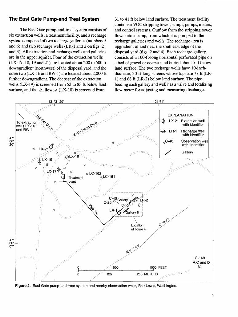
The East Gate pump-and-treat system consists of six extraction wells, a treatment facility, and a recharge system composed of two recharge galleries (numbers 5 and 6) and two recharge wells (LR-1 and 2 on figs. 2 and 3). All extraction and recharge wells and galleries are in the upper aquifer. Four of the extraction wells (LX-17,18,19 and 21) are located about 200 to 500 ft downgradient (northwest) of the disposal yard, and the other two (LX-16 and RW-1) are located about 2,000 ft farther downgradient. The deepest of the extraction wells (LX-19) is screened from 53 to 83 ft below land surface, and the shallowest (LX-18) is screened from
31 to 41 ft below land surface. The treatment facility contains a VOC stripping tower, sumps, pumps, meters, and control systems. Outflow from the stripping tower flows into a sump, from which it is pumped to the recharge galleries and wells. The recharge area is upgradient of and near the southeast edge of the disposal yard (figs. 2 and 4). Each recharge gallery consists of a 100-ft-long horizontal perforated pipe on a bed of gravel or coarse sand buried about 5 ft below land surface. The two recharge wells have 10-inch- diameter, 30-ft-long screens whose tops are 78 ft (LR- 1) and 68 ft (LR-2) below land surface. The pipe feeding each gallery and well has a valve and totalizing flow meter for adjusting and measuring discharge.
121°31'20"
To extraction wells LX-16 and RW-1
sPvP
47° 06' 20"
<5> LX-21,^
LX-19
J!6 //
I LX-17
o
^
o ->- jLX-18
Q ""-,::>
EXPLANATION
LX-21 Extraction well with identifier0
-e- LR-I
C-40
/
Recharge well with identifier
Observation well with identifier
Gallery
o
oLC-162 Treatment Q/LC-161 plant
47° 06' 07"
LC-149 A,C and D
Figure 2. East Gate pump-and-treat system and nearby observation wells, Fort Lewis, Washington.

METHODS
The tracer test was conducted in the vicinity of the recharge area of the East Gate pump-and-treat system and utilized the recharge galleries and one of the two recharge wells to introduce tracers into the ground water. During the test, the metered discharges into galleries 5 and 6 were 270 and 330 gallons per minute (gpm), respectively, and the metered discharge into well LR-1 was 180 gpm. No water was being discharged into well LR-2 during the test. Although none of the flow meters were calibrated as part of this study, the sum of the metered discharges into the two galleries and one recharge well equals 780 gpm, which is nearly the same as the metered discharge through the treatment plant, 790 gpm.
Injection of Tracers
About 530 gallons of a KBr solution at about 80 percent saturation was prepared in a trailer-mounted plastic tank and pumped into the outflow pipe of the stripping tower (fig. 3) for 3 days at a rate of 0.12 gpm. Dosing with KBr started at 10:20 a.m. on March 3, 1998, and ended at 10:20 a.m. on March 6. The dosing rate of the solution was monitored with a flow meter and was checked volumetrically a few times per day. Dosing with the KBr solution increased the specific conductance of the water from about 125 micro Siemens per centimeter (uS/cm) to about 200 uS/cm, and increased the bromide concentration from less than 0.05 milligrams per liter (mg/L) to about 40 mg/L.
In addition to the KBr solution, about 200 gallons of NaCl solution at about 70 percent saturation was prepared in another plastic tank on the bed of a truck and was fed by gravity into recharge well LR-01. The purpose of the NaCl tracer was to enable distinguishing between KBr tracer that entered the ground water through the shallow galleries and that which entered through the recharge well. The dosing rate of the NaCl solution was controlled with a valve, monitored with a flow meter, and checked volumetrically. In the experimental design the NaCl solution was to be added over the same time period as the KBr; however, repeated formation of gas bubbles in the NaCl feed line resulted in a sporadic and lower- than-planned dosing rate during most of the 3 days that KBr was added. The bubbles stopped appearing near the end of the 3-day period, and the NaCl was added to
the well for two additional days (without the addition of KBr at the treatment plant) until 10:30 a.m. on March 8 at a rate of about 0.036 gpm. Although it was not possible to measure the specific conductance or chloride concentration in the water after dosing with NaCl, the calculated approximate increase in chloride concentration was from about 2.5 mg/L to 30 mg/L when dosing at the desired rate; and the approximate increase in specific conductance was from about 200 uS/cm to 290 uS/cm or from 125 uS/cm to 215 uS/ cm, depending on whether or not the outflow from the treatment plant was being dosed with KBr.
Monitoring
The movement of tracers through the ground- water system was monitored by two methods. One by routinely measuring in-situ vertical profiles of specific electrical conductance within the screened intervals of 16 observation wells (including the inactive recharge well, LR-2) at a frequency that varied from a few times per day at the beginning of the test to once every few days at the end of the test for a period of about 6 weeks, and the other by occasionally pumping samples from the wells during this period and analyzing the samples for specific conductance, and for bromide and chloride concentrations. The observation wells were located within about 50 to 700 ft of the recharge galleries and recharge well (fig. 4). The screened intervals of the wells varied from 5 to 15 ft below land surface (well A15) to 139 to 149 ft (well LC-26D), but most were less than 50 ft deep (table 1). Six of the wells (A15, A30, A45, B15, C25, and C40; numbers in these identifiers are approximate well depths in feet below land surface) were installed for this test using an auger; the others already existed. The casings and screens of most wells were either 2 or 4 inches in diameter (table 1).
Specific conductance of the treated water before and after dosing with KBr (effluent of the stripping tower, and inflow to recharge well LR-1 before dosing with NaCl, respectively) was also monitored. Water temperatures always were measured along with specific conductance. Water levels in the wells were measured twice during the test. Data on the ambient values of specific conductance, and bromide and chloride concentrations were collected about 1 week before the start of the test (February 25,26, and 27) and a few hours before the test (March 3).

Trea
tmen
t
plan
t
Ext
ract
ion
wel
ls
LX-1
7, 1
8, 1
9, 2
1
LX-1
6, R
W-1
Rec
harg
e ga
llery
5
Mon
itorin
g W
ells
Rec
harg
e ga
llery
6
Rec
harg
e w
ell
LR-2
(o
ff)
Gro
undw
ater
sys
tem
Figu
re 3
. S
chem
atic
dia
gram
of
Eas
t Gat
e pu
mp-
and-
treat
and
trac
er-te
st s
yste
ms,
For
t Lew
is, W
ashi
ngto
n.

47C
06'
13"
47C
06'
11"
122°
31 '0
8" I
LC-1
62
27
1.3
4
LC-1
61
271.
77
EX
PL
AN
AT
ION
-©-
LR-2
R
echa
rge
wel
l with
ide
ntifi
er a
nd
273.
56
wat
er le
vel i
n fe
et a
bove
sea
leve
l
0 LC
-148
O
bser
vatio
n w
ell w
ith i
dent
ifier
and
27
2.49
w
ater
leve
l in
feet
abo
ve s
ea le
vel
A F
igur
e 6^,
C
ross
sec
tion
line
in in
dica
ted
figur
e
Vel
ocity
in f
eet
per
hour
122°
31'0
4" I
LC-1
48
o 27
2.49
100
FE
ET
25
ME
TE
RS
LC-2
6D
270.
22
LC-1
49A
27
3.76
LC-1
49C
27
3.78
LC
-14
9D
Figu
re 4
. Lo
catio
ns o
f wel
ls in
tra
cer-
test
and
pum
p-an
d-tre
at r
echa
rge
area
at
Eas
t Gat
e D
ispo
sal Y
ard,
For
t Le
wis
, W
ashi
ngto
n,
with
obs
erve
d gr
ound
-wat
er le
vels
, an
d in
ferr
ed g
roun
d-w
ater
flow
dire
ctio
ns a
nd e
stim
ated
vel
ociti
es .
Wat
er le
vels
are
ave
rage
s of
obs
erva
tions
on
Mar
ch 4
and
23,
199
8.

Table 1. Characteristics and observed water levels in wells
[Elevations are in feet above sea level; , no data]
Well identifier
Date
A1503-04-199803-23-1998
A3003-04-199803-23-1998
A4503-04-199803-23-1998
B1503-04-199803-23-1998
C2503-04-199803-23-1998
C4003-04-199803-23-1998
LC-2603-04-199803-23-1998
LC-26D03-04-199803-23-1998
LC-14503-04-199803-23-1998
LC-14603-04-199803-23-1998
LC-14703-04-199803-23-1998
LC-14803-04-199803-23-1998
Time
11041047
11031050
11021049
11001052
10121053
10521056
11221043
11191044
11081029
11101032
11141034
11181039
Elevation of indicated point NominalC^**d£fc»-» or»i-/^£fcr\
Water level
272.05271.97
271.78271.68
271.85271.78
271.78271.71
271.76271.70
271.69271.62
272.35272.28
270.25270.39
271.74271.64
272.34272.30
272.44272.43
272.50272.48
Top steel casing
279.07
279.17
278.94
281.01
280.10
280.02
277.20
278.00
282.30
280.03
280.00
282.15
Top plastic Land Top of length, diameter, coating surface screen in feet in inches
278.90 276.62 272.6 10.0 2
279.00 277.05 262.0 15.0 2
278.83 276.63 247.6 15.0 2
280.88 278.19 273.2 10.0 2
279.94 277.67 272.7 20.0 2
279.89 277.53 253.5 15.0 2
277.00 275.80 264.3 25.0 2
277.00 276.90 137.4 10.0 4
281.72 279.92 249.9 19.6 2
279.57 277.59 248.1 19.6 2
279.60 277.68 248.7 20.0 2
281.73 279.81 250.8 20.0 2
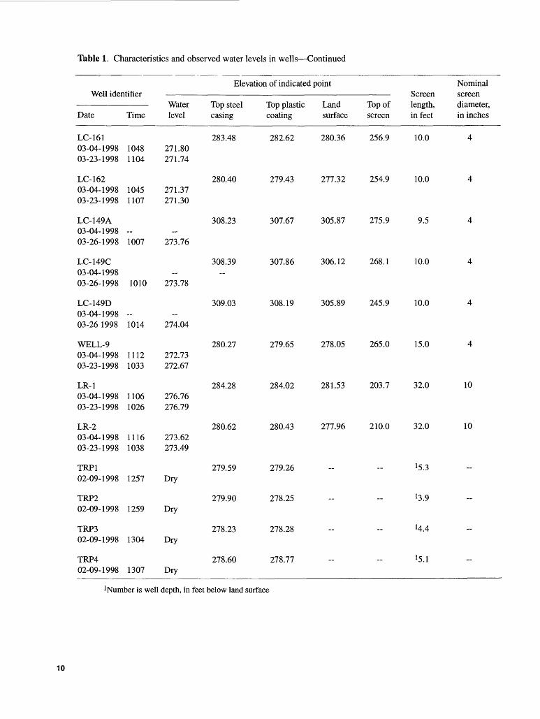
Table 1. Characteristics and observed water levels in wells Continued
Well identifier
Date
LC-16103-04-199803-23-1998
LC-16203-04-199803-23-1998
LC-149A03-04-199803-26-1998
LC-149C03-04-199803-26-1998
LC-149D03-04-199803-26 1998
WELL-903-04-199803-23-1998
LR-103-04-199803-23-1998
LR-203-04-199803-23-1998
TRP102-09-1998
TRP202-09-1998
TRP302-09-1998
TRP402-09-1998
Time
10481104
10451107
-1007
1010
1014
11121033
11061026
11161038
1257
1259
1304
1307
Elevation of indicated point NominalQ(->f£Wat1 C(->«V»0«
Water Top steel level casing
283.48271.80271.74
280.40271.37271.30
308.23~
273.76
308.39._
273.78
309.03
274.04
280.27272.73272.67
284.28276.76276.79
280.62273.62273.49
279.59Dry
279.90Dry
278.23Dry
278.60Dry
Top plastic Land Top of length, diameter, coating surface screen in feet in inches
282.62 280.36 256.9 10.0 4
279.43 277.32 254.9 10.0 4
307.67 305.87 275.9 9.5 4
307.86 306.12 268.1 10.0 4
308.19 305.89 245.9 10.0 4
279.65 278.05 265.0 15.0 4
284.02 281.53 203.7 32.0 10
280.43 277.96 210.0 32.0 10
279.26 -- - 1 5.3
278.25 - -- !3.9
278.28 - - 14A
278.77 -- -- I 5.l
1 Number is well depth, in feet below land surface
10

On the February dates, conductance profiles were measured, and water samples were collected from most of the 16 observation wells in the test area and three other wells (LC-149A, C, and D, fig. 2) located upgradient from the test area. On March 3, a few hours before the start of the test, conductance profiles were measured in the 16 observation wells.
A vertical profile of specific conductance in a well was obtained by lowering a probe into the well and manually recording the data at 1- to 3-foot intervals within the screened interval of the well. A water sample was obtained by lowering a submersible electric pump to the center of the screened interval of the well, purging the well by pumping a volume of water equal to about three times the volume in the screened interval of the well, and then collecting the sample. An exception to this procedure was for well LR-2, the inactive recharge well. Because this well has a 10-inch- diameter screen that is 30 ft long, it was impractical to pump, store, transport, and dispose of three screen volumes (about 350 gallons) from this well. Only about 20 gallons of water was pumped from this well before taking a sample on each of 3 days. The specific conductance of a sample was measured within a few minutes of the time it was collected.
About one month after the end of the test the samples were filtered through a 0.45-micron filter and sent to the U.S. Geological Survey Field Support Unit in Ocala, Florida, for bromide and chloride analyses. Aliquots of selected samples were sent to the U.S. Geological Survey National Water Quality Laboratory in Arvada, Colorado, for quality assurance. Concentrations determined by the two laboratories agreed well (table 2), as did specific conductances determined in the field and in the laboratories (not shown).
The passive method of obtaining vertical profiles of specific conductance is only appropriate if the ambient flow of water through the well screen is sufficient to purge the screened interval in a much shorter time than is needed for changes in conductance or concentrations in the ground water. Given the relatively high permeability of most of the sediments in the study area, this requirement is probably met.
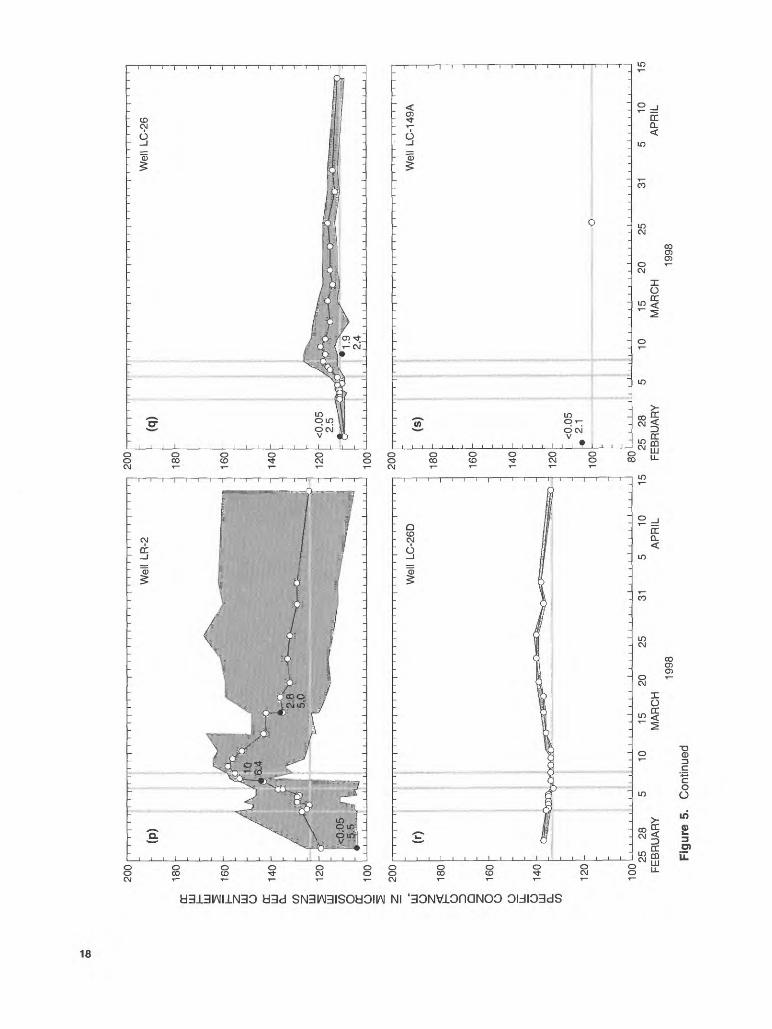
Analyses of Specific Electrical Conductance Data
To put the specific conductance data into a form useful for estimating hydraulic conductivities and dispersivities, each observed vertical profile was vertically averaged, and the average, maximum, and minimum values (table Al, in Appendix) were plotted as functions of time (fig. 5). The centroid (average time of arrival) and variance (a measure of longitudinal spreading) of the temporal distributions of excess vertically averaged conductance (conductance above the ambient level) were calculated (table 3) for use in computations of ground-water flow velocities, hydraulic conductivities, and dispersivities as described in the following subsections. The vertical conductance profiles themselves were not used because a vertical profile in a well could differ from the vertical profile in the ground water because of vertical flow in the well caused by differences in ground-water head over the screened interval (see, for example, Church and Granato, 1996). (If there are differences in ground- water head within the screened interval of a well, then ground water from zones with the greatest head would flow into the well, flow vertically within the well to zones where ground-water head is smallest, and flow back into the ground-water system there. Therefore, the conductance of water in a well probably is more representative of the ground water in the zones with the largest heads rather than an average over the entire screened interval. On the other hand, when water is pumped from a well for a length of time at a rate large enough to lower the water level in the well sufficiently below the minimum ground-water head within the screened interval, then more of the pumped water would come from zones with the larger hydraulic conductivity than from zones with the smaller hydraulic conductivity.) Because water samples for determinations of bromide and chloride concentrations were collected only a few times during the test, these data were insufficient for defining the temporal distribution of tracer at each well (fig. 5). However, the bromide and chloride data were used to assist in interpreting and verifying the conductance data.
11

Table 2. Concentrations of bromide and chloride, and specific electrical conductances of water samples
[Unless otherwise indicated, sample analyzed by laboratory at U.S. Geological Water Quality Services Unit (WQSU), Ocalla, Florida; *, Replicate of proceeding sample in table analyzed at WQSU laboratory; **, Replicate of preceeding sample in table analyzed by U.S. Geological Survey National Water Quality Laboratory, Arvada, Calif.; ***, outflow from treatment tower of East Gate pump-and-treat plant without dosing with potassium bromide; <, less than]
Site identifier
A15
A30
A45
B15
C25
C40
Well-9
LC-145
LC-146
LC-147
Date
02-26-199803-04-199803-05-199803-07-199803-11-1998
02-26-199803-04-1998
02-26-1998
02-26-1998*
03-04-199803-05-199803-07-1998
02-26-199803-08-199803-16-1998
02-26-199803-10-1998
02-26-199803-04-1998
02-26-199803-08-199803-18-1998
02-26-199803-04-1998
**
03-04-1998
02-26-199803-18-1998
Time
09070925143609230940
09250937
0944
1015
173614490908
114511151023
11400908
16291000
140310570952
14251013
1710
14401156
Specific electrical conductance, in microsiemens per centimeter
133174186156140
117121
117
128
145161164
150167143
143150
122178
112112121
122167
168
106110
Concentration of indicated constituent, in milligrams per liter
Bromide
<.051435240.4
<.050.9
<.05
<.05.03
132528
<.05124.5
<.056.2
<.0535
<.051.05.5
<.052727.530
<.051.8
Chloride
2.62.72.72.72.8
2.52.5
2.4
2.52.32.42.42.4
2.82.92.7
2.82.7
2.92.4
2.42.52.4
2.42.42.32.4
2.52.6
12

Table 2. Concentrations of bromide and chloride, and specific electrical conductances of water
samples Continued
Site identifier
LC-148
LC-149ALC-149CLC-149D
LC-161
LC-162
LC-26
LR-1 1
LR-2
LR-2
EGAT***
Date
02-26-199803-04-199803-05-199803-06-1998
***
02-25-199802-25-199802-25-1998
02-27-199803-10-1998
02-27-1998
02-26-199803-09-1998
03-05-199803-06-1998
02-26-1998*
****
03-07-1998
***
03-16-1998
04-14-1998
Time
1456171514230920
162516591640
15520848
1625
14370923
06350730
1657
1000
0939
0758
Specific electrical conductance, in microsiemens per centimeter
117132134140
105116112
128132
239
111110
1922200
104
144
136
119
Concentration of indicated constituent, in milligrams per liter
Bromide
<.057.8
12151516.3
<.05<.05<.05
<.05<.05
<.05
<.051.9
3840
<.05<.05
.04
.0410
1010.72.8
0.1
Chloride
2.42.42.42.42.42.4
2.12.42.3
2.32.4
2.9
2.52.4
6.32.8
5.55.55.55.66.4
6.36.25.0
2.5
1. Sample from well LR-1 without dosing with sodium chloride (NaCl).
2. Specific conductance of sample taken at 0655.
13

£U
U
180
DC LU t p
160
LU O £
140
CL C/D Z LU ^
12
0LU C/D O DC
, ,
, i
, ,
, ,
,.,
, ,
, i
, ,
, ,
i ,
, ,
, i
, ,
, ,
i ,
, ,
, ,
i ,
, ,
, i
, ,
, ,
i ,
, ,
,
- (a
) T
reat
men
t P
lant
-
outfl
ow- -
-
-
- ,- 0 0
- - _
i ,
, i
i
- -*
i
1 _
_^\
.»
.-
.
» *
1j
,,
I ',,',,
I ,,,,,,,,,
1 ,,,,
1 ,,,,,
I ,,,,
1 ,,,,,,,,,"
iLiL
\J
200
180
160
140
H O
A
, ,
, i
, ,-,
,
,.,
, ,
, i
, ,
, ,
i ,
, ,
, i
, ,
, ,
, ,
, ,
, ,
i ,
, ,
, ,
, ,
, ,
i ,
, ,
,
- (b
) j
Gal
lery
5 a
nd L
R-1
-
99 '
(with
out
NaC
I)*
'
- _ - - _
-
« __
S
. ., i .
"i i , i
, i i.r
.t 0i
, i* 1
1 , i ,
,"",",'"7
,,,,,,
, rrr*
'< < >
< < < -
> < < <
<~O
10
0
i^u
^
25
28
5 10
15
20
25
31
5 10
15
Z
200
^ LU
0 Z <
180
0 =)
O z O
160
0 0 LL O.
. _
140
LU
HU
0_
C/D
12
0
100
i *
* i
i i
i i
i i
i - 1
i i
i i
i i
i i
i i
i i
i i
i i
i i
i i
i i
i j
i i
i j
i i
i i
i i
i i
i~
, 1
24/
\ 3
-5
A
~ (C
) 2
.7;$
» * i y:
2.^* - - - <
005 ^
\
l
2-7
well
A15
- - -
.0.4
\ V 9
fli
s
14
'A
i
a ^
^M.^
~2
.'.6
.Jr?
> ~
IkJ
1 '^
Q'W
a^""
"*
&
V"\X
^ 7*
^-^
fiE
&&
S&
^tt
%\
~
-i*r
. - - -
_ -i
1 ,
, 1
1 ,
1 1
1 1
! 1
1 I
1 1
, 1
1 1
1 ,
1 1
1 1
1 1
1 1
1 1
1 1
1 1
1 1
1 1
1 1
1 1
1 1
1 1
FE
BR
UA
RY
M
AR
CH
A
PR
IL19
98
EX
PLA
NA
TIO
N
Spe
cific
con
duct
ance
in
vert
ical
pro
file
Min
imum
to
Max
imum
-o
"
Mea
n
Spe
cific
con
duct
ance
of
sam
ple
with
bro
mid
e (u
pper
num
ber)
and
chlo
ride
(low
er n
umbe
r)co
ncen
trat
ions
, in
mill
igra
ms
per
liter
5.6
2.4
j f A
mbi
ent
spec
ific
cond
ucta
nce
i i
25
28
5 10
15
20
25
31
5
10
15
!F
EB
RU
AR
Y
MA
RC
H
AP
RIL
S
tart
and
end
E
nd o
f N
aCI
1998
of
KB
r do
sing
do
sing
Figu
re 5
. S
peci
fic e
lect
rical
con
duct
ance
s, a
nd b
rom
ide
and
chlo
ride
conc
entra
tions
in
wel
ls a
s fu
nctio
ns o
f tim
e.

SPECIFIC CONDUCTANCE, IN MICROSIEMENS PER CENTIMETER

SPECIFIC CONDUCTANCE, IN MICROSIEMENS PER CENTIMETER

DC
LLJ
200
180
j=
160
Z HI O E
14
0
Q_
CO Z 5
120
UJ CO S O
100
200|-
rr-r
HI
O I Q O
O g LL
O 0_
CO
180
160
140
12
0
100
(n)
25
28
FE
BR
UA
RY
1015
20
M
AR
CH
1998
25
31
Wel
l LC
-146
Wel
l LC
-147
200
180
160
140
120
100
200
180
160
140
120
100
<0.
05
2.9
5 10
15
25
28
5
AP
RIL
F
EB
RU
AR
Y10
15
20
25
M
AR
CH
1998
Wel
l LC
-148
-
31
5 10
15
A
PR
IL
Figu
re 5
. C
ontin
ued
Ql
SPECIFIC CONDUCTANCE, IN MICROSIEMENS PER CENTIMETER
<nc
Ol
O o
cCD QL
oIT
TJ 3J
-i i i | i i i | i i i | i i i I i i r
11o : ro - en . O
-n co o i\3 [* en oo m , ° ° ° ° ° ° -i i i ^ i
Aroo ^b
i i i i i i i i i
O
i i i i i i i u

*;u
u
CC HI
1-
Hl
.^
180
HI ^
o t
;
& 0
16
0
o£
QC
/D
140
°S
o ^
U_
HI
12
0O
CO
H
I O
Q_
CC y
100
z ~o
n
_'
' '
' '
'
: (t)
- _ - - - - ; <o.o
5-
2.4
*
- - _
l l
l I
l l
oU
25
28
FE
BR
UA
RY
1
i i
i5
' '
' '
' '
' '
' '
' '
' '
' '
' '
' '
' '
' '
' '
' '
' '
' '
' '
' '
' '
Wel
l LC
-149
C~ - - - _ - ~
o
,
, ,
- - ~i
i i
i i
i i
i i
i i
i i
i i
i i
i i
i i
i i
i i
i i
i i
i i
i i
i i
i i
i
£.\j\
j
180
160
140
120
100
on
(m
i- - - ~ - -
|-
<0.0
5-
2.3
- -
i i
l I
l l
l I
I
10
15
20
25
31
5 10
15
25
28
5
MA
RC
H
AP
RIL
F
EB
RU
AR
Y19
98
, 1
1,1
11
,
i ,
, , ,,,
i ,,,,,,,,,,,,,,,,,,,,,,,
Wel
l LC
-149
D" - - - . - " ~ "
; -
"
i i
i i
i i
i i
i i
i i
i i
i i
i i
i i
i i
i i
i i
i i
i i
i i
i i
i i
i i
i i
10
15
20
25
31
5 10
15
MA
RC
H
AP
RIL
1998
Figu
re 5
. C
ontin
ued

Table 3. Computed centroids and standard deviations of temporal distributions of observed vertically averaged values of specific electrical conductance in excess of ambient values
[--, value not determined]
Siteidentifier
Gallery 5and 6
A15A30A45
B15
C25C40
WELL-9LC-145LC-146LC-147LC-148
LC-149ALC-149CLC-149D
LC-161LC-162
LC-26LC-26D
LR-1
LR-2LR-2
Ambient specificplpptripj}!V'll/^l.l It^dl
conductancein microsiemensper centimeter
125140116117
124
_134
123112123106119
100116114
132224
111134
-
124124
Estimate when specific electrical conductance returns to ambient value
Month-dayin 1998
03-0603-0804-1404-14
03-15
_04-10
03-1004-1403-1004-0903-13
_ -
_-
04-1404-14
03-08
04-1403-25
Time
1020023008480851
0000
_0000
07320818072808001332
_ -
_-
08360840
1030
08270827
Centroid
Month-dayin 1998
03-0403-0503-2603-27
03-07
_03-21
03-0503-2203-0503-2203-07
_~
_~
03-2103-26
03-05
03-1603-12
Time
2250191305372219
1714
_0050
07102159200522410137
_
_-
20051652
1200
22121231
Hours since03-01-1998,0000
94.8115.2605.6646.3
161.2
_480.3
103.2527.8116.1526.7145.6
_
_-
500.1616.9
!108
382.2276.5
Standard deviation(square rootof variance),in hours
20.822.7
189.9191.6
46.9
_199.7
23.0143.226.1
172.140.7
_~
__
247.2177.7
-
216.0106.3
Assumed value.
20

Hydraulic Conductivity
Hydraulic conductivity is a measure of the capability of a porous medium to transmit water. The conductivity is a function of the viscosity and specific weight of the water and of the size, shape, and connectivity of the pores in the media through which the water flows. In sedimentary geologic formations, the geometry of the pores is a function of the size, shape, and packing of the sediment particles. In formations with horizontal bedding, the effective gross hyditaulic conductivity of a geologic unit usually is larger in the horizontal than in the vertical direction because of layers with different particle sizes within the unit and the orientations of individual particles.
Hydraulic conductivity, K , can be computed by applying variations of Darcy's law between pairs of observation wells (see, for example, Freeze and Cherry, 1979). Two expressions are derived here, one for steady uniform rectilinear flow and another for steady axially symmetric radial flow away from a recharge well. For uniform rectilinear flow with uniform K ,
In areas of primarily horizontal flow, equation 3 can be used to estimate the horizontal hydraulic conductivity Kh of the material between the wells. For this case the observation wells must be screened at about the same depth in the same geohydrologic unit, and L is the horizontal distance between the wells. In areas of primarily vertical flow, equation 3 can be used to estimate vertical hydraulic conductivity, Kv In this case the horizontal distance between the observation wells must be small, and L is the vertical distance between the midpoints of the screened intervals of the wells. If two wells are separated both horizontally and vertically, or if flow is not primarily vertical or horizontal and the hydraulic conductivity is not isotropic, equation 3 is not suitable for estimating hydraulic conductivity.
An expression similar to equation (3) for horizontal radial flow away from a recharge well is also needed. The discharge per unit thickness, q, away from a well in a radial direction, r, is given by the differential equation:
V = (1)
where v is the so-called average linear velocity (Freeze and Cherry, 1979, p. 71); n is the effective porosity; Ah is the difference between water levels (hydraulic heads) at two locations separated by a distance L parallel to the flow direction. The velocity, v, can be approximated by
LAt
(2)
where At is the average travel time between the two locations. The At can be estimated as the difference between the computed centroids of the temporal distributions tracer concentration or excess specific conductance. Substituting equation 2 into equation 1 and solving for K yields
K =-nVAtAh
(3)
q = -Kh2nr ,dh dr
which, when integrated, gives
q = -2nKf Ah (4)
where Ah is the difference between heads at radii r2 and r t . The equation for travel time is
, dr dt = =v
dr
L(2nrn)_
(5)
Substituting equation 4 into this equation, integrating, and solving for Kh yields
Kh = -n(2AtAh)
21

Longitudinal Dispersivity
Longitudinal dispersion is the mixing of dissolved material in the direction of flow by the combined effects of differences in flow velocity along different flow paths and cross-wise mixing between the flow paths (see, for example, Fetter, 1993). A mathematical analysis of this process reveals that transport per unit area by longitudinal dispersion can be computed as the product of a longitudinal hydrodynamic dispersion coefficient and the longitudinal gradient of the concentration averaged over an area perpendicular to the flow velocity. The value of this dispersion coefficient increases with the variation in velocity within the area and the dimensions of the area, and it decreases with the intensity of crosswise mixing within the area. Consequently, the value of the dispersion coefficient is dependent on the area over which it is defined. For example, the longitudinal dispersion coefficient in the horizontal direction for a combined sequence of coarse- and fine grained geologic units with horizontal bedding would be much larger than the dispersion coefficient for any of the individual units because the variation in flow velocity within the sequence would be larger than the variation within any of the individual units, and the thickness of the sequence would be larger than the thickness of an individual unit. Dispersion coefficients for directions perpendicular to the flow velocity, often referred to as transverse dispersion coefficients, are the result of different processes and normally are smaller than the longitudinal dispersion coefficient.
In order for the concept of a longitudinal dispersion coefficient to be valid (flux by longitudinal dispersion equals the product of a dispersion coefficient and longitudinal concentration gradient), sufficient time must elapse after the introduction of a material into the flow system for each parcel of material to migrate across the entire area for which the dispersion coefficient is defined. For times shorter than this, the apparent dispersion coefficient will be less than the ultimate value.
Dispersivity is a coefficient with units of length that relates a hydrodynamic dispersion coefficient to ground-water velocity (Freeze and Cherry, 1979, p. 389-399). For the longitudinal dispersion coefficient, one can write
where DL is the longitudinal hydrodynamic dispersion coefficient, and aL is the longitudinal dispersivity. Often, to obtain the total longitudinal dispersion coefficient, a term to account for molecular diffusion is added to DL ; however, in most cases, including the present investigation, this term is many factors of 10 less than DL and is neglected.
The longitudinal dispersion coefficient and the dispersivity can be calculated from the rate of longitudinal spreading of a tracer. If a tracer is being transported in a uniform steady rectilinear velocity field, the dispersion coefficient may be computed as
(7)
d<3,Lwhere is the time rate of change in the variance
of the longitudinal (spatial, in the direction of flow) distribution of concentration of the tracer (see, for example, Fischer and others, 1979, p.41). (Here, DL is defined such that the dispersive flux per unit gross area is equal to the product nDL times the concentration gradient, while some investigators define DL such that the flux is equal to DL times the concentration gradient. In the latter case, the values of the dispersion coefficient and dispersivity would be n times the values obtained in the present study.)
In this as in most investigations, the available data consist of temporal rather than the needed spatial distributions of tracer. To obtain <5L for use in equation 7, the variance of the temporal distribution, Gt , is multiplied by the square of the velocity, v . When the time derivative in equation 7 is replaced by the difference between values at two observation locations divided by the travel time between the locations and equation 2 is used for the velocity, equation 7 becomes
9 7L AG,
2(A03(8)
DL = aLv (6)
22

Substituting equations 8 and 2 into equation 6 and solving for the dispersivity yields
LAaa, = (9)
GROUND-WATER FLOW DIRECTIONS
In this section observed ground-water levels are presented and used to infer directions of ground-water flow in the test area. This section also presents and describes observed temporal and spatial distributions of specific conductance, and bromide and chloride concentrations and relates them to the flow directions inferred from water levels.
Ground-Water Levels and Flow Directions
Water levels in wells within the test area were measured twice during the tests, once near the beginning of the test on March 4, 1998, and again on March 23, 1998. All measured water levels, except in upgradient wells LC-149A, C, and D, were less than 10 ft below land surface. Water levels declined slightly in the period between the two measurements and on March 23 were 0.01 to 0.10 ft lower than on March 4 in all wells except the recharge well (LR-1), where the water level was 0.03 ft higher (table 1). Although there are two shallow wells (4 to 5 ft deep) in each of the galleries (wells TRP1 through TRP4 on figure 4), water levels were below the bottoms of these wells. Consequently, water levels directly beneath the galleries are unknown. The water levels that form the basis for the discussions in the following paragraphs and those that appear on the accompanying figures are averages of the March 4 and 23 measurements. However, the interpretations of the data would not have changed if one or the other of these data sets were used instead of the average.
Directions of ground-water flow can be inferred from water levels because flow is in the general direction of decreasing water level, and average linear velocities can be estimated using equation 2 (figs. 4, 6, and 7, and table 4). The available data indicate that the flow field is complex, probably partly because of the heterogeneity of the sediment deposits and partly because of the withdrawal and recharge from the pump-and-treat system. Estimated velocities in the
horizontal direction ranged from 0.18 to 3.4 feet per hour and decreased along section AA' with distance from recharge gallery 5 (figs. 4 and 6). Most of the velocities in the vertical direction, which ranged from 0.083 to 2.0 feet per hour, were of the same order of magnitude as in the horizontal direction, probably because all of the former were beneath the recharge gallery. Although the data are not sufficient to completely define the flow field in the test area, some generalizations can be made. The data are sufficient to allow one to infer that near the water table there was a horizontal component of flow in the northwesterly direction along section AA' (figs. 4 and 6). This is consistent with previously inferred flow directions in the upper aquifer beneath the East Gate Disposal Yard and most of the Logistics Center (U.S. Army Corps of Engineers, 1998, fig. 5) and with the concept that ground water flows from the recharge to the extraction area of the pump-and-treat system. At a depth of about 80 ft below land surface, which is still within the upper aquifer, there was a horizontal component of flow from the active to the inactive recharge well (LR-1 to LR-2, fig. 7), as would be expected. However, at a depth of about 40 ft below land surface, at the elevation of the midpoints of the screened intervals in wells LC-145, LC-146, LC-147, and LC-148, the apparent horizontal component of flow was in the opposite direction (fig. 7). One possible reason for the different flow direction at 40-ft depth could be the slightly larger flow into gallery no. 6 (330 gpm) than into gallery no. 5 (270 gpm); other reasons include a spatial pattern or an anisotropy in the hydraulic conductivity.
One would expect that the vertical component of ground-water flow near the recharge galleries would be downwards near the water table, and near the recharge well would be upwards at depths slightly less than the center of the screened interval of this well. Flow directions near the water table, as inferred from water levels, are indeed down between WELL-9 and well LC-146, between A15 and A30, and between C25 and C40 (figs. 6 and 7). Because water levels in wells LR-1 and LR-2 are higher than in wells LC-145, LC-146, LC-147, and LC-148, the direction of the vertical component of flow between about 40 ft and 80 ft below land surface is most likely upward. The vertical component of flow between wells A30 and A45 is upward also.
23

300
28
0
260
LU LU uj
240
220
200
1 1
I
LO
CVJ o
A
At
=
271.
73 ItI '
I '
I
O
LO^^
r
1 1
' 1
' 1
LO
OL
O^J
* CO
"*""
O
< «
271.
66
_
i I
=
=
0.18
-*
I .
I i
I
t -
-Z_
1.5
271.
76
^ ___
I
.Z_1 ._
I i
I i
I i
i |
i |
i |
i
LO ^Q
.=
QC
,<S H
A
'CD
"*
i _
__
rT_
* -«-^""
w
^ 3.
4 ^
272.
01 i 1
271.
73
271.
> I
< I
i I
t 82
EX
PLA
NA
TIO
NLO ^
Wel
l id
entif
ier
-
^-J-
VT-^
La
nd s
urfa
ce
272.
01
"H=
Wat
er le
vel
Wat
er-
fle
vel
Ijn
fee
t S
cree
ned
inte
rval
abov
e I
sea
leve
l _
I
15
Flow
dire
ctio
n, a
nd-*
velo
city
in f
eet
per
hour
whe
re e
stim
ated
I i
I i
I i
i I
i I
i I
.20
010
0H
OR
IZO
NT
AL
DIS
TA
NC
E,
IN F
EE
T
-100
Figu
re 6
. S
ectio
n al
ong
a lin
e th
roug
h w
ells
C25
and
TR
P-2
sho
win
g el
evat
ions
of w
ell s
cree
ns,
obse
rved
wat
er le
vels
, an
d in
ferr
ed g
roun
d-w
ater
flow
di
rect
ions
and
est
imat
ed v
eloc
ities
, Fo
rt Le
wis
, Was
hing
ton.
Wat
er le
vels
are
ave
rage
s of
obs
erva
tions
on
Mar
ch 4
and
23,
199
8.

LLJ u
300
280
260
240
5
220
_i LU
200
180
160
1
T D
B\\
- - ~ -
i
i
: j
77-
_2.
t
1
LO 6 _l
sv
U
«-
' 1 t_
_z.
1
I i
I i
i |
i |
i |
6
- »
...
Gal
lery
5
, *'«
..'
0.79
27
1.6
9
276.
78
i1
I1
i
1 "-
272.
32
EX
PLA
NA
TIO
NC
D jj
Wel
l ide
ntifi
er
-*-»
-Kr-
»-
Land
sur
face
272.
70 ft
Wat
er le
vel
Wat
er-
? le
vel
1 in
fee
t S
cree
ned
inte
rval
ab
ove
1 se
a le
vel
|
P n
1 Fl
ow d
irect
ion,
and
1
velo
city
in fe
et p
er
T ho
ur w
here
est
imat
ed
1 i
i 1
> 1
i
_z. 2.
0
1.6
1 1
c L *
U'
I '
I '
I '
I '
|> J J LJ >
>
".'
- \
».- '*
'
Gal
lery
6
'. »-
'.
27
2.7
0
L 0.
083
)
I '
r-.
Q"t
CD
C
D
T-
CM
CM
66
6
^~r
272
272.
44
>-
I i
I i
I i
I i
,32 j.
t
270.
22 149
-1
139
-
I i
i
C\J
DC
B1
z__z
.
- ~
273.
56
-
i
030
010
0 20
0H
OR
IZO
NT
AL
DIS
TA
NC
E,
IN F
EE
T
Figu
re 7
. S
ectio
n al
ong
a lin
e th
roug
h w
ells
LR
-1 a
nd L
R-2
sho
win
g el
evat
ions
of w
ell s
cree
ns,
obse
rved
wat
er le
vels
, an
d in
ferr
ed g
roun
d-w
ater
flow
di
rect
ions
and
est
imat
ed v
eloc
ities
, Fo
rt Le
wis
, Was
hing
ton.
Wat
er le
vels
are
ave
rage
s of
obs
erva
tions
on
Mar
ch 4
and
23,
1998
.

Tab
le 4
. Est
imat
ed v
alue
s of
hyd
raul
ic c
ondu
ctiv
ities
and
lon
gitu
dina
l di
sper
sivi
ties,
and
dat
a us
ed to
com
pute
the
m
[1 an
d 2,
up-
grad
ient
and
dow
n-gr
adie
nt s
ites,
resp
ectiv
ely;
h a
nd v
, hor
izon
tal a
nd v
ertic
al d
irect
ions
, res
pect
ivel
y; h
oriz
onta
l coo
rdin
ates
, exc
ept f
or s
ites
LR-1
and
LR
-2, a
re
north
wes
t fro
m a
line
thro
ugh
wel
ls L
R-1
and
LR-2
and
par
alle
l to
line
thro
ugh
wel
ls A
15 a
nd C
25, f
or L
R-1
and
LR
-2 c
oord
inat
es a
re r
adia
l dis
tanc
e fr
om c
ente
r of w
ell L
R-1
; ve
rtica
l coo
rdin
ates
are
ele
vatio
ns a
bove
sea
leve
l; gr
ound
-wat
er h
ead
is av
erag
e of
obs
erva
tions
on
Mar
ch 4
and
Apr
il 23
,199
8; C
entro
id is
mea
sure
d fr
om 0
000
hour
s on
M
arch
1,1
998;
<, l
ess
than
; >, g
reat
er th
an;
--, v
alue
not
det
erm
ined
]
Iden
tifie
r of
indi
cate
d si
te
1
Gal
lery
5G
alle
ry 5
A15
B15
B15
Gal
lery
6G
alle
ry 6
Gal
lery
6G
alle
ry 6
LR-1
LR-1
Gal
lery
5G
alle
ry 5
Gal
lery
6
WE
LL
-9
Gal
lery
6G
alle
ry 6
2
A15
A15
B15
C25
C40
LC
-148
LC
-148
LC
-26
LC
-26
LR
-2LR
-2
LC
-145
LC
-145
WE
LL
-9
LC
-146
LC
-147
LC-1
47
Dir
ectio
n
h h h h h h h h h h h V V V V V V
Hyd
raul
ic
cond
uctiv
ity,
in f
eet p
er d
ay
>840
<2,4
00
3,10
0
2,30
054
0
>260
<3,1
00 >69
<490
3,80
02,
300 >8 <19
>110 59
0 >8 <80
Lon
gitu
dina
di
sper
sivi
ty
in f
eet
6.9
- 28 __ 9.1
16 - 19 - __ - 1.8
- 12 9.1
2.8
-
Coo
rdin
ate
of in
dica
ted
il si
te, i
n fe
et
1
-24
-24 45 115
115 8 8 8 8 0.
50.
5
274
274
275
258
275
275
2 45 45 115
170
164 76 76 -94
-94
300
300
240
240
258
238
239
239
Gro
und-
wat
er
head
at i
ndic
ated
si
te, i
n fe
et
1
!<27
42>
272.
70
272.
01
271.
7627
1.76
!<27
52>
272.
70
!<27
52>
272.
70
276.
7827
6.78
1<27
42>
272.
70
1<27
5
2272
.70
!<27
52>
272.
70
2
272.
0127
2.01
271.
76
271.
7327
1.66
272.
4927
2.49
272.
3227
2.32
273.
5627
3.56
271.
6927
1.69
272.
70
272.
32
272.
4427
2.44
Cen
troi
d at
in
dica
ted
site
, in
hour
s
1
94.8
94.8
115.
2
161.
216
1.2
94.8
94.8
94.8
94.8
4108
4108 94
.894
.8
94.8
103.
2
94.8
94.8
2
115.
211
5.2
161.
2
3480
.348
0.3
145.
614
5.6
500.
150
0.1
276.
638
2.2
527.
852
7.8
103.
2
116,
1
526.
752
6.7
Gro
und-
w
ater
ve
loci
ty,
in f
eet
per
hour
3.4
3.4
1.5
0.18
0.18
1.4
1.4
0.25
0.25
__ - 0.79
0.79
2.0
1.6
0.08
30.
083
Stan
dard
dev
iatio
n at
indi
cate
d si
te,
in h
ours
1 20.8
- 22.7
46.9
46.9
20.8
- 20.8
-- _ - 20.8
- 20.8
23.0
20.8
-
2 22.7
- 46.9
..19
9.7
40.7
-
247.
2-
106.
321
6.0
143.
2~ 23
.0
26.1
172.
1-
App
roxi
mat
e el
evat
ion
at b
otto
m o
f gal
lery
. 2W
ater
leve
l in
WEL
L-9.
3C
entro
id is
from
dat
a at
wel
l C40
. 4E
stim
ated
.

The complexity of the inferred flow patterns in the test area would make the design and evaluation of most remediation methods and the interpretations of observed contaminant distributions difficult. Those doing these tasks should be cautious and aware of the complex patterns of ground-water movement that are possible in this environment.
Bromide and Chloride Concentrations
Bromide, but not chloride, concentrations in samples collected from most wells during the test were higher than ambient concentrations in samples collected about one week before the test, indicating that most of the observed increases in electrical conductance in water in wells during the test (see the subsection "Specific Electrical Conductance") were the result of the KBr tracer in the water from the recharge galleries. (See also the plot of specific conductance as a function of bromide concentration on fig. Al of the Appendix.) The ambient concentrations of bromide in samples from all 15 sampled observation wells in the test area and the three upgradient wells were less than 0.05 mg/L (table 2 and fig. 5, samples collected on February 25, 26, or 27). The bromide concentration was 0.9 mg/L or more in at least one sample from all but one of the 13 observation wells that were sampled during the test (table 2 and fig. 5, samples collected on or after March 4). The largest concentration (35 mg/L) was in a sample from well A15, which is nearly equal to the observed concentration in recharge water, as represented by the samples from well LR-1 (38 and 40 mg/L, table 2). No samples were taken during the test from wells A45 or LC-162, and the one sample taken from well LC-161 during the test may have been taken before the tracer reached this well.
Ambient chloride concentrations in samples from all wells (with the exception of LR-2) ranged from 2.1 to 2.9 mg/L. Concentrations in the samples collected during the test from all wells but LR-2 were no more than 0.2 mg/L greater than the ambient concentrations, and concentrations in samples from seven of the wells were the same or lower than ambient levels (table 2 and fig. 5).
Chloride concentrations in samples from well LR-2 suggest that some of the water in this well was injected at well LR-1 as would be expected because both wells are screened at nearly the same elevations (fig. 7). However, anomalies in the chloride
concentrations in samples from this well preclude drawing definite conclusions. Although the bromide concentration in the sample collected from well LR-2 one week before the test was about the same as the concentrations in samples from the other observation wells (<0.05 mg/L), the chloride concentration was 5.5 mg/L, which is about twice that in samples from the other wells (table 2). On March 7, when the bromide concentration increased to 10 mg/L, the chloride concentration was 6.4 mg/L, about 1 mg/L larger than before the test (table 2 and fig. 5; note that the concentrations in the samples collected from well LR-2 on February 26 and March 7 were verified by analyses of replicate aliquots of the sample at two laboratories). On March 16, when the bromide concentration decreased to 2.8 mg/L, the chloride concentration decreased to 5.0 mg/L, which is 0.5 mg/L or 9 percent smaller than before the test. The reasons for the anomalies in the chloride concentrations in the samples from well LR-2 are unknown, but are suspected to be a result of inadequate purging of this well before sample collection (see the "Monitoring" subsection in the "Methods" section).
Specific Electrical Conductance
The effect of the KBr tracer on the specific conductance of the ground water and the usefulness of electrical conductance for monitoring the movement of the tracer are evident in the graphs of vertically averaged conductance as functions of time (fig. 5). In each sample collected the bromide but not the chloride concentration was elevated whenever the electrical conductance that was measured in situ was elevated (fig. 5). The specific electrical conductances of samples from most wells are about the same as the vertically averaged specific conductances measured in situ (see data for wells A15, LC-145, LC-146, LC-147 and WELL-9 on figs. 5c, k, 1, m and n, respectively). However, sample conductances differ from the vertically averaged in-situ values for some wells, and some even lie outside the range of values in the in-situ vertical profile (see data for wells B15, C25, C40 and LC-26 on figs. 5f, g, h, and r, respectively). As stated earlier, the average of a vertical profile of a characteristic of water in a well and the characteristic of a sample taken from the well can differ because of vertical flow within the well induced by differences in hydraulic heads within the well's screened interval and
27

differences in horizontal hydraulic conductivity within the screened interval.
The ambient values of specific conductance varied among the wells, with time, and with depth within the screened intervals of some wells. Although most ambient values were between about 105 and 125 |u,S/cm, the entire range was from about 100 |u.S/cm at well LC-149A to greater than 200 ^.S/crn at LC-162 and greater than 400 |u,S/cm at well C25. Some of the variation in ambient specific conductance among wells is probably natural, but the larger conductances probably are a result of local dissolution of materials buried in the disposal yard. For example, on March 26 the values of vertically averaged in-situ specific conductance at wells LC-149A, C, and D, which are within a circle of 20 ft radius and are screened at increasing depths between 30 and 80 ft below land surface, were 100, 119, and 114 uS/cm, respectively (figs. 5s, t and u, and Appendix A). (Values of specific conductance of samples collected from these wells on February 25 had a similar but slightly smaller variation, 105, 116, and 112 n,S/cm, table 2.) The differences between the vertically averaged value for well LC-149A and the other two wells are much greater than the observed variation with depth within any of these wells, even though these wells are upgradient of any suspected contamination. On the other hand, reported concentrations of TCE in samples from well LC-162 have been as large as 1,000 |U.g/L (Woodward- Clyde, 1998, table 2-3B), suggesting that the elevated ambient specific conductance of the water in this well may be the result of local contamination. Also, the large values of specific conductance observed at some levels in well C25 probably can be attributed to a local contaminant source because an oily substance was encountered when drilling the hole to install this well.
Differences between values of specific conductance measured in-situ 1 week before, a few hours before, and at the end of the test are an indication of the temporal variations in ambient electrical conductance. At most locations observed temporal changes in ambient specific conductance are of the order of the estimated accuracy of the measurements (a few microsiemens per centimeter) (wells A45, LC-145, LC-146, LC-147, and WELL 9 on figs. 5e, k, 1, n, and m). However, at a few locations the apparent variation was as large as 10 |u,S/cm (well A15, fig. 5c).
The movement of tracer from recharge gallery 5 to the northwest is evident from the observed electrical conductance at wells A15 and B15, which are screened
at the water table, and to a lesser extent at well C40, in which the top of the screen is about 18 ft below the water table. Presence of the tracer based on the specific conductance at well C25, which is screened at the water table and is adjacent to C40, is difficult to discern because of the large variation in the ambient conductance, as described previously. However, the bromide concentration in the sample collected from well C25 on March 16 (4.5 mg/L) indicates the presence of the tracer at that location. The conductance at wells LC-161 or LC-162 (figs. 5i and j), which are the farthest downgradient observation wells, hints at the presence of tracer; however, the changes in conductance are small and there are no bromide data for verification.
Even though wells LC-26 and LC-26D are upgradient (with respect to the regional flow system) of the recharge galleries and recharge well, the recharge of the water through the galleries and well apparently reverses the gradient locally, and some of the recharged water moved from the galleries to LC-26 and perhaps to the deeper well LC-26D. The presence of tracer at LC-26 is indicated by an increase in specific conductance of about 10 |u,S/cm, which is confirmed by a bromide concentration of 1.9 mg/L in a sample collected on March 9 (fig. 5q and table 2). No bromide data are available to verify that the increase in conductivity at LC-26D (fig. 5r) was caused by arrival of the tracer.
Data from wells with screens that are entirely below the water table suggest there is large spatial variability in the downward movement of the tracer. At wells A30 and A45, which are adjacent to A15 but screened 0 to 15 ft and 15 to 30 ft deeper than well A15, respectively (table 1), observed values of specific conductance increased no more than about 5 |u,S/cm above background (figs. 5d and e). The magnitudes of these increases are near the magnitudes of the variations in ambient conductance and the estimated magnitude of the error in the determinations of specific conductance. However, a bromide concentration of 0.9 mg/L in the sample from well A30 (fig. 5d and table 2) indicates that the tracer was present in this well. No sample was collected from well A45; however, the fact that the water level in well A45 is about 0.1 ft higher than in A30 indicates that tracer could not be moving downward from well A30 to A45 at this location. Wells LC-145, LC-146, and LC-147 are all located on a line near and approximately parallel to the two galleries, and all are screened at similar
28

depths from about 30 to 50 ft below land surface (figs. 4 and 7). Well LC-148 also is screened at about the same depth but is about 75 ft northwest of the line, and WELL-9 is on the line but is screened at a shallower depth (13 to 28 ft below land surface). Specific conductance in WELL-9, and in nearby well LC-146, increased by 50 |j.S/cm within two days after the start of the test and decreased to ambient levels by March 10, 5 days later (figs. 5m and 1). In well LC-148 conductivity also increased substantially, by about 35 |j.S/cm, and returned to near ambient levels by March 10. On the other hand, conductance in wells LC-145 and LC147 increased by only about 15 and 5 |j.S/cm, respectively, and did not appear to return to ambient levels until after April 2.
ESTIMATED HYDRAULIC CONDUCTIVITIES AND DISPERSIVITIES
Although the complexity of the ground-water- flow in the test area probably prohibits the application of equations 3, 5, and 9 at the scale of the test site, it will be assumed that the flow patterns at the scale of distances between observation locations are approximately rectilinear or radial and these equations will be used to estimate hydraulic conductivities and dispersivities from the observed specific conductances. The centroids and variances of the temporal distributions of excess specific conductance at selected locations were computed by numerical integration (table 3) and used with observed or estimated water levels in the equations to obtain the estimates (table 4). In some cases two values of hydraulic conductivity were estimated between a pair of locations because of an uncertainty in the water level or the centroid at one of the locations. A value of 0.3 was assumed for porosity. The estimated hydraulic conductivities are directly proportional to the assumed value of porosity (equations 3 and 5), but the estimated dispersivities are independent of porosity (equation 9).
Horizontal Hydraulic Conductivity
Estimated values of horizontal hydraulic conductivity of the sediments in the upper part of the upper aquifer, as computed with data from five pairs of locations, were between 69 and 3,100 ft/d (table 4). The lowest estimated horizontal hydraulic conductivities are between gallery 6 and well LC-26
(69 to 490 ft/d). The values for this pair of locations may be low because the top of the screen in LC-26 is below the water table and the time of arrival of the tracer at this well could have been delayed because ground water would have had to flow vertically as well as horizontally to reach this well. However, the top of the screen in well LC-148 also is below the water table but the hydraulic conductivies computed between gallery 6 and this well (260 to 3,100 ft/d) are more than three times those between gallery 6 and well LC-26.
The estimated horizontal hydraulic conductivity at a depth of about 80 ft below land surface, as obtained with data from the two recharge wells (LR-1 and LR-2), is 2,300 ft/day or 3,800 ft/day, depending on which value of the centroid at LR -2 is used (table 3). The uncertainty in the centroid is a result of the uncertainty in the time at which the specific conductance returned to the ambient value. These values of hydraulic conductivity are near or greater than the largest values estimated for shallower sediments near the water table.
Vertical Hydraulic Conductivity
Estimated values of vertical hydraulic conductivity, as computed with data from four pairs of locations, were between 8 and 590 ft/day (table 4), which, as would be expected, are considerably less than the estimated hydraulic conductivities in the horizontal direction. The ratio of estimated horizontal to vertical hydraulic conductivity appears to be of the order of 10 or 100. Although the ratio is difficult to quantify because of the large range in the estimates for each direction and because many of the values are only lower or upper limits, the magnitudes of the ratios appear to be similar to those found from aquifer tests (12 to 259). Values of vertical hydraulic conductivities were not obtained from model calibration because the upper aquifer was simulated as a single layer.
Horizontal and Vertical Longitudinal Dispersivities
Estimated values of longitudinal dispersivity in the horizontal direction range from 6.9 to 28 ft. In the vertical direction the values are smaller, 1.8 to 12 ft. The values in the horizontal direction are within the broad range of values found by others in field tests of similar scale in granular materials (Gelhar and others,
29

1985). Although Gelhar and others (1985) also summarize values of dispersivity in the vertical direction, those values are dispersivity in the vertical direction resulting from flow in the horizontal direction (transverse dispersivity). The vertical dispersivities estimated in the current study are for flow in the vertical direction (longitudinal dispersivity).
Estimated longitudinal dispersivity is larger in the horizontal direction than in the vertical direction probably because of the nearly horizontal layering of the sediments in the study area. As discussed earlier, longitudinal dispersion normally is the result of variations of flow velocity in directions perpendicular to the velocity. When the layering is nearly horizontal, horizontal velocities could vary appreciably within the vertical as a result of vertical variations in texture of the sediments, whereas vertical velocities would tend to be more uniform within horizontal planes because of the relative uniformity of texture within bedding planes.
Discussion and Applicability of Estimates
The largest values of horizontal hydraulic conductivity estimated from the tracer tests are larger than previous estimates for the East Gate area based on numerical model calibration (80 to 260 ft/day) or aquifer tests (16 to 330 ft/day), (see "Geohydrology" subsection of "Introduction"). The probable reason for the differences is that the values from the tracer test are biased toward highly conductive layers (probably less than about 10 ft in thickness) that occupy only part of the total aquifer thickness (about 100 ft), while the values from model calibration and aquifer tests are averages over the entire thickness, or a large fraction of the thickness, of the upper aquifer. The significance of these differences is that if a vertical sequence of geohydrologic layers of varying hydraulic conductivities in an aquifer is represented in a numerical model by a single layer with a vertically averaged hydraulic conductivity, the model would tend to underestimate the shortest travel times between locations if the locations are connected by lenses or layers of material with a high hydraulic conductivity (a preferred pathway), even though the simulated ground- water heads agree well with observations. However, the relatively high values of hydraulic conductivity obtained from the tracer test can only be incorporated into a model if individual layers within the aquifer are explicitly represented.
The values of horizontal longitudinal dispersivity obtained in this study probably are also representative mostly of flow through thin, highly permeable layers. Although the estimated values of dispersivity may have been increased a small amount by tracer migrating into and out of adjacent layers of less permeable material, the magnitude of this increase also is unknown. On the other hand, if the time scales of the test were too short for parcels of tracer to migrate across all zones within the layer with different flow velocities, the estimated dispersivity for the layer would be too small (see the discussion of longitudinal dispersion in the "Dispersivity" subsection of the "Methods" section). The values estimated from the tracer test probably are appropriate only for coarse grained units in numerical models in which these layers are represented individually and explicitly. If these units are grouped with other units of different hydraulic conductivity into one model layer, then the dispersivity of this larger model layer would need to be larger than that obtained from the current study because of the greater variation in flow velocity among the units within the layer and the greater thickness of the layer.
A number of factors affect the accuracies of the estimated hydraulic conductivities and dispersivities. These include (1) the assumption that the flow between observation locations was rectilinear or radial as was assumed in the derivation of equations 3, 5, and 9; (2) the assumption that the values of vertically averaged specific conductance measured over the screened interval inside the wells were equal to the vertically averaged values in the aquifer outside the well, and (3) the accuracy of the procedure used to obtain the centroids and variances of the distributions of specific conductance, which depends, among other things, on the accuracy of the estimated values of ambient conductance and the estimated tail of the distributions. This report makes no attempt to quantify the errors associated with the above assumptions and estimates.
Factors that can affect the applicability of the estimates are not knowing (1) the accuracy of the estimates, and (2) the thicknesses and lithologies of the layers for which the estimates were obtained. The latter factor is the result of a lack of detailed knowledge of the lithology of the screened intervals of the wells or the entire test area. However, as stated earlier, the estimated values probably are representative of layers of larger than average hydraulic conductivity less than about 10 ft thick.
30

SUMMARY AND CONCLUSIONS
From about 1946 to 1971 the U.S. Army disposed of trichloroethylene (TCE) and other wastes at its East Gate Disposal Yard near the Logistics Center of Fort Lewis in western Washington. As a result, a plume of TCE dissolved in ground water now extends downgradient (northwest) from the disposal yard. Two pump-and-treat systems, one close to the disposal yard and another near the fort boundary, were put in operation in 1995 to prevent migration of TCE from the disposal yard and from the fort to neighboring areas; however, additional remediation may be necessary. The upper aquifer in the area consists of about 100 ft of a complex distribution of layers and lenses of mostly glacial outwash gravels, outwash sands, and glacial till. The water table at the disposal yard is about 10 ft below land surface. Knowledge of the hydraulic characteristics of these sediments is necessary for use in numerical ground-water flow and transport models that are being used to design and evaluate alternatives for remediation of subsurface contamination at the site.
A tracer test that utilized the pump-and-treat system at the disposal yard was conducted to obtain data for estimating hydraulic conductivities and longitudinal dispersivities in the horizontal and vertical directions. During the test, the outflow from the treatment plant was dosed for three days with potassium bromide before being returned to the aquifer through two horizontal 100-ft-long recharge galleries and a well screened from about 80 to 110 ft below land surface. Vertical profiles of specific electrical conductance over the screened intervals of 16 observation wells were monitored for about 6 weeks, and a few samples were collected from most wells for determinations of specific conductance and bromide concentration. Mean arrival time and longitudinal spreading of the tracer were computed as the centroid and variance, respectively, of the temporal distribution of vertically averaged excess (observed minus ambient) specific conductance at each observation well. Differences between centroids, variances, and water levels at pairs of locations were used to estimate hydraulic conductivities and longitudinal dispersivities of the subsurface material between the wells.
Observed specific conductances, bromide concentrations, and water levels in the observation wells indicate that the general flow direction at the study site is to the northwest, which is consistent with the flow direction for the entire Logistics Center. However, flow patterns at the scale of the test site (tens
to hundreds of feet) are complex and probably are controlled by the local distribution of fine- and coarse grained units and the locations and rates of pumping and recharge to the ground-water system. Because of this complexity, the design of remediation schemes and the interpretation of observed distributions of contaminant concentrations in ground water should be done with caution.
Analyses of data from five pairs of horizontally- separated locations near the water table provided estimates of horizontal hydraulic conductivity that were between 69 and 3,100 ft/day. Data from two wells screened from about 70 to 100 ft below the water table yielded values of 2,300 and 3,800 ft/day. The largest estimated hydraulic conductivities are larger than those obtained for the East Gate area by other investigators from calibration of a numerical ground-water flow model (80 to 260 ft/day) and from aquifer tests (16 to 330 ft/day), probably because the largest values from the tracer test are representative of thin (probably less than 10 ft) lenses or layers of highly conductive material, while the values from the earlier investigations are averages of the entire thickness, or a large fraction of the 100-ft thickness, of the aquifer.
Analyses of data from four pairs of vertically separated locations yielded estimates of vertical hydraulic conductivity between 8 and 590 ft/day for the subsurface sediments less than about 30 ft below the water table. The ratio of horizontal to vertical hydraulic conductivity was of the order of 10 or 100.
Estimated values of longitudinal dispersivity ranged from 6.8 to 28 ft in the horizontal direction and 1.8 to 12 ft in the vertical direction. The values in the horizontal direction are probably representative of the flow through thin layers or lenses of highly permeable units and are probably less than would be representative of flow through the entire thickness of the aquifer.
The above hydraulic conductivities and dispersivities were estimated using equations based on the assumption of rectilinear or radial ground-water flow between observation locations. Although the flow pattern at the test site was found to be complex, the assumptions are believed to be sufficiently valid at the scales of the distances between pairs of observation locations to yield reasonable estimates. However, because deviations from the assumptions can introduce errors of unknown magnitude, the estimated values should be used with caution.
31

REFERENCES CITED
Cantrell, D.J., Liikala, T.L., Gilmore, T.J., and Last, G.V., July 1998, Initial review of the treatment operations at the installation Logistics Center, Fort Lewis, Washington: Pacific Northwest National Laboratory, Report PNNL-11913, about 25 p.
Church, P.E. and Granato, G.E., 1996, Bias in ground-water data caused by well-bore flow in long-screen wells: Ground Water, v. 34, no. 2, March-April, p.262-273.
Fetter, C.W, 1993, Contaminant hydrogeology: Upper Saddle River, N. J., Prentice Hall, 458 p.
Fischer, H. B., List, E. J., Koh, R. C. Y., Imberger, Jorg, and Brooks, N. H., 1979, Mixing in inland and coastal waters: New York, Academic Press, 483 p.
Freeze, R. A. and Cherry, J. A., 1979, Groundwater: Englewood Cliffs, N.J., Prentice Hall, 604 p.
Gelhar, L.W, Mantoglou, A., Welty, C., and Rehfeldt, K.R., 1985, A review of field-scale physical solute transport processes in saturated and unsaturated porous media: Electric Power Research Institute, EPRI EA-4190, Project 2485-5 Final Report, 98 p.
Jones, M.A., 1996, Thickness of unconsolidated deposits in the Puget Sound Lowland, Washington and British Columbia: U.S. Geological Survey, Water-Resources Investigations Report 94-4133, 1 plate.
National Oceanic and Atmospheric Administration, 1998, Climatological Data, Washington, March 1998, v. 102, no. 03, 38 p.
Shannon & Wilson, Inc., May 1986, Source areas,occurrence, and recommended remedial alternatives for trichloroethylene in groundwater, Fort Lewis Logistics Center, Fort Lewis, Wash.: Seattle, Shannon & Wilson, Inc., various pagination.
Woodward-Clyde, December 1993, Fort Lewis Logistics center limited field investigation, confirmational soil sampling, Fort Lewis, Wash.: Seattle, Woodward- Clyde Consultants, various pagination.
1997, Final Fort Lewis Logistics Center remedial action monitoring first annual report: Seattle, Wash., Woodward-Clyde Consultants, about 100 p.
June 1998, Fort Lewis Logistic Center remedialaction monitoring, Tenth quarter monitoring report (January-March, 1998): Seattle, Wash., Woodward- Clyde Consultants, various pagination.
)ctober 1998, Management plan for expanded site investigation, East Gate Disposal Yard, Fort Lewis, Wash. - Final: Seattle, Wash., Woodward-Clyde Consultants, various pagination.
U.S. Army Corps of Engineers, May 1993, Logistics Center groundwater treatment phase II, FY 93, Geotechnical design analysis: Seattle, Wash., U.S. Army Corps of Engineers, about 306 p.
U.S. Army Corps of Engineers, May 1998, Two year performance evaluation report for the groundwater treatment project, Logistics Center, Fort Lewis, Wash. - Final: Seattle, Wash., U.S. Army Corps of Engineers, 32 pages plus 4 tables and 33 figures.
32

APPENDIX
Supplemental Information

Table Al. Summary of specific electrical conductance and temperature data
[--, indicates no data]
Specific electrical conductance (microsiemens per centimeter)
Vertical profile
Date
02-26-199802-26-199803-03-199803-03-199803-03-1998
03-04-199803-04-199803-04-199803-05-199803-05-1998
03-05-199803-06-199803-06-199803-06-199803-06-1998
03-06-199803-06-199803-06-199803-07-199803-07-1998
03-07-199803-08-199803-09-199803-10-199803-11-1998
03-11-199803-13-199803-16-199803-18-199803-20-1998
03-23-199803-26-199803-30-199804-02-199804-14-1998
Time
08220907095012001758
06380925154507121306
14360806114812511346
14381546171408220923
17161010084507550847
09401453081210460822
10081124133708380846
Mini
mum
129
141141138
166
180185186
_
188188189189
190189189159
~
145135132146141
_
131132132132
146136133133131
Mean
129
144142140
167
182186187
_190190190190
191190190161-
146136135149143
_
134133134133
148138133135132
Maxi
mum Sample
WellAlS
130133
147146145
170174
186189189
186192194193192
194194194167
156
153142145159152
140137139139138
158144137139139
Temperature (degrees Celsius)
Vertical profile
Mini mum
9.7
9.39.59.4
9.5
9.59.69.5
_9.29.79.59.6
9.79.59.59.3-
9.59.69.69.39.7
_.
9.89.69.99.6
10.09.9
10.09.69.4
Mean
9.7
9.69.69.6
9.7
9.79.69.7
_
9.69.79.69.7
9.79.79.79.6--
9.79.79.79.59.7
9.99.89.99.8
10.010.010.19.89.8
Maxi
mum
9.7
9.79.79.7
9.7 9.79.79.7
_
9.79.89.79.7
9.89.79.89.6--
9.79.79.79.69.7
__
10.09.9
10.09.9
10.010.110.19.9
10.0
Sample
..
9.5
_
8.9« -
9.6 --
_.»-
9.5
._~~~-
10.1----
_~--
34

Table Al. Summary of specific electrical conductance and temperature data Continued
Specific electrical conductance (microsiemens per centimeter)
Vertical profile
Date
02-26-199802-26-199803-03-199803-03-199803-04-1998
03-04-199803-04-199803-05-199803-05-199803-06-1998
03-07-199803-07-199803-08-199803-09-199803-10-1998
03-11-199803-13-199803-16-199803-18-199803-20-1998
03-23-199803-26-199803-30-199804-02-199804-14-1998
02-26-199802-26-195803-03-199803-03-199803-04-1998
03-04-199803-05-199803-05-199803-06-199803-07-1998
03-08-199803-09-199803-10-1998
Time
08470925095418020640
09371546071513090808
08281720101208460758
08501456081410480828
10101126134108400848
08400944095818040642
15480716131208100830
101408480800
Mini mum
114
116116116
_116116114114
114115114115115
116118118118118
119119118118116
115
115116116
116116115115114
114114114
Mean
114
116116117
_116116115115
115115116116116
116119119119118
120120119119116
117
117117117
117117116116116
116116117
Maxi mum Sample
Well A30
115117
118118132
121119118118118
119119118117118
118119120120119
121121119120118
Well A45
120117
121121120
119120117117117
119117123
Temperature (degrees Celsius)
Vertical profile
Mini mum
10.1 9.9
10.010.1
_10.110.010.010.0
10.010.110.110.110.0
10.110.210.110.110.1
10.110.110.210.110.1
10.1-
10.110.210.2
10.210.210.110.210.2
10.210.210.2
Mean
10.2
10.110.210.2
..10.210.210.210.2
10.210.210.210.210.2
10.310.210.210.210.2
10.210.210.210.210.2
10.1-
10.210.210.2
10.210.210.210.210.2
10.210.210.2
Maxi mum
10.2
10.210.210.2
_10.310.210.310.2
10.310.210.210.210.2
10.310.310.210.310.3
10.310.310.310.210.2
10.1-
10.210.210.2
10.210.210.210.210.2
10.210.210.2
Sample
..10.0~
9.1 ~
_---
__-~-
---~
_10.2~-
_.--~
--
35

Table Al. Summary of specific electrical conductance and temperature data Continued
Specific electrical conductance (microsiemens per centimeter)
Vertical profile
Date TimeMini mum Mean
Maxi mum Sample
Temperature (degrees Celsius)
Vertical profile
Mini mum Mean
Maxi mum Sample
Well A45--Continued
03-11-199803-13-199803-16-199803-18-199803-20-1998
03-23-199803-26-199803-30-199804-02-199804-14-1998
08561500081510510833
10121127134508420851
114116115116116
117117117117115
117120119119119
120120122121117
120124120123120
124121131121119
-
_ -
10.210.210.110.210.1
10.210.210.210.210.1
10.210.310.210.210.2
10.210.210.210.210.2
10.210.310.210.210.2
10.210.310.210.210.2
..
- -
Well B 15
02-26-199803-03-199803-03-199803-04-199803-04-1998
03-04-199803-05-199803-05-199803-05-199803-06-1998
03-06-199803-06-199803-06-199803-06-199803-06-1998
03-06-199803-07-199803-07-199803-07-199803-08-1998
03-09-199803-10-199803-11-199803-13-199803-16-1998
03-18-199803-20-199803-23-1998
10151053180606451551
17360722131414490812
11501255135114401551
17170835090817211017
08500802102115050818
105408380938
122123122126
_136139
146
147148146146149
148153
151141
136134128125122
122122123
124124124134
_144148
155
153156156157152
154157
151143
138135129125123
123122124
125126125143
_148158
169
160167166163158
163162
152146
140136130125123
123122125
128 -
145-
161-
_ --
_
164--
_ -
_
..9.89.9
10.010.0
_10.09.9--9.8
9.99.9
10.09.8
10.0
9.89.8-
10.09.9
9.99.8
10.010.29.8
10.19.9
10.0
..10.010.010.010.0
._
10.010.0
10.0
10.010.010.09.9
10.1
10.09.9 10.010.0
10.09.9
10.110.210.0
10.110.010.1
..10.110.110.110.1
10.110.1-
10.1
10.110.110.110.010.1
10.110.0~
10.110.1
10.010.010.110.310.0
10.110.110.1
9.8----
9.8--9.9~
---~
~9.8-
--~~
-
36

Table Al. Summary of specific electrical conductance and temperature data Continued
Specific electrical conductance (micro Siemens per centimeter)
Vertical profile
Date
03-26-199803-30-199804-02-199804-14-1998
02-26-199802-26-199803-03-199803-03-199803-04-1998
03-04-199803-05-199803-05-199803-06-199803-07-1998
03-07-199803-08-199803-08-199803-09-199803-10-1998
03-11-199803-13-199803-16-199803-16-199803-18-1998
03-20-199803-23-199803-26-199803-30-199804-02-1998
04-14-1998
02-26-199802-26-199803-03-199803-03-199803-04-1998
Time
1130134908440852
10311145110018090647
15550725131708160838
17231018111508540805
10051512082110201058
08440938113213530846
0855
10381140110618120649
Mini mum
124122122121
126
131143148
142144147149151
149155
160161
169192144
133
130152136133128
123
136
136135134
Mean
124122122122
176
272272287
259253249232226
265243
273291
309375254
230
194247190188177
144
138
137135135
Maxi mum Sample
WellB15-Continued
125123123123
Well C25
314150
432455469
432416411408367
400408
167452490
476513358
143394
317406313303305
182
Well C40
143143
142137137
Temperature (degrees Celsius)
Vertical profile
Mini mum
10.110.110.09.8
8.3 8.08.18.0
8.28.08.38.28.1
8.28.3 8.07.9
8.18.38.2 8.3
8.38.38.68.78.6
9.0
9.9 8.09.89.7
Mean
10.110.110.110.0
9.4 9.19.19.1
9.19.19.29.19.1
9.29.2 9.09.0
9.29.19.2 9.2
9.49.29.49.49.4
9.6
10.0 9.89.99.9
Maxi mum
10.110.210.110.1
9.9 9.99.89.8
9.89.89.89.89.8
9.89.8 9.89.8
9.89.79.8 9.9
9.99.89.89.99.9
9.9
10.0
10.010.010.0
Sample
_~ ~
..9.7- -
_.
_. 9.9--
._~-9.8-
~-~
-
..9.8-
37

Table Al. Summary of specific electrical conductance and temperature data Continued
Specific electrical conductance (microsiemens per centimeter)
Vertical profile
Date TimeMini mum Mean
Maxi mum Sample
Temperature (degrees Celsius)
Vertical profile
Mini mum Mean
Maxi mum Sample
Well C40-Continued
03-04-199803-05-199803-05-199803-06-199803-07-1998
03-07-199803-08-199803-09-199803-10-199803-10-1998
03-11-199803-13-199803-16-199803-18-199803-20-1998
03-23-199803-26-199803-30-199804-02-199804-14-1998
02-26-199802-26-199803-03-199803-03-199803-03-1998
03-04-199803-04-199803-04-199803-05-199803-05-1998
03-06-199803-06-199803-06-199803-06-199803-06-1998
03-06-199803-06-199803-07-1998
15560727132008180841
17251020085808080908
10101518082411030948
09361134135908490858
15431629092711551737
06551000152506521245
07441141124013361433
153717050749
135134134134133
134135139138-
138137138140138
138137136134130
123
123121153
144
171179171
163173169150141
137132126
135135134134134
134136141140-
140144139140139
139139137137134
124
123130171
176
181182182
184184170155148
143138127
137137136136135
134138143142-
142151140141139
141141139139137
Well
124
123144178
181
183185186
188187172158150
145140128
__- -
_-
150
_ -
_ -
9
122 -
_178 ~
_ -
_
9.79.69.79.79.8
9.79.89.79.7~
9.89.99.69.89.8
9.79.79.79.69.8
10.1 9.99.9
10.0
10.0
10.09.9
10.0
10.09.9
10.010.010.0
10.010.09.8
9.99.99.99.99.9
9.99.99.99.9-
9.910.09.99.99.9
9.99.99.99.99.9
10.1-
10.110.110.1
10.1
10.110.010.1
10.110.010.110.110.1
10.110.110.0
10.010.010.010.010.0
10.010.010.010.0-
10.010.010.010.010.0
10.010.010.010.010.0
10.1
10.110.110.2
10.1
10.110.110.1
10.110.110.110.110.1
10.110.110.1
_
_~ 9.8
__
~-
_ ~
10.1 ---
_9.4 ~~
__ ~~
__
38

Table Al. Summary of specific electrical conductance and temperature data Continued
Specific electrical conductance (microsiemens per centimeter)
Vertical profile
Date
03-07-199803-08-199803-09-199803-10-199803-11-1998
03-13-199803-16-199803-18-199803-20-199803-23-1998
03-26-199803-30-199804-02-199804-14-1998
02-26-199802-26-199803-03-199803-03-199803-03-1998
03-04-199803-04-199803-05-199803-05-199803-06-1998
03-07-199803-07-199803-08-199803-08-199803-09-1998
03-10-199803-11-199803-13-199803-16-199803-18-1998
03-18-199803-20-199803-23-199803-26-1998
Time
17010950081107320804
14120748095907480952
1039130808160822
13431403091611481732
06351518064612390736
07421655094510570800
07250750140007410950
1135073609461030
Mini
mum
125124124123123
124125125126125
125123125122
110
109112112
112113112109108
110111112
113
113113117122122
122120117
Mean
126125124123123
124125125126126
125123125122
112
112112112
112113112111110
111112112
114
115117121123122
_122120118
Maxi
mum Sample
Well 9-Continued
127125124124124
125125126127126
125124126123
Well LC-145
112112
114112112
112113113112112
111112112
112114
116118122124122
121122121119
Temperature (degrees Celsius)
Vertical profile
Mini
mum
10.110.010.010.110.1
10.310.110.19.9
10.2
10.110.09.8
10.0
10.2-
9.910.010.1
10.110.210.110.29.8
10.010.210.2
10.2
10.210.210.210.110.1
_10.010.210.1
Mean
10.110.110.110.210.2
10.310.210.210.110.3
10.210.210.110.1
10.2-
10.110.110.2
10.210.210.110.310.1
10.210.210.2-
10.2
10.210.210.310.210.2
_10.110.210.2
Maxi
mum
10.110.110.110.210.2
10.510.210.210.210.3
10.210.210.110.1
10.2~
10.210.210.2
10.210.310.210.410.2
10.210.210.2-
10.3
10.210.310.410.210.2
_10.210.210.2
Sample
--
_ ~
_~
_
10.2 -
---
_.--
10.2
~--~
10.5---
39

Table Al. Summary of specific electrical conductance and temperature data Continued
Specific electrical conductance (microsiemens per centimeter)
Vertical profile
Date TimeMini mum Mean
Maxi mum Sample
Temperature (degrees Celsius)
Vertical profile
Mini mum Mean
Maxi mum Sample
Well LC-145-Continued
03-30-199804-02-199804-14-1998
02-26-199802-26-199803-03-199803-03-199803-03-1998
03-04-199803-04-199803-04-199803-04-199803-05-1998
03-05-199803-06-199803-06-199803-06-199803-06-1998
03-06-199803-06-199803-06-199803-07-199803-07-1998
03-08-199803-09-199803-10-199803-11-199803-13-1998
03-16-199803-18-199803-20-199803-23-199803-26-1998
03-30-199804-02-199804-14-1998
125608120818
13491425092311511735
06541013152117100650
12420740113812351330
14301533170007481659
09480806072807581406
07450955074009501036
130208140821
115116111
120
122122134
149
166
173
171172174176173
169170163133130
126125123123123
123124125125124
122123121
116116113
121
122123140
165
170
174
173175111111111
175171165133130
126125124124124
124125126126125
123124122
118116113
Well LC- 146
122122
124124141
167167
171168
174
173177178178178
176172166135131
127126125125125
125125126127126
125125123
10.110.010.0
10.1 9.9
10.010.1
9.8
10.1-10.0
10.110.010.110.29.9
10.210.110.010.110.1
10.210.110.110.210.2
9.910.010.010.210.1
10.110.110.0
10.210.210.1
10.1-
10.110.210.2
10.1
10.2-10.1
10.210.210.210.210.1
10.210.210.110.210.2
10.210.210.110.210.2
10.110.110.210.210.1
10.210.210.1
10.210.210.1
10.1~
10.110.210.2
10.1
10.2-
10.1
10.210.210.210.310.2
10.310.210.110.210.2
10.210.210.210.210.3
10.110.210.210.210.2
10.210.210.1
.. -
..10.1~~-
_.9.5~
10.1-
..-~~--
---
..~--
_~-~
__~
40
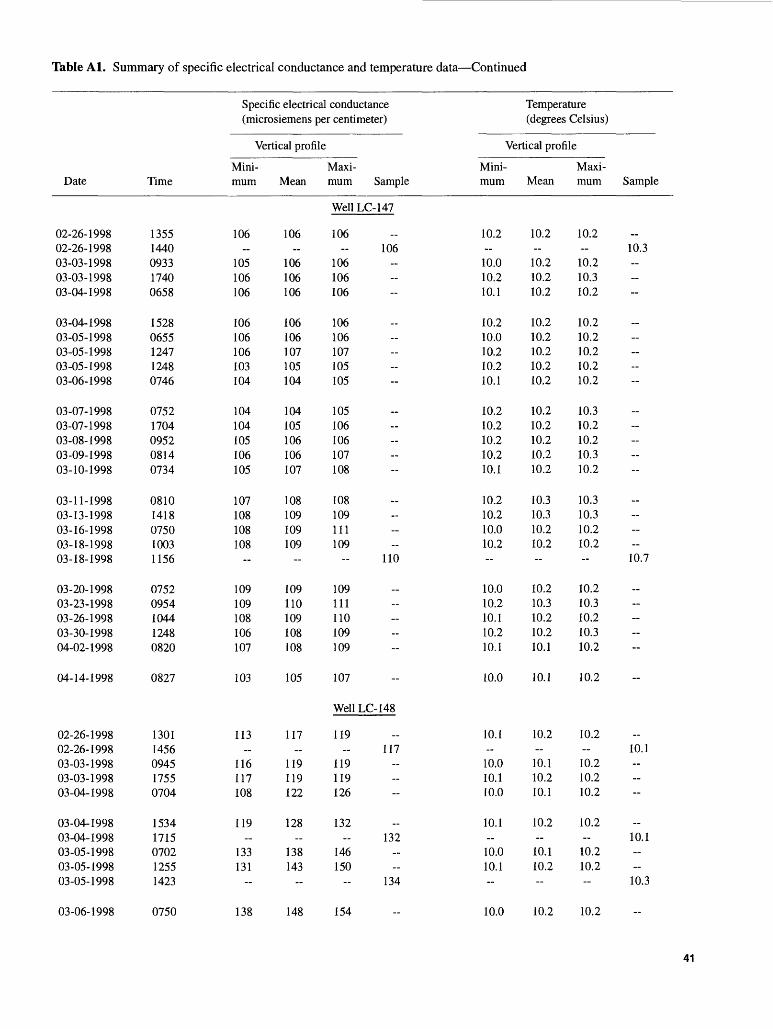
Table Al. Summary of specific electrical conductance and temperature data Continued
Specific electrical conductance (microsiemens per centimeter)
Vertical profile
Date
02-26-199802-26-199803-03-199803-03-199803-04-1998
03-04-199803-05-199803-05-199803-05-199803-06-1998
03-07-199803-07-199803-08-199803-09-199803-10-1998
03-11-199803-13-199803-16-199803-18-199803-18-1998
03-20-199803-23-199803-26-199803-30-199804-02-1998
04-14-1998
02-26-199802-26-199803-03-199803-03-199803-04-1998
03-04-199803-04-199803-05-199803-05-199803-05-1998
Time
13551440093317400658
15280655124712480746
07521704095208140734
08101418075010031156
07520954104412480820
0827
13011456094517550704
15341715070212551423
Mini mum
106
105106106
106106106103104
104104105106105
107108108108
~
109109108106107
103
113~
116117108
119
133131
._
Mean
106
106106106
106106107105104
104105106106107
108109109109-
109110109108108
105
117
119119122
128
138143
._
Maxi mum Sample
Well LC-147
106106
106106106
106106107105105
105106106107108
108109111109
110
109111110109109
107
Well LC-148
119117
119119126
132132
146150
134
Temperature (degrees Celsius)
Vertical profile
Mini mum
10.2
10.010.210.1
10.210.010.210.210.1
10.210.210.210.210.1
10.210.210.010.2-
10.010.210.110.210.1
10.0
10.1
10.010.110.0
10.1 10.010.1
Mean
10.2~
10.210.210.2
10.210.210.210.210.2
10.210.210.210.210.2
10.310.310.210.2-
10.210.310.210.210.1
10.1
10.2-
10.110.210.1
10.2-
10.110.2
Maxi mum
10.2
10.210.310.2
10.210.210.210.210.2
10.310.210.210.310.2
10.310.310.210.2
10.210.310.210.310.2
10.2
10.2-10.210.210.2
10.2
10.210.2
Sample
..10.3 --
_ -
__ -
_.~-~
10.7
----
-
_10.1~ ~
_.10.1~
10.3
03-06-1998 0750 138 148 154 10.0 10.2 10.2
41

Table Al. Summary of specific electrical conductance and temperature data Continued
Specific electrical conductance (microsiemens per centimeter)
Vertical profile
Date TimeMini mum Mean
Maxi mum Sample
Temperature (degrees Celsius)
Vertical profile
Mini mum Mean
Maxi mum Sample
Well LC- 148 Continued
03-06-199803-06-199803-06-199803-06-199803-06-1998
03-06-199803-06-199803-07-199803-07-199803-08-1998
03-09-199803-10-199803-11-199803-13-199803-16-1998
03-18-199803-20-199803-23-199803-26-199803-30-1998
04-02-199804-14-1998
09201144124513421436
15431708080217100958
08280742082213320758
10270802095811141320
08260832
140141143150
143144138133127
118122121116122
121121120118119
116113
148150154155
156157143137130
123123122119122
122122123122122
121116
161160161163
165164148140131
127130124123123
122123124123122
122118
140 --
_ --
_ --
_ --
_-
10.010.110.110.1
10.110.110.110.210.1
10.110.110.110.210.1
10.110.010.210.110.1
10.010.0
10.110.210.210.2
10.210.210.210.210.2
10.210.210.210.310.1
10.210.110.210.210.2
10.110.1
10.110.210.210.2
10.310.210.210.210.2
10.210.210.210.310.2
10.210.210.210.210.2
10.110.1
10.0 ~~~
__- -~
_---~
._~~--
__~
Well LC-149A
02-25-199803-26-1998
16250955 99 100 100
105-
9.5
..9.5
..9.5
9.6-
WellLC-149C
02-25-199802-25-199803-26-1998
161216590959
112
116
114
119
116
121116-
9.3 9.4
9.3 9.5
9.4~9.5
_9.4~
WellLC-149D
02-25-199803-26-1998
16401002 113 114 115
112
..9.4
..9.4
..9.5
9.2
42

Table Al. Summary of specific electrical conductance and temperature data Continued
Specific electrical conductance (microsiemens per centimeter)
Vertical profile
Date
02-27-199802-27-199803-03-199803-04-199803-05-1998
03-06-199803-07-199803-08-199803-09-199803-10-1998
03-10-199803-11-199803-13-199803-16-199803-18-1998
03-20-199803-23-199803-26-199803-30-199804-02-1998
04-06-199804-09-199804-14-1998
02-27-199802-27-199803-03-199803-04-199803-05-1998
03-06-199803-07-199803-08-199803-09-199803-10-1998
03-11-199803-13-199803-16-199803-18-199803-20-1998
Time
15071552171810320736
08510723092807440702
08480729134107250936
07180924092715320758
163607580804
15201625172310350740
08550729093207490715
07371347072809410725
Mini mum
133
132132133
132131131132132
_132132133133
134136133134133
132131128
228
225224222
222221221222220
223224226225230
Mean
133
133133134
132132132132137
_132133134134
134136134135134
136136130
228
226225225
224223223223222
224226227227232
Maxi mum Sample
Well LC- 161
133128
134135151
135135132134173
132134136138137
136137136137135
140147132
Well LC- 162
229239
227226226
227225224225225
224227230230234
Temperature (degrees Celsius)
Vertical profile
Mini mum
9.9 9.79.79.6
9.99.69.99.89.8
_9.89.89.79.8
9.49.89.89.89.6
9.89.69.1
9.7 9.69.79.6
9.69.59.89.7
10.0
9.79.89.49.89.4
Mean
9.9-9.99.99.8
10.09.99.99.99.9
_9.89.89.79.9
9.79.89.89.89.7
9.99.89.4
9.8-9.89.99.8
9.89.89.99.8
10.0
9.89.89.69.89.7
Maxi mum
9.9 9.9
10.010.0
10.19.99.99.9
10.0
_9.9
10.39.99.9
9.89.99.8
10.09.7
10.19.89.5
9.9~9.9
10.09.9
9.99.9
10.09.9
10.2
10.09.99.89.99.8
Sample
..10.6 --
_ ~--
9.9~~--
_- -~
..
_10.1 -
~-~
__-~-
43

Table Al. Summary of specific electrical conductance and temperature data Continued
Specific electrical conductance (microsiemens per centimeter)
Vertical profile
Date
03-23-199803-26-199803-30-199804-02-199804-06-1998
04-09-199804-14-1998
02-26-199802-26-199803-03-199803-03-199803-04-1998
03-04-199803-05-199803-05-199803-06-199803-07-1998
03-07-199803-08-199803-09-199803-09-199803-10-1998
03-11-199803-13-199803-16-199803-18-199803-20-1998
03-23-199803-26-199803-30-199804-02-199804-14-1998
02-27-199803-03-199803-03-199803-04-1998
Time
09280943153808021641
08060808
13551437111817460708
15280706125908000807
17141004083409230747
08301440080210320809
10031117132608300836
1405112517500712
Mini mum
226226226225222
225219
109
109109108
110110109109111
112112112
113
112107112111112
113113111112109
136136134134
Mean
228227227227231
232221
109
Ill111111
111112110112115
116118117
119
117115116114115
115116113114112
137136135135
Maxi mum Sample
Well LC-162
230228228229234
235224
Well LC-26
110111
113113112
113113113115120
123126126
110126
123122120118118
118118116116113
Well LC-26D
138136135135
Temperature (degrees Celsius)
Vertical profile
Mini mum
9.79.69.79.49.9
9.49.3
9.9 9.69.89.5
9.89.69.89.69.6
9.79.89.7 9.7
9.910.09.69.89.6
9.99.99.99.89.6
10.110.110.110.1
Mean
9.89.79.89.69.9
9.79.5
10.0 9.99.99.9
9.99.99.99.99.9
9.99.99.9-9.9
10.010.09.99.99.9
10.010.010.010.09.9
10.110.110.110.1
Maxi mum
9.99.89.99.89.9
9.99.6
10.0
10.010.010.0
10.010.010.110.010.0
10.110.010.1-
10.0
10.110.110.010.010.0
10.010.010.110.010.0
10.110.110.210.1
Sample
.. -
_.--
..10.0--
..
----
-
10.1
_.
"--
---
_
"
44

Table Al. Summary of specific electrical conductance and temperature data Continued
Specific electrical conductance (microsiemens per centimeter)
Vertical profile
Date
03-04-199803-05-199803-05-199803-06-199803-07-1998
03-08-199803-09-199803-10-199803-11-199803-13-1998
03-16-199803-18-199803-20-199803-23-199803-26-1998
03-30-199804-02-199804-14-1998
03-03-199803-04-199803-04-199803-05-199803-05-1998
03-06-199803-07-199803-07-199803-08-199803-09-1998
03-10-199803-11-199803-13-199803-16-199803-18-1998
03-20-199803-23-199803-26-199804-02-1998
Time
15400708130208040816
10060840075108371446
08061038081410061120
133208340840
09100842160106351333
06550738144909430758
07220745135507390948
0733094410260809
Mini mum
134134134133133
133133133133136
136137138139139
136138133
.. -
_-- ~
_ -~
_ -
Mean
135135135133134
134134134134136
137137139140140
137138134
120*196!203
H92-
!200206216192125
122125124126127
128128128127
Maxi mum Sample
Well LC-26D
135136136134134
135134134136137
138139140140141
137139135
WellLR-1
..
*203
..
.. ..-
_-. -
.. ..
Temperature (degrees Celsius)
Vertical profile
Mini mum
10.110.110.110.110.2
10.110.110.110.110.1
10.110.110.110.210.0
10.110.110.1
.. ~
_ -
_ -
..
Mean
10.110.110.110.110.2
10.110.110.110.210.1
10.110.110.110.210.1
10.110.110.1
10.09.2
10.09.0-
9.59.9
10.210.110.1
10.110.210.310.010.1
9.810.310.19.9
Maxi mum Sample
10.210.110.210.110.2
10.210.110.110.210.1
10.110.210.110.210.2
10.210.210.1
_....
9.9
_._ -
_ --
__..._.
45

Table Al. Summary of specific electrical conductance and temperature data Continued
Specific electrical conductance (microsiemens per centimeter)
Vertical profile
Date TimeMini mum Mean
Maxi mum Sample
Temperature (degrees Celsius)
Vertical profile
Mini mum Mean
Maxi mum Sample
Well LR-2
02-26-199802-26-199803-03-199803-03-199803-04-1998
03-04-199803-05-199803-05-199803-06-199803-06-1998
03-07-199803-07-199803-07-199803-07-199803-08-1998
03-09-199803-10-199803-11-199803-13-199803-13-1998
03-16-199803-16-199803-16-199803-18-199803-20-1998
03-23-199803-26-199803-30-199804-02-199804-14-1998
15491657094017530700
15310658125107490751
07550759100017050956
08240738081514221730
07540921093910080757
09561047131408240827
104
104105105
111111104104105
103104
141131
134126125121123
122120
117115
116114112112105
119
127125124
129129128135137
143143
153155
158156152143142
138135
136132
133132129129124
125
155148147
160147146146146
153155
157158
164164162167148
158149
159159
161168160162160
104 -~
_ -
_
144 -
_ -
_
136 -
_ -
10.2
10.110.210.2
10.210.210.210.210.2
10.210.2
10.210.2
10.210.210.210.210.2
10.110.1 10.110.1
10.210.210.210.210.1
10.2
10.210.210.2
10.210.210.210.210.2
10.210.2
10.210.2
10.310.210.310.210.2
10.210.2 10.210.2
10.210.210.210.210.2
10.2
10.210.310.2
10.310.210.310.210.2
10.310.3
10.310.2
10.310.210.310.210.4
10.210.2 10.310.2
10.310.210.210.210.2
..10.3 -
_ -
_
10.1 ~
_ ~
_
10.4-
_ -~
East Gate Pump-and-Treat Effluent
02-25-199802-26-199802-27-199803-04-199803-04-1998
03-06-199803-07-199803-07-1998
15050745165506101138
083507111637
-
..
-
.. _-
-
..
123141123135131
126124129
.. -
_
.. -
_
..~ -
_
10.89.7
10.012.5
9.69.4
10.7
46

Table Al. Summary of specific electrical conductance and temperature data Continued
Specific electrical conductance Temperature (microsiemens per centimeter) (degrees Celsius)
Vertical profile Vertical profile
Mini- Maxi- Mini- Maxi- Date Time mum Mean mum Sample mum Mean mum Sample
East Gate Pump-and-Treat Effluent Continued
03-08-199803-09-199803-10-199803-11-199803-13-1998
03-16-199803-18-199803-20-199803-23-199803-26-1998
04-02-199804-06-199804-09-199804-14-199804-14-1998
09190735064507171535
07150927071209170928
07401618074607581006
122125122127124
126128126126128
126129121119123
10.511.010.810.811.0
10.811.110.410.910.3
10.811.211.210.610.7
losing with sodium chloride temporarily stopped for collection of sample.
47

48
80
60
UJ O
guj 40
O 01
OCO 20 LU Z
UJ^O LULL CO00LU DCQ. OCO ^ 0CO -7CO ^LUOXLU
-20
-40
r^ "*
&
-10 0 10 20 30 40
BROMIDE CONCENTRATION, IN MILLIGRAMS PER LITER
Figure A1 . Excess specific electrical conductance as a function of bromide concentration in samples.
50
ft U.S. GOVERNMENT PRINTING OFFICE: 1999 589-121 / 03005 Region No. 10

E.A. Prych A
Tracer Test to Estim
ate Hydraulic C
onductivities and Dispersivities of S
ediments in the S
hallow A
quifer at the East Gate D
isposal Yard, Fort Lewis, W
ashington U
SGS-W
RIR
99-4244