A Toolbox of Query Evaluation Techniques for Probabilistic Databases
55
2nd Workshop on Management and mining Of UNcertain Data (MOUND) Long Beach, March 1st, 2010 A Toolbox of Query Evaluation Techniques for Probabilistic Databases Dan Olteanu, Oxford University Computing Laboratory
Transcript of A Toolbox of Query Evaluation Techniques for Probabilistic Databases

2nd Workshop on Management and mining Of UNcertain Data (MOUND)Long Beach, March 1st, 2010
A Toolbox of Query Evaluation Techniques forProbabilistic Databases
Dan Olteanu, Oxford University Computing Laboratory

Uncertain and Probabilistic Data
Uncertain and probabilistic data is commonplace:
(Web) information extraction
Processing manually entered data (such as census forms)
Data integration, data cleaning
Risk management: Decision support queries, hypothetical queries
Social network analysis
Managing scientific data; sensor data
Crime fighting, surveillance, plagiarism detection, predicting terrorist actions
Relational DBMSs are not flexible enough to accommodate such data
one tries to find a “good” yet partial fit of the data in the relational format
Recent years have seen advances in developing
representation models for uncertain/probabilistic data,
uncertainty-aware query languages, and
scalable query evaluation techniques for such data.

Probabilistic Databases Today
Many active projects, for instance
Mystiq, Lahar (Washington U.)
Trio (Stanford)
MCDB (IBM Almaden & Florida)
BayesStore (Berkeley)
Orion (Purdue)
PrDB (Maryland)
Also at UMass, Waterloo, Hong Kong, Florida State, Wisconsin, MIT, . . .
Projects I am involved in
MayBMS (Cornell+Oxford)
◮ Uncertainty-aware query languages and data representation models
SPROUT = Scalable Query PROcessing on Uncertain Tables (Oxford)◮ Query engine that extends PostgreSQL backend
MayBMS and SPROUT are available at maybms.sourceforge.net.

Outline of this talk
Two (discrete) probabilistic data models◮ U-relational databases: a complete but “hard” model◮ Tuple-independent databases: a restricted but “easier” model
Query evaluation in probabilistic databases◮ The non-probabilistic case◮ Data complexity in the probabilistic case
Exact query evaluation techniques◮ Evaluation of tractable conjunctive queries
⋆ using OBDDs (ordered binary decision diagrams)⋆ using relational plans
◮ Detection of large tractable query & data sub-instances
Approximate query evaluation techniques with error guarantees◮ Monte Carlo techniques (FPRAS)◮ Incremental evaluation techniques based on lineage factorization

U-relational Probabilistic Databases
Syntax.Probabilistic databases are relational databases where
There is a finite set of independent random variables X = {x1, . . . , xn} withfinite domains Domx1 , . . . ,Domxn .
Tuples are associated with lineage, i.e., conjunctions of atomic events of theform xi = a or xi 6= a where xi ∈ X and a ∈ Domxi .
There is a probability distribution over the assignments of each variable.
Semantics.
Possible worlds defined by total assignments θ over X.
The world defined by assignment θ◮ consists of all tuples with condition φ such that θ(φ) = true.◮ has probability defined by the product of probabilities of each assignment in θ.
This formalism can represent any discrete probability distribution over relational databases.

Example: Probabilistic Databases
Consider a simplified TPC-H scenario with customers (Cust) and orders (Ord):
Custckey cname V1 P1 V2 P2
1 Joe x1 0.1 x3 0.12 Dan x1 0.9 x4 0.53 Li x2 0.3 x4 0.54 Mo x2 0.7 x5 0.2
Ordokey ckey odate V1 P1 V2 P2
1 1 1995-01-10 y1 0.1 x5 0.22 1 1996-01-09 y2 0.2 x4 0.53 2 1994-11-11 y3 0.3 x3 0.1
Variables are Boolean (wlog); write x instead of x = 1, x instead of x = 0.
A pair (Vi ,Pi ) states that the variable assignment given by Vi has theprobability given by Pi .
Lineage can represent arbitrary correlations between tuples, eg,
◮ (1,Joe) and (3,Li) are independent: They use disjoint sets of variables.◮ (1,Joe) and (2,Dan) are mutually exclusive: x1 is either true or false.

Example: Probabilistic Databases
Consider the world A defined by a total assignment θ:
x1, x2, y1, y2 are true, and all other variables are false.
Custckey cname V1 P1 V2 P2
1 Joe x1 0.1 x3 0.12 Dan x1 0.9 x4 0.53 Li x2 0.3 x4 0.54 Mo x2 0.7 x5 0.2
Ordokey ckey odate V1 P1 V2 P2
1 1 1995-01-10 y1 0.1 x5 0.22 1 1996-01-09 y2 0.2 x4 0.53 2 1994-11-11 y3 0.3 x3 0.1
The world A is as follows:
Custckey cname3 Li
Ordokey ckey odate1 1 1995-01-102 1 1996-01-09
Probability of A = product of probabilities of the assignments in θ:
Pr(A) = Pr(θ) = Pr(x1) · Pr(x2) · Pr(y1) · Pr(y2) · Pr(x3) · Pr(x4) · Pr(x5) · Pr(y3).

Tuple-independent Probabilistic Databases
Tuple-independent: Tuples have independent lineage, or equivalently
Each tuple t is associated with a Boolean random variable xt .
Tuple t is in the world defined by θ if xt = true holds in θ.
Custckey cname V P1 Joe x1 0.12 Dan x2 0.23 Li x3 0.34 Mo x4 0.4
Ordokey ckey odate V P1 1 1995-01-10 y1 0.12 1 1996-01-09 y2 0.23 2 1994-11-11 y3 0.34 2 1993-01-08 y4 0.45 3 1995-08-15 y5 0.56 3 1996-12-25 y6 0.6
Itemokey disc ckey V P1 0.1 1 z1 0.11 0.2 1 z2 0.23 0.4 2 z3 0.33 0.1 2 z4 0.44 0.4 2 z5 0.55 0.1 3 z6 0.6

Query Evaluation in Probabilistic Databases
Subsumed by general probabilistic inference, which was investigated in AI formany years. Is there something left to do for the database community?

Query Evaluation in Probabilistic Databases
Subsumed by general probabilistic inference, which was investigated in AI formany years. Is there something left to do for the database community?
The database approach is based on two fundamental observations:
the separation of (very large) data and (small and fixed) query, and
the use of mature relational query engines to achieve scalability.

Query Evaluation in Probabilistic Databases
The MayBMS/SPROUT approach:
Given probabilistic database T = {A1, . . . ,An} and query q.
Under possible world semantics: q is evaluated in each possible world of T .
Is there q such that q(T ) = {q(A1), . . . , q(An)}? [Imielinski&Lipski84]
T q(T )
{A1, . . . ,An} {q(A1), . . . , q(An)}
rep
q
q
rep
Compute the probability of each distinct tuple in q(T ).
How hard is query evaluation in probabilistic databases?
q(T ) can be computed in PTIME (wrt data complexity) for relational algebraqueries and U-relational databases [AJK&O.08]
Probability computation is in general very hard, but there are tractable cases

Example: Query Evaluation
Query asking for the dates of discounted orders shipped to customer ’Joe’:
Q(odate) :- Cust(ckey ,′ Joe′),Ord(okey , ckey , odate), Item(okey , disc, ckey), disc > 0odate Vc Pc Vo Po Vi Pi tuple probability
1995-01-10 x1 0.1 y1 0.1 z1 0.1 0.1 · 0.1 · 0.11995-01-10 x1 0.1 y1 0.1 z2 0.2 0.1 · 0.1 · 0.2
Query Q is Q changed so that the lineage of input tuples is copied in theanswer tuples.
Probability of distinct answer tuple (1995-01-10) is the probability of theassociated lineage x1y1z1 + x1y1z2.
Difficulty:
The sets of satisfying assigments of any two clauses may overlap.
It may require to iterate over its (exponentially many) satisfying assignments.

Dichotomy Property
Discussed here [Dalvi&Suciu07]:
Conjunctive queries without self-joins (CQ1) on
Tuple-independent databases.
The data complexity of any CQ1 query is either FP or #P-hard.
#P = class of functions f (x) for which there exists a PTIMEnon-deterministic Turing machine M such that f (x) = number of acceptingcomputations of M on input x .
FP = class of functions that can be solved by a deterministic Turing machinein PTIME. These functions can have any output, not only true/false.
Further tractability results not discussed here:
Dichotomy for conjunctive queries with self-joins [Dalvi&Suciu07b]
Tractable queries with inequalities (<,≤, 6=) [O.&Huang08,O.&Huang09]
Extension to the block-independent disjoint model follow easily [DRS07]

All tractable CQ1 queries are hierarchical
A query is hierarchical if for any two non-head variables, either their sets ofsubgoals are disjoint, or one set is contained in the other.
Q(odate) :- Cust(ckey ,′ Joe′),Ord(okey , ckey , odate), Item(okey , disc, ckey), disc > 0.
is hierarchical; also without odate as head variable.
subgoals(disc)={Item}, subgoals(okey)={Ord, Item}, subgoals(ckey)={Cust,Ord, Item}.
It holds that subgoals(disc)⊆ subgoals(okey)⊆ subgoals(ckey).
ckey
ckey,okey
Ord(okey,ckey,odate) Item(okey,disc,ckey)
Cust(ckey,’Joe’)

Exact Query Evaluation

Exact Query Evaluation using SPROUT
Cast the query evaluation problem as a decision diagram construction problem.
Given a query q and a probabilistic database D,each distinct tuple t ∈ q(D) is associated with a DNF expression φt .
Probability of t is probability of φt .
Compile φt into an equivalent binary decision diagram (BDD).
Probability of φt is then the probability of its BDD.
SPROUT employs secondary-storage techniques for BDD construction andprobability computation.

BDDs
Commonly used to represent compactly large Boolean expressions.
Idea: Decompose Boolean expressions using variable elimination and avoidredundancy in the representation.Variable elimination by Shannon’s expansion: φ = x · φ |x +x · φ |x .
Supports linear-time probability computation.
Pr(φ) = Pr(x · φ |x +x · φ |x)
= Pr(x · φ |x) + Pr(x · φ |x)
= Pr(x) · Pr(φ |x) + Pr(x) · Pr(φ |x)
Ordered BDDs (OBDDs):
Variable order π = order of variable eliminations;the same variable order on all root-to-leaf paths ⇒ ordered BDDs (OBDDs)
An OBDD for φ is uniquely identified by the pair (φ, π).
Compilation example
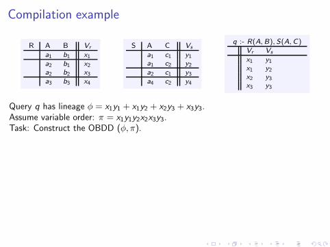
R A B Vr
a1 b1 x1a2 b1 x2a2 b2 x3a3 b3 x4
S A C Vs
a1 c1 y1a1 c2 y2a2 c1 y3a4 c2 y4
q :- R(A,B), S(A,C)Vr Vs
x1 y1x1 y2x2 y3x3 y3
Query q has lineage φ = x1y1 + x1y2 + x2y3 + x3y3.Assume variable order: π = x1y1y2x2x3y3.Task: Construct the OBDD (φ, π).

Compilation example
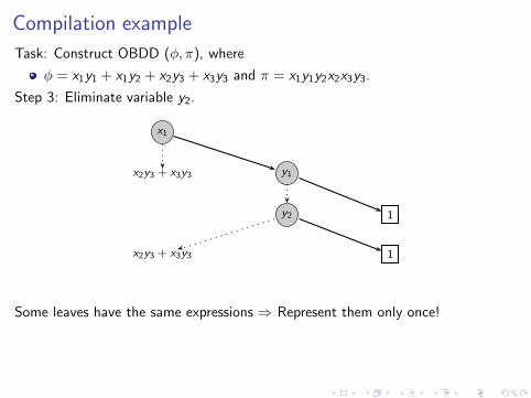
Task: Construct OBDD (φ, π), where
φ = x1y1 + x1y2 + x2y3 + x3y3 and π = x1y1y2x2x3y3.
Step 1: Eliminate variable x1 in φ.
x1
x2y3 + x3y3 y1 + y2 + x2y3 + x3y3

Compilation example
Task: Construct OBDD (φ, π), where
φ = x1y1 + x1y2 + x2y3 + x3y3 and π = x1y1y2x2x3y3.
Step 2: Eliminate variable y1.
x1
x2y3 + x3y3 y1
y2 + x2y3 + x3y3 1
Compilation example
Task: Construct OBDD (φ, π), where
φ = x1y1 + x1y2 + x2y3 + x3y3 and π = x1y1y2x2x3y3.
Step 3: Eliminate variable y2.
x1
x2y3 + x3y3 y1
y2 1
x2y3 + x3y3 1
Some leaves have the same expressions ⇒ Represent them only once!

Compilation example
Task: Construct OBDD (φ, π), where
φ = x1y1 + x1y2 + x2y3 + x3y3 and π = x1y1y2x2x3y3.
Step 4: Merge leaves with the same expressions.
x1
y1
y2
x2y3 + x3y3 1

Compilation example
Task: Construct OBDD (φ, π), where
φ = x1y1 + x1y2 + x2y3 + x3y3 and π = x1y1y2x2x3y3.
Step 5: Eliminate variable x2.
x1
y1
y2
x2 1
x3y3 y3 + x3y3

Compilation example
Task: Construct OBDD (φ, π), where
φ = x1y1 + x1y2 + x2y3 + x3y3 and π = x1y1y2x2x3y3.
Step 6: Replace y3 + x3y3 by y3.
x1
y1
y2
x2 1
x3y3 y3

Compilation example
Task: Construct OBDD (φ, π), where
φ = x1y1 + x1y2 + x2y3 + x3y3 and π = x1y1y2x2x3y3.
Step 7: Eliminate variable x3.
x1
y1
y2
x2 1
x3 y3
0 y3
Compilation example
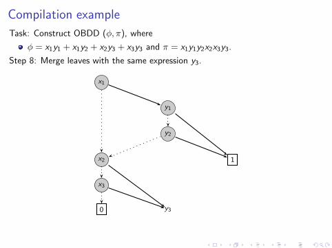
Task: Construct OBDD (φ, π), where
φ = x1y1 + x1y2 + x2y3 + x3y3 and π = x1y1y2x2x3y3.
Step 8: Merge leaves with the same expression y3.
x1
y1
y2
x2 1
x3
0 y3
Compilation example
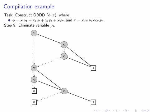
Task: Construct OBDD (φ, π), where
φ = x1y1 + x1y2 + x2y3 + x3y3 and π = x1y1y2x2x3y3.Step 9: Eliminate variable y3.
x1
y1
y2
x2 1
x3
0 y3
0 1

Compilation example
Task: Construct OBDD (φ, π), where
φ = x1y1 + x1y2 + x2y3 + x3y3 and π = x1y1y2x2x3y3.Step 10 (final): Merge leaves with the same expression (0 or 1).
x1
y1
y2
x2
x3
y3
0 1

Compilation example: Summing Up
OBDD (φ, π) has size bounded in the number of literals in φ.(exactly one node per variable in φ in our example)
Questions
1 Is this property shared by the BDDs of many queries?
2 Can we efficiently construct such succinct BDDs?

Compilation example: Summing Up
OBDD (φ, π) has size bounded in the number of literals in φ.(exactly one node per variable in φ in our example)
Questions
1 Is this property shared by the BDDs of many queries?
2 Can we efficiently construct such succinct BDDs?
The answer is in the affirmative for both questions!

Tractable Queries and Succinct BDDs
For any hierarchical query q and database D, ∀t ∈ q(D), and lineage φt ,
There is a variable order π computable in time O(|φt | · log2 |φt |) such that
The OBDD (φt , π) has size O(|Vars(φt )) and can be computed in timeO(|φt | · log |φt |).
φt can be factorized into read-once functions! [O.&Huang08]
BDD construction in polynomial time for a class of tractable conjunctive querieswith inequalities. [O.&Huang09]
Good variable orders can be statically derived from the query structure!

Static Query Analysis: Query Signatures
Query signatures for TQ queries capture
the structures of queries and
the one/many-to-one/many relationships between the query tables;
variable orders for succinct BDDs representing compiled lineage!
A
R(A,B) S(A,C)
Query q :- R(A,B), S(A,C ) has signature (R∗S∗)∗ .
There may be several R-tuples with the same A-value, hence R∗
There may be several S-tuples with the same A-value, hence S∗
R and S join on A, hence R∗S∗
There may be several A-values in R and S , hence (R∗S∗)∗
Variable orders captured by (R∗S∗)∗ (xi ’s are from R , yj ’s are from S):
{[x1(y1y2)][(x2x3)y3]}, {[(x2x3)y3][x1(y1y2)]}, {[y3(x3x2)][x1(y2y1)]}, etc.

Query Rewriting under Functional Dependencies (FDs)
FDs on tuple-independent databases can help deriving better query signatures.
Given a set of FDs Σ and a conjunctive query of the form
Q = πA0(σφ(R1(A1) ⊲⊳ . . . ⊲⊳ Rn(An))
where φ is a conjunction of unary predicates. Let Σ0 = CLOSUREΣ(A0).Then, the Boolean query
π∅(σφ(R1(CLOSUREΣ(A1)− Σ0) ⊲⊳ . . . ⊲⊳ Rn(CLOSUREΣ(An)− Σ0)))
is called the FD-reduct of Q under Σ. [O.&HK09]
If there is a sequence of chase steps under Σ that turns Q into a hierarchicalquery, then the fixpoint of the chase (the FD-reduct) is hierarchical.
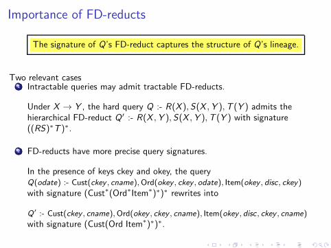
Importance of FD-reducts
The signature of Q’s FD-reduct captures the structure of Q’s lineage.
Two relevant cases1 Intractable queries may admit tractable FD-reducts.
Under X → Y , the hard query Q :- R(X ), S(X ,Y ),T (Y ) admits thehierarchical FD-reduct Q ′ :- R(X ,Y ), S(X ,Y ),T (Y ) with signature((RS)∗T )∗.
2 FD-reducts have more precise query signatures.
In the presence of keys ckey and okey, the queryQ(odate) :- Cust(ckey , cname),Ord(okey , ckey , odate), Item(okey , disc, ckey)
with signature (Cust∗(Ord∗Item∗)∗)∗ rewrites into
Q ′ :- Cust(ckey , cname),Ord(okey , ckey , cname), Item(okey , disc, ckey , cname)
with signature (Cust(Ord Item∗)∗)∗.

Case Study: TPC-H Queries
Considered the conjunctive part of each of the 22 TPC-H queries
Boolean versions (B)
with original selection attributes, but without aggregates (O)
Hierarchical in the absence of key constraints
8 queries (B)
13 queries (O)
Hierarchical in the presence of key constraints
8+4 queries (B)
13+4 queries (O)
In-depth study athttp://www.comlab.ox.ac.uk/people/dan.olteanu/papers/icde09queries.html
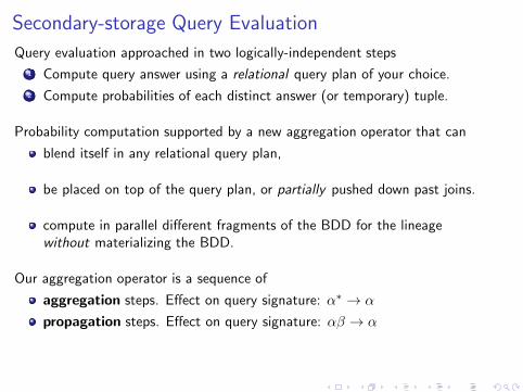
Secondary-storage Query Evaluation
Query evaluation approached in two logically-independent steps
1 Compute query answer using a relational query plan of your choice.
2 Compute probabilities of each distinct answer (or temporary) tuple.
Probability computation supported by a new aggregation operator that can
blend itself in any relational query plan,
be placed on top of the query plan, or partially pushed down past joins.
compute in parallel different fragments of the BDD for the lineagewithout materializing the BDD.
Our aggregation operator is a sequence of
aggregation steps. Effect on query signature: α∗ → α
propagation steps. Effect on query signature: αβ → α

Example of Probability Computationx1
y1
y2
x2
x3
y3
0 1
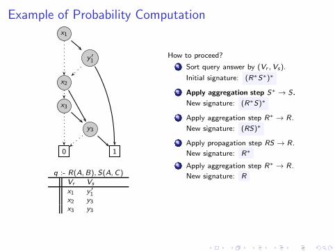
q :- R(A,B), S(A,C)Vr Vs
x1 y1x1 y2x2 y3x3 y3
How to proceed?
1 Sort query answer by (Vr ,Vs).
Initial signature: (R∗S∗)∗
2 Apply aggregation step S∗→ S.
New signature: (R∗S)∗
3 Apply aggregation step R∗→ R.
New signature: (RS)∗
4 Apply propagation step RS → R.
New signature: R∗
5 Apply aggregation step R∗→ R.
New signature: R

Example of Probability Computationx1
y1
y2
x2
x3
y3
0 1
q :- R(A,B), S(A,C)Vr Vs
x1 y1 + y2x2 y3x3 y3
How to proceed?
1 Sort query answer by (Vr ,Vs).
Initial signature: (R∗S∗)∗
2 Apply aggregation step S∗→ S.
New signature: (R∗S)∗
3 Apply aggregation step R∗→ R.
New signature: (RS)∗
4 Apply propagation step RS → R.
New signature: R∗
5 Apply aggregation step R∗→ R.
New signature: R
Example of Probability Computationx1
y ′
1
x2
x3
y3
0 1
q :- R(A,B), S(A,C)Vr Vs
x1 y ′
1x2 y3x3 y3
How to proceed?
1 Sort query answer by (Vr ,Vs).
Initial signature: (R∗S∗)∗
2 Apply aggregation step S∗→ S.
New signature: (R∗S)∗
3 Apply aggregation step R∗→ R.
New signature: (RS)∗
4 Apply propagation step RS → R.
New signature: R∗
5 Apply aggregation step R∗→ R.
New signature: R

Example of Probability Computationx1
y ′
1
x2
x3
y3
0 1
q :- R(A,B), S(A,C)Vr Vs
x1 y ′
1x2 + x3 y3
How to proceed?
1 Sort query answer by (Vr ,Vs).
Initial signature: (R∗S∗)∗
2 Apply aggregation step S∗→ S.
New signature: (R∗S)∗
3 Apply aggregation step R∗→ R.
New signature: (RS)∗
4 Apply propagation step RS → R.
New signature: R∗
5 Apply aggregation step R∗→ R.
New signature: R

Example of Probability Computationx1
y ′
1
x ′2
y3
0 1
q :- R(A,B), S(A,C)Vr Vs
x1 y ′
1x ′2 y3
How to proceed?
1 Sort query answer by (Vr ,Vs).
Initial signature: (R∗S∗)∗
2 Apply aggregation step S∗→ S.
New signature: (R∗S)∗
3 Apply aggregation step R∗→ R.
New signature: (RS)∗
4 Apply propagation step RS → R.
New signature: R∗
5 Apply aggregation step R∗→ R.
New signature: R

Example of Probability Computationx1
y ′
1
x ′2
y3
0 1
q :- R(A,B), S(A,C)Vr
x1y′
1x ′2y3
How to proceed?
1 Sort query answer by (Vr ,Vs).
Initial signature: (R∗S∗)∗
2 Apply aggregation step S∗→ S.
New signature: (R∗S)∗
3 Apply aggregation step R∗→ R.
New signature: (RS)∗
4 Apply propagation step RS → R.
New signature: R∗
5 Apply aggregation step R∗→ R.
New signature: R

Example of Probability Computation
x ′′1
x ′′2
0 1
q :- R(A,B), S(A,C)Vr
x ′′1x ′′2
How to proceed?
1 Sort query answer by (Vr ,Vs).
Initial signature: (R∗S∗)∗
2 Apply aggregation step S∗→ S.
New signature: (R∗S)∗
3 Apply aggregation step R∗→ R.
New signature: (RS)∗
4 Apply propagation step RS → R.
New signature: R∗
5 Apply aggregation step R∗→ R.
New signature: R

Example of Probability Computation
x ′′1
x ′′2
0 1
q :- R(A,B), S(A,C)Vr
x ′′1 + x ′′2
How to proceed?
1 Sort query answer by (Vr ,Vs).
Initial signature: (R∗S∗)∗
2 Apply aggregation step S∗→ S.
New signature: (R∗S)∗
3 Apply aggregation step R∗→ R.
New signature: (RS)∗
4 Apply propagation step RS → R.
New signature: R∗
5 Apply aggregation step R∗→ R.
New signature: R

Example of Probability Computation
x ′′′
0 1
q :- R(A,B), S(A,C)Vr
x ′′′
Return the probability of x ′′′.
How to proceed?
1 Sort query answer by (Vr ,Vs).
Initial signature: (R∗S∗)∗
2 Apply aggregation step S∗→ S.
New signature: (R∗S)∗
3 Apply aggregation step R∗→ R.
New signature: (RS)∗
4 Apply propagation step RS → R.
New signature: R∗
5 Apply aggregation step R∗→ R.
New signature: R
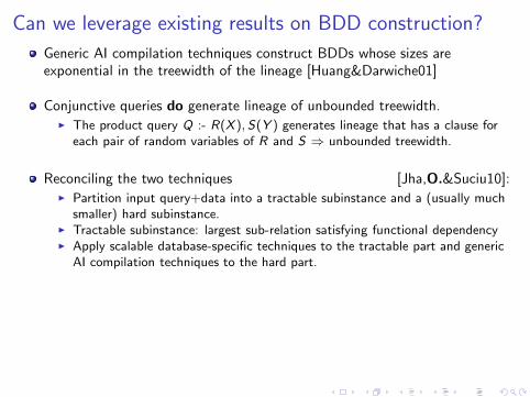
Can we leverage existing results on BDD construction?
Generic AI compilation techniques construct BDDs whose sizes areexponential in the treewidth of the lineage [Huang&Darwiche01]
Conjunctive queries do generate lineage of unbounded treewidth.◮ The product query Q :- R(X ),S(Y ) generates lineage that has a clause for
each pair of random variables of R and S ⇒ unbounded treewidth.
Reconciling the two techniques [Jha,O.&Suciu10]:◮ Partition input query+data into a tractable subinstance and a (usually much
smaller) hard subinstance.◮ Tractable subinstance: largest sub-relation satisfying functional dependency◮ Apply scalable database-specific techniques to the tractable part and generic
AI compilation techniques to the hard part.

Query Optimization: Types of Query Plans
Our previous examples considered lazy plans, where
probability computation done after the computation of answer tuples
unrestricted search space for good query plans
especially desirable when join conditions are selective (eg, TPC-H)!
(Cust∗(Ord∗Item∗)∗)∗
πodate
1ckey,okey
1ckey
σcname=′Joe′
Cust
Ord
σdisc>0
Item
BUT, we can push down probability computation!
Query Optimization: Types of Query Plans
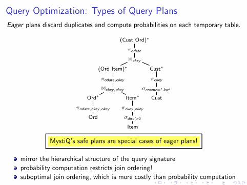
Eager plans discard duplicates and compute probabilities on each temporary table.
(Cust Ord)∗
πodate
1ckey
(Ord Item)∗
πodate,ckey
1ckey,okey
Ord∗
πodate,ckey,okey
Ord
Item∗
πckey,okey
σdisc>0
Item
Cust∗
πckey
σcname=′Joe′
Cust
MystiQ’s safe plans are special cases of eager plans!
mirror the hierarchical structure of the query signature
probability computation restricts join ordering!
suboptimal join ordering, which is more costly than probability computation

Approximate Query Evaluation

Approximate Query Evaluation using Monte Carlo
Using Karp-Luby FPRAS [Karp&Luby83], [Graedel&Gurevitch&Hirsch98]
Input: Boolean formula in DNF φ = C1 + · · ·+ Cm with variables V (φ)
Cnt ← 0; S ← Pr(C1) + · · ·+ Pr(Cm)
repeat N times
randomly choose 1 ≤ i ≤ m with probability Pr(Ci )/S
randomly choose a total valuation λ over V (φ) such that λ(Ci ) = true
if ∀1 ≤ j < i : λ(Cj) = false then Cnt = Cnt + 1
P = Cnt/N × S/2|V (φ)|
return P/* ≈ Pr(φ)*/
If N ≥ (1/m)× (4 ln(2/δ)/ǫ2) then Pr [| P/Pr(φ)− 1 |> ǫ] < δ.
Slightly modified algorithms are used in MayBMS, MystiQ, and MCDB.
Veeeery sloooow in practice: SPROUT query plans are about two orders ofmagnitude faster that the optimized Monte Carlo.

Approximate Evaluation with SPROUT
Monte Carlo simulations are very powerful and generic
◮ only require sampling the formula, no knowledge of its structure
Why not exploit the structure of the input formula? [O.&HK10]
◮ incrementally compile it into an equivalent decomposed form that allows forefficient probability computation
◮ in practice, good approximations are obtained after a few decomposition steps◮ Topic of my ICDE10 talk tomorrow :-)

Thanks!

Literature on Probabilistic Relational Data
Antova, Jansen, Koch, Olteanu. Fast and Simple Relational Processing of
Uncertain Data. ICDE 2008.
Dalvi, Suciu Efficient Query Evaluation on Probabilistic Databases. VLDBJ 2007.
Dalvi, Suciu. The Dichotomy of Conjunctive Queries on Probabilistic Structures.PODS 2007.
Dalvi, Suciu. Management of Probabilistic Data: Foundations and Challenges.PODS 2007.
Karp, Luby, Madras. Monte-Carlo Approximation Algorithms for Enumeration
Problems. J. Algorithms 1989.
Olteanu, Huang. Using OBDDs for Efficient Query Evaluation on Probabilistic
Databases. SUM 2008.

Literature on Probabilistic Relational Data
Olteanu, Huang. Secondary-Storage Confidence Computation for Conjunctive
Queries with Inequalities. SIGMOD 2009.
Olteanu, Huang, Koch. SPROUT: Lazy vs. Eager Query Plans for
Tuple-Independent Probabilistic Databases. ICDE 2009.
Olteanu, Huang, Koch. Approximate Confidence Computation in Probabilistic
Databases. ICDE 2010.
Re, Dalvi, Suciu. Efficient Top-k Query Evaluation on Probabilistic Data. ICDE2007.
Sen, Deshpande. Representing and Querying Correlated Tuples in Probabilistic
Databases. ICDE 2007.
Valiant. The Complexity of Enumeration and Reliability Problems. SIAM J.Comput. 1979.


![Archimedes: Efficient Query Processing over Probabilistic ...edge from existing KBs [5], query-driven inference to compute probabilities of the query facts [35], and the UDA-GISTframeworkforin-databasedata-paralleland](https://static.fdocuments.in/doc/165x107/5f48edeb5760ae07f21c4770/archimedes-eficient-query-processing-over-probabilistic-edge-from-existing.jpg)