A Time-Parallel Implicit Method for Accelerating the...

INTERNATIONAL JOURNAL FOR NUMERICAL METHODS IN ENGINEERINGInt. J. Numer. Meth. Engng 2008; 0:1–25 Prepared using nmeauth.cls [Version: 2000/01/19 v2.0]

A Time-Parallel Implicit Method for Accelerating the Solution ofNonlinear Structural Dynamics Problems

Julien Cortial1 and Charbel Farhat2∗

1 Institute for Computational and Mathematical Engineering2 Department of Mechanical Engineering and Institute for Computational and Mathematical Engineering

Stanford University, Mail Code 3035, Stanford, CA 94305, U.S.A.

SUMMARY

The Parallel Implicit Time-integration Algorithm (PITA) is among a very limited number of time-integrators that have been successfully applied to the time-parallel solution of linear second-orderhyperbolic problems such as those encountered in structural dynamics. Time-parallelism can be ofparamount importance to fast computations, for example, when space-parallelism is unfeasible as inproblems with a relatively small number of degrees of freedom in general, and reduced-order modelapplications in particular, or when reaching the fastest possible CPU time is desired and requires theexploitation of both space- and time-parallelisms. This paper extends the previously developed PITAto the nonlinear case. It also demonstrates its application to the reduction of the time-to-solution ona Linux cluster of sample nonlinear structural dynamics problems. Copyright c© 2008 John Wiley &Sons, Ltd.

key words: nonlinear dynamics, parallel computing, PITA, time-integration, time-parallel

1. INTRODUCTION

The parallelization of the time-loop of a partial differential equation solver, or time-parallelism,has in general received little attention in the literature compared to the parallelization of itsspace-loop. This is because time-parallelism — where the solution is computed simultaneouslyat different time-instances — is harder to achieve efficiently than space-parallelism, due tothe inherently sequential nature of the time-integration process. However, time-parallelismcan be of paramount importance to many applications. These include those time-dependentproblems where the underlying computational models have either very few spatial degrees offreedom (dof) to enable any significant amount of space-parallelism, or not enough spatial dofto efficiently exploit a given large number of processors. Problems in robotics and proteinfolding, and more generally, time-dependent problems arising from reduced-order models

Contract/grant sponsor: National Science Foundation; contract/grant number: 0540419∗Correspondence to: Department of Mechanical Engineering, Stanford University, Mail Code 3035, Stanford,CA 94305, U.S.A.

Received 0Copyright c© 2008 John Wiley & Sons, Ltd. Revised 0

Accepted 0

2 J. CORTIAL AND C. FARHAT

usually fall in the first category. Many structural dynamics problems, even those with hundredsof thousands of dof, can fall in the second category when massively parallel computations aredesired. Accelerating the time-to-solution of the first category of problems is crucial for real-time or near-real-time applications, and time-parallelism can be a key factor for achievingthis objective. With the advent of massively parallel systems with thousands of cores, time-parallelism also provides a venue for reducing the time-to-solution of fixed size problems of thesecond category below the minimum attainable using space-parallelism alone on such systems.

Various methods based on waveform relaxation [1, 2, 3, 4, 5, 6, 7] have been proposed forenabling time-parallelism in the solution of initial boundary value problems. Most if not all ofthese methods are essentially inapplicable to second-order hyperbolic problems (for example,see [8]). Other methods based on transforming an initial value problem into a boundary valueone have also been proposed for the same purpose [9, 10]. Such methods take advantage of thestrategies that have been perfected for space-parallelism. However, they produce time-parallelsolvers that are radically different from their serial counterparts.

A natural approach for exploring time-parallelism is to partition the time-domain into time-slices, distribute these across the target processors, and formulate a time-integration strategythat allows for some independent computations on these time-slices. To the authors’ bestknowledge, this approach was first suggested in [11] for the parallel solution of scalar ordinarydifferential equations (ODEs). Then, it was further explored in [12, 13, 14] for implementingparallel shooting methods. This natural approach to time-parallelism was also applied in[15, 16, 17] to accelerate orbital computations. It was later set in a formal time-domaindecomposition framework in [18, 19, 20, 21, 22, 23], which led to the development of the so-called “parareal” method. This computational framework was further refined in [24, 25, 26],which led to the design of the Parallel Implicit Time Algorithm (PITA).

In the time-domain decomposition framework outlined above, the boundaries of the time-slices can be interpreted as the points of a coarse time-grid. In all methods belonging tothis computational framework, low-accuracy seed values are first computed at the beginningof each time-slice — that is, on the coarse time-grid. Next, these seed values are usedto time-advance the solution in all time-slices in an embarrassingly parallel fashion. Thegenerated global solution inherits however the low-accuracy property of the seed values.Furthermore, this solution is discontinuous at the boundaries of the time-slices (except thefirst and last point of the global time-interval). For these reasons, iterative correction stepsare typically introduced in the solution process to eliminate the jumps at the time-sliceboundaries and improve the accuracy of the computation. The various methods presented in[11, 12, 13, 14, 18, 19, 20, 21, 22, 23, 24, 25] differ mostly in the design of the correctionsteps. Many of these methods, and in particular the parareal algorithm and its variants,perform the corrections by propagating information on the coarse time-grid. These methodshave been shown, both theoretically and through numerical experiments, not to be suitablefor the solution of second-order hyperbolic problems. Only the PITA method proposed in[25] was shown to perform well for such hyperbolic problems without resorting to artificialdamping and therefore without lowering accuracy. The PITA developed in [25] was furtherrefined in [26] where propagating information on the coarse time-grid was shown to beineffective for linear second-order hyperbolic problems. Instead, PITA was equipped in [26]with an alternative correction procedure that operates solely on the original time-grid andmaintains computational efficiency by effectively re-utilizing previously computed information.The resulting method was then successfully demonstrated for the time-parallel solution of

Copyright c© 2008 John Wiley & Sons, Ltd. Int. J. Numer. Meth. Engng 2008; 0:1–25Prepared using nmeauth.cls

TIME-PARALLEL SOLUTION OF NONLINEAR STRUCTURAL DYNAMICS PROBLEMS 3

various linear structural dynamics problems. The main purpose of this paper is to extendthis new PITA to the nonlinear case. As it will be shown in this paper, this extension is notstraightforward. To this effect, the remainder of this paper is organized as follows.

In Section 2, the notations and definitions used in this paper are laid out. In Section 3, thecomputational framework of PITA for linear second-order hyperbolic problems is recalled tokeep this paper as self-contained as possible. In Section 4, new concepts are injected in thisframework to extend it to the nonlinear case. In Section 5, the nonlinear PITA is applied tothe time-parallel solution of two geometrically nonlinear structural dynamics problems on aLinux cluster and the obtained performance results are discussed. Finally, a summary of thispaper and appropriate conclusions are given in Section 6.

2. NOTATIONS AND DEFINITIONS

For the purpose of presentation only, the system of nonlinear ODEs of interest is written infirst-order form as follows

dy

dt= F (y, t),

y(t0) = y0,(1)

where y ∈ RNdof , Ndof denotes the number of dof or the size of problem (1), t denotes time,

and y0 ∈ RNdof denotes an initial condition for y. Hence, in the context of problem (1) above,

a superscrit for a time quantity does not designate a power of that quantity.Let ITA denote a preferred sequential implicit time-integration algorithm for solving

problem (1) in the time-domain Ωt = [t0, tf ]. Given a constant time-step ∆t, Ωt is partitionedinto Nts time-slices Si = [T i, T i+1]Nts−1

i=0 of constant size ∆T , where

∆T = J∆t, J ∈ N, J > 1. (2)

Furthermore, let T i− denote the right boundary of the time-slice Si−1 = [T i−1, T i] and T i+

the left boundary of the time-slice Si = [T i, T i+1].In the remainder of this paper, the sampling of Ωt by ∆t is referred to as the fine time-grid.

Similarly, the sampling of the same time-domain by ∆T is referred to as the coarse time-grid.The correspondence between these two time-grids is given by

T i = tJi = i∆T = Ji∆t, 0 ≤ i ≤ Nts. (3)

Hence, ∆T and ∆t are referred to in the sequel as the coarse and fine time-steps, respectively,and J as their ratio.

The following additional notations are borrowed from [24]:

• A quantity associated with a k-th iteration is designated by the subscript k.• A quantity associated with a l-th Newton iteration is designated by the subscript (l).• A quantity evaluated on the fine time-grid at the time-instance ti = i∆t is denoted by a

lower case and the superscript i.• A quantity evaluated on the coarse time-grid at the time-instance

T i = tJi = i∆T = Ji∆t is denoted by an upper case and the superscript i.



• A function defined in the time-slice Si is denoted by a lower case, the superscript i, anda pair of parentheses ().

For example, the initial approximation of Y i = y(T i) is denoted by Y i0 .

Finally, in all algorithmic descriptions, the symbol ⊕ is used to designate time-parallel stepsand the symbol ⊖ is used to designate time-sequential ones.

REMARK 1. The concept of a coarse time-grid has also recently appeared in the context ofspace-time multiscale methods [27] where it plays however a different role.

3. PITA FOR LINEAR SECOND-ORDER HYPERBOLIC PROBLEMS

For parabolic problems such as the unsteady heat equation and first-order hyperbolic problemssuch as the Euler flow equations, the standard PITA described in [24] performs well. Forlinear second-order hyperbolic systems such as those governing linear wave propagation andstructural dynamics problems, the appropriate PITA is that described in [26] and recalledherein to make this paper as self-contained as possible.

The standard semi-discrete system of ODEs governing a linear structural dynamics problemcan be written as

Mu + Du + Ku = 0,

u(t0) = u0,

u(t0) = u0,

(4)

where u(t) is the time-dependent displacement vector, M , D and K are the usual mass,damping and stiffness constant symmetric matrices, and a dot denotes a time-derivative. Thissystem of ODEs can be re-written in first-order form (1) as follows

dy

dt= F (y, t) = Ay,

y(t0) = y0,(5)

where

y =

(

uu

)

, and A =

(

−M−1D −M−1KI 0

)

. (6)

The PITA proposed in [26] for the time-parallel solution of problem (5) above can bedescribed as follows

• ⊖ Step 0: Estimate the initial values of the seeds Y i0 , 0 ≤ i ≤ Nts − 1 (at the beginning

of each time-slice Si), for instance, by solving problem (5) on the coarse time-grid.

For k = 0, 1, ... until convergence

• ⊕ Step 1: Apply the ITA on each time-slice of the time-decomposed fine time-grid to thesolution of the problem

dyik()

dt= F

(

yik(), t

)

= Ayik(), in Si,

yik(T i) = Y i

k , 0 ≤ i ≤ Nts − 1.

(7)



• ⊕ Step 2: Evaluate on the coarse time-grid the jumps

∆ik = yi−1

k (T i) − Y ik , 1 ≤ i ≤ Nts − 1. (8)

Stop if all these jumps are sufficiently small, in which case convergence is reached.• ⊖ Step 3: Compute the projection matrix

Pk = Lk

(

LTk QLk

)−1LT

k Q, (9)

where the superscript T denotes here and throughout the remainder of this paper thetranspose operation, Q is the metric

Q =

(

M 00 K

)

, (10)

and Lk is a matrix whose columns span the subspace

Lk = Span Y ml ; 0 ≤ l ≤ k, 0 ≤ m ≤ Nts − 1 . (11)

• ⊖ Step 4: Compute on the coarse time-grid the correction coefficients

Cik = ck(T i−), 1 ≤ i ≤ Nts − 1, (12)

where ck is the solution on the decomposed fine time-grid of the (projected) correctionproblem

dck

dt= ∇yF (yk, t)ck = Ack,

ck(T 0) = 0,

ck(T i+) = Pk

(

ck(T i−) + ∆ik

)

, 1 ≤ i ≤ Nts − 1.

(13)

• ⊕ Step 5: Update the seed values

Y ik+1 = yi−1

k (T i) + Cik = Y i

k + ∆ik + Ci

k, 0 ≤ i ≤ Nts − 1. (14)

REMARK 2. Step 4 outlined above shows that the corrections of the seed values areobtained by solving on the fine time-grid the same ODE governing the main problem (5),but with different initial conditions designed to propagate on the fine time-grid only a relevantcomponent of the jumps. A priori, this is a computationally prohibitive proposition. However,the reader can also observe the following. The Nts local problems (7) — to be solved in anembarrassingly parallel fashion — and the Nts problems associated with the solution of (13)on the Nts time-slices — to be solved sequentially — differ only in their initial conditions.Therefore, it is shown in [25, 26] that the projector Pk is such that the correction coefficientsCi

k can be computed without explicitly solving the the Nts problems (13) on the fine time-grid.REMARK 3. In [24], it is shown that problems (13) arise from the solution by Newton’s

method of the nonlinear correction problem. Here, it is noted that for linear problems, theaccuracy of the initial values of the seed values Y i

0 is not critical for the convergence of theNewton iterations. The key issue is rather the quick convergence of the subspace Lk to asubspace containing the frequency content of the intial condition y0. However, for nonlinearproblems, the accuracy of Y i

0 can be expected to affect the convergence of Newton’s iterations.



4. EXTENSION TO NON-LINEAR SECOND-ORDER HYPERBOLIC PROBLEMS

4.1. Family of nonlinear structural dynamics problems

Consider the following nonlinear finite element equations of dynamic equilibrium of a givensystem

Mu + f int(u, u) = fext(t),

u(t0) = u0,

u(t0) = u0,

(15)

where M ∈ RN ′

dof×N ′

dof is the usual mass matrix, N ′

dof ∈ N denotes the number of

dofs associated with the chosen semi-discretization, u ∈ RN ′

dof is its displacement vector,f int : R

N ′

dof × RN ′

dof 7→ RN ′

dof is a nonlinear function, and fext ∈ RN ′

dof is a prescribed forcevector. Let K(u, u) = ∇uf int(u, u) and D(u, u) = ∇uf int(u, u) denote the tangent stiffnessand damping matrices, respectively. The above problem can be recast into the equivalentfirst-order form (1) by introducing

y =

(

uu

)

, (16)

where y ∈ RNdof and Ndof = 2N ′

dof , and defining the function F as

F (y, t) = Φ(y) + b(t), (17)

where

Φ(y) =

(

−M−1f int(y)(

IN ′

dof0N ′

dof

)

y

)

, b(t) =

(

M−1fext(t)0

)

, (18)

0N ′

dofdenotes the R

N ′

dof×N ′

dof null matrix, and IN ′

dofdenotes the R

N ′

dof×N ′

dof identity matrix.

The gradient of F with respect to y is

∇yF(

y(t))

= ∇yΦ(

y(t))

=

(

−M−1D(

y(t))

−M−1K(

y(t))

IN ′

dof0N ′

dof

)

. (19)

4.2. Nonlinear PITA framework

When an implicit scheme is chosen for time-integrating the nonlinear problem (15), a nonlinearsystem of algebraic equations arises at each time-step. Usually, this system is solved by aNewton-like iterative method. Since such a method typically requires several iterations toachieve convergence within a specified tolerance, it follows that in this case, the solution ofPITA’s linear correction problem (13) — even when performed on the fine time-grid — isseveral times computationally more economical than the solution on the same fine time-gridof the target nonlinear problem (15) and therefore is a relatively affordable computationaloverhead. Nevertheless, the extension to nonlinear problems of the linear PITA frameworkdescribed in Section 3 is not straightforward.

To begin, the time-decomposed nonlinear problem (7) and the auxiliary correctionproblem (13) no longer share the same governing differential equation. Furthermore, theconvergence of the Newton process that is intrinsic to the PITA framework can in this case



strongly depend on the initial guess. In the nonlinear case, the Jacobian ∇yF(

yk(t)) (

Eq. (19))

is a time-dependent function. Therefore, the linearized ODE system (13) does not have constantcoefficients and changes at each iteration, and the local orthogonal projector Pk (9) shouldperhaps depend on the time-slice Si.

Let Lik and Qi

k denote the full-rank matrices depending on the iteration k and the time-slice Si, and which are associated with a subspace Li

k and a chosen metric, respectively, to bespecified later in this paper. The Qi

k-orthogonal projector onto Lik is

P ik = Li

k(Lik

TQi

kLik)−1Li

k

TQi

k. (20)

Using this projector and following the ideas exposed in Section 3, the following nonlinearPITA framework is proposed for the time-parallel solution of the nonlinear structural dynamicsequations (15).

• ⊖ Step 0: Estimate the initial values of the seeds Y i0 , 0 ≤ i ≤ Nts − 1.

For k = 0, 1, ... until convergence

• ⊕ Step 1: Apply the ITA on each time-slice of the time-decomposed fine time-grid to thesolution of the problem

dyik()

dt= F

(

yik(), t

)

, in Si,

yik(T i) = Y i

k , 0 ≤ i ≤ Nts − 1.

(21)

This step involves at each time-instance the solution of a nonlinear system of algebraicequations.

• ⊕ Step 2: Evaluate on the coarse time-grid the jumps

∆ik = yi−1

k (T i) − Y ik , 1 ≤ i ≤ Nts − 1. (22)

Stop if all these jumps are sufficiently small.• ⊖ Step 3: Compute on the coarse time-grid the correction coefficients

Cik = ck(T i−), 1 ≤ i ≤ Nts − 1, (23)

where ck is the solution on the decomposed fine time-grid of the linearized (projected)correction problem

dck

dt= ∇yF

(

yk(t))

ck,

ck(T 0) = 0,

ck(T i+) = P ik

(

ck(T i−) + ∆ik

)

, 1 ≤ i ≤ Nts − 1.

(24)

• ⊕ Step 4: Update the seeds

Y ik+1 = yi−1

k (T i) + Cik = Y i

k + ∆ik + Ci

k, 0 ≤ i ≤ Nts − 1. (25)

To complete the description of the above nonlinear PITA, it remains to discuss an efficientcomputation of the sequential correction step (Step 3) in order to make it an affordablecomputational overhead, and to specify the full-rank matrices Li

k and Qik that determine

the projectors P ik as well as the initialization procedure (Step 0).



4.3. Efficient computation of the sequential correction step

4.3.1. Fundamental property. Let G denote the nonlinear propagator associated with achosen one-step ITA. In the context of the solution of problem (21), and using the implicitfunction theorem, G can be defined by

yj+1k = G(yj

k, tj) ⇔ Γ(yj+1k ; yj

k, tj) = 0, (26)

whereΓ : R

Ndof × RNdof × R

+ → RNdof

(ζ, ξ, τ) 7→ Γ(ζ; ξ, τ).(27)

In other words, G advances the solution state from time tj to time tj+1 = tj + ∆t.First, consider the computation of the correction function ck via the solution on the fine

time-grid of the linearized problem (24). The corresponding linearized propagator derived from(26) is

cj+1k = ∇yG(yj

k, tj)cjk

⇔ ∇ζΓ(yj+1k ; yj

k, tj)cj+1k + ∇ξΓ(yj+1

k ; yjk, tj)cj

k = 0

⇔ cj+1k = −

(

∇ζΓ(yj+1k ; yj

k, tj))−1

∇ξΓ(yj+1k ; yj

k, tj)cjk.

(28)

Next, suppose that a Newton-like method is chosen for solving the nonlinear equation (26)that arises at each time-step within Step 1 of the nonlinear PITA. Such a solution procedurecan be described as

• Initialize yj+1,(0)k = yj

k.• For l = 0, 1, . . . , until convergence is achieved

– evaluate the error Γ(yj+1,(l)k ; yj

k, tj)

– if the error is small enough, set yj+1k = y

j+1,(l)k and stop

– otherwise, compute and factor the Jacobian matrix ∇ζΓ(yj+1,(l)k ; yj

k, tj)– compute the increment

δyj+1,(l)k = −

(

∇ζΓ(yj+1,(l)k ; yj

k, tj))−1

Γ(yj+1,(l)k ; yj

k, tj) (29)

– update the iterate

yj+1,(l+1)k = y

j+1,(l)k + δy

j+1,(l)k .

From Eq. (28) and Eq. (29), it follows that the Jacobians involved in both of these equations— and therefore the Jacobians involved in both Step 3 and Step 1, respectively — are related.More specifically,

∇ζΓ(yj+1,(l)k ; yj

k, tj) → ∇ζΓ(yj+1k ; yj

k, tj) when l → ∞ (30)

at a quadratic rate when Γ is a sufficiently smooth function. Therefore, if l∗ denotes the numberof iterations for convergence of the Newton or Newton-like procedure associated with Eq. (29),

∇ζΓ(yj+1,(l∗)k ; yj

k, tj) is identical to ∇ζΓ(yj+1k ; yj

k, tj). However, the Newton-like loop describedabove is such that at convergence, the most recently updated matrix is that associated with

∇ζΓ(yj+1,(l∗−1)k ; yj

k, tj). Hence, for the sake of computational efficiency, this matrix is chosen

here as a good approximation of that associated with ∇ζΓ(yj+1k ; yj

k, tj).



4.3.2. Computational strategy. The fundamental property of the nonlinear PITA highlightedin Section 4.3.1 suggests two different approaches for reducing the computational overheadassociated with serial Step 3 where the correction coefficients Ci

k are evaluated.The first approach consists in: (a) storing the tangent matrices associated with

∇ζΓ(yj+1,(l∗)k ; yj

k, tj), 1 ≤ j ≤ JNts − 1 (see Section 4.3.1), after these matrices have beenfactored in Step 1, and (b) reusing them in Step 3 to compute the correction coefficientscj+1k as outlined in Eq. (28). Unfortunately, this computational strategy is memory prohibitive

except for very small-sized problems such as those arising from reduced-order models.Let

Lik =

[

Lik1, Li

k2, · · · , Likdim(Li

k)

]

, (31)

U ik = Ci

k + ∆ik, 1 ≤ i ≤ Nts − 1, (32)

and letG

i

k =(

∇G(yJ(i+1)−1k ) · · · ∇G(yJi+j

k ) · · · ∇G(yJik ))

, (33)

denote the linear propagator associated with the solution on the decomposed fine time-grid ofproblem (24) in the time-slice Si. From Eq. (20) and Eq. (32), it follows that problem (24)can be re-written as

dck

dt= ∇yF

(

yk(t))

ck,

ck(T 0) = 0,

ck(T i+) = Likαi

k,

(34)

where αik ∈ R

dim(Lik) is given by

αik =

[

αik1, αi

k2, · · · , αikdim(Li

k)

]T=(

LiT

k QikLi

k

)−1LiT

k QikU i

k. (35)

Using the definition (33), the solution of the linearized problem (34) above at time t = T (i+1)−

can be written as

Ci+1k = ck

(

T (i+1)−)

= Gi

kLikαi

k =

dim(Lik)

∑

l=1

αiklG

i

kLikl, (36)

where for each 1 ≤ i ≤ Nts − 1, Gi

k(Likl

) can be pre-computed in Step 1 while advancing thesolution yi

k(), at the mere additional cost of J pairs of forward/backward substitutions. Thelatter assertion derives from Eq. (33) and the fundamental property of the nonlinear PITAestablished in Section 4.3.1.

Hence, the second approach for computing efficiently the sequential correction step, whichis the approach adopted in this paper for performing Step 3 of the nonlinear PITA, consists in:(a) propagating during Step 1 the subspace Li

k on the decomposed fine time-grid to compute

Gi

kLik =

(

∇G(yJ(i+1)−1k ) · · · ∇G(yJi+j

k ) · · · ∇G(yJik ))

Lik, 0 ≤ i ≤ Nts−1, 0 ≤ j ≤ J−1, (37)

and (b) reconstructing the values of the coefficients Cik as

Ci+1k = ck(T (i+1)−) =

dim(Lik)

∑

l=1

[

(

LiT

k QikLi

k

)−1LiT

k Qik

(

Cik + ∆i

k

)

]

Gi

kLikl, 0 ≤ i ≤ Nts − 2. (38)



This reduces the computational burden associated with the straightforward implementation ofStep 3 of the nonlinear PITA to the mere cost of J(Nts−1) dim(Li

k) pairs of forward/backwardsubstitutions.

4.4. Selection of the subspace Lik

A simple choice for Lik that is inspired by that of the linear PITA is

Lik = Lk = Span

Y jl ; 0 ≤ l ≤ k, 0 ≤ j ≤ Nts − 1

, (39)

for any time-slice Si. However, this global basis update strategy can rapidly becomecomputationally inefficient since dim(Lk) ≈ kNts.

Alternatively, one can construct a local basis update strategy where the initial basis associatedwith Li

0 is chosen for any time-slice Si as

Li0 = L0 = Span

Y l0 , 0 ≤ l ≤ Nts − 1

, 0 ≤ i ≤ Nts − 1, (40)

and the subsequent bases are enriched at each iteration by adding exclusively local data —thus minimizing the amount of global communication between the time-slices — as follows:

Lik = Li

k−1 + Span(

yi−1k−1(t

J(i−1)+j), 1 ≤ j ≤ J

∪

Y i−1k

)

+ Span(

yik−1(t

Ji+j), 1 ≤ j ≤ J

∪

Y ik

)

, 0 ≤ i ≤ Nts − 1

(41)

The above local basis update strategy is justified by the following observation. Since theproblem of interest (15) is nonlinear, its solution at a time tn that preceeds the time-slice Si

by more than one or two time-slices is unlikely to contain useful information for the correction ofthe solution within Si. Therefore, using data from the current and previous time-slices only forcorrecting the solution within Si enables in principle a more efficient parallel implementationof the nonlinear PITA without sacrificing the sought-after fast convergence rate.

4.5. Selection of the metric Qik

By analogy with the linear case, Qik is chosen here as

Qik = Qi =

(

M 00 K(Y i

0 )

)

(42)

in order for the chosen metric to posses the following properties that are desirable from acomputational viewpoint: (1) time-slice locality, (2) invariance with respect to the iterationnumber, and (3) recovery of the metric used by the linear PITA in the particular case whenproblem (15) is linear.

5. APPLICATIONS

Here, the nonlinear PITA described in this paper is applied to the time-parallel solution of twogeometrically nonlinear structural dynamics problems. These problems are of the academic



type; they have the merit of being easy to reproduce by the interested reader. The objectiveis to demonstrate the potential of the time-parallel PITA framework for reducing the CPUtime-to-solution. Both considered problems have a relatively small number of dof. For thisreason, and because the main purpose of this paper is to demonstrate time-parallelism, spatialparallelism is not combined with time-parallelism for their solution. However, as stated inthe introduction of this paper, the PITA framework easily combines spatial and temporalparallelisms. For both considered problems, the midpoint rule is chosen as the ITA becauseof its good numerical stability for nonlinear problems and its second-order time-accuracy. Allnumerical computations are performed on a Linux cluster.

5.1. Pressure “blast” of a spherical cap

The three-dimensional structure considered here is the spherical cap shown in Fig. 1. It isassumed to be made of a linearly elastic material with a Young modulus E = 7.24 × 107

and a Poisson ratio ν = 0.3, and to be clamped at its boundary. Because of the two planesof symmetry of this structure, only a quarter of its domain is modeled using 900 three-nodedshell elements, which generates N ′

dof = 2611 unconstrained dof. At t0 = 0 s, a uniform pressure

p = 1.14 × 103 per unit area is applied on the entire surface of the spherical shell. Atthis magnitude level, the dynamic response of the structure is in the nonlinear regime (seeFig. 2). All computational results associated with this problem are reported for the verticaldisplacement dof at the center of the cap (see tracked dof in Fig. 1).

Symmetry

b = 254

h = 61

Symmetry

Fully clamped

Figure 1. Spherical cap and finite element mesh of a quarter of the symmetrical domain (the red arrowdesignates the tracked dof).

First, a series of computations are performed using the sequential ITA to determine theconvergence time-step on the fine time-grid. This time-step is found to be equal to ∆t = 0.1 sfor this problem (see Fig. 3).



-8

-6

-4

-2

0

2

4

0 5 10 15 20 25 30

NLDLD

Figure 2. Spherical cap: comparison of the linear and nonlinear dynamic responses (tracked dof,∆t = 0.1 s).

Next, the nonlinear PITA is applied to the prediction of the transient response of the capin the time-interval [0 s, 30 s]. For this purpose, the fine time-grid is partitioned into Nts = 30time-slices and the nonlinear PITA is equipped with ∆t = 0.1 s, ∆T = 1 s (J = 10), the globalbasis update strategy (39), and the proposed local metric (42). Fig. 4 reports the evolutionof the jumps on the coarse time-grid of the iterate solutions, and Fig. 5 suggests convergenceof the nonlinear PITA after three iterations. In general, one can state that the PITA hasconverged when the difference between the solution it has produced and that of its underlyingsequential ITA (using the same fine time-step) is of the same order of magnitude or smallerthan the time-discretization error intrinsic to the ITA. Here, the latter error is estimated bycomputing a reference solution of the considered problem using the ITA with a very smalltime-step. For this reasonable criterion, the results reported in Fig. 6 confirm the convergencein three iterations of the nonlinear PITA suggested by Fig. 5.

To highlight the importance of the metric chosen for the PITA projector (20), the nonlinearPITA computation described above is repeated using the same parameters except for themetric matrix which is set to Qi

k = I. In this case, numerical instabilities develop during theiterative process (Fig. 7) and the nonlinear PITA diverges at the fourth-iteration.

On a single CPU of a Linux cluster, the chosen ITA solves the problem described above inT ITA = 58 s. Using 30 CPUs of the same cluster — that is, one per time-slice — the nonlinear



-7

-6

-5

-4

-3

-2

-1

0

1

2

0 5 10 15 20 25 30

Delta t = 0.1 sDelta t = 1.0 s

Delta t = 0.01 s

Figure 3. Spherical cap: convergence time-step of the chosen nonlinear (sequential) ITA (tracked dof).

PITA produces the converged solution in T PITAk=2 = 23 s. Hence, for this nonlinear problem,

PITA accelerates the time-to-solution by a factor greater than 2.5. This result is consistentwith the expectation set in [24, 25, 26] for time-parallelism: to reduce the sheer time-to-solutionof a given problem (or to “squeeze the most out of a given parallel computing system”) andnot necessarily to deliver a great parallel efficiency.

Further analysis of the above CPU performance results reveals that 12 s of the 23 s consumedby the nonlinear PITA for the solution of the problem considered here are spent in theinitialization step (Step 0), which in this case is performed by applying the chosen ITA onthe coarse time-grid. This CPU cost represents more than the half of the total CPU cost of thenonlinear PITA and therefore severely hampers the otherwise achievable speed-up by PITA.Indeed, if for this problem the CPU cost associated with Step 0 was negligible, the nonlinearPITA would have accelerated the time-to-solution of the ITA by a factor

T ITA

T PITAk=2 − T PITA

Step0

≥ 5. (43)

For this reason, a faster approach for computing the initial values of the seeds is highlightedin the next section.



0

0.02

0.04

0.06

0.08

0.1

0.12

0.14

0.16

0 5 10 15 20 25 30

k = 0k = 1k = 2

Figure 4. Spherical cap: convergence to zero of the jumps associated with the nonlinear PITA (trackeddof, ∆t = 0.1 s).

5.2. Impact on a clamped-clamped plate

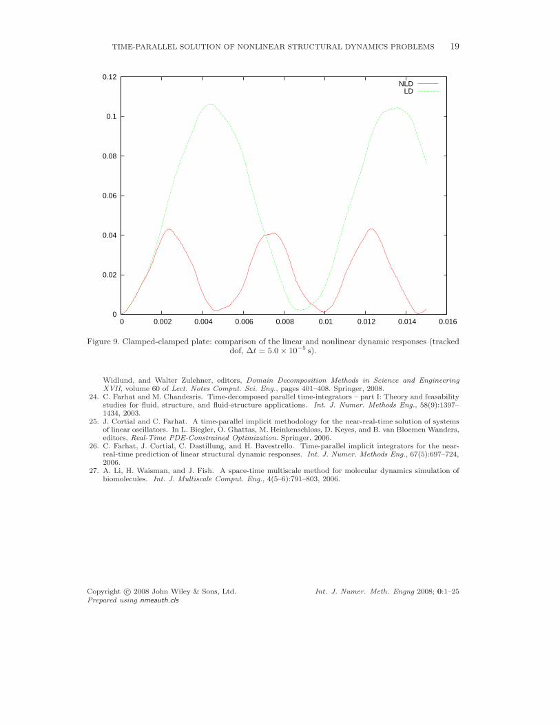
Fig. 8 shows a steel plate (E = 2 × 1011 N/m2, ν = 0.3) of length 1.0 m, width 0.2 m andthickness 0.02 m that is clamped at both ends. It is discretized by 160 × 4 × 2 = 1280 8-noded solid elements and 7155 unconstrained dof. At t0 = 0 s, a line force of magnitudeF = 8 × 104 N/m is applied at its middle, along its width. At this magnitude level, thedynamic response of the structure is in the nonlinear regime (see Fig. 9). All computationalresults associated with this problem are reported for the vertical displacement dof at the centerof the plate and for the time-interval [0 s, 1.5 × 10−2 s].

The computational time-step on the fine time-grid is set to ∆t = 5.0× 10−5 s. Fig. 10 whichcompares the structural responses predicted by the chosen ITA for this time-step, a ten-foldlarger one ∆t = 5.0× 10−4 s and a ten-fold smaller time-step ∆t = 5.0× 10−6 s shows that thevalue ∆t = 5.0 × 10−5 s is well-chosen.

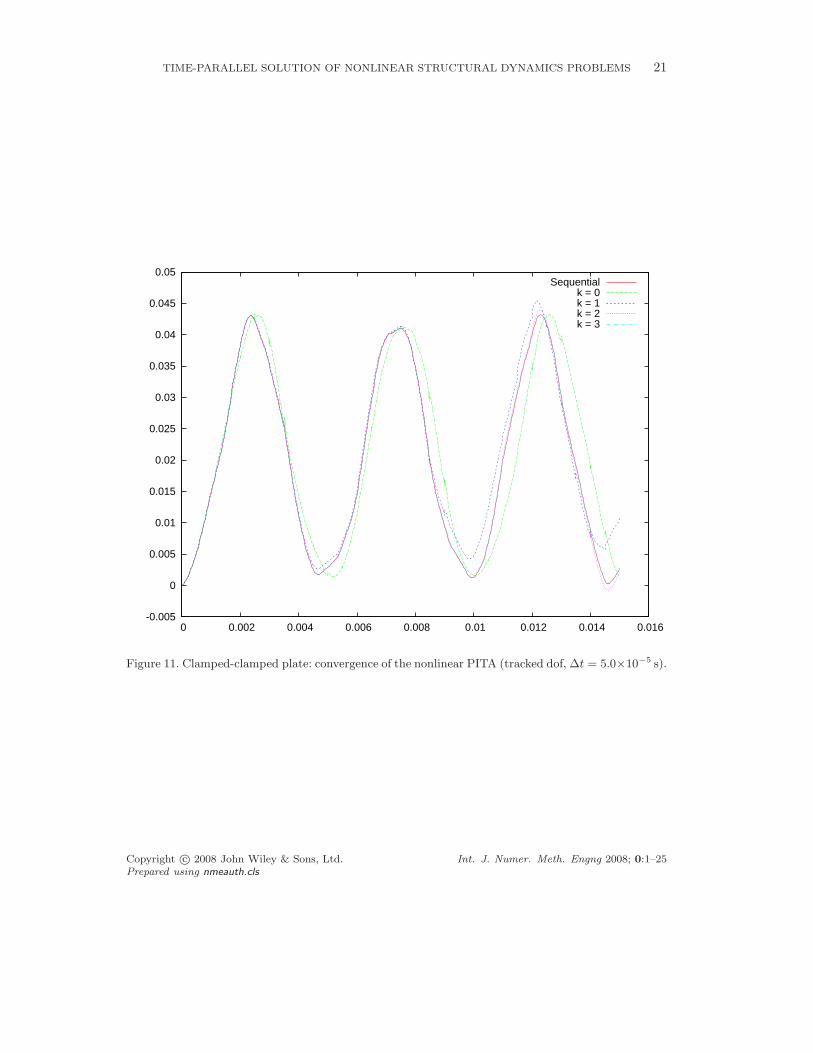
Next, the time-interval [0 s, 1.5 × 10−2 s] is partitioned into Nts = 30 slices so that∆T = 5 × 10−4s and J = 10. The nonlinear PITA is equipped with the local basis updatestrategy defined by (40) and (41) and the local metric (42), and is applied to the predictionof the vibrations of the plate. In this case, it converges in four iterations as shown in Fig. 11.

Next, the nonlinear PITA computation described above is repeated using the global basis



-7

-6

-5

-4

-3

-2

-1

0

1

2

0 5 10 15 20 25 30

Sequentialk = 0k = 1k = 2

Figure 5. Spherical cap: convergence of the nonlinear PITA (tracked dof, ∆t = 0.1 s).

update strategy (39). Fig. 12, which reports the magnitude of the jumps on the coarse time-grid of the solutions at the fourth iteration, reveals that when equipped with either consideredlocal basis update strategy, the nonlinear PITA behaves almost identically. This highlights theadvantage of the local basis update strategy given that it is computational more efficient thatits global counterpart.

The solution of this problem by the chosen ITA on a single processor of the considered Linuxcluster consumes T ITA = 172.5 s. Using 30 processors of the same cluster and the chosen ITAon the coarse-time grid to generate the initial seeds, the solution of the same problem bythe nonlinear PITA consumes T PITA

k=3 = 81 s when the local basis update strategy is selected,and 83 s when the global one is chosen. Each of these two CPU timings includes 33 s spenton generating the initial solution during Step 0. Hence, in either case, PITA accelerates thetime-to-solution by a factor greater than 2. To improve this speed-up factor, the nonlinearPITA computation is repeated and this time, the seeds Y i

0 , 0 ≤ i ≤ Nts −1 are first computedon a coarser mesh with 80×4×2 = 640 8-noded solid elements (3555 unconstrained dof) theninterpolated on the original mesh. Using this strategy for implementing Step 0 which was firstdiscussed in [26], the solution of the problem described above by the nonlinear PITA consumesT PITA

k=3 = 69 s on 30 processors, which corresponds to a speed-up factor greater than 2.5.



0

0.2

0.4

0.6

0.8

1

1.2

1.4

1.6

0 5 10 15 20 25 30

Sequentialk = 0k = 1k = 2

Figure 6. Convergence of the proposed nonlinear PITA framework: comparison of the approximationerror of the PITA (difference between the PITA and ITA solutions) and the time-discretization error

of the ITA (tracked dof, ∆t = 0.1 s).

6. SUMMARY AND CONCLUSIONS

In applications involving a relatively small number of degrees of freedom (i.e. robotics,multibody dynamics, protein folding, etc.), the spatial computations within each time-step offerlittle prospect for parallelism or for utilizing efficiently a large number of available processors.This lack of scalabilty becomes a significant drawback when the spatial domain is well resolvedbut massively parallel ressources are available for reducing the time-to-solution. It becomeseven more critical when real-time response is to be achieved. In both cases, time-parallelismbecomes desirable even if realized at the expense of parallel efficiency. However, time-steppingis sequential in nature. Therefore, parallelizing a computation across the time domain hasalways been a challenge. In a previous work, a unique Parallel Implicit Time-Integration(PITA) methodology was developed for the case of linear structural dynamics problems. Inthis paper, a nonlinear extension of this PITA framework is presented. Its application to thetime-parallelization of sample transient dynamic plate and shell problems reveals a potentialfor significantly reducing the time-to-solution associated with nonlinear structural dynamicsanalyses.



-8

-7

-6

-5

-4

-3

-2

-1

0

1

2

0 5 10 15 20 25 30

Sequentialkiter = 1kiter = 3

Figure 7. Spherical cap: numerical instabilities experienced by the nonlinear PITA when equippedwith Qi = I (tracked dof, ∆t = 0.1 s).

REFERENCES

1. J. White, A. Sangiovanni-Vincentelli, F. Odeh, and A. Ruehli. Waveform relaxation: Theory and practice.Trans. Soc. Comput. Simul., 2:95–133, 1985.

2. A. Lumsdaine and D. Wu. Krylov subspace acceleration of waveform relaxation. SIAM J. Numer. Anal.,41(1):90–111, 2003.

3. Stefan Vandewalle and Robert Piessens. On dynamic iteration methods for solving time-periodicdifferential equations. SIAM Journal on Numerical Analysis, 30(1):286–303, 1993.

4. K. Burrage. Parallel methods for initial value problems. Appl. Numer. Math., 11(1–3):5–25, 1993.5. S. Vandewalle and E. Van de Velde. Space-time concurrent multigrid waveform relaxation. Ann. Numer.

Math., 1:347–360, 1994.6. G. Horton, S. Vandewalle, and P. Worley. An algorithm with polylog parallel complexity for solving

parabolic partial differential equations. SIAM J. Sci. Comput., 16:531–541, 1995.7. G. Horton and S. Vandewalle. A space-time multigrid method for parabolic PDEs. SIAM J. Sci. Comput.,

16:848–864, 1995.8. S. Ta’asan and H. Zhang. Fourier-Laplace analysis of multigrid waveform relaxation method for hyperbolic

equations. BIT, 36(4):831–841, 1996.9. P. Amodio and L. Brugnano. Parallel implementation of block boundary value methods for ode’s. J.

Comput. Appl. Math., 78:197–211, 1997.10. L. Brugnano and D. Trigiante. Solving differential problems by multistep initial and boundary value

methods, volume 6 of Stability and Control: Theory, Methods and Applications. Gordon and BreachScience Publishers, Amsterdam, 1998.

11. J. Nievergelt. Parallel methods for integrating ordinary differential equations. Commun. ACM, 7(12):731–



Figure 8. Clamped-clamped plate: finite element mesh (the blue arrows indicate the constrained dofand the red arrows indicate the uniform line loading).

733, 1964.12. M. Kiehl. Parallel multiple shooting for the solution of initial value problems. Parallel Computing,

20(3):275–295, 1994.13. A. Bellen and M. Zennaro. Parallel algorithms for initial-value problems for difference and differential

equations. J. Comput. Appl. Math., 25:341–350, 1989.14. P. Chartier and B. Philippe. A parallel shooting technique for solving dissipative ODE’s. Computing,

51(3-4):209–236, 1993.15. J. Erhel, B. Philippe, and S. Rault. Parallelisation de calculs d’orbites. Rapport de recherche 3150,

INRIA, 1997.16. S. Rault. Algorithmes Paralleles pour le Calcul d’Orbites. PhD thesis, Universite Rennes I, 1998.17. P. Saha, J. Stadel, and S. Tremaine. A parallel integration method for solar system dynamics. Astron.

J., 114:409–415, 1997.18. J. L. Lions, Y. Maday, and G. Turinici. Resolution d’EDP par un schema en temps “parareel”. C. R.

Acad. Sci. Paris Ser. I Math., 332(7):661–668, 2001.19. Y. Maday and G. Turinici. A parareal in time procedure for the control of partial differential equations.

C. R. Acad. Sci. Paris Ser. I Math., 335(4):387–392, 2002.20. G. Bal and Y. Maday. A “parareal” time discretization for non-linear PDE’s with application to the pricing

of an American put. Recent developments in domain decomposition methods (Zurich, 2001), Lect. NotesComput. Sci. Eng., 23:189–202, 2002.

21. G. Bal. On the convergence and the stability of the parareal algorithm to solve partial differentialequations. In R. Kornhuber, R.H.W. Hoppe, D.E. Keyes, J. Periaux, O. Pironneau, and J. Xu, editors,Domain Decomposition Methods in Science and Engineering, volume 40 of Lect. Notes Comput. Sci. Eng.,pages 425–432. Springer, 2004.

22. M. Gander and S. Vandewalle. Analysis of the parareal time-parallel time-integration method. ReportTW 443, Katholieke Universiteit Leuven, 2005.

23. G. Bal and Q. Wu. Symplectic parareal. In Ulrich Langer, Marco Discacciati, David E. Keyes, Olof B.



0

0.02

0.04

0.06

0.08

0.1

0.12

0 0.002 0.004 0.006 0.008 0.01 0.012 0.014 0.016

NLDLD

Figure 9. Clamped-clamped plate: comparison of the linear and nonlinear dynamic responses (trackeddof, ∆t = 5.0 × 10−5 s).

Widlund, and Walter Zulehner, editors, Domain Decomposition Methods in Science and EngineeringXVII, volume 60 of Lect. Notes Comput. Sci. Eng., pages 401–408. Springer, 2008.

24. C. Farhat and M. Chandesris. Time-decomposed parallel time-integrators – part I: Theory and feasabilitystudies for fluid, structure, and fluid-structure applications. Int. J. Numer. Methods Eng., 58(9):1397–1434, 2003.

25. J. Cortial and C. Farhat. A time-parallel implicit methodology for the near-real-time solution of systemsof linear oscillators. In L. Biegler, O. Ghattas, M. Heinkenschloss, D. Keyes, and B. van Bloemen Wanders,editors, Real-Time PDE-Constrained Optimization. Springer, 2006.

26. C. Farhat, J. Cortial, C. Dastillung, and H. Bavestrello. Time-parallel implicit integrators for the near-real-time prediction of linear structural dynamic responses. Int. J. Numer. Methods Eng., 67(5):697–724,2006.

27. A. Li, H. Waisman, and J. Fish. A space-time multiscale method for molecular dynamics simulation ofbiomolecules. Int. J. Multiscale Comput. Eng., 4(5–6):791–803, 2006.



0

0.005

0.01

0.015

0.02

0.025

0.03

0.035

0.04

0.045

0 0.002 0.004 0.006 0.008 0.01 0.012 0.014 0.016

Delta t = 5.0e-5 sDelta t = 5.0e-4 sDelta t = 5.0e-6 s

Figure 10. Clamped-clamped plate: convergence time-step of the chosen nonlinear (sequential) ITA(tracked dof).



-0.005

0

0.005

0.01

0.015

0.02

0.025

0.03

0.035

0.04

0.045

0.05

0 0.002 0.004 0.006 0.008 0.01 0.012 0.014 0.016

Sequentialk = 0k = 1k = 2k = 3

Figure 11. Clamped-clamped plate: convergence of the nonlinear PITA (tracked dof, ∆t = 5.0×10−5 s).



0

1e-05

2e-05

3e-05

4e-05

5e-05

6e-05

7e-05

0 0.002 0.004 0.006 0.008 0.01 0.012 0.014 0.016

Local base updateGlobal base update

Local base update / Seed on coarser meshGlobal base update / Seed on coarser mesh

Figure 12. Clamped-clamped plate: magnitude of the jumps associated with the nonlinear PITA afterfour iterations using two different basis update strategies (tracked dof, ∆t = 5.0 × 10−5 s)

.


A Time-Parallel Implicit Method for Accelerating the...

Documents

Transcript of A Time-Parallel Implicit Method for Accelerating the...