A time machine for free fall into the past

Davide Fermi a, Livio Pizzocchero b

a,b Dipartimento di Matematica, Universita di MilanoVia C. Saldini 50, I-20133 Milano, Italy

and Istituto Nazionale di Fisica Nucleare, Sezione di Milano, Italy

a e–mail: davide.fermi@unimi.itb e–mail: livio.pizzocchero@unimi.it

Abstract

Inspired by some recent works of Tippett-Tsang and Mallary-Khanna-Price, we present a newspacetime model containing closed timelike curves (CTCs). This model is obtained postulating anad hoc Lorentzian metric on R4, which differs from the Minkowski metric only inside a spacetimeregion bounded by two concentric tori. The resulting spacetime is topologically trivial, free ofcurvature singularities and is both time and space orientable; besides, the inner region enclosedby the smaller torus is flat and displays geodesic CTCs. Our model shares some similaritieswith the time machine of Ori and Soen but it has the advantage of a higher symmetry in themetric, allowing for the explicit computation of a class of geodesics. The most remarkable featureemerging from this computation is the presence of future-oriented timelike geodesics starting froma point in the outer Minkowskian region, moving to the inner spacetime region with CTCs, andthen returning to the initial spatial position at an earlier time; this means that time travel to thepast can be performed by free fall across our time machine. The amount of time travelled into thepast is determined quantitatively; this amount can be made arbitrarily large keeping non-largethe proper duration of the travel. An important drawback of the model is the violation of theclassical energy conditions, a common feature of many time machines. Other problems emergefrom our computations of the required (negative) energy densities and of the tidal accelerations;these are small only if the time machine is gigantic.

Keywords: general relativity, closed timelike curves, time machines, energy conditions.

AMS Subject classifications: 83C05, 83C20 .

PACS: 04.20.Cv, 04.20.Gz, 04.90.+e .

arX

iv:1

803.

0821

4v3

[gr

-qc]

6 S

ep 2

018

1 Introduction

The construction of spacetime geometries admitting time travels is a recurrent subject in generalrelativity; within this framework, a time travel is usually described in terms of a closed timelikecurve (CTC).Excellent surveys on the subject were written by Thorne [39] and Lobo [23]. A threefold classificationof the existing literature has been proposed in a recent work of Tippett and Tsang [24]; we willintegrate the scheme of these authors with the addition of a fourth class, which leads to the followingdescription.

First class: exact solutions of the Einstein equations (typically with high symmetry, in many caseswith strong angular momentum). This streamline originated from Godel’s solution [14], describing astationary and homogeneous universe filled with rotating dust (and with a fine-tuned cosmologicalconstant); in this cosmological model, each event belongs to a CTC. Prior to Godel’s work, vanStockum [44] had solved the Einstein equations in presence of a rigidly rotating, infinite cylinderof dust (and with zero cosmological constant); the existence of CTCs in this spacetime was notedmuch later by Tipler [41]. To proceed, let us recall the Taub-NUT spacetime [29, 38], a spatiallyhomogeneous, vacuum solution with topology R × S3; the existence of CTCs in this model waspointed out by Misner [25], who also proposed a two-dimensional analogue of this geometry [26](see also the detailed analysis given by Thorne in [40]).The Kerr rotating black hole [19] also possesses CTCs which, however, are hidden behind an eventhorizon; indeed, these curves appear in the maximal extension of Kerr’s solution, near the ringsingularity (see, e.g., [17]). Tippett and Tsang also mention the Tomimatsu-Sato rotating, vacuumspacetime [43] (a generalization of Kerr’s model) and some spacetimes with moving cosmic strings.Especially, they refer to the papers of Gott [15] and of Deser, Jackiw, ’t Hooft [3]; in addition tothese references, we would also cite a paper of Grant [16] (considering a generalized version of Misnerspace, closely related to Gott’s model) and the very recent work of Mallary, Khanna and Price [24](who examine the existence of CTCs in a spacetime containing naked line singularities).

Second class: ad hoc built spacetimes, i.e., geometries specifically projected to produce CTCs.In these cases, the metric is given and the stress-energy tensor is derived a posteriori from theright-hand side of the Einstein equations; the undesired, exotic features emerging from this con-struction (typically, the violation of the standard energy conditions) are regarded as secondaryissues. Probably, the most influential papers in this class are those of Ori and Soen [32, 33, 34, 37].In particular, [34, 37] present a time machine with a toroidal spatial core, surrounded by a regionwhere the spacetime metric is conformally flat. CTCs are developed inside the toroidal region whenthe external time coordinate reaches a specific value, and violations of the energy conditions appearsimultaneously.The cited work of Tippett and Tsang [42] also belongs to this class. Therein, two flat spacetimegeometries are connected via a curved transition region, where the energy conditions are violated;the inner flat region contains CTCs. The model of [42] is simpler than the Ori-Soen spacetime inmany aspects, but a price must be paid for this: this spacetime is not time-orientable, and nakedcurvature singularities appear in the transition region.

Third class: ad hoc geometries originally designed to allow hyperfast space travel, which have naturalvariants possessing CTCs. Let us mention the celebrated Alcubierre’s warp drive [1], allowing forsuperluminal motion of a spaceship, and the improvements of this model suggested by Krasnikov,Everett and Roman [8, 20]; some of these authors also indicated how to use warp drives to produceCTCs [7, 20], developing a qualitative idea of Hawking [18]. As for the second class, these geometriesare generally postulated and the stress-energy tensor is subsequently obtained from the Einsteinequations; the standard energy conditions are violated, a fact that was proven to be unavoidable byOlum [30] if one adopts a specific definition of superluminal travel arrangement, proposed by thisauthor.

1

The third class also contains wormhole-type geometries (which, again, violate the energy conditions);notably, the static wormhole of Ellis, Morris and Thorne [5, 27] can be converted into a time machineby accelerating one of its two mouths, as shown by Morris, Thorne and Yurtsever [28]. (Let us alsomention a related paper by Echeverria, Klinkhammer and Thorne [4], mentioned later in connectionwith the paradoxes of time travels.)Fourth class. This is formed by just one model by Ori [35], which has connections with the first twoclasses but fits none of them exactly. A striking feature of this model is that it presents no violationof the energy conditions, since its matter content consists only of ordinary dust (or vacuum). Thespacetime of [35] is the union of three regions M0,M1 and M2. M0 is an internal, toroidal vacuumcore containing CTCs, with a “pseudo-Schwarzschild” metric obtained from the usual Schwarzschildline element performing a Wick rotation on the polar angle θ. M2 is an external, asymptoticallyflat vacuum region with the usual Schwarzschild metric outside a sphere. M1 is an intermediateregion, called the envelope, matching M0 and M2; this is filled with dust of non-negative density.We have pointed out that the spacetime metric is given a priori in M0 and M2, so there is a partialresemblance with the time machines of the second class; the situation is very different in the envelopeM1, where the metric is described as the solution of the Einstein equations with suitable Cauchydata. The above solution is not explicitly known, so the appearance of pathological structures(including black holes) cannot be excluded; a numerical investigation of these issues was indicatedin [35] as a goal for future works, and is still pending to the best of our knowledge.The possibility of time travels originates well known paradoxes, which were analysed by Friedmanet al. [12] and by Frolov and Novikov [13] (see Ch. 16 and the literature cited therein). Echeverria,Klinkhammer and Thorne [4] considered the Cauchy problem for a billiard ball in two exemplifyingspacetimes with CTCs generated by wormholes; due to the interaction of the ball with copies ofitself emerging from time travels, certain initial data for the Cauchy problem produce infinitelymany solutions (against the conventional expectation of one solution at most).Another paradoxical aspect of time machines is the appearing of divergences in the observables ofsemiclassical or quantized field theories. A result of this kind was obtained by Krasnikov [21] and canbe described as follows: under precise technical conditions, a spacetime describing the creation ofa time machine contains “almost closed” null geodesics, returning again and again to an arbitrarilysmall region where they are perceived as a “multi-photon bundle” of arbitrarily large energy. Theproblem of infinities was discussed by Hawking [18] for quantum field theories on spacetimes withCTCs; here the author considered a case study in which divergences exist even after renormalization,and he suggested that this should happen typically. To overcome the problem, Hawking formulatedthe famous chronology protection conjecture: the laws of (quantum) physics forbid CTCs. Theviewpoint of Hawking has been discussed elsewhere, and even questioned (see, in particular, acounterexample suggested by Li-Xin Li [22]).Dealing with the above mentioned paradoxes and problems is not among our purposes; here, wejust propose to enrich the second class of spacetimes with time travels, introducing a new model(which violates the energy conditions). In setting up this model, we were mainly stimulated by thepaper of Tippett-Tsang [42] (the work of Mallary, Khanna and Price [24] also gave us some generalmotivation to consider this subject); later on we realized that our construction has a closer contactwith the model of Ori-Soen [33, 34, 37].Our model is topologically trivial, possesses no curvature singularity, and is both space and timeorientable; it consists of a toroidal “time machine”, which contains CTCs and is surrounded byflat Minkowski space. These features resemble the Ori-Soen geometry, where a toroidal machine issurrounded by a conformally flat spacetime region; however, there are relevant differences betweenthat model and ours.Let us first point out the technical differences in the metric structure; later on, we will emphasizetheir physical implications. Differently from the Ori-Soen model (and similarly to the one of Tippett-

2

Tsang), our metric is non-flat only in a transition region individuated by two concentric tori Tλ,TΛ,with the same major radius R and minor radii λ,Λ; moreover, our metric exhibits more manifestsymmetries, which allow us to reduce to quadratures the Lagrange equations for a class of geodesicmotions (both outside and inside the time machine). Using these exact solutions, we can prove thefollowing: a freely falling observer (with suitable initial velocity) can start a trip at a spacetimepoint (t0 = 0,x0) in the outer Minkowskian region, fall into the time machine, re-emerge from it andfinally return to its initial space position x0 at a time t2 < 0 (where time and position are measuredwith respect to an inertial frame for the outer Minkowskian region; the subscript 2 to indicate theend of the travel is naturally suggested by our computations in Section 6). Obviously enough, onecan reinterpret this in terms of a CTC crossing the time machine (to close the observer’s worldline,it suffices to add a segment corresponding to the observers’ permanence at x0 from time t2 < 0 totime t0 = 0).Independently of the last remark, we think that time travel from (t0 = 0,x0) to (t2 < 0,x0) viafree fall across the time machine is the most interesting aspect of this model. We do not knowwhether such a time travel is possible in the Ori-Soen model, since these authors just pointed outthe existence of CTCs inside their time machine; let us also mention that the explicit computationof geodesic motions in the Ori-Soen metric is a non-trival affair, so it is difficult to ascertain thepossibility of a time travel similar to ours via free fall.Let us illustrate other features of the time travel from (t0 = 0,x0) to (t2 < 0,x0) in our model. Firstof all, adjusting suitably the initial velocity one can make |t2| arbitrarily large: in other terms, theobserver can go back into the past as far as he/she wants. Moreover, the duration τ2 of the timetravel according to the observer’s clock (i.e., the proper time along the observer’s world line) canbe made arbitrarily small: to this purpose, the observer must start his/her trip with a sufficientlylarge Lorentz factor with respect to the outer Minkowski frame. In this way the observer can goback into his/her past, say, of one billion years while his/her clock indicates a duration of only oneyear for the trip.To conclude the analysis of our model, we estimate the tidal acceleration experienced by a freelyfalling extended body when it crosses the transition region inside the time machine. We also deter-mine the energy densities measured by two kinds of observers: some suitably defined, “fundamental”observers and, alternatively, the freely falling observers performing a time travel (to this purpose,we adopt the previously mentioned idea to derive the stress-energy tensor from the metric via theEinstein equations). As expected, the tidal accelerations and the energy densities (of both kinds)vanish identically in the outer Minkowskian region and in the flat region inside the machine; in thetransition region between Tλ and TΛ, the tidal accelerations are non-zero and negative densitiesappear, yielding violations of the standard energy conditions.Both the tidal accelerations and the energy densities are inversely proportional to the square of themajor radius R (if the minor radii λ,Λ are comparable with it); so, these quantities are small ifthe time machine is gigantic. Indeed, our analysis is fully quantitative and exemplified by tableswith numerical values. If the radius R is astronomical (say, 100 light years), the tidal accelerationis sustainable for a human being, even for certain ultra-relativistic motions, and the energy densityaccording to a fundamental observer has an absolute value much smaller than 1gr/cm3 (in unitswhere c = 1); the energy density measured during free fall is below 1gr/cm3 even for some ultra-relativistic initial speeds (1).

Let us describe the organization of the present work. In Section 2 we introduce the spacetimeT describing our time machine; this is the base manifold R4, equipped with a suitably definedLorentzian metric g. The main characters of this section are a set of “cylindrical” spacetime coordi-

1These considerations about the energy density are not related to the evaluation of the effects produced on a freelyfalling observer by the exotic matter in the transition region between the tori Tλ,TΛ. As a matter of fact, free fall ispossible only if no direct interaction is assumed between the observer and this exotic matter.

3

nates (t, ϕ, ρ, z), the previously mentioned pair of concentric tori Tλ,TΛ and a sufficiently regularshape function X that equals 1 inside Tλ and vanishes identically outside TΛ; explicit choices forX are proposed in Appendix A.In Section 3 we exhibit an orthonormal tetrad (E(α))α∈0,1,2,3 for T, and use it to induce time andspace orientations. Contextually we introduce the “fundamental observers”, whose worldlines arethe integral curves of the timelike vector field E(0). In Section 4 we discuss some evident symmetriesof T and their physical implications.In Section 5 we consider the Lagrangian formalism for the causal geodesics in T; in particular, usingthe previously mentioned symmetries we reduce to quadratures the computation of causal geodesicsin the plane z = 0. Section 6 is the core of the present work: here, we use the previously establishedresults to prove the existence of a timelike geodesic (with fine-tuned initial velocity) which starts atany point in the outer Minkowskian region at time t0 = 0, crosses the tori TΛ,Tλ and eventuallyreturns to its initial spatial position at time t2 < 0. Certain integrals in the quadrature formulasfor the geodesics are analysed in Appendix B.In Section 7 and in the related Appendix C we discuss the tidal forces experienced by an extendedbody whose particles fall freely along geodesics as in Section 6. Section 8 and the related AppendixD deal with the energy densities measured by fundamental and freely falling observers, and pointout the violation of the classical energy conditions.

Some of the results presented in this paper have been derived using the software Mathematica forboth symbolic and numerical computations.

2 Description of the model

To begin with, let us consider the 4-dimensional Minkowski spacetime M = (R4, η), where η denotesthe usual, flat Lorentzian metric on the base manifold R4. We fix the units of measure so that thespeed of light is c = 1 (2); moreover, we introduce on R4 = R × R3 a set of coordinates (t, ϕ, ρ, z)where t is the natural coordinate on R and (ϕ, ρ, z) ∈ R/(2πZ)×(0,+∞)×R are standard cylindricalcoordinates on R3, so that the line element ds2

0 corresponding to the Minkowski metric η reads

ds20 = − dt2 + ρ2dϕ2 + dρ2 + dz2 . (2.1)

Next, let us fix λ,Λ, R ∈ (0,+∞) such that λ < Λ < R and consider in R3 the pair of concentrictori

T` :=√

(ρ−R)2 + z2 = ` (

` = λ,Λ)

(2.2)

(see Figure 1 for a graphical representation of these tori, having a common major radius R andminor radius λ or Λ).In addition, we introduce a regular function that equals 1 in the region inside Tλ and vanishesidentically in the region outside TΛ (3); more precisely, we set

X (ρ, z) := H(√

(ρ/R− 1)2 + (z/R)2), (2.3)

where H ∈ Ck([0,+∞);R) (k ∈ 2, 3, ...,∞) is an assigned shape function, such that

H(y) = 1 for y ∈ [0, λ/R] , H(y) = 0 for y ∈ [Λ/R,+∞) (2.4)

(see Figure 2; Appendix A suggests a possible choice H = H(k)).

2Let us stress that we do not set the universal gravitational constant to be G = 1.3Obviously enough, these two regions are defined, respectively, by the inequalities

√(ρ−R)2 + z2 < λ and√

(ρ−R)2 + z2 > Λ.

4

Figure 1

Λ Rλ R

0.5 1y

0.5

1

ℋ

Figure 2

Fig. 1: the concentric tori Tλ (in blue) and TΛ (in orange); here we have fixed λ/R = 3/5, Λ/R = 4/5.

Fig. 2: plot of a possible shape function H; here we have considered the function H = H(k) defined as in

Eq.s (A.3) (A.4) of Appendix A, with k = 3.

Inspired by the “interpolation strategies” of Alcubierre [1], Krasnikov [20], Tippett-Tsang [42] andother authors, we use the function X of Eq. (2.3) to introduce on R4 the quadratic form

ds2 :=

−[(

1−X (ρ, z))dt+ X (ρ, z) aRdϕ

]2+[(

1−X (ρ, z))ρ dϕ−X (ρ, z) b dt

]2+ dρ2 + dz2 .

(2.5)

Here, a, b ∈ R \ 0 are two parameters which are dimensionless in natural units with c = 1; thephysical meaning of these parameters will be clarified by the following analysis.Let us stress that, outside the larger torus TΛ, the quadratic form ds2 defined in Eq. (2.5) coincideswith the Minkowskian line element ds2

0 written in Eq. (2.1). On the other hand, inside the smallertorus Tλ, ds2 reduces to the flat line element

ds21 = − a2R2 dϕ2 + b2 dt2 + dρ2 + dz2 ; (2.6)

this shows that, contrary to what happens in the Minkowskian region outside TΛ, within Tλ thevariable ϕ ∈ R/(2πZ) plays the role of a time coordinate, while t ∈ R is a spatial coordinate.These considerations make evident that inside Tλ there are closed timelike curves (CTCs): theseare naturally parametrised by the periodic coordinate ϕ (see the beginning of Section 5 for furtherinformation on this topic).Anywhere on R4, Eq. (2.5) describes ds2 as an interpolation of ds2

0 and ds21 based on X . We write

g for the symmetric bilinear form associated to ds2, and (gµν) for its coefficients in a coordinatesystem (xµ). We claim that, when the parameters a, b ∈ R \ 0 fulfil the constraint

a b > 0 , (2.7)

the symmetric bilinear form g determined by ds2 is indeed a Lorentzian metric of class Ck (k > 2)on R4.To prove the above claim let us first point out that in the coordinate system (xµ) = (t, ϕ, ρ, z) wehave

det(gµν) = −[ρ(1−X (ρ, z)

)2+ a bR

(X (ρ, z)

)2]2. (2.8)

5

Notice that, under the assumption (2.7), the two addenda within the square brackets on the right-hand side of Eq. (2.8) are both non-negative and vanish simultaneously only for ρ = 0, thusdet(gµν) < 0 whenever ρ > 0. On the other hand, the axis ρ = 0 corresponds simply to asingularity of the cylindrical coordinate system (ϕ, ρ, z); this singularity disappears if one uses a setof standard Cartesian coordinates in a neighborhood of the said axis, where g coincides with theMinkowski metric η. The above considerations allow us to infer that g is everywhere non-degenerate.In addition, by direct inspection of the explicit expression (2.5) we can infer that 1 is an eigenvalueof (gµν) with multiplicity two (4); this constrains the remaining two eigenvalues to have oppositesigns in order to accomplish the previously established condition det(gµν) < 0. The latter remarksprove that (gµν) has three positive eigenvalues and a negative one, i.e., that g has signature (3, 1). Inorder to prove that the metric g is of class Ck it suffices to analyse the expressions of the coefficients(gµν) (depending on X ∈ Ck((0,+∞)× R)) in the coordinate system (t, ϕ, ρ, z), and to recall thatg coincides with η in a neighborhood of the axis ρ = 0.Of course, the Ck nature of g implies that the Riemann curvature tensor (along with all the asso-ciated curvature invariants) is of class Ck−2, hence free of singularities.Summing up, the modified line element (2.5) determines a new spacetime

T := (R4, g) , (2.9)

which is of course topologically trivial, contains CTCs and possesses no curvature singularity at all.In the forthcoming sections, we analyse in greater detail some interesting and non-trivial featuresof T. To perform this analysis, from now on we implement the condition (2.7) assuming that

a > 0 and b > 0 ; (2.10)

this causes no loss of generality since the complementary case where a < 0 and b < 0 can bestraightforwardly recovered via the change of coordinate t → −t (or, alternatively, ϕ → −ϕ).Furthermore, we restrict the attention to cases where the shape function

y 7→ H(y) is strictly decreasing for y ∈ (λ/R,Λ/R) , (2.11)

which grants in particular that

0 < X (ρ, z) < 1 for λ <√

(ρ−R)2 + z2 < Λ . (2.12)

The above requirements on H and X are not strictly necessary; however, they do in fact allow tolargely simplify some steps of the forthcoming analysis. Note that all the realizations H = H(k)

presented in Appendix A fulfil the condition (2.11).

2.1 A comparison with the Ori-Soen model

For their time machine, Ori and Soen postulate in [33] a line element ds2 on R4, using for the lattera coordinate system (t, ϕ, ρ, z) like ours; this line element depends on some parameters a, b, k > 0,q ∈ R and 0 < ˜< R and reads

ds2 =

F (t)[− dt2+ 2 X (ρ, z)

(a t dt− b

((ρ− R) dρ+ z dz

))ρ dϕ +

+(

1 + X (ρ, z)2(b2((ρ− R)2 + z2)− a2t2

))ρ2 dϕ2 + dρ2+ dz2

];

(2.13)

4To prove this statement, it suffices to notice that the components gµν with respect to the coordinates (t, ϕ, ρ, z)form a block matrix, whose only non-vanishing components are g00, g01 = g10, g11 and g22 = g33 = 1.

6

F (t) := 1 + q

(t− 1

a

)− k

(t− 1

a

)2

, X (ρ, z) := H(√(

ρ/˜− R/˜)2

+(z/˜

)2 ),

H(y) :=

(1− y4

)30 < y < 1 ,

0 y > 1 .

Like the function H, the metric is of class C2; thus, no curvature singularity occurs. The lineelement ds2 is conformally flat outside the toroidal region bounded by T˜ := (ρ− R)2+z2 = ˜2;inside T˜ the metric is not flat (not even conformally) and CTCs appear.Differently from ours, the line element ds2 depends on the coordinate t; CTCs and violations of theenergy conditions appear only for t > 1/a, i.e., there is an activation time for the machine. Theprice to pay for this t-dependence is that the Ori-Soen metric exhibits less symmetries than ours;due to this the explicit computation of its geodesics is problematic, as already mentioned in theIntroduction. In the forthcoming Sections 4-6 we will emphasize the symmetries of our metric anduse them to reduce to quadratures a class of geodesics, describing time travel by free fall. It is notclear whether these calculations would be possible in the Ori-Soen model; in any case, no attemptwas ever done in this direction.

3 A tetrad. Time and space orientations, fundamental observers

Let us proceed to determine for our model and orthonormal tetrad, consisting of four orthonormalvector fields (E(α))α∈0,1,2,3 of class Ck (k > 2). The facts stated hereafter can be readily inferredby direct inspection of the line element ds2 defined in Eq. (2.5); for this reason, we will not dwelltoo much on the related, elementary computations.Taking into account the explicit expression (2.5), it is natural to consider the set of 1-forms

e(0) :=(1−X (ρ, z)

)dt+ X (ρ, z) aRdϕ , e(1) :=

(1−X (ρ, z)

)ρ dϕ− X (ρ, z) b dt ,

e(2) := dρ , e(3) := dz ;(3.1)

these form a basis fulfillingg = ηαβ e

α ⊗ eβ , (3.2)

where (ηαβ) := diag(−1, 1, 1, 1) .Let us now consider the dual vector fields E(β), defined by 〈e(α), E(β)〉 = δαβ; due to Eq. (3.2), wehave

g(E(α), E(β)) = ηαβ . (3.3)

These vector fields are automatically granted to be of class Ck and have the explicit expressions (5)

E(0) =

(1−X (ρ, z)

)ρ ∂t + X (ρ, z) b ∂ϕ

ρ(1−X (ρ, z)

)2+ a bRX (ρ, z)2

, E(1) =

(1−X (ρ, z)

)∂ϕ − X (ρ, z) aR∂t

ρ(1−X (ρ, z)

)2+ a bRX (ρ, z)2

,

E(2) = ∂ρ , E(3) = ∂z .

(3.4)

Eq. (3.3) shows that E(0) and E(i) (i ∈ 1, 2, 3) are, respectively, timelike and spacelike everywhere.Therefore, we can use these vector fields to establish both time and space orientations for thespacetime T. In the following, we spend a few more words about the latter structures.

5Here we are implicitly making reference to Cartan’s formalism (see, e.g., Chapter 9 of [36]); in particular, due toEq. (3.2) (or (3.3)) we have the component identity

Eµ(α) = ηαβ gµν e(β)

ν (µ, ν, α, β ∈ 0, 1, 2, 3) ,

which can be used to infer the explicit expressions in Eq. (3.4).

7

Let us consider the expression for E(0) given in Eq. (3.4) and notice that, in the Minkowskianregion outside TΛ (where X = 0), this reduces to E(0) = ∂t; this indicates, amongst else, that E(0)

makes sense even at points where ρ = 0. On account of these facts, it is natural to define the futureas the time orientation containing E(0). Besides, from the said expression in Eq. (3.4) it followsthat E(0) = 1/(aR) ∂ϕ inside the region delimited by Tλ (where X = 1); considering the previouslyestablished convention on time orientation, this means that the coordinate vector field ∂ϕ is timelikeand future-oriented inside Tλ.As usual, in this paper the term observer is employed as a synonym of the expression “timelikeworldline” (with an obvious interpretation attached to it). In particular, any integral curve of thetetrad vector field E(0) will be called a fundamental observer. At any point of such a worldline

(with ρ > 0), E(1), E(2), E(3) span the orthogonal complement E⊥(0) which is the linear subspace ofinfinitesimal simultaneity corresponding to this observer. However, it can be easily checked thatE⊥(0) is not closed with respect to the commutators of vector fields which, by Frobenius theorem,

means that there does not exists a foliation of T into spacelike (hyper-)surfaces orthogonal to thefamily of fundamental observers mentioned above.Finally, let us discuss the possibility to define an orientation on the orthogonal complement E⊥(0),which could be understandably referred to as a “space orientation”. To this purpose let us firstremark that in the region outside TΛ we have E(1) = ρ−1∂ϕ, E(2) = ∂ρ and E(3) = ∂z, whichindicates, amongst else, that E(1) and E(2) are ill defined at ρ = 0. Keeping in mind this fact,

at all spacetime points with ρ > 0 we equip E⊥(0) with the orientation induced by the ordered

triplet (E(2), E(1), E(3)). To go on we note that, in the region outside TΛ (where E(0) = ∂t), E⊥(0) is

spanned as well by the vectors E(i) = ∂xi (i = 1, 2, 3), defined starting from the coordinate systemx1 = ρ cosϕ, x2 = ρ sinϕ, x3 = z. It can be easily checked that the triplets (E(2), E(1), E(3)) and

(E(1), E(2), E(3)) are equi-oriented at all spacetime points outside TΛ with ρ > 0 (6); moreover, since

the vectors E(i) also make sense at ρ = 0, we can use the triple (E(1), E(2), E(3)) to define a coherent

orientation of E⊥(0) at these points.

4 Symmetries of the model

First of all, let us remark that none of the tetrad vector fields E(α) (α ∈ 0, 1, 2, 3) considered inthe previous section is a generator of isometries for T, since none of them fulfils the Killing equationLE(α)

g = 0 (L denotes the Lie derivative). Nevertheless, the spacetime T does in fact possessesa number of self-evident symmetries, both discrete and continuous, which we are going to discussseparately in the following paragraphs.

Discrete symmetries. On the one hand, it can be easily checked by direct inspection that thetransformation with coordinate representation

(t, ϕ, ρ, z)→ (− t,−ϕ, ρ, z) (4.1)

preserves the line element ds2 of Eq. (2.5), thus describing a (discrete) symmetry of T. Let usnotice that under this transformation the vector fields E(0) and E(1) are mapped, respectively, to−E(0) and −E(1); on the contrary, E(2) and E(3) are left unchanged. Recalling that the tetrad(E(α))α∈0,1,2,3 determines the time and space orientations of T, we can say that the spacetime Tis in fact invariant under the simultaneous reversal of the time and space orientations.

6The peculiar ordering (E(2), E(1), E(3)) is used just to ensure this result of equi-orientation.

8

On the other hand, due to the specific choice (2.3) of the shape function X , it appears that ds2 isalso invariant under the transformation

(t, ϕ, ρ, z)→ (t, ϕ, ρ,− z) , (4.2)

i.e., under reflection across the plane z = 0. By direct inspection of the explicit expressions in Eq.(3.4) it can be readily inferred that, under the transformation (4.2), the vector fields E(0), E(1), E(2)

are left unchanged while E(3) is mapped to −E(3). Thus, T is invariant under reversal of the spaceorientation.Summing up, the previous arguments show that T is invariant both under the sole reversal of spaceorientation and under the simultaneous reversal of space and time orientations. Therefore, T is alsoinvariant under the sole reversal of the time orientation.

Killing vector fields and stationary limit surfaces. Let us now pass to the analysis of thecontinuous symmetries of T.First of all let us repeat that, outside the larger torus TΛ, the metric g of the spacetime underanalysis coincides with that of flat Minkowski spacetime; therefore, it can be readily inferred thatthis region admits a maximal, 10-dimensional algebra of Killing vector fields. The same conclusioncan be drawn for the region inside the smaller torus Tλ, since therein the metric g is flat as well.Next, let us pass to the analysis of global continuous symmetries. Since the metric coefficients donot depend on the coordinates t and ϕ, it can be inferred straightforwardly that both

K(0) := ∂t and K(1) := ∂ϕ (4.3)

are Killing vector fields.It can be checked by elementary computations that K(0) is timelike on Θ−(0), null on Σ(0) and

spacelike on Θ+(0), where

Θ±(0) :=X (ρ, z) ≷ (1 + b)−1

, Σ(0) :=

X (ρ, z) = (1 + b)−1

. (4.4)

Θ−(0) is the spacetime region in which the orbits of K(0), being timelike, can be interpreted as

observers; this contains the region outside TΛ (where X (ρ, z) = 0). Σ(0) is the boundary of the

region Θ−(0) and so, in the language of [2, 17], it is a stationary limit surface for K(0).

A similar analysis can be performed for the other Killing vector field K(1); this is timelike on Θ−(1),

null on Σ(1) and spacelike on Θ+(1), where

Θ±(1) :=X (ρ, z) ≶ (1 + aR/ρ)−1

, Σ(0) :=

X (ρ, z) = (1 + aR/ρ)−1

. (4.5)

Θ−(1) contains the region inside Tλ (where X (ρ, z) = 1); its boundary Σ(1) is a stationary limitsurface for K(1).With our assumptions on the shape function H, it can be easily checked that both Σ(0) and Σ(1)

are timelike hypersurfaces (7); so, in particular, neither of them is a Killing horizon for K(0) or

7As an example, let us account for this statement in the case of Σ(0). To this purpose, it should be recalled thatin the present work H(y) is assumed to be strictly decreasing for y ∈ (λ/R,Λ/R) (see the comments at the end ofSection 2). In consequence of this assumption, the surface Σ(0) can be described as

Σ(0) =F (ρ, z) := (ρ−R)2 + z2 −

[Λ− (Λ− λ)H−1(1/(1 + b)

)]2= 0

,

where H−1 denotes the local inverse of H in the interval (λ/R,Λ/R) (notice that 0 < 1/(1+b) < 1, since b > 0). Then,considering the vector field nF ≡ (nµF ) = (gµν(dF )ν) normal to Σ(0), it can be inferred by elementary computationsthat

g(nF , nF ) = 4[Λ− (Λ− λ)H−1(1/(1 + b)

)]2> 0 .

The above relation proves that nF is spacelike, which by definition is equivalent to say that Σ(0) is timelike (see, e.g.,Section 2.7 of [17]).

9

K(1). Besides, it appears that the positions and the shapes of Σ(0) and Σ(1) depend strongly on theparticular choices of the radii λ,Λ, R and of the parameters a, b > 0. In particular, recalling that weare assuming the shape function H(y) to be strictly decreasing for y ∈ (λ/R,Λ/R), it can be checkedby direct inspection of Eq.s (4.4) (4.5) that for a/b < 1− Λ/R (compare with the forthcoming Eq.(6.8)) there is a region of spacetime where a test particle cannot remain at rest neither with respectto observers in the outer Minkowskian region nor with respect to observers in the innermost regiondelimited by Tλ.

5 Results on causal geodesics

Here and in the rest of the paper, a geodesic in T will always be represented in terms of an affineparametrization ξ : τ 7→ ξ(τ); we will write ˙ for the derivative with respect to τ .Let us first remark that, in the region outside TΛ, all geodesics do in fact coincide with those of flatMinkowski spacetime; in particular, the orbits of the Killing vector field K(0) are timelike geodesicsin this region. Similar considerations hold for the flat spacetime region inside the smaller torus Tλ.Notably, as anticipated in Section 2, we have CTCs ξ : τ 7→ ξ(τ) with the following representationin coordinates (xµ) := (t, ϕ, ρ, z) :

(ξµ(τ)) =(t0, ϕ0 + Ω τ (mod 2π), ρ0, z0

), 0 6 τ 6 2π/Ω , (5.1)

where Ω > 0, t0 ∈ R, ϕ0 ∈ R/(2πZ) and ρ0 > 0, z0 ∈ R are such that 0 6√

(ρ0/R−1)2+(z0/R)2

< λ/R ; such a curve is future-oriented (8). In passing, let us also remark that the above curvescoincide with the orbits of the Killing vector field K(1) inside Tλ.

Let us now pass to the study of different causal geodesics, not necessarily confined outside TΛ orinside Tλ. As a matter of fact we are going to show in the subsequent Section 6 that, at least forsuitable choices of the parameters a, b and of the shape function H, there exist timelike geodesicswhich start from the region outside TΛ, cross both TΛ and Tλ and return outside TΛ; this fact isnot self-evident a priori and has non-trivial consequences to be discussed later on.To this purpose, let us first recall that any (affinely parametrised) geodesic can be characterized asa solution ξ of the Euler-Lagrange equations associated to the Lagrangian function (9)

L : TT→ R , L(X) :=1

2g(X,X

)(5.2)

whose representation in our usual coordinates is

L(xµ, xµ) =

−1

2

[ (1−X (ρ, z)

)t+ X (ρ, z) aR ϕ

]2+

1

2

[ (1−X (ρ, z)

)ρ ϕ−X (ρ, z) b t

]2+

1

2ρ2 +

1

2z2 .

(5.3)

For simplicity, from now on we restrict the attention to the plane z = 0 of T, that we equip withthe coordinates (xA)A∈0,1,2 := (t, ϕ, ρ). Our considerations involve the dimensionless variable

r := ρ/R ∈ (0,+∞) (5.4)

8The metric g of T has constant coefficients in coordinates (t, ϕ, ρ, z) in the region inside Tλ (where X = 1 andds2 has the form (2.6)); ξ is represented in these coordinates by an affine function of τ , so it is a geodesic. For0 6 τ 6 2π/Ω we have ξ(τ) = Ω ∂ϕ; this is a timelike vector, we now discuss its orientation. It is easily checkedthat g

(E(0)

(ξ(τ)

), ξ(τ)

)= − aRΩ < 0 (recall our assumption (2.10) and Eq. (3.4)); since we have chosen E(0) to be

everywhere future-oriented (see Section 3), the latter identity shows that ξ(τ) is future-oriented as well.9Of course, if X is tangent to T at a point p, g(X,X) stands for gp(X,X); the notation L(X) understands the

dependence on p. Similar remarks will never be repeated in the remainder of this paper.

10

and the function (see Eq.s (2.3) (2.4))

ρ ∈ (0,+∞) 7→ X (ρ, 0) = H(ρ/R) , H(r) := H(|r − 1|

), (5.5)

which fulfils, in particular,

H(r) = 0 for r ∈ (0, 1− Λ/R] ∪ [1 + Λ/R,+∞) ,

H(r) = 1 for r ∈ [1− λ/R, 1 + λ/R] .(5.6)

Let us write L for the Lagrangian L restricted to the (tangent bundle of the hyper-) plane z = 0.The coordinate representation of L is obtained setting z = 0, z = 0 in Eq. (5.3), and can be writtenas follows:

L(xA, xA

):=

−1

2

[ (1−H(ρ/R)

)t+ aR H(ρ/R) ϕ

]2+

1

2

[ρ(1−H(ρ/R)

)ϕ− bH(ρ/R) t

]2+

1

2ρ2.

(5.7)

It is readily checked that there are geodesics ξ of T lying in the plane z = 0, and that suchgeodesics coincide with the solutions of the Euler-Lagrange equations induced by L (10) (11).The Lagrange equations induced by L possess a maximal number of first integrals, and can be solvedby quadratures. The said first integrals are the energy and two conserved momenta; let us give moredetails on this subject.The energy function, defined via the general theory of Lagrangian systems, coincides with L due tothe purely “kinetic” nature of this Lagrangian. Thus L(ξ(τ)) = 1

2 g(ξ(τ), ξ(τ)) = const. along anysolution ξ of the Lagrange equations; this corresponds to the well known conservation law for thenorm of the velocity of any geodesic.We are mainly interested in causal geodesics, i.e., in null or timelike geodesics. In the null case, weobviously have

L(ξ) = 0 . (5.8)

In the timelike case, after possibly rescaling τ by a constant factor, we can arrange things so thatg(ξ, ξ) = −1 i.e.

L(ξ) = − 1

2, (5.9)

which is equivalent to saying that the parameter τ is proper time.To go on, let us notice that the explicit expression (5.7) for L does not depend explicitly on t, ϕ; so,the system admits as conserved quantities the canonical momenta (12)

pt :=∂L

∂t, pϕ :=

∂L

∂ϕ. (5.10)

10We have just stated that the geodesics in T are characterized by the Euler-Lagrange equations for L. One checksby elementary means that the equation (d/dτ)(∂L/∂z) − ∂L/∂z = 0 is fulfilled setting z(τ) := 0; this statementdepends crucially on the fact that (∂zX )(ρ, 0) = 0 (see Eq. (2.3)). The remaining Euler-Lagrange equations inducedby L coincide, if z(τ) = 0, with those associated to L.

11Notice that L could be seen as the Lagrangian associated to a 3-dimensional spacetime, obtained from T bysuppression of the coordinate z; because of this, all the considerations that follow could be interpreted in terms ofgeneric geodesics in this 3-dimensional space-time.

12In passing, let us remark that pt and pϕ are strictly related to the Killing vector fields K(0) and K(1), defined inEq. (4.3). More precisely, for each vector X tangent to z = 0 one has

pt(X) = g(K(0), X) , pϕ(X) = g(K(1), X) .

This is readily checked expressing pt(X), pϕ(X) in terms of the components t, ϕ, ρ of X, and comparing with thecoordinate expressions of g(K(0), X), g(K(1), X).

11

In hindsight, it is convenient to replace the momenta pt, pϕ with the related quantities

γ ≡ γ(ρ, t, ϕ) := − pt =[ (1−H(ρ/R)

)2 − b2 H(ρ/R)2]t +

(a+ b ρ/R

)H(ρ/R)

(1−H(ρ/R)

)R ϕ ,

(5.11)

ω ≡ ω(ρ, t, ϕ) := − pϕγ R

=

1

γ

(a+ b ρ/R

)H(ρ/R)

(1−H(ρ/R)

)t − 1

γ

[(ρ/R)2

(1−H(ρ/R)

)2− a2 H(ρ/R)2]R ϕ .

(5.12)

Note that both γ and ω are dimensionless; hereafter we show that γ > 0 in the situation in whichwe are mainly interested. To be precise, let us consider the case of a future-oriented causal curvepassing through the Minkowskian region outside TΛ (where ρ > R+ Λ and H = 0); then Eq. (5.11)gives

γ(ρ, t, ϕ) = t (5.13)

along the curve, implying that γ > 0. In particular, let us consider the case of a future-orientedtimelike curve parametrized by proper time τ ; in this case we have γ = t ≡ dt/dτ along the curve,indicating that γ is the familiar “Lorentz factor” of relativity in Minkowski spacetime. Thus γ > 1and the limits γ → 1+, γ → +∞ correspond, respectively, to non-relativistic and ultra-relativisticmotions with respect to the coordinate frame (t, ϕ, ρ, z).Eq.s (5.11) (5.12) are easily solved for t, ϕ in terms of ρ, γ, ω; this gives (13)

t(ρ, γ, ω) =

γ

[(ρ/R)2

(1−H(ρ/R)

)2− a2 H(ρ/R)2]

+(a+b ρ/R

)H(ρ/R)

(1−H(ρ/R)

)ω[

(ρ/R)(1−H(ρ/R)

)2+ a bH(ρ/R)2

]2 ,(5.14)

ϕ(ρ, γ, ω) =

γ

(a+b ρ/R

)H(ρ/R)

(1−H(ρ/R)

)−[(

1−H(ρ/R))2 − b2 H(ρ/R)2

]ω

R[(ρ/R)

(1−H(ρ/R)

)2+ a bH(ρ/R)2

]2 .(5.15)

In particular, the above relations give

t(ρ, γ, ω) = γ , ϕ(ρ, γ, ω) = − γ ω Rρ2

for ρ ∈ (0, R− Λ] ∪ [R+ Λ,+∞) , (5.16)

t(ρ, γ, ω) = − γ 1

b2, ϕ(ρ, γ, ω) = γ

ω

a2Rfor ρ ∈ [R− λ,R+ λ] . (5.17)

Notably, the first identity in Eq. (5.17) shows that t is (constant and) negative inside the smallertorus Tλ; in consequence of this, the coordinate time t decreases along future-oriented causalgeodesics in the region inside Tλ. This fact is crucial for the possibility of time travels to thepast, a topic to be discussed in more detail in the following Section 6.Now, let us consider the reduced Lagrangian

Lγ,ω(ρ, ρ) :=[L(xα, xα)−

((−γ) t+ (− γ ω R) ϕ

)]t= t(ρ,γ,ω), ϕ= ϕ(ρ,γ,ω)

(5.18)

(recall that − γ = pt and − γ ω R = pϕ); by direct computation, this can be expressed as

Lγ,ω(ρ, ρ) =1

2ρ2 − Vγ,ω(ρ) , (5.19)

13Notice that the denominators in Eq.s (5.14) (5.15) coincide, apart from overall multiplicative constant factors (−1and −R, respectively), with the metric determinant det(gµν) (see Eq. (2.8)) at (xµ) = (t, ϕ, ρ, 0); besides, recall thatdet(gµν) < 0 (see the considerations reported below Eq. (2.8)). These facts suffice to infer that the expressions in thecited equations are well defined whenever ρ > 0.

12

1- /R

1- /R 1+ /R

1+ /R

1 2r

-1.5

-1

-0.5

0

0.5

1

1.5

Vγ,ω

Figure 3a: ω = − 0.08.

1- /R

1- /R 1+ /R

1+ /R

1 2r

-4

-2

0

2

4

Vγ,ω

Figure 3b: ω = 0.08.

Fig.s 3a-3b: the potential Vγ,ω (black line) as a function of the dimensionless variable r := ρ/R, for λ/R = 3/5,

Λ/R = 4/5, a = 9/100, b = 10, γ = 1.1 and for two opposite choices of ω. In both cases, the shape function

H = H(k) is the one given in Eq.s (A.3) (A.4) of Appendix A, with k = 3. The red lines correspond to the

energy value E = −1/2.

where we have introduced the effective potential

Vγ,ω(ρ) :=(γ2

2

) [aH(ρ/R)−

(1−H(ρ/R)

)ω]2 − [(ρ/R)

(1−H(ρ/R)

)+ bH(ρ/R)ω

]2[(ρ/R)

(1−H(ρ/R)

)2+ a b H(ρ/R)2

]2 .(5.20)

Let us remark that Vγ,ω depends on the radial coordinate ρ only through the dimensionless ratior := ρ/R (we have taken this fact into account in Fig.s 3a-3b, showing the graphs of Vγ,ω as afunction of r for some choices of the parameters). Moreover,

Vγ,ω(ρ) =γ2

2

(R2 ω2

ρ2− 1

)for ρ ∈ (0, R− Λ] ∪ [R+ Λ,+∞) , (5.21)

Vγ,ω(ρ) = const. =γ2

2 a2

(a2

b2− ω2

)for ρ ∈ [R− λ,R+ λ] . (5.22)

Clearly, Lγ,ω can be interpreted as the Lagrangian function associated to a classical point particlemoving along the half-line (0,+∞), in presence of the potential Vγ,ω . The total energy of thisone-dimensional system, a conserved quantity, is

E :=1

2ρ2 + Vγ,ω(ρ) ; (5.23)

this is found to coincide with the Lagrangian L and this result, along with Eq.s (5.8) (5.9), gives

E =

0 for null geodesics ,

−1/2 for timelike geodesics .(5.24)

Of course, for each solution of the Euler-Lagrange equations, ρ(τ) (τ ∈ R) is confined within aconnected component of the region ρ ∈ (0,+∞) | Vγ,ω(ρ) 6 E and conservation of the totalenergy can be used to reduce to quadratures the computation of ρ(τ).Let us consider an interval [τi, τf ] ⊂ R and assume

sign ρ(τ) = σ ∈ ±1 for τi < τ < τf , ρ(τi) = ρi, ρ(τf ) = ρf . (5.25)

13

Then, on the said interval we have

ρ ≡ ρ(ρ,E, γ, ω) = σ√

2(E− Vγ,ω(ρ)

), (5.26)

whence

τf − τi = σ

∫ ρf

ρi

dρ√2(E− Vγ,ω(ρ)

) . (5.27)

In the case of a timelike geodesic (E = −1/2), the above equation gives the variation of the propertime along this part of the geodesic.Keeping the assumptions (5.25), let

t(τh) = th , ϕ(τh) = ϕh (h ∈ i, f)

and consider the maps [ρi, ρf ] 3 ρ 7→ t(ρ), ϕ(ρ) obtained composing the functions [τi, τf ] 3 τ 7→t(τ), ϕ(τ) with the inverse function ρ 7→ τ(ρ) of the map [τi, τf ] 3 τ 7→ ρ(τ). Then, using thenotation ′ ≡ d/dρ, we have

t′(ρ) =t(ρ, γ, ω)

ρ(ρ,E, γ, ω), ϕ′(ρ) =

ϕ(ρ, γ, ω)

ρ(ρ,E, γ, ω),

where t, ϕ, ρ are as in Eq.s (5.14), (5.15), (5.26). Using the explicit expression for ρ and integrating,we get

tf − ti = σ

∫ ρf

ρi

dρt(ρ, γ, ω)√

2(E− Vγ,ω(ρ)

) , (5.28)

ϕf − ϕi = σ

∫ ρf

ρi

dρϕ(ρ, γ, ω)√

2(E− Vγ,ω(ρ)

) (5.29)

(the last equality being understood mod 2π).In the subsequent sections we will confine the attention to the case of timelike geodesics (E = −1/2)and use the present results to show that an observer freely falling in the plane z = 0 can travelbackwards in time. No further discussion will be performed on null geodesics (E = 0); we plan toreturn to this subject in future works, where the present analysis of null geodesics will be used todiscuss the light signals emitted by the time traveller towards the outer Minkowskian region.

6 Free fall and time travel into the past

6.1 Free fall under special assumptions

Let us consider a massive test particle freely falling in the plane z = 0. The worldline of such aparticle is a timelike geodesic and can be analysed following the framework described in the previoussection with E = −1/2, i.e., using a proper time parametrization τ 7→ ξ(τ).We make the following assumptions (i)(ii), involving the initial conditions ξ(0), ξ(0) and the dimen-sionless parameters γ, ω associated to ξ (see Eq.s (5.11) (5.12)):

(i) We have

t(0) = 0 , t(0) > 0 , ϕ(0) = 0 , ρ(0) = ρ0 > R+ Λ , ρ(0) < 0 . (6.1)

The choices of t(0) and ϕ(0) are conventional, and imply no loss of generality. The conditiont(0) > 0 indicates that ξ(0) is future-oriented: by continuity, ξ(τ) will be future-oriented forall τ . The conditions on ρ(0) and ρ(0) mean that the particle is initially in the Minkowskianregion outside the larger torus TΛ, with radial velocity pointing towards TΛ.

14

(ii) The effective potential Vγ,ω defined in Eq. (5.20) fulfils

Vγ,ω(ρ)

> −1/2 for ρ ∈ (0, ρ1) ,= −1/2 for ρ = ρ1 ,< −1/2 for ρ ∈ (ρ1,+∞)

for some ρ1 ∈ (0, R− Λ) (6.2)

(this holds, e.g., in the case of Fig. 3b). Together with (i), this ensures that, for τ > 0, theradial coordinate ρ = ρ(τ) of the particle will decrease until a minimum value ρ1 and then itwill increase (we shall return on this later).

6.2 Implications of (i)(ii) on the parameters a, b, γ,ω

Firstly let us recall that, for a motion like the one under analysis, γ is the familiar Lorentz factorof special relativity (a fact already mentioned after Eq. (5.13)). In particular, we have the lowerbound γ > 1; moreover, the equality γ = 1 cannot be realized in the particular case that we areconsidering for this would imply that the three-velocity of the particle vanishes at τ = 0, againstthe assumption ρ < 0 of Eq. (6.1). In conclusion, we have

γ > 1 . (6.3)

Secondly we remark that, according to (ii), for suitable τ > 0 we have ρ(τ) ∈ [R − λ,R +λ]; for the same values of τ , Eq. (3.4) (with X (ρ, z) = 1) and Eq. (5.17) give E(0)(ξ(τ)) =

1/(aR) ∂ϕ and ϕ(τ) = γ ω/(a2R), which implies g(E(0)(ξ(τ)), ξ(τ)

)= − γ ω/a . On the other hand,

E(0)(ξ(τ)) and ξ(τ) have the same time orientation (indeed, they are both future-oriented); thus,

g(E(0)(ξ(τ)), ξ(τ)

)< 0. Recalling that we are assuming a > 0 (see Eq. (2.10)), the facts pointed

out above giveω > 0 . (6.4)

Let us recall that, according to Eq. (5.16), we have ϕ(0) = − γ ωR/ρ20; so, Eq. (6.4) implies ϕ(0) < 0.

To go on, let us consider the point ρ1 mentioned in Eq. (6.2). This can be readily determinedsolving the equation Vγ,ω(ρ1) = −1/2 with the expression (5.21) for Vγ,ω, which gives

ρ1 =R ω√

1− 1/γ2. (6.5)

The right-hand side of the above equation must belong to the interval (0, R − Λ), so we are forcedto assume that

ω√1− 1/γ2

< 1− Λ

R. (6.6)

Finally the condition Vγ,ω(ρ) < −1/2 in Eq. (6.2), required to hold for all ρ ∈ (ρ1,+∞), must befulfilled in particular for ρ ∈ [R − λ,R + λ] where Vγ,ω(ρ) has the constant value indicated in Eq.(5.22); this yields the inequality

γ2

2 a2

(a2

b2− ω2

)< − 1

2. (6.7)

By elementary manipulations, one finds that the constraints (6.3), (6.4), (6.6) and (6.7) imply

a

b< 1− Λ

R, γ >

√(1− Λ/R)2 + a2

(1− Λ/R)2 − a2/b2,

a

b

√1 +

b2

γ2< ω <

(1− Λ

R

)√1− 1

γ2

(6.8)

(note that the inequalities in the first line are equivalent to the relation ab

√1+ b2

γ2 <(1− Λ

R

)√1− 1

γ2 ).

The above arguments show that the assumptions (i)(ii) imply (6.8). Investigating the validity ofthe converse implication (6.8)⇒ (i)(ii) is a non trivial task, since the shape function H is implicitlyinvolved in the condition (ii); in any case, this problem is not relevant for our purposes.

15

6.3 The claimed time travel: qualitative features

The essential qualitative features of a timelike geodesic motion ξ under the assumptions (i)(ii) ofsubsection 6.1 have been sketched in the accompanying comments. To be more precise, the citedassumptions ensure that:

(a) for τ > 0, the coordinate ρ(τ) of the particle will decrease until reaching the minimum valueρ1 at a certain proper time τ1;

(b) after this, the coordinate ρ(τ) will increase and return to its initial value ρ0 at a proper timeτ2:

ρ(τ2) = ρ0 . (6.9)

To proceed, let us putt2 := t(τ2) , ϕ2 := ϕ(τ2) ; (6.10)

we claim that we can choose a, b, ρ0, γ, ω (and H) so that

t2 < 0 , (6.11)

ϕ2 = 0 (mod 2π) . (6.12)

Eq.s (6.9) (6.12) indicate that the final space position of the particle, as measured in the coordinateframe (t, ϕ, ρ, z), coincides with the initial position. Taking this into account, the inequality (6.11)means that the event ξ(τ2) (the end of the travel) is in the past of the initial event ξ(0) with respectto the chronological structure of the Minkowskian region outside TΛ. Note that t2 is the timeindicated at the end of the travel by a clock initially set to zero and kept at ϕ = 0, ρ = ρ0, z = 0during the whole travel of the freely falling particle. On the other hand, τ2 is the final time indicatedby a clock initially set to zero, which has travelled with the particle.All the above claims will be proved by the forthcoming quantitative analysis of the geodesic ξ. Wealso make a stronger claim: choosing appropriately a, b, γ, ω,H we can make |t2| arbitrarily large,i.e., go arbitrarily far in the past keeping τ2 (the proper duration of the trip) small with respect to|t2|.

6.4 The claimed time travel: quantitative analysis

For the moment, we consider any choice of a, b, ρ0, γ, ω (and H) fulfilling (i)(ii). Let us combine thegeneral rules (5.27) (5.28) and (5.29) for the variations of τ , t and ϕ with the qualitative features(a)(b) of the geodesic ξ under analysis; these imply, in particular, that σ = −1 on (0, τ1) and σ = 1on (τ1, τ2). Therefore, via the elementary identity −

∫ ρ1

ρ0+∫ ρ0

ρ1= 2

∫ ρ0

ρ1, we get

t2 = 2

∫ ρ0

ρ1

dρ t(ρ, γ, ω)√−1− 2Vγ,ω(ρ)

, ϕ2 = 2

∫ ρ0

ρ1

dρ ϕ(ρ, γ, ω)√−1− 2Vγ,ω(ρ)

,

τ2 = 2

∫ ρ0

ρ1

dρ√−1− 2Vγ,ω(ρ)

.

(6.13)

(To be precise, the symbol “ϕ2” in Eq. (6.13) stands for a determination of the angle ϕ2 .)Next, we write ∫ ρ0

ρ1

=

∫ R−Λ

ρ1

+

∫ R−λ

R−Λ+

∫ R+λ

R−λ+

∫ R+Λ

R+λ+

∫ ρ0

R+Λ

and use this decomposition for the integrals in Eq. (6.13), together with the following indications.

- In the intervals [ρ1, R − Λ] and [R + Λ, ρ0] we have for t(ρ, γ, ω), ϕ(ρ, γ, ω) and Vγ,ω(ρ) thesimple expressions (5.16) (5.21), which allow us to calculate explicitly the corresponding integrals;moreover, we can use for ρ1 the explicit expression (6.5).

16

- In the interval [R − λ,R + λ], t(ρ, γ, ω), ϕ(ρ, γ, ω) and Vγ,ω(ρ) have the constant values (5.17)(5.22), so the evaluation of the corresponding integrals is a trivial task.

- The integrals∫ R−λR−Λ and

∫ R+ΛR+λ must be written using for t(ρ, γ, ω), ϕ(ρ, γ, ω) and Vγ,ω(ρ) the full

expressions (5.14) (5.15) (5.20), involving the function H(ρ/R) = H(|ρ/R − 1|). It is convenientto re-express these integrals in terms of the dimensionless variable r := ρ/R.

In this way, we obtain

t2R

= − 4 a

b2λ

R

[ω2 − a2

b2

(1 +

b2

γ2

)]−1/2

+ (6.14)

+2

1−1/γ2

√(1− 1

γ2

)(1−Λ

R

)2

− ω2 +

√(1− 1

γ2

)(ρ0

R

)2− ω2 −

√(1− 1

γ2

)(1+

Λ

R

)2

− ω2

+

+ 2

(∫ 1−λ/R

1−Λ/R+

∫ 1+Λ/R

1+λ/R

)dr

[r2(1−H(r)

)2− a2H(r)2]

+ (a+b r)H(r)(1−H(r)

)ω

r(1−H(r)

)2+ a bH(r)2

×

×[[r(1−H(r)

)+bH(r)ω

]2−[ aH(r)−(1−H(r)

)ω]2− 1

γ2

[r(1−H(r)

)2+a bH(r)2

]2]−1/2

;

ϕ2 =4ω

a

λ

R

[ω2 − a2

b2

(1 +

b2

γ2

)]−1/2

+ (6.15)

− 2

tan−1

1

ω

√(1− 1

γ2

)(1−Λ

R

)2

− ω2

+

+ tan−1

(1

ω

√(1− 1

γ2

)(ρ0

R

)2− ω2

)− tan−1

1

ω

√(1− 1

γ2

)(1+

Λ

R

)2

− ω2

+

+ 2

(∫ 1−λ/R

1−Λ/R+

∫ 1+Λ/R

1+λ/R

)dr

(a+b r)H(r)(1−H(r)

)−[ (

1−H(r))2 − b2 H(r)2

]ω

r(1−H(r)

)2+ a bH(r)2

×

×[[r(1−H(r)

)+bH(r)ω

]2−[ aH(r)−(1−H(r)

)ω]2− 1

γ2

[r(1−H(r)

)2+a bH(r)2

]2]−1/2

;

τ2

R=

4 a

γ

λ

R

[ω2 − a2

b2

(1 +

b2

γ2

)]−1/2

+ (6.16)

+2/γ

1−1/γ2

√(1− 1

γ2

)(1− Λ

R

)2

− ω2 +

√(1− 1

γ2

)(ρ0

R

)2− ω2 −

√(1− 1

γ2

)(1 +

Λ

R

)2

− ω2

+

+2

γ

(∫ 1−λ/R

1−Λ/R+

∫ 1+Λ/R

1+λ/R

)dr[r(1−H(r)

)2+ a bH(r)2

]×

×[[r(1−H(r)

)+bH(r)ω

]2−[ aH(r)−(1−H(r)

)ω]2− 1

γ2

[r(1−H(r)

)2+a bH(r)2

]2]−1/2

.

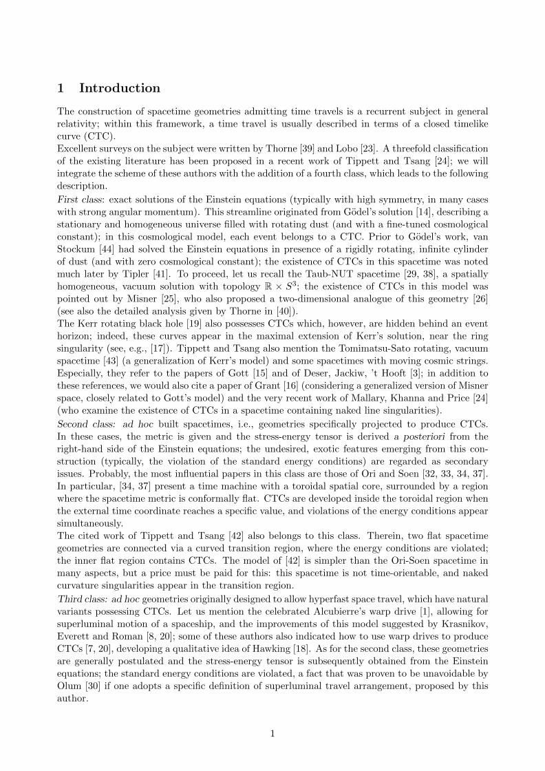
In each one of Eq.s (6.14)-(6.16), the terms in the right-hand sides have the following meaning:

- the terms in the first line of each equation are the contributions to t2/R, ϕ2 or τ2/R from thegeodesic motion in the spacetime region inside the smaller torus Tλ, where R− λ 6 ρ 6 R+ λ;

- the terms in the second lines of Eq.s (6.14) (6.16) and in the second and third lines of Eq. (6.15)are the contributions from the motion in the Minkowskian region outside the larger torus TΛ,where ρ 6 R− Λ or ρ > R+ Λ;

17

- the integrals occupying the third and fourth lines of Eq.s (6.14) (6.16) and the fourth and fifthlines of Eq. (6.15) are the contribution from the transition region where R − Λ < ρ < R − λor R + λ < ρ < R + Λ. Let us notice that all the contributions on the right-hand side of Eq.(6.16) are strictly positive. This indicates that the arrival proper time τ2 of the test particleis always positive, which correctly corresponds to the fact that we are using a future-orientedparametrization of the geodesic.

6.5 How to fulfil the previous claims about the time travel

Let us focus on the expression (6.14) for t2. The term in the first line of the cited equation (thecontribution from the region inside Tλ) is certainly negative, in agreement with the remarks madeafter Eq. (5.17); on the contrary, the term in the second line is positive, while the sign of the integralin the third and fourth lines is not evident a priori. The hope is to make the negative term verylarge and dominant on the others, by an appropriate choice of the parameters; this choice shouldinduce the claimed condition t2 < 0 of (6.11), corresponding to a time travel into the past. Thisgoal can be attained choosing the rescaled momentum ω so as to make very small the expressionwithin the square brackets in the first line of Eq. (6.14); we will analyse this strategy in greaterdetail in the forthcoming paragraph 6.5.1 and show that it allows to fulfil all claims of subsection6.3.Let us remark that, besides fulfilling t2 < 0, the parameters should also be tuned properly so thatϕ2 given by Eq. (6.15) is an integer multiple of 2π (see Eq. (6.12)). When this condition is realized,the test particle travelling along the geodesic returns exactly to the initial spatial position, fromwhich its journey had started.

6.5.1 Setting up the previous strategy

Following the previous idea, let us fix the attention on the variable

$ :=

√ω2 − a2

b2

(1 +

b2

γ2

)∈

0 ,

√(1− Λ

R

)2(1− 1

γ2

)− a2

b2

(1 +

b2

γ2

) (6.17)

which is (the square root of) the term between square brackets in the first line of Eq. (6.14) for t2.Our strategy is to make $ small.For definiteness, let us assume the shape function H = H(k) to have the form (A.3) (A.4) given inAppendix A for some finite integer k > 2.In Appendix B we illustrate a method for high precision calculation of t2/R, ϕ2 and τ2/R when $ issmall. This method uses directly the definitions (6.14)-(6.16) of these quantities; in particular, theintegrals appearing therein are re-expressed in a way which is more convenient for their numericalevaluation.Section B.2 of the above mentioned Appendix B also considers the limit

$ → 0+ (6.18)

and derives the expansions

t2R

= −(

4 a

b2λ

R

)1

$

(1 + O

($

2k+1))

; (6.19)

ϕ2 =

(4

b

λ

R

√1 +

b2

γ2

)1

$

(1 + O

($

2k+1))

; (6.20)

τ2

R=

(4 a

γ

λ

R

)1

$

(1 + O

($

2k+1))

. (6.21)

18

Let us briefly comment the above results.

- The asymptotic expansion (6.19) shows that t2 can be made negative, with |t2| arbitrarily large(one simply has to choose $ small enough).

- On the other hand, Eq. (6.20) shows that ϕ2 varies rapidly when $ is small, meaning that littlechanges of $ correspond to non-negligible deviations of ϕ2. This indicates that fulfilling thecondition ϕ2 = 0 (mod 2π) (see Eq. (6.12)) is always possible in principle, but requires a finetuning of the parameter $; the asymptotic expression (6.20) for ϕ2 is not sufficient to determinethis fine-tuned value of $ and it is necessary to use directly the exact expression (6.15).

- Finally, let us remark that the leading order in the asymptotic expansion (6.21) for τ2 is inverselyproportional to the Lorentz factor γ; in particular, by comparison with the expansion (6.19) we

see that τ2/|t2| = (b2/γ)(1 +O($

2k+1 )

). So, τ2 can be made small with respect to |t2| choosing a

large γ, exactly as in special relativity.

Summing up: with appropriate, small values of $ and sufficiently large γ we can fulfil all claims ofsubsection 6.3. In the next section we describe this situation via fully quantitative examples.

6.6 Some numerical examples

In this subsection we fix as follows the parameters of the problem and the shape function:

λ =3

5R , Λ =

4

5R , a =

9

100, b = 10 ;

H = H(k) as in Eq.s (A.3) (A.4) of Appendix A , k = 3 .

(6.22)

These choices determine the time machine up to the scale factor R, for which we will subsequentlyconsider different choices.Concerning the parameters of the geodesic motion, we set

ρ0 = (1 + 10−3) (R+ Λ) (6.23)

(meaning that, at τ = 0, the particle is outside but very close to the external torus TΛ). The otherparameters describing the particle motion are γ and $, defined by Eq. (6.17); they are free for themoment, but $ is assumed to be small.Due to Eq.s (6.17) (6.22) and (6.23), in the expressions (6.14)-(6.16) for t2, ϕ2, τ2 (as well as in theirsmall-$ asymptotic versions (6.19)-(6.21)) everything depends only on the scale parameter R ofthe time machine and on the kinematic parameters γ,$. In particular, the $ → 0+ asymptoticexpressions (6.19) and (6.21) become

t2R

= − 27

12500$

(1 +O

(√$))

, (6.24)

τ2

R=

27

125 γ $

(1 +O

(√$))

. (6.25)

We have checked that, ignoring the remainder terms O(√$), the above asymptotic expressions

agree up to 4 significant digits with the numerical values of the exact expressions (6.14)-(6.16) for$ ' 10−5; the agreement is even more accurate for smaller values of $.

As an example, let us choose R = 100m (' 100/(2.99792458 · 108) s in our units with c = 1); wewant to determine the remaining parameters γ,$ so that t2 ' −1 y and τ2 ' 1 d (y and d stand,respectively, for “year” and “day”). To this purpose, we first use the asymptotic expressions (6.24)(6.25) for a preliminary, rough estimate. From Eq. (6.24) we infer t2 ' −1 y if $ ' 2.28 · 10−17; on

19

TABLE 1 : R = 102m minEf = −1.2809... · 1023 gr/cm3

γ $ |ϕ2| (mod 2π) t2 τ2 maxα (g/m) minEg (gr/cm3)

1.1 7.2001167584668·10−10 2 · 10−5 −1 s 90.97 s 6.679 · 1016 −1.347 · 1023

102 7.2001526829246·10−10 6 · 10−7 −1 s 1 s 4.144 · 1017 −6.779 · 1025

102 2.280028356416717·10−17 10−6 −1 y 1 y 4.144 · 1017 −6.779 · 1025

104 2.280021827804094·10−17 10−6 −1 y 3.66 d 4.143 · 1021 −6.768 · 1029

105 2.280020685289079·10−20 3 · 10−6 −103 y 1 y 4.143 · 1023 −6.768 · 1031

107 2.280020673890116·10−20 5 · 10−6 −103 y 3.66 d 4.143 · 1027 −6.768 · 1035

108 2.2800206734492706·10−23 10−6 −106 y 1 y 4.143 · 1029 −6.768 · 1037

1010 2.2800206734492592·10−23 10−6 −106 y 3.66 d 4.143 · 1033 −6.768 · 1041

TABLE 2 : R = 1011m minEf = −1.2809... · 105 gr/cm3

γ $ |ϕ2| (mod 2π) t2 τ2 maxα (g/m) minEg (gr/cm3)

102 2.28000847482·10−8 4 · 10−6 −1 y 1 y 0.4144 −6.779 · 107

104 2.280027538409·10−8 4 · 10−7 −1 y 3.66 d 4.143 · 103 −6.768 · 1011

105 2.2800350451561739·10−11 3 · 10−6 −103 y 1 y 4.143 · 105 −6.768 · 1013

107 2.2800078145725598·10−11 4 · 10−6 −103 y 3.66 d 4.143 · 109 −6.768 · 1017

108 2.280021127512103772·10−14 7 · 10−6 −106 y 1 y 4.143 · 1011 −6.768 · 1019

1010 2.2800211275120923732·10−23 8 · 10−6 −106 y 3.66 d 4.143 · 1015 −6.768 · 1023

TABLE 3 : R = 1018m minEf = −1.2809... · 10−9 gr/cm3

γ $ |ϕ2| (mod 2π) t2 τ2 maxα (g/m) minEg (gr/cm3)

105 2.28157870976775·10−4 2 · 10−12 −925 y 1.02 y 4.143 · 10−9 −0.6778

107 2.28157869832448·10−4 3 · 10−12 −925 y 3.73 d 4.143 · 10−9 −6.778 · 103

108 2.280006782789627·10−7 2 · 10−10 −106 y 1 y 4.143 · 10−3 −6.768 · 105

109 2.280006782789616·10−7 2 · 10−10 −106 y 36.6 d 0.4143 −6.768 · 107

1010 2.280006782789615·10−7 4 · 10−10 −106 y 3.66 d 41.43 −6.768 · 109

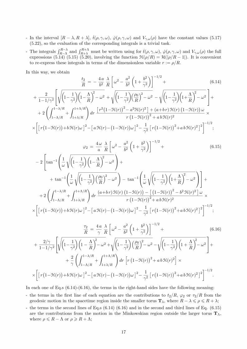
Tables 1-3: some numerical examples corresponding to the choices (6.22) for a, b,Λ/R, λ/R and H.The values of |ϕ2|, t2 and τ2 are computed via Eq.s (6.14)-(6.16) (in the reformulations of AppendixB); the value of maxα is obtained using Eq. (7.9), while those of min Ef and min Eg descend fromEq.s (8.8) and (8.11). (m := meter, cm := centimeter, gr := gram, s := second, d := day, y := year,g := Earth’s gravitational acceleration).

the other hand, keeping this choice of $, Eq. (6.25) gives τ2 ' 1 d for γ ' 104. Then, we fix γ = 104

and consider small variations of $ about the value 2.28 · 10−17 to get ϕ2 ' 0 (mod 2π); using Eq.(6.15), we find that |ϕ2| < 10−6 (mod 2π) if we use the fine-tuned value $ = 2.280021827804094 ·10−17. From the previous values of R, γ,$ and from the exact expressions (6.14) (6.16) we gett2 = −1.002... y and τ2 = 3.657... d (indeed, for these calculations Eq.s (6.14)-(6.16) are used inthe reformulations described in Appendix B, more suitable for precise numerical evaluation of theintegrals therein).In the first five columns of Tables 1-3 we summarize the above results and many others, obtainedalong the same lines using (Eq.s (6.24) (6.25) and) Eq.s (6.14)-(6.16); the parts of the tables contain-ing the symbols α, Ef and Eg refer to the tidal accelerations and energy densities already mentionedin the introduction, and will be explained in the forthcoming Sections 7 and 8. Concerning thevalues of R chosen in the said tables, we note that 1011m is the order of magnitude of the Earth-Sundistance, while 1018m ' 100 light years: this is the choice yielding the smallest values for the tidalaccelerations and the energy densities.

20

7 Tidal accelerations

In this section we give a quantitative analysis of the tidal accelerations experienced by small extendedbodies during free fall time travels into the past; we assume that during such trips, the particlesconstituting these bodies move along geodesics of the type analysed in Section 6.To introduce the subject, it is convenient to start with some general facts.

7.1 Basics on tidal effects

Let us consider an arbitrary spacetime M with metric g, and a timelike geodesic with its propertime parametrization ξ : I ⊂ R→M, τ 7→ ξ(τ). For each τ ∈ I, we introduce the vector space

Sτ :=X ∈ Tξ(τ)M

∣∣ g(X, ξ(τ))

= 0

(7.1)

and the linear operator

Aτ : Sτ → Sτ , X 7→ AτX := −Riem(X, ξ(τ)

)ξ(τ) (7.2)

where Riem denotes the Riemann curvature tensor. It can be easily checked that Sτ is a 3-dimensional, spacelike linear subspace of the tangent space Tξ(τ)M; with the restriction of g ≡ gξ(τ)

as an inner product, Sτ is in fact a Euclidean space. Aτ is a self-adjoint linear operator in thisEuclidean space (and thus it is diagonalizable, with real eigenvalues).We refer to Aτ as the tidal operator for the geodesic ξ at τ . This name is due to the following fact:if we consider another timelike geodesic “infinitesimally close to ξ” and δξ(τ) ∈ Sτ is its infinitesimalseparation vector from ξ(τ), the tidal acceleration (∇2δξ/dτ2)(τ) equals Aτ δξ(τ). Of course, ξ andξ + δξ could be the worldlines of two particles in a freely falling extended body.For a justification of all the previous statements about Sτ and Aτ , we refer to Appendix C. In thesequel we consider the scalar quantity

α(τ) := supX∈Sτ\0

√g(AτX,AτX)√g(X,X)

, (7.3)

which is just the operator norm of Aτ corresponding to the Euclidean norm√g( · , · ) ≡

√gξ(τ)( · , · )

on Sτ . By the spectral theorem for self-adjoint operators, the above sup equals the maximum of theabsolute values of the eigenvalues of Aτ , and it is attained when X is an associated eigenvector.For obvious reasons, we shall call α(τ) the maximal tidal acceleration per unit length. Let us remarkthat, if a timelike geodesic has a separation δξ from ξ, the tidal acceleration at τ associated to ithas norm √

g(Aτδξ(τ),Aτδξ(τ)

)6 α(τ)

√g(δξ(τ), δξ(τ)

); (7.4)

the above relation holds as an equality if δξ(τ) is an eigenvector associated to an eigenvalue of Aτwith maximum absolute value.

7.2 Tidal effects during time travel

Let us return to the spacetime T and choose for ξ a timelike geodesic of the type considered inSection 6, describing a time travel by free fall. A sketch of the computation of Aτ and α(τ) for thiscase is given in Section C.2 of Appendix C; therein we write

Aτ =γ2

R2Aτ (7.5)

21

1- /R

1- /R 1+ /R

1+ /R

1 2r0

2.×104

4.×104

6.×104

8.×104

a

Figure 4a

1- /R

1- /R 1+ /R

1+ /R

1 2r0

10

20

30

40

50

a

Figure 4b

Figures 4a-4b: graphs of the function r 7→ a(r) for λ/R = 3/5, Λ/R = 4/5, a = 9/100, b = 10 and for γ = 1.1,

$ = 7.2... ·10−10 (case (a)) or in the limit γ → +∞, $ → 0+ (case (b)). Again, the shape function H = H(k)

is the one given in Eq.s (A.3) (A.4) of Appendix A, with k = 3.

with Aτ : Sτ → Sτ self-adjoint, and show that

α(τ) =γ2

R2a(ρ(τ)/R

), (7.6)

where a(r) is a dimensionless function of a variable r ∈ (0,+∞), here set equal to ρ(τ)/R; this func-tion also depends, parametrically, on the quantities λ/R,Λ/R, a, b and γ,$ (related, respectively,to the metric g and to the motion ξ). The function a(r) can be computed explicitly and vanishesidentically for r outside the region (1−Λ/R, 1−λ/R)∪(1+λ/R, 1+Λ/R) (because the Riemanniancurvature is zero for ρ/R outside this region).In the simultaneous limits γ → +∞ and $ → 0+, Aτ has a zero eigenvalue of multiplicity 2 and asimple, non-zero eigenvalue depending only on r = ρ(τ)/R; the explicit expression of this eigenvalueis reported in Appendix C (see Eq. (C.13) therein) and the corresponding eigenvector, giving thedirection of the tidal acceleration, is ∂z

∣∣ξ(τ)

. Of course the function r 7→ a(r) has a limit for γ → +∞and $ → 0+, coinciding with the absolute value of this eigenvalue.For a better quantitative appreciation, it is convenient to express α(τ) in terms of the ratio g/mwhere (m := meter and) we are considering the nominal Earth’s gravitational acceleration

g := 9.8 m/s2 = 1.090397... · 10−16m−1 (7.7)

(the last equality follows from our convention c = 1).Eq.s (7.6) and (7.7) imply

α(τ) =(9.170971... · 1015

) γ2

(R/m)2a(ρ(τ)/R

) gm

. (7.8)

From here to the end of this subsection we fix λ/R,Λ/R, a, b and H = H(k) as in Eq. (6.22). Fig.s4a-4b show the graphs of the function r 7→ a(r) for a specific choice of (γ,$) or for γ → +∞,$ → 0+. The sixth columns of Tables 1-3 give for some choices of R, γ,$ the maxima of α duringthe time travel, i.e.,

maxα := maxτ∈[0,τ2]

α(τ) =(9.170971... · 1015

) γ2

(R/m)2

(max

r∈[ρ0/R,ρ1/R]a(r)

)gm

. (7.9)

Finally, let us remark that Table 3 indicates a fact already anticipated in paragraph 6.6: for R =1018m ' 100 light years, the tidal accelerations per unit length are gentle (on a human scale) up tovery large values of γ (say, up to γ = 109).

22

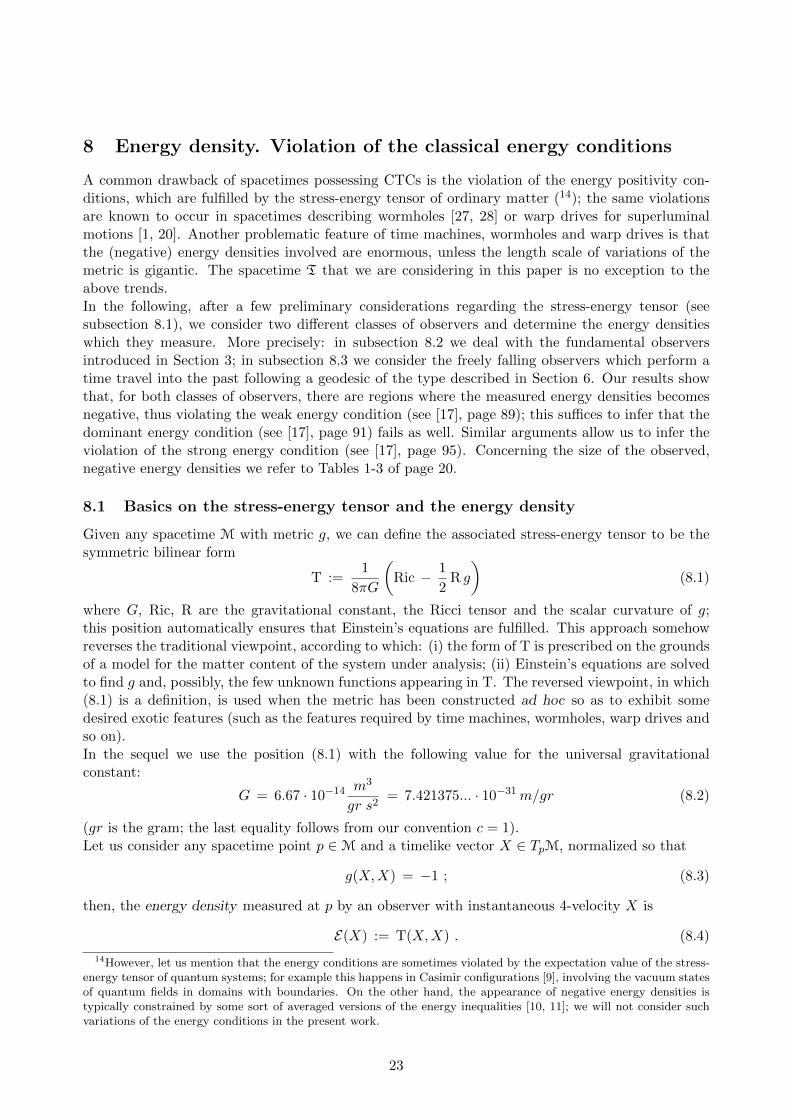
8 Energy density. Violation of the classical energy conditions

A common drawback of spacetimes possessing CTCs is the violation of the energy positivity con-ditions, which are fulfilled by the stress-energy tensor of ordinary matter (14); the same violationsare known to occur in spacetimes describing wormholes [27, 28] or warp drives for superluminalmotions [1, 20]. Another problematic feature of time machines, wormholes and warp drives is thatthe (negative) energy densities involved are enormous, unless the length scale of variations of themetric is gigantic. The spacetime T that we are considering in this paper is no exception to theabove trends.In the following, after a few preliminary considerations regarding the stress-energy tensor (seesubsection 8.1), we consider two different classes of observers and determine the energy densitieswhich they measure. More precisely: in subsection 8.2 we deal with the fundamental observersintroduced in Section 3; in subsection 8.3 we consider the freely falling observers which perform atime travel into the past following a geodesic of the type described in Section 6. Our results showthat, for both classes of observers, there are regions where the measured energy densities becomesnegative, thus violating the weak energy condition (see [17], page 89); this suffices to infer that thedominant energy condition (see [17], page 91) fails as well. Similar arguments allow us to infer theviolation of the strong energy condition (see [17], page 95). Concerning the size of the observed,negative energy densities we refer to Tables 1-3 of page 20.

8.1 Basics on the stress-energy tensor and the energy density

Given any spacetime M with metric g, we can define the associated stress-energy tensor to be thesymmetric bilinear form

T :=1

8πG

(Ric − 1

2R g

)(8.1)

where G, Ric, R are the gravitational constant, the Ricci tensor and the scalar curvature of g;this position automatically ensures that Einstein’s equations are fulfilled. This approach somehowreverses the traditional viewpoint, according to which: (i) the form of T is prescribed on the groundsof a model for the matter content of the system under analysis; (ii) Einstein’s equations are solvedto find g and, possibly, the few unknown functions appearing in T. The reversed viewpoint, in which(8.1) is a definition, is used when the metric has been constructed ad hoc so as to exhibit somedesired exotic features (such as the features required by time machines, wormholes, warp drives andso on).In the sequel we use the position (8.1) with the following value for the universal gravitationalconstant:

G = 6.67 · 10−14 m3

gr s2= 7.421375... · 10−31m/gr (8.2)

(gr is the gram; the last equality follows from our convention c = 1).Let us consider any spacetime point p ∈M and a timelike vector X ∈ TpM, normalized so that

g(X,X) = −1 ; (8.3)

then, the energy density measured at p by an observer with instantaneous 4-velocity X is

E(X) := T(X,X) . (8.4)

14However, let us mention that the energy conditions are sometimes violated by the expectation value of the stress-energy tensor of quantum systems; for example this happens in Casimir configurations [9], involving the vacuum statesof quantum fields in domains with boundaries. On the other hand, the appearance of negative energy densities istypically constrained by some sort of averaged versions of the energy inequalities [10, 11]; we will not consider suchvariations of the energy conditions in the present work.

23

Figure 5a

1- /R

1- /R 1+ /R

1+ /R

1 2r0

-1.×104

-2.×104

-3.×104

f

Figure 5b

Figures 5a-5b: density plot of the function (r, ζ) 7→ Ef (r, ζ) and graph of the function r 7→ Ef (r, 0), for

λ/R = 3/5, Λ/R = 4/5, a = 9/100, b = 10. Again, the shape function H = H(k) is the one given in Eq.s

(A.3) (A.4) of Appendix A, with k = 3.

Let us mention that, with the present notations, the weak energy condition reads E(X) > 0 for eachX as above.From now on, M is the spacetime T of the present paper; Appendix D gives some information onthe calculation of T in this case. We will consider two choices for the vector X, corresponding to theobservers already mentioned at the beginning of the present section. Using the fact that energiesand masses are dimensionally equivalent in our setting with c = 1, we will measure energy densitiesin units of gr/cm3.

8.2 The energy density measured by fundamental observers

Let us consider the fundamental observer passing through a spacetime point p ∈ T, and rememberthat its four-velocity coincides with E(0)(p) (here and in the following E(0) is the timelike vectorfield in the tetrad of Section 3). Consequently, the energy density measured by this observer is

Ef (p) := E(E(0)(p)

). (8.5)

The above function of p depends on its coordinates ρ, z in the following way:

Ef =1

8πGR2Ef (ρ/R, z/R) =

5.361369... · 1022

(R/m)2Ef(ρ/R, z/R

) gr

cm3, (8.6)

for a suitable, dimensionless function Ef of two variables r, ζ (here set equal to ρ/R, z/R), whichalso depends on the parameters λ/R,Λ/R, a, b and on the shape function H. The second equality inEq. (8.6) follows from Eq. (8.2) for G. The function Ef can be computed analytically and vanishes

identically for√

(r − 1)2 + ζ2 ∈ [0, λ/R] ∪ [Λ/R,+∞) (i.e., where the curvature is zero). Furtherdetails on this topic can be found in Appendix D.For an appreciation of the above statements, let us fix λ/R,Λ/R, a, b and H = H(k) as in Eq. (6.22);for these choices, Figure 5a describes Ef as a function of the variables r = ρ/R, ζ = z/R and Figure5b is the graph of the function r 7→ Ef (r, 0).

24

1- /R

1- /R 1+ /R

1+ /R

1 2r0

-3.×104

-2.×104

-1.×104

g

Figure 6a

1- /R

1- /R 1+ /R

1+ /R

1 2r0

-1.5×103

-1.×103

-5.×102

5.×102

1.×103

g

Figure 6b

Figures 6a-6b: graphs of the function r 7→ Eg(r) for λ/R = 3/5, Λ/R = 4/5, a = 9/100, b = 10 and for

γ = 1.1, $ = 7.2... · 10−10 (Fig. 6a), or in the limit γ → +∞, $ → 0+ (Fig. 6b). Again, the shape function

H = H(k) is the one given in Eq.s (A.3) (A.4) of Appendix A, with k = 3.

A look at Figure 5b suffices to realize that Ef attains negative values; so, the weak energy conditionE(X) > 0 fails for X = E(0)(p) at suitable points p ∈ T. With our choices (6.22), Ef is a boundedfunction of (r, ζ) with absolute minimum

minEf = Ef (1.691442... , 0) = − 2.389140... · 104 . (8.7)

Using the above numerical value for the minimum, we infer from (8.6) that

min Ef = − 1.280906... · 1027

(R/m)2

gr

cm3(8.8)

The outcomes of this formula for some values of R are given in Tables 1-3 of page 20. In passing,we remark that all the values of |min Ef | arising from the cited tables are considerably smaller thanthe Planck density ρP := c5/(~G2) = 5.155... · 1093gr/cm3 (~ is the reduced Planck constant); so,no quantum gravity effect seems to be involved in the physical regimes described by the tables. Forthe specific value R = 1018m ' 100 light years, |min Ef | is indeed much smaller than 1gr/cm3.

8.3 The energy density measured during time travel

Let us now pass to determine the energy density measured by a freely falling observer who performsa time travel into the past, moving along a timelike geodesic ξ of the type analysed in Section 6. Atproper time τ , this observer has four-velocity ξ(τ) ∈ Tξ(τ)T and measures the energy density

Eg(τ) := E(ξ(τ)

); (8.9)

indicating with ρ(τ) the radial coordinate of ξ(τ), we find

Eg(τ) =γ2

8πGR2Eg(ρ(τ)/R

)=

(5.361369... · 1022

)γ2

(R/m)2Eg(ρ/R

) gr

cm3, (8.10)

where the second identity follows again from Eq. (8.2), and Eg is a suitable, dimensionless functionof the variable r = ρ(τ)/R which also depends on the parameters λ/R,Λ/R, a, b and γ,$ (related,respectively, to the metric g and to the geodesic ξ). The function Eg(r) can be computed explicitlyand vanishes identically for r outside the region (1 − Λ/R, 1 − λ/R) ∪ (1 + λ/R, 1 + Λ/R) (wherethe curvature is zero); moreover, it has a limit for γ → +∞ and $ → 0, simultaneously.Again, let us fix λ/R,Λ/R, a, b and H = H(k) as in Eq. (6.22). Fig.s 6a-6b show the graphs of thefunction r 7→ Eg(r) for a particular choice of (γ,$) or for γ → +∞, $ → 0+; from these graphs,

25

it can be readily inferred that in general Eg is not positive, thus proving that the weak energycondition E(X) > 0 is violated for X = ξ(τ) and for suitable values of the proper time τ . Let usconsider the absolute minimum of Eg along the travel, i.e.,

min Eg := minτ∈[0,τ2]

Eg(τ) =

(5.361369... · 1022

)γ2

(R/m)2

(min

r∈[ρ0/R,ρ1/R]Eg(r)

)gr

cm3; (8.11)

note that the minimum of Eg depends on the parameters γ,$. The last columns of Tables 1-3 onpage 20 give the numerical value of min Eg, descending from Eq. (8.11), for some choices of R, γ,$;these minima appear to be much smaller than the Planck density (so we can repeat the commentsat the end of the previous subsection).Finally, let us remark that for R = 1018m ' 100 light years, the energy density measured by a freelyfalling time traveller has an absolute value . 1 gr/cm3 even for the quite large choice γ = 105.

Acknowledgments. This work was supported by: INdAM, Gruppo Nazionale per la Fisica Matem-atica; INFN; MIUR, PRIN 2010 Research Project “Geometric and analytic theory of Hamiltoniansystems in finite and infinite dimensions”; Universita degli Studi di Milano.We wish to thank Prof. Ori and the anonymous referees for valuable suggestions and bibliographicalindications which helped improving the quality of the manuscript.

26

A Appendix. On the shape function HLet us make reference to the framework of Section 2 and recall that the basic function X , whichdetermines the line element ds2 of Eq. (2.5), is defined in terms of a suitable, auxiliary shapefunction H ∈ Ck([0,+∞)) (k ∈ 2, 3, ...,∞). In the present appendix we provide explicit examplesH(k) of admissible choices of H for any k ∈ 0, 1, ...,∞ (15), fulfilling the requirement (2.4) reportedhereafter:

H(y) = 1 for y ∈ [0, λ/R] , H(y) = 0 for y ∈ [Λ/R,+∞) .

In the two forthcoming paragraphs, we discuss separately the cases with k > 0 finite and the casek = +∞.

An admissible choice H = H(k) ∈ Ck([0,+∞)), for k >>> 0 finite. Let us first consider thefunction

h(k)(v) :=

vk (1− v)k for v ∈ [0, 1] ,

0 for v ∈ (−∞, 0] ∪ [1,+∞) .(A.1)

Notice that the function h(0), corresponding to k = 0, is piecewise constant and discontinuous; on

the other hand, we have h(k) ∈ Ck−1(R) for all k > 1.Next, we introduce the normalized primitive of h(k) given by

H(k)(w) :=

(∫ +∞

−∞dv h(k)(v)

)−1 ∫ w

−∞dv h(k)(v) (w ∈ R) . (A.2)

In view of the previous considerations on the regularity of h(k), it can be readily inferred that

H(k) ∈ Ck(R). Furthermore, let us stress that it is possible to derive an explicit, piecewise polynomialexpression for H(k); more precisely, taking into account the definition (A.1) of h(k) and using someknown relations for the incomplete beta function (see, e.g., Eq.s 8.17.1, 8.17.2 and 8.17.5 on page183 of [31]), it can be proved by simple computations that

H(k)(w) =

0 for w ∈ (−∞, 0] ,

k∑j=0

(2k+1

j+k+1

)wj+k+1 (1− w)k−j for w ∈ [0, 1] ,

1 for w ∈ [1,+∞) .

(A.3)

Finally, we set

H(k)(y) := H(k)

(Λ/R− y

Λ/R− λ/R

)for y ∈ [0,+∞) . (A.4)

The previous considerations ensure that H(k) is of class Ck and even fulfils the requirement (2.4),thus determining an admissible choice of H.

An admissible choice H = H(∞) ∈ C∞([0,+∞)). In this case we can follow the same stepsdescribed in the previous paragraph, starting with the smooth function

h(∞)(v) :=

e− 1v(1−v) for v ∈ [0, 1] ,

0 for v ∈ (−∞, 0] ∪ [1,+∞) .(A.5)

15Notice that the stricter assumption k > 2 made in Section 2 (and adhered to throughout all the paper) is motivatedby the will to avoid the appearance of curvature singularities; for the purposes of this appendix, that assumption canbe generalized requiring k > 0.

27

Using the above function, we can proceed to introduce a map H(∞) by a definition analogous to(A.2); more precisely, we set

H(∞)(w) :=

(∫ +∞

−∞dv h(∞)(v)

)−1 ∫ w

−∞dv h(∞)(v) (w ∈ R) . (A.6)

This function is itself smooth and fulfils, in addition, (16)

H(∞)(w) = 0 for w ∈ (−∞, 0] , H(∞)(w) = 1 for w ∈ [1,+∞) . (A.7)

In conclusion, similarly to what we did in the preceding paragraph for k > 0 finite, we determinean admissible, smooth choice of H fulfilling Eq. (2.4) with the position

H(∞)(y) := H(∞)

(Λ/R− y

Λ/R− λ/R

)for y ∈ [0,+∞) . (A.8)

A final remark. The functions h(k), h(∞) of Eq.s (A.1), (A.5) are positive on (0, 1). Due to this,the normalized primitives H(k), H(∞) of Eq.s (A.2), (A.6) are strictly increasing on (0, 1). Thereforethe functions H(k), H(∞) of Eq.s (A.4), (A.8) are strictly decreasing on (λ/R,Λ/R), i.e., they fulfilcondition (2.11).

B Appendix. A class of integrals depending on a parameter. Ap-plications to the integrals in Eq.s (6.14)-(6.16)

In the present appendix we report a number of results about a class of integrals depending on aparameter, focusing especially on their evaluation for small values of the parameter. These resultsallow us, in particular, to treat the integrals appearing in Eq.s (6.14)-(6.16) of subsection 6.5, in allthe cases of interest for the applications discussed therein.In the forthcoming subsection B.1 we show that, by means of simple changes of variables, the studyof all the above cited integrals can be reduced to the analysis of a general class of integrals J(ε),depending on a small parameter ε. In the following subsection B.2 we derive a preliminary boundfor J(ε) holding for all ε > 0, which provides a control of its singular behaviour for ε → 0+. Insubsection B.3 we determine an alternative representation for J(ε), allowing to cure some difficultieswhich arise in the numerical evaluation for small ε (this is an essential result for the applications ofsubsections 6.5, 6.6). In the conclusive subsection B.4 we use this alternative representation of J(ε)to determine its leading-order contributions for ε→ 0+.

B.1 The general structure for the integrals in Eq.s (6.14)-(6.16)

Let us consider the integral expressions appearing in Eq.s (6.14)-(6.16) and recall that, for theapplications discussed in subsections 6.5 and 6.6, it is of interest to evaluate them when (see Eq.s(6.4), (6.17) and (6.18))

ω =

√a2

b2

(1 +

b2

γ2

)+$2 and 0 < $ 1 .

Assuming the shape function H = H(k) has the form (A.3) (A.4) given in Appendix A for somefinite k > 2 and making the change of variables

v :=

r − 1 + Λ/R

Λ/R− λ/Rfor r ∈

(1− Λ

R, 1− λ

R

),

r − 1− λ/RΛ/R− λ/R

for r ∈(

1 +λ

R, 1 +

Λ

R

) ς := b2$2 , (B.1)

16Even though in this case it is not possible to derive a fully explicit expression for H(∞) in terms of elementary (orspecial) functions, one can use directly the integral representation (A.6) for the numerical computations of interest inthe applications.

28

all the integrals mentioned above can be written in the following form:

I(ς) :=

∫ 1

0dv

P(v, ς)√ς + vhQ(v, ς)

, (B.2)

where ς ∈ (0, ς∗) for some ς∗ > 0 (see Eq.s (6.17) (B.1)), h := k + 1 > 3, P,Q ∈ C∞([0, 1]× [0, ς∗])(17) and

ς + vhQ(v, ς) > 0 for all (v, ς) ∈([0, 1]×[0, ς∗]

)\(0, 0) ,

Q0 := Q(0, 0) > 0 .(B.3)

The rest of this appendix is devoted to the analysis of any integral of this form, with h ∈ 3, 4, 5, ...(18). To this purpose, it is convenient to introduce the rescaled parameter

ε := (ς/Q0)1/h ∈(0, ε∗

), ε∗ := (ς∗/Q0)1/h (B.4)

and use it to re-express Eq. (B.2) as

I(ς) = J((ς/Q0)1/h

), J(ε) :=

1√Q0

∫ 1

0dv

P(v,Q0 εh)√

εh + vhQ(v,Q0 εh)/Q0

. (B.5)

As previously hinted at, our main concern is the investigation of the asymptotic behaviour of J(ε)for ε→ 0+. Let us notice that the integrand function in Eq. (B.5) evaluated at ε = 0 diverges in anon-integrable way for v→ 0+; this suggests that J(ε) should become singular for ε→ 0+.

B.2 A preliminary bound for J(ε)

Keeping in mind the definition (B.5) of J(ε), let us consider the function

F(v, ε) :=P(v,Q0 ε

h)√εh + vh

√Q0

√εh + vhQ(v,Q0 εh)/Q0

. (B.6)

In view of the regularity features enjoyed by P and Q, we can readily infer that F(v, ε) is smoothon([0, 1]×[0, ε∗]

)\(0, 0); on the other hand, it can be proved that F has a continuous extension

to the origin (19). Thus we can regard F as a continuous function on [0, 1]×[0, ε∗], and

‖F‖C0 := sup(v,ε)∈ [0,1]×[0,ε∗]

∣∣F(v, ε)∣∣ < +∞ . (B.7)

17As a matter of fact, for the analysis discussed in the following it would suffice to assume that P,Q ∈C [(h+3)/2]([0, 1] × [0, ς∗]), where [(h + 3)/2] denotes the integer part of (h + 3)/2. However, for the cases of inter-est to us, actually both P and Q are smooth functions; more precisely, they are polynomials with respect to the firstvariable v (or ratios of polynomials with non-vanishing denominators), with coefficients depending smoothly on ς.

18Apart from the fact that in all the applications of interest in this work there holds h > 3, let us point out forcompleteness that the analysis of the cases where h = 1, 2 would actually require a separate treatment, involvingslightly different computations.

19To prove this claim, let us consider on R2 the norm ‖(v, ε)‖h := (|v|h+ |ε|h)1/h (recall that all norms on R2 areequivalent, since we have a finite-dimensional vector space). Then, on account of the fact that P,Q ∈ C∞([0, 1]×[0, ς∗])(so that, in particular, P,Q ∈ C1([0, 1] × [0, ς∗]) ), we have P(v, ε) = P(0, 0) + O(‖(v, ε)‖h) and Q(v, ε)/Q0 =1 +O(‖(v, ε)‖h) for (v, ε)→ (0, 0); in the same limit, it is vh = O(‖(v, ε)‖hh). Recalling the definition (B.6) of F , theprevious considerations allow us to infer by simple computations that

F(v, ε) =P(0, 0) +O(‖(v, ε)‖h)√Q0

√1 + O(‖(v, ε)‖h)

=P(0, 0)√Q0

+O(‖(v, ε)‖h) ;

thus, we can extend continuously F to the origin setting F(0, 0) := P(0, 0)/√Q0 .

29

Now, from the definition (B.5) of J(ε) we infer the bound∣∣J(ε)∣∣ =

∣∣∣∣ ∫ 1

0dv

F(v, ε)√εh + vh

∣∣∣∣ 6 ‖F‖C0

∫ 1

0dv

1√εh + vh

. (B.8)

On the other hand, for any 0< ε < 1 we have the following chain of elementary estimates (recallthat we are assuming h > 3):∫ 1

0dv

1√εh + vh

6∫ ε

0dv

1√εh

+

∫ 1

εdv

1√vh

6h

h− 2

1

εh/2−1. (B.9)

Summing up Eq.s (B.6)-(B.9) show that, if ε∗ < 1,∣∣J(ε)∣∣ 6 (

h

h− 2‖F‖C0

)1

εh/2−1for all ε ∈

(0, ε∗

]. (B.10)

B.3 An alternative representation of J(ε)

In the applications considered in this work, it is often of interest to determine with great accuracythe numerical value of integrals such as J(ε) for small values of the parameter ε. This task is plaguedby unpleasant numerical instabilities, which can be ascribed to the singular behaviour of J(ε) forε→ 0+. In the following we shall derive an alternative representation for J(ε), isolating the leadingorder contributions which become singular for ε → 0+; this representation allows to perform thenumerical evaluation of J(ε) with greater efficiency and better accuracy.

To begin with, let us consider the integral J(ε) defined in Eq. (B.5); making the change of variablew := v/ε ∈ (0, 1/ε), by simple manipulations we obtain

J(ε) =

∫ 1/ε

0dw G(w, ε) , (B.11)

where we have set

G(w, ε) :=1

εh/2−1√Q0

√1 + wh

P(εw,Q0 εh)√

1 + wh

1+wh

(Q(εw,Q0 εh)

Q0− 1) . (B.12)

Recalling the regularity assumptions on P and Q, we can proceed to compute the Taylor expansionof G(w, ε) for ε→ 0+ up to order ε. To this purpose, it is useful to notice that

P(εw,Q0 εh) =

[(h+1)/2]∑n=0

1

n!(∂n1P)(0, 0) (εw)n + O

(ε[(h+3)/2]

)for ε→ 0+ ; (B.13)

of course, an analogous relation holds as well for Q. By a few additional computations, we obtain

G(w, ε) =1

εh/2−1√

1 + wh

[(h+1)/2]∑m,n=0

gm,n

(wh

1 + wh

)m(εw)n + O

(ε[(h+3)/2]

), (B.14)

where, the coefficients gm,n are completely determined by the values at the origin of P,Q and oftheir derivatives with respect to the first variable up to [(h+ 1)/2]-th order. For subsequent use, wedefine a reminder K[(h+1)/2] ∈ C0([0, 1/ε]× [0, (ς∗/Q0)1/h]) via the equation

K[(h+1)/2](w, ε) := G(w, ε) − 1

εh/2−1√

1 + wh

[(h+1)/2]∑m,n=0

gm,n

(wh

1 + wh

)m(εw)n . (B.15)

30

Thus, Eq.s (B.11), (B.14) and (B.15) give

J(ε) =

[(h+1)/2]∑m,n=0

gm,n jm,n(ε) + K[(h+1)/2](ε) , (B.16)

where we introduced the functions

jm,n(ε) :=1

εh/2−1−n

∫ 1/ε

0dw

whm+n

(1 + wh)m+1/2, (B.17)

K[(h+1)/2](ε) :=

∫ 1/ε

0dw K[(h+1)/2](w, ε) . (B.18)

Concerning the terms jm,n(ε), making the change of variable u := εhwh we obtain an integralcoinciding with the well-known representation for a Gaussian hypergeometric function 2F1 (see,e.g., Eq. (10) on page 59 of [6]); taking this into account, we get

jm,n(ε) =1

(hm+n+1) εh(m+1/2) 2F1

(m+

1

2, m+

n+1

h; m+

n+1

h+1 ; − 1

εh

). (B.19)

In passing, let us point out that the above result can be re-expressed as follows, for all h > 3 andn ∈ 0, ..., [(h+ 1)/2] such that (n+ 1)/h− 1/2 /∈ 0, 1, 2, ... (see Eq. (18) on page 63 and Eq. (2)on page 56 of [6]):

jm,n(ε) =

Γ(m+ n+1h ) Γ(1

2−n+1h )

hΓ(m+ 12)

1

εh2−1−n

+1

n+1− h2

2F1

(m+

1

2,

1

2−n+1

h;

3

2−n+1

h;− εh

).

(B.20)

As for the remainder K[(h+1)/2], we can return to the integration variable v = εw ∈ (0, 1); this gives

K[(h+1)/2](ε) =

∫ 1

0dv

1

εK[(h+1)/2](v/ε, ε) . (B.21)

The map (v, ε) 7→ (1/ε)K[(h+1)/2](v/ε, ε) is defined in principle on [0, 1] × (0, ε∗]; however, in allcases of interest in this work it has a continuous extension to [0, 1]× [0, ε∗] (20); this allows us to inferby Lebesgue’s dominated convergence that K[(h+1)/2](ε) has a continuous extension to ε = 0. Thecomputation of the reminder (B.21) is numerically stable due to the above mentioned continuityfeatures.In conclusion, Eq.s (B.14)-(B.21) give the alternative representation of J(ε) mentioned at the be-ginning of this subsection. This has been used to compute the integrals in Eq.s (6.14)-(6.16) for thevalues of the parameters reported in Tables 1-3; in this case, ε is proportional to $1/2.

B.4 Asymptotic expansion of J(ε) for ε→ 0+

The alternative representation (B.14)-(B.21) of J(ε) discussed in the previous subsection can beused to determine the leading-order, contributions to J(ε) for ε→ 0+; hereafter we shall give moredetails on this topic.

20Moreover, in all cases of interest for us one has

lim(v,ε)→(0+,0+)

(1

εK[(h+1)/2](v/ε, ε)

)= 0 .

31

First of all, let us investigate the asymptotic behaviour of the functions jm,n(ε) for ε → 0+; thisamounts to determine the leading order terms in the Gaussian hypergeometric function 2F1 appear-ing in Eq. (B.19). To this purpose, we follow the analysis reported in the paragraph 2.1.4 of [6].Let us notice that, in principle, the cases where (n+1)/h−1/2 is either in 0, 1, 2, ... or not must betreated separately. Since we have h > 3 and n ∈ 0, ..., [(h+ 1)/2] (see Eq. (B.16)), the condition(n+ 1)/h− 1/2 ∈ 0, 1, 2, ... is fulfilled only if h is even and n = [(h− 1)/2] = h/2− 1; in this case,we can use Eq. (18) on page 63 of [6] (along with some known identities for the digamma functionψ; see, e.g., Eq.s 5.4.12 and 5.4.15 on page 137 of [31]) to infer the identity

jm,h2−1(ε) = − ln ε+

2

h

(ln 2−

m∑`=1

1

2`− 1

) (h even

). (B.22)

In all the remaining cases where (n+ 1)/h− 1/2 /∈ 0, 1, 2, ... (i.e., for h even and n ∈ 0, ..., h/2−2∪h/2, or for h odd and n ∈ 0, ..., (h+1)/2), we can use the representation (B.20) of jm,n andthe series representation of the Gaussian hypergeometric function 2F1 (see, e.g., Eq. (2) on page 56of [6]) to obtain

jm,n(ε) =Γ(m+ n+1

h ) Γ(12 −

n+1h )

hΓ(m+ 12)

εn

εh/2−1+

1

n+ 1− h+ O

(εh)

for ε→ 0+ . (B.23)

Next, let us proceed to analyse the remainder term K[(h+1)/2](ε). Let us assume that the map(v, ε) 7→ (1/ε)K[(h+1)/2](v/ε, ε) has a continuous extension to [0, 1] × [0, ε∗] (see the comments onthis after Eq. (B.21)); then, we can introduce the continuous function

%[(h+1)/2](v) := limε→0+

(1

εK[(h+1)/2](v/ε, ε)

) (v ∈ [0, 1]

); (B.24)

and infer (again, by dominated convergence theorem) that

K[(h+1)/2](0) := limε→0+

K[(h+1)/2](ε) =

∫ 1

0dv %[(h+1)/2](v) < +∞ . (B.25)

Summing up, the above arguments yield the following asymptotic expansions for ε→ 0+:i) for h even, there holds

J(ε) =1

εh2−1

h2−2∑

n=0

h2∑

m=0

Γ(m+ n+1h ) Γ(1

2−n+1h )

hΓ(m+ 12)

gm,n

εn − h

2∑m=0

gm,h2−1

ln ε +

−

h2∑

m=0

h2−2∑

n=0

gm,n

h−1−n+

2

h

(m∑`=1

1

2`−1− ln 2

)gm,h

2−1 +

2 gm,h2

h−2

+ Kh2(0) + o(1) ;

(B.26)

ii) for h odd, there holds

J(ε) =1

εh2−1

h−32∑

n=0

h+12∑

m=0

Γ(m+ n+1h ) Γ(1

2 −n+1h )

hΓ(m+ 12)

gm,n

εn +

−

h+12∑

m,n=0

gm,n

h−1−n+ Kh+1

2(0) + o(1) .

(B.27)

32

C Appendix. On tidal accelerations

C.1 General facts

Our present aim is to account for all statements of subsection 7.1 on the grounds of well knownfacts.Given an arbitrary spacetime M, with metric g, we consider a timelike geodesic with a proper timeparametrization ξ : I → M, τ 7→ ξ(τ) (I ⊂ R an interval). We also introduce a variation of thisparametrized geodesic: by this we mean a (regular) family of maps ξσ : Iσ →M (σ ∈ (−ε, ε), Iσ⊂Ran interval) such that, for each σ, the map ξσ is a timelike geodesic in a proper time parametrizationand I0 = I, ξ0 = ξ. The deviation vector field associated to such a variation is

∂ξ : I → TM , τ 7→ ∂ξ(τ) :=∂

∂σ

∣∣∣∣σ=0

ξσ(τ) ∈ Tξ(τ)M . (C.1)

By arguments very similar to those described in §3.3 of [45], it can be proved that g(∂ξ(τ), ξ(τ)

)=

const. ≡ C, and that the latter constant can be set equal to zero after possibly replacing ξσ withthe (proper-time) re-parametrization ξσ(τ) := ξσ(τ −C σ) (τ ∈ Iσ := Iσ +Cσ). Therefore, with noloss of generality we can assume that

g(∂ξ(τ), ξ(τ)

)= 0 . (C.2)

It can be shown (see again [45]) that the deviation vector field fulfils the Jacobi equation

∇2∂ξ

dτ2(τ) = −Riem

(∂ξ(τ), ξ(τ)

)ξ(τ) (C.3)

where ∇ and Riem are the covariant derivative and the Riemann curvature tensor associated to themetric g. In a more customary formulation, one thinks about two “infinitesimally closed geodesics”

τ 7→ ξ(τ) , (ξ + δξ)(τ) (C.4)

where δξ(τ) := σ ∂ξ(τ) ∈ Tξ(τ)M and σ is infinitesimally small; of course, we have formally

g(δξ(τ), ξ(τ)

)= 0 ,

∇2δξ

dτ2(τ) = −Riem

(δξ(τ), ξ(τ)

)ξ(τ) . (C.5)

The last equation, that we call again the Jacobi equation, describes the evolution equation for the“infinitesimal separation vector” δξ; its left-hand side is the tidal acceleration between the nearbygeodesics.To go on, let us report from subsection 7.1 the definitions (7.1)(7.2):

Sτ :=X ∈ Tξ(τ)M

∣∣ g(X, ξ(τ))

= 0

;

Aτ : Sτ → Sτ , X 7→ AτX := −Riem(X, ξ(τ)

)ξ(τ) .

We note the following facts.

- Being the orthogonal complement of the non-zero timelike vector ξ(τ), Sτ is a 3-dimensional,spacelike linear subspace of Tξ(τ)M . We can view Sτ a Euclidean space, with the inner productgiven by the restriction of g ≡ gξ(τ) .

- For any X ∈ Sτ (and, more generally, for any X ∈ Tξ(τ)M), from a well-known symmetry of the

Riemann tensor (see, e.g., Eq. 3.2.15 on page 39 of [45]) we infer that g(Riem

(X, ξ(τ)

)ξ(τ), ξ(τ)

)=

0; therefore, Aτ is actually well defined as a map to Sτ .

33

- Again by the symmetries of the Riemann tensor (see, e.g., Eq.s 3.2.15, 3.2.20 on page 39 of [45]),for all X,Y ∈ Sτ we have

g(AτX,Y

)= g

(X,AτY

); (C.6)

this means that Aτ is a self-adjoint operator on the 3-dimensional Euclidean space Sτ .

- Of course, the Jacobi equation (C.5) can be rephrased as

∇2δξ

dτ2(τ) = Aτ δξ(τ) . (C.7)

The above facts justify all statements made in subsection 7.1 about Sτ , Aτ and explain the de-nomination of tidal operator employed therein for the latter. In the cited subsection, after writingthe definition of Aτ we have introduced the maximal tidal acceleration per unit length which is, bydefinition, the scalar

α(τ) := supX∈Sτ\0

√g(AτX,AτX)√g(X,X)

;

see Eq. (7.3) and the comments that follow it. Here we just repeat one of these comments, namely,that α(τ) coincides with the maximum of the absolute values of the eigenvalues of Aτ .

C.2 Computing α(τ) for a geodesic in the T spacetime.

Let us consider the spacetime T of Section 2. Hereafter we give some indications on the calculation ofthe Riemann curvature tensor Riem; moreover, we choose a timelike geodesic ξ of the type describedin Section 6 and sketch the computation of the tidal operator Aτ and of its norm α(τ) in this case.

i) First of all, we compute the coefficients Rκυµν of the Riemann tensor Riem in the coordinate

system (xµ) = (t, ϕ, ρ, z), starting from the coefficients gµν of the metric. It appears that thecoefficients of the Riemann tensor depend only on the coordinates ρ and z and possess thefollowing structure:

Rκυµν =

1

R2Rκυµν

(ρ/R, z/R

), (C.8)

for suitable functions Rκυµν of the variables r = ρ/R and ζ = z/R, also depending on the pa-rameters λ/R,Λ/R, a, b; these have been computed using Mathematica, but their expressionsare too lengthy to be reported here. The term 1/R2 is factored out in the right-hand side ofEq. (C.8) for future convenience (see the forthcoming items (iv)(v) ).We are interested in the evaluation of the above coefficients along the geodesic ξ, where ρ = ρ(τ)and z = 0. Writing Rκ

υµν(r) := Rκυµν(r, 0), we get

Rκυµν

(ξ(τ)

)=

1

R2Rκ

υµν

(ρ(τ)/R

); (C.9)

Rκυµν are functions of ρ/R, also depending on the parameters λ/R,Λ/R, a, b. Let us remark

that, since the metric g of Eq. (2.5) is flat outside TΛ and inside Tλ, the functions Rκυµν(r)

are non-zero only for r ∈ (1− Λ/R, 1− λ/R) ∪ (1 + λ/R, 1 + Λ/R).

ii) Concerning the components (ξµ) = (t, ϕ, ρ, z) of the velocity vector field ξ, let us recall thatz = 0. As for t and ϕ, we have the explicit expressions (5.14) (5.15); similarly, ρ is given byEq. (5.26), with Vγ,ω as in Eq. (5.20), E = −1/2 and σ = ±1 (depending on the direction ofmotion). By direct inspection of the cited equations, we obtain

ξµ(τ) = γ2 Ξµ(ρ(τ)/R

), (C.10)

for suitable functions Ξµ, depending on the parameters λ/R,Λ/R, a, b (related to the metric)and γ,$, σ (related to the geodesic under analysis). Our choice to single out the coefficientγ2 in Eq. (C.10) is motivated by the fact that the functions Ξµ so determined (thought stilldepending on γ) possess a finite limit for γ → +∞ and $ → 0+ (simultaneously).

34

iii) Items i) ii) suggest the representation

Aτ =γ2

R2Aτ ,

appearing in the main text as Eq. (7.5) and involving a self-adjoint operator Aτ on Sτ ; thismaps a vector X ∈ Sτ ⊂ Tξ(τ)T of components Xµ into the vector AτX ∈ Sτ ⊂ Tξ(τ)T withcomponents

(AτX)κ = Rκυµν(r) Ξν(r) Ξυ(r) Xµ

∣∣∣r= ρ(τ)/R

. (C.11)

The right-hand side of Eq. (C.11) depends on the parameters λ/R,Λ/R, a, b and γ,$, but noton σ.

iv) The next step is again supported by Mathematica; the related calculations involve very longexpressions that we do not report here, with the exception of the forthcoming Eq. (C.13).First of all, for each τ , we determine an orthonormal basis

(B(i)(τ)

)i∈1,2,3 of Sτ applying

the Gram-Schmidt algorithm to the set of vectors obtained projecting onto Sτ the spacelikeelements

(E(i)(ξ(τ))

)i∈1,2,3 of the tetrad (3.4). We get

g(B(i)(τ),AτB(j)(τ)) = Aij

(ρ(τ)/R

), (C.12)

for suitable functions Aij , depending parametrically on λ/R,Λ/R, a, b and γ,$. An elementaryanalysis shows that each function Aij is dimensionless; this is an advantage of the decision tofactor out the term 1/R2 in most of the previous computations. From the considerationsreported at the end of item i) it follows that Aij(r) vanishes identically for r outside (1 −Λ/R, 1− λ/R) ∪ (1 + λ/R, 1 + Λ/R).From the matrix elements (C.12) we obtain the eigenvalues of Aτ (and thus, of Aτ ). In thesimultaneous limit γ → +∞, $ → 0+ we find that Aτ has a zero eigenvalue of multiplicity two,and a simple, non-zero eigenvalue depending on r = ρ(τ)/R and admitting the (normalized)eigenvector ∂z

∣∣ξ(τ)

. The latter non-zero eigenvalue is

a(r) = − (a+ b r) H′(r)

b2 (r − 1)(r (1−H(r))2+ a bH(r)2

)3 ··[(a b+r)(a−b r)

(1−H(r)

)3− a b (a b+r)(1−H(r)

)2(1+2H(r)

)+

− a b (a−b r)(1−H(r)

)+ a2b2

] (C.13)

(as usual, H denotes the restriction of the shape function H defined in Eq. (5.5); notice thata(r) = 0 for r outside (1−Λ/R, 1−λ/R)∪ (1 +λ/R, 1 + Λ/R), since H′(r) = 0 in this region).

v) Finally, we recall that the maximal tidal acceleration per unit length α(τ) coincides with themaximum of the absolute values of the eigenvalues of Aτ ; therefore, in view of the facts men-tioned in item iv), we obtain

α(τ) =γ2

R2a(ρ(τ)/R

),

where a(r) denotes the maximum absolute value for the eigenvalues of the matrix Aij(r); thiscorresponds to Eq. (7.6) in the main text. Like the matrix elements Aij(r), a(r) is a dimension-less quantity depending on the parameters λ/R,Λ/R, a, b and γ,$; furthermore, from (i)(ii)(iv)it follows that a(r) vanishes identically for r outside (1− Λ/R, 1− λ/R) ∪ (1 + λ/R, 1 + Λ/R)and that it has a finite limit for γ → +∞ and $ → 0, coinciding with |a(r)|.The graphs and the numerical values for the maxima of α(τ) reported in subsection 7.2 wereobtained from the explicit expressions of a(r), |a(r)|.

35

D Appendix. On the stress-energy tensor and energy density

Let us recall the definition (8.1) of the stress-energy tensor T, and specialize it to our spacetime T.In any coordinate system, we have

Tµν =1

8πG

(Rµν −

1

2R gµν

); (D.1)

the coefficients Rµν of the Ricci tensor Ric and the scalar curvature R are obtained from thecoefficients Rκ

υµν of the Riemann curvature tensor Riem by obvious contractions.As usually, we employ the coordinate system (xµ) = (t, ϕ, ρ, z); due to the structure (C.8) of theRiemann curvature coefficients, we have

Tµν =1

8πGR2Tµν(ρ/R, z/R

)(D.2)

for suitable functions Tµν , which also depend on the parameters λ/R,Λ/R, a, b and on the shapefunction H. These functions have been computed explicitly via Mathematica, but will not bereported here. The factor 1/R2 is singled out in the right-hand side of Eq. (D.2) for futureconvenience.Of course, the coordinate expression for the energy density (8.4) is

E(X) = Tµν XµXν =

1

8πGR2Tµν(ρ/R, z/R

)XµXν , (D.3)

for each normalized timelike vector X, tangent at a spacetime point p of coordinates (t, ϕ, ρ, z).

As already indicated in the main text, the energy density measured by the fundamental observerpassing through a spacetime point p is (see Eq. (8.5))

Ef (p) := E(E(0)(p)

).

From Eq. (D.3) with X = E(0)(p) and from the expressions (3.4) for E(0) and (2.3) for X , we obtain(as in Eq. (8.6))

Ef =1

8πGR2Ef(ρ/R, z/R

)for a suitable function Ef depending on the parameters λ/R,Λ/R, a, b and on the shape functionH; again, this function has been computed by Mathematica but its analytic expression is too longto be reported here. The function Ef is found to be dimensionless, an advantage of our strategy tofactor out systematically the term 1/R2. Of course

Ef (r, ζ) = 0 for√

(r − 1)2 + ζ2 ∈ [0, λ/R] ∪ [Λ/R,+∞) , (D.4)

due to the vanishing of the curvature in the corresponding spacetime regions. Figures 5a-5b aboutEf , appearing in the main text, are based on its analytic expression.

We already pointed out in Eq. (8.9) of subsection 8.3 that the energy density measured at propertime τ by an observer in free fall along a timelike geodesic ξ of the type considered in Section 6 isgiven by

Eg(τ) := E(ξ(τ)

).

Using Eq. (D.3) for E and expressing the components (ξ) = (t, ϕ, ρ, z) via the relations (5.14) (5.15)(5.26) (with E = −1/2) and z = 0 we obtain, as in Eq. (8.10),

Eg(τ) =γ2

8πGR2Eg(ρ(τ)/R

),

36

where Eg is a suitable, dimensionless function, depending parametrically on λ/R,Λ/R, a, b and γ,$.We have computed this function explicitly using Mathematica; the resulting expression has beenused to plot the graphs reported in Figures 6a-6b. Let us mention that

Eg(r) = 0 for r ∈ (0, 1− Λ/R] ∪ [1− λ/R, 1 + λ/R] ∪ [1 + Λ/R,+∞) , (D.5)

a fact that follows again from the vanishing of the curvature in the associated spacetime regions.

References

[1] M. Alcubierre, The warp drive: hyper-fast travel within general relativity, Class. QuantumGrav. 11, L73–L77 (1994).

[2] S. M. Carroll, “Spacetime and Geometry: An Introduction to General Relativity”, AddisonWesley, San Francisco (2004).

[3] S. Deser, R. Jackiw, G. ’t Hooft, Physical Cosmic Strings Do Not Generate Closed TimelikeCurves, Phys. Rev. Lett. 68(3), 267 (1992).

[4] F. Echeverria, G. Klinkhammer, K.S. Thorne, Billiard balls in wormhole spacetimes with closedtimelike curves: classical theory, Phys. Rev. D 44(4), 1077–1099 (1991).

[5] H. Ellis, Ether flow through a drainhole: A particle model in general relativity, J. Math. Phys.14, 104–118 (1973).

[6] A. Erdelyi, W. Magnus, F. Oberhettinger, F.G. Tricomi, “Higher transcendental functions. Vol.I”, McGraw-Hill Book Company, Inc., New York-Toronto-London (1953).

[7] A. E. Everett, Warp drive and causality, Phys. Rev. D 53(12), 7365–7368 (1996).

[8] A. E. Everett, T. A. Roman, Superluiminal subway: the Krasnikov tube, Phys. Rev. D 56(4),2100–2108, (1997).

[9] D. Fermi, L. Pizzocchero, “Local zeta regularization and the scalar Casimir effect. A generalapproach based on integral kernels”, World Scientific Publishing, Singapore (2017).

[10] C. J. Fewster, K. D. Olum, M. J. Pfenning, Averaged null energy condition in spacetimes withboundaries, Phys. Rev. D 75, 025007 [7 pages] (2007).

[11] L. H. Ford, T. A. Roman, Averaged energy conditions and quantum inequalities, Phys. Rev.D 51, 4277–4286 (1995).

[12] J. Friedman, M. S. Morris, I. D. Novikov, F. Echeverria, G. Klinkhammer, K. S. Thorne, U.Yurtsever, Cauchy problem in spacetimes with closed timelike curves, Phys. Rev. D 42(6),1915–1930 (1990).

[13] V. Frolov, I. Novikov, “Black Hole Physics. Basic Concepts and New Developments”, KluwerAcademic Publisher, Dordrecht (1998).

[14] K. Godel, An Example of a New Type of Cosmological Solutions of Einstein’s Field Equationsof Gravitation, Rev. Mod. Phys. 21(3), 447–450 (1949).

[15] J. R. Gott, III, Closed timelike curves produced by pairs of moving cosmic strings: Exactsolutions, Phys. Rev. Lett. 66(9), 1126–1129 (1991).

37

[16] J. D. E. Grant, Cosmic strings and chronology protection, Phys. Rev. D 47(6), 2388–2394(1993).

[17] S. W. Hawking, G. F. R. Ellis, “The Large Scale Structure of Space-Time”, Cambridge Uni-versity Press, Cambridge (1975).

[18] S.W. Hawking, Chronology protection conjecture, Phys. Rev. D 46(2), 603–611 (1992).

[19] R. P. Kerr, Gravitational Field of a Spinning Mass as an Example of Algebraically SpecialMetrics, Phys. Rev. Lett. 11(5), 237–238 (1963).

[20] S. V. Krasnikov, Hyperfast travel in general relativity, Phys. Rev. D 57(8), 4760--4766 (1998).

[21] S. V. Krasnikov, Time machines with the compactly determined Cauchy horizon, Phys. Rev.D 90(2), 024067 [8 pages] (2014).

[22] Li-Xin Li, New light on time machines: Against the chronology protection conjecture, Phys.Rev. D 50(10), R6037–R6040 (1994).

[23] F. S. N. Lobo, Closed timelike curves and causality violation, in “Classical and QuantumGravity: Theory, Analysis and Applications”, edited by V. R. Frignanni, Nova Sci. Pub (2008).

[24] C. Mallary, G. Khanna, R. H. Price, Closed Timelike Curves Produced by Moving Naked LineSingularities, arXiv:1708.09505 [gr-qc], [10 pages] (2017).

[25] C. W. Misner, The Flatter Regions of Newman, Unti, and Tamburino’s GeneralizedSchwarzschild Space, J. Math. Phys. 4(7), 924–937 (1963).

[26] C. W. Misner, Taub-NUT Space as a Counterexample to Almost Anything, in “RelativityTheory and Astrophysics, Vol. 1: Relativity and Cosmology”, Lectures in Applied Mathematics,Vol. 8, edited by J. Ehlers, American Mathematical Society, Providence, Rhode Island (1967).

[27] M. S. Morris, K. S. Thorne, Wormholes in spacetime and their use for interstellar travel: Atool for teaching general relativity, American J. of Phys. 56(5), 395–412 (1988).

[28] M. S. Morris, K. S. Thorne, U. Yurtsever, Wormholes, Time Machines, and the Weak EnergyCondition, Phys. Rev. Lett. 61(13), 1446–1449 (1988).

[29] E. Newman, L. Tamburino, T. Unti, Empty Space Generalization of the Schwarzschild Metric,J. Math. Phys. 4(7), 915–923 (1963).

[30] K. D. Olum, Superluminal travel requires negative energies, Phys. Rev. Lett. 81(17), 3567–3570(1998).

[31] F. W. J. Olver, D. W. Lozier, R. F. Boisvert, C. W. Clark, “NIST Handbook of mathematicalfunctions”, Cambridge University Press, Cambridge (2010).

[32] A. Ori, Must time-machine construction violate the weak energy condition?, Phys. Rev. Lett.71, 2517–2520 (1993).

[33] A. Ori, Y. Soen, Causality violation and the weak energy condition, Phys. Rev. D 49(8),3990–3997 (1994).

[34] A. Ori, A class of time-machine solutions with a compact vacuum core, Phys. Rev. Lett. 95,021101 (2005).

38

[35] A. Ori, Formation of closed timelike curves in a composite vacuum/dust asymptotically flatspacetime, Phys. Rev. D 76(4), 044002 [14 pages], (2007).

[36] J. Plebanski, A. Krasinski, “An Introduction to General Relativity and Cosmology”, CambridgeUniversity Press, Cambridge (2006).

[37] Y. Soen, A. Ori, Improved time-machine model, Phys. Rev. D 54(8), 4858–4861 (1996).

[38] A. H. Taub, Empty Space-Times Admitting a Three Parameter Group of Motions, Ann. ofMath. 53(3), 472–490 (1951).

[39] K. S. Thorne, Closed Timelike Curves, in “General Relativity and Gravitation, 1992. Proceed-ings of the 13th International Conference on General Relativity and Gravitation”, edited by R.J. Gleiser, C. N. Kozameh, O. M. Moreschi, Institute of Physics Publishing, Bristol (1993).

[40] K. S. Thorne, Misner space as a counterexample to almost any pathology, in “Directionsin General Relativity, Vol. 1: Proceedings of the 1993 International Symposium, Maryland.Papers in Honor of Charles Misner”, edited by B. L. Hu, M. P. Ryan Jr., C. V. Vishveshwara,Cambridge University Press, Cambridge (1993).

[41] F. J. Tipler, Rotating cylinders and the possibility of global causality violation, Phys. Rev. D9(8), 2203–2206 (1974).

[42] B. K. Tippett, D. Tsang, Traversable acausal retrograde domains in spacetime, Class. QuantumGrav. 34, 095006 [12 pages] (2017).

[43] A. Tomimatsu, H. Sato, New Series of Exact Solutions for Gravitational Fields of SpinningMasses, Progr. of Theor. Phys. 50(1), 95–110 (1973).

[44] W. J. van Stockum, The Gravitational Field of a Distribution of Particles Rotating about anAxis of Symmetry, Proc. of the Royal Soc. of Edinburgh 57, 135–154 (1938).

[45] R. M. Wald, “General relativity”, The University of Chicago Press, Chicago (1984).

39