A Time-Constrained Vehicle Routing Problem with a Heterogeneous

Fleet: Algorithms and Analysis

Young-Chae Hong and Amy Cohn

August 18, 2014

Abstract

In this paper, we consider a new variant of the Time-Constrained Heterogeneous Vehicle Routing Prob-lem (TCHVRP). In this problem, the cost and travel time of any given arc vary by vehicle type within aheterogeneous �eet. In particular, we make no assumptions about Pareto dominance across vehicles; nor dowe assume that cost and time are correlated. Our research is motivated by situations in which existing �eetsare evolving to incorporate hybrid vehicles in addition to their existing vehicle types; for many vehicles, thecost per mile depends heavily on the type of driving (such as highway versus city). We formulate TCHVRPas a path-based model, which we solve using column generation. We introduce several di�erent methods tosolve the pricing problem. We conclude by conducting empirical analyses to assess both the performance ofthe proposed approach.

1 Introduction

In this paper, we present models and algorithms to solve a variant of the Time-Constrained HeterogeneousVehicle Routing Problem (TCHVRP). In this variant of the classical Vehicle Routing Problem (VRP), �rst posedby Dantzig and Ramser [12], we allow vehicles to vary not only by capacity (in our case, corresponding to a limiton total travel and service time), but by cost and time on each arc as well. This research is motivated by thegradual introduction of hybrid vehicles into existing �eets. In such cases, one vehicle (e.g. with a traditionalcombustion engine) might get better mileage (and thus have lower cost) on an arc primarily comprised of highwaydriving, whereas a hybrid vehicle might dominate in cost over an arc primarily comprised of city driving. Likewise,highway distances can be longer between two points than a city route, but travel times shorter due to less tra�cand higher speeds. Thus, of particular importance to this research is the fact that we do not assume Paretodominance of one vehicle type over another. Nor do we assume any correlation between arc distances and arccosts or arc times.

We consider two ways to model TCHVRP, one an arc-based formulation and the other a path-based formulation.We �nd the arc-based (�explicit�) formulation to be intractable for all but very small problem instances. Wetherefore focus on a path-based approach, where delayed column generation [33] can be used to address the verylarge number of columns. We introduce and analyze several variants of a dynamic programming (DP) approachfor generating these columns e�ectively in the pricing problem.

The contribution of this paper is in developing methods for solving a variant of the VRP with the novel aspectthat arc costs and times are not correlated with distance, and that there is no assumed Pareto dominance acrossvehicle types. We demonstrate the tractability of our approach using data based on test instances commonlyused in the literature.

The paper is organized as follows. Section 2 formally de�nes the problem, highlights our proposed solutionapproaches, reviews the related literature, and summarizes the data sets to be used for computational experiments.Section 3 presents the arc-based approach and demonstrates challenges of tractability. Section 4 formulates a path-based model. Section 5 presents a column generation method to solve the path-based model and, in particular,several dynamic programming approaches to solve the pricing problem. Finally, Section 6 summarizes our �ndingsand concludes by proposing opportunities for future research.

1

2 Time-Constrained Heterogeneous Vehicle Routing Problem

2.1 Problem Description

The classical Vehicle Routing Problem (VRP) is to �nd an optimal (i.e. minimum-cost) set of routes for a �eet ofvehicles so as to serve a given set of customers; the Traveling Salesman Problem (TSP) is a special case of VRP,in which only one vehicle must serve all customers [11]. Many other variants of the VRP have been considered,including: Capacitated VRP (CVRP), in which the vehicles have limited capacity [7, 8, 17], VRP with TimeWindows (VRPTW), where customers have time windows within which the deliveries must be made [9, 14],and Heterogeneous Fleet VRP (HVRP), in which there are di�erent types of vehicles characterized by di�erentcapacities and costs [25].

Within HVRP, problems can be further classi�ed. For example, some have �nite numbers of vehicles for each typeand some are unlimited. Some have �xed costs for each vehicle and some do not. In some cases, the capacity isconstant across all vehicle types and in some cases it varies across types. Furthermore, arc-costs may be constantor may vary by vehicle type. These problems are further described, and the literature reviewed, in Baldacci,Battarra, and Vigo [2].

We consider another variant of HVRP, which we label the Time-Constrained Heterogeneous Vehicle RoutingProblem. In this variant, the cost and travel time of any given arc may vary by vehicle type within a heterogeneous�eet. In particular, we make no assumptions about Pareto dominance across vehicles. Thus, one vehicle may bethe least-cost option on certain arcs but the most costly on others. Similarly, one vehicle may be fastest over somearcs, but slowest over others. Furthermore, we do not assume that cost and time are correlated. This allows usto incorporate characteristics of mixed �eets that combine vehicles with both traditional combustion and hybridengines.

Speci�cally, TCHVRP is de�ned as follows:

• We are given a �xed depot and a known set of customers.

• We are given a set of vehicle types, with a �nite number of vehicles within each type.

• We are given arcs connecting each customer with the depot and each pair of customers. Each vehicletype/arc pair has a given cost. There is no �xed cost per vehicle.

• Each vehicle type has its own time limit on the amount of work that vehicles of that type can perform.Each vehicle type/arc pair has a given time duration, and there is a given time associated with servicingeach customer. Note that our �capacity� is time, not volume, and this resource is consumed over the arcsas well as at the nodes (i.e. customers).

• The goal is to �nd the minimum-cost assignment of vehicle types to routes such that each customer isvisited exactly once, no vehicle exceeds its time limit, and we do not use more vehicles of a given type thanare available.

2.2 Literature Review

Exact approaches to HVRP, and to VRP problems in general, are typically based on integer programming (IP)formulations. These are usually either arc-based or path-based models.

Arc-based models use binary decision variables to indicate whether a given vehicle (or vehicle type) travelsbetween two customers in the optimal solution. Formulations of this type for the VRP can be �rst found inGarvin et al. [18], and Gavish and Graves [19, 20]. The heterogeneous VRP was formulated in Gheysens et al.[22] and Golden et al. [25] by using three-index binary variables xkij as vehicle �ow variables that take value 1if a vehicle of type k travels directly from customer i to customer j, and 0 otherwise. Such formulations mustinclude subtour elimination constraints, however, which often lead to heavily fractional solutions to the linearprogramming (LP) relaxation and, in turn, weak lower bounds on the optimal objective value.

VRP is also often modeled, therefore, with a set partitioning formulation, as originally proposed by Balinskiand Quandt [4]. The set partitioning formulation for heterogeneous VRPs associates a binary variable xtr witheach feasible route r and vehicle type t. However, given that the number of candidate routes is exponentiallylarge, it is often impractical to explicitly enumerate all routes in the model. Instead, delayed column generationalgorithms are used, using a pricing problem such as those posed by Rao and Zionts [33], Foster and Ryan [16],and Agarwal, Mathur, and Salkin [1].

2

Both of these types of exact approaches, however, can su�er from signi�cant tractability issues. Even pure VRPproblem instances with more than 100 nodes can typically not be solved to optimality in a reasonable amountof time [3, 17]. Variations such as HVRP are even more complex to solve. Therefore, many heuristics have alsobeen developed in order to �nd high-quality solutions in acceptable run times.

Dating back as far as Dantzig and Ramser [12], many heuristics have been published. The savings heuristic byClarke and Wright [10] iteratively merges partial routes to form a set of feasible routes, and the sweep algorithmby Gillett and Miller [23] sequentially generates non-overlapping feasible routes by rotating a half-line rooted atthe depot. In addition to classical VRP heuristics, several meta-heuristic approaches have been developed aswell. The best-known examples of meta-heuristics include tabu search [24], simulated annealing [28], and geneticalgorithms [27]. Speci�c meta-heuristics for VRP are provided in Taillard [37], Gendreau [21], Nagata [31], andPrins [32]. Many of the most successful VRP heuristics, however, rely on the use of distance as a surrogate forcost, assuming a constant cost per mile for each vehicle and a given distance matrix. Because we are speci�callyinterested in the case where distance and cost may not be correlated, we cannot build directly on these heuristicsfor TCHVRP. We instead present an alternative approach based on a path-based model, as we discuss later inthe paper.

There is a rich and extensive literature on VRP in general. We refer the reader to Laporte [29], Toth and Vigo[38] and Golden, Raghavan, and Wasil [26] for comprehensive surveys. Additional studies and algorithms focusedspeci�cally on HVRPs can be found in Baldacci [2].

2.3 Data Sets

Throughout the paper, we present computational experiments to assess the performance of di�erent approachesto solving TCHVRP. Our computational experiments are loosely based on the data sets of Golden et al. [25].Speci�cally, we use the network topology of these data sets, de�ned by coordinates in a Euclidean space for eachnode in the network. Our arc costs and times cannot be drawn from the data sets, however, as it is the variationin these parameters that we are speci�cally exploring.

Our data sets range in size from 20 nodes to 35 nodes, with exhaustive sets of arcs connecting all node pairs.These correspond to Problem Instances 3, 4 and 15 through 18 of Golden et al. [25]. Speci�cally, we use the�rst 20 nodes from Problem Instances 3 and 4, the �rst 25 nodes from Problem Instances 17 and 18, the �rst 30nodes from Problem Instances 15 and 16, and the �rst 35 nodes from Problem Instances 17 and 18.

We consider three di�erent cases of problem instances derived from these original data sets. In the �rst case,which serves as a base case, we construct instances where there is only one vehicle type and arc costs and timesare fully correlated with distance. Speci�cally, we de�ne a constant cost per mile and a constant speed, and applythese to all arcs in the network for all vehicle types, using the Euclidiean distance between a given pair of nodesas their arc length.

In the second case, we allow cost per mile and speed to vary by vehicle type, but arc costs and speeds are stillfully correlated with distance, and there is thus Pareto dominance with respect to cost, i.e. whichever vehicletype is least-cost on one arc will be least-cost on all arcs.

In the third case, we consider the case of interest, in which costs and times are neither Pareto-dominant nor fullycorrelated with each other (and thus, implicitly, with the arc distance), although we do recognize that there is atleast some degree of correlation to be reasonably expected. To generate arc costs and times, we again start withthe same arc lengths between each pair of customers as in the �rst two cases. We then assign each vehicle type abaseline cost per mile and a baseline speed, but we also randomly generate a perturbing error factor for each arcto avoid Pareto dominance and full correlation between cost and time. Given that we are randomly generatingthe perturbation factors, we create ten instances for each set of network topologies in this case. [See AppendixA for full details.]

Finally, we assume three types of vehicles for problem instances in the second and third cases. For 20-nodeinstances, we assume two vehicles of each type; for 25-node instances, we assume three vehicles of each type;and for 30- and 35-node instances, we assume four vehicles of each type. For the sake of exposition, we assignthe same service time (thirty minutes) to each customer and the same capacity constraint (eight hours) to eachvehicle type. It is trivial, however, to specify vehicle- and customer-speci�c values within our proposed model.

All computational experiments were performed on an Intel Xeon 3.20 GHz processor with 32 GB of memoryusing CPLEX 12.2 C++ API with an optimality gap of 0.01%.

3

3 Arc-Based Approach

As with other variants of VRP, TCHVRP can be formulated as an arc-based network �ow model, using subtourelimination constraints such as those found in Golden et al. [25], which in turn builds on the work of Miller, Tucker,and Zemlin (MTZ) for the TSP [30]. Such an approach to TCHVRP, however, su�ers from poor computationalperformance, as we will demonstrate below. Thus, this section motivates us to instead pose a path-based approachto solving TCHVRP.

3.1 Formulation

Parameters and SetsN set of customers in the network, where index 0 represents the depotT set of vehicles typesctij cost to travel from customer i to customer j for vehicle type t,∀i, j ∈ N, ∀t ∈ Tdtij travel time from customer i to customer j for vehicle type t, ∀i, j ∈ N, ∀t ∈ TMt number of available vehicles of type t, ∀t ∈ TQt time limit for vehicle type t, ∀t ∈ TLi service time at customer i, ∀i ∈ N \ 0

Variablesxtij binary variable that takes value 1 if a vehicle of type t is assigned to travel between customers i and

j, ∀i, j ∈ N, ∀t ∈ Tyi cumulative travel and service time up through customer i, ∀i ∈ NArc-Based Model (ABM):

min∑t∈T

∑i∈N

∑j∈N

ctijxtij (1a)

subject to:∑t∈T

∑i∈N

xtij = 1 ∀j ∈ N \ 0 (1b)∑i∈N

xtij −∑i∈N

xtji = 0 ∀j ∈ N, ∀t ∈ T (1c)∑j∈N

xt0j ≤Mt ∀t ∈ T (1d)

Qt∑t∈T

xtij +∑t∈T

(dtij + Lj)xtij + yi ≤ yj +Qt ∀i, j ∈ N, i 6= j (1e)

yj + dj0∑t∈T

xtj0 ≤ Qt ∀j ∈ N \ 0 (1f)

xtij =

{∈ {0, 1} , i 6= j,∀t ∈ T

0 , i = j,∀t ∈ T (1g)

yj =

{∈ R+ , j ∈ N

0 , j = 0(1h)

The objective (1a) minimizes the total routing cost, which is the sum of the costs associated with each arc used.

Constraint set (1b) ensures that exactly one vehicle type and one incoming arc is assigned to customer j.

Constraint set (1c) speci�es �ow conservation at each customer.

Constraint set (1d) speci�es that the number of arcs out of the depot (and thus the number of routes) as-signed to a vehicle type does not exceed the available number of vehicles of that type.

Constraint set (1e) provides the subtour elimination constraints. The variable yi is the accumulated time asso-ciated with whatever vehicle services customer i. Constraint set (1e) de�nes the relationship between any twocustomers that are sequential on a route to have respective y values that di�er by at least the travel and servicetime associated with moving between them. This ensures that a subtour cannot exist, otherwise the y variable

4

associated with any customer appearing in a subtour would ultimately be required to be strictly greater thanitself. In particular, when

∑t∈T x

tij = 1, some vehicle travels from customer i to customer j. Therefore, yj must

be at least equal to yi plus the time between them and the service time at customer j (∑t∈T (dtij + Lj)x

tij).

Conversely, when∑t∈T x

tij = 0, there is no known relationship between yi and yj . The equation reduces to

yi ≤ yj +Qt which will also hold because Q is the limit on accumulated time for any single vehicle, i.e. any singleroute.

Constraint (1f) ensures that the time incurred by a vehicle through servicing of customer j, plus the time that itwould take to return to the depot if this were the last customer on the route, cannot exceed the total time limitfor vehicles of the associated type. This enforces the capacity constraint.

3.2 Computational Experiments and Analysis

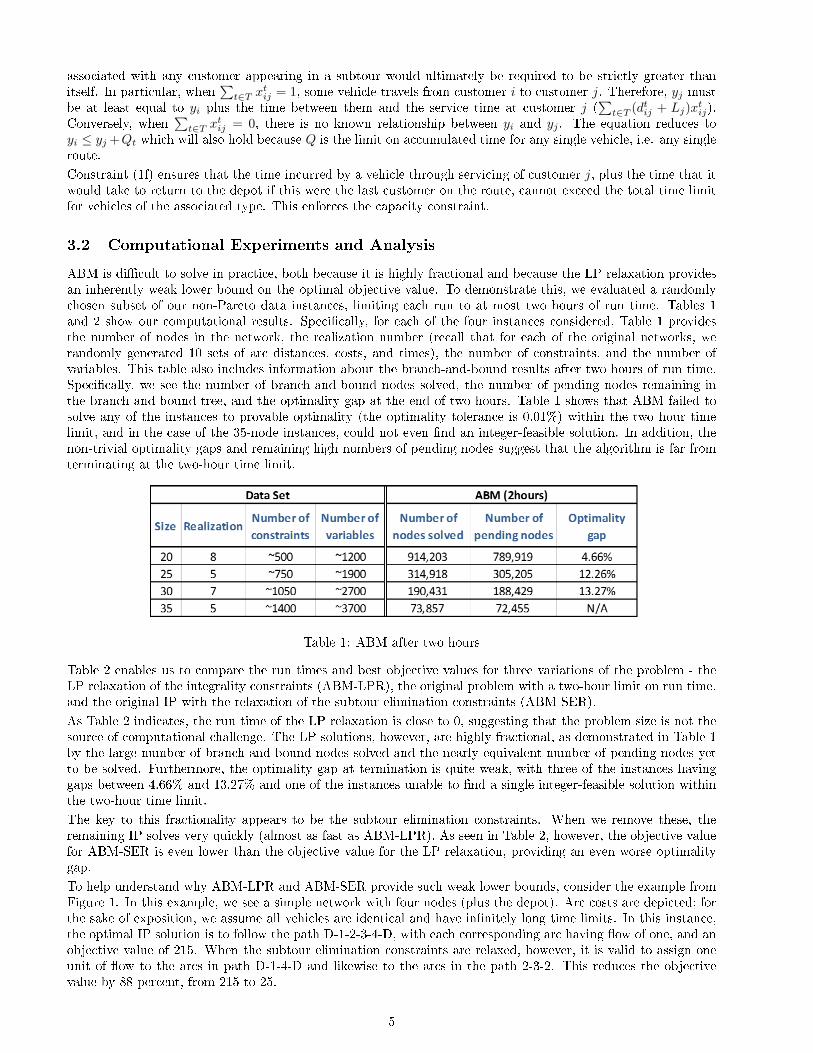
ABM is di�cult to solve in practice, both because it is highly fractional and because the LP relaxation providesan inherently weak lower bound on the optimal objective value. To demonstrate this, we evaluated a randomlychosen subset of our non-Pareto data instances, limiting each run to at most two hours of run time. Tables 1and 2 show our computational results. Speci�cally, for each of the four instances considered, Table 1 providesthe number of nodes in the network, the realization number (recall that for each of the original networks, werandomly generated 10 sets of arc distances, costs, and times), the number of constraints, and the number ofvariables. This table also includes information about the branch-and-bound results after two hours of run time.Speci�cally, we see the number of branch-and-bound nodes solved, the number of pending nodes remaining inthe branch-and-bound tree, and the optimality gap at the end of two hours. Table 1 shows that ABM failed tosolve any of the instances to provable optimality (the optimality tolerance is 0.01%) within the two hour timelimit, and in the case of the 35-node instances, could not even �nd an integer-feasible solution. In addition, thenon-trivial optimality gaps and remaining high numbers of pending nodes suggest that the algorithm is far fromterminating at the two-hour time limit.

Table 1: ABM after two hours

Table 2 enables us to compare the run times and best objective values for three variations of the problem - theLP relaxation of the integrality constraints (ABM-LPR), the original problem with a two-hour limit on run time,and the original IP with the relaxation of the subtour elimination constraints (ABM-SER).

As Table 2 indicates, the run time of the LP relaxation is close to 0, suggesting that the problem size is not thesource of computational challenge. The LP solutions, however, are highly fractional, as demonstrated in Table 1by the large number of branch-and-bound nodes solved and the nearly equivalent number of pending nodes yetto be solved. Furthermore, the optimality gap at termination is quite weak, with three of the instances havinggaps between 4.66% and 13.27% and one of the instances unable to �nd a single integer-feasible solution withinthe two-hour time limit.

The key to this fractionality appears to be the subtour elimination constraints. When we remove these, theremaining IP solves very quickly (almost as fast as ABM-LPR). As seen in Table 2, however, the objective valuefor ABM-SER is even lower than the objective value for the LP relaxation, providing an even worse optimalitygap.

To help understand why ABM-LPR and ABM-SER provide such weak lower bounds, consider the example fromFigure 1. In this example, we see a simple network with four nodes (plus the depot). Arc costs are depicted; forthe sake of exposition, we assume all vehicles are identical and have in�nitely long time limits. In this instance,the optimal IP solution is to follow the path D-1-2-3-4-D, with each corresponding arc having �ow of one, and anobjective value of 215. When the subtour elimination constraints are relaxed, however, it is valid to assign oneunit of �ow to the arcs in path D-1-4-D and likewise to the arcs in the path 2-3-2. This reduces the objectivevalue by 88 percent, from 215 to 25.

5

Table 2: Optimal cost of relaxations

Figure 1: Example of weak lower bounds

Finally, when the subtour constraints are included but the integrality requirements are relaxed, we can assign αunits of �ow to each arc in the path D-1-2-3-4-D (the solution to ABM), and 1− α units to the arcs in the pathD-1-4-D and 2-3-2 (the solution to ABM-SER), i.e. ABM-LPR is a convex combination of ABM and ABM-SER,where α approaches 0 as Q goes to in�nity.

4 Path-Based Model

Motivated by the computational experiments described in Section 3, we seek an approach that is not hampered bythe need for subtour elimination. In this section, we introduce a path-based model that, by explicitly constructingpaths as an input to the model, eliminates the need for such constraints.

Notation

Parameters and SetsN set of customers in the network, where index 0 represents the depotT set of vehicles typesRt set of all feasible routes (i.e. paths) for vehicle type t ∈ Tctr travel cost of route r for vehicle type t, ∀t ∈ T, ∀r ∈ Rtδtir binary coe�cient that takes value 1 if customer i belongs to route r for vehicle type t, else 0,

∀i ∈ N \ 0, t ∈ T, r ∈ RtMt number of available vehicles of type t, ∀t ∈ TQt time limit for vehicle type t, ∀t ∈ TLi service time at customer i, ∀i ∈ N \ 0

Variablesxtr binary variable that takes value 1 if route r is assigned to a vehicle of type t, else 0, ∀t ∈ T, ∀r ∈ RtPath-Based Model (PBM):

6

min∑t∈T

∑r∈Rt

ctrxtr (2a)

subject to:∑t∈T

∑r∈Rt

δtirxtr = 1 ∀i ∈ N \ 0 (πi) (2b)

∑r∈Rt

xtr ≤Mt ∀t ∈ T (µt) (2c)

xtr ∈ {0, 1} ∀t ∈ T, ∀r ∈ Rt (2d)

The objective (2a) minimizes the total routing cost.

Constraint set (2b) requires that each customer must be covered by exactly one route.

Constraint set (2c) speci�es that at most Mt routes are assigned to vehicles of type t ∈ T .

In addition, we associate dual variables πi and µt with (2b) and (2c), respectively.

5 Solving PBM

5.1 Column Generation Overview

PBM contains too many variables to solve explicitly except for very small problem instances. We thereforepropose to use column generation [6, 13] to solve the LP relaxation (PBM-LPR). Speci�cally, we begin with aninitial subset of the feasible columns (i.e. routes), which we call the restricted master problem (RPBM-LPR). Wethen use a pricing problem to identify promising new routes to add to RPBM-LPR, based on the dual values ofthe current optimal solution. If such columns (i.e. routes) are found, they are used to augment RPBM-LPR andthe process repeats. An optimal solution to the LP relaxation is guaranteed when no new negative reduced costroutes can be found.

Reduced Cost:

For a given feasible route rt ∈ Rt where γtijr is a binary parameter specifying whether arc (i, j) is included inroute rt, the corresponding reduced cost equation is:

RCtr = ctr −∑i∈N

πiδtir − µt

=∑i∈N

∑j∈N

ctijγtijr −

∑i∈N

πi(∑j∈N

γtijr)− µt

=∑i∈N

∑j∈N

(ctij − πi)γtijr − µt

To �nd a negative reduced cost column for vehicles of type t, or to prove that no such columns exist, we canformulate the following optimization problem:

min∑i∈N

∑j∈N

(ctij − πi)δtijr − µt (3a)

subject to: rt ∈ Rt (3b)

For the remainder of this section, we focus primarily on solving PBM-LPR and, in particular, the pricing prob-lem. When we solve the integer version of the problem, we do so heuristically. That is, for the simplicity ofimplementation, we solve the LP to optimality and then �nd the best IP solution relative to the current set ofcolumns in the restricted master. In practice, it would be necessary to generate new columns at each subsequentnodes of the branch-and-bound tree in order to ensure a provably optimal solution.

7

5.2 Dynamic Programming Approaches to Solving the Pricing Problem

The key challenge in solving PBM-LPR is in solving the pricing problem, i.e. in generating candidate routes(negative reduced cost pivot variables). In theory, this problem ((3a) and (3b)) could be formulated as a MIP.However this will result in the same di�culties observed in the arc-based formulation, such as fractionality in theLP relaxation and a weak lower bound, due to the sub-tour elimination (1e) and time limit constraints (1f), whichmust now be shifted into the pricing problem. We therefore instead take a dynamic programming (DP) approachin which, by constructing the routes dynamically, we naturally avoid sub-tours. Throughout the remainder ofthis section, we present and compare several DP algorithms for solving the pricing problem.

5.2.1 Elementary Shortest Path Problem with Resource Constraints

The pricing problem for PBM-LPR can be posed as an Elementary Shortest Path Problem with Resource Con-straints (ESPPRC). This problem identi�es minimum-cost elementary paths (i.e. paths without any embeddedcycles) that do not violate some sort of resource constraint. In our case, the resource is time (which is consumedover both arcs and nodes), and the cost is the reduced cost associated with the route when included in therestricted master. That is, we consider the true cost (which is the sum of all the arc costs) minus the dualvalue associated with each node minus the dual value associated with the speci�c vehicle type. In particular, onereduced cost problem can be solved for each vehicle type, in which the corresponding costs (true and dual) areassigned to individual arcs within the network.

Feillet et al. [15] were the �rst to propose an exact dynamic programming algorithm for solving the pricingproblem of the Vehicle Routing Problem with Time Windows (VRPTW) where paths with embedded cycles areforbidden. Other re�nements for the DP algorithm have also been suggested by Chabrier [5], and Righini andSalani [35, 36]. While DP can be a good candidate approach for solving the pricing problem for some VRPs [34],the exponential rise in the state-space can be burdensome in other cases. For example, the success of Feillet etal. [15] depends on the use of narrow time windows to facilitate pruning. On the other hand, when time windowsare too wide, the computational performance su�ers signi�cantly.

In TCHVRP, we encounter tractability issues associated with the limited opportunity to prune. Although we canuse the vehicle time limits and the fact that nodes cannot be repeated to prune, these are not su�cient. Ideally,we also want to prune whenever two partial paths meet at the same node but with di�erent costs and consumedtimes. Speci�cally, given two partial routes p1 and p2 that terminate at the same node, p1 is dominated by p2and therefore p1 can be pruned, if: 1) p1 is more costly than p2; 2) p1 takes longer than p2. We also need a thirdcriterion, however: 3) the set of nodes included in p1 is a superset of the nodes included in p2.

The third criteria is necessary to ensure equivalent remaining opportunities to capture the bene�t of negativedual values. For example, consider partial paths p1: D −X − Y − Z and p2: D −W − Z. We are tempted toprune p1 if it is higher cost and consumes more time than path p2. However, it may be the case that the optimal(i.e. most negative reduced cost) path is D −X − Y − Z −W −D. If we prune p1, we will not encounter thispath. Conversely, the path D −W − Z −W −D (which should be both cheaper and less time consuming thanD − X − Y − Z −W − D) is not actually a valid path because it repeats node W (and thus accumulates thedual value associated with the cover constraint for node W twice). Thus we can only prune p1 if it is not onlymore costly and more time consuming than p2 but also if it includes a superset of the nodes found in partial pathp2. This criteria greatly reduces the pruning opportunities, with signi�cant negative impact on computationalperformance, as we demonstrate below.

To evaluate the ESPPRC approach, considering both run time and solution quality, we conducted two experi-ments, using the data sets described in Section 2.3 and detailed in Appendix A. First, we compared the optimalobjective values of the LP relaxations of the arc-based model to the path-based model. Second, we compared theheuristic objective values found by (a) solving the LP relaxation of the path-based model to optimality and then�nding the optimal integer solution with respect to the given columns in the restricted master problem versus(b) allowing the arc-based integer model to run for the same amount of time as the path-based model and takingthe best integer feasible solution.

Consistently, we observed that the LP relaxation of the path-based model is substantially higher than that ofthe arc-based model, thus yielding a tighter lower bound. As seen in Columns ABM-LPR and ESPPRC-LPRof Table 3, the LP relaxation of the path-based model ranges from 18.33% to 32.75% higher than the arc-basedmodel, with an average increase of 25.68%.

To compare the objective values, we solved the path-based LP relaxation to optimality, then found the bestinteger solution relative to those columns. We subsequently ran the arc-based integer model for the equivalent

8

amount of time and took the lowest integer solution found during that time. In the best case, the path-basedapproach found a solution that was 69.37% lower than the ABM solution. In addition, in many cases, the arc-based approach found no integer-feasible solution (i.e. N/A), while the path-based approach always did. Finally,in all but three instances, the PBM solution was strictly better than the ABM solution, and all three of thoseinstances were instances of the homogeneous version of the problem. Results for this experiment can be seen inTable 3, Columns ESPPRC-IP and Column ABM-IP.

(∆LPR = [RSPPRC_LPR]− [ABM_LPR], ∆IP = [ABM_IP]− [ESPPRC_IP])

Table 3: Solution Quality (ESPPRC)

Although the �rst two experiments show that the path-based approach yields a tighter lower bound and betterinteger solution in equivalent time, we suggest that the approach is still too slow for practical use. For example,although the path-based approach can be solved in roughly a minute for the heterogeneous non-Pareto instancewith twenty nodes, the computational time grows exponentially for this approach as the number of nodes increases,taking about two hours to solve the instances with 35 nodes. As seen in Table 4, Columns RPBM-LPR & Pricing

9

Problem and Branch & Bound for IP Heuristics, neither the LP relaxations of the restricted master nor theultimate IP itself take long to solve; total run time depends primarily on the time required to solve the DPs ateach iteration of the column generation. We therefore consider alternative approaches to solving the DP in thefollowing sections.

Table 4: Computing Time (ESPPRC)

5.2.2 Relaxed Shortest Path Problem with Resource Constraints

The DP is hard to solve when elementary paths are required because the dominance requirements signi�cantlylimit pruning opportunities. As observed by Desrochers et al. [14], removing the no-cycles restriction can greatlyreduce run times. Furthermore, even if cycles are allowed, the equality restriction in the cover constraints willprevent such routes from being included in the optimal integer solution [5]. In fact, prior to the work of Feilletet al. [15], most existing research relaxed the no-cycle constraint in order to simplify the pricing problem. Forexample, Desrochers et al. [14] presents a pseudo-polynomial primal-dual labeling algorithm to e�ectively solvethis problem.

In this section, we consider alternative ways to solve the DP without requiring elementary paths, that is, byallowing cycles. We analyze the impact of this relaxation on both the time required to solve the pricing problemand also the strength of the LP relaxation. We refer to the variation of the pricing problem in which cycles are

10

allowed as the Relaxed Shortest Path Problem with Resource Constraints (RSPPRC). In our approach to solvingRSPPRC, we recognize that when cycles are allowed, it is no longer required that the set of nodes in partial routep1 be a superset of the nodes in partial route p2 in order for p2 to dominate p1 and thus for p1 to be pruned. Itis trivial to modify our original DP algorithm for solving ESPPRC accordingly, by simply eliminating the thirdpruning criterion.

(∆ = [RSPPRC]− [ESPPRC])

Table 5: Computing Time (RSPPRC)

We conducted computational experiments on the same data as in 5.2.1 to evaluate run time, strength of the LPrelaxation, and IP-heuristic solution quality. Figure 2 presents the resulting LP relaxation bounds and objectivevalues for the IP-heuristic approaches to RSPPRC, ASPPRC (Augmented RSPPRC de�ned later) and ESPPRC.Note that the �rst column of table 3, 4 and 5 provides a unique index for each instance and x axis in Figure2 correspond to these indices. We observe that, by simply enabling a greater degree of pruning, we can solveRSPPRC much more quickly than ESPPRC, as demonstrated in Table 5. As seen in Figure 2, however, theLP relaxation is signi�cantly worse relative to when using ESPPRC (although still signi�cantly better than theLP relaxation of the arc-based model, ABM-LPR). In turn, as seen in Figure 2, the quality of the heuristic IPsolution (found when branching just on those columns found when solving for the LP relaxation) is worse thanthe ESPPRC approach as well.

To understand why the LP relaxation when cycles are allowed is worse than ESPPRC, consider the following

11

(Percentage di�erence of ESPPRC-LPR and ABM-LPR based on SPPRC-LPR)

(Percentage di�erence of RSPPRC-IP and ESPPRC-IP based on ASPPRC-IP)

Figure 2: Solution Quality (RSPPRC)

12

example, as depicted in Figure 3. The true cost of path D − A − B − C −D is 206 and this path covers nodesA,B, and C. When cycles are allowed, however, we can replace this variable with a variable corresponding tothe path D −A−B −C −A−B −C −D, with value 1/2. Again, this covers nodes A,B, and C, but now withcost 106. The reduction is because we have reduced the travel distance from the depot to the cluster of nodes.Extending this idea, consider traversing the cycle A − B − C − A m times with corresponding value x = 1

m .Again, in the LP relaxation, this would satisfy coverage of A,B, and C, but with a cost of 6m

m+1 + 206m+1 . As m

approaches in�nity, the cost approaches six, the cost of the cycle A− B − C − A. The only limiting factor hereis the total time limit Q allowed for the path.

Figure 3: Weak lower bound by the no-cycle constraint relaxation

In addition, the IP heuristic objective is also worse because many of the columns identi�ed when solving PBM-LPR using RSPPRC will not in fact be valid columns for the integer version of the problem because, as motivatedin the previous example, many will contain cycles which are invalid under the equality constraints. Since we arenot generating columns beyond the root node, this is particularly problematic.

Motivated by this, we augmented the RSPPRC approach to include the acyclic equivalent of each newly-generatedcolumn. That is, given a column where some node occurs more than once, we also create a new column in whichwe delete from the route all occurrences of that node except the �rst. We refer to this augmented RSPPRCas ASPPRC. Note that this does not impact the LP relaxation of RSPPRC (because these were not chosen tobe included in the optimal LP solution), nor does it have any signi�cant impact on the run time over solvingRSPPRC. Therefore, ASPPRC is equivalent in run time to RSPPRC. For solution quality, as seen in Figure 2,ASPPRC is always better than RSPPRC (given that it has a superset of the columns of RSPPRC), however, itstill has worse objective values than ESPPRC.

5.2.3 ESPPRC with Weak Dominance Rule

In the previous sections, we observed that allowing cycles made the DP approach much faster because we were notlimited to pruning only when one path contained a superset of the nodes in another. On the other hand, allowingcycles greatly weakened the lower bound. Motivated by these facts, we propose a �nal alternative approach inwhich we do not allow cycles, but we eliminate the third pruning criterion. For example, if path p1 is less costlyand takes less time than path p2, we allow path p2 to be pruned, even if it does not contain a superset of the nodesin path p1. We refer to this ESPPRC with weak dominance rule as WESPPRC. Note that this new approach nolonger guarantees an optimal solution to the LP relaxation because we may prune a path that is in fact part ofthe optimal solution.

We observe, as seen in Table 6, that the result is a signi�cant improvement in run time - in one instance, frommore than three hours to roughly 34 seconds. We reiterate that the LP relaxation of WESPPRC is not guaranteedto be optimal (i.e. we may prune relevant columns). As seen in Table 6, however, the impact on the LP relaxationis very small, with a maximum increase of 0.94%. Finally, we note that the IP objective value of WESPPRC issometimes worse and sometimes better than ESPPRC. However, we observe the di�erence in objective value to

13

be within 5.24% in all cases, and often much less. Furthermore, it is as good or better than ASPPRC in all butone of the large problem instances, and faster than that approach in most cases.

Table 6: Computing Time & Solution Quality (WESPPRC)

6 Conclusions

In this paper, we present a variation of VRP, TCHVRP, in which arc times and costs vary by vehicle type,and in particular, Pareto dominance is not assumed. We demonstrate the challenges of solving this problemwith an arc-based model and consider a path-based model as a viable alternative. In particular, we focus ondynamic programming-based approaches to solving the pricing problem when solving the path-based formulationvia column generation. We show that allowing cycles within the routes makes DP approaches to generating routesmuch faster, but at the expense of a weaker LP relaxation and poorer integer solutions when routes are generatedonly at the root node. We also show that prohibiting cycles, with fully-de�ned pruning, is prohibitive slow. Asan alternative, we propose a heuristic where cycles are not allowed, but pruning is expanded to allow those caseswhere set of the nodes covered by one partial route is not necessarily a superset of the nodes covered by another.Although we can no longer guarantee the optimality of the LP relaxation, we show that this markedly improvessolution time over the pure case and markedly improves solution quality over the case in which cycles are allowed.

14

A Problem Data

We generate TCHVRP instances based on the data sets of Golden et al. [25], which is popular benchmarktest instances commonly used in the literature. Table 7 gives the characteristics of the TCHVRP instances wehave generated. In this table, we give the number N of customers and, for each vehicle type k, the numberMk of vehicles available, the variable cost factor αk and time factor βk, error terms for cost εα and time εβ ,and the number of instances. As global parameter settings, we use the constant capacity Q and loading time Lover all vehicles. Finally, we generate three di�erent data sets for TCHVRP: single �eet type with Pareto cost,heterogeneous �eet with Pareto cost, and heterogeneous �eet with non-Pareto cost.

For Pareto instances, we have a �xed cost per mile and distance per hour for each vehicle type. For Non-Paretoinstances, we generate the cost per mile (αij) and distance per hour (βij) from a normal distribution with themeans and standard deviations in Table 7. More precisely, the travel cost ckij and time tkij between customers i

and j for vehicles of type k are calculated by ckij = αkijdij and tkij =

dijβkij

when the travel is performed by a vehicle

of type k. These are based o� of a Euclidean distance matrix Dij from the geographical data given in Golden etal. [25]. And then, we generate cost and time matrix such that cost = αij ×Dij and time = Dij

βijgiven distance

matrix Dij .

For the time resources constraints, we have chosen to use a single value Q = 8 hours for all vehicles, and a loadingtime of L = 30 minutes for all customer nodes for all vehicle types. Our choice of Q and L is motivated by thefact that we wanted vehicle tours of approximately 9 to 12 nodes per route.

Finally, the error terms αk and βk have been chosen in such a way that no vehicle speed is less than 30 mph ormore than 60 mph and cost is between 1.25 and 3.75 dollars per mile.

Table 7: Parameters for instances

15

References

[1] Yogesh Agarwal, Kamlesh Mathur, and Harvey M Salkin. A set-partitioning-based exact algorithm for thevehicle routing problem. Networks, 19(7):731�749, 1989.

[2] Roberto Baldacci, Maria Battarra, and Daniele Vigo. Routing a heterogeneous �eet of vehicles. In Thevehicle routing problem: latest advances and new challenges, pages 3�27. Springer, 2008.

[3] Roberto Baldacci, Nicos Christo�des, and Aristide Mingozzi. An exact algorithm for the vehicle rout-ing problem based on the set partitioning formulation with additional cuts. Mathematical Programming,115(2):351�385, 2008.

[4] Michel L Balinski and Richard E Quandt. On an integer program for a delivery problem. OperationsResearch, 12(2):300�304, 1964.

[5] Alain Chabrier. Vehicle routing problem with elementary shortest path based column generation. Computers& Operations Research, 33(10):2972�2990, 2006.

[6] Eunjeong Choi and Dong-Wan Tcha. A column generation approach to the heterogeneous �eet vehiclerouting problem. Computers & Operations Research, 34(7):2080�2095, 2007.

[7] Nicos Christo�des. The vehicle routing problem. RAIRO-Operations Research-Recherche Opérationnelle,10(V1):55�70, 1976.

[8] Nicos Christo�des, Aristide Mingozzi, and Paolo Toth. Exact algorithms for the vehicle routing problem,based on spanning tree and shortest path relaxations. Mathematical programming, 20(1):255�282, 1981.

[9] Nicos Christo�des, Aristide Mingozzi, and Paolo Toth. State-space relaxation procedures for the computationof bounds to routing problems. Networks, 11(2):145�164, 1981.

[10] G u Clarke and JW Wright. Scheduling of vehicles from a central depot to a number of delivery points.Operations research, 12(4):568�581, 1964.

[11] G Dantzig, R Fulkerson, and S Johnson. Solution of a large-scale traveling-salesman problem. OperationsResearch, 2(4):393�410, 1954.

[12] George B Dantzig and John H Ramser. The truck dispatching problem. Management science, 6(1):80�91,1959.

[13] George B Dantzig and Philip Wolfe. Decomposition principle for linear programs. Operations research,8(1):101�111, 1960.

[14] Martin Desrochers, Jacques Desrosiers, and Marius Solomon. A new optimization algorithm for the vehiclerouting problem with time windows. Operations research, 40(2):342�354, 1992.

[15] Dominique Feillet, Pierre Dejax, Michel Gendreau, and Cyrille Gueguen. An exact algorithm for the el-ementary shortest path problem with resource constraints: Application to some vehicle routing problems.Networks, 44(3):216�229, 2004.

[16] Brian A Foster and David M Ryan. An integer programming approach to the vehicle scheduling problem.Operational Research Quarterly, pages 367�384, 1976.

[17] Ricardo Fukasawa, Humberto Longo, Jens Lysgaard, Marcus Poggi de Aragão, Marcelo Reis, Eduardo Uchoa,and Renato F Werneck. Robust branch-and-cut-and-price for the capacitated vehicle routing problem.Mathematical programming, 106(3):491�511, 2006.

[18] WW Garvin, HW Crandall, JB John, and RA Spellman. Applications of linear programming in the oilindustry. Management Science, 3(4):407�430, 1957.

[19] Bezalel Gavish and Stephen C Graves. The travelling salesman problem and related problems. 1978.

[20] Bezalel Gavish and Stephen C Graves. Scheduling and routing in transportation and distribution systems:formulations and new relaxations. Management Science (accepted. subject to revision), 1982.

16

[21] Michel Gendreau, Gilbert Laporte, Christophe Musaraganyi, and Éric D Taillard. A tabu search heuristicfor the heterogeneous �eet vehicle routing problem. Computers & Operations Research, 26(12):1153�1173,1999.

[22] Filip Gheysens, Bruce Golden, and Arjang Assad. A comparison of techniques for solving the �eet size andmix vehicle routing problem. Operations-Research-Spektrum, 6(4):207�216, 1984.

[23] Billy E Gillett and Leland R Miller. A heuristic algorithm for the vehicle-dispatch problem. Operationsresearch, 22(2):340�349, 1974.

[24] Fred Glover. Tabu search-part i. ORSA Journal on computing, 1(3):190�206, 1989.

[25] Bruce Golden, Arjang Assad, Larry Levy, and Filip Gheysens. The �eet size and mix vehicle routing problem.Computers & Operations Research, 11(1):49�66, 1984.

[26] Bruce L Golden, Subramanian Raghavan, and Edward A Wasil. The Vehicle Routing Problem: LatestAdvances and New Challenges: latest advances and new challenges, volume 43. Springer, 2008.

[27] John H Holland. Adaptation in natural and arti�cial systems: An introductory analysis with applications tobiology, control, and arti�cial intelligence. U Michigan Press, 1975.

[28] Scott Kirkpatrick, MP Vecchi, et al. Optimization by simmulated annealing. science, 220(4598):671�680,1983.

[29] Gilbert Laporte. Fifty years of vehicle routing. Transportation Science, 43(4):408�416, 2009.

[30] Clair E Miller, Albert W Tucker, and Richard A Zemlin. Integer programming formulation of travelingsalesman problems. Journal of the ACM (JACM), 7(4):326�329, 1960.

[31] Yuichi Nagata. Edge assembly crossover for the capacitated vehicle routing problem. In EvolutionaryComputation in Combinatorial Optimization, pages 142�153. Springer, 2007.

[32] Christian Prins. A grasp × evolutionary local search hybrid for the vehicle routing problem. In Bio-inspiredalgorithms for the vehicle routing problem, pages 35�53. Springer, 2009.

[33] MR Rao and S Zionts. Allocation of transportation units to alternative trips-a column generation schemewith out-of-kilter subproblems. Operations Research, 16(1):52�63, 1968.

[34] Giovanni Righini and Matteo Salani. Dynamic programming algorithms for the elementary shortest pathproblem with resource constraints. Electronic Notes in Discrete Mathematics, 17:247�249, 2004.

[35] Giovanni Righini and Matteo Salani. Symmetry helps: bounded bi-directional dynamic programming forthe elementary shortest path problem with resource constraints. Discrete Optimization, 3(3):255�273, 2006.

[36] Giovanni Righini and Matteo Salani. New dynamic programming algorithms for the resource constrainedelementary shortest path problem. Networks, 51(3):155�170, 2008.

[37] Éric D Taillard and Québec) Centre for Research on Transportation (Montréal. A heuristic column generationmethod for the heterogeneous �eet vrp. Operations Research, 33(1):1�14, 1999.

[38] Paolo Toth and Daniele Vigo. The vehicle routing problem. Siam, 2001.

17