A TIME BOMB FOR THE EURO? Understanding Germany's … · imports and exports continues, ... 1.1...
97
STUDY No. 59 • March 2018 • Hans-Böckler-Stiftung A TIME BOMB FOR THE EURO? UNDERSTANDING GERMANY’S CURRENT ACCOUNT SURPLUS Jan Priewe 1 Abstract The paper analyses the rise of the current account balance in Germany by around ten percentage points (relative to GDP) in the period 1999-2016. A big part of the rise is due to subdued domestic final demand which tends to suppress growth of imports. This demand-side effect has to do with weak wage dynamics, unequal income distribution and fiscal restraint. Despite ups and downs, the trend seems to be persistent. On the supply side, the cost and price competitiveness of the German economy is superior in European comparison. However, much more important is the superior non- price competitiveness in various dimensions. Exports grow in line with world exports which tend to grow markedly faster than imports and GDP in Germany. If this wedge between growth rates of imports and exports continues, the current account tends to rise, irrespective of short-term ups and downs. Germany follows an unsustainable trend. On the supply side, it is the strength of German manufacturing, the basis of the country’s surplus. It has emerged in parallel with a process of creeping deindustrialisation in other EMU member states. The export championship, seemingly the crown jewel of the economy, has the mirror image of an Achilles heel. The surplus cannot be understood without the dysfunctions of the EMU which has no mechanisms to prevent and correct current account imbalances. Many policy makers are blinded by export success and vested interests of German export indus- tries. They trust in “laisser-faire” and “no activism” advice, in contrast to concerns from the Europe- an Commission and the IMF. In this sense, there exists a time-bomb for the cohesion of the Euro area. 1 Prof. (em.) from HTW Berlin – University of Applied Sciences, Senior Research Fellow at Economic Policy Institute (IMK) in Hans-Böckler-Foundation, Düsseldorf, Contact address [email protected]. —————————
Transcript of A TIME BOMB FOR THE EURO? Understanding Germany's … · imports and exports continues, ... 1.1...
STUDY
No. 59 • March 2018 • Hans-Böckler-Stiftung
A TIME BOMB FOR THE EURO? UNDERSTANDING GERMANY’S CURRENT ACCOUNT SURPLUS
Jan Priewe1
Abstract
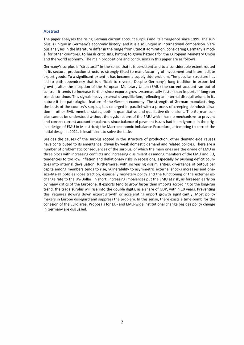
The paper analyses the rise of the current account balance in Germany by around ten percentage points (relative to GDP) in the period 1999-2016. A big part of the rise is due to subdued domestic final demand which tends to suppress growth of imports. This demand-side effect has to do with weak wage dynamics, unequal income distribution and fiscal restraint. Despite ups and downs, the trend seems to be persistent. On the supply side, the cost and price competitiveness of the German economy is superior in European comparison. However, much more important is the superior non-price competitiveness in various dimensions. Exports grow in line with world exports which tend to grow markedly faster than imports and GDP in Germany. If this wedge between growth rates of imports and exports continues, the current account tends to rise, irrespective of short-term ups and downs. Germany follows an unsustainable trend.
On the supply side, it is the strength of German manufacturing, the basis of the country’s surplus. It has emerged in parallel with a process of creeping deindustrialisation in other EMU member states. The export championship, seemingly the crown jewel of the economy, has the mirror image of an Achilles heel. The surplus cannot be understood without the dysfunctions of the EMU which has no mechanisms to prevent and correct current account imbalances.
Many policy makers are blinded by export success and vested interests of German export indus-tries. They trust in “laisser-faire” and “no activism” advice, in contrast to concerns from the Europe-an Commission and the IMF. In this sense, there exists a time-bomb for the cohesion of the Euro area.
1 Prof. (em.) from HTW Berlin – University of Applied Sciences, Senior Research Fellow at Economic Policy Institute (IMK) in Hans-Böckler-Foundation, Düsseldorf, Contact address [email protected].
—————————
A Time Bomb for the Euro? Understanding Germany’s Current Account Surplus
Jan Priewe
Prof. (em.) from HTW Berlin – University of Applied Sciences Senior Research Fellow at Economic Policy Institute (IMK) in Hans Böckler Foundation, Düsseldorf
Outline
0. Introduction 1. Germany’s rising surplus – overview on key empirical features
1.1 Basic overview 1.2 Supply-side structure, macroeconomic performance and financial issues
2. Understanding current account surpluses 2.1 The view on the determinants of trade 2.2 The view on the determinants of saving and investment 2.3 Combining the trade and saving view 2.4 Constraints for surpluses and deficits
3. The emergence of the German surplus – empirical findings 3.1 The wedge in growth of exports and imports 3.2 Can exchange rates rebalance current accounts? 3.3 Excess saving – weak domestic demand 3.3.1 Does “aging” explain the strong current account – and prospective rebalancing? 3.3.2 Saving rose, investment fell, current account up 1999-2016 3.4 Is there a lack of competitiveness in the deficit countries? 3.5 Summing up – Germany’s “super competitiveness”
4. Alarming trade balance projection 2016-2026 5. “International competitiveness” – a dangerous obsession 6. Why is the German surplus a problem? 7. When is a current account surplus “excessive” – and what should be done?
8. Conclusions and policy options 8.1 “Activism is Inappropriate” regarding surpluses within EMU?
8.2 Policy options in Germany 8.3 Reforms at the EU level
9. Outlook References Appendix
1
Abstract
The paper analyses the rising German current account surplus and its emergence since 1999. The sur-plus is unique in Germany’s economic history, and it is also unique in international comparison. Vari-ous analyses in the literature differ in the range from utmost admiration, considering Germany a mod-el for other countries, to harsh criticisms, hinting to grave hazards for the European Monetary Union and the world economy. The main propositions and conclusions in this paper are as follows.
Germany’s surplus is “structural” in the sense that it is persistent and to a considerable extent rooted in its sectoral production structure, strongly tilted to manufacturing of investment and intermediate export goods. To a significant extent it has become a supply side-problem. The peculiar structure has led to path-dependency that is difficult to reverse. Despite Germany’s long tradition in export-led growth, after the inception of the European Monetary Union (EMU) the current account ran out of control. It tends to increase further since exports grow systematically faster than imports if long-run trends continue. This signals heavy external disequilibrium, reflecting an internal disequilibrium. In its nature it is a pathological feature of the German economy. The strength of German manufacturing, the basis of the country’s surplus, has emerged in parallel with a process of creeping deindustrialisa-tion in other EMU member states, both in quantitative and qualitative dimensions. The German sur-plus cannot be understood without the dysfunctions of the EMU which has no mechanisms to prevent and correct current account imbalances since balance of payment issues had been ignored in the orig-inal design of EMU in Maastricht; the Macroeconomic Imbalance Procedure, attempting to correct the initial design in 2011, is insufficient to solve the tasks.
Besides the causes of the surplus rooted in the structure of production, other demand-side causes have contributed to its emergence, driven by weak domestic demand and related policies. There are a number of problematic consequences of the surplus, of which the main ones are the divide of EMU in three blocs with increasing conflicts and increasing dissimilarities among members of the EMU and EU, tendencies to too low inflation and deflationary risks in recessions, especially by pushing deficit coun-tries into internal devaluation; furthermore, with increasing dissimilarities, divergence of output per capita among members tends to rise, vulnerability to asymmetric external shocks increases and one-size-fits-all policies loose traction, especially monetary policy and the functioning of the external ex-change rate to the US-Dollar. In short, increasing imbalances put the EMU at risk, as foreseen early on by many critics of the Eurozone. If exports tend to grow faster than imports according to the long-run trend, the trade surplus will rise into the double digits, as a share of GDP, within 10 years. Preventing this, requires slowing down export growth or accelerating import growth significantly. Most policy makers in Europe disregard and suppress the problem. In this sense, there exists a time-bomb for the cohesion of the Euro area. Proposals for EU- and EMU-wide institutional change besides policy change in Germany are discussed.
2
Abbreviations BoP Balance of Payments BoPCG BoP constrained growth CAB Current account balance CAS Current account surplus CEE German Council if Economic Experts DE Germany EC European Commission ECB European Central Bank EMU European Monetary Union EU European Union GCF Gross capital formation GDP Gross domestic product GFCF Gross fixed capital formation GIIPS Greece, Ireland, Italy, Portugal, Spain GNI Gross National Income GRH Golden rule hypothesis IC International competitiveness IMF International Monetary Fund M imports MIP Macroeconomic Imbalance Procedure MLC Marshall-Lerner condition
NIIP Net international investment position NX net exports OECD Organisation for International Co-operation and Development ppts percentage points PtM Pricing to markets REER Real effective exchange rate RERHH Real exchange rate hypotehsis Rhs right hand scale RoW Rest of the world TARGET2 Trans-European Automated Re-al-time Gross Settlement Express Transfer System TB Trade balance UK United Kingdom ULC Unit labour costs VA value added VAT value added tax WDI World development indicators X exports yoy year over year
List of graphs, tables and boxes Graphs 1.1 Germany: Current account balance and its components, % of GDP 1.2 Current account balances of members of the Euro Area 1.3 Germany’s trade balance (goods) with EMU, other EU and extra EU countries (German data) 1.3a Germany’s Intra EU net exports (Destatis and AMECO data) 1.4 Germany: Growth of exports and imports (including services), GDP, domestic demand, GDP defla-tor 1.5 Export shares in world exports (goods and services, measured in current Euro) 1.6 Market shares: exports of goods and services to total exports, 1999-2016, change in ppts 1.7 Germany: exports and imports of goods and services, % of GDP 1.8 Manufacturing value added, % of GDP, in selected countries 1.9 Manufacturing in Germany 1999-2016, as % of GDP 1.10 GDP growth 1999-16 in constant prices, % p.a., in EU and selected other OECD countries 1.11 Index of the price deflator for exports and services – selected EMU countries, 1999 = 100 1.12 Net international investment position in 28 EU member states, 2016, Quarter 4, % of GDP 1.13 Net international investment position of EMU countries, bn Euro 1.14 Net international investment position, % of GDP, in selected EMU countries 1999-2016 3.1 Growth of Germany’s exports and imports, world GDP and world exports (in current Euro) 3.2 Germany: Growth of exports and imports and annual change of net exports, % of GDP 3.3 Exports’ minus imports’ growth rate in selected countries 3.4 Germany: Unit labour costs and price indices 3.5 Real effective exchange rates against 67 countries, CPI based, 1999-2016 3.6 Switzerland: current account balance and real effective exchange rate 3.7 Germany: Saving rate of private households, % of disposable income 3.8 Germany: 1999-2016: demographic change 3.9 Germany: aging society 2015-30 3.10 Dependency ratios in major EMU countries 3.11 Sectoral savings and current account balance, bn Euro 3.12 Increase 1999-2016 of sectoral savings, investment and current account balance, % of GDP 3.13 Germany: contribution of nominal growth of domestic demand and net exports 3.14 Trade balance (goods and services) in selected EMU countries
3

3.15 EMU members: contribution of net exports to GDP-increase 2009-2016 Graphs in the appendix A1 Current account balance in selected countries, % of GDP, 1980-2016 A2 Trade balance (goods and services) and current account balance, % of GDP, in West Germany and re-united Germany 1960-2016 A3 Germany: trade balance (without services), composition with types of goods, bn Euro A4 Germany: Germany’s trade surplus: sectoral composition, % of GDP A5 Germany’s trade balance (without services) 2002-2016 in bn Euro by region of trade partners A6 Germanys trade balance (goods): change in bilateral balances in bn Euro 2002-2016 by region A7 Saving rates of private households, % of disposable income, selected countries A8 German exports of goods and services in current and constant prices, terms of trade A9 Germany’s price competitiveness, measured by real effective exchange rates and unit labour costs A10 Adjusted wage share in major EMU countries A11 Germany: shrinking fixed capital formation, % of GDP A12 Current account balance, as budget balance plus private sector balance, % of GDP (for Germany, Greece, Ireland, Spain) A13 Current account balance in China and Germany, 1999-2016, % of GDP Tables 1.1 Surplus and deficit countries in EU/EMU 1.2 Import content of exports and other indicators 1.3 Manufacturing value added in EMU countries 1999-2016 (2010 prices) 1.4 Structure of exports in selected EMU-countries 1999-2016 1.5 MIP scoreboard for Germany 2017 3.1 Reference nominal growth rates for Germany’s exports and imports 3.2 Growth of nominal exports and imports, GDP, and the trade balance in Germany 1991-2016 3.3 Germany 1999-2016: contributions to GDP growth 3.4 Ex- and imports in crisis countries of EMU 4.1 Six projections for the trade balance 2026 and 20121 Boxes Box 6.1: Germany’s burden with its high surplus Box 6.2 The burden of deficit countries in the EMU
4
0. Introduction
Current account imbalances are one of the key problems of the European Monetary Union (EMU) and the entire EU. The EMU tends to be divided in a surplus bloc headed by Germany and a deficit bloc which has improved their current account balances (CAB) recently to more or less zero or even to mild surplus. Many of these countries are likely to fall back to deficits if domestic demand im-proves. A third group of countries managed to keep their currents more or less in balance. The entire EMU faces an unprecedented surplus, driven by the surplus bloc. The spread between top and low balances of members, as a share of GDP, is for many above eight percentage points (ppts), ranging from -5.6% (Cyprus) to France (-0.9%) to Germany with 8.3%, and the median at 1.8% (AMECO, for 2016). Germany entered the EMU 1999 with a deficit of -1.7%, and moved by 10 ppts to its peak of 8.3% in 2016. It was not a continuous move, but a clear trend upward, unprecedented in Germany’s history (see graph A9 in the appendix) and unique in international comparison. China pushed its sur-plus from 1.9% to 10.3% in the short period 2000-2005 but it dropped in 2016 to the old level of 2000, a full turnaround (see graph A13). Germany has by far the biggest current account surplus on the globe. Its impact is not limited to EMU or EU.
There is only a limited amount of literature on Germany’s current account surplus, despite heavy international policy debates, mirrored in the media, and despite strongly deviating analyses and con-clusions in the academic and policy related literature. There is no mainstream consensus in this issue, or put differently: there is no mainstream. The profession has no consensus. The main poles of the debates are set, firstly, by the German Council of Economic Experts (majority) (CEE 2014), secondly, by the International Monetary Fund in its 6th External Sector Report 2017 and its Article IV Review of Germany (IMF 2017a and b), and thirdly by the Country Review of Germany of the European Com-mission (EC 2017) in the framework of the Macroeconomic Imbalance Procedure (MIP). The CEE (2014) sees no problem with the German surplus, beside problems of deficits in the peripheral EMU members which did not follow sufficiently EU rules, especially regarding fiscal deficit and debt pre-scriptions. They warn against “activism” in this regard and discern no problems for Germany or the functioning of the EMU. The MIP of the EC is valued as unnecessary, since the EU’s Fiscal Compact and the Banking Union suffice to avert possible problems of imbalances.
In contrast, the IMF (2017a) identifies Germany as the biggest surplus country on the globe, heading a small group of advanced surplus countries like Japan, Korea, Switzerland, Netherlands and joined by China. The diagnosis is that this group has persistent high surpluses with severe negative reper-cussions for the global economy, which require multilateral action. The main problem of the global imbalances is seen in deflationary risks of the world economy, apart from the problems suffering from too high deficits with limited space for rebalancing. The surplus group of advanced countries has replaced since 2008 the oil exporters as the main surplus generators. Germany is advised to boost domestic demand to reduce the excessive surplus which is estimated in the range of 3-6% of GDP. The report of EC (2017) uses the guidelines and the 14 indicators of the MIP methodology and concludes that Germany’s surplus is unsustainable. The alarm lines of a 6% surplus are exceeded since 2012, the 3-years average alarm line since 2014. Despite harsh critique of the surplus, including hinting to negative spillovers for the EMU as a whole, EC does not classify Germany’s surplus as “ex-cessive”, but this conclusion does not seem to be in line with the content of the report. Classifying it as excessive would initiate a formal procedure with possible sanctions. Until now, the EC has never qualified a surplus as excessive despite a number of in-depth-reports.
The spectrum of opinions expressed in the academic literature is amazingly broad. Dustmann et al. (2015) praise Germany’s high competitiveness and award the economy the label “superstar”. Fel-bermayr, Fuest and Wollmershäuser (2017), leading economists from the German ifo-institute, see no problem in the surplus which they consider mainly rooted in demographic reasons which will lead in the future to a moderation. Similar positions are asserted by the German Federal Ministry of Fi-nance and the Federal Ministry of Economics; they hint to specific adverse shocks. Several other au-thors emphasize also a number of adverse shocks that had pushed Germany into the surplus, and
5
expect moderation in the future; they don’t analyse long-run trends. Some authors using a Dynamic Stochastic General Equilibrium Model (DSGE) hint to around two dozen different shocks which are forecast to fade away towards a moderated equilibrium surplus (Kollmann et al. 2014). It is amazing that that there are apparently so many unidirectional shocks, but no re-balancing shocks. The built-in methodology of DSGE models forecasts by rebalancing – by assumptions. The German Bundesbank (2013) argues that Germany as a mature economy tends to more saving and providing excess capital to less advanced countries and doubts that demographic change has had or will have relevant impact on the current account. Bechetoille et al. (2017) found three main contributions to the build-up of the German surplus: 3 ppts as a result of wage restraint, 2-3 ppts due to demographic factors, and the rest caused by fiscal restraint and other factors. The methodology, however, disregards demurs raised by other authors such as Horn et al. (2017) regarding the low price elasticity of trade and pric-ing to markets. Flassbeck/Lapavitsas (2013, 2015) see below average unit labour costs, austerity policies – imposed on Mediterranean EMU countries – and low growth in Germany as key causes of the surplus which is considered critical for the survival of the EMU. Gabrisch (2017) and Gabrisch/Staehr (2015) see capital flows at the root of the problem when capital exports change interest rates and real exchange rates which induce excessive net imports and as a mirror image net exports of surplus countries. Scharpf (2017 and 2017a) diagnoses a long tradition of institutional dissimilarities in the heterogeneous EMU, reflected in diverse movements of wages, prices, debt and trade, in Northern and Southern Europe which render the common currency system as unsustaina-ble. He pleas, similar to Stiglitz (2016) in one of several options proposed, for a divide of the Euro-zone in two parts, among other reasons because of the imbalances. Von Weizsäcker (2017) regards the imbalances as hazardous and sees their roots in a global “saving glut”, understood as a long-run trend to excess saving accumulated to stocks of unproductive financial wealth. In Herr/Priewe/Watt (2017), also in Sawyer (2017), the architecture of the Euro area is criticised for disregarding BoP im-balances within the EMU and not providing any policies to mitigate them, so that no replacement for nominal exchange rate adjustments exists.
When addressing the current account imbalances, first and foremost we have to understand their genesis, in particular Germany’s surplus. Therefore, we concentrate in this paper on five issues:
(1) We analyse the driving forces for the rise of the German surplus and investigate whether it is a “structural”, or an “accidental” surplus, resulting from a series of adverse shocks with a tendency to moderate in the near future. In this context we want to solve the puzzle why the dynamics of imports are so much weaker than the one for exports. We attempt to focus on the long haul 1999-2016, not an annual ups and downs.
(2) We elaborate a simple projection of the German surplus for the period 2016-2026 and look at potential market-driven stabilisers for rebalancing.
(3) We investigate whether the making of the surplus and concurrently the deficits in the South-Western periphery (and the second periphery in Eastern Europe) were caused by price or non-price competitiveness and which role real effective exchange rates as well as unit-labour (ULC) played, subject of heated debates.
(4) We discuss whether and in what ways the German surplus is problematic, both for Germany and for the functioning of the EMU. This is, amazingly, one of the key contested issues in academic dis-courses.
(5) We discuss the contours of possible policy options for Germany and the EMU in general in the framework of the MIP.
Our main propositions and conclusions are as follows. Germany’s surplus is “structural” in the sense that it is persistent and rooted in its sectoral production structure, strongly tilted to manufacturing of investment and intermediate export goods. This structure has led to path dependency that is difficult to reverse. Despite Germany’s long tradition in export-led growth, since the inception of EMU the current account ran out of control. It tends to increase further since exports grow systematically
6

faster than imports if long-run trends continue. This signals heavy external disequilibrium, reflecting an internal disequilibrium. In its nature it is a pathological feature of the German economy. The sur-plus cannot be understood without the dysfunctions of the EMU which has no satisfactory mecha-nisms to prevent and correct current account imbalances since balance of payment (BoP) issues had been ignored in the original design of EMU in Maastricht; the Macroeconomic Imbalance Procedure, attempting to correct the initial design in 2011, is insufficient to solve the tasks.
Besides the causes of the surplus in the structure of production, other causes have contributed to the surplus, mainly driven by weak domestic demand and related policies. The bulk of excessive saving emerged from the corporate sector. There are several problematic consequences of the surplus, of which the main ones are the divide of EMU in three blocs with increasing conflicts and increasing dissimilarities in EMU and EU, tendencies to too low inflation and deflationary risks in recessions, especially by pushing deficit countries into internal devaluation. Furthermore, with increasing dis-similarities, divergence of output per capita among members tends to rise, vulnerability to asymmet-ric external shocks increases and one-size-fits-all policies loose traction, especially monetary policy and the functioning of the external exchange rate to the US-Dollar. In short, increasing imbalances put the EMU at risk, as foreseen early on by many critics of the Eurozone.
We proceed as follows. In chapter 1, we provide a descriptive empirical overview on Germany’s sur-plus and its genesis, against the backdrop of the key structural features of the German economy. Chapter 2 looks at different analytical approaches regarding BoP imbalances. We discuss the deter-minants of exports and imports and the identities of national accounting, before synthesizing both views on the BoP. Chapter 3 provides more in-depth evidence on the determinants of exports and imports in the context of Germany’s often admired super-competitiveness. Based on the analysis, we calculate a simple projection of the trade surplus performance of Germany for the period 2016-26 in chapter 4. In this vein we discuss in chapter 5 the meaning of “national competitiveness” or “compet-itiveness of nations”, criticised by Krugman as “dangerous obsession”. Chapter 6 investigates the contested question what the real problems with the German surplus are. Chapter 7 discusses policy options for Germany and the reform of the MIP.
1. Germany’s rising surplus – overview on key empirical features First, we give a basic overview on the current account performance of the German economy in the period 1999-2016. Then we turn to the supply side base of German exports and the related financial issues. 1.1 Basic overview In 2016 Germany’s current account surplus (CAS) is the highest on the globe in absolute numbers, viz. 8.3% of GDP (measured in Euro). Germany is the 4th biggest economy in the world (counting the GDP in current prices). In absolute value of the surplus, number 2 and 3 are China and Japan, both around one third less than Germany’s. The German surplus is roughly 20% of all surpluses held globally, and therefore also of 20% of all deficits. The next biggest surplus makers are Korea, Switzerland, Nether-lands and Taiwan whose combined surplus is only a bit larger than Germany’s (data from WDI 2017). This demonstrates the IMF’s concern that since 2008 a group of advanced countries, besides China, is the driver of the reconfiguration of global imbalances, while OPEC countries lost their role as prime surplus countries. The spearhead of this group is Germany. The IMF (2017a) considers this surplus club as stable, without market-driven forces towards rebalancing.
The German surplus emerged from a small deficit of -1.7% 1999, the birth of the EMU, to balance in 2001, reached then 6.8% (2008) before the financial crisis during which it dropped somewhat and reached then its record peak, so far, in 2016 (graph 1.1). Hence there are four phases, the short peri-od 1999-2001, the rise by 6.8 ppts 2002-2008, after the subsequent fall in 2009 by 1.2 ppts came another rise by 2.9 ppts 2010-2016. While most of the surplus 2002-2008 occurred against other EMU and EU members which fell in strong deficits, the rise after 2009 came about with a switch to-ward surplus with extra EMU countries, especially the US, apart from the UK after the demise of the Pound Sterling (graph 1.2), hence despite appreciation of the Euro against the Pound.
7
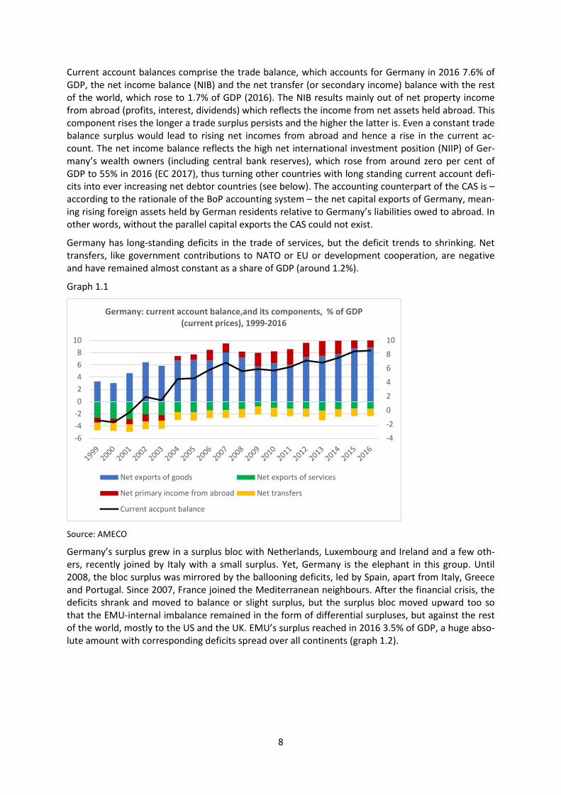
Current account balances comprise the trade balance, which accounts for Germany in 2016 7.6% of GDP, the net income balance (NIB) and the net transfer (or secondary income) balance with the rest of the world, which rose to 1.7% of GDP (2016). The NIB results mainly out of net property income from abroad (profits, interest, dividends) which reflects the income from net assets held abroad. This component rises the longer a trade surplus persists and the higher the latter is. Even a constant trade balance surplus would lead to rising net incomes from abroad and hence a rise in the current ac-count. The net income balance reflects the high net international investment position (NIIP) of Ger-many’s wealth owners (including central bank reserves), which rose from around zero per cent of GDP to 55% in 2016 (EC 2017), thus turning other countries with long standing current account defi-cits into ever increasing net debtor countries (see below). The accounting counterpart of the CAS is – according to the rationale of the BoP accounting system – the net capital exports of Germany, mean-ing rising foreign assets held by German residents relative to Germany’s liabilities owed to abroad. In other words, without the parallel capital exports the CAS could not exist.
Germany has long-standing deficits in the trade of services, but the deficit trends to shrinking. Net transfers, like government contributions to NATO or EU or development cooperation, are negative and have remained almost constant as a share of GDP (around 1.2%).
Graph 1.1
Source: AMECO
Germany’s surplus grew in a surplus bloc with Netherlands, Luxembourg and Ireland and a few oth-ers, recently joined by Italy with a small surplus. Yet, Germany is the elephant in this group. Until 2008, the bloc surplus was mirrored by the ballooning deficits, led by Spain, apart from Italy, Greece and Portugal. Since 2007, France joined the Mediterranean neighbours. After the financial crisis, the deficits shrank and moved to balance or slight surplus, but the surplus bloc moved upward too so that the EMU-internal imbalance remained in the form of differential surpluses, but against the rest of the world, mostly to the US and the UK. EMU’s surplus reached in 2016 3.5% of GDP, a huge abso-lute amount with corresponding deficits spread over all continents (graph 1.2).
-4
-2
0
2
4
6
8
10
-6-4-202468
10
Germany: current account balance,and its components, % of GDP (current prices), 1999-2016
Net exports of goods Net exports of services
Net primary income from abroad Net transfers
Current accpunt balance
8
Graph 1.2
Source: AMECO
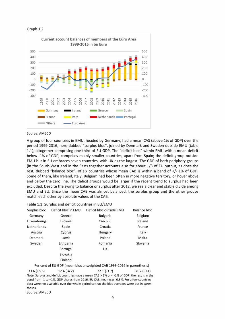
A group of four countries in EMU, headed by Germany, had a mean CAS (above 1% of GDP) over the period 1999-2016, here dubbed “surplus bloc”, joined by Denmark and Sweden outside EMU (table 1.1), altogether comprising one third of EU GDP. The “deficit bloc” within EMU with a mean deficit below -1% of GDP, comprises mainly smaller countries, apart from Spain; the deficit group outside EMU but in EU embraces seven countries, with UK as the largest. The GDP of both periphery groups (in the South-West and in the East) together accounts also for about 1/3 of EU output, as does the rest, dubbed “balance bloc”, of six countries whose mean CAB is within a band of +/- 1% of GDP. Some of them, like Ireland, Italy, Belgium had been often in more negative territory, or hover above and below the zero line. The deficit groups would be larger if the recent trend to surplus had been excluded. Despite the swing to balance or surplus after 2012, we see a clear and stable divide among EMU and EU. Since the mean CAB was almost balanced, the surplus group and the other groups match each other by absolute values of the CAB.
Table 1.1: Surplus and deficit countries in EU/EMU Surplus bloc Deficit bloc in EMU Deficit bloc outside EMU Balance bloc
Germany Greece Bulgaria Belgium Luxembourg Estonia Czech R. Ireland Netherlands Spain Croatia France
Austria Cyprus Hungary Italy Denmark Latvia Poland Malta Sweden Lithuania Romania Slovenia
Portugal UK
Slovakia
Finland
Per cent of EU GDP (mean bloc unweighted CAB 1999-2016 in parenthesis) 33.6 (+5.6) 12.4 (-4.2) 22.1 (-3.7) 31.2 (-0.1)
Note: Surplus and deficit countries have a mean CAB > 1% or < -1% of GDP, the rest is in the band from -1 to +1%. GDP shares from 2016. EU CAB mean was -0.3%. For a few countries data were not available over the whole period so that the bloc averages were put in paren-theses. Source: AMECO
-300
-200
-100
0
100
200
300
400
500
-300
-200
-100
0
100
200
300
400
500
1999
2000
2001
2002
2003
2004
2005
2006
2007
2008
2009
2010
2011
2012
2013
2014
2015
2016
Current account balances of members of the Euro Area 1999-2016 in bn Euro
Germany Ireland Greece Spain
France Italy Netherlands Portugal
Others Euro Area
9
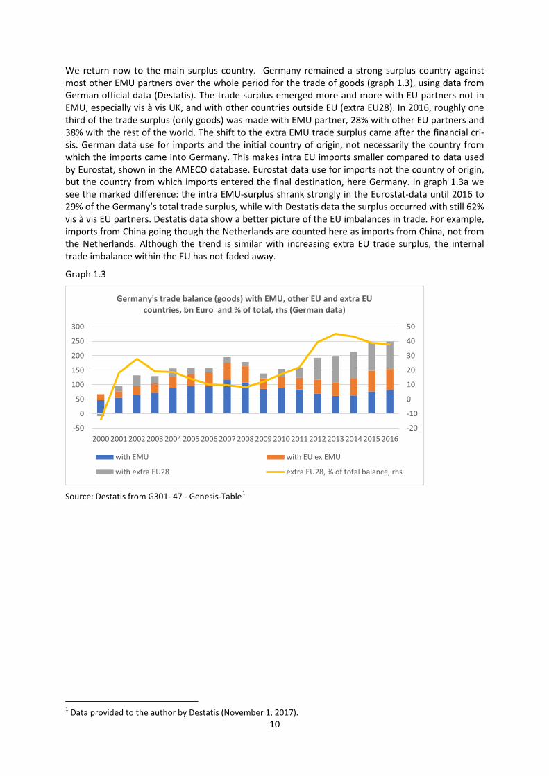
We return now to the main surplus country. Germany remained a strong surplus country against most other EMU partners over the whole period for the trade of goods (graph 1.3), using data from German official data (Destatis). The trade surplus emerged more and more with EU partners not in EMU, especially vis à vis UK, and with other countries outside EU (extra EU28). In 2016, roughly one third of the trade surplus (only goods) was made with EMU partner, 28% with other EU partners and 38% with the rest of the world. The shift to the extra EMU trade surplus came after the financial cri-sis. German data use for imports and the initial country of origin, not necessarily the country from which the imports came into Germany. This makes intra EU imports smaller compared to data used by Eurostat, shown in the AMECO database. Eurostat data use for imports not the country of origin, but the country from which imports entered the final destination, here Germany. In graph 1.3a we see the marked difference: the intra EMU-surplus shrank strongly in the Eurostat-data until 2016 to 29% of the Germany’s total trade surplus, while with Destatis data the surplus occurred with still 62% vis à vis EU partners. Destatis data show a better picture of the EU imbalances in trade. For example, imports from China going though the Netherlands are counted here as imports from China, not from the Netherlands. Although the trend is similar with increasing extra EU trade surplus, the internal trade imbalance within the EU has not faded away.
Graph 1.3
Source: Destatis from G301- 47 - Genesis-Table1
1 Data provided to the author by Destatis (November 1, 2017).
-20
-10
0
10
20
30
40
50
-50
0
50
100
150
200
250
300
2000 2001 2002 2003 2004 2005 2006 2007 2008 2009 2010 2011 2012 2013 2014 2015 2016
Germany's trade balance (goods) with EMU, other EU and extra EU countries, bn Euro and % of total, rhs (German data)
with EMU with EU ex EMU
with extra EU28 extra EU28, % of total balance, rhs
10

Graph 1.3a
Source: AMECO and Destatis from G301- 47 - Genesis-Table
Using the German data, the UK and the US are the biggest bilateral deficit countries against Germa-ny, accounting each for almost 20% of the German trade surplus in 2016 (without services)(Destatis 2017). Among the EU, Germany has the biggest bilateral surplus against France, and France’s deficit is mainly a bilateral one with Germany. For France, the bilateral deficit with Germany makes up 1.5% of its GDP (again without services).
Within EU, Germany has all the time concentrated its surpluses against the larger countries France, UK, Spain, Italy and against Austria (Destatis 2017). The German surplus against other mostly smaller EU countries is small in absolute numbers. France and Austria have sizable surpluses against other EU members which compensate more or less their deficit vis à vis Germany. Germany’s surplus against the GIIPS-countries (Greece, Ireland, Italy, Portugal and Spain) was at the peak of intra EMU imbal-ances in 2008 not more than 21% of Germany’s overall trade surplus (data only for trade with goods). It must be kept in mind that bilateral trade balances do not match necessarily bilateral net capital flows. Germany, together with France, invested huge amounts of finance in GIIPS assets, for Germa-ny around 20% of its GDP (cp. Chen et al. 2011, 39f.). France and also Germany received in 2008 huge financial inflows from the rest of the world (outside EMU) which were channelled to GIIPS as short-term finance.
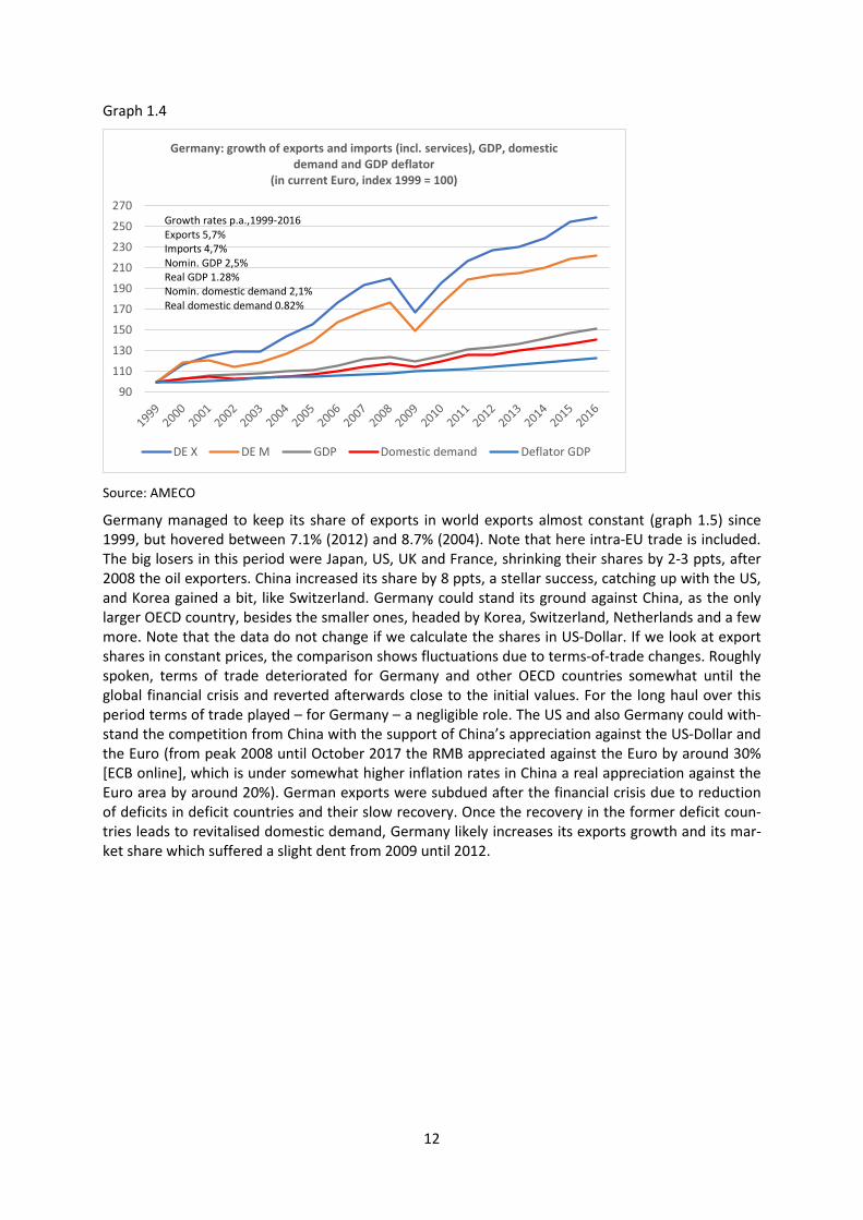
Since 2001, Germany’s exports of goods and services grew – in nominal values – continuously stronger than its imports (graph 1.4), except in 2009 when exports were hit more than imports. In the whole period 1999-2016, exports grew by 5.7% p.a., imports by 4.7%. The wedge between ex-ports and imports increased in absolute terms continuously. If we use another base year close to 1999, trend growth rates and the wedge between ex- and imports change insignificantly. As the trade and current account balance are expressed in nominal terms and related to the nominal GDP, the ratio is increasing also by low growth of nominal GDP, based on both low real GDP growth and below-target inflation (1.2% p.a. GDP deflator). Nominal domestic demand grew only by 2.1% p.a., and real domestic demand by not more 0.8% p.a. Low GDP and especially domestic demand growth dampened imports, while exports flourished alongside buoyant high world exports’ growth. Around one third of Germany’s real GDP growth was induced by the growth of the trade surplus, the rest by domestic demand (we discuss this in more detail in chapter 3). The low domestic demand trend came about despite only a small drop during the financial crisis and despite growth picking up after the crisis.
0
20
40
60
80
100
120
0
20
40
60
80
100
120
Germany's intra EU net exports, as percentage of total trade balance (goods, current prices), in German and EU data
(Destatis and AMECO)
Destatis: net intra -EU exports, % of trade balance
AMECO: net intra -EU exports, % of trade balance
11
Graph 1.4
Source: AMECO
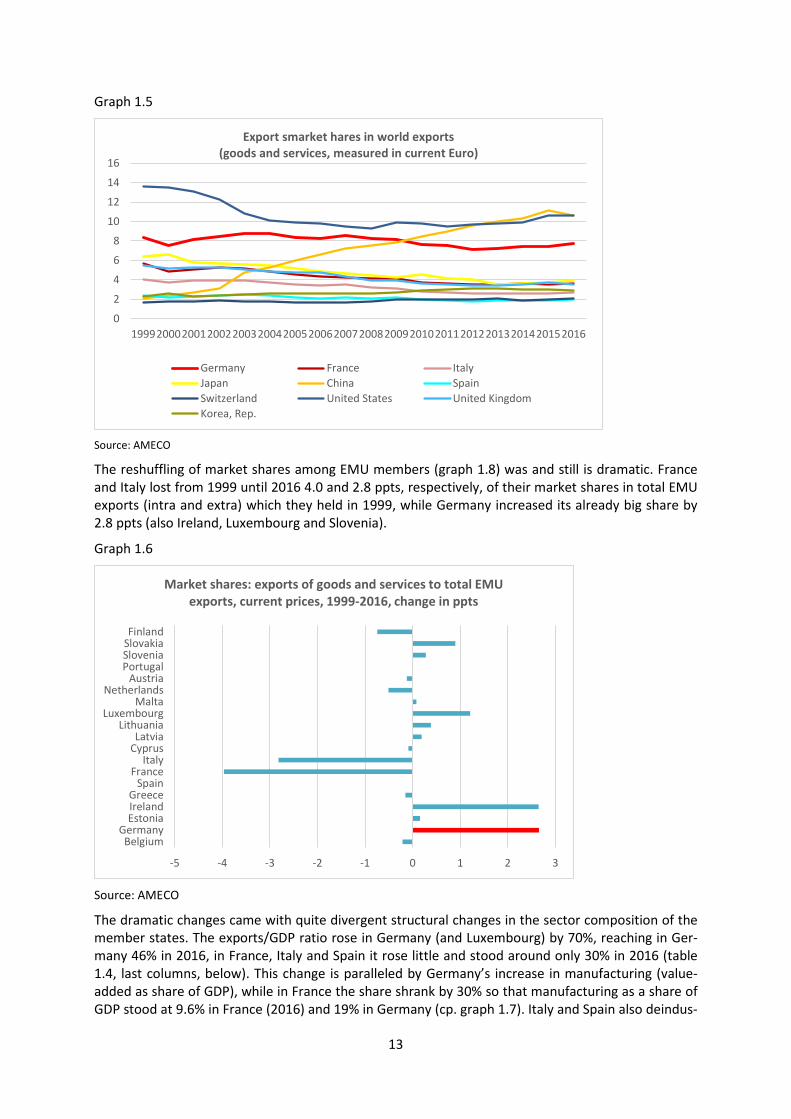
Germany managed to keep its share of exports in world exports almost constant (graph 1.5) since 1999, but hovered between 7.1% (2012) and 8.7% (2004). Note that here intra-EU trade is included. The big losers in this period were Japan, US, UK and France, shrinking their shares by 2-3 ppts, after 2008 the oil exporters. China increased its share by 8 ppts, a stellar success, catching up with the US, and Korea gained a bit, like Switzerland. Germany could stand its ground against China, as the only larger OECD country, besides the smaller ones, headed by Korea, Switzerland, Netherlands and a few more. Note that the data do not change if we calculate the shares in US-Dollar. If we look at export shares in constant prices, the comparison shows fluctuations due to terms-of-trade changes. Roughly spoken, terms of trade deteriorated for Germany and other OECD countries somewhat until the global financial crisis and reverted afterwards close to the initial values. For the long haul over this period terms of trade played – for Germany – a negligible role. The US and also Germany could with-stand the competition from China with the support of China’s appreciation against the US-Dollar and the Euro (from peak 2008 until October 2017 the RMB appreciated against the Euro by around 30% [ECB online], which is under somewhat higher inflation rates in China a real appreciation against the Euro area by around 20%). German exports were subdued after the financial crisis due to reduction of deficits in deficit countries and their slow recovery. Once the recovery in the former deficit coun-tries leads to revitalised domestic demand, Germany likely increases its exports growth and its mar-ket share which suffered a slight dent from 2009 until 2012.
90
110
130
150
170
190
210
230
250
270
Germany: growth of exports and imports (incl. services), GDP, domestic demand and GDP deflator
(in current Euro, index 1999 = 100)
DE X DE M GDP Domestic demand Deflator GDP
Growth rates p.a.,1999-2016 Exports 5,7% Imports 4,7% Nomin. GDP 2,5% Real GDP 1.28% Nomin. domestic demand 2,1% Real domestic demand 0.82%
12
Graph 1.5
Source: AMECO
The reshuffling of market shares among EMU members (graph 1.8) was and still is dramatic. France and Italy lost from 1999 until 2016 4.0 and 2.8 ppts, respectively, of their market shares in total EMU exports (intra and extra) which they held in 1999, while Germany increased its already big share by 2.8 ppts (also Ireland, Luxembourg and Slovenia).
Graph 1.6
Source: AMECO
The dramatic changes came with quite divergent structural changes in the sector composition of the member states. The exports/GDP ratio rose in Germany (and Luxembourg) by 70%, reaching in Ger-many 46% in 2016, in France, Italy and Spain it rose little and stood around only 30% in 2016 (table 1.4, last columns, below). This change is paralleled by Germany’s increase in manufacturing (value-added as share of GDP), while in France the share shrank by 30% so that manufacturing as a share of GDP stood at 9.6% in France (2016) and 19% in Germany (cp. graph 1.7). Italy and Spain also deindus-
0
2
4
6
8
10
12
14
16
199920002001200220032004200520062007200820092010201120122013201420152016
Export smarket hares in world exports (goods and services, measured in current Euro)
Germany France ItalyJapan China SpainSwitzerland United States United KingdomKorea, Rep.
-5 -4 -3 -2 -1 0 1 2 3
BelgiumGermany
EstoniaIrelandGreece
SpainFrance
ItalyCyprusLatvia
LithuaniaLuxembourg
MaltaNetherlands
AustriaPortugalSloveniaSlovakiaFinland
Market shares: exports of goods and services to total EMU exports, current prices, 1999-2016, change in ppts
13
trialised, like others too, but not as much as France did. This raises the question whether Germany is over-industrialised and others overly deindustrialised, similar to UK and US.
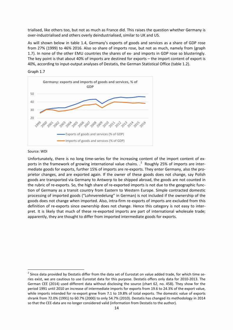
As will shown below in table 1.4, Germany’s exports of goods and services as a share of GDP rose from 27% (1999) to 46% 2016. Also so share of imports rose, but not as much, namely from (graph 1.7). In none of the other EMU countries the shares of ex- and imports in GDP rose so blusteringly. The key point is that about 40% of imports are destined for exports – the import content of export is 40%, according to input-output analyses of Destatis, the German Statistical Office (table 1.2).
Graph 1.7
Source: WDI
Unfortunately, there is no long time-series for the increasing content of the import content of ex-ports in the framework of growing international value chains. .2 Roughly 25% of imports are inter-mediate goods for exports, further 15% of imports are re-exports. They enter Germany, also the pro-prietor changes, and are exported again. If the owner of these goods does not change, say Polish goods are transported via Germany to Antwerp to be shipped abroad, the goods are not counted in the rubric of re-exports. So, the high share of re-exported imports is not due to the geographic func-tion of Germany as a transit country from Eastern to Western Europe. Simple contracted domestic processing of imported goods (“Lohnveredelung” in German) is not included if the ownership of the goods does not change when imported. Also, intra-firm re-exports of imports are excluded from this definition of re-exports since ownership does not change. Hence this category is not easy to inter-pret. It is likely that much of these re-exported imports are part of international wholesale trade; apparently, they are thought to differ from imported intermediate goods for exports.
2 Since data provided by Destatis differ from the data set of Eurostat on value added trade, for which time se-ries exist, we are cautious to use Eurostat data for this purpose. Destatis offers only data for 2010-2013. The German CEE (2014) used different data without disclosing the source (chart 62, no. 458). They show for the period 1991 until 2010 an increase of intermediate imports for exports from 19.6 to 24.3% of the export value, while imports intended for re-export grew from 7.1 to 19.8% of total exports. The domestic value of exports shrank from 72.0% (1991) to 60.7% (2000) to only 54.7% (2010). Destatis has changed its methodology in 2014 so that the CEE-data are no longer considered valid (information from Destatis to the author).
20
30
40
50
Germany: exports and imports of goods and services, % of GDP
Exports of goods and services (% of GDP)
Imports of goods and services (% of GDP)
14
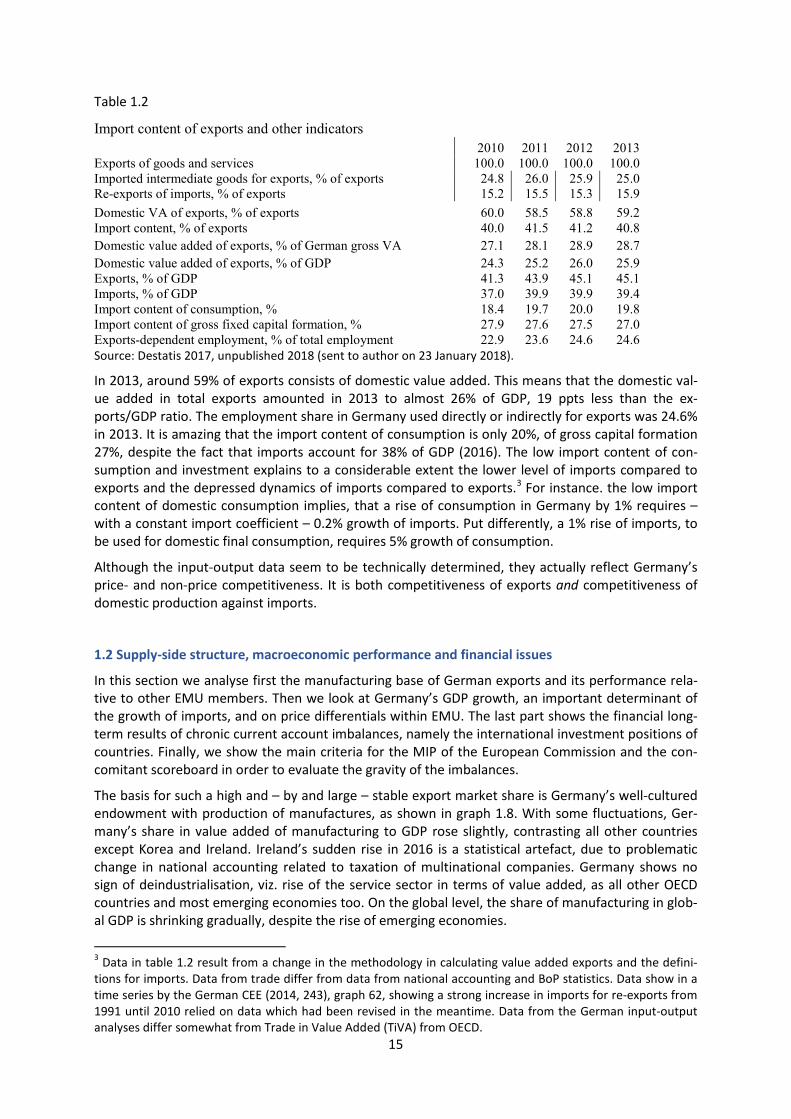
Table 1.2
Import content of exports and other indicators
2010 2011 2012 2013
Exports of goods and services 100.0 100.0 100.0 100.0 Imported intermediate goods for exports, % of exports 24.8 26.0 25.9 25.0 Re-exports of imports, % of exports 15.2 15.5 15.3 15.9 Domestic VA of exports, % of exports 60.0 58.5 58.8 59.2 Import content, % of exports 40.0 41.5 41.2 40.8 Domestic value added of exports, % of German gross VA 27.1 28.1 28.9 28.7 Domestic value added of exports, % of GDP 24.3 25.2 26.0 25.9 Exports, % of GDP 41.3 43.9 45.1 45.1 Imports, % of GDP 37.0 39.9 39.9 39.4 Import content of consumption, % 18.4 19.7 20.0 19.8 Import content of gross fixed capital formation, % 27.9 27.6 27.5 27.0 Exports-dependent employment, % of total employment 22.9 23.6 24.6 24.6 Source: Destatis 2017, unpublished 2018 (sent to author on 23 January 2018).
In 2013, around 59% of exports consists of domestic value added. This means that the domestic val-ue added in total exports amounted in 2013 to almost 26% of GDP, 19 ppts less than the ex-ports/GDP ratio. The employment share in Germany used directly or indirectly for exports was 24.6% in 2013. It is amazing that the import content of consumption is only 20%, of gross capital formation 27%, despite the fact that imports account for 38% of GDP (2016). The low import content of con-sumption and investment explains to a considerable extent the lower level of imports compared to exports and the depressed dynamics of imports compared to exports.3 For instance. the low import content of domestic consumption implies, that a rise of consumption in Germany by 1% requires – with a constant import coefficient – 0.2% growth of imports. Put differently, a 1% rise of imports, to be used for domestic final consumption, requires 5% growth of consumption.
Although the input-output data seem to be technically determined, they actually reflect Germany’s price- and non-price competitiveness. It is both competitiveness of exports and competitiveness of domestic production against imports.
1.2 Supply-side structure, macroeconomic performance and financial issues
In this section we analyse first the manufacturing base of German exports and its performance rela-tive to other EMU members. Then we look at Germany’s GDP growth, an important determinant of the growth of imports, and on price differentials within EMU. The last part shows the financial long-term results of chronic current account imbalances, namely the international investment positions of countries. Finally, we show the main criteria for the MIP of the European Commission and the con-comitant scoreboard in order to evaluate the gravity of the imbalances.
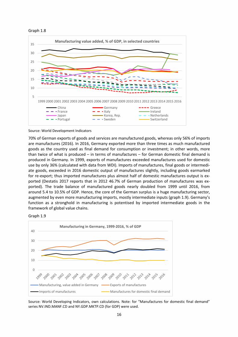
The basis for such a high and – by and large – stable export market share is Germany’s well-cultured endowment with production of manufactures, as shown in graph 1.8. With some fluctuations, Ger-many’s share in value added of manufacturing to GDP rose slightly, contrasting all other countries except Korea and Ireland. Ireland’s sudden rise in 2016 is a statistical artefact, due to problematic change in national accounting related to taxation of multinational companies. Germany shows no sign of deindustrialisation, viz. rise of the service sector in terms of value added, as all other OECD countries and most emerging economies too. On the global level, the share of manufacturing in glob-al GDP is shrinking gradually, despite the rise of emerging economies.
3 Data in table 1.2 result from a change in the methodology in calculating value added exports and the defini-tions for imports. Data from trade differ from data from national accounting and BoP statistics. Data show in a time series by the German CEE (2014, 243), graph 62, showing a strong increase in imports for re-exports from 1991 until 2010 relied on data which had been revised in the meantime. Data from the German input-output analyses differ somewhat from Trade in Value Added (TiVA) from OECD.
15
Graph 1.8
Source: World Development Indicators
70% of German exports of goods and services are manufactured goods, whereas only 56% of imports are manufactures (2016). In 2016, Germany exported more than three times as much manufactured goods as the country used as final demand for consumption or investment; in other words, more than twice of what is produced – in terms of manufactures – for German domestic final demand is produced in Germany. In 1999, exports of manufactures exceeded manufactures used for domestic use by only 36% (calculated with data from WDI). Imports of manufactures, final goods or intermedi-ate goods, exceeded in 2016 domestic output of manufactures slightly, including goods earmarked for re-export; thus imported manufactures plus almost half of domestic manufactures output is ex-ported (Destatis 2017 reports that in 2012 46.7% of German production of manufactures was ex-ported). The trade balance of manufactured goods nearly doubled from 1999 until 2016, from around 5.4 to 10.5% of GDP. Hence, the core of the German surplus is a huge manufacturing sector, augmented by even more manufacturing imports, mostly intermediate inputs (graph 1.9). Germany’s function as a stronghold in manufacturing is potentised by imported intermediate goods in the framework of global value chains.
Graph 1.9
Source: World Developing Indicators, own calculations. Note: for “Manufactures for domestic final demand” series NV.IND.MANF.CD and NY.GDP.MKTP.CD (for GDP) were used.
5
10
15
20
25
30
35
1999 2000 2001 2002 2003 2004 2005 2006 2007 2008 2009 2010 2011 2012 2013 2014 2015 2016
Manufacturing value added, % of GDP, in selected countries
China Germany GreeceFrance Italy IrelandJapan Korea, Rep. NetherlandsPortugal Sweden Switzerland
0
10
20
30
40Manufacturing in Germany, 1999-2016, % of GDP
Manufacturing, value added in Germany Exports of manufactures
Imports of manufactures Manufactures for domestic final demand
16
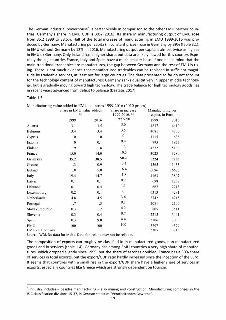
The German industrial powerhouse4 is better visible in comparison to the other EMU partner coun-tries. Germany’s share in EMU GDP is 30% (2016). Its share in manufacturing output of EMU rose from 35.2 1999 to 38.5%. Half of the total increase of manufacturing in EMU 1999-2016 was pro-duced by Germany. Manufacturing per capita (in constant prices) rose in Germany by 39% (table 3.1), in EMU without Germany by 12%. In 2016, Manufacturing output per capita is almost twice as high as in EMU ex Germany. Only Ireland has a higher share, but data are likely flawed for this country. Espe-cially the big countries France, Italy and Spain have a much smaller base. If one has in mind that the main traditional tradeables are manufactures, the gap between Germany and the rest of EMU is ris-ing. There is not much evidence that manufactured tradeables can be replaced in sufficient magni-tude by tradeable services, at least not for large countries. The data presented so far do not account for the technology content of manufactures; Germany ranks qualitatively in upper middle technolo-gy, but is gradually moving toward high technology. The trade balance for high technology goods has in recent years advanced from deficit to balance (Destatis 2017).
Table 1.3
Manufacturing value added in EMU countries 1999-2016 (2010 prices)
Share in EMU value added, %
Share in increase 1999-2016, %
Manufacturing per capita, in Euro
1999 2016 1999-201 1999 2016
Austria 3.1 3.5 5.0 4837 6410 Belgium 3.4 3.4 3.5 4081 4750 Cyprus 0 0 0 1115 638 Estonia 0 0.1 0.4 795 1977 Finland 1.9 1.8 1.3 4572 5166 France 15.0 14.0 10.5 3023 3280 Germany 35.2 38.5 50.2 5224 7283 Greece 1.3 0.9 -0.4 1565 1433 Ireland 1.8 5.0 16.4 6096 16676 Italy 19.4 14.7 -1.8 4163 3807 Latvia 0.1 0.1 0.2 698 1258 Lithuania 0.1 0.4 1.1 667 2213 Luxembourg 0.2 0.1 0 6313 4281 Netherlands 4.8 4.5 3.6 3742 4215 Portugal 1.7 1.3 0.1 2081 2109 Slovak Republic 0.3 1.2 4.2 805 3511 Slovenia 0.3 0.4 0.7 2215 3441 Spain 10.3 9.0 4.4 3106 3035 EMU 100 100 100 3797 4579 EMU ex Germany 3305 3713 Source: WDI. No data for Malta. Data for Ireland may not be reliable.
The composition of exports can roughly be classified in in manufactured goods, non-manufactured goods and in services (table 1.4). Germany has among EMU countries a very high share of manufac-tures, which dropped slightly since 1999, but the share of services doubled. France has a 30% share of services in total exports, but the export/GDP ratio hardly increased since the inception of the Euro. It seems that countries with a small rise in the export/GDP share have a higher share of services in exports, especially countries like Greece which are strongly dependent on tourism.
4 Industry includes – besides manufacturing – also mining and construction. Manufacturing comprises in the ISIC classification divisions 15-37, in German statistics “Verarbeitendes Gewerbe”.
17
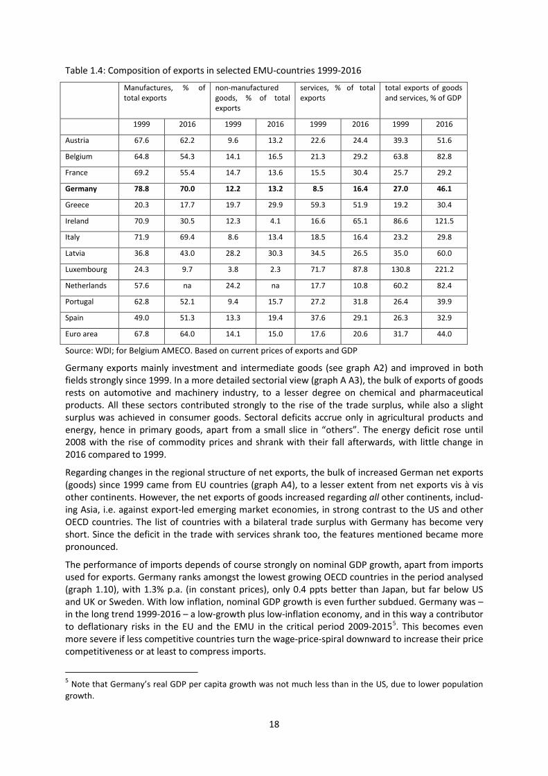
Table 1.4: Composition of exports in selected EMU-countries 1999-2016
Manufactures, % of total exports
non-manufactured goods, % of total exports
services, % of total exports
total exports of goods and services, % of GDP
1999 2016 1999 2016 1999 2016 1999 2016
Austria 67.6 62.2 9.6 13.2 22.6 24.4 39.3 51.6
Belgium 64.8 54.3 14.1 16.5 21.3 29.2 63.8 82.8
France 69.2 55.4 14.7 13.6 15.5 30.4 25.7 29.2
Germany 78.8 70.0 12.2 13.2 8.5 16.4 27.0 46.1
Greece 20.3 17.7 19.7 29.9 59.3 51.9 19.2 30.4
Ireland 70.9 30.5 12.3 4.1 16.6 65.1 86.6 121.5
Italy 71.9 69.4 8.6 13.4 18.5 16.4 23.2 29.8
Latvia 36.8 43.0 28.2 30.3 34.5 26.5 35.0 60.0
Luxembourg 24.3 9.7 3.8 2.3 71.7 87.8 130.8 221.2
Netherlands 57.6 na 24.2 na 17.7 10.8 60.2 82.4
Portugal 62.8 52.1 9.4 15.7 27.2 31.8 26.4 39.9
Spain 49.0 51.3 13.3 19.4 37.6 29.1 26.3 32.9
Euro area 67.8 64.0 14.1 15.0 17.6 20.6 31.7 44.0
Source: WDI; for Belgium AMECO. Based on current prices of exports and GDP
Germany exports mainly investment and intermediate goods (see graph A2) and improved in both fields strongly since 1999. In a more detailed sectorial view (graph A A3), the bulk of exports of goods rests on automotive and machinery industry, to a lesser degree on chemical and pharmaceutical products. All these sectors contributed strongly to the rise of the trade surplus, while also a slight surplus was achieved in consumer goods. Sectoral deficits accrue only in agricultural products and energy, hence in primary goods, apart from a small slice in “others”. The energy deficit rose until 2008 with the rise of commodity prices and shrank with their fall afterwards, with little change in 2016 compared to 1999.
Regarding changes in the regional structure of net exports, the bulk of increased German net exports (goods) since 1999 came from EU countries (graph A4), to a lesser extent from net exports vis à vis other continents. However, the net exports of goods increased regarding all other continents, includ-ing Asia, i.e. against export-led emerging market economies, in strong contrast to the US and other OECD countries. The list of countries with a bilateral trade surplus with Germany has become very short. Since the deficit in the trade with services shrank too, the features mentioned became more pronounced.
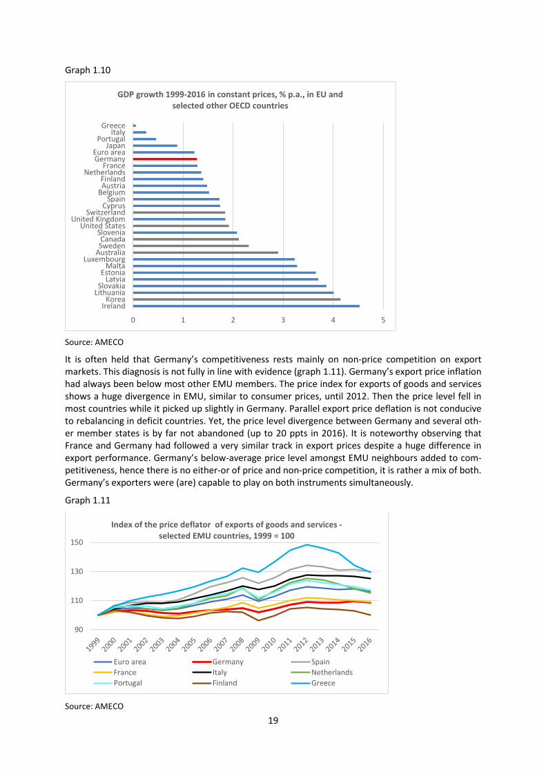
The performance of imports depends of course strongly on nominal GDP growth, apart from imports used for exports. Germany ranks amongst the lowest growing OECD countries in the period analysed (graph 1.10), with 1.3% p.a. (in constant prices), only 0.4 ppts better than Japan, but far below US and UK or Sweden. With low inflation, nominal GDP growth is even further subdued. Germany was – in the long trend 1999-2016 – a low-growth plus low-inflation economy, and in this way a contributor to deflationary risks in the EU and the EMU in the critical period 2009-20155. This becomes even more severe if less competitive countries turn the wage-price-spiral downward to increase their price competitiveness or at least to compress imports.
5 Note that Germany’s real GDP per capita growth was not much less than in the US, due to lower population growth.
18
Graph 1.10
Source: AMECO
It is often held that Germany’s competitiveness rests mainly on non-price competition on export markets. This diagnosis is not fully in line with evidence (graph 1.11). Germany’s export price inflation had always been below most other EMU members. The price index for exports of goods and services shows a huge divergence in EMU, similar to consumer prices, until 2012. Then the price level fell in most countries while it picked up slightly in Germany. Parallel export price deflation is not conducive to rebalancing in deficit countries. Yet, the price level divergence between Germany and several oth-er member states is by far not abandoned (up to 20 ppts in 2016). It is noteworthy observing that France and Germany had followed a very similar track in export prices despite a huge difference in export performance. Germany’s below-average price level amongst EMU neighbours added to com-petitiveness, hence there is no either-or of price and non-price competition, it is rather a mix of both. Germany’s exporters were (are) capable to play on both instruments simultaneously.
Graph 1.11
Source: AMECO
0 1 2 3 4 5
IrelandKorea
LithuaniaSlovakia
LatviaEstonia
MaltaLuxembourg
AustraliaSwedenCanada
SloveniaUnited States
United KingdomSwitzerland
CyprusSpain
BelgiumAustriaFinland
NetherlandsFrance
GermanyEuro area
JapanPortugal
ItalyGreece
GDP growth 1999-2016 in constant prices, % p.a., in EU and selected other OECD countries
90
110
130
150
Index of the price deflator of exports of goods and services - selected EMU countries, 1999 = 100
Euro area Germany SpainFrance Italy NetherlandsPortugal Finland Greece
19
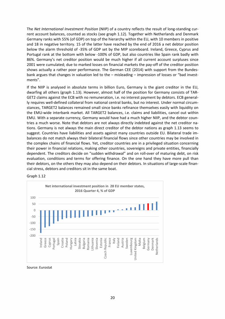
The Net International Investment Position (NIIP) of a country reflects the result of long-standing cur-rent account balances, counted as stocks (see graph 1.12). Together with Netherlands and Denmark Germany ranks with 55% (of GDP) on top of the hierarchy within the EU, with 10 members in positive and 18 in negative territory. 15 of the latter have reached by the end of 2016 a net debtor position below the alarm threshold of -35% of GDP set by the MIP scoreboard. Ireland, Greece, Cyprus and Portugal rank at the bottom with below -100% of GDP, but also countries like Spain rank badly with 86%. Germany’s net creditor position would be much higher if all current account surpluses since 2001 were cumulated; due to marked losses on financial markets the pay-off of the creditor position shows actually a rather poor performance. The German CEE (2014) with support from the Bundes-bank argues that changes in valuation led to the – misleading – impression of losses or “bad invest-ments”.
If the NIIP is analysed in absolute terms in billion Euro, Germany is the giant creditor in the EU, dwarfing all others (graph 1.13). However, almost half of the position for Germany consists of TAR-GET2 claims against the ECB with no remuneration, i.e. no interest payment by debtors. ECB general-ly requires well-defined collateral from national central banks, but no interest. Under normal circum-stances, TARGET2 balances remained small since banks refinance themselves easily with liquidity on the EMU-wide interbank market. All TARGET2 balances, i.e. claims and liabilities, cancel out within EMU. With a separate currency, Germany would have had a much higher NIIP, and the debtor coun-tries a much worse. Note that debtors are not always directly indebted against the net creditor na-tions. Germany is not always the main direct creditor of the debtor nations as graph 1.13 seems to suggest. Countries have liabilities and assets against many countries outside EU. Bilateral trade im-balances do not match always their bilateral financial flows since other countries may be involved in the complex chains of financial flows. Yet, creditor countries are in a privileged situation concerning their power in financial relations, making other countries, sovereigns and private entities, financially dependent. The creditors decide on “sudden withdrawal” and on roll-over of maturing debt, on risk evaluation, conditions and terms for offering finance. On the one hand they have more pull than their debtors, on the others they may also depend on their debtors. In situations of large-scale finan-cial stress, debtors and creditors sit in the same boat.
Graph 1.12
Source: Eurostat
-200
-150
-100
-50
0
50
100
Irela
ndGr
eece
Cypr
usPo
rtug
alSp
ain
Croa
tiaPo
land
Hung
ary
Latv
iaSl
ovak
iaBu
lgar
iaRo
man
iaLi
thua
nia
Slov
enia
Esto
nia
Czec
h Re
publ
icFr
ance
Italy
Finl
and
Aust
riaSw
eden
Luxe
mbo
urg
Uni
ted
King
dom
Mal
taBe
lgiu
mGe
rman
yDe
nmar
kN
ethe
rland
s
Net international investment position in 28 EU member states, 2016 Quarter 4, % of GDP
20

Graph 1.13
Source: Eurostat, TARGET2 balances from 8/2017, EC. Note: values for small countries not visible in the graph
Graph 1.14 shows the performance of the NIIP since the start of the Euro with a continuous increase for Germany and some other surplus countries against the downward movement for the deficit group, with France and Italy in the middle with a NIIP not far from zero. Germany’s position would be higher if there were no international “safe haven effect”. As this exists, Germany has many liabilities against these wealth owners. Five countries have moved deeply into negative territory, far below the MIP threshold of -35%.
Graph 1.14
Source: Eurostat
The bottom line of the analysis of the divergent NIIP in EMU is, firstly, that the trend is not sustaina-ble. Continued divergence tends to become explosive matter. The main debtors in the net debtor countries are governments and banks, to some extent also private households. Over-indebted com-panies can easily go bankrupt, not so governments, banks and households. Secondly, without TAR-GET2 and without zero-interest rate policy, including the large asset-purchasing programmes of the ECB, the divergence of NIIPs within EMU would have been much worse, also the net income balanc-es, in which interest payments are booked and which are part of the current account. It is quite likely that EMU without the strongly increasing TARGET2 balances during and after the financial crisis,
-1500
-1000
-500
0
500
1000
1500
2000
Spai
n
Irela
nd
Fran
ce
Italy
Gree
ce
Port
ugal
Slov
akia
Cypr
us
Lith
uani
a
Slov
enia
Latv
ia
Esto
nia
Mal
ta
Luxe
mbo
urg
Finl
and
Aust
ria
Belg
ium
Net
herla
nds
Germ
any
Net international investment position of EMU countries 2016, bn Euro
net debtors
net creditors
NIIP without TARGET2 balance
TARGET2 balance
-300
-200
-100
0
100
Net international investment positiom, % of GDP. in selected EMU countries (last quarter of year)
Belgium Germany Ireland GreeceSpain France Italy CyprusLuxembourg Netherlands Portugal Finland
21
functioning as lifesavers, EMU would have been blown apart. Thirdly, if interest rates return to nor-mal positive levels (in real terms), the private and public debt-overhang reflected in the highly nega-tive NIIP of several member countries, will become critical again.
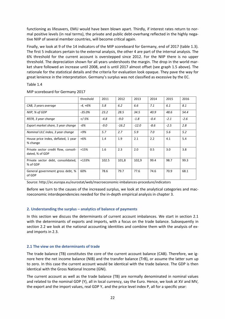
Finally, we look at 9 of the 14 indicators of the MIP scoreboard for Germany, end of 2017 (table 1.3). The first 5 indicators pertain to the external analysis, the other 4 are part of the internal analysis. The 6% threshold for the current account is overstepped since 2012. For the NIIP there is no upper threshold. The depreciation shown for all years undershoots the margin. The drop in the world mar-ket share followed an increase until 2008, and is until 2017 almost offset (see graph 1.5 above). The rationale for the statistical details and the criteria for evaluation look opaque. They pave the way for great lenience in the interpretation. Germany’s surplus was not classified as excessive by the EC.
Table 1.4
MIP scoreboard for Germany 2017
threshold 2011 2012 2013 2014 2015 2016
CAB, 3 years average -4, +6% 5.8 6.2 6.6 7.1 6.1 8.1
NIIP, % of GDP -35.0% 23.2 28.5 34.5 40.9 48.6 54.4
REER, 3 year change +/-5% -4.8 -9.0 -1.8 -0.4 -2.1 -2.6
Export market share, 5 year change -6% -9.0 -16.2 -12.0 -8.6 -2.5 2.8
Nominal ULC index, 3 year change +9% 5.7 2.7 5.9 7.0 5.6 5.2
House price index, deflated, 1 year % change
+6% 1.4 1.9 2.1 2.2 4.1 5.4
Private sector credit flow, consoli-dated, % of GDP
+15% 1.6 2.3 2.0 0.5 3.0 3.8
Private sector debt, consolidated, % of GDP
+133% 102.5 101,8 102,9 99.4 98.7 99.3
General government gross debt, % of GDP
60% 78.6 79.7 77.6 74.6 70.9 68.1
Source: http://ec.europa.eu/eurostat/web/macroeconomic-imbalances-procedure/indicators
Before we turn to the causes of the increased surplus, we look at the analytical categories and mac-roeconomic interdependencies needed for the in-depth empirical analysis in chapter 3.
2. Understanding the surplus – analytics of balance of payments
In this section we discuss the determinants of current account imbalances. We start in section 2.1 with the determinants of exports and imports, with a focus on the trade balance. Subsequently in section 2.2 we look at the national accounting identities and combine them with the analysis of ex- and imports in 2.3.
2.1 The view on the determinants of trade
The trade balance (TB) constitutes the core of the current account balance (CAB). Therefore, we ig-nore here the net income balance (NIB) and the transfer balance (TrB), or assume the latter sum up to zero. In this case the current account would be identical with the trade balance. The GDP is then identical with the Gross National Income (GNI).
The current account as well as the trade balance (TB) are normally denominated in nominal values and related to the nominal GDP (Y), all in local currency, say the Euro. Hence, we look at XV and MV, the export and the import values, real GDP Yr and the price level index P, all for a specific year:
22
CAB/Y = (TB + NIB + TrB)/Y
CAB/Y = TB/Y = (XV-MV)PYr if (NIB-TrB) = 0
The export value in local currency, say Euro, depends mainly on five independent variables: world income or global GDP (Yw), the price level of exports relative to prices of global exports (PX/W), the rest-of- the-world’s income propensity to import domestic goods (ßw), the real effective exchange rate (re)6 and the price elasticity of the volume of exports (εpX, absolute value).
(1) XV = f(Yw , PX/W , ßw , re, εpX)
The income propensity of the RoW (ßw) depends, inter alia, on the endowment of the economy with tradable goods or services (ET). Hence, we could write (with γ as a parameter)
(1a) ßw = γ(ET)
In oil-rich countries the availability of oil, in sun-rich countries the locations for tourism and in highly industrial countries the availability of tradable industrial goods, mainly manufacturing, as in the case of Germany. This endowment can change, but normally change occurs only gradually. It is also sub-ject to policies, like industrial policy and related other policies. Hinting to this type of endowment with tradables helps to include the supply side related preconditions for exports.
Since imports are measured here in local currency but denominated often in US-Dollar, the nominal exchange rate of the Euro against the US-Dollar ( e$€) has to be included as an independent variable. A stronger dollar reduces the value of imports in Euro. Furthermore, imports depend on domestic nominal GDP (YD), the ratio of the price level of local exports to those for similar goods on the world market (PX/W), the propensity to import goods needed as intermediate inputs for exports (ßx), the propensity to import goods needed for domestic final demand (ßD), the real effective exchange rate (re) and finally the price elasticity of imports (εpM). ßD depends – again and similar to equation (1a) – strongly on the endowment with tradables that tend to keep imports small.
(1b) MV = f(e$€, YD , Pw , ßx , ßD , re, εpM)
Of course, the imports considered here are the exports from the RoW for which equations (1) and (1a) are relevant, and conversely equation (1b) is the mirror image of equation (1) for the RoW. In both equations (1) and (1b) we have independent variables that determine directly the quantities of ex- or imports demanded, price-related variables and variables that characterise the preferences of demand for imports or for exports of a country, namely the income elasticities. The real exchange effects both exports and imports and is traditionally considered the most important variable to bal-ance trade and the current account. More precisely: if all other variables are constant, then the trade balance depends only on real exchange rates. Due to the often prevalent low price elasticity of ex-ports εpX and even more of imports, εpM , the effect of the real exchange rate on trade may be diluted or neutralised, at least the direct effect (see in more detail chapter 3). The price elasticity of exports (volume) for Germany is estimated at around 0.5, following econometric studies (Horn et al. 2017, even less in CEE 2014) so that the impact of real exchange rate changes remains very limited (other but similar estimations in Naastepad/Storm 2015, appendix). In other words, strong changes of the real exchange are necessary to impact the trade balance which are often observed in reality. There-fore, we should be cautious to belittle the relevance of real exchange rates. For the sake of simplicity, we assume that pricing to markets (PtM) does not occur; would it occur the effect of exchange rates is somewhat neutralised, at least in the short run. In case the neutralisation is only short-run since the adjustment to changed exchange rates needs time, we would have some kind of J-curve effect. The propensity of the rest of the world to import from the local economy and the propensity of the latter to import from RoW have evolved out of the – potentially divergent – technological and the sectorial structure of the economy and reflect also “technological competitiveness” and other forms
6 We use the direct quotation as with nominal exchange rates: local currency units per US-Dollar. A rise means depreciation. Likewise, this applies to the index of the real effective exchange rate.
23
of “structural” (non-price) competitiveness of exports such as specialising on exports to countries with above average output growth or on sectors facing high global growth. All this change the en-dowment with tradables which is behind the income propensity to import.
The main determinants of the trade balance are, focussing now on the ones selected as key features, as indicated in equation (1c). If the real exchange rate is widely diluted, excluding very strong ex-change rate changes, the three ßs are the heavyweights among the determinants of the trade bal-ance. We have included now for simplicity the terms of trade t, replacing PX/W and Pw from (1a) and (1b).
(1c) TB = f(ßw , ßx , ßD , t, re, εpX , εpM )
Now we turn to the dynamics of a surplus or deficit, viz. the growth rates of exports and imports. The growth of the nominal export value XV and the import value MV of a country are determined as fol-lows (^ stands for growth rate); the signs show the expected direction of the effects:
(2a) ^XV = f(yw , pX/W , εwy , rê, εpX) (2b) ^MV = f(e$€, yD , pw , πx , πD , rê, εpM)
+ + + + + - + - + + - +
For the (very) long run it can be concluded that the growth rates must converge, given a base year with a trade balance of nil, if explosive divergence is excluded. Note that equation (2c) is in line with stable growth of the trade balance in absolute terms, even if imports and exports do not balance to zero in the start period of the analysis. However, if the trade balance should be stable as a share of GDP, GDP would have to grow at the same pace. If this not the case, the trade balance to GDP ratio would explode if GDP grows slower than ex- and imports or diminish if GDP grows faster. Since in most countries and also worldwide trade grows faster than output, equation (2c) implies that the trade balance to GDP ratio tends to rise continuously if XV exceeds MV in the beginning of the analy-sis. The trade balance, in case not zero at the outset, would remain stable relative to GDP only if equation (2d) holds, viz. that domestic output grows (yD) as fast as trade.
(2c) ^XV = ^MV
(2d) ^XV = ^MV = yD (condition for constant trade balance to GDP ratio)
Explosive trade or current account surpluses, respectively, relative to GDP occur if
(3) ^XV = ^MV > yD with TB ≠ 0 in period t0, or if ^XV > ^MV > yD .
In chapter 3 we analyse the last inequality applied to Germany.
Equation (4) shows the determinants of the growth of the trade balance, ignoring here the TB to GDP ratio.
(4) ^TB = f(yw /yD , εwy/π, ^t, rê, εpX)
The growth rate of the export value depends mainly on the five independent variables shown in equation (4); in contrast to (1) and (1b), the independent variables have to be expressed as change rates: the growth rate of the nominal world income or global GDP (yw), the ratio of the export price deflator to the deflator of world exports (pX/W), the change of terms of trade (t), the world income elasticity7 of domestic exports (εwy), changes of the real effective exchange rate (rê)8, and again the price elasticity of the volume of exports (εpX, absolute value) assumed to be constant over time. We conjecture that the most important determinants for exports are the growth of demand for exports and the income elasticity of exports. Hence quantities, be they demand or supply driven, play a big-
7 The income elasticity expresses the per cent demand change for the demand for a good or, as here, for im-ports relative to the per cent change of income or GDP. Here we express the elasticities for changes in values, not in quantities as usually. Of, course, income elasticities can only be estimated if other determinants of ex- or imports are controlled for. 8 Again, we use the direct quotation as with nominal exchange rates as mentioned above.
24
ger role than prices, based on (price) “elasticity pessimism” as found in numerous empirical studies for Germany and other advanced countries with heterogeneous export goods. Again, this does not exclude that strong exchange rate changes matter. The may matter for the short or medium term, but continuous strong exchange rate changes are hardly imaginable.
Conversely, the growth of the value of imports depends again on the seven variables of equation (1b) but now shown as growth rates: the change nominal exchange rate of the Euro against the US-Dollar (ê$€), domestic nominal GDP growth (yD), the deflator for imports on the world market (pw), the elasticity of imports needed – as intermediate inputs – for exports (πx), the income elasticity of those imports that are needed for domestic final demand (πD), the change of the real exchange rate (rê) and finally the price elasticity of imports (εpM). Normally the most important independent variables are the growth of domestic demand and changes of both income elasticities mentioned. Again, we assume that real exchange rate changes have little traction on imports since econometric studies show that the price elasticity of imports is even smaller than the one for exports and continuous real strong exchange rate changes would be distortionary, especially if external debt is denominated in foreign currency.
Concentrating on the main determinants for exports and imports, the dynamics of the trade balance depends, as shown in equation (2d), on the ratio of domestic to world GDP growth and the ratio of the income elasticities for exports and imports, apart from the real exchange rate and the price elas-ticity. Changes of the terms of trade play normally only a temporary role.
The propensities to import, the ß’s in equations (1a) and (1b), have changed into income elasticities which play a key role together with growth differentials between trade partners. Income elasticities for exports capture “non-price competitiveness” of exports or sometimes dubbed “structural com-petitiveness” (Naastepad/Storm 2015, Storm/Naastepad 2015). Looking at the sectorial structure of exports, the income elasticities express the superiority or inferiority of export goods, regarding their demand abroad. What is produced rather than costs and prices matter in this view, especially in the long run. This includes the technology content and novelty of goods within a sector, but also the sec-torial structure of the exporting economy with respect to the intensity of demand. What is not cap-tured is the regional composition of export destinations regarding GDP growth. For the sake of keep-ing the analysis simple we neglect this item that also contributes to export growth, especially if ex-ports to emerging economies are taken into consideration. Conversely, this holds true for imports. The more inferior the goods imported are, or goods from industries with relative shrinking weights in the demand, the smaller the growth of imports. This however does not mean that such imports (or exports) are completely price inelastic. Insofar the often-used term “non-price competition” is mis-leading.
Income elasticities incorporate supply and demand side aspects. The supply side is related to tech-nology and innovation, monopoly, oligopoly and monopolistic competition, also to the size of firms involved in global trade, predominantly large firms, and – expressed more generally – changes in the endowment with tradeable goods or services. The demand side reflects aggregate demand from the side of importing countries and preferences of firms and consumers.
Note that our consideration of exports and imports does not explain whether the surplus causes the deficit or vice versa. Normally, the income elasticities and trend growth rates follow out of the histor-ical evolution of the country, corresponding to their stage of development and their structure of out-put. Most likely it is the combination of pull and push factors, difficult to be disentangled. Note also that we have excluded all problems of financing trade imbalances.
From functions (2a) and (2b) it seems at first glance logical that some advanced countries tend to have higher growth of exports than of imports, in particular if their production structure tends to produce goods more like smart phones and Porsche cars than like T-shirts and peanuts. And it is also likely that the GDP growth is smaller than trade growth. This would not only violate equation (2c), but lead to explosive growth of the trade balance to GDP ratio. However, it is evident that gaps be-tween exports and imports, positive or negative ones, are normally contained at some point. This
25
pertains predominantly to balance-of-payments-constrained growth (BoPCG), as analysed by Thirl-wall and others in the tradition of Kaldor.9 In the long run, most countries cannot carry high current account deficits, due to increased external indebtedness, and are limited in their capacity to depreci-ate (in real terms) their currency. In the long run, they have to balance imports and exports, normally by decreasing growth and thus compressing imports, or by structural change to improve export com-petitiveness and foster import substitution. Countries with BoPCG dampen exports of countries with excessive competitiveness. Countries with such “super-competitiveness” constrain other countries’ BoP and hence also their own growth of net exports. Another channel of reversing excessive deficits or surpluses could be huge exchange rate reversals, meaning excessive depreciation or appreciation, often accompanied by financial crises.
The limitation for current account surpluses lie both in the surplus country itself and in deficit coun-tries. An increasing surplus may be risky and disadvantageous for the surplus country itself. With own currency, it risks excessive appreciation at a certain point, and it would maximise net exports but not consumption, the final goal of growth. Yet, more compelling are the limitations for the deficit coun-tries stemming from growth beyond the BoP-constraints which leads to over-indebtedness, especial-ly in foreign currency if debt is denominated in the creditor’s currency. In a world with cross-border financial liberalisation, current account deficits can be financed more easily than earlier so that limi-tations are more elastic. Thirlwall assumes – mainly in regard to developing countries – very narrow limits for sustainable deficits. Intertemporal borrowing has to be paid back, requiring primary sur-plus. Permanent roll-over is ruled out.
Looking only at exports and imports when analysing the trade and current account balances neglects the role of GDP, domestic demand (often called absorption), specifically investment in the country under consideration, apart from other determinants of the independent variables, especially those impacting the real exchange rate. As mentioned, financing trade deficits was ignored so far.
2.2 The view on the determinants of saving and investment
Another approach to the analysis of BoP imbalances takes national accounting identities as the start-ing point. Most analyses use this approach, hence neglect the determinants of exports and imports.
Total national saving (S) is defined by the gross income earned (Y = Gross National Income (GNI)) minus consumption of private households and consumption of the government (recurrent spending without public investment). The rest of national spending of income for purchasing goods and ser-vices is for fixed investment of firms, including residential investment, and public investment (alto-gether I). If national saving exceeds national investment, excess saving is done abroad in the form of net capital exports. Net capital exports are identical with the current account balance. If we assume for the sake of simplicity that GDP = GNI, meaning that net foreign income and net transfers cancel out to zero, we can conclude:
(5) S-I = X-M = NKX > 0 (surplus country)
If this identity would be explained causally, which is implicitly or explicitly often done, we would write either
NX = S-I
9 “Thirlwall’s Law” states that the balance of payment constrained growth of a country is given by yB = εz/π = x/π (using Thirlwall’s notation). Income elasticity of exports is ε, z is world income growth, π is domestic income elasticity for imports and x is domestic export growth. This implies x = εz. Thirlwall assumes real exchange rate adjustments cannot occur permanently and that current accounts need to be in balance, apart from temporary deviations (Thirlwall 1979, McCombie/Thirlwall 2004). The authors conclude that the key mode of catching up for less developed countries constrained by their BoP is embarking on structural change with change of the income elasticities. The “Law” is however not limited to developing countries.
26
Meaning that X-M is seen as net exports NX (without distinguishing exports and imports) as being dependent on the variables on the right-hand side. If the net capital exports are considered the fun-damental cause of the trade balance, this causal interpretation would be written as
NX = NKX
Note that net capital exports NKX in modern economies are small relative to gross capital exports. More than 90% of gross capital exports have normally no impact on net capital exports, because they are pure financial flows into and out of the country which cancel out in the capital account.
A trade surplus (net exports NX) is identical with excess national saving over domestic investment, and also identical with net capital exports (NKX). The surplus economy produces more than it spends for goods and services; the over-production is sold to abroad, financed via net borrowing of the rest of the world from the net lending country. Running a surplus can now be interpreted as too high saving, relative to domestic investment, or too low investment relative to national saving, and rela-tive to the rest of the world. This implies that exports and their determinants are excluded in this equation, or considered as exogenously given. Imports are implicitly partially included as far as they are determined by domestic demand. All other independent variables of imports mentioned in (1b) are considered – implicitly – as given exogenously.
When we analyse the growth of the CAS of Germany, we conclude for equation (5) that the increase of S in a certain period (ΔS) exceeds the increase of investment (ΔI), and the increase of exports (ΔX) exceeds the increase of imports (ΔM); the increase of net capital outflows matches the increase of the trade surplus and the increase of foreign assets ΔFA exceeds the increase of liabilities to abroad, ΔFL. Hence, we can write
(6) Δ(S – I) = Δ(X – M) = Δ(FA – FL) > 0
If (S-I) is denoted as total national saving SN and FA-FL is net capital exports NKX (or increase of net foreign assets) we can write for the increase of the current account surplus in a certain period:
(6a) ΔCAS = ΔSN = ΔNX = ΔNKX = ΔNFA > 0
Equations (6) and (6a) do not show any causality. Many interpretations may be possible. It becomes even more open to different interpretations, if we include the mirror image equation for the rest of the world (denoted with *), which runs a current account deficit:
(7) SN + SN* = 0
Assume the home country, say Germany, has a national saving surplus SN, the rest of the world has a saving deficit SN*= (S*- I*) < 0). Does the surplus country cause the deficit abroad, or the net borrow-ing abroad the net lending in the home country? Normally it is a mutual causation, but reality may differ at times. The pull or push question may also depend on the type of capital flows (see below)
National saving is composed of net saving of private households SH, of the government, i.e. the budget balance SG (= T-G, i.e. a budget surplus if tax revenues T exceed spending G) and net saving of firms, SF (sometimes also called corporate saving or retained cash flow)). Saving in this context is a flow measure for the period, not the stock of savings. Total investment stems from firms IF, from residential investment IR and from public investment IG. Now we can write
(8) (SH + SG + SF) – (IF + IR + IG) = NX = - SN*
All sectorial savings add up to zero if the foreign sector is included:
(9) (S-I) - NX = 0 or for the increments Δ(S-I) – ΔNX = 0
NX is equal to negative total foreign saving which can be split in its different components as well.
It is noteworthy to mention that all identities shown reflect ex post values for the end of a period. The identities tell us nothing about exports and only little about imports and their respective deter-minants. Net exports seem to result out of domestic saving and investment when reading equation
27

(8) from the left to the right side. National income is obviously assumed as given, also net income of the rest of the world. Rebalancing a surplus requires higher domestic absorption of output, i.e. more (C+I+G) alias more domestic demand, and rebalancing a deficit needs cutting back consumption and/or investment, often called austerity in a broader sense (including wage and fiscal austerity). Adjustments come symmetrically from both sides or asymmetrically, with focus either on the surplus or the deficit countries.
The widespread reading of equation (7) and (8) is that deficit countries live beyond their means and should save more, in particular regarding wages and budget balances. Thrift of the surplus country is the virtue, profligacy the vice of the deficit country. Yet, pushing the deficit countries toward more thrift would make the surplus countries less thrifty as their surplus vanishes – and they would have to abandon their virtue. Obviously, this “moral” reasoning is incoherent. Making excessive surpluses or deficits are two forms of vices. The remaining question is what “excessive” means.
The alternative narrative would be that the surplus country is obsessed with excessive thriftiness, addicted to irrational saving, pushing other countries in – at least partially – involuntary deficits. This obsession may take the form of a kind of outright or hidden mercantilism, causing a “saving glut”10 and accumulating financial wealth rather than spending it for real investment and ultimately con-sumption.
Current account and increasing income distribution
Equation (8) can also be explained by changes in income distribution as proposed in recent literature. If there is an increase in income inequality as observed in many OECD countries over the last dec-ades, especially in the early 2000s, it can impact the current in different directions. If the top income earners start to increase their consumption further, while income groups below the top one attempt to keep up with upper rank in terms of consumption, a cascade of consumption unfolds which reach-es also the low-income groups. Many in the lower income strata indulge in credit-based consump-tion. Rising profits of corporations are predominantly distributed to shareholders. Subsequently a consumption-led growth performance with increased proclivity for imports ensues. This narrative seems to hold true to some extent for explaining the falling current account balance in the US; it contributes also to explaining the financial crisis of 2007-9 (cp. Behringer et al. 2013, van Treeck 2014),
Following the recent literature (for an overview cp. Behringer/van Treeck 2015, Beh-ringer/Theobald/van Treeck 2017), increased income inequality may be more likely to suppress do-mestic demand, dampen growth, reduce imports and bolster saving of the middle and top income groups with higher saving propensity. A special focus is laid on countries like Germany, where the shift in the functional income distribution in favour of profits and wealth income leads to higher re-tained profits of corporations. The consumption cascade does not occur. Shareholders accept the increase of corporate saving which is often saved in geographically diversified portfolios. From this perspective, the saving of firms (SF in equation 8) is an important driver for the increase of national saving. In section 3 we will see that this is indeed the predominant for increased overall saving in Germany in the period 1999-2016. The effect of the more unequal income distribution on the current is reinforced if the more inequality dampens growth and hence imports.
The link between functional income distribution which also changes the personal income distribution at the primary level (without fiscal redistribution) was addressed early by Kalecki and post-Kaleckian scholars (cp. Hein 2014). The basic rationale is that the profit share increases the higher the trade surplus, at a given national income. That the increased profit share is needed to let the trade surplus materialise via S > I and ensuing net capital exports is the other side of the coin, not directly ad-dressed by Kalecki. PR are profits of firms, CC is consumption of capitalists, i.e. shareholders, SW is saving of workers, as shown in equation (8a).
10 Note that concepts of a “global saving glut”, as held by Greenspan/Bernanke, Summers or von Weizsäcker (2016), mainly focus on stocks of savings but at times confuse flows and stocks or switch between them.
28
(8a) PR = I + CC – SW + G-T + X-M
The underlying assumptions are that the only costs of production are wages (for simplicity) and that the saving ratio of capitalists is than the one of workers. Then profits would – in a closed economy with balanced budget – depend solely on the demand of capitalists for their own output, if workers would consume what they earn. If the latter save more out of wages, profits shrink, unless compen-sated by demand from government deficits and/or by demand from abroad, i.e. a trade surplus. In-creased functional income distribution with retained profits, hence constrained increase of share-holders’ consumption, requires then a rise in the trade (or current account) balance. It is likely that such export-led growth is lower than domestic-demand led growth, unless the export multiplier is very high.
For strongly export-led economies the Kaleckian case seems logical. The model can be augmented and modified in many directions.
The absorption approach to BoP rebalancing
The spending approach to BoP imbalances with its focus on national saving and investment can be used for concepts of rebalancing based on the so-called absorption approach. Absorption A is the sum of domestic final demand, namely A = C+I+G. Absorption can also be understood as output mi-nus the trade balance: A = Y –(X-M). Under a fixed exchange rate regime, a trade deficit implies that absorption exceeds output (A > Y), and a trade surplus means that output exceeds absorption (Y > A).
For the deficit country, expenditure reducing policy could be advised, by which with fiscal or mone-tary policy the absorption is reduced relative to output. This kind of austerity policy is likely to bal-ance BoP at the expense of generating or increasing unemployment and aggravating the negative output gap. This implies deflationary risks. Nothing would be achieved if output and absorption drop in tandem. To avoid or attenuate this policy, the chronic surplus countries should follow expenditure switching policy. This means increasing absorption by fiscal or other policies relative to output but with increasing output – if actual output is below potential output. If full (or equilibrium) employ-ment is already reached and the output gap has vanished, expenditure switching policy would induce higher inflation. This would raise the real exchange rate thus dampening exports and increasing im-ports, assuming that the Marshall-Lerner condition (MLC)11 is satisfied. In turn this gives deficit coun-tries the chance to reduce absorption and increase output via more net exports, based on real de-preciation. This is basically James Meade’s (1951, 1955) two-pronged approach to BoP-rebalancing with a mix of expenditure reducing and expenditure switching policies. The absorption approach to BoP imbalances stands in contrast to the so-called elasticity approach, which rests solely on exchange rate adjustments via flexible nominal exchange rates. However, there is a trade-off between inflation and external equilibrium. Meade did not pay attention to the issues of possibly weak structural com-petitiveness with limited price elasticities for exports and imports and hence limited effectiveness of real exchange rate adjustments. Yet, the basic ideas are still valid.
In this section we started from the well-known identities elaborated in National Accounting. We end-ed in different interpretations. Understanding the identities is important, but important issues re-main invisible from this angle, especially exchange rates, capital flows and the other variables men-tioned in the context of trade in section 2.1., pertaining to the determinants of exports and imports. Causal interpretations should be done with caution. We turn now to combining the approaches via trade determinants and those focusing on national saving and investment.
11 The MLC requires perfect supply elasticity of trading countries and demand elasticities for exports and im-ports whose sum is (in absolute terms) > 1.
29
2.3 Combining the trade and the saving view
In this chapter we integrate in the first part the approaches described above in sections 2.1 and 2.2. In the second part we discuss constraints for deficit countries in running external deficits.
Combined approach
The starting point is equation (5), namely
X-M = S – I
We assume that X is exogenous in a given period when the determinants identified above are con-sidered as given. Of course, all independent variables can change, but for the time being the world demand for goods as well as the capacity to produce goods that are demanded, reflected in the in-come elasticity, do not change quickly. M is to some extent earmarked for exports, say M1, while the rest of M depends on the domestic demand DD (DD=I+C+G) in the home country whose current ac-count we analyse. We call this parts of imports M2. On the right-hand side of the equation, gross investment (gross capital formation) depends on a number of variables, for instance the real interest rate r, degree of capacity utilisation or the output gap OG, expected final demand eFD for (C, G, X), the age of the capital stock a, representing the perceived need to replace old vintages, profit expec-tations ep, and animal spirits, as, reflecting the degree of uncertainty. Of course, the determinants for the different types of investment – corporate investment, residential and public investment – differ; s2 represents fiscal policy.
For investment I (gross capital formation) we write
(10) I =f((r, ep, eFD, OG, a, s2, as)
or I(Z)
whereby Z captures all the complex variables in (10).
How about S? S comprises the saving of households, the government (viz. the budget balance) and the saving of firms as retained cash flow. This means there are three saving propensities s1, s2 and s3, aggregated as s = S/Y. Hence these saving propensities determine by and large C and G, and partly also I and M2. It is important to take net exports not as one variable, as was done in equations (5-9) since exports and imports are determined by quite different factors. For a causal analysis this differ-entiation is necessary, for showing identities not.
(11) X-M1-M2 = (s1+s2+s3)Y – I(Z)
Since X-M=s(Y)–I, we can write for Y
(12) Y = (I[Z] + X-M1[X]-M2[DD]) /(s1+s2+s3)
Now we can conclude. The growth of the current account depends in equation (1) mainly on the ex-ogenous growth of exports, ^X (we omit here for the sake of brevity the acronym for value, as men-tioned in equation (1a)), and the growth of M2, strongly dependent on the growth of domestic de-mand including I(Z). Note that various policy tools are inside some of the independent variables, such a fiscal policy in s2, policies regarding income distribution, affecting s1, various factors inside Z, such as policy for housing investment, monetary policy, taxation of profits etc. It is necessary to emphasize that M2 depends strongly on s (in all three forms), but also on the growth of GDP, more precisely real GDP and the inflation rate. A higher inflation rate might increase the value of imports if some degree of pricing to markets exists, but inflation also impacts nominal GDP, the denominator of the current account to GDP ratio.
Of course, exogenising exports, often the most dynamic factor for the current account, is not tena-ble, neither must finance be omitted. In a simple 2-country model with country G and country RoW, G’s exports are RoW’s imports (if * denotes RoW: M* = X, X* = M), and G’s imports ore RoW’s ex-ports. This implies that exports of each country depend on domestic demand in the other country. Hence, the generation of high domestic demand in both countries tends to generate strong exports
30
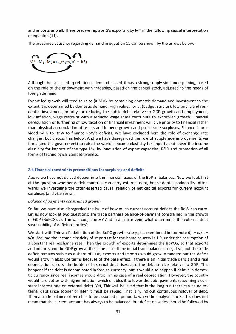
and imports as well. Therefore, we replace G’s exports X by M* in the following causal interpretation of equation (11).
The presumed causality regarding demand in equation 11 can be shown by the arrows below.
Although the causal interpretation is demand-biased, it has a strong supply-side underpinning, based on the role of the endowment with tradables, based on the capital stock, adjusted to the needs of foreign demand.
Export-led growth will tend to raise (X-M)/Y by containing domestic demand and investment to the extent it is determined by domestic demand. High values for s2 (budget surplus), low public and resi-dential investment, priority for reducing the public debt relative to GDP growth and employment, low inflation, wage restraint with a reduced wage share contribute to export-led growth. Financial deregulation or furthering of low taxation of financial investment will give priority to financial rather than physical accumulation of assets and impede growth and push trade surpluses. Finance is pro-vided by G to RoW to finance RoW’s deficits. We have excluded here the role of exchange rate changes, but discuss this below. And we have disregarded the role of supply side improvements via firms (and the government) to raise the world’s income elasticity for imports and lower the income elasticity for imports of the type M2, by innovation of export capacities, R&D and promotion of all forms of technological competitiveness.
2.4 Financial constraints preconditions for surpluses and deficits
Above we have not delved deeper into the financial issues of the BoP imbalances. Now we look first at the question whether deficit countries can carry external debt, hence debt sustainability. After-wards we investigate the often-asserted causal relation of net capital exports for current account surpluses (and vice versa).
Balance of payments constrained growth
So far, we have also disregarded the issue of how much current account deficits the RoW can carry. Let us now look at two questions: are trade partners balance-of-payment constrained in the growth of GDP (BoPCG), as Thirlwall conjectures? And in a similar vein, what determines the external debt sustainability of deficit countries?
We start with Thirlwall’s definition of the BoPC growth rate yB (as mentioned in footnote 6): = εz/π = x/π. Assume the income elasticity of imports π for the home country is 1.0, under the assumption of a constant real exchange rate. Then the growth of exports determines the BoPCG, so that exports and imports and the GDP grow at the same pace. If the initial trade balance is negative, but the trade deficit remains stable as a share of GDP, exports and imports would grow in tandem but the deficit would grow in absolute terms because of the base effect. If there is an initial trade deficit and a real depreciation occurs, the burden of external debt rises, also the debt service relative to GDP. This happens if the debt is denominated in foreign currency, but it would also happen if debt is in domes-tic currency since real incomes would drop in this case of a real depreciation. However, the country would fare better with higher inflation which enables it to lower the debt payments (assuming a con-stant interest rate on external debt). Yet, Thirlwall believed that in the long run there can be no ex-ternal debt since sooner or later it must be repaid. That is ruling out continuous rollover of debt. Then a trade balance of zero has to be assumed in period t0 when the analysis starts. This does not mean that the current account has always to be balanced. But deficit episodes should be followed by
31
surplus phases. This precondition requires that countries increase x by increasing ε, meaning mod-ernising the export structure toward goods (or destinations of exports) with stronger external de-mand. This is a simple and clear answer to the problem, but normally not easy to implement. In the end the issue boils down to the question of sustainability of external debt, which includes the ques-tion whether rollover risks should be accepted.
Debt sustainability
Let us now check the external debt sustainability using the normal arithmetic for public debt sustain-ability in the sense that that the debt burden and the debt service relative to GDP stay constant over time as a trend, occasional deviations not excluded. The well-known restriction is as follows. To hold the debt-GDP-ratio d constant over time, whatever its value, a primary balance p – budget balance without interest payments as share of GDP – is needed which depends on the difference of the real growth rate of GDP yr and the real interest rate r12:
p = (yr-r)d
Translating this restriction into the BoP implies that the CAB is equivalent to the entire budget bal-ance, the primary balance equivalent to the trade balance, interest payments on external debt corre-spond to the net income balance (other items excluded, also transfers), and the debt is represented in the net international investment position NIIP (cp. Priewe 2011, 23f.). If the latter is negative, in-terest has to be paid on net debt outstanding. Now we can write for the trade deficit (here with a positive sign, i.e. M-X) and all variables in nominal terms because the trade balance and NIIP are normally expressed in nominal values; y is now growth of nominal output Y, and i stands for the nom-inal interest rate on external debt, replacing r:
(13) (M-X)/Y = (y-i)NIIP/Y
Stabilising NIIP requires under y = i a balanced trade balance. This implies that the current account is initially negative if the NIIP/Y < 0, to the extent of the debt service. If y exceeds i, a higher trade defi-cit is sustainable even over the long run. Even if the trade balance were zero, but NIIP strongly in deficit, the debt service would have to be transferred out of the national income year by year. In case of zero external debt, stabilising this level requires also a zero-trade balance (or a surplus).
Let as assume that NIIP stands at -35% of GDP, the threshold in MIP set by the EC. Stabilising external debt at a real interest rate of 2%, real growth of 3% and 2% target inflation (hence i=4%, y=5%) al-lows a trade deficit of not more than 0.35%. This applies also if external debt is paid in own or a common currency. A one-time depreciation of the real exchange rate would require a higher debt service, hence higher net income balance deficit. It might also signal a higher risk premium on inter-est rates. It has to be emphasised again that this approach assumes that either debt or equity finance is used continuously for financing the profit transfer; if in case of equity financing profits or returns on equity like dividends are reinvested in the countries, the income balance improves. Transfers like remittance inflows etc. allow easier payment of the debt service. As we saw in graph 1.11 on NIIP in EMU, debt sustainability considerations had been completely ignored in the GIIPS-group (except Ita-ly) when NIIP worsened so strongly since 1999 (see graph 1.13).
An improving (less negative) NIIP requires smaller trade deficits in the future or trade surpluses, or transfers from abroad, debt relief or debt restructuring. The point we want to make here is that the debt service can possibly be paid out of the GNI of a country, like a continuous transfer of national income to other countries. At the same time running further trade deficits increases the debt burden and necessitates for future generations rising transfers for debt payment, like taxing of the surplus countries. It makes a big difference if a country is highly indebted vis à vis own residents – it is paid “to ourselves”, say to resident banks which need the liquidity. External debt constraints can be alle-
12 The equation for the budget constraint is derived as follows. The primary budget deficit is P: P = (G-T-iD), To keep D/Y = d constant, ^D = ΔD/D = ΔY/Y= y, growth of D must match output growth y. P = (ΔY/Y)D - iD . Ex-pressing P relative to Y, i.e. P/Y = p, we get p = (y-i)d.
32
viated, if it occurs as liability to the ECB within the TARGET2 payment system of EMU, without remu-neration. Although TARGET2 is not designed as a way to alleviate the burden of intra EMU imbalanc-es, it has a positive function in this respect. This is emphasised by authors who interpret the EMU payment system similar to Keynes’s idea for a clearing union (Lavoie 2015).
Special conditions for debt sustainability in a monetary union?
Let us discuss for a moment the notion that BoP issues in a monetary union become irrelevant, like they become irrelevant in a federal state with deficit and surplus regions. This notion was implicit in the concepts of the Werner Plan for a European monetary union in the early 1970s, and it reap-peared in the design of the Maastricht Treaty where all issues on current account were disregarded. A common currency as in EMU allows financing of net imports with own currency, an enormous ad-vantage compared to countries compelled to be indebted in foreign currency, typically developing and emerging economies. This implies that finance for trade can be generated by domestic banks, if not financed out of current income. For some observers, this boils down to handling external debt of EMU members as a microeconomic issue like handling debt for any kind of debtor (Collignon 2017). Of course, creditors as well as debtors must be attentive vis à vis their counterparts, as always. Put differently, external debt mutates to debt of regions, not nations. To some extent this is true. Yet, the debt analysis shown above is valid also for regions which then can be aggregated to nations. We hold that this view is misleading and undervalues he risks of EMU imbalances. The reasoning goes as follows.
Assume that in a country with a big sector of the private economy exports fall short of imports so that also national net exports are continuously negative. It is more spent for consumption and in-vestment than produced. The level of over-spending relative to income can only be financed by bank credit. Banks can refinance themselves on the European interbank market or directly at the ECB if valid collateral can be offered, normally government bonds or treasury bills or similar. After some time of continuous debt financing collateral might become scarce, so that external debt financing on financial markets has to be used. In this scenario the NIIP falls, becomes negative, more and more – unless GDP rises faster than the interest rate. See above. If this is not the case, the government and the banks can even become illiquid if the ECB refuses the collateral and private creditors refuse the roll-over of maturing old debt and also reject new lending. This leads to insolvency of banks and “bankruptcy” of the government, since the ECB is no full lender of last resort as in traditional nation states. Would the ECB become a normal lender of last resort as in all OECD states with debt in own currency, monetary financing or something akin to it would at least avoid illiquidity and ensuing in-solvency. In sum, the microeconomic view in which individual debt seems innocuous, since over-indebted borrowers can default without nationwide repercussions, does not hold if too many, includ-ing banks, tend to default. Hence, the proposition that external debt in EMU members is without risks, turns out to be a fallacy of aggregation.
This reasoning can be supported by looking at regional development. If a structurally weak region spends more than it produces, taken all sectors including regional states, cities, townships, enterpris-es and households together, the “agents” in the region will have to cut expenditures sooner or later or become over-indebted and go bankrupt; employment falls, out-migration is likely – unless a cen-tral fiscal entity offers transfers or credit or debt relief. This is a scenario of fiscal federalism which however does not exist on the level of the EU or EMU, apart from the small EU budget with a volume of 1% of EU GDP.
Another variant of disregarding current accounts in EMU follows implicitly the Lawson Doctrine13. Only public deficits and debt need to be controlled with sustainability criteria, but not private deficits
13 The “Lawson doctrine” is named after Nigel Lawson, the Chancellor of the Exchequer in the United Kingdom who articulated it in the 1980s. The doctrine holds that current account imbalances, as far as they are caused by private saving and investment, based on rational expectations and as far as no other distortions exist, should not be subject to public interventions.
33
and debt. Private debtors tend to behave under competition rationally and avoid illiquidity and bank-ruptcy; if not, they go bust and should go bust as a natural consequence of functioning markets. If the majority of firms behaves exuberantly, over-lending of banks may be involved which requires better surveillance of banks, micro- and macroprudential regulation. This sounds logical, but history has shown so far that banking regulations are mostly insufficient, can be bypassed by shadow banks or impeded by legacy debt from the past. The basic underlying problem, namely problematic funda-mentals with balance-of-payments-constrained growth, weak non-price competitiveness, etc. “Inter-nal devaluation” might allow current account balance via compressed imports, at the expense of internal disequilibrium with unemployment and deflationary risks. Furthermore, a limited look at deficit/debt criteria of the EMU/EU for the government budget has no direct bearing for the current account. If the public deficit is high, say above 3% of GDP, it may be irrelevant for the current account if other sectors, e.g. private households, save sufficiently. Or under high private sector deficits, a 3% public deficit may be too much. Conversely for surplus countries: a balanced budget can increase the surplus, if the private sector is in surplus too. Even if deficit countries keep their current accounts deficits well under control, excessive surpluses in the surplus bloc of EMU will lead to a current ac-count surplus of EMU against other countries outside EMU. Sustainability of the NIIP should also be considered by surplus countries. In short, current account imbalances within a monetary union need special policies, in particular if labour mobility is low and fiscal federalism does not exist. Rules for the public budget and banking regulation are no sufficient substitutes.
The conclusion of our considerations on BoPCG and debt sustainability is that countries are well ad-vised to keep their trade deficits small and avoid decreasing NIIP. Countries running temporarily defi-cits for some years but benefit from positive NIIP have much more leeway.
The role of net capital exports
Let us finally turn to an issue which has brought much confusion. From National Accounting it follows that net capital exports NKX are equal to the current account: CAB = NKE, or NKE = -NKI*, net capital exports are the net capital imports NKI* of RoW. Assuming the EMU as a whole has a balanced cur-rent account, all net capital flows are intra EMU flows. Thus, Germany and other surplus countries finance the deficits of the other members. The question arises whether there is a causal relationship such that net capital flows trigger current account imbalances, as contended by Böhm-Bawerk (1914). He held that the capital account “commands”, the current account follows (or obeys). Often gross and net outflows of capital are not properly distinguished. By definition are net capital out- or inflows tantamount to the current account surplus or deficit, with inverse sign. The question boils down to whether the capital account pushes to current account or the current account pulls the capi-tal account or whether there is simultaneous interaction of pull and push factors. But the antecedent question is how gross financial flows mutate into net flows. Empirically it is clear that the vast majori-ty, more than 90%, of all capital flows in advanced countries are pure financial transaction which do not touch on the current account.
Gross capital exports are purchases of foreign financial assets, be it foreign currency, extending loans to foreign debtors, purchases of shares or bonds or real estate. This way, a resident acquires foreign assets or claims against non-residents, and the latter acquires liabilities against the resident or in exchange also claims against other residents. If a resident from country G buys stock in the US and pays with cash in Euro, the resident has a claim against the US, and the seller of the stocks receives Euro which is a claim against the ECB, a debit in the German capital account with a parallel credit in the form of outward portfolio investment. If the Euro-payment is exchanged in dollars and the dol-lars are given to the US-seller of the stocks, the receiver of the Euros in the US has the claims against EMU. The booking in the BoP accounts occurs only in the capital account. Purchases of other assets follow the same booking rules. The term “capital export” is somewhat misleading. There is no capital export in the literal sense, it is only a change in the assets, from Euro cash to US-shares. The stock of capital or finance in G is not reduced, only the wealth portfolio changes.
34
If such transactions occur on a mass scale they can indirectly spill over from the purely financial sphere to the real economy and there to ex- and imports and the current account. The major chan-nels of transforming gross capital exports in net exports are as follows.
− Exchange rate channel: If the gross capital outflows, say the purchase of foreign bonds, includes exchanges in currency, i.e. buying dollars and selling Euro, the exchange rate might change – nominal appreciation of the dollar, depreciation of the Euro, all other factors relevant for ex-change rates unchanged. A rising US-dollar may induce more US-imports of goods from EU if US-imports are not totally price-inelastic, and less US-exports. The rise in US net imports lowers however the US GDP, ceteris paribus, which in turn tends to dampen imports. Depending on these variables the US current account may rise or remain constant.
− GDP-channel: If the capital outflows tend to increase foreign investment or consumption, directly or indirectly, the foreign GDP may rise which can trigger more imports of goods which reduces GDP. Only if the latter effect on GDP is less than the former, imports rise and the current account is affected. Assume the capital outflow is foreign direct investment of the predominant type, namely so-called brownfield investment, the “investment” abroad remains a pure financial transaction, in this case change of ownership of parts of a foreign firm. In the case of greenfield investment abroad in which new fixed capital formation takes place, the foreign GDP likely rises and induces more imports.
− Inflation and real interest rate channel: If the capital outflows lead to more investment or con-sumption and subsequently to more inflation abroad, real interest rates might fall if nominal in-terest rates are constant. Lower real interest rates might trigger more investment and other spending, a rise in GDP and in imports, thus a fall in the current account. The latter must be matched by a current account surplus somewhere, in a world economy with more the countries not necessarily in the country from where the gross capital inflow came. This channel may not work if the nominal interest rates rise in tandem with inflation (Fisher-effect).
− Nominal interest rate channel: If the capital exports induce increase asset prices abroad, say bond prices, effective interest rates on bonds may falter and trigger more borrowing by consum-ers or investors. GDP rises and imports follow, the current account drops.
− Asset bubble channel: If capital outflows induce rising asset prices abroad, in particular in real estate, which in turn trigger further domestic real estate investments, an asset bubble might be looming which stimulates residential investment, a construction boom, wealth-based increase of consumption etc. This is the channel through which probably the strongest effects on the current account may occur, which then subsequently drive employment, wages etc. and a sharp business cycle upswing with a strongly falling current account balance – until the bubble bursts.
There may be more channels of transforming gross into net capital flows. Those mentioned are main-ly push flows, ignoring pull-flows stemming from the internal dynamics of the non-financial sectors of the deficit country, based on investment and saving. These pull flows may result from strong growth in boom phases, not fully synchronised with the business cycle in the country in which the capital exports originate. They can also stem from excessive budget deficits which then lead to twin deficits in the budget and the current account. Normally, both pull and push factors are involved and are hard to disentangle.
Therefore, it is misleading to assume that gross capital exports per se translate into net capital ex-ports and thus in current account deficits in those countries which absorb the capital inflows. The transition from gross to net capital exports hinges on many conditions. Many analysts do not fully understand why there are so many gross capital flows which are mere financial transactions having no touch with production of goods, exports and imports. One should be aware that capital outflows relate to finance, which must not be confused with the flow of national saving. Most capital outflows are just a re-arrangement of the stock of financial wealth of the wealth owners of a country, coupled with a huge amount of short-term, speculative flows. All these flows have no direct bearing on the real economy. Their size is a multiple of global GDP.
35
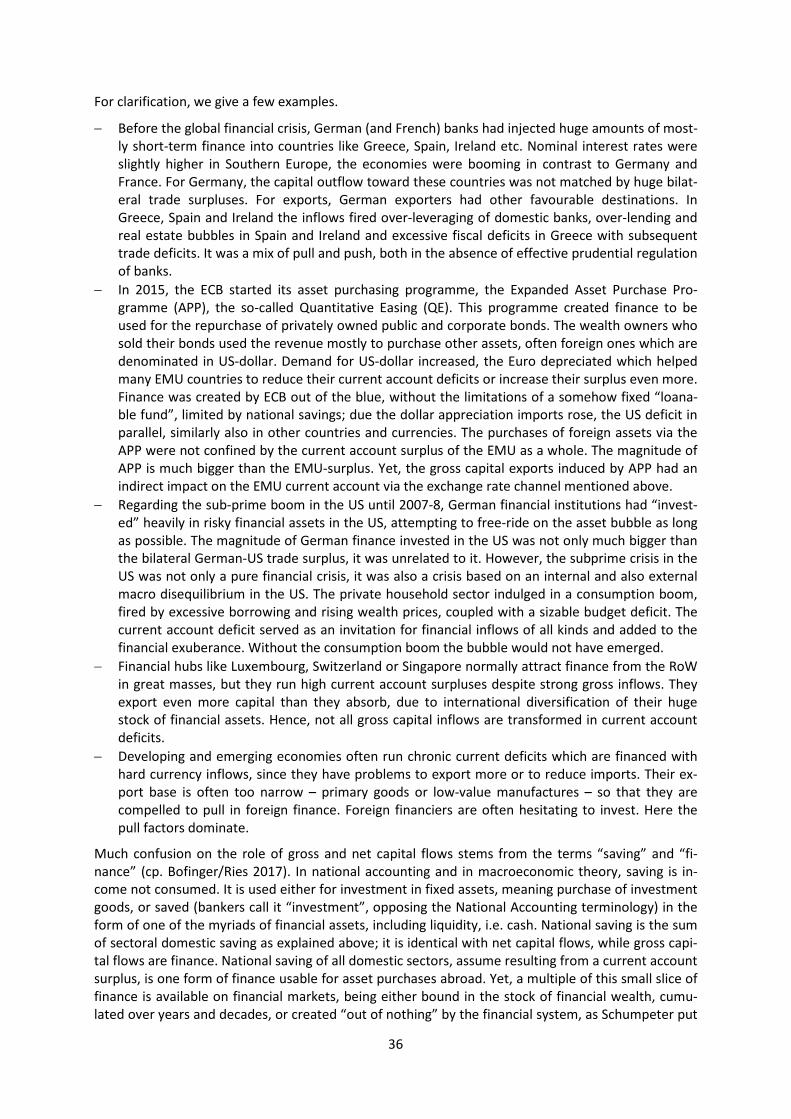
For clarification, we give a few examples.
− Before the global financial crisis, German (and French) banks had injected huge amounts of most-ly short-term finance into countries like Greece, Spain, Ireland etc. Nominal interest rates were slightly higher in Southern Europe, the economies were booming in contrast to Germany and France. For Germany, the capital outflow toward these countries was not matched by huge bilat-eral trade surpluses. For exports, German exporters had other favourable destinations. In Greece, Spain and Ireland the inflows fired over-leveraging of domestic banks, over-lending and real estate bubbles in Spain and Ireland and excessive fiscal deficits in Greece with subsequent trade deficits. It was a mix of pull and push, both in the absence of effective prudential regulation of banks.
− In 2015, the ECB started its asset purchasing programme, the Expanded Asset Purchase Pro-gramme (APP), the so-called Quantitative Easing (QE). This programme created finance to be used for the repurchase of privately owned public and corporate bonds. The wealth owners who sold their bonds used the revenue mostly to purchase other assets, often foreign ones which are denominated in US-dollar. Demand for US-dollar increased, the Euro depreciated which helped many EMU countries to reduce their current account deficits or increase their surplus even more. Finance was created by ECB out of the blue, without the limitations of a somehow fixed “loana-ble fund”, limited by national savings; due the dollar appreciation imports rose, the US deficit in parallel, similarly also in other countries and currencies. The purchases of foreign assets via the APP were not confined by the current account surplus of the EMU as a whole. The magnitude of APP is much bigger than the EMU-surplus. Yet, the gross capital exports induced by APP had an indirect impact on the EMU current account via the exchange rate channel mentioned above.
− Regarding the sub-prime boom in the US until 2007-8, German financial institutions had “invest-ed” heavily in risky financial assets in the US, attempting to free-ride on the asset bubble as long as possible. The magnitude of German finance invested in the US was not only much bigger than the bilateral German-US trade surplus, it was unrelated to it. However, the subprime crisis in the US was not only a pure financial crisis, it was also a crisis based on an internal and also external macro disequilibrium in the US. The private household sector indulged in a consumption boom, fired by excessive borrowing and rising wealth prices, coupled with a sizable budget deficit. The current account deficit served as an invitation for financial inflows of all kinds and added to the financial exuberance. Without the consumption boom the bubble would not have emerged.
− Financial hubs like Luxembourg, Switzerland or Singapore normally attract finance from the RoW in great masses, but they run high current account surpluses despite strong gross inflows. They export even more capital than they absorb, due to international diversification of their huge stock of financial assets. Hence, not all gross capital inflows are transformed in current account deficits.
− Developing and emerging economies often run chronic current deficits which are financed with hard currency inflows, since they have problems to export more or to reduce imports. Their ex-port base is often too narrow – primary goods or low-value manufactures – so that they are compelled to pull in foreign finance. Foreign financiers are often hesitating to invest. Here the pull factors dominate.
Much confusion on the role of gross and net capital flows stems from the terms “saving” and “fi-nance” (cp. Bofinger/Ries 2017). In national accounting and in macroeconomic theory, saving is in-come not consumed. It is used either for investment in fixed assets, meaning purchase of investment goods, or saved (bankers call it “investment”, opposing the National Accounting terminology) in the form of one of the myriads of financial assets, including liquidity, i.e. cash. National saving is the sum of sectoral domestic saving as explained above; it is identical with net capital flows, while gross capi-tal flows are finance. National saving of all domestic sectors, assume resulting from a current account surplus, is one form of finance usable for asset purchases abroad. Yet, a multiple of this small slice of finance is available on financial markets, being either bound in the stock of financial wealth, cumu-lated over years and decades, or created “out of nothing” by the financial system, as Schumpeter put
36
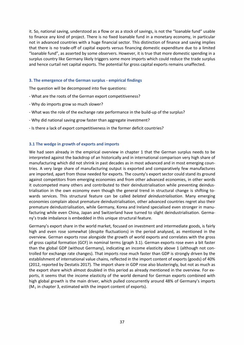
it. So, national saving, understood as a flow or as a stock of savings, is not the “loanable fund” usable to finance any kind of project. There is no fixed loanable fund in a monetary economy, in particular not in advanced countries with a huge financial sector. This distinction of finance and saving implies that there is no trade-off of capital exports versus financing domestic expenditure due to a limited “loanable fund”, as asserted by some observers. However, it is true that more domestic spending in a surplus country like Germany likely triggers some more imports which could reduce the trade surplus and hence curtail net capital exports. The potential for gross capital exports remains unaffected.
3. The emergence of the German surplus - empirical findings
The question will be decomposed into five questions:
- What are the roots of the German export competitiveness?
- Why do imports grow so much slower?
- What was the role of the exchange rate performance in the build-up of the surplus?
- Why did national saving grow faster than aggregate investment?
- Is there a lack of export competitiveness in the former deficit countries?
3.1 The wedge in growth of exports and imports
We had seen already in the empirical overview in chapter 1 that the German surplus needs to be interpreted against the backdrop of an historically and in international comparison very high share of manufacturing which did not shrink in past decades as in most advanced and in most emerging coun-tries. A very large share of manufacturing output is exported and comparatively few manufactures are imported, apart from those needed for exports. The county’s export sector could stand its ground against competitors from emerging economies and from other advanced economies, in other words it outcompeted many others and contributed to their deindustrialisation while preventing deindus-trialisation in the own economy even though the general trend in structural change is shifting to-wards services. This structural feature can be called belated deindustrialisation. Many emerging economies complain about premature deindustrialisation, other advanced countries regret also their premature deindustrialisation, while Germany, Korea and Ireland specialised even stronger in manu-facturing while even China, Japan and Switzerland have turned to slight deindustrialisation. Germa-ny’s trade imbalance is embedded in this unique structural feature.
Germany’s export share in the world market, focused on investment and intermediate goods, is fairly high and even rose somewhat (despite fluctuations) in the period analysed, as mentioned in the overview. German exports rose alongside the growth of world exports and correlates with the gross of gross capital formation (GCF) in nominal terms (graph 3.1). German exports rose even a bit faster than the global GDP (without Germany), indicating an income elasticity above 1 (although not con-trolled for exchange rate changes). That imports rose much faster than GDP is strongly driven by the establishment of international value chains, reflected in the import content of exports (goods) of 40% (2012, reported by Destatis 2017). The import share in GDP rose also blusteringly, but not as much as the export share which almost doubled in this period as already mentioned in the overview. For ex-ports, it seems that the income elasticity of the world demand for German exports combined with high global growth is the main driver, which pulled concurrently around 48% of Germany’s imports (M1 in chapter 3, estimated with the import content of exports).
37
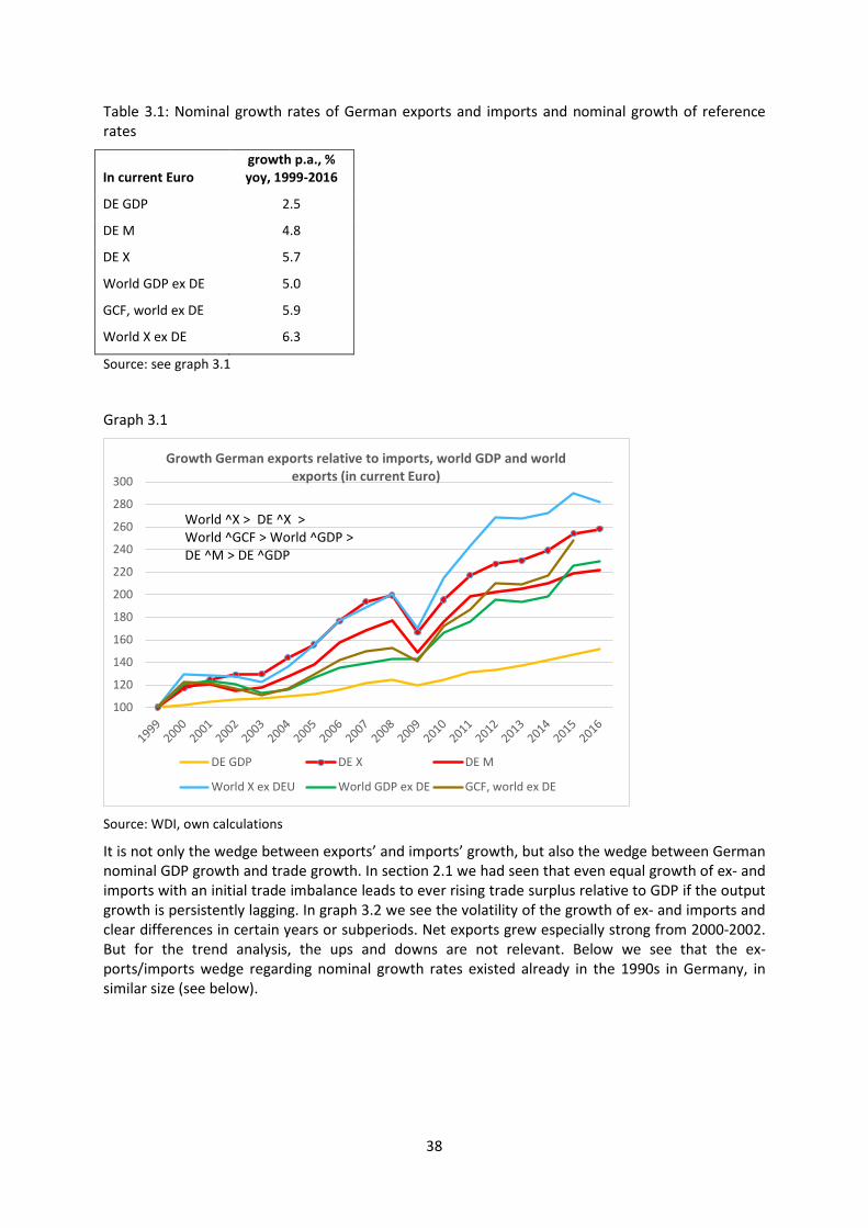
Table 3.1: Nominal growth rates of German exports and imports and nominal growth of reference rates
In current Euro growth p.a., % yoy, 1999-2016
DE GDP 2.5
DE M 4.8
DE X 5.7
World GDP ex DE 5.0
GCF, world ex DE 5.9
World X ex DE 6.3
Source: see graph 3.1
Graph 3.1
Source: WDI, own calculations
It is not only the wedge between exports’ and imports’ growth, but also the wedge between German nominal GDP growth and trade growth. In section 2.1 we had seen that even equal growth of ex- and imports with an initial trade imbalance leads to ever rising trade surplus relative to GDP if the output growth is persistently lagging. In graph 3.2 we see the volatility of the growth of ex- and imports and clear differences in certain years or subperiods. Net exports grew especially strong from 2000-2002. But for the trend analysis, the ups and downs are not relevant. Below we see that the ex-ports/imports wedge regarding nominal growth rates existed already in the 1990s in Germany, in similar size (see below).
100
120
140
160
180
200
220
240
260
280
300
Growth German exports relative to imports, world GDP and world exports (in current Euro)
DE GDP DE X DE M
World X ex DEU World GDP ex DE GCF, world ex DE
World ^X > DE ^X > World ^GCF > World ^GDP > DE ^M > DE ^GDP
38
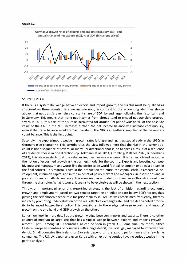
Graph 3.2
Source: AMECO
If there is a systematic wedge between export and import growth, the surplus must be qualified as structural on three counts. Here we assume now, in contrast to the accounting identities shown above, that net transfers remain a constant share of GDP, by and large, following the historical trend in Germany. This means that rising net incomes from abroad tend to exceed net transfers progres-sively. In 2016, this part of the surplus accounted for around 0.9 ppt of GDP or 9% of the absolute value of the CAS. If the NIIP increases further, the net income balance will increase continuously, even if the trade balance would remain constant. The NIB is a feedback amplifier of the current ac-count balance. This is the first point.
Secondly, the export/import wedge in growth rates is long-standing. It existed already in the 1990s in Germany (see chapter 4). This corroborates the view followed here that the rise in the current ac-count is not a sequence of several or many uni-directional shocks, so to speak a result of a sequence of accidental shocks in one direction (cp. Kollmann et al. 2014, Grömling/Matthes 2016, Bundesbank 2013); this view neglects that the rebalancing mechanisms are week. It is rather a trend rooted in the notion of export-led growth as the business model for the country. Exports and boosting compet-itiveness are mantras, magic words like the desire to be world football champion or at least a team in the final contest. This mantra is cast in the production structure, the capital stock, in research & de-velopment, in human capital and in the mindset of policy makers and managers, in institutions and in policies. It creates path dependency. It is even seen as a model for others, even though it would de-throne the champion. What is worse, it seems to be explosive as will be shown in the next section.
Thirdly, an important pillar of this export-led strategy is the lack of ambition regarding economic growth and employment, based on two tenets: targeting an inflation rate below ECB’s target, thus playing the self-chosen anchor role for price stability in EMU as was proclaimed frequently, thereby indirectly promoting undervaluation of the real effective exchange rate. and the deep-rooted procliv-ity to balanced budget fiscal policy. This contributes to the wedge between exports’ and imports’ growth on the one hand and GDP growth on the other.
Let us now look in more detail at the growth wedge between imports and exports. There is no other country of medium or large size that has a similar wedge between exports and imports growth – almost 1 ppt – among OECD countries, as can be seen in graph 3.3. Some small countries, either Eastern European countries or countries with a huge deficit, like Portugal, managed to improve their deficit. Small countries like Ireland or Slovenia depend on the export performance of a few large companies. The US, UK, Japan and even Korea with an extreme surplus have no serious wedge in the period analysed.
-2
-1
0
1
2
3
-20
-10
0
10
20
30
Germany: growth rates of exports and imports (incl. services), and annual change of net exports (NX), % of GDP (in current prices)
exports of goods and services, growth imports of goods and services, growth
change of NX, % of GDP (rhs)
39

Graph 3.3
Source: AMECO
Is the period 1999-2016 exceptional or is there a longer trend? In the table below we see that the wedge between exports and imports growth was even slightly bigger 1991-1999 than in the period 1999-2016, however, growth was around 1 ppt higher in the 1990s. The slower rise of the trade bal-ance in the 1990s was due to the lower base effect in the initial year 1991 and the by higher GDP growth in the 1990s, partly caused by more expansionary fiscal policy to cope with the challenges of the reunification of the country.
Table 3.2
Growth of nominal exports and imports (incl. services), GDP and the trade balance in Germany 1991-2016
Growth of nominal …, % p.a. 1991-1999 1999-2016 1991-2016
exports 5.08 5.74 5.64
Imports 3.97 4.78 4.65
GDP 3.56 2.48 2.62
Trade balance, % of GDP -1.7 (1991) 0.7 (1999) 7.6 (2016)
AMECO, own calculations
Whether and to what extent the wedge of the growth rates was driven by promoting price competi-tiveness and real undervaluation of the currency will be discussed in the next section.
3.2 Can exchange rates rebalance current accounts?
Here we analyse first the role of price competitiveness and the variety of indicators for it. Thereby we discuss the relationship between price- and non-price competitiveness. We also discuss the mostly neglected effects of exchange rate changes on domestic demand. In the second part we analyse the capacity of exchange rates to contribute to rebalance current account imbalances.
-3 -2 -1 0 1 2 3
PortugalGreece
LithuaniaLatvia
SloveniaSpain
GERMANYSlovakiaEstonia
MaltaAustria
NetherlandsIreland
ItalyUnited States
United KingdomLuxembourg
BelgiumKorea
CyprusSweden
JapanFrance
Finlandaverage EA
Exports' minus imports' growth rate p.a. in selected countries (goods and services, current prices, local currency), ranked, 1999-
2016, ppts
40
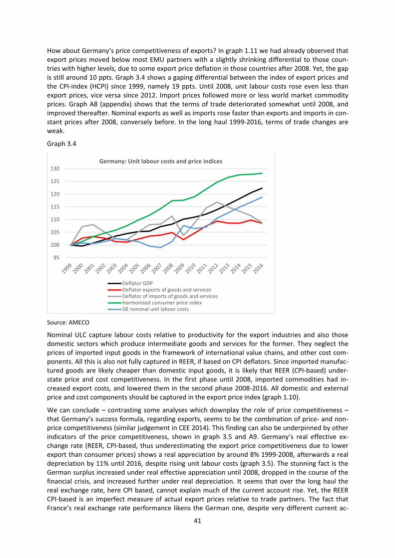
How about Germany’s price competitiveness of exports? In graph 1.11 we had already observed that export prices moved below most EMU partners with a slightly shrinking differential to those coun-tries with higher levels, due to some export price deflation in those countries after 2008. Yet, the gap is still around 10 ppts. Graph 3.4 shows a gaping differential between the index of export prices and the CPI-index (HCPI) since 1999, namely 19 ppts. Until 2008, unit labour costs rose even less than export prices, vice versa since 2012. Import prices followed more or less world market commodity prices. Graph A8 (appendix) shows that the terms of trade deteriorated somewhat until 2008, and improved thereafter. Nominal exports as well as imports rose faster than exports and imports in con-stant prices after 2008, conversely before. In the long haul 1999-2016, terms of trade changes are weak.
Graph 3.4
Source: AMECO
Nominal ULC capture labour costs relative to productivity for the export industries and also those domestic sectors which produce intermediate goods and services for the former. They neglect the prices of imported input goods in the framework of international value chains, and other cost com-ponents. All this is also not fully captured in REER, if based on CPI deflators. Since imported manufac-tured goods are likely cheaper than domestic input goods, it is likely that REER (CPI-based) under-state price and cost competitiveness. In the first phase until 2008, imported commodities had in-creased export costs, and lowered them in the second phase 2008-2016. All domestic and external price and cost components should be captured in the export price index (graph 1.10).
We can conclude – contrasting some analyses which downplay the role of price competitiveness – that Germany’s success formula, regarding exports, seems to be the combination of price- and non-price competitiveness (similar judgement in CEE 2014). This finding can also be underpinned by other indicators of the price competitiveness, shown in graph 3.5 and A9. Germany’s real effective ex-change rate (REER, CPI-based, thus underestimating the export price competitiveness due to lower export than consumer prices) shows a real appreciation by around 8% 1999-2008, afterwards a real depreciation by 11% until 2016, despite rising unit labour costs (graph 3.5). The stunning fact is the German surplus increased under real effective appreciation until 2008, dropped in the course of the financial crisis, and increased further under real depreciation. It seems that over the long haul the real exchange rate, here CPI based, cannot explain much of the current account rise. Yet, the REER CPI-based is an imperfect measure of actual export prices relative to trade partners. The fact that France’s real exchange rate performance likens the German one, despite very different current ac-
95
100
105
110
115
120
125
130Germany: Unit labour costs and price indices
Deflator GDPDeflator exports of goods and servicesDeflator of imports of goods and servicesHarmonised consumer price indexDE nominal unit labour costs
41
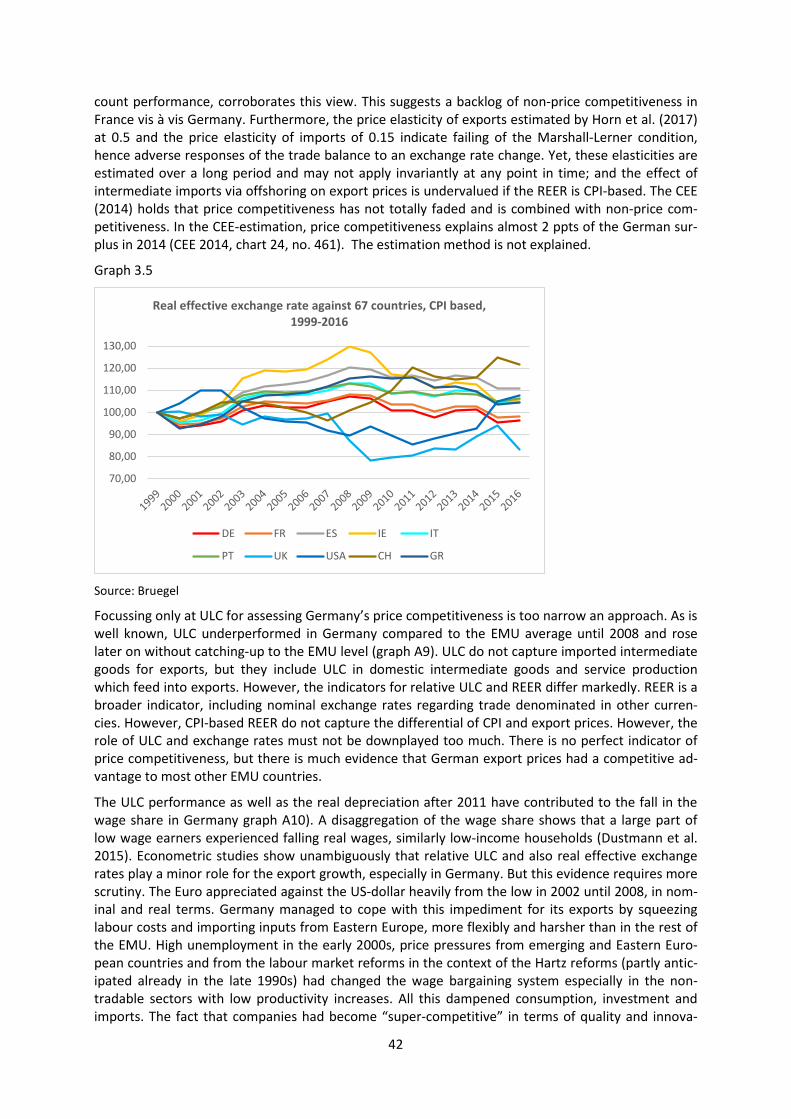
count performance, corroborates this view. This suggests a backlog of non-price competitiveness in France vis à vis Germany. Furthermore, the price elasticity of exports estimated by Horn et al. (2017) at 0.5 and the price elasticity of imports of 0.15 indicate failing of the Marshall-Lerner condition, hence adverse responses of the trade balance to an exchange rate change. Yet, these elasticities are estimated over a long period and may not apply invariantly at any point in time; and the effect of intermediate imports via offshoring on export prices is undervalued if the REER is CPI-based. The CEE (2014) holds that price competitiveness has not totally faded and is combined with non-price com-petitiveness. In the CEE-estimation, price competitiveness explains almost 2 ppts of the German sur-plus in 2014 (CEE 2014, chart 24, no. 461). The estimation method is not explained.
Graph 3.5
Source: Bruegel
Focussing only at ULC for assessing Germany’s price competitiveness is too narrow an approach. As is well known, ULC underperformed in Germany compared to the EMU average until 2008 and rose later on without catching-up to the EMU level (graph A9). ULC do not capture imported intermediate goods for exports, but they include ULC in domestic intermediate goods and service production which feed into exports. However, the indicators for relative ULC and REER differ markedly. REER is a broader indicator, including nominal exchange rates regarding trade denominated in other curren-cies. However, CPI-based REER do not capture the differential of CPI and export prices. However, the role of ULC and exchange rates must not be downplayed too much. There is no perfect indicator of price competitiveness, but there is much evidence that German export prices had a competitive ad-vantage to most other EMU countries.
The ULC performance as well as the real depreciation after 2011 have contributed to the fall in the wage share in Germany graph A10). A disaggregation of the wage share shows that a large part of low wage earners experienced falling real wages, similarly low-income households (Dustmann et al. 2015). Econometric studies show unambiguously that relative ULC and also real effective exchange rates play a minor role for the export growth, especially in Germany. But this evidence requires more scrutiny. The Euro appreciated against the US-dollar heavily from the low in 2002 until 2008, in nom-inal and real terms. Germany managed to cope with this impediment for its exports by squeezing labour costs and importing inputs from Eastern Europe, more flexibly and harsher than in the rest of the EMU. High unemployment in the early 2000s, price pressures from emerging and Eastern Euro-pean countries and from the labour market reforms in the context of the Hartz reforms (partly antic-ipated already in the late 1990s) had changed the wage bargaining system especially in the non-tradable sectors with low productivity increases. All this dampened consumption, investment and imports. The fact that companies had become “super-competitive” in terms of quality and innova-
70,00
80,00
90,00
100,00
110,00
120,00
130,00
Real effective exchange rate against 67 countries, CPI based, 1999-2016
DE FR ES IE IT
PT UK USA CH GR
42
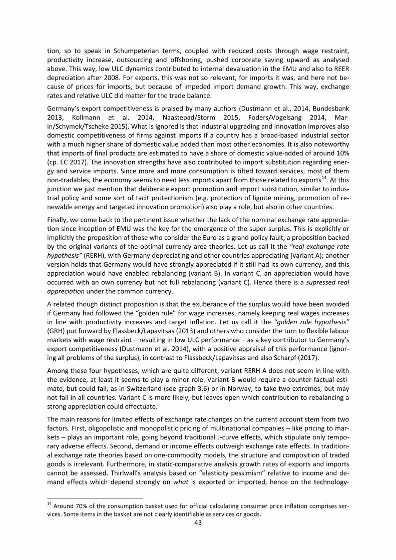
tion, so to speak in Schumpeterian terms, coupled with reduced costs through wage restraint, productivity increase, outsourcing and offshoring, pushed corporate saving upward as analysed above. This way, low ULC dynamics contributed to internal devaluation in the EMU and also to REER depreciation after 2008. For exports, this was not so relevant, for imports it was, and here not be-cause of prices for imports, but because of impeded import demand growth. This way, exchange rates and relative ULC did matter for the trade balance.
Germany’s export competitiveness is praised by many authors (Dustmann et al., 2014, Bundesbank 2013, Kollmann et al. 2014, Naastepad/Storm 2015, Foders/Vogelsang 2014, Mar-in/Schymek/Tscheke 2015). What is ignored is that industrial upgrading and innovation improves also domestic competitiveness of firms against imports if a country has a broad-based industrial sector with a much higher share of domestic value added than most other economies. It is also noteworthy that imports of final products are estimated to have a share of domestic value-added of around 10% (cp. EC 2017). The innovation strengths have also contributed to import substitution regarding ener-gy and service imports. Since more and more consumption is tilted toward services, most of them non-tradables, the economy seems to need less imports apart from those related to exports14. At this junction we just mention that deliberate export promotion and import substitution, similar to indus-trial policy and some sort of tacit protectionism (e.g. protection of lignite mining, promotion of re-newable energy and targeted innovation promotion) also play a role, but also in other countries.
Finally, we come back to the pertinent issue whether the lack of the nominal exchange rate apprecia-tion since inception of EMU was the key for the emergence of the super-surplus. This is explicitly or implicitly the proposition of those who consider the Euro as a grand policy fault, a proposition backed by the original variants of the optimal currency area theories. Let us call it the “real exchange rate hypothesis” (RERH), with Germany depreciating and other countries appreciating (variant A); another version holds that Germany would have strongly appreciated if it still had its own currency, and this appreciation would have enabled rebalancing (variant B). In variant C, an appreciation would have occurred with an own currency but not full rebalancing (variant C). Hence there is a supressed real appreciation under the common currency.
A related though distinct proposition is that the exuberance of the surplus would have been avoided if Germany had followed the “golden rule” for wage increases, namely keeping real wages increases in line with productivity increases and target inflation. Let us call it the “golden rule hypothesis” (GRH) put forward by Flassbeck/Lapavitsas (2013) and others who consider the turn to flexible labour markets with wage restraint – resulting in low ULC performance – as a key contributor to Germany’s export competitiveness (Dustmann et al. 2014), with a positive appraisal of this performance (ignor-ing all problems of the surplus), in contrast to Flassbeck/Lapavitsas and also Scharpf (2017).
Among these four hypotheses, which are quite different, variant RERH A does not seem in line with the evidence, at least it seems to play a minor role. Variant B would require a counter-factual esti-mate, but could fail, as in Switzerland (see graph 3.6) or in Norway, to take two extremes, but may not fail in all countries. Variant C is more likely, but leaves open which contribution to rebalancing a strong appreciation could effectuate.
The main reasons for limited effects of exchange rate changes on the current account stem from two factors. First, oligopolistic and monopolistic pricing of multinational companies – like pricing to mar-kets – plays an important role, going beyond traditional J-curve effects, which stipulate only tempo-rary adverse effects. Second, demand or income effects outweigh exchange rate effects. In tradition-al exchange rate theories based on one-commodity models, the structure and composition of traded goods is irrelevant. Furthermore, in static-comparative analysis growth rates of exports and imports cannot be assessed. Thirlwall’s analysis based on “elasticity pessimism” relative to income and de-mand effects which depend strongly on what is exported or imported, hence on the technology-
14 Around 70% of the consumption basket used for official calculating consumer price inflation comprises ser-vices. Some items in the basket are not clearly identifiable as services or goods.
43
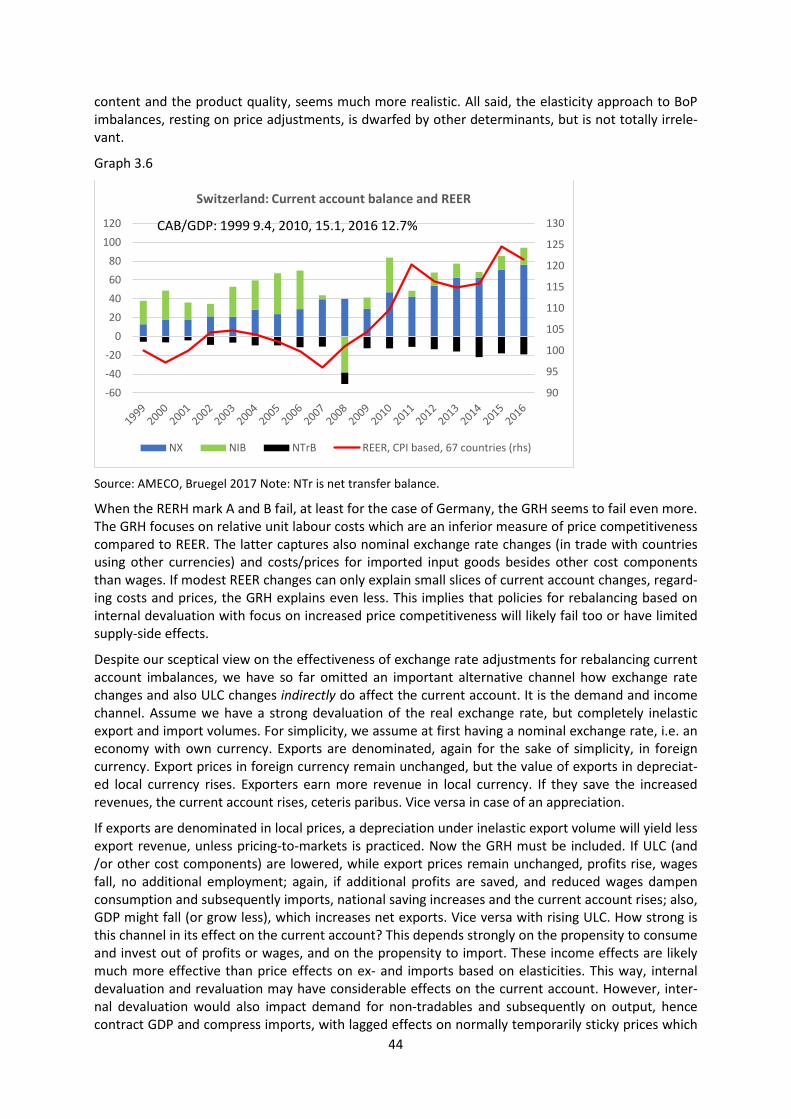
content and the product quality, seems much more realistic. All said, the elasticity approach to BoP imbalances, resting on price adjustments, is dwarfed by other determinants, but is not totally irrele-vant.
Graph 3.6
Source: AMECO, Bruegel 2017 Note: NTr is net transfer balance.
When the RERH mark A and B fail, at least for the case of Germany, the GRH seems to fail even more. The GRH focuses on relative unit labour costs which are an inferior measure of price competitiveness compared to REER. The latter captures also nominal exchange rate changes (in trade with countries using other currencies) and costs/prices for imported input goods besides other cost components than wages. If modest REER changes can only explain small slices of current account changes, regard-ing costs and prices, the GRH explains even less. This implies that policies for rebalancing based on internal devaluation with focus on increased price competitiveness will likely fail too or have limited supply-side effects.
Despite our sceptical view on the effectiveness of exchange rate adjustments for rebalancing current account imbalances, we have so far omitted an important alternative channel how exchange rate changes and also ULC changes indirectly do affect the current account. It is the demand and income channel. Assume we have a strong devaluation of the real exchange rate, but completely inelastic export and import volumes. For simplicity, we assume at first having a nominal exchange rate, i.e. an economy with own currency. Exports are denominated, again for the sake of simplicity, in foreign currency. Export prices in foreign currency remain unchanged, but the value of exports in depreciat-ed local currency rises. Exporters earn more revenue in local currency. If they save the increased revenues, the current account rises, ceteris paribus. Vice versa in case of an appreciation.
If exports are denominated in local prices, a depreciation under inelastic export volume will yield less export revenue, unless pricing-to-markets is practiced. Now the GRH must be included. If ULC (and /or other cost components) are lowered, while export prices remain unchanged, profits rise, wages fall, no additional employment; again, if additional profits are saved, and reduced wages dampen consumption and subsequently imports, national saving increases and the current account rises; also, GDP might fall (or grow less), which increases net exports. Vice versa with rising ULC. How strong is this channel in its effect on the current account? This depends strongly on the propensity to consume and invest out of profits or wages, and on the propensity to import. These income effects are likely much more effective than price effects on ex- and imports based on elasticities. This way, internal devaluation and revaluation may have considerable effects on the current account. However, inter-nal devaluation would also impact demand for non-tradables and subsequently on output, hence contract GDP and compress imports, with lagged effects on normally temporarily sticky prices which
90
95
100
105
110
115
120
125
130
-60-40-20
020406080
100120
Switzerland: Current account balance and REER
NX NIB NTrB REER, CPI based, 67 countries (rhs)
CAB/GDP: 1999 9.4, 2010, 15.1, 2016 12.7%
44
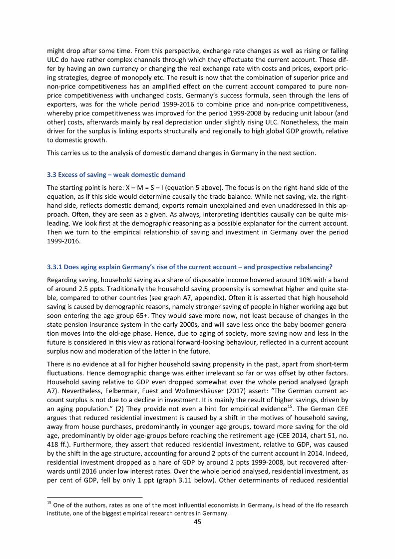
might drop after some time. From this perspective, exchange rate changes as well as rising or falling ULC do have rather complex channels through which they effectuate the current account. These dif-fer by having an own currency or changing the real exchange rate with costs and prices, export pric-ing strategies, degree of monopoly etc. The result is now that the combination of superior price and non-price competitiveness has an amplified effect on the current account compared to pure non-price competitiveness with unchanged costs. Germany’s success formula, seen through the lens of exporters, was for the whole period 1999-2016 to combine price and non-price competitiveness, whereby price competitiveness was improved for the period 1999-2008 by reducing unit labour (and other) costs, afterwards mainly by real depreciation under slightly rising ULC. Nonetheless, the main driver for the surplus is linking exports structurally and regionally to high global GDP growth, relative to domestic growth.
This carries us to the analysis of domestic demand changes in Germany in the next section.
3.3 Excess of saving – weak domestic demand
The starting point is here: X – M = S – I (equation 5 above). The focus is on the right-hand side of the equation, as if this side would determine causally the trade balance. While net saving, viz. the right-hand side, reflects domestic demand, exports remain unexplained and even unaddressed in this ap-proach. Often, they are seen as a given. As always, interpreting identities causally can be quite mis-leading. We look first at the demographic reasoning as a possible explanator for the current account. Then we turn to the empirical relationship of saving and investment in Germany over the period 1999-2016.
3.3.1 Does aging explain Germany’s rise of the current account – and prospective rebalancing?
Regarding saving, household saving as a share of disposable income hovered around 10% with a band of around 2.5 ppts. Traditionally the household saving propensity is somewhat higher and quite sta-ble, compared to other countries (see graph A7, appendix). Often it is asserted that high household saving is caused by demographic reasons, namely stronger saving of people in higher working age but soon entering the age group 65+. They would save more now, not least because of changes in the state pension insurance system in the early 2000s, and will save less once the baby boomer genera-tion moves into the old-age phase. Hence, due to aging of society, more saving now and less in the future is considered in this view as rational forward-looking behaviour, reflected in a current account surplus now and moderation of the latter in the future.
There is no evidence at all for higher household saving propensity in the past, apart from short-term fluctuations. Hence demographic change was either irrelevant so far or was offset by other factors. Household saving relative to GDP even dropped somewhat over the whole period analysed (graph A7). Nevertheless, Felbermair, Fuest and Wollmershäuser (2017) assert: “The German current ac-count surplus is not due to a decline in investment. It is mainly the result of higher savings, driven by an aging population.” (2) They provide not even a hint for empirical evidence15. The German CEE argues that reduced residential investment is caused by a shift in the motives of household saving, away from house purchases, predominantly in younger age groups, toward more saving for the old age, predominantly by older age-groups before reaching the retirement age (CEE 2014, chart 51, no. 418 ff.). Furthermore, they assert that reduced residential investment, relative to GDP, was caused by the shift in the age structure, accounting for around 2 ppts of the current account in 2014. Indeed, residential investment dropped as a hare of GDP by around 2 ppts 1999-2008, but recovered after-wards until 2016 under low interest rates. Over the whole period analysed, residential investment, as per cent of GDP, fell by only 1 ppt (graph 3.11 below). Other determinants of reduced residential
15 One of the authors, rates as one of the most influential economists in Germany, is head of the ifo research institute, one of the biggest empirical research centres in Germany.
45
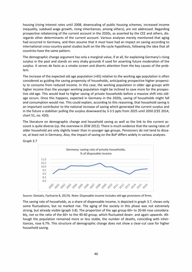
housing (rising interest rates until 2008, downscaling of public housing schemes, increased income inequality, subdued wage growth, rising inheritances, among others), are not addressed. Regarding prospective rebalancing of the current account in the 2020s, as asserted by the CEE and others, dis-regards other determinants of the current account. Various analyses merely mentioned that aging had occurred in Germany, and then assume that it must have had an impact on saving according to international cross-country-panel studies built on the life-cycle hypothesis, following the idea that all countries have the same pattern.
The demographic change argument has only a marginal value, if at all, for explaining Germany’s rising surplus in the past and stands on very shaky grounds if used for asserting future moderation of the surplus. It serves de facto as a smoke screen and diverts attention from the key causes of the prob-lem.
The increase of the expected old age population (+65) relative to the working age population is often considered as guiding the saving propensity of households, anticipating prospective higher propensi-ty to consume from reduced income. In this case, the working population in older age groups with higher income than the younger working population might be inclined to save more for the prospec-tive old-age. This would lead to higher saving of private households before a massive shift into old-age occurs. Once this happens, expected in Germany in the 2020s, saving of households might fall and consumption would rise. This could explain, according to this reasoning, that household saving is an important contributor to the national increase of saving which generated the current surplus and in the future a stabiliser pulling the surplus downward by 3-3.5 ppts from 2025 until 2050 (CEE 2014, chart 51, no. 420).
The literature on demographic change and household saving as well as the link to the current ac-count is quite diverse (cp. the overview in ZEW 2012). There is much evidence that the saving rates of older household are only slightly lower than in younger age groups. Pensioners do not tend to dissa-ve, at least not in Germany. Also, the impact of saving on the BoP differs widely in various analyses.
Graph 3.7
Source: Destatis, Fachserie 8, 2017b. Note: Disposable income includes old-age provisions of firms.
The saving rate of households, as a share of dispensable income, is depicted in graph 3.7, shows only some fluctuations, but no marked rise. The aging of the society in this phase was not extremely strong, but already visible (graph 3.8). The proportion of the age group 60+ to 20-60 rose considera-bly, not so the ratio of the 60+ to the 40-60 group, which fluctuated down- and again upwards. Alt-hough the population remained more or less stable, the number of deaths, coinciding with inher-itances, rose 6.7%. This structure of demographic change does not show a clear-cut case for higher household saving.
8,0 8,5 9,0 9,5
10,0 10,5 11,0
Germany: saving rate of private households, % of disposable income
46

Graph 3.8
Source: Destatis 2017b, own calculations.
For the prospects until 2030, the transition to old age will accelerate strongly (graph 3.9). The popu-lation will shrink slightly (following the 13th population projection published by Destatis), while the ratio of +65 to the 40-60 group is forecast to rise from 58% to 81% and the number of deaths by 10%. Indeed, it sounds plausible that the rising share of pensioners will likely have a reduced propensity to save, while the presumed group of strong savers, the 40-60 group, declines by 10% in the period 2015-30.
Graph 3.9
Source: Destatis 2015, own calculations
Forecasting saving rates has to consider diverse motives and should be done with caution. More im-portant is, however, that the increasing old-age population is likely correlating with less residential investment. Further, if pensioners’ incomes are reduced, it is likely that consumption falls somewhat too which would impede investment and also imports of consumption goods. Shrinking populations normally leads to lower GDP growth and less imports, in Germany especially after 2030. Overall, the balance of reduced saving and reduced investment may not have a strong impact on the current account. Deutsche Bundesbank emphasised the opposing trends of higher old-age consumption pro-pensity and less housing investment (2012, 56), with regard to the current account.
Even if aging would have led in the past and until the early 2020s to more household saving after controlling for residential investment, an effect on the current account would only occur if it happens to a stronger extent than in countries that are trade partners.
02004006008001000
40
60
80
100
Germany 1999-2016: demographic changes
60+/20-60%, % 60+/40-60, %
population, mn deaths (1000s), rhs
850
900
950
1000
1050
30405060708090
Germany: aging society 2015-2030
population, mn ratio 65+/20-65, %ratio 65+/40-65%, % deaths, 1000s, rhs
47
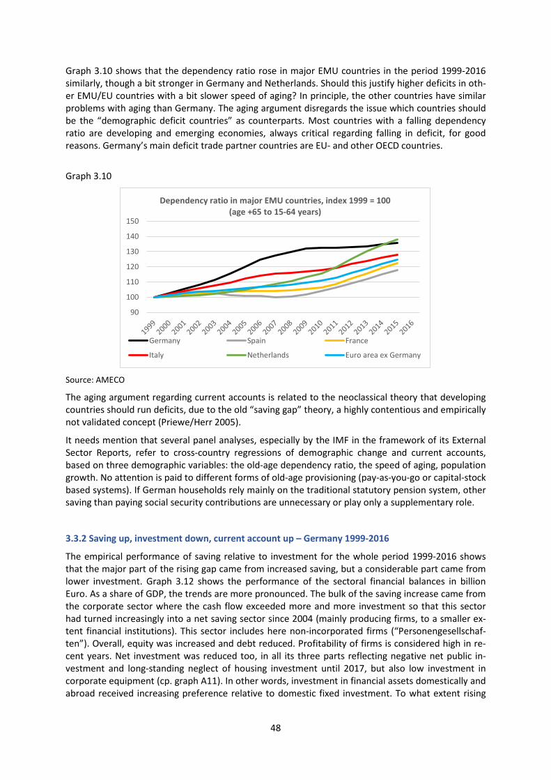
Graph 3.10 shows that the dependency ratio rose in major EMU countries in the period 1999-2016 similarly, though a bit stronger in Germany and Netherlands. Should this justify higher deficits in oth-er EMU/EU countries with a bit slower speed of aging? In principle, the other countries have similar problems with aging than Germany. The aging argument disregards the issue which countries should be the “demographic deficit countries” as counterparts. Most countries with a falling dependency ratio are developing and emerging economies, always critical regarding falling in deficit, for good reasons. Germany’s main deficit trade partner countries are EU- and other OECD countries.
Graph 3.10
Source: AMECO
The aging argument regarding current accounts is related to the neoclassical theory that developing countries should run deficits, due to the old “saving gap” theory, a highly contentious and empirically not validated concept (Priewe/Herr 2005).
It needs mention that several panel analyses, especially by the IMF in the framework of its External Sector Reports, refer to cross-country regressions of demographic change and current accounts, based on three demographic variables: the old-age dependency ratio, the speed of aging, population growth. No attention is paid to different forms of old-age provisioning (pay-as-you-go or capital-stock based systems). If German households rely mainly on the traditional statutory pension system, other saving than paying social security contributions are unnecessary or play only a supplementary role.
3.3.2 Saving up, investment down, current account up – Germany 1999-2016
The empirical performance of saving relative to investment for the whole period 1999-2016 shows that the major part of the rising gap came from increased saving, but a considerable part came from lower investment. Graph 3.12 shows the performance of the sectoral financial balances in billion Euro. As a share of GDP, the trends are more pronounced. The bulk of the saving increase came from the corporate sector where the cash flow exceeded more and more investment so that this sector had turned increasingly into a net saving sector since 2004 (mainly producing firms, to a smaller ex-tent financial institutions). This sector includes here non-incorporated firms (“Personengesellschaf-ten”). Overall, equity was increased and debt reduced. Profitability of firms is considered high in re-cent years. Net investment was reduced too, in all its three parts reflecting negative net public in-vestment and long-standing neglect of housing investment until 2017, but also low investment in corporate equipment (cp. graph A11). In other words, investment in financial assets domestically and abroad received increasing preference relative to domestic fixed investment. To what extent rising
90
100
110
120
130
140
150
Dependency ratio in major EMU countries, index 1999 = 100 (age +65 to 15-64 years)
Germany Spain France
Italy Netherlands Euro area ex Germany
48
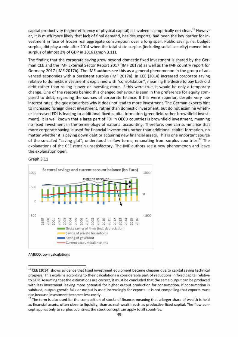
capital productivity (higher efficiency of physical capital) is involved is empirically not clear.16 Howev-er, it is much more likely that lack of final demand, besides exports, had been the key barrier for in-vestment in face of frozen real aggregate consumption over a long spell. Public saving, i.e. budget surplus, did play a role after 2014 when the total state surplus (including social security) moved into surplus of almost 2% of GDP in 2016 (graph 3.11).
The finding that the corporate saving grew beyond domestic fixed investment is shared by the Ger-man CEE and the IMF External Sector Report 2017 (IMF 2017a) as well as the IMF country report for Germany 2017 (IMF 2017b). The IMF authors see this as a general phenomenon in the group of ad-vanced economies with a persistent surplus (IMF 2017a). In CEE (2014) increased corporate saving relative to domestic investment is explained with “consolidation”, meaning the desire to pay back old debt rather than rolling it over or investing more. If this were true, it would be only a temporary change. One of the reasons behind this changed behaviour is seen in the preference for equity com-pared to debt, regarding the sources of corporate finance. If this were superior, despite very low interest rates, the question arises why it does not lead to more investment. The German experts hint to increased foreign direct investment, rather than domestic investment, but do not examine wheth-er increased FDI is leading to additional fixed capital formation (greenfield rather brownfield invest-ment). It is well known that a large part of FDI in OECD countries is brownfield investment, meaning no fixed investment in the terminology of national accounting. Therefore, one can summarise that more corporate saving is used for financial investments rather than additional capital formation, no matter whether it is paying down debt or acquiring new financial assets. This is one important source of the so-called “saving glut”, understood in flow terms, emanating from surplus countries.17 The explanations of the CEE remain unsatisfactory. The IMF authors see a new phenomenon and leave the explanation open.
Graph 3.11
AMECO, own calculations
16 CEE (2014) shows evidence that fixed investment equipment became cheaper due to capital saving technical progress. This explains according to their calculations a considerable part of reductions in fixed capital relative to GDP. Assuming that the estimations are correct, it must be concluded that the same output can be produced with less investment leaving more potential for higher output production for consumption. If consumption is subdued, output growth falls or output is used increasingly for exports. It is not compelling that exports must rise because investment becomes less costly. 17 The term is also used for the composition of stocks of finance, meaning that a larger share of wealth is held as financial assets, often close to liquidity, than as real wealth such as productive fixed capital. The flow con-cept applies only to surplus countries, the stock concept can apply to all countries.
-1000
0
1000
-500
0
500
1000
1999
2000
2001
2002
2003
2004
2005
2006
2007
2008
2009
2010
2011
2012
2013
2014
2015
2016
Sectoral savings and current account balance (bn Euro)
Gross saving of firms (incl. depreciation)Saving of private householdsSaving of governmtCurrent account balance, rhs
current account
49
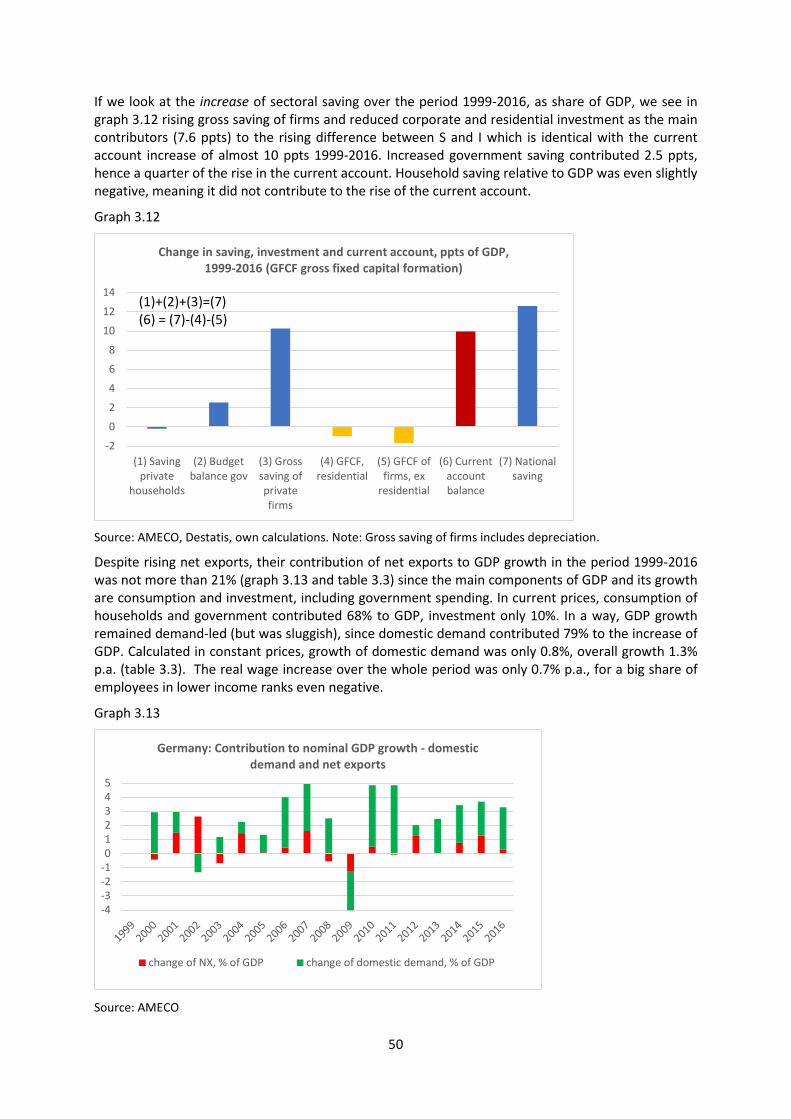
If we look at the increase of sectoral saving over the period 1999-2016, as share of GDP, we see in graph 3.12 rising gross saving of firms and reduced corporate and residential investment as the main contributors (7.6 ppts) to the rising difference between S and I which is identical with the current account increase of almost 10 ppts 1999-2016. Increased government saving contributed 2.5 ppts, hence a quarter of the rise in the current account. Household saving relative to GDP was even slightly negative, meaning it did not contribute to the rise of the current account.
Graph 3.12
Source: AMECO, Destatis, own calculations. Note: Gross saving of firms includes depreciation.
Despite rising net exports, their contribution of net exports to GDP growth in the period 1999-2016 was not more than 21% (graph 3.13 and table 3.3) since the main components of GDP and its growth are consumption and investment, including government spending. In current prices, consumption of households and government contributed 68% to GDP, investment only 10%. In a way, GDP growth remained demand-led (but was sluggish), since domestic demand contributed 79% to the increase of GDP. Calculated in constant prices, growth of domestic demand was only 0.8%, overall growth 1.3% p.a. (table 3.3). The real wage increase over the whole period was only 0.7% p.a., for a big share of employees in lower income ranks even negative.
Graph 3.13
Source: AMECO
-2
0
2
4
6
8
10
12
14
(1) Savingprivate
households
(2) Budgetbalance gov
(3) Grosssaving ofprivatefirms
(4) GFCF,residential
(5) GFCF offirms, ex
residential
(6) Currentaccountbalance
(7) Nationalsaving
Change in saving, investment and current account, ppts of GDP, 1999-2016 (GFCF gross fixed capital formation)
(1)+(2)+(3)=(7) (6) = (7)-(4)-(5)
-4-3-2-1012345
Germany: Contribution to nominal GDP growth - domestic demand and net exports
change of NX, % of GDP change of domestic demand, % of GDP
50
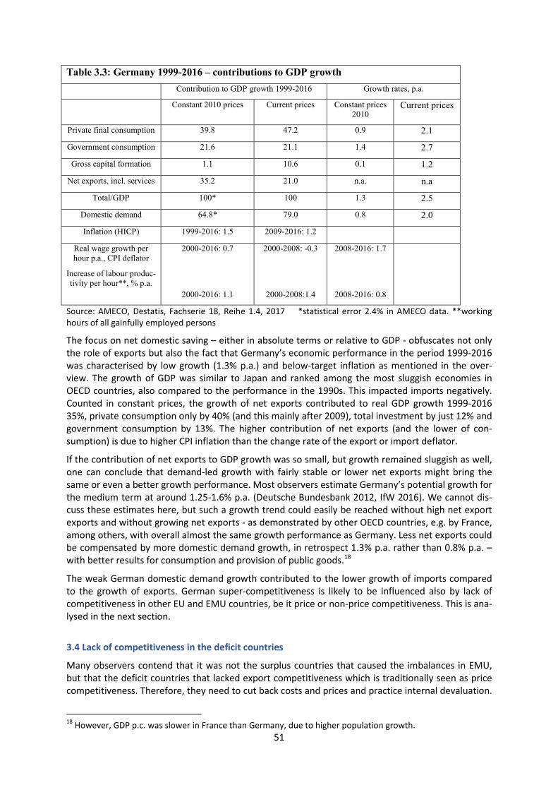
Table 3.3: Germany 1999-2016 – contributions to GDP growth
Contribution to GDP growth 1999-2016 Growth rates, p.a.
Constant 2010 prices Current prices Constant prices 2010
Current prices
Private final consumption 39.8 47.2 0.9 2.1
Government consumption 21.6 21.1 1.4 2.7
Gross capital formation 1.1 10.6 0.1 1.2
Net exports, incl. services 35.2 21.0 n.a. n.a
Total/GDP 100* 100 1.3 2.5
Domestic demand 64.8* 79.0 0.8 2.0
Inflation (HICP) 1999-2016: 1.5 2009-2016: 1.2
Real wage growth per hour p.a., CPI deflator
Increase of labour produc-tivity per hour**, % p.a.
2000-2016: 0.7
2000-2016: 1.1
2000-2008: -0.3
2000-2008:1.4
2008-2016: 1.7
2008-2016: 0.8
Source: AMECO, Destatis, Fachserie 18, Reihe 1.4, 2017 *statistical error 2.4% in AMECO data. **working hours of all gainfully employed persons
The focus on net domestic saving – either in absolute terms or relative to GDP - obfuscates not only the role of exports but also the fact that Germany’s economic performance in the period 1999-2016 was characterised by low growth (1.3% p.a.) and below-target inflation as mentioned in the over-view. The growth of GDP was similar to Japan and ranked among the most sluggish economies in OECD countries, also compared to the performance in the 1990s. This impacted imports negatively. Counted in constant prices, the growth of net exports contributed to real GDP growth 1999-2016 35%, private consumption only by 40% (and this mainly after 2009), total investment by just 12% and government consumption by 13%. The higher contribution of net exports (and the lower of con-sumption) is due to higher CPI inflation than the change rate of the export or import deflator.
If the contribution of net exports to GDP growth was so small, but growth remained sluggish as well, one can conclude that demand-led growth with fairly stable or lower net exports might bring the same or even a better growth performance. Most observers estimate Germany’s potential growth for the medium term at around 1.25-1.6% p.a. (Deutsche Bundesbank 2012, IfW 2016). We cannot dis-cuss these estimates here, but such a growth trend could easily be reached without high net export exports and without growing net exports - as demonstrated by other OECD countries, e.g. by France, among others, with overall almost the same growth performance as Germany. Less net exports could be compensated by more domestic demand growth, in retrospect 1.3% p.a. rather than 0.8% p.a. – with better results for consumption and provision of public goods.18
The weak German domestic demand growth contributed to the lower growth of imports compared to the growth of exports. German super-competitiveness is likely to be influenced also by lack of competitiveness in other EU and EMU countries, be it price or non-price competitiveness. This is ana-lysed in the next section.
3.4 Lack of competitiveness in the deficit countries
Many observers contend that it was not the surplus countries that caused the imbalances in EMU, but that the deficit countries that lacked export competitiveness which is traditionally seen as price competitiveness. Therefore, they need to cut back costs and prices and practice internal devaluation.
18 However, GDP p.c. was slower in France than Germany, due to higher population growth. 51
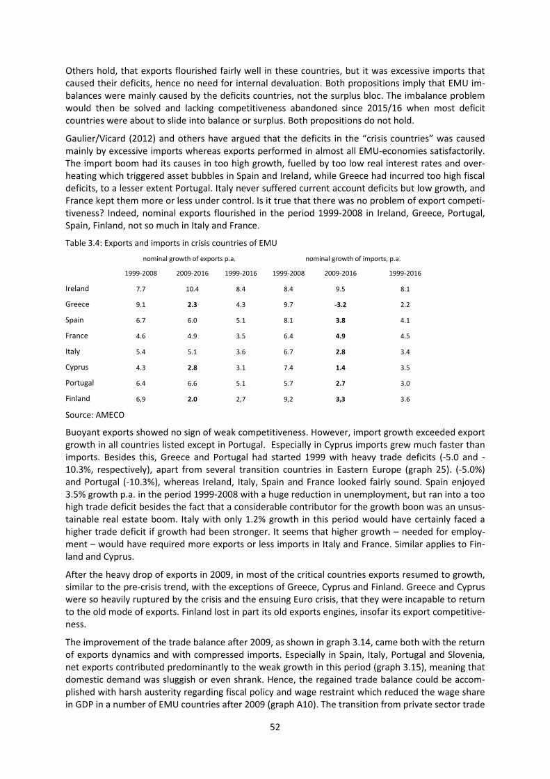
Others hold, that exports flourished fairly well in these countries, but it was excessive imports that caused their deficits, hence no need for internal devaluation. Both propositions imply that EMU im-balances were mainly caused by the deficits countries, not the surplus bloc. The imbalance problem would then be solved and lacking competitiveness abandoned since 2015/16 when most deficit countries were about to slide into balance or surplus. Both propositions do not hold.
Gaulier/Vicard (2012) and others have argued that the deficits in the “crisis countries” was caused mainly by excessive imports whereas exports performed in almost all EMU-economies satisfactorily. The import boom had its causes in too high growth, fuelled by too low real interest rates and over-heating which triggered asset bubbles in Spain and Ireland, while Greece had incurred too high fiscal deficits, to a lesser extent Portugal. Italy never suffered current account deficits but low growth, and France kept them more or less under control. Is it true that there was no problem of export competi-tiveness? Indeed, nominal exports flourished in the period 1999-2008 in Ireland, Greece, Portugal, Spain, Finland, not so much in Italy and France.
Table 3.4: Exports and imports in crisis countries of EMU
nominal growth of exports p.a. nominal growth of imports, p.a.
1999-2008 2009-2016 1999-2016 1999-2008 2009-2016 1999-2016
Ireland 7.7 10.4 8.4 8.4 9.5 8.1
Greece 9.1 2.3 4.3 9.7 -3.2 2.2
Spain 6.7 6.0 5.1 8.1 3.8 4.1
France 4.6 4.9 3.5 6.4 4.9 4.5
Italy 5.4 5.1 3.6 6.7 2.8 3.4
Cyprus 4.3 2.8 3.1 7.4 1.4 3.5
Portugal 6.4 6.6 5.1 5.7 2.7 3.0
Finland 6,9 2.0 2,7 9,2 3,3 3.6
Source: AMECO
Buoyant exports showed no sign of weak competitiveness. However, import growth exceeded export growth in all countries listed except in Portugal. Especially in Cyprus imports grew much faster than imports. Besides this, Greece and Portugal had started 1999 with heavy trade deficits (-5.0 and -10.3%, respectively), apart from several transition countries in Eastern Europe (graph 25). (-5.0%) and Portugal (-10.3%), whereas Ireland, Italy, Spain and France looked fairly sound. Spain enjoyed 3.5% growth p.a. in the period 1999-2008 with a huge reduction in unemployment, but ran into a too high trade deficit besides the fact that a considerable contributor for the growth boon was an unsus-tainable real estate boom. Italy with only 1.2% growth in this period would have certainly faced a higher trade deficit if growth had been stronger. It seems that higher growth – needed for employ-ment – would have required more exports or less imports in Italy and France. Similar applies to Fin-land and Cyprus.
After the heavy drop of exports in 2009, in most of the critical countries exports resumed to growth, similar to the pre-crisis trend, with the exceptions of Greece, Cyprus and Finland. Greece and Cyprus were so heavily ruptured by the crisis and the ensuing Euro crisis, that they were incapable to return to the old mode of exports. Finland lost in part its old exports engines, insofar its export competitive-ness.
The improvement of the trade balance after 2009, as shown in graph 3.14, came both with the return of exports dynamics and with compressed imports. Especially in Spain, Italy, Portugal and Slovenia, net exports contributed predominantly to the weak growth in this period (graph 3.15), meaning that domestic demand was sluggish or even shrank. Hence, the regained trade balance could be accom-plished with harsh austerity regarding fiscal policy and wage restraint which reduced the wage share in GDP in a number of EMU countries after 2009 (graph A10). The transition from private sector trade
52
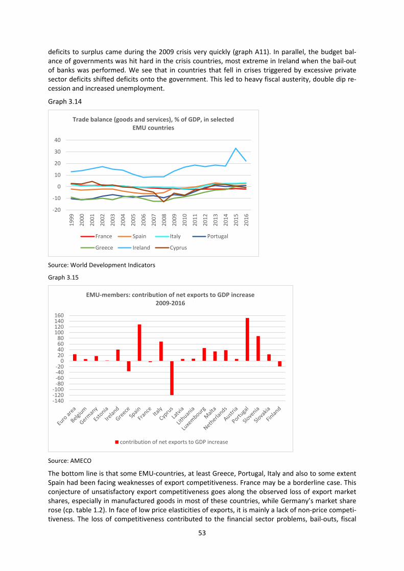
deficits to surplus came during the 2009 crisis very quickly (graph A11). In parallel, the budget bal-ance of governments was hit hard in the crisis countries, most extreme in Ireland when the bail-out of banks was performed. We see that in countries that fell in crises triggered by excessive private sector deficits shifted deficits onto the government. This led to heavy fiscal austerity, double dip re-cession and increased unemployment.
Graph 3.14
Source: World Development Indicators
Graph 3.15
Source: AMECO
The bottom line is that some EMU-countries, at least Greece, Portugal, Italy and also to some extent Spain had been facing weaknesses of export competitiveness. France may be a borderline case. This conjecture of unsatisfactory export competitiveness goes along the observed loss of export market shares, especially in manufactured goods in most of these countries, while Germany’s market share rose (cp. table 1.2). In face of low price elasticities of exports, it is mainly a lack of non-price competi-tiveness. The loss of competitiveness contributed to the financial sector problems, bail-outs, fiscal
-20
-10
0
10
20
30
40
1999
2000
2001
2002
2003
2004
2005
2006
2007
2008
2009
2010
2011
2012
2013
2014
2015
2016
Trade balance (goods and services), % of GDP, in selected EMU countries
France Spain Italy Portugal
Greece Ireland Cyprus
-140-120-100
-80-60-40-20
020406080
100120140160
EMU-members: contribution of net exports to GDP increase 2009-2016
contribution of net exports to GDP increase
53
problems and the remaining debt overhang. The exuberant austerity and pressure on wages aggra-vated the calamities greatly. If the competitiveness problem is misdiagnosed as lack of price and cost competitiveness, a downward deflationary spiral would be set in motion with low effectiveness on exports but strong effects on domestic demand and imports. If growth starts to normalise again after overcoming the backlog due to the financial crisis and the subsequent double dip crisis, it is likely that trade deficits will return if domestic demand picks up again.
The too strong rise of imports until 2008 was a result of pull and push. Some countries were willing to finance the deficits, mainly Germany and France. Financing trade deficits does not necessarily re-quire running a surplus. The excessive deficits of the peripheral countries would not have emerged if they were not heavily supported by other countries’ banking sectors.
All in all, even though the crisis countries seemed to enjoy flourishing exports in the period 1999-2008, high growth and continuous improvement of employment require in several countries better export competitiveness, mainly of the non-price type, such as in Greece, Italy, Cyprus, Portugal and also in France if the current accounts shall not return to deficits. Their price- and non-price competi-tiveness is squeezed by Germany and other surplus countries and low-cost countries in Eastern Eu-rope and Asia. The fact that Germany, Netherlands and a few other surplus countries have reached exorbitant surpluses until 2016 while the former deficit countries stay back reflects – besides de-mand weaknesses – also lack of export competitiveness, compared to the EMU champions. The weakness of export demand reflects also the compressed imports. The latter are to some extent the exports of other peripheral countries.
3.5 Summing up – Germany’s “super competitiveness”
Germany’s “super-competitiveness” means that the country has a high and seemingly continuously rising current account surplus, deeply embedded in the structure of the economy. The latter evolved historically over many decades, but changed towards a chronic surplus not before the inception of the EMU. The trend to ever rising surplus emerged already in the 1980s – the peak current account was reached 1988 with 4.5% of GDP, the trade balance peaked 1990 with 5.5% – but was averted by the huge wave of increased domestic demand in the course of the German re-unification in the 1990s, including a massive construction boom (cp. Graph A2). The real effective appreciation of the DM from 1989 until 1995 by 19% (REER CPI-based, against 67 trading partners, Bruegel 2018) con-tributed to reducing the surplus. If such a tsunami of revived domestic demand is unlikely to be repli-cated by whatever political efforts one can imagine, a high “structural surplus” seems unavoidable, at least in the medium term. This is based on the emergence of a huge manufacturing sector, as a share of value added in GDP, withstanding worldwide trends towards deindustrialisation and a rising ser-vice sector. Germany’s manufacturing sector, the production base of its exports of which a great part is exported, is a unique feature comparable only to Korea (among larger advanced economies), whereas Japan and Switzerland have started reducing their manufacturing value added, relative to GDP. This structural or supply-side part of the German surplus which tends to increase due to the long-standing wedge in growth rates of exports and imports is hard to quantify, relative to the de-mand-side part.
The benefits from the rise of the surplus for the German economy, in terms of growth and increases in consumption, are markedly small. Increased competitiveness in the sense used in this study means that Germany increased its share in world exports at the expense of other countries. Yet, countries like France with almost balanced current account achieved similar growth rates in the period ana-lysed. Germany’s growth performance over the whole period, but especially in the first part until 2008, was poor. The much-praised emergence of the German economy from Europe’s “sick man” (The Economist) to Europe’s “superstar” (Dustmann et al. 2015) is not backed by many indicators, such as investment, consumption, poverty and income distribution, old-age provisioning, housing shortage, etc.
54
The wedge between growth rates of exports and imports can be explained predominantly by the high global income elasticity of exports, higher growth of world demand than domestic aggregate de-mand, increasing import content of exports due to outsourcing and offshoring, and subdued domes-tic final demand. The latter is caused by wage moderation, fiscal restraint, subdued private sector investment, including residential investment, and excessive corporate saving. The super-competitiveness led to a triple surplus of the private households, the corporate sector and the gov-ernment sector; such a constellation is unique in international comparison.
Changes of the real exchange rate played a minor role in their effect on the volumes of traded goods. Yet, relative unit labour costs and real devaluation after 2008 favoured profit performance and dampened domestic demand. The channels how real exchange rates as well as relative ULC effectu-ate exports and imports are more complex than most analyses assert. The demand channel seems to be much more important than the supply channel via costs and prices. Despite the low price elastici-ty of exports and imports, which do not suffice the Marshall-Lerner condition, the exchange rate is extremely important for the emergence of the German surplus: it is very likely that without the common currency, Germany would have appreciated its domestic currency massively, such as Swit-zerland or oil exporters in periods of oil price booms under flexible exchange rate regimes. This does not mean that exchange rate changes would have balanced the current accounts; a scenario like in Switzerland cannot be excluded. However, gauging a counterfactual development involves much uncertainty. Nevertheless, the IMF, the Peterson Institute for International Economics (Cline 2017)19 and indirectly also the German CEE hold that Germany’s real exchange rate is heavily undervalued.
The puzzle of slow imports dynamics, apart from imports earmarked for exports as intermediate goods, is easy to decipher. The low import content of final consumption and to a lesser extent of domestic investment has four main roots: (i) sluggish domestic demand growth, (ii) superior competi-tiveness of domestic production vis à vis imports (the twin-effect of export competitiveness), (iii) structural change of domestic final demand toward services which are predominantly not tradable, and (iv) import substitution regarding energy and commodity imports. De facto mercantilist policies for export promotion and import substitution in manifold ways – tax laws and regulations, direct and indirect subsidies, applied research and development, targeted infrastructure, training and educa-tion, direct political support for export marketing – played also a role. De facto it is something that is named in other countries “industrial policy”.
Demographic change towards aging of the society played so far no identifiable role. This diagnosis would change somewhat if slowed-down residential construction (until recently) were caused verifi-ably by demographic change, as asserted by the German CEE (2014). Even then it would explain only a small part of the surplus.
The German surplus was spurred by the generation of overly high current account deficits in the pe-ripheral EMU countries, caused by asset bubbles in real estate markets or by too high fiscal deficits as in Greece and to a lesser extent in Portugal. These deficits were fired by gross capital exports – main-ly excessive bank lending – to these countries, predominantly by German and French financial institu-tions; the consequence of gross capital exports had been, combined with domestic over-leveraging, rising trade deficits. However, it is noteworthy mentioning that the geographic structure of bilateral trade balances does not coincide with the geographic structure of gross or net bilateral capital ex-ports. Germany had only a small slice of its trade surplus vis à vis the periphery countries, since its surplus is concentrated on the US, UK, France and Austria, but injected huge amounts of finance into the “crisis countries”. France did the same, but encountered no trade surplus (cp. Chen et al. 2012).
Even though a large part of the explanation of the deficits in the peripheral countries until 2008 stem from excessive imports, there are presumably in a number of countries severe deficiencies of export
19 This is implicated in Cline (2017) who looks only at EMU as an aggregate. But the limits for all countries are set at +/-3% of GDP. It is assumed that “fundamental real exchange rates” will lead to current accounts in this band.
55
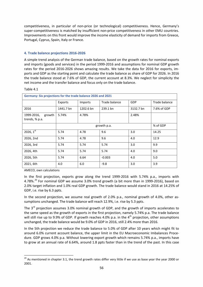
competitiveness, in particular of non-price (or technological) competitiveness. Hence, Germany’s super-competitiveness is matched by insufficient non-price competitiveness in other EMU countries. Improvements on this front would improve the income elasticity of demand for imports from Greece, Portugal, Cyprus, Spain, Italy or France.
4. Trade balance projections 2016-2026
A simple trend analysis of the German trade balance, based on the growth rates for nominal exports and imports (goods and services) in the period 1999-2016 and assumptions for nominal GDP growth rates for the period 2016-2026 shows amazing results. We take the data for 2016 for exports, im-ports and GDP as the starting point and calculate the trade balance as share of GDP for 2026. In 2016 the trade balance stood at 7.6% of GDP, the current account at 8.3%. We neglect for simplicity the net income and the transfer balance and focus only on the trade balance.
Table 4.1
Germany: Six projections for the trade balance 2026 and 2021
Exports Imports Trade balance GDP Trade balance
2016 1441.7 bn 1202.6 bn 239.1 bn 3132.7 bn 7.6% of GDP
1999-2016, growth trends, % p.a.
5.74% 4.78% 2.48%
growth p.a. % of GDP
2026, 1st 5.74 4.78 9.6 3.0 14.25
2026, 2nd 5.74 4.78 9.6 4.0 12.9
2026, 3rd 5.74 5.74 5.74 3.0 9.9
2026, 4th 5.74 5.74 5.74 4.0 9.0
2026, 5th 5.74 6.64 -0.003 4.0 5.0
2021, 6th 4.0 6.0 -9.8 3.0 3.9
AMECO, own calculations
In the first projection, exports grow along the trend 1999-2016 with 5.74% p.a., imports with 4.78%.20 For nominal GDP we assume 3.0% trend growth (a bit more than in 1999-2016), based on 2.0% target inflation and 1.0% real GDP growth. The trade balance would stand in 2016 at 14.25% of GDP, i.e. rise by 6.3 ppts.
In the second projection, we assume real growth of 2.0% p.a., nominal growth of 4.0%, other as-sumptions unchanged. The trade balance will reach 12.9%, i.e. rise by 5.3 ppts.
The 3rd projection assumes 3.0% nominal growth of GDP, and the growth of imports accelerates to the same speed as the growth of exports in the first projection, namely 5.74% p.a. The trade balance will still rise up to 9.9% of GDP. If growth reaches 4.0% p.a. in the 4th projection, other assumptions unchanged, the trade balance would be 9.0% of GDP in 2016, still 2.4% more than 2016.
In the 5th projection we reduce the trade balance to 5.0% of GDP after 10 years which might fit to around 6.0% current account balance, the upper limit in the EU Macroeconomic Imbalances Proce-dure. GDP grows 4.0% p.a. Without lowering export growth which remains 5.74% p.a., imports have to grow at an annual rate of 6.64%, around 1.8 ppts faster than in the trend of the past. In this case
20 As mentioned in chapter 3.1, the trend growth rates differ very little if we use as base year the year 2000 or 2001.
56
the imports-GDP-ratio rises from 38% to 49% of GDP, and the marginal increase of imports, as a share of the GDP increase, would rise from 64% to 80%.
In the 6th projection over only 5 years until 2021, the trade balance will drop to 3.9% of GDP, which might be close to a current account of 5%. Growth of exports decelerates to only 4.0% p.a., and im-ports rise by 6.0%, while nominal GDP trends with 3.0%. Net exports contribute negatively to GDP growth. The trade balance shrinks strongly in absolute terms.
The almost explosive growth of the trade balance in the first four projections has – among other fac-tors – to do with the base effect. Once exports are initially much higher than imports, exponential growth of exports and imports makes the trade balance grow much faster. In the case of linear growth, the trade balance would rise too, but much slower. Since German exports are correlated with global growth, which has grown boisterously in the past, the assumption of exponential growth is as justified as for the much slower GDP growth trend for Germany, the key driver for its imports.
The unfavourable base effect of 2016 with the high trade imbalance constitutes an accelerating and hazardous factor.
Note that projections are not forecasts. Reality does not always follow trends. Forward looking ra-tional expectations, functioning as self-fulfilling prophecies, might be at work – but all too often not or too late and at high social costs. If there is no clear and stable current account equilibrium, neither country-specific nor generic, then there are is a multitude of short-term equilibria, some of which may be advantageous, others less, some disastrous. Policy rules have to chip in. This is also the logic of IMF’s “External Balance Assessment” (EBA, see IMF 2017) which calls for multilateral action.
Potential stabilising mechanisms
Aren’t there any stabilising or rectifying factors at work? Candidates are real effective exchange rate changes, less growth in importing countries due to BoP constrained growth or other impediments, higher imports from countries delivering intermediate goods for German exports, more imports due to rapid aging in Germany, supply constraints in Germany due to labour shortage, lower growth in OECD or in emerging economies, or new emerging competitors. All these factors are ambiguous in their effects on the trade and current account balance:
− High GDP growth: Germany might return to stronger dynamics of domestic demand pushed by rising wages, due to selective labour supply bottlenecks, which however can be overcome by re-ducing unemployment, increasing the participation rate of the labour force, especially by trans-forming involuntary part-time into full-time work and by immigration. This would be limited to the medium term and might induce rising labour productivity. Imports would rise, but exports too.
− Labour shortage in Germany may limit growth of exports, but also growth of GDP and hence of imports. Growth rates of both ex- and imports would fall with an ambiguous result. Yet, also productivity increases could pick up again. Labour shortage could also be attenuated by reducing part-time work, raising wages and attract immigration. This would impact both ex- and imports.
− Exchange rates: The Euro might rise against the US-dollar and other currencies. This would im-pede growth in other EMU countries and also in Germany, which dampens the growth of imports too. The direct effect of a real appreciation of the Euro on German exports is small due to the low price elasticity (apart from adverse effects), but the indirect effect on profits and aggregate saving is more important.
− BoP-constrained growth: An increasing trade and current account surplus will likely curb both intra and extra EU imbalances. This will indeed push other countries into deficits again and on a reduced growth trend. Again, the negative effects on German exports will dampen Germany’s growth and its imports with an ambiguous overall effect on the trade balance.
57
− Eastern Europe: More imports from Eastern Europe and emerging economies: This seems to be already the trend of the past whose mirror image is growth in Eastern Europe which conversely fuels German exports.
− Aging population: It is true that the propensity to save might drop in private households, thus reducing aggregate saving. But counter-effects have to be heeded: strong decline of the popula-tion (absent strong immigration) with normally lower growth, in particular via less residential in-vestment and less consumption. The aging argument will likely materialise not before the mid-2020s when big cohorts of elderly retire. Residential investment is held to be reduced by shrink-ing age groups below 40 in which the home purchase is a dominant saving motive. It is more like-ly that house construction picks up due to continued low interest rates. If the latter rise, house construction might fall and increase the current account.
− Lower growth in OECD and emerging countries: This is indeed likely to happen, including lower growth in the flagship of emerging economies, China. Again, growth of German exports may fal-ter, but growth of imports too.
− New competitors: This may occur, but Germany’s standing in its segment of investment goods, based on long-standing human capital accumulation, is hard to contest severely. It may not be excluded that China is successful in technological upgrading and competes more intensively with segments in which German producers are strong.
It looks as if there is no realistic stabiliser in sight. In most cases mentioned exports might grow slow-er, dampening export-led growth and subsequently imports. Once a rising surplus was not prevent-ed, path dependency is at work. We have not yet addressed opportunities to raise domestic demand and excluded policy measures. It seems that market forces are not capable to induce rebalancing, at least not in a currency union with the institutional setting of the EMU.
In contrast to the potentially stabilising factors, there might be drivers for even higher surpluses. Much depends on further growth of emerging economies. Especially those in Latin America are faced presently with severe problems or deep recessions like Brazil. If they return to growth, Germany will befit. If the US implement corporate tax reductions which spur growth, given strong rise of deficits and debt, the US trade deficit might rise offering more opportunities for strong European exporters. If Iran, Libya, Venezuela and Russia overcome their specific problems, German exports are attracted, and oil prices might fall again. Finally, if EMU countries from the periphery make good their backlog after almost 10 years of lost GDP compared to the level of 2008, domestic demand in these countries will pick up, including investment. If countries slide again in deficits, German net exports would go booming.
The German debates about “digitalisation of production” have led the “Platform Industry 4.0”, allud-ing to the 4th industrial revolution (http://www.plattform-i40.de/I40/Navigation/DE/Home/home.html). This initiative is a collaboration of two Federal Minis-tries and industrial associations and can be considered as classical corporatist industrial policy. If it gave German manufacturing a further boost toward high technology and even higher competitive-ness against other countries, the surplus would certainly rise. This is not unlikely since there is a grand consensus among political parties and civil society to embark on this neo-mercantilist road. It seems indeed that promoting exports is a “holy cow” in Germany, as remarked by Richard Cooper (2017, 186).
Even if the current account surplus could be stabilised at a certain high level, perhaps similar to Ko-rea, the question remains whether extreme export dependence is beneficial for the economy and its trade partners. Specifically, this question stands in the context of the EMU. These issues will be dis-cussed in chapter 8.
However, if the German surplus, combined with other EMU surplus countries, would move into the double digits, severe political headwind is likely to generate massive tensions, within EMU and in the global arena.
58
5. “International competitiveness” – a dangerous obsession?
In most analyses of the European imbalances the term “international competitiveness” (IC) is used but not defined. It can have many different meanings. Using the term for the microeconomic analysis of firms, or of a sector, it can make sense. Many use it with the aim of increasing a firm’s market share on the global market. Since not every firm can become champion, it would be a prescription for ever heading on toward “number one” like in the football premier league. Others hold that profitably selling goods internationally is the meaning of IC. Some analysts call for the “ability to sell” which should be improved in order get a competitive lead or catching-up against competitors. Such defini-tions may have their merits for corporate strategies, but can this work for nations or for all exports of a country, such as national “export competitiveness”?
The macroeconomic interpretation of IC looks like a mere aggregation exercise. Increased “export competitiveness”, as it is often called, would mean a rising world market share for a country or avoid-ing a reduction or maintaining the stance. It looks limited to exports. Yet, all exports of one country are other countries’ imports. At times, the IC is used as pertaining only to “price competitiveness”, measured by relative unit labour costs or by the real effective exchange rate. Non-price or technolog-ical competitiveness is neglected. The latter is sometimes also summarised as “structural” competi-tiveness”. These terms are not clearly defined on the macro level, based on sound economic theory.
Assume IC means improving the price and non-price competitiveness of the exports of a nation, aim-ing at a higher market share in the world market – as if the country were a corporation. In a simple 2-country-world model, country G would raise its market share against country F which represents all foreign countries. Globally, all exports are equal to all imports. Since country G’s exports are country F’s imports, G would export more but import less from F – if other factors that might impact the trade balance do not change. G has now a surplus, F runs a deficit (assume in the outset trade was balanced). IC would mean creating trade imbalances and striving to increase them more and more. If F is not so successful as G, it should fight harder. The aim for all countries should be to chase G, and G would chase the others. If this concept of competing for better IC were accepted and actively pur-sued by the governments of G and F, it would be a revival of ancient and crude mercantilism – it is not about pursuing the “comparative advantage” following David Ricardo and many of his followers for free trade, but the goal would be to accomplish a trade surplus, and every increase in the world market share would compellingly increase the surplus and the deficit of F as the mirror image. Using the microeconomic concept of IC as a macroeconomic one runs into a fallacy of aggregation that perverts free trade into mercantilism.
Of course, our example is static. The main adjustments in case of a trade imbalance, as shown be-tween G and F, are as follows: (i) a higher export share of G could trigger higher output growth of G which absorbs more imports; (ii) G’s currency might appreciate (in real terms) against F’s currency so that G exports less and imports more. (iii) F might be compelled to dampen growth which leads to less imports from G. (iv) F catches up with G by improving its export competitiveness. In all four cases the increased export share of G would be reversed, either in full or to a certain extent. Rebalancing would follow suit. Thus, trade imbalances would remain small and be subject to swift re-stabilisation. G’s gain in competitiveness would be limited and only temporary, a short-term issue we should not fuss about. However, the meaning of promoting national IC is normally not constrained to the short run. It is – implicitly or explicitly – considered a strategic issue with a persistent increase of the mar-ket share. Now the mercantilist flavour chips in.
But isn’t mercantilism the protectionist activity of the State, promoting exports and impeding im-ports? Yes, it is. But a country’s striving to become and remain champion or being as close as possible to championship leads automatically to less imports. Furthermore, modern production, be it for do-mestic demand or for exports, requires more education, skills, infrastructure, hence public goods than ever before. The more dependent a country is on its exports, the more it has to take care of “export competitiveness” – but not necessarily by subsidies or import tariffs or outright non-tariff measures. Innovation policy and other policies have similar or even stronger effects. “Standortpoli-
59
tik” (policies for locational improvement) is the new mantra. This black-box-term can be filled with content at will. It can be the guarantee of low corporate taxes as in Ireland, in order to attract multi-nationals, or becoming a financial hub as in Luxembourg or Cyprus, or with semi-industrial policy favouring, say, the car industry, chemical industry or engineering, renewal energy policy for replacing fossil imports, survival support for dirty lignite mining to conserve employment, imposing favourable trade rules and regulations on others, etc.
Country G striving like a corporation for a competitive advantage which lead to a higher market share, and hence an increase of its surplus, raises – by implication – net capital exports. It buys more debt certificates or similar foreign assets from F than it sells to F. This is the mirror image of less im-ports. G purchases less goods from F, but more of F’s assets thus impairing F’s net international in-vestment position. Now we have distorted “trade”: G specialises in selling goods, F specialises more and more in selling financial papers. This is not what Ricardo and all the followers considered free trade. And it is not sustainable.
All said, promoting IC of nations leads likely to trade and current account imbalances because not every country can be equally successful. No problem if imbalances are temporary and rebalancing comes soon. Temporary moderate imbalances would then be a sign of vivid competition. IC as a mac-roeconomic goal for all is therefore an ambiguous idea. It can be a dangerous obsession, as Krugman (1994) noted long ago, because it undermines the old idea of the usefulness of free trade for both partners involved. It implies however – mostly unintentionally, but not always – a mercantilist bias.
The upshot of our reasoning is that avoiding the fallacy of aggregation and the risks of trade imbal-ances requires that multilateral rules for trade and prudent current account balance have to be es-tablished, especially in a currency union without the option of nominal exchange rate adjustments.
This does not mean that the term “competitiveness” should be banned. We use it here in the sense of increasing a nation’s market share in the world market. This term should be framed by an interna-tional order for preventing and correcting BoP-imbalances. If markets do not find stable equilibria for the current account, normative goals should be used and implemented by rules and policies. Red lines for “excessive” surplus or deficit should be used, as intended in the regulatory framework of the IMF with its “External Balance Assessment” (EBA, IMF 2017) or with the European “Macroeconomic Imbalance Procedure” (MIP, EC 2016) or as envisaged by Cline/Williamson (2012) from the Peterson Institute for International Economics with their +/-3% band goal for the current account of all coun-tries. Although the regulatory frameworks proposed by the IMF and the MIP have – in our opinion – severe flaws and shortcomings, they share the same well justified goal. In such a framework, coun-tries with “excessive” deficits should improve their “competitiveness”, and those with excessive sur-plus should seek for corrective policies. This can be seen as a kind of prudent international “Ord-nungspolitik” (a kind of firm regulatory or legal framework for the functioning of markets), as coined by the German so-called ordo-liberals from the Freiburg School of economics.
6. Why is the German surplus a problem?
Many observers, mainly in Germany, do not see a problem – or not a grave one – with the German surplus. Others hold that the ensuing problems are so severe that the functioning of the monetary union is at risk and for the survival of EMU as a whole. In the latter case imbalances would be an Achilles heel for the EMU. Many other economists and policy makers stand between the two poles. The predominant view among policymakers of all political parties and leading economists in Germany is still that running a surplus is good, a sign of success, and has no negative repercussions. This is also the official opinion of the Ministry of Finance and the Ministry of the Economy in the German Federal Government. There is no radar system that is sensitive for the problem.
We proceed in this section as follows. First, we discuss disadvantages for the surplus country, here Germany. Second, we turn to disadvantages for the peripheral EMU countries, until 2012/2013 the deficit countries, afterwards swinging toward surplus too.
60
6.1 Potential problems for Germany
So far, Germany has not gained much – in macroeconomic terms – from its rising surplus since 1999. Average GDP growth was low in the period 1999-2016, not more than France that followed a domes-tic demand-led growth pattern, and conspicuously less than in the UK or in the US as chronic deficit countries. Obviously, a surplus in the current account can be in line with high growth, as in China from 2000 until 2007 or in Korea since long, or in line with low growth as in Japan after the financial crisis in 1990.
In Germany, private consumption as well as residential investment grew very slowly, less than GDP, similarly gross capital formation of corporations. The functional and personal Income distribution became more unequal. The net international investment position improved strongly, as a share of GDP, but with large claims on the ECB (TARGET2 balances) which are not remunerated. Overall, the return on assets remained puny. After 2009, growth and employment picked up, especially after the Euro crisis was overcome in 2014, but this seems to be a cyclical upswing, driven now mainly by do-mestic demand and some favourable external conditions. The country is highly dependent on the ups and downs of world markets, driven strongly by China, the US, UK and several large EMU partners. Net exports are dependent on countries running current account deficits and their sustainability. There is no doubt that further rise of the German surplus, following the trends of exports’ and im-ports’ growth paths, is not sustainable. Insofar as the surplus was partly driven by below-target-inflation, as set by the ECB, facilitated by low increase of ULC, relative to the EMU-partners, and low prices for imports, it fuelled deflationary risks in EMU. This occurred not only due to Germany’s too low inflation, but also by pushing countries first into deficits (or exploiting their pull traction incon-siderately) and then into “internal devaluation” with deflationary pressure on wages and prices. This in turn contributed to ECB’s zero interest rate policy and unconventional asset purchase pro-grammes. Monetary policy of the ECB de facto boosted fiscal policy in Germany (and elsewhere) by reducing interest payments on public debt, thus compensating somewhat otherwise restrictive fiscal policy.
Germany’s macroeconomic performance over the period 1999-2016 is overall dismal despite im-provements after 2009. Raising the surplus goes along with compressing growth of consumption (and also residential investment), the final goal of GDP growth and investment. There is little general ben-efit from being an “export superstar”, apart from the export sector. Maximising savings alongside the current account surplus has generated not much return, but many risks. This does not imply that a demand-led growth strategy leads necessarily and always to higher potential output growth. But output would be produced for the country, giving more weight to consumption and public goods, and it would avoid pushing EMU- and other countries into either intra-EMU deficits or external sur-plus against the RoW.
Should Germany pursue a higher growth path, say close to 2%, driven by rising domestic demand and more employment as well as increasing productivity, then a high but – by and large – stable surplus, relative to GDP, could be benevolent for the country. However, risks for deficit countries and for the functioning of the Euro system would remain. If the surplus allows to increase potential growth, ei-ther until full employment is reached or by inducing stronger technical progress precipitated in stronger growth of labour productivity, also more imports might be induced. This way the country would likely not increase its global market shares in exports, since other countries are offered more export opportunities. In this respect, China’s rising surplus in 2000-2008 differed markedly from Germany’s. Once a country has built up a capital stock, both fixed and human capital, geared pre-dominantly for exports, everything has to be subordinated to the supremacy of “export competitive-ness” and “globalisation”. This counts for policies, employment, wages, R&D, taxes and regulations – “Standortpolitik” or “locational policies”, a weasel word that circumscribes mercantilism in disguise as mentioned above. Of course, open protectionism would be inappropriate for an export-led econ-omy. Albeit, there are plenty and much better suitable substitutes for import tariffs and normal non-tariff barriers. Weal and woe of the economy depend on exports. Since they are volatile and highly sensitive to shocks, a flexible labour market – or significant parts of it – is imperative.
61

The two sub-periods 1999-2008 and 2009-2016 differ markedly in several aspects. In the second phase the German economy performed on standard macro indicators much better, as if the first woeful phase would pay off belatedly. This is true insofar as in the first phase price and non-price competitiveness including global value chains for intermediate input goods had been established with a clear lead vis à vis most other competitors from inside and outside EMU. This rendered possi-ble another leap in the trade surplus, now against extra EU nations, mainly the US and the UK. Yet, what is more important is (i) the unconventional monetary policy of the ECB, alleviating the debt burden including the debt overhang on banks and sovereigns in former crisis countries, (ii) the under-valuation of the Euro against the US-Dollar and the dollar-bloc, including China, (iii) reduced com-modity prices for imports, and (iv) the fall in unemployment with emerging bottlenecks in some seg-ments of the labour market, conditional on unusually low productivity growth. The super-surplus in the current account, heading for a further spike despite resuscitated domestic demand, seems out of control, heralding unsustainability and risks.
Summing up in the next box, the main downsides of the German surplus for the German economy had been the following – reflecting a multitude of mainly macroeconomic distortions.
Box 6.1: Germany’s burden with its high surplus
− Constrained growth of domestic demand and of fixed capital formation; exports growth has partly re-placed growth of consumption
− Requirement of a high dose of labour market flexibility for adjusting to the volatilities of export markets and exchange rates, thus undermining the traditional model of moderately centralised collective bargain-ing and the welfare state; dualizing the labour market with a large segment of flexible working poor em-ployment
− Increased regional disparities since export industries are often clustered in certain regions, while other regions are drained and etiolated
− Disappointing financial investments abroad, especially with blind bubble investment
− Pressure for below-target inflation and price as well as corporate tax competitiveness to support non-price competitiveness; thus, inducing deflation risks in slumps and recessions; pushing deficit countries into in-ternal devaluation which reinforces deflationary risks in the aftermath of bubbles
− Misfit of the Euro-US-Dollar exchange rate (and other exchange rates), as they neither fit the deficit- nor the surplus countries, or the super- and the small-surplus countries alike
− Misfit of the ECB’s monetary policy as it is not appropriate for the surplus and the deficit countries even-handedly
− Pushing the EMU into overall surplus against the RoW, pushing them into either protectionism or devalua-tion
− Financial risks if surpluses are financed mainly short-term, by portfolio equity or short-term debt, with risks of sudden withdrawals, maturity mismatch and rollover risks for debtors
Among the problems listed in Box 6.1, the most hazardous one is likely the deflation risk. This is vo-cally emphasised by the External Sector Report of the IMF (2017, 27, recurring on Eichengreen/Temin 2010, Blanchard/Milesi-Feretti 2011 and Caballero et al. 2016):
“A historical example – that should serve as warning also for policymakers today – is the in-terwar gold standard of the 1920s and early 1930s. Insufficient adjustment of surplus coun-tries (at the time including the United States and France) complicated efforts of deficit coun-tries (including the United Kingdom and Germany) with large debt burdens and paved the way for the Great Depression. Lack of exchange rate flexibility and contractionary policies by surplus countries – implemented inter alia to constrain inflation and preserve competitive positions – contributed to the rigidity of external positions, features that have parallels in to-day’s constellation […]. Excess global saving also pushes down the equilibrium level of inter-
62
est rates. If interest rates get near their effective lower bounds, this can push countries into liquidity traps., thus triggering declines in output and higher unemployment […]”
This note applies especially to the EMU which has resemblance to the interwar Gold Standard with no opportunity for nominal appreciation. Today, Germany has taken over the place of the US and France at the time.
Surpluses may be sustained and moderated with less downsides if
− based on high growth in the surplus country, as after 2009 in mild form or much more pro-nounced in Korea with high growth and a stable 8% current account surplus, hence no progress-ing rise of the surplus
− inflation at ECB-target or somewhat above
− a sizable fiscal deficit is sustained to moderate the surplus
− financing of deficits is long-term, predominantly by FDI or long-term debt, or by transfers
− concentrated on bilateral surpluses with catching-up economies with strong and stable GDP growth without sustainability problems, or broad diversification of the surplus against many oth-er small deficit countries
− small countries with mono-structure run high surpluses or deficits, the former with with little alternatives, the latter needing a longer transition period which would require some kind of in-fant industry protection
− there is a radar system that perceives the external imbalance as potential risk, committed to policies with a minimum of discipline regarding the current account (end of laissez faire).
Germany has followed a “national business model” opposing such contained or moderated surplus. The country and its authorities have tended to support or tolerate aggressive and unconditional sur-pluses, close to vested interests of the export and financial industries, the most important pillars of the economy. Disregard of multilateral surveillance harms Germany and prompts negative spillover effects to the rest of the EMU.
Arguments legitimizing German surpluses
Some authors acquiesce concerns of the critics of Germany’s super surplus. Some standard argu-ments shall be discussed briefly.
Some contend that deficit countries are not always demand-constrained so that they do not suffer from channelling domestic demand to surplus countries via imports from them. This may be true in a snapshot view when a deficit country faces no or a positive output gap. It pertains to temporary defi-cits which pose not a big problem. Chronic and high or rising deficits can reflect too high domestic demand or a supply-side problem with insufficient competitiveness of domestic output. In the latter case external superior competitors from the surplus country can crowd-out domestic supply without adjustment options in the EMU deficit country, at least not in the short term (see below for more details). The former case of too high domestic spending relative to incomes requires foreign finance; this is precisely the way how too high deficits are generated. Once a deficit is considered too high, cutting demand is practiced, so that indeed negative output gaps are likely.
Others hold that if Germany would stimulate domestic demand with expansionary fiscal policy, in order to import more and help deficit countries, it would merely be a moral action contrasting the self-interest of the country, and all countries pursue primarily and legitimately their self-interest (Felbermayr et al. 2017). This argument involves two flaws. First, there is no call for expansionary fiscal policy in surplus countries just for moral solidarity with deficit countries. It should only be prac-ticed if there is a need for more public goods, otherwise reduced taxes which are always welcomed. If the preference is for more exports rather than for more (needed) public goods, then problems occur. Second, there is the notion that in a monetary union there is no need for a country to care for
63

the trade or current account balance, because the invisible “caretakers” are already doing the job: markets and competing firms. This is the widespread perception that in the single European market trade balances can and should be disregarded, likewise any rule for balancing ex- and imports. How-ever, the abolition of exchange rates in the EMU necessitates to rebalance imbalances (or better avoid them pre-emptively) by rules.
Providing capital to deficit countries is considered by some analysts as beneficial for the latter (Fel-bermayr et al. 2017). It helps them to finance output and reduce interest rates. The backdrop is the loanable funds theory for explaining interest rates, here in a special variant which presumes that every EMU country would have a separate loanable fund. Under financial integration within EMU, risk-free interest rates should be the same in all member states. If capital is lured into deficit coun-tries with higher risk premiums offered to financial investors, more risk is involved. If these interest rates, including a risk premium, are still a bit lower than domestic interest rates, the country indeed can borrow at lower interest rates but this can easily lead to over-borrowing and over-lending. There is plenty empirical evidence that the flood of capital inflows to peripheral countries was mainly spec-ulative and short-term. Debt sustainability considerations by the deficit countries are disregarded in the argument, also the sudden stop problematic.
Furthermore, it is reasoned that excessive credit growth may occur in individual countries without participation by surplus countries. This could well be so, but is extremely unlikely in a monetary un-ion. Credit booms, often driven by housing booms or by special financial products, attract in the EMU – without currency risks and hindrances to capital mobility – foreign investors as free-riders. Without large capital inflows from inside the EMU the bubbles in several countries would not have emerged.
Some authors, e.g. Deutsche Bundesbank (2013), argue that a mature economy like Germany tends naturally to less spending for consumption and requisite investment than national income is earned, while other countries catch up with the mature country, enjoying higher growth and needing more foreign finance than generated domestically. First, there is nothing natural in the argument: if con-sumption demand is more satiated than in earlier stages of development, mature countries could produce less and grow slower. There is no “natural” need for over-production that requires net ex-ports. Second, even if the need for net exports is accepted, the deficit countries should be less ad-vanced countries, i.e. developing countries, emerging market economies or less advanced OECD countries; and net capital exports should target at productive investment, enhancing growth in the recipient countries. By contrast, Germany’s net exports in absolute terms flow to similarly developed countries like France, UK and US, let alone Luxembourg or Switzerland. Moreover, net capital out-flows are predominantly short-term. Besides, evidence for successful development of “growth cum external debt” is scant; it ended often in financial crises or in chronic financial dependency. There are many flaws in the neoclassical narrative that capital should flow “downhill” from rich to poor coun-tries, based on both theoretical reasoning and empirical evidence. This does not mean that net capi-tal exports addressing less advanced countries must compellingly fail. Success depends on targeting, control of current accounts in both surplus and deficit countries and the structure of capital im- or exports. The simple notion that recipient countries have to care by themselves for the productive usage of inflows is flawed, unless selective capital inflow controls of some sort are established, a difficult undertaking, excluded within EMU by its legal architecture.
Finally, it is argued micro-economically that capital exports are contract-based by rational creditors and debtors who expect mutual benefits from their deal. Only if there is irrational exuberance in-volved or irrational expectations, or if markets are distorted, hence in the case of market failure, authorities should step in (Belke, Gros, Schnabl 2016). This argument opens the doors widely for excessive capital flows and excessive current account imbalances. The catch in the reasoning lies in the disregard of fallacies of aggregation. What may be good for individual creditors and debtors may not be good for the entire economy. Furthermore, financial markets involve much more flaws than presumed in the “efficient market hypothesis”. Lastly, even if financial flows were under prudential surveillance, they are gross flows while current account imbalances involve net flows and. Therefore,
64
trade imbalances, including net capital flows, can distort the productive structure of the economy. Therefore, the issue of imbalances goes far beyond finance and macroprudential regulation.
The contract-based microeconomic reasoning has a simple analogue in trade. If exporters sell goods to importers, they expect mutual benefits. They buy our goods for a certain amount of money be-cause they like them. Why should we stop them? – the common argument goes. Of course, this is simple laissez faire thinking. Fallacy of aggregation is excluded. Buying goods for money implies one-way-traffic in trade and an unsustainable imbalance if aggregated. Trade imbalances involve issues of finance, risks, employment, exchange rates, etc. Again, trade should be embedded in a framework of rules for containing excessive imbalances. In other words, we must find a stable and hence sustaina-ble current account equilibrium. Markets cannot – entirely on their own – detect the optimal and stable equilibrium among multiple short-term equilibria. Once we aggregate individual transactions of goods for money, we find ourselves in a complex system of macroeconomic interdependencies that goes beyond simple trade transactions and their microeconomic rationale.
6.2 Potential problems for deficit countries
Most countries on the globe with sizable current account deficits are concerned about ensuing risks. The concerns address both temporary floods of gross inflows, which are mostly “hot money”, i.e. short-term debt or equity (pure financial transactions, not going along with current account deficits), but also chronic sizable current account deficits which raise issues of financial sustainability and roll-over risks. These concerns pertain mainly to debt in foreign currency, with the exception of the US and to a lesser extent the UK, both as countries with chronic deficits. However, the US and the UK do not follow (or have departed from) a stance of “benign neglect” of the current account; they tolerate – like almost all other OECD countries outside EMU – only a limited size of deficits without explicit margins. Especially the US has the “exorbitant privilege” of financing its deficit in local currency, the prime reserve currency much needed in the RoW due to widespread dollarization of commerce, es-pecially on financial markets. Both countries have gone the road of deindustrialisation, and China as well as Germany (and some others) have exploited this lacuna with reinforcing production of manu-factures as global powerhouses. The US and the UK have advanced financial industries as partial re-placements for lost manufacturing. This involves many problems which came to the fore during and after the financial crisis 2008-9. The US-answers regarding the current account deficit had been had been avoiding an overly strong or weak dollar (without preannounced margins), promoting import substitution via fracking to limit oil imports, promotion of service exports and bilateral trade policies with emerging countries privileging the US, pushing China on a new course with RMB appreciation regarding its surplus frenzy until 2008, let alone recent trade policies announced by the Trump ad-ministration.
Intra EMU deficits differ strongly compared with the US and UK and other countries with own cur-rencies. Yet, there are some parallels. EMU countries get indebted in common currency which is gov-erned by the ECB and hence out of control of individual member states. Imports can be paid via money and credit creation within a country as long as collateral whose quality as defined by the ECB is available. The latter is a soft constraint on debt financing of current account deficits but leaves uncertainty of ECB’s policy, uncontrollable by individual countries, and no longer a reliable lender of last resort to all member countries. Furthermore, this type of financing deficits would generate ma-turity mismatch for banks which face then higher risks of rollover of debt. This predicament is further aggravated by the option of financing deficits via the interbank market with banks from other mem-ber states, which is short-term finance. This may pose the need to issue more public debt interna-tionally to compensate reduced GDP growth due to trade deficits by public spending. In short, the seemingly systemic advantage in EMU to finance current account deficits with “own” money, similar to the US, has many downsides. The most important one is making the financial sector more fragile and vulnerable, at least under the prevailing rules. Cutting expenditure, especially by the public sec-tor, or lending less mortgage loans would dampen growth and raise unemployment. Moreover, it
65
would endanger the balance of the real interest rate on debt and the growth rate of GDP which de-termines debt sustainability in the long run. Another downside is intensified competition on export markets once exchange rates are abandoned. Nominal depreciation is no longer a remedy or a kind of parachute for containing export competitiveness. For less industrialised member states, this is particularly problematic. Thus, they become more susceptible to asymmetric shocks. Once they lose market shares through increase of imports or crowded-out exports, they rely more and more on the production of non-tradable goods and services (construction, services, civil service) and net imports of manufactures which altogether increase financial fragility. Most of these risks had been foreseen in several optimum currency area theories.
After the global financial crisis and the subsequent Euro crisis 2012-2014, the lesson learnt was that deficit countries needed to practice internal devaluation – as, seemingly, the only game in town to lower current account deficits (De Grauwe 2016). This means wage deflation and fiscal austerity, including “structural reforms” cutting social security provisioning and flexibilization of labour market institutions to better facilitate reducing unit labour costs. In the absence of quick improvements in “structural competitiveness” of exports (which requires time and complex institutional changes to-ward innovation and industrial policies), emphasis was put on compressing imports. While the price elasticity in peripheral countries may be higher than in Germany but still is fairly low, exports depend more on external demand than on prices. This way, countries were pushed into external surplus as the only short-term option available for recovering, apart from depreciation of the Euro, managed intentionally or as an unintended side effect by the ECB. Thus, they were pushed into export-led growth mimicking Germany and Netherlands. This has led to a strong wave of externalising internal macroeconomic imbalances (lack of domestic demand, negative output gaps, high unemployment).
The architecture of the EMU had disregarded balance of payments issues, following in this respect the same logic as the early predecessor, the Werner Plan in the early 1970s (Priewe 2017). The foun-dation of the Macroeconomic Imbalance Procedure in 2011 was the policy response to this failure, which focuses however on deficit countries and imparts much leeway to the surplus countries. Inter-nal devaluation, establishment of a quasi-bail-out institution in the form of the ESM, and projecting the banking union had become the key strategic responses. The litmus test for these reforms comes once interest rates normalise, domestic demand, including investment, pick up again and the under-valuation of the Euro fades. It is very likely that sizable intra-EMU current account deficits will re-appear in the former deficit countries.
It cannot be emphasised enough that there is in most cases no harmful direct surplus-deficit country relationship. For instance, Germany’s net exports in the year 2008, the peak year of intra EMU imbal-ances, vis à vis the GIIPS-countries accounted for not more than 21% of Germany’s overall trade sur-plus (goods only). Greece’s bilateral deficit with Germany made up only 14% of its total trade deficit, 16% in Portugal and 23% in Spain (Destatis, AMECO, own calculations). The bulk of German net ex-ports within EMU at the time of peak intra imbalances was absorbed by France, Austria and Italy, which in turn had bilateral trade surpluses with GIIPS countries. Also, China was a major bilateral surplus country for GIIPS, at the peak of China’s surplus. However, Germany and France had huge financial assets vis à vis the GIIPS-group; Germany held in 2008 more than 80% of its net foreign as-sets (more than 20% of the German GDP) in the GIIPS-group and had become one of the main finan-ciers of their current account deficits; on the other hand, France received a huge amount of finance from the RoW in 2008, which was invested in GIIPS (Chen et al. 2011, 39f.). Among the different kinds of financial instruments, FDI flows to GIIPS played a miniscule role – short term debt and port-folio equity predominated. Bilateral financial flows and bilateral trade flows often fall apart. This im-plies that changes in the surplus countries’ current account may not directly affect deep-deficit coun-tries. Therefore, the latter have to control financial inflows by themselves.
It is noteworthy to distinguish direct and indirect negative demand effects in deficit countries. As-sume a country falls into an increased trade deficit. Domestic demand for domestic output falls. This direct effect may be considerable in a specific year if the negative multiplier effect is included. Out-
66
put falls below potential output, but the excess potential output melts away soon according to standard measurement of output gaps. Now the direct negative demand effect is gone, although the output level has shrunk. Any attempt to increase domestic demand, by reduced saving, fiscal policy, higher wages etc. is at risk to increase the external deficit, to raise prices or lead to further imports. Policies for increasing domestic demand are handicapped by reduced policy space. This is the indirect effect on domestic demand, often much more severe than the direct effect. Conversely, reduced surplus and hence reduced deficit in the deficit countries has only small direct positive effects on output. But it allows increasing domestic demand for the rise of domestic output, hence it opens policy space for a virtuous circle of increasing domestic demand and domestic supply (cp. Picek/Schröder 2017).
The main downsides of the current account deficits for EMU countries are summarised in box 6.2.
Box 6.2: The burden of deficit countries in the EMU
− Aggregate demand for domestic output shrinks when the external deficit rises, unemployment rises (direct effect), hence import of unemployment surplus countries (cp. Cooper 2017 183)
− Negative indirect demand effect if measures to stabilise domestic demand become paralysed (reduced policy space)
− Risk of bouts of strong “hot money” capital inflows in boom phases, risk of asset price bubbles
− Risk of unsustainable deficits with fragile financial sector, or alternatively reduced growth with increased unemployment (balance of payments constrained growth)
− Excessive deficits necessitate internal devaluation, deflation risk, subsequently reduced employment in non-tradable sectors, increased real debt
− Internal devaluation likely not very effective for export promotion, but compression of domestic demand and imports
− Internal devaluation undermines collective bargaining, exacts decentralisation of wage formation and reduces the wage share
− Race to bottom if internal devaluation is done concurrently by several deficit countries, vicious circle
− Limited tools to control excessive capital inflows in deficit countries
− Banks in deficit countries at risk to over-lending to compensate trade weakness
− “Sudden stop” risks regarding capital inflows which impair financing current account deficits
− High external debt, roll-over and maturity risks, rising net debtor status, unsustainable external debt
− Low net international investment position, high negative primary income balance in BoP
− Contractionary fiscal policy to contain the external deficit, hence repressed growth, likely increasing the debt/GDP ratio
− Strengthening “technological competitiveness” takes time, likely postponed for better times
− Meanwhile crowding-out of manufacturing industries by superior competitors, deindustrialisation, often irreversible; hollowing the country’s export base; impeding upgrading in the international technological hi-erarchy
− Increased regional disparities within EMU member states in the course of slow growth
There is not much dispute about the hardships facing the deficit countries in the EMU. The predomi-nant view is that the deficit countries had too strong output growth with too tempestuous credit growth and insufficient export competitiveness. What is less emphasised is that there was no control of the financial storm, neither in the recipient countries nor in the sourcing countries; that the storm led to excessive inflows and that no clear assignment of responsibilities existed, is not addressed, neither that tools to fend off the flood of speculative finance were not at hand.
Similar problems could occur to EU countries outside EMU. However, they still have the option for devaluation. While Denmark and Sweden have many more policy options, UK as well if it would re-
67
main in EU, Eastern European EU-members have benefitted from FDI inflows but are at risk to be treated as second class dependent suppliers to externally controlled value chains. So far, most East-ern European periphery to the core EU countries have fared better than most south-western periph-ery countries.
The German surplus with countries outside Europe is concentrated on the US; although it is 19% of Germany’s total trade surplus (2016), it is small for the US (11% of their total trade deficit which amounted 2016 to 2.7% of GDP). Hence, Germany’s bilateral surplus with the US is not more than 0.3% of the US GDP. This part of the US deficit hinders attempts to strengthen the weak US manufac-turing base, but it plays a minor role for the US. The main deficit countries facing the German surplus are EMU and other EU countries.
Only under certain conditions can moderate current account deficits be a long-term boon rather than a bane. Stable and long-term financial inflows are key, being used for productive, growth enhancing goals. This in turn would allow to pay for the net primary income deficit in a sustainable manner. Even then rollover risks remain at maturity, or deficit countries have to swing into surplus to pay back their debt.
Simple sustainability arithmetic as explained in chapter 2 above suggests that current account bal-ances should be balanced or stay in moderate deficit if the constellation of growth rates surmounting interest rates prevails over longer periods. The notion of intertemporal allocation of finance is seduc-tive, but tied to strong and often unrealistic assumptions in a world of uncertainty for the long term. Evidence shows that it implies high financial risks with enormous social costs.
Blanchard/Milesi-Ferretti (2011) argue there can be good and bad surpluses and deficits. Bad surplus or deficit occur if it is in the self-interest of countries to reduce them, since they reflect internal dis-tortions whose reduction is positive for growth and employment. A liquidity trap in a country, or other reasons, may lead to real undervaluation of the currency, thus overvaluation in others. Or lack of financial regulation or fiscal indiscipline may lead to high current account deficits. Good deficits and surplus are due to intertemporal deals, such as increased saving in an aging society or better investment opportunities in one country in contrast to another.
The authors argue that there is a case for multilateral action for several reasons. Surpluses may be unwise for a country but rather sustainable, if corresponding deficits are small and spread over many countries. Export-led growth with real currency under-valuation and constrained domestic demand may cause unfair competition, similar to protectionism, but perhaps without discernible explicit in-tent. Such policies cause negative spillovers to deficit countries by unfair competition and constrain-ing demand in deficit countries. Prudent responses would look for real appreciation and domestic demand enhancing policies. Furthermore, the risk of sudden reversal of capital flows and subsequent disorderly rebalancing demonstrates negative externalities of surpluses.
The authors refer implicitly to other countries than those in EMU, having in mind the former US-China imbalances and other emerging economies. We find their case for intertemporal imbalances unconvincing or of limited scope, such as for moderate and temporary imbalances or catching-up situations with stable high growth in deficit countries. Applying their ideas to EMU would call for appreciation in the surplus countries plus strengthening domestic demand, rather than in the de-mand-led countries where domestic demand, the key pillar of their growth model, would be curtailed in case of internal depreciation. Naturally, internal appreciation in the surplus countries would lead indirectly to real depreciation in the deficit countries. Furthermore, they make rightly the case for more prudential regulation, both in surplus and deficit countries. Yet they miss to address the issue of non-price or technological competitiveness which is often lacking in deficit countries, hinting to the need for restructuring, modernising and diversifying the production structure in many deficit countries.
To summarise, the combination of aggressive export-led growth with countries targeting domestic-demand- led growth, tends to be become a severe misalliance in a currency union without a common
68
government and without binding multilateral rules. Its contradictions likely lead to the adoption of the export-led growth pattern by the rest, with export-led growth of the entire monetary union, to the detriment of the world economy. Such a union is unlikely to survive, unless the national distor-tions are resolved. Further divergence of current accounts will be unsustainable and lead to a sharper divide within the EMU. If both external and large internal imbalances are to be avoided, the large excessive surplus countries, mainly Germany and Netherlands, have to change course.
7. When is a current account surplus “excessive”?
We discuss here the general debate on current account imbalance and then turn to the particular case of imbalances within a currency union like the EMU.
The international debate on imbalances
Many observers hold that current account imbalances, i.e. surplus or deficit, must clearly be distin-guished from excessive deficit and surplus. The answers to what is “excessive” rather than grounded in “fundamentals”, or disequilibrium rather than equilibrium imbalance, differ widely. We first look at some answers given by theories or by important institutions. While the answer seems easier for excessive deficits because the concomitant problems are more obvious, surpluses are less addressed in the literature. For the case of Germany, norms proposed range from 6% as a red line in the MIP of the European Commission, 4-4.5% in the External Sector Reports and the underlying External Balance Analysis (EBA) of the IMF; 3% is set symmetrically for all deficit and surplus countries by the Peterson Institute of International Economics; authors who argue alongside Thirlwall’s Law demand a balanced current account for the long term. In economic theory there is no uniform answer, neither for tem-porary nor persistent surpluses (or deficits), and neither in numerical terms nor in terms of condi-tionality. The propositions differ along the following spectrum of opinions:
− Peculiar competitive advantages or specificities of the structure of economies allow higher sur-plus, such as for resource-rich countries (oil and gas exporters), financial centres (or conversely the “exorbitant privilege” of the US as the prime reserve currency economy as a chronic deficit country).
− Lower growth of potential output in “mature” economies with less investment opportunities allows for surpluses.
− Demographic change towards aging of society requires more saving relative to other societies, in contrast to countries that have reached the peak of aging.
− A comparatively lower level of social security requires higher household saving.
− All forms of intertemporal lending and borrowing with divergent time preference may legitimate fundamental (or equilibrium) imbalances, especially in case of persistent growth differentials. The argument could be limited in the direction that only long-term net capital outflows can legit-imate persistent surpluses.
− In a coherent multilateral approach, surpluses can be seen as limited by the capacity of deficit countries to carry debt (or more generally: external liabilities). This implies that debt sustainabil-ity reasoning for debtors and indirectly also for creditors determine surpluses.
− Any size of deficit or surplus may be considered as equilibrium (hence non-excessive) imbalance if based on rational, undistorted expectations of borrowers and lenders. The distinction of ra-tional versus irrational behaviour of agents or the identification of exuberance open wide space for interpretations. Often this proposition is considered conditional on reliable prudential super-vision of banks and non-banks.
− Current account surplus could be seen as legitimate if counterpart deficit economies run deficits caused by the private sector so that capital flows are solely market-determined; only current ac-count deficits caused by excessive budget deficits are of concern (“Lawson-doctrine”).
69
− Only temporary deficits or surpluses are in line with debt sustainability.
The reasoning of the International Monetary Fund in its EBA and its regular External Sector Reports is as follows. There is wide scope for intertemporal lending and borrowing across borders, both tempo-rary and persistent. Oil exporters and financial hubs may run higher surpluses due to their specific comparative advantage, matched – among others – by a chronic deficit of the US economy with the main reserve currency. Countries with comparatively low growth but without output gap may run chronic surpluses against countries with long-standing high growth. Countries in the process of aging when building-up a capital stock for the period with a high old-age dependency ratio should run sur-pluses which turn into deficits when the old age ratio becomes high, following the life-cycle hypothe-sis. Furthermore, countries with weak social security provisions should save more than others. Coun-tries with shrinking population and limited investment opportunities should run surpluses.
Many of these concepts result from the notion that advanced and “mature” economies tend to have surpluses, besides the US, while developing and emerging countries with opposite features should absorb net capital inflows. This follows by and large out of neoclassical growth theory under certain assumptions like a uniform production function across countries and diminishing marginal returns to capital under full employment, given free mobility of capital. The multilateral model of the IMF that is used for this purpose is based on regressions demonstrating that capital flows for the respective reasons have beneficial effects in cross-country studies. The analysis is complemented by debt sus-tainability analyses, both for public debt and for external debt. Results of both methodologies may differ, thus giving room for ranges of fundamentally legitimate surpluses or deficits. Surpluses be-yond the size which the regression analysis identifies as beneficial are classified as excessive or “cur-rent account gap”. Furthermore, a corresponding real effective exchange rate is estimated that is in line with the equilibrium current account, and a “REER gap” that could abandon the excessive part of the imbalance.
The implicit reasoning in this mammoth econometric exercise is that market forces are not capable to lead economies into current account balances which are in line with “fundamentals”. In IMF (2017b), the fundamentally justified current account surplus is estimates as 2.5 to 5.5% of GDP, a wide interval due to uncertainties regarding demographic factors. A 7.5% surplus is expected to re-main stable until 2022 (IMF 2017b, 7). Even if the upper margin for the fundamental surplus were relevant, the excessive deficit would be 2 ppts, otherwise 5 ppts. The undervaluation of the real ef-fective exchange rate is estimated at 10-20%. In IMF (2017a, 15, Fig. 8), the “current account gap” – viz. the excessive part – is estimated 3-6 ppts for 2016, on average 4.5% excessive. This gap is consid-ered very high compared to other surplus countries, with the 3rd highest rank. The REER undervalua-tion is the highest among all surplus countries.
The EU’s MIP uses a methodology based on the arbitrary alarm lines of -4% and +6% of GDP for defi-cit and surplus countries, respectively. With the support of 14 indicators from the MIP scoreboard in-depth analyses of specific countries ranging at or beyond the thresholds are reviewed. While the recommendations are clear-cut for the deficit countries, namely cutting unit labour costs, flexibilising the labour market and fiscal retrenchments, the surplus countries have come out so far unscathed. De facto the approach is highly asymmetric. There is only a vague guideline how to interpret the 14 indicators, in regard of surplus countries.
The German CEE argues for the case of the EU that the MIC procedure is unnecessary. The thresholds are considered arbitrary, without economic foundation, both for deficit and surplus countries. The Fiscal Compact of the EU limits government budget deficits and hence indirectly contains twin defi-cits, while the future Banking Union (whatever its shape will be) should control excessive private capital flows. The main part would probably fall on the macroprudential regulation, which is however still in a nascent stage. The CEE approach could be seen as a special variant of the Lawson Doctrine which holds that only government deficits can possibly be critical, not private sector deficits (private debtors and creditors would have to bear all risks by themselves). Since the macroprudential regula-tion would primarily focus on deficit countries, the approach is highly asymmetric. The proposal over-
70
looks that macroprudential regulations looks at gross capital flows which have no direct impact on net flows. For example, Germany had in the run up to the financial crisis no big bilateral trade surplus with the peripheral EMU countries, especially not with Greece. But it was German (and France) whose banks lent massively to Greek and Spanish banks, as mentioned above. Hence macropro-dential regulation, much needed at the time but absent, have little to nothing to do with surpluses in the current account. Besides this, external surpluses against countries outside the EU would remain completely unaddressed.
The Peterson Institute of International Economics argues in contrast to the IMF methodology that deficits and surpluses should not be higher than 3% of GDP, based on a multilaterally consistent cal-culation (fundamentally justified current accounts). Corresponding to these current accounts, fun-damental REER, called fundamental equilibrium exchange rates are calculated as targets. The ra-tionale for this 3%-margin is based on sustainability analyses and is in line with rules of thumb, ap-plied tacitly by many governments and central banks. Besides this, it represents implicitly a critique of the IMF methodology which allows too many exceptions from the rules, following more or less de facto existing imbalances (cp. Clyde 2017, Clyde/Williamson 2012).
Another methodology is included in the old (though still in force) German “Stabilitätsgesetz” from 1967 (“Law for the promotion of economic growth and stability”). This law stipulated external equi-librium as one of four overarching goals of economic policy, interpreted as the balance of the current account plus net long-term capital flows. The latter were not defined in detail but would likely em-brace FDI and loans with long maturity, possibly also long-term bonds. This rule would allow flexible but overall rather small current account imbalances. Temporarily higher imbalances may not be ex-cluded. Although this part of the law played in Germany no relevant role, a number of Asian deficit countries follow by and large this idea. China uses its surplus predominantly for reserves and for outward direct investment, hence for long-term goals, and Norway with its State Fund uses oil wind-fall profits only for long-term investments.
Imbalances within a currency union
In a monetary union the issue of imbalances is somewhat different than the more general proposi-tions mentioned so far, in particular on four counts.
First, a monetary union abandons nominal exchange rates and hence can only use real exchange rate adjustments via “internal” devaluation or revaluation. Both are difficult to implement, and internal devaluation by reducing unit labour costs and product prices can induce wage and price deflation which renders monetary policy less effective, let alone other well-known consequences of wage de-flation (cp. Priewe 2012). Hence preventive rule-based action is necessary.
Second, if cross-border labour mobility is limited as in Europe and a “transfer union” such as Europe-an fiscal federalism may not see political support from countries with above-average income, the need for preventive rules is strongly needed. The “no-bail out rule” of the European Treaties is an-other rule that requires compellingly pre-emptive rules for avoidance of BoP crises.
Third, financing current account imbalances in a monetary union with common currency is much more easily feasible than among countries with different currencies. This creates the illusion that borders do not really exist any longer and BoP are only artificial accounting, remnants from an earlier age. This would pave the way to disregard current account imbalances.
Fourth, strong differences between current account imbalances within a monetary union like EMU make common exchange rates to other currencies inappropriate. One size would not fit all or fit even none, thus exacerbating external misalignments for some or all member countries. This would im-pinge on monetary policy making it less effective, again because of the one-size-fits-all delusion.
Fifth, all reasoning for allowing surpluses for special circumstances like demographic change or finan-cial centres etc., can apply only to a very limited extent, if at all. Let us assume that the norm for the current account of the monetary union as a whole should be close to zero; one could also argue a
71
monetary union like the large EMU with the second reserve currency on the globe should be apt to run chronic deficits in order to absorb reserves like the US and share the US’s “exorbitant” privilege and the concomitant obligations. Yet, if the external balance were targeted at zero, the reasoning for special surpluses would have to match the reasoning for special deficits. This is highly unlikely. Only if there were identifiable benefits for creditor and debtor member states alike, not only individual agents, the reasoning of the IMF or the CEE or others would be coherent.
Sixth, moreover, under conditions of barrier-free single markets for goods and finance, countries can flood neighbour countries with excess saving on anonymous financial markets. They can buy bonds, stocks, real estate, lend short-term in the interbank market, often risk-free (or with low risks) for financial investors but not risk-free for the receivers of finance; national governments or their central banks have no tools to fend off unwanted floods of finance or to uphold subsequent ebbs of with-drawals.
In brief, it is compelling that a monetary union like the EMU needs rules for current accounts. Dereg-ulation of the existing weak and insufficient rules of MIP is the wrong answer. It would lead to uncon-trolled real exchange rate competition vial unit-labour-cost and tax competition, as well as “Standortwettbewerb” (competition of national rules setting), which might end up in cut-throat competition among members of the union. This would be the EMU-version of what had been coined in the global context “currency war”.
A simple rationale could be applying sustainability analyses to external debt, be it private or public debt. This could be considered as a kind of preventive macroprudential regulation. If the aggregate EMU current account is supposed to target zero (at least in the medium term), the limitations for surpluses result from the deficits of their EMU partners. As shown above in chapter 2, external debt sustainability allows only small chronic deficits. Targets for deficits and surpluses could be defined coherently at the EMU level, and revised annually if necessary. An important objective of containing deficits and surpluses is to guarantee the fit of the external exchange rate of the common currency to the US-dollar and other currencies. This is only possible if the current accounts differ not too much. If the monetary union’s current account is wished to be grosso modo in balance, then all na-tional current accounts need to be close to zero if differentials in current accounts are kept small. Again, temporary deviations are allowed. Other rules are hard to justify, if privileging certain mem-bers’ net exports with undervalued exchange rates is to be avoided. If this is not achievable, privi-leged countries in this regard should be levied with a compensation charge transferred to the other countries.
Another option could be to address divergent net international investment positions. Optimality would mean that all members’ positions converge toward zero. The NIIP indicates the stocks of net assets and thus reflects the long-run history of current account balances. Of course, it is highly unre-alistic that all members ever reach zero; what is more important is that further divergence is averted, and in particular that strongly negative net debtor positions are reversed. Thresholds for NIIP as alarm lines are sensible, if set symmetrically for all member states. Countries with high debtor posi-tions need special treatment as they are in a disadvantaged situation for two reasons: their debt service (or profit transfer) to abroad, either to other member states or to external creditors, is high, burdens the net income balance and dampens output growth; furthermore, every round of rollover of maturing debt is critical because it is dependent on the risk proclivity of creditors. In “rainy days” episodes, say recessions, rollover may only be possible with increasing interest rate spreads, even though the country itself may be presently in a healthy situation – the problem is “only” the debt-hangover, i.e. the legacy of the past. Special aid from the side of the central bank to smooth debt rollover is key. The surplus countries cannot do much in this respect, except avoiding further increase of their creditor position – or granting debt relief or debt restructuring to those with excessive debt-or positions.
The rules discussed here may sound complicated and unrealistic in the political context of the EMU in 2017. However, the consequences of laisser-faire are much more complicated. Calling for an unregu-
72
lated stance of EMU regarding current accounts or defending the present asymmetric and deflation-ary institutional setting stem from old thinking that a monetary union is only a fixed exchange rate arrangement, similar to the Gold Standard, with a minimal set of rules, while countries remain by and large nation states with disregard of the interests of neighbours. Embarking on a monetary union is a much more ambitious project, if it is supposed to survive and turned into a success for all.
8. Conclusions and policy options
In the first part of this section we discuss whether policy action is necessary since the need for action is heavily disputed, mainly in Germany. In the second part we turn to some policy options for Germa-ny, in the third reforms of the Macroeconomic Imbalance Procedure of the EU are proposed, fur-thermore a proposal from Stiglitz for rebalancing trade is discussed.
8.1 “Activism is inappropriate” regarding surpluses within EMU?
We start with the proposition that the whole debate is “much ado nothing” – there is no problem and no need for action. “No activism” (CEE) is the signpost – alias laissez faire! This position held by Gros/Busse (2013) and the German CEE (majority) (2014) implies that the MIP should be revised or better abandoned. The key tenets of this reasoning are that the Fiscal Compact and the Banking Un-ion suffice to solve problems if they occur at all. The main problems seen in this view are excessive budget deficits, not in line with the obligations of the Fiscal Compact from 2012, namely balancing the structural budget, and avoidance of sudden capital inflow reversals which could lead to rising interest rate spreads. This follows logically out of the diagnosis that the “Euro crisis” was predomi-nantly a crisis of excessive public debt, be it by fiscal profligacy or as a consequence of over-leveraging of commercial banks which then needed support or bail-out by governments. The conse-quence is that a policy role for surplus countries is unnecessary. Hence whatever the size of surplus is, problems are categorically ruled out, unless they are caused by the deficit countries.
This proposition is flawed and not in line with the international debate on current account imbalanc-es, especially by the IMF. Relative differences in the current account, in 2016 up to 10 ppts, are not addressed, hence over- or undervaluation of the Euro-dollar exchange rate accepted and not consid-ered as unfair and as distorted competition. Deflationary risks in deficit countries due to internal devaluation spilling over to the rest of EU are disregarded. Deficits and surpluses caused by the pri-vate sectors, be it private households, nonfinancial companies or the financial sector, would be un-addressed, except through potential measures in the framework of the Banking Union. The latter would dampen, if properly designed, massive short-term capital inflows and their sudden outflow. However, this has to do in the first place with gross capital in- and outflows, i.e. pure financial flows regarding solely the capital (or financial) account in the BoP. This control is urgently necessary but does not address the problem of trade and current account imbalances (or only if excessive gross capital flows lead to asset price bubbles which in turn spark a spending boon which then induces unsustainable imports). As mentioned above, the lion’s share of Germany’s trade surplus emerged mainly against UK, US, France and Austria and not against the peripheral EMU countries. Capital out-flows and their sudden reversal can also emanate from countries with a balanced current account.
The problem of current account imbalances, essentially trade imbalances, has to do – for the case of Germany – with what can be summarised as “super-competitiveness”. In brief, the main roots for the latter are
(i) superior non-price export competition which tends to increase market shares in European manu-facturing, due to the high world income elasticity of demand for German exports and low income-elasticity for imports (other than imports for exports), against the backdrop of a strong growth dif-ferential of world and domestic demand,
73
(ii) superior price competition caused by undervalued real effective exchange rates, wage restraint, outsourcing and offshoring,
(iii) repressed aggregate demand for a number of reasons, especially the increase of profits and cash flows of enterprises relative to their investment, combined with insufficient wage dynamics, lack of countervailing fiscal policy, and tax policies that promote surpluses directly or indirectly etc.,
(iv) lack of a replacement mechanism for the loss of nominal exchange rates in EMU.
Under these conditions, Germany has specialised on manufactures of medium and high technology at the expense of deindustrialisation in a number of neighbouring countries, especially in France, UK and Italy, as far as the EU is concerned. Germany’s export orientation has a strong supply-side base, grounded in the structure of the capital stock and the stock of human capital, and tends toward ever higher surplus, despite ups and downs, as shown above. Export competitiveness spills over to domes-tic competitiveness against imports. Apart from imports needed for exports, the dynamics of imports are subdued for four reasons: (i) weak dynamics of domestic demand and overall GDP growth in the period analysed; (ii) high price and non-price competitiveness of domestic production against im-ports; (iii) structural change of consumption towards non-tradable services; (iv) import substitution of commodities, in particular fossil energy. Reasons (ii-iv) are difficult to change or need a very long time horizon.
The German economy evolved towards a pattern of extreme export-led performance, comparable only to China in the period 2000-2008, Korea, Switzerland and Singapore, apart from Ireland, Nether-lands and Luxembourg (IMF 2017). This term is used here in the following sense. Exports have be-come the largest part of aggregate demand; a high and even rising surplus is accepted or even delib-erately promoted as a unique selling point of the German economy; stabilising costs and prices have gained predominance against stabilising domestic demand which has become subordinated to the imperative of “export competitiveness”. Germany had long since an export oriented economy with a strong manufacturing sector, long before the start of the EMU. Historically it evolved since the late 19th century during Germany’s catching-up with the UK regarding industrialisation; this trend was resumed after the Second World War in West Germany. However, in former times exports grew only temporarily stronger than imports leading to considerable trade surpluses, especially in the late 1980s, but the lead of exports was followed by catching up of imports, driven by domestic demand, currency appreciation or declining terms of trade. The super competitiveness materialised under the conditions of the EMU. Without EMU the surplus of the size observed would not have been possible. There is broad consensus that Germany, had it still or once again a currency of its own, would be faced with a strong appreciation, even if this might possibly not suffice to balance the current ac-count (cp. CEE 2014, no. 455, Bofinger 2012)21. The opposite of export-led growth in the sense ex-plained here is domestic-demand-led growth. It aims at exports sufficient to balance the current ac-count. The main driver for growth is growth of domestic demand in tandem with domestic supply capacities, the latter augmented by continuous technical progress. An excessive domestic-demand-led growth pulling the economy in current account and budget deficits would be problematic as well, unless against the backdrop of persistently high output growth. Within a monetary union, concur-rence of export-led growth and demand-led growth is impossible. They stand in antagonist conflict. One group of countries tasks a surplus, due to their under-consumption and over-production, the other countries attempt to avert deficits. Tools to avert deficits in a monetary unit with a single bar-rier-free market for goods and finance, but low cross-border labour mobility, hardly exist. Persistent surpluses of EMU as a whole, stemming from the surplus countries, against other EU-members or against the rest of the world are unwanted and should not be tolerated in the medium and long run.
If the Euro and EMU is supported and defended against its critics from many camps of economic the-ory, let alone political movements, a replacement mechanism for the loss of the nominal exchange
21 The low values for the price elasticity of exports and imports are unlikely to prevail under a strong apprecia-tion due to non-linearities. The is no precise knowledge due to lack of experience.
74
rate exchange rate realignments is necessary as well as rules for stabilising the current account. Without such mechanisms the EMU is at risk to break apart in the three blocs mentioned in chapter 1, especially if our diagnosis materialises that the German surplus tends to rise due to the structural reasons analysed. The blocs comprise the persistent surplus countries, the persistent deficit coun-tries and those countries that tend to current account balance (see above). The conflicts become more acute in times of recession, of low growth and high unemployment and re-normalised mone-tary policy with positive real interest rates, compared to the periods of buoyant business conjunc-tures fuelled by zero interest rates, undervaluation of the Euro and optimistic growth expectations for the world economy. But in the buoyant period the problems of current account deficits in the second bloc will likely re-emerge in face of rising domestic demand, whereas the surpluses will con-tinue to increase.
As far as a surplus is caused by lack of domestic demand and hence low growth, it can be tackled by domestic policies; it would benefit both the surplus and the deficit countries. Yet, every so often gov-ernments choose policies that are not in the interest of a country as a whole, but follow certain par-tial interests, such as the those of the export industries, which could have negative spillover effects on other countries. Therefore, countries should be obliged in a monetary union to follow certain rules which are beneficial for all members. In the next section, we first sketch some ideas for national policies that could work in the surplus country, say Germany. Then we turn to rules for EMU as whole, with a focus on a reform of the MIP-framework.
8.2 Policy options in Germany
A number of proposals have been made on what Germany should do to lower the surplus. The Ger-man CEE (and others) argue however, that German policy should only target objectives which con-tribute to growth and other domestic goals, but not the current account as such. Felbermair et al. (2017) argue that German policy should be geared to serve only own interests, like other countries are believed to do, but not “moral values” like helping other countries to shrink their deficits. This is a stunning misunderstanding of the role of external equilibrium and the functioning of the monetary union. The disregard of current accounts would be the logical answer, legitimate under a system of fiscal federalism, but this option is ruled out explicitly by most authors.
Let us review briefly some of the proposals.
Fiscal and wages policies
At centre stage stands a more expansionary fiscal policy pushing either for more public investment in infrastructure or more government consumption, including employment in the civil service. Opinions differ about the size of the backlog (CEE 2014, Bofinger in CEE 2014). Yet, even high public invest-ment has only small, though not negligible effects on imports and the trade balance. Once-off measures bring only a temporary impulse, if they occur regularly though not rising, there will be only a level effect while the growth rate of imports would be unchanged. Even higher wage dynamics seem to have only a moderate impact. A combined package of real wage increases and fiscal expan-sion over the medium term have more weight (Horn et al. 2017), but are far too little to considerably melt down the surplus – even more limited if the surplus tends to rise as expected following the pro-jections in chapter 4. The main reason for these limitations is that Germany’s super-competitiveness has not only pushed the growth of exports but also made the economy almost incontestable against stronger growth of imports. Import substitution was apparently very successful. This implies that other countries’ competitiveness is limited, especially in terms of non-price competitiveness. Having gone for so long the road of export-led growth has led to ratchet-effects. There is strong resistance to reversal, since the import content of consumption goods has become low. Another reason is that – given already a strong surplus – growth of exports starts from a higher base compared to imports as explained in chapter 4.
75

Whether priority should be given to more public investment, government consumption or real wag-es, remains debatable. Their direct import content is small, but overall bigger for wages because of the larger size of aggregate wages relative to government spending on investment or consumption. The import content of corporate investment is a bit higher, but over the medium term higher wages and government spending should have an impact on private investment so that all components of final domestic demand should rise quicker than in the past.
A possible downside expansionary fiscal policy targeting priority areas of infrastructure could be that the export base is even further strengthened via positive externalities of infrastructure.
Even so wage bargaining is not directly an area of policy, there are several overlaps. The civil service is a large employer and as such involved in wage bargaining. The capacity for civil service wage bar-gaining depends strongly on the design of fiscal federalism. Weaker states in Germany, especially in the Eastern part, had been forerunners for wage restraint, triggered by high unemployment. Civil service wages are in many fields benchmark for the private sector. Furthermore, minimum wage legislation impacts wage bargaining strongly but was deliberately omitted in the Hartz reforms pack-age of the mid-2000s. Unemployment benefits and their replacement rates function similarly. Rules for universal application of wage tariffs in sectors with low trade union coverage can have massive effects on the wage development, a neglected field in German labour market policy (in contrast to France). All these policy options had been neglected under long-standing predominance of supply side economics and the neoliberal mantra of flexibilization of the labour markets. There is much scope to change institutions, rules, laws or also changed handling of existing laws in Germany.
Internal revaluation
Internal revaluation of the real effective exchange rate leading to higher export prices and – normally - reduced import prices would go a step further beyond increase of (real) domestic demand. This implies a dose of higher inflation than the inflation target of the ECB over the medium term, say 3 percent. However, the effect on the current account is ambiguous, it might even be counterproduc-tive. The first question is whether a real appreciation can actually be achieved. This would imply that export prices actually rise and pricing to markets – adjusting prices to the prevailing export market prices – is not applied. The export value might even rise if the price increase weighs more than the reduced volume of exports, dependent on the price elasticity. Realistically, the export value will not change much in the case of real appreciation since price and volume effects tend to neutralise each other more or less. If pricing to markets is applied, hence export prices do not rise despite increased costs, revenues for exporters would shrink, thus reducing the saving of non-financial firms so that the current account shrinks somewhat. But this is the above-mentioned scenario with rising wages and other costs, thus shrinking profits, assuming no inflation, at least not for exporters. Both effects, with and without pricing to markets, are the same if exports are denominated in Euro or in foreign cur-rency, given a constant nominal exchange rate. In the long run (assuming a temporary J-curve effect), it can be expected that rising export prices are to some extent passed through, so a mix of both cases occurs, with and without pricing to markets. Assuming that nominal GDP rises in the case of a real appreciation, the ratio of nominal exports to nominal GDP might drop, even though nominal exports remain more or less constant.
The import value, denominated in local currency, will only rise if foreign exports to Germany use pricing to markets so that German import prices rise (rather than fall as in case of a classical appreci-ation). Due to the low price elasticity the effect on the import volume is likely very small. If foreign exporters do not use pricing to markets, the import volume drops somewhat under low but above zero price elasticity so that the import value also falls. Both cases, with and without pricing to mar-kets, apply no matter whether imports are denominated in local or in foreign currency, given a con-stant nominal exchange rate. Since it is likely that in the case of internal real appreciation some pric-ing to markets will apply for imports, at least in the long run, it is likely that the import value rises. Yet, it is not likely that the import value rises faster than the nominal GDP so that nominal imports
76
relative to nominal GDP remain more or less constant. Of course, all effects change if elasticities change in case of very strong exchange rate changes.
In short, a real revaluation with rising costs and prices is likely to contribute to reducing the current account, especially if done over a medium-term period, even though the effect will not be strong. If the internal revaluation scenario with a higher dose of inflation, meaning wage-price inflation, mate-rialises without rising real wages stronger than in the past, the first scenario of rising aggregate de-mand with a rising wage share and expansionary fiscal policy would be jeopardised. Hence, it is im-portant that real final domestic demand rises in combination with a revaluation of the real effective exchange rate.
Taxation
The German CEE (2014) points out that various German tax reforms have spurred foreign invest-ment, especially financial investment, relative to domestic investment and have contributed to the increase of national saving. In particular the corporate tax reforms of 2001 and 2008 and the income tax reductions in 2001, 2004 and 2005 are mentioned, without quantification of the effects (CEE 2014, no. 427, 458). A reconsideration of these tax reforms might be sensible, although not proposed by the authors. Others propose further corporate tax reductions for Germany to spur domestic cor-porate investment (Felbermayr et al. 2017) and dampen corporate excess saving. The experience with tax reductions in the past, as mentioned by the CEE (2014), has contributed more to a German “savings glut” rather than to investment. It is more likely that further corporate tax reductions and also income tax reductions at the top marginal tax rate increase saving and reduce investment as well as imports, thus inducing a rise in the current account, reinforced by less government revenue and spending. If tax reductions induce capital inflows, the effects may differ. Evidence is not clear-cut (cp. Saez, Slemrod, Giertz 2012).
In other countries in EMU, especially Ireland, Luxembourg and Cyprus, low tax rates or favourable financial regulations, combined with a dose of forbearance and lack of determination, have created financial centres and locational advantages which triggered massive current account surpluses. Im-plementing existing European tax laws by fighting against tax evasion, money laundering, tax havens across the world, unfair tax competition, let alone tax fraud, have contributed to current account surpluses and relocation of saving abroad. Changing vested rights within the EU seems to be ex-tremely difficult.
Raising the German VAT rate by 3 ppts in 2007 from 16 to 19% was a kind of fiscal devaluation. Ex-ports are exempted, while imports become dearer. Von Weizsäcker (2016) had proposed to lower the rate by 5 ppts to quickly raise imports. The proposal implies that the shortfall in tax revenues is replaced by a higher budget deficit which would breach the constitutional debt brake of the Fiscal Compact. Von Weizsäcker argues that the debt brake should be replaced by a current account brake. Rough back-of-the-envelope calculations show that the low import content of private con-sumption (around 20%) and the low price elasticity of imports make the effect on the trade balance small. The main effect of the proposal might result from higher consumption rather than from the change of relative prices for ex- and imports. Yet, nominal GDP would fall (or grow less), a once-off effect. Thus, the effect on the trade balance relative to GDP is even more limited, even though the proposal hints to the right direction of reforms.
Other tax reforms in the past have contributed – unintended – to import substitution and export promotion. The “Erneuerbare-Energien-Gesetz” (Renewable-Energies-Law) enacted in the year 2000 promoted the usage of renewable energies by charging electricity customers with fees and higher rates for electricity. Industrial corporations with a high share of electricity costs were exempted or privileged compared to private households. Preserving lignite mining and related power generation (indirectly with subsidies) rather than importing natural gas is another impediment to imports. Pur-chases of cars were subsidised counter-cyclically in 2009 to cope with falling exports during the fi-nancial crisis (“cash for clunkers”). Research and Development is heavily financed by the government, not only pure and basic research but also applied research. The recent German initiative “Industry 4.”
77

which promotes digitalisation of manufacturing in close cooperation of firms and government might have further neo-mercantilist effects if successful.
There may be good reasons for such policies, but their effects on the current account must not be neglected. All this is all but industrial policy in disguise, not necessarily criticisable, but it is in its ef-fects promoting exports and substituting imports and share the features of mercantilism, no matter whether intended or unintended.
Such measures are applied in many countries, in EMU and outside. The difference is that Germany is the biggest surplus country on the globe. Within the EMU they have unfair and discriminating effects regarding exports and imports. Less advanced countries than Germany may have less opportunities for this kind of policies or turn to outright tax competition with distorting capital and trade flows.
Other policy proposals
The IMF proposes in its 6th External Sector Report and its Art. IV Report on Germany (IMF 2017 a and b) among other proposals the liberalisation and deregulation of the service sector, higher labour market participation rates by raising the retirement age, apart from expansionary fiscal policy, thus boosting public and private investment. The IMF insists that there is in general no automatic reversal of excessive surpluses so that deliberate multilateral action is needed. This is the opposite of the “no activism” request by the German CEE. Indirectly the IMF authors hold that current account manage-ment is necessary, that asymmetric reliance on deficit countries is insufficient and that market mechanisms fail for rebalancing.
The proposals remain however rather vague. Liberalising the service sector is an old often repeated plea of OECD. There may be some sectors where it may be sensible, but often well-justified reasons exist for having different regulations for professional qualifications, service quality, environmental and security standards. If low-price services are addressed, measures can easily become counter-productive in their effect on the current account. Higher labour market participation rates are nor-mally everywhere on the agenda, but do not need necessarily longer working lifetime which is un-popular and selectively already possible and in practice. The main measure for higher labour market participation would be measures to reduce involuntary part-time work, which might also reduce to some extent poverty.
The German CEE considers deregulation and stimulation of real estate markets to attract foreign investors (CEE 2014, no. 440 ff.). The authors hold, based mainly on one study, that weak residential investments have contributed 4 ppts to the current account surplus in 2013 (CEE 2014, chart 56). The authors themselves seem to doubt the numbers. The evidence provided is that countries with strong real estate growth, including house prices, show on average strong capital inflows, hence current account deficits or reduced surpluses. Indeed, Germany had successfully avoided strong real estate bubbles, not least due to regulating the level and the space for increases of rentals. The reasoning of the CEE rests on two legs: increasing house prices and less regulated rentals lead to more fixed in-vestment in housing, be it from domestic or external investors, and higher asset prices based also on liberalised rentals pull in foreign finance. However, the authors do not distinguish between gross and net capital inflows. Real estate related capital inflows are first of all gross inflows and thus pure fi-nancial flows within the capital account. They address mainly existing houses, more precisely expec-tation of increasing prices. This may trigger more residential investment which would indeed increase domestic demand and imports, and then the current account. Home-owners, as far as they are resi-dents, might also increase consumption. Much of the windfall profits is however saved. Furthermore, higher rentals and house prices reduce the capacity to consume out of disposable income. The net effects are ambiguous. Initiating a house price bubble is certainly not a debatable way to reduce cur-rent account surpluses. Rising real estate prices are similar to rising stock market prices. Their rela-tionship to the current account is very indirect and remote, unless excessive booms and long-standing asset price inflation are considered. Economic history offers plenty bad examples.
78
Demographic change
Following the CEE (and many others) the share of old-age population (above 65) will drop massively after the mid-2020s. If the life-cycle hypothesis applies, the pensioners’ income will shrink and their saving propensity too. This is expected to have a strong impact on the current account. This may occur under two conditions, namely that residential investment does not drop concurrently and that low growth due to shrinking population has no offsetting effect. But both trends are likely to occur so that the current account effect depends on the strengths of the three variables. Besides, waiting for current account stabilisation until 2025 may not be a prudent advice. The experts hold that until around 2025 the effects of aging justify a surplus up to 2 ppts (CEE 2014, no. 420). This is based on cross-country regressions finding a relationship between net saving of households and aging of the society. Net saving means here saving out of disposable income relative to residential investment of households. The decrease of the latter is partly explained by aging. It is held that younger households tend to save for a home, while older households below the 65-limit, save primarily for the old-age. Hence a shift in saving motives was set in motion. The causality of aging and low residential invest-ments seems dubious since housing construction was impeded until 2008 by fairly high interest rates, despite a strong need for more homes. Ignoring the income distribution when looking at saving for homes may overlook important determinants of saving and house production.
Successful rebalancing experiences
Recently the IMF (IMF 2017, 29 ff.) has focused its analysis on six surplus countries that managed successfully a full current account reversal. They shed light on Belgium (1992; 2000-2009), Finland (1994; 2003-13), Malaysia (1997; 2010-2017), China (2003; 2009-13)22, Thailand (1997; 2001-6) and Taiwan (1983; 1988-1995); the first year in the parenthesis indicates the initial year of the surplus, the period shows the years of reduced surplus. Countries used a mix of real appreciation, exchange rate flexibilization, fiscal stimulus, structural reforms, rising private debt and terms of trade changes. For Germany, the case of Belgium is interesting. The reversal came with strong REER appreciation of 16% over the period 2000-9, based on increased wage growth, and with a reversal of terms of trade. The latter played also the key role in Finland, besides the downfall of Nokia, fiscal stimulus and credit expansion. Except Finland and Taiwan, REER appreciation was involved in the other four cases.
An earlier IMF research had analysed rebalancing of 28 advanced and emerging economies with high current accounts over the period 1960-2010 (IMF 2010). The focus was on policy-induced correc-tions.
− On average, the surplus dropped by 5.1 ppts relative to GDP, reaching a balance close to zero. The correction came mainly from imports.
− In more than half of the case a nominal and real appreciation of 9.2 and 10.5%, respectively, took place. There was no overshooting appreciation. The appreciations were smoothed by strong hikes of consumption and Investment so that GDP growth was not severely affected; in the other half of the sample GDP growth fell markedly against the last three years prior to the reversal. Ex-pansionary fiscal and monetary policy were involved. The output of non-tradables increased strongly.
− Countries with very high surplus and very strong appreciation were faced with reduced growth. A positive global environment with strong growth alleviated the adjustment process.
− Germany in the early 1970s, after the demise of the Bretton Woods system, and Japan in the 1980s were included in the analysis. Germany appreciated until the mid-1970s by 12% in real terms, Japan by 54 and 40 % in nominal and real terms, respectively, after the Plaza accord 1985. Germany countered the appreciation with mild loosening of monetary and expansionary policy, while the Japanese authorities conducted aggressive expansionary policies. The latter however fired an asset price inflation which led to Japan’s financial crash in 1990. Germany’s rebalancing
22 For China’s amazing turnaround compared to Germany, see graph A13. 79

after the then peak surplus of 4.6% in 1989 came – unexpectedly – via the reunification which necessitated a huge fiscal expansion. Rebalancing was a welcomed side-effect.
Obviously, policy options in Germany under conditions of a common European currency, are more complex for rebalancing than in former times when nominal exchange rate realignments were possi-ble. Furthermore, due to the low price elasticities of exports and imports this adjustment tool has lost effectiveness. Therefore, we consider now what can be done within the EMU and the EU in the framework of its institutional design and its policy space.
8.3 Reforms at the EU level
Due to the limitations at the national level to contain current account imbalances, both for deficit and surplus countries, a new approach should be considered. The precondition for all measures to bring the issue of current account imbalances in all facets into the radar system of policy makers. Lacking awareness is the biggest problem, especially in the surplus countries. First, we propose to reform the Macroeconomic Imbalance Procedure, then we discuss another proposal.
Reform of MIP
The MIC of EU addresses a broad variety of internal and external imbalances without a clear target. The MIP is the base for country-specific policy recommendations of the EC. Often these recommen-dations treat different countries with same or similar problems differently. Taken all recommenda-tions together, they are often incoherent (cp. Koll/Watt 2017, Bénassy-Quéré 2017). A telling exam-ple is that in the period 1999-2016 fiscal policy of all EMU-Member States together level was only in one year expansionary and counter-cyclical, namely 2009, despite many years of negative EMU out-put gaps (Claeys 2017). Even though external imbalances are clearly addressed in MIC, the targets remain opaque and get lost in the process of implementation. The main point is that MIC and hence EC has a blind eye on chronic surpluses.
The MIP, based on a scoreboard with 14 indicators of which 5 directly pertain to current account imbalances, follows an asymmetric approach. The focus is – regarding thresholds, criteria for exces-siveness and policy measures – on deficit countries. We propose the following reforms for EMU countries:
− The thresholds for current account imbalances should be +/-3% of GDP rather than -4/+6%, with these margins as lower and upper limits. The main reason for smaller limits is to contain the debt service for deficit countries, especially for countries with a strongly negative NIIP, particularly in periods of high interest rates. To avoid deflationary internal devaluation or at least contain it, surplus countries should be obliged to moderate their surplus. The +3% target for surplus coun-tries is not reachable immediately. Intermediate steps like targeting 6% within a few years may be feasible – which means enforcing the present rules.
− It should be pledged that the EMU follows the medium-term goal of a balanced EMU-current account against the RoW. Small temporary deviations may be acceptable. Both internal and ex-ternal imbalances shall be kept small. Temporary exceptions may be allowed, but only with strong reasoning.
− The scoreboard should look at the spread of national current account imbalances. The spread should be kept small to avoid strong under- or overvaluation of the external exchange rate vis à vis other currencies and to make monetary policy more effective.
− The threshold, only interpreted as an alarm line, for the NIIP is presently set at -35%, with no alarm line, let alone caps, for creditor positions. For them the threshold should be set at +35% of GDP. Strong divergence of NIIPs and in particular rising divergence increase the divide in the EMU.
− For nominal unit labour costs, the present threshold is set as a rise of 9% over 3 years, without a lower bound. A better rule would be to target the golden wage rule, namely target inflation (be-
80
low but close to 2%) plus national increase of labour productivity, with a narrow band. In addi-tion, the level of wage differentials should be targeted, due to persistent too high or too low ULC growth.
− Surprisingly, there is no target for national inflation despite the experience that strongly diverg-ing inflation undermines the efficiency of monetary policy and provokes the well-known Walters-critique of the EMU (inflation differentials between members lead to real interest rate differen-tials which make monetary policy ineffective). Therefore, the inflation target of the ECB should apply to all countries, with a small band for temporary deviations. A higher inflation target, say 3%, would be helpful but is beyond the legal mandate of the EU authorities.
− Surplus countries should be exempted from the rules of the Fiscal Compact regarding the “debt brake”. They should be obliged to incur certain deficits to avoid twin surplus situations. The addi-tional fiscal deficit could be used domestically for expansionary fiscal policy or as transfers to an enlarged cohesion fund within the EU budget (see below).
− Governments should report regularly to the EC about fiscal/tax policy measures with sizable im-pact on the current account. In recent years it has become evident that many fiscal policy measures and taxation rules have strong impact on the current account which is normally disre-garded by national governments or used deliberately for quasi-mercantilist policies, especially in countries like Ireland using low corporate tax rates as a unique selling point for their national “business model”.
− More emphasis should be lain on preventive rather than corrective measures. The decision mak-ing by EU authorities should be made more transparent and possibly changed to avoid exerting influence by national interests which could damage the interest of the Union as a whole.
The key point for giving the MIP teeth regarding surplus countries requires new rules. Having persis-tent surpluses above the proposed threshold of 3% should suffice to declare the surplus excessive. Presently the interpretation leaves far too much leeway for interpretations aimed at avoiding pre-ventive or corrective measures. Excessive surplus countries should be obliged to pay a compensatory contribution to the EU budget earmarked for the promotion of non-price competitiveness in coun-tries with shortcomings in this respect. Decisions about the usage of this fund, it could be an exten-sion of the existing cohesion fund, should be at the EC, as long as there is no European Government.
The rationale for such compensatory contributions is as follows:
− If an EMU member with a persistent high current account surplus (compared to other members) that is to some extent owed to an undervalued real effective exchange rate benefits from an “exorbitant privilege” stemming from abandoned nominal exchange rates in the monetary union. Other members suffer disadvantages as a mirror image. There are undoubtedly negative spillover effects to the deficit countries. An undervalued exchange rate in a regime with own currency provides a quasi-subsidy to exports and makes imports more expensive, as if there were a gen-eral import tax. This is true even in a situation where the undervaluation is not the key determi-nant of the current account imbalance. The undervaluation should be measured in comparison to an economy with own currency. One would expect that an appreciation would occur, which does not mean that then the current account balances automatically. Hence, a super-competitive economy like Germany’s benefits presently from an unreasonable privilege if its REER as under-valued by 10-20% as the IMF (2017b) estimates.
− Countries with a persistent high current account surplus contribute less to the generation of ag-gregate demand than they absorb from neighbours. These neighbours could in principle regain the lost part of demand if they increase their competitiveness. However, in a monetary union competition is fiercer than in a situation with a devaluation option. Hence, re-gaining competi-tiveness is difficult, costly and takes time, if possible at all. Normally the type of regional speciali-sation is uneven within a currency union. Missing non-price competitiveness cannot be replaced by improved price competitiveness (East Germany is a case in point). Therefore, fiscal transfers
81
are to some extent indispensable in a currency union, in the same way as they are indispensable among regions of a nation state with its own currency. The question is not whether or not the EMU evolves into a “transfer union”, the question is rather to what extent this is necessary. For this reason, compensation contributions for the privileges of a surplus member should be target-ed at improving the non-price competitiveness of other members. This should be fully in line with the policy concept of promoting “contestable markets” for trade with sophisticated goods where non-price competitiveness is decisive.
− Some surplus countries generate undue competitive advantages by providing tax privileges to enterprises, domestic and foreign ones, others use modes of taxation that de facto privilege ex-ports and discriminate against imports, or provide incentives for saving rather than investment. These regulations can contribute to generating – purposively or unintended – surpluses which in turn can push other members in deficits.
− Imbalances are normally created by market participants in both deficit and surplus countries. Cause and effect are difficult to disentangle. Therefore, if imbalances are considered, both sides should symmetrically participate in rectifying them. Therefore, there is a strong need to improve non-price competitiveness of in deficit economies.
− If surplus countries do not follow guidelines or directives of authorities in EU or EMU to boost domestic demand etc. as explained in section 8.2 in order to reduce the current account, the compensation payment sets a disincentive for continuing surplus policies.
The size of the compensation is debatable. Technically, they reduce the current account surpluses (booked in the transfer or secondary income balance), but this is not the intention. The intention is improving the competitiveness of deficit countries, especially in those with a highly negative NIIP. If the surpluses shrink, the transfers must fade out. If they don’t shrink, they remain for a longer peri-od. Merely symbolic charges are of no help.
The EU has a number of structural funds, for agriculture, for social support, for regional policy, for the cohesion of Eastern European countries – but none for industrial and innovation policies in coun-tries with BoP problems. Of course, EU is active in promoting innovation, research etc., but not tar-geted at the countries which need this so much more than others.
How should compensation charges be financed? It is important to note that they must not shrink domestic demand by cutting other expenditure, raising taxes etc., which would likely increase the current account further. In principle, there are only three ways: by issuing additional debt, or by charging exports with a special fee or a special export VAT; another variant might be to offer debt relief to countries with a high NIIP, conditional on using the relief for industrial and innovation poli-cies in the debtor countries.
These reform proposals can be seen also as a contribution to the urgent budgetary reform regarding the EU budget.
Administrative measures
Stiglitz has proposed a trade-balancing mechanism for the EMU, based on an idea from Warren Buf-fet (Stiglitz 2016). The concept applies to countries in trade deficit, but have repercussions on surplus countries. Enterprises in countries that import more than they export are required to purchase im-port-permits (“chits”, christened by Buffet) if they want to import goods or services from EMU mem-bers and other countries. These import permits are issued by the central government in the deficit country to an extent which equals the value of exports, insofar a balanced trade is targeted. If a -3%-trade deficit is the target, more import permits can be issued. All permits are tradable within the country, meaning they flow to those with the strongest propensity (and purchasing power) to import. This way, export and import values are balanced at the defined target, but imports are made more expensive, thus mimicking a currency devaluation. The revenues from the sale of permits can be used by the government for industrial and innovation policy, compensate for hardships etc. They provide some fiscal leeway. Once the target is achieved, the price for the permits drops to zero. The idea is
82
simple and intuitively reasonable, but requires thorough consideration of unwanted side effects and implementation issues. Experiments might be useful. Regarding the surplus countries, the system would limit exports to EMU and generate incentives to redirect exports towards other destinations. Export prices might be reduced, under low price elasticity of exports leading to a reduced value of exports. This would contribute to curbing surpluses. Of course, the proposal is not in line with EU rules for the single market for goods and services. However, it could help to rectify the preconditions for the working of the single market which is presently undermined by distorted real effective ex-change rates and quasi mercantilist polices in various countries.
If neither compensation payments within the framework of a reformed MIP nor the Stiglitz/Buffet proposal is politically feasible, or similar concepts, the only alternative would be laissez-faire regard-ing the part of the surpluses that cannot be reduced by some of the measures in 8.2. It is difficult to gauge how big this part of the German surplus is, most likely it is considerable. Then it is not unlikely that Germany grows with its surplus out of the monetary union, as the misfit of the surplus bloc to the majority of members would worsen. The simple message here is: if a chronic EMU current ac-count surplus is to be avoided, huge surpluses in a couple of countries, led by Germany, must lead to huge deficits in other member economies, probably pushing the middle bloc in EMU toward the defi-cit side. The EMU will not survive this experiment. Coexistence of surplus countries and countries that target balanced current accounts is impossible if the Union in its entirety targets a balanced current account.
9. Outlook
Our proposals are very much in line with standard knowledge from optimum currency theories and with prominent theories of balance of payment rebalancing as developed by Meade and many others and as they are, in principle, recommended by the IMF. Even though there is a variety of these theo-ries, many hold that the similarity of economic structures and intensive intra-regional trade are key prerequisites for a functioning monetary union in which the benefits outweigh the costs. However, since 1999 the dissimilarity of members increased. Current account imbalances in EMU reflect struc-tural dissimilarities. Regarding Germany, intra-sectoral trade diminished, inter-sectoral trade rose, as Germany’s import structure shows. Furthermore, Krugman (1991, recapitulated in Krugman/Obstfeld/Melitz 2015, 834 ff.) pointed out that strong trade integration within a monetary union can induce regional specialisation which could lead to disintegration. Exactly this has material-ised – Germany’s specialises on manufacturing, hence on exports, crowding out competitors within and outside EMU. This heralds the danger that Germany and others evolve in a direction that is no longer a good fit with the rest of EMU. However, early theorists of monetary unions, in particular Peter Kenen, had clearly argued that some kind of fiscal federalism is precondition for a functioning monetary union (Kenen 1969). Needless to mention that this requires some degree of political inte-gration. Prevailing sentiments in Europe, especially in Germany, expressed in the wide-spread belief “Euro yes, fiscal union no” are utmost contradictory. They prevent and hinder debates on which fiscal federalism EU and EMU need. Therefore, curing the imbalance issue in EMU requires some degree of fiscal federalism – with a minimum of fiscal obligations of the surplus countries.
As explained in the text, further laisser faire policies regarding the surpluses in the EMU and the cor-responding current account imbalances will aggravate the problems. The cohesion of Member States will fade, more in weak economic periods, less in years of boom. The matter is explosive, like a tick-ing bomb.
83
References
Bechetoille, M., Laize, T., Campagna, B., Waziers, D., 2017, How to explain Germany’s strong current account surplus? In: Trésor-Economics, No. 209, November., 1-12. Beck, Th., Kotz, H.-H., 2017 (eds.), Ordoliberalism – A German Oddity? A VoxEU.org Book, CEPR Press,
London 2017. Behringer, J., et al., 2013, Einkommensverteilung, Finanzialisierung und makroökonomische Un-
gleichgewichte. In: Vierteljahreshefte zur Wirtschaftsforschung, Vol. 82(4), 203-221. Behringer, J., Theobald, Th., van Treeck, T., 2017, Ungleichheit und makroökonomische Instabilität.
Friedrich-Ebert-Stiftung. Bonn. Behringer, J., van Treeck, T., 2015, Income Distribution and the Current Account. A Sectoral Perspec-
tive. ECINEQ Working Paper 379. Belke, A., Gros, D., Schnabl, G., 2016, Das Europäische Verfahren zur Vermeidung und Korrektur von
Leistungsbilanzungleichgewichten. Wirtschaftsdienst, 8, 548-556. Bénassy-Quéré, A., 2017, Unequal imbalances. In: Beck/Kotz, 2017, 201-216. Blanchard, O., Milesi-Ferretti, G.M., 2011, (Why) Should Current Account Balances Be Reduced? Staff
Discussion Note. March 1. Washington D.C. Bofinger, P., 2012, Zurück zur DM? Droemer-Knaur, München. Bofinger, P., 2014, Another Opinion. In: CEE, 2014. Chapter 6. Bofinger, P., Ries, M., 2017, Excess saving and low interest rates: Theory and empirical evidence.
CEPR Discussion Paper 12111. https://cepr.org/active/publications/discussion_papers/dp.php?dpno=12111
Böhm-Bawerk, E. von, 1914, Unsere passive Handelsbilanz. In: Weiss, F.X. (ed.), Gesammelte Werke von Eugen Böhm-Bawerk, Wien 1924. 409-515.
Caballero, R., et al., 2016, Safe Assets Scarcity and Aggregate Demand. American Economic Review, Papers and Proceedings, 105(5), 113-118.
CEE, 2014, German Council of Economic Experts: Sachverständigenrat zur Begutachtung der gesamt-wirtschaftlichen Entwicklung, Jahresgutachten 2014/15. Mehr Vertrauen in Marktprozesse. Wiesbaden.23
Chen et al. 2012, Chen, R., Milesi-Ferretti, G.M., Tressel, Th., 2012, External Imbalances in the Euro Area. IMF Working Paper, WP/12/236, Washington D.C.
Claeys, G., 2017, The missing pieces of the euro architecture. Bruegel, Policy Contribution, issue no. 28, October.
Cline, W.R., 2017, Estimates of Fundamental Equilibrium Exchange Rates, November 2017. Peterson Institute for International Economics, Policy Brief PB 17-31. Washington D.C.
Cline, W.R., Williamson, J., 2012, Estimates of Fundamental Equilibrium Exchange Rates, May. Peter-son Institute for International Economics, Policy Brief PB 12-14. Washington D.C.
Cooper, R.M., 2017, Germany and the World Economy. In: Beck/Kotz 2017, 167-180. De Grauwe, P., 2012, In search of symmetry in the eurozone. CEPS commentary www.ceps.eu De Grauwe, P., 2016, Economics of Monetary Union. 11th Edition. Oxford University Press, Oxford. Destatis, 2015, Bevölkerung Deutschlands 2060. Ergebnisse der 13. Koordinierte Bevölkerungsvo-
rausrechnung. Wiesbaden. Destatis, 2017,
ren. https://www.destatis.de/DE/ZahlenFakten/Indikatoren/Globalisierungsindikatoren/Tabellen/16VGR_17_18_19.html
Destatis, 2017a, Deutscher Außenhandel. Exporte und Importe im Zeichen der Globalisierung. Aus-gabe 2017. Wiesbaden.
Destatis, 2017b, Fachserie 18 2016, Volkswirtschaftliche Gesamtrechnungen, Reihe 1.4. Wiesbaden.
23 Here the official English translation of chapter 6 on “The German Current Account - Activism is Inappropri-ate” is used. https://www.sachverstaendigenrat-wirtschaft.de/jahresgutachten-2014-20151.html
84
Destatis, 2018, Exporte, exportinduzierte Bruttowertschöpfung und exportinduzierte importierte Vor-leistungen 2010 bis 2013. Data sent to author on 23 January, 2018.
Deutsche Bundesbank, 2012, Potenzialwachstum der deutschen Wirtschaft – Mittelfristige Perspekti-ven vor dem Hintergrund demographischer Belastungen. Monatsberichte der Deutschen Bun-desbank, 4, 13-28.
Deutsche Bundesbank, 2013, Hohe Leistungsbilanzüberschüsse seit Mitte des letzten Jahrzehnts. Ge-schäftsbericht, 44-65. Frankfurt/Main.
Dustmann, Ch., et al., 2014, From Sick Man of Europe to Economic Superstar: Germany‘s Resurgent Economy. 28,1, 167-188.
EC (European Commission), 2016, Macroeconomic Imbalance Procedure: Rationale, Process, Implica-tion. A Compendium. Institutional Paper 039. Brussels.
EC (European Commission), 2017, Country Report Germany 2017 Including an In-Depth Review on the prevention and correction of macroeconomic imbalances. COM(2017) 90 final https://ec.europa.eu/info/sites/info/files/2017-european-semester-country-report-germany-en.pdf
Eichengreen, B., Temin, P., 2010, ‘Fetters of Gold and Paper’. Oxford Review of Economic Policy, 26/3), 370-84.
Felbermayr, G., Fuest, C., Wollmershäuser, T., 2017, The German current account surplus: where does it come from, is it harmful and should Germany do something about it? Ifo Institute. EconPol Report, Vol. 1, no. 2, July. 1-11.
Flassbeck, H., Lapavitsas, C., 2013, The Systemic Crisis of the Euro – True Causes and Effective Thera-pies, Berlin, Rosa Luxembourg Foundation.
Flassbeck, H., Lapavitsas, C., 2015, Nur Deutschland kann den Euro retten. Westendverlag, Berlin. Foders, F., Vogelsang, M.M., 2014, Why is Germany’s manufacturing so competitive? Kiel Policy Brief
No. 69. Kiel Institute for the World Economy. Kiel. Gabrisch, H., 2017, Der Einfluss grenzüberschreitender Finanzströme auf Nachfrage, Wettbewerbsfä-
higkeit und Leistungsbilanzen in der Eurozone. In: Hagemann, H., Kromphardt, J. (eds.), Die Kri-se der europäischen Integration aus keynesianischer Sicht. Metropolis, Marburg, 47—68.
Gabrisch, H., 2017a, Explaining trade imbalances in the Euro area: liquidity preference and the role of finance. In: PSL Quarterly Review, Vol. 70, June, 155-184.
Gabrisch, H., Staehr, K., 2015, The Euro Plus Pact. Cost Competitiveness and External Capital Flows in EU Countries. ECB Working Paper Series 1650. Frankfurt/Main.
Gabrisch, H., Staehr, K., 2015a, The Euro Plus Pact. Competitiveness and external capital flows in the EU countries.” In: Journal of Common Market Studies, Vol. 53(3), 558-577.
Gaulier, G., Vicard, V., 2012, Current account imbalances in the euro area: competitiveness or de-mand shock? Banque de France, Quarterly Selection of Articles, No. 27.
Grömling, M., Matthes, J., 2016, Der deutsche Leistungsbilanzüberschuss – Fluch oder Segen? Wirtschaftsdienst, 11, 787-793.
Gros, D., Busse, M., 2013, The Macroeconomic Imbalance Procedure and Germany: When is a cur-rent account surplus an ‘imbalance’? CEPS Policy Brief, No. 301, 13 November.
Hein, E., 2014, Distribution and Growth After Keynes. A Post-Keynesian Guide. Edward Elgar, Chel-tenham and Northampton.
Hein, E., Detzer, D., 2014, Financialisation and the Financial and Economic Crises: The Case of Ger-many. IPE-Working Paper, No. 44, Berlin School of Law and Economics.
Hein, E., Truger, A., 2017, Opportunities and limits of rebalancing the Eurozone via wage policies: Theoretical considerations and empirical illustrations for the case of Germany. Working Paper, unpublished.
Herr, H., Priewe, J., Watt, A. (eds.), 2017, How to Save the Euro. Redesigning Euro Area economic governance. SE Publishing, London.
Horn, G.A., Lindner, F., Stephan, S., Zwiener, R., 2017, The Role of Nominal Wages in Trade and Cur-rent Account Surpluses. An econometric analysis for Germany. IMK Report 125e, June.
85
Ifw, 2016, Institut für Weltwirtschaft, Mittelfristprojektion: 1,6% Potenzialwachstum bis 2021. https://www.ifw-kiel.de/medien/medieninformationen/2016/mittelfristprojektion-1-6-potentialwachstum-bis-2021
IMF, 2010, World Economic Outlook, April, Washington D.C. Chapter 4. IMF, 2017, External Balance Assessment (EBA). Data and Estimates. Washington
D.C. https://www.imf.org/external/np/res/eba/data.htm IMF, 2017a, External Sector Report. IMF Policy Paper. Washington D.C. IMF, 2017b, Germany. Staff Report for the 2017 Article IV Consultation. June 13. Washington D.C. Kenen, P., 1969, The theory of optimum currency areas: an eclectic view. In: Mundell, R., Swoboda,
A. (eds.), Monetary Problems of the International Economy. Chicago, University of Chicago Press, 41-60.
Koll, W., Watt, A., 2017, A feasible conceptual and institutional reform agenda for macroeconomic coordination and convergence in the Euro Area. In: Herr, H., Priewe, J., Watt, A. (eds.), 2017, 335-350.
Kollmann, R., et al., 2014, What drives the German current account? And how does it affect other EU member states? European Economy, Economic Papers, No. 516, Brussels.
Krugman, P., 1991, Geography and Trade. Cambridge, MA, MIT Press. Krugman, P., 1994, Competitiveness: a dangerous obsession. Foreign Affairs, March/April, 28-44. Krugman, P., Obstfeld, M., Melitz, M., 2015, Internationale Wirtschaft. Theorie und Politik der Au-
ßenwirtschaft. 10. Auflage. Hallbergmoos, Pearson. (German edition of Krugman, P., Obstfeld, B., Melitz, M., 2012, International Economics, 10th ed., Prentice Hall.)
Lavoie, M., 2015, The Eurozone: Similitudes and Differences with Keynes’s Plan. IMK Working Paper 145. Düsseldorf.
Marin, D., 2010, Germany’s super competitiveness: A helping hang from Eastern Europe. VOX, 20 June 2010
Marina, D., Schymik, J., Tscheke, J., 2015, Europe’s Export Super-Stars – It’s the Organization. Brue-gel, Working Paper 201, Brussels.
McCombie, J.S.L., Thirlwall, A.P., 2004, Essays on Balance of Payments Constrained Growth: Theory and Evidence. London: Routledge.
Meade, J., 1951, The Theory of International Economic Policy: I. The Balance of Payments, London: Oxford, University Press.
Meade, J., 1955, The Theory of International Economic Policy: II. Trade and Welfare, London: Oxford University Press.
Naastepad, C.W.M,, Storm, S., 2015, Crisis and recovery in the German economy: The real lessons. Structural Change and Economic Dynamics, 32, 11-24.
Picek, O., Schröder, E., 2017, Euro Area Imbalances: How Much Could an Expansion in the North Help the South? IMK Working Paper No. 180. Düsseldorf.
Priewe, J., 2011, Die Weltwirtschaft im Ungleichgewicht. Ursachen, Gefahren, Korrekturen. Friedrich-Ebert-Stiftung. WISO-Diskurs. Bonn.
Priewe, J., 2012, Wage Deflation: King, J.E. (ed.), 2012, The Elgar Companion to Post Keynesian Eco-nomics. 2nd edition. Edward Elgar, Cheltenham and Northampton, 578-583.
Priewe, J., Herr, H., 2005, The Macroeconomics of Development and Poverty Reduction. Strategies Beyond the Wasgington. NOMOS, Baden-Baden.
Saez, E., Slemrod, J., Giertz, S.H., 2012, The Elasticity of Taxable Income with Respect to Marginal Tax Rates: A Critical Review. Journal of Economic Literature, 2012, 50:1, 3-50.
Sawyer, M., 2018, Can the Euro be saved? John Wiley, E-Book, Amazon. Scharpf, F., 2017, There is an alternative: the flexible European currency community. In: Herr, H.,
Priewe, J., Watt, A., 2017, Saving the Euro. Redesigning the Euro Area economic governance. SE Publishing, Lexington, 155-174.
Scharpf, F., 2017a, Vom asymmetrischen Euro-Regime zur Transferunion – und was die deutsche Politik dagegen unternehmen könnte. Max-Planck-Institut für Gesellschaftsforschung, Discus-sion Paper 17/15.
86

Stiglitz, J.E., 2016, The Euro. How a Common Currency Threatens the Future of Europe. Norton & Co., New York-London.
Storm, S., Naastepad, C.W.M., 2015, Europe’s Hunger Games: Income Distribution, Cost Competi-tiveness and Crisis. Cambridge Journal of Economics, 39, 959-986.
Thirlwall, A.P., 1979, The Balance of Payments Constraint as an Explanation of International Growth Rate Differences, Banca Nazionale del Lavoro Quarterly Review, March 128(1), 45-53.
van Treeck, T., Did Inequality Cause the U.S. Financial Crisis? In: Journal of Economic Surveys, Vol. 28(3), 421-448.
Von Weizsäcker, C.Ch., 2016, Europas Mitte. Mit einer Leistungsbilanzbremse könnte Deutschland für neuen Zusammenhalt unter den Partnern sorgen. Perspektiven der Wirtschaftspolitik, 17(4), 1-10.
Von Weizsäcker, C.Ch., 2017, Interview in Spiegel-online „Wie Deutschland seine Importe rasch stei-gern könnte“. http://www.spiegel.de/wirtschaft/unternehmen/handel-wie-deutschland-seine-importe-rasch-steigern-koennte-a-1131912.html
Williamson, J., 2005, Curbing the Boom-Bust Cycle: Stabilizing Capital Flows to Emerging Markets. Institute for International Economics, Policy Analyses in International Economics, No. 75, Washington, DC.
Wyplosz, Ch., 2017, The Deficit Tango. Project Syndicate, August 11. ZEW (Zentrum für Empirische Wirtschaftsforschung), 2012, Sparen und Investieren vor dem Hinter-
grund des demografischen Wandels. Endbericht an das BMF. Mannheim.
87
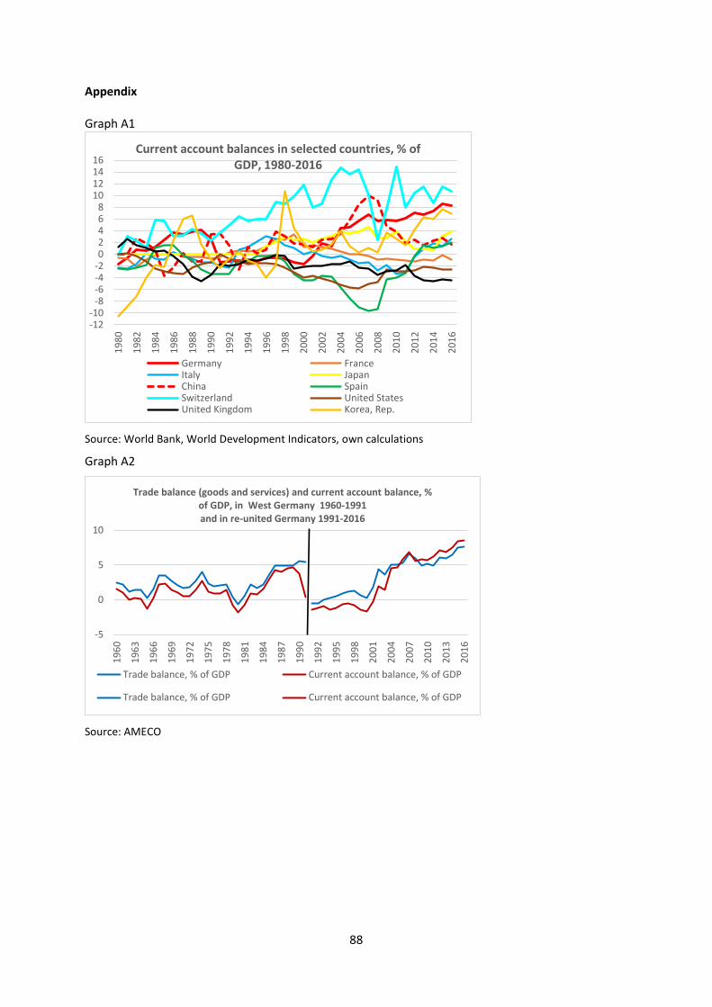
Appendix Graph A1
Source: World Bank, World Development Indicators, own calculations
Graph A2
Source: AMECO
-12-10
-8-6-4-202468
10121416
1980
1982
1984
1986
1988
1990
1992
1994
1996
1998
2000
2002
2004
2006
2008
2010
2012
2014
2016
Current account balances in selected countries, % of GDP, 1980-2016
Germany FranceItaly JapanChina SpainSwitzerland United StatesUnited Kingdom Korea, Rep.
-5
0
5
10
1960
1963
1966
1969
1972
1975
1978
1981
1984
1987
1990
1992
1995
1998
2001
2004
2007
2010
2013
2016
Trade balance (goods and services) and current account balance, % of GDP, in West Germany 1960-1991 and in re-united Germany 1991-2016
Trade balance, % of GDP Current account balance, % of GDP
Trade balance, % of GDP Current account balance, % of GDP
88
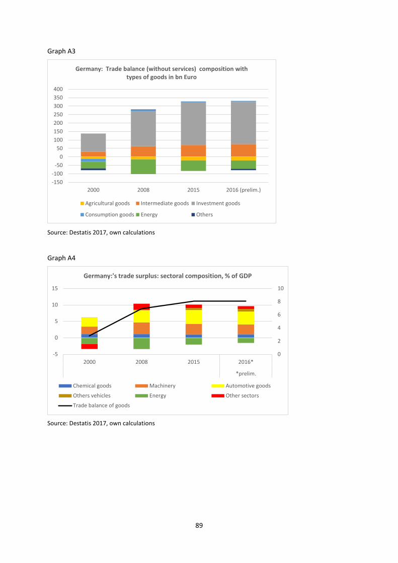
Graph A3
Source: Destatis 2017, own calculations
Graph A4
Source: Destatis 2017, own calculations
-150-100
-500
50100150200250300350400
2000 2008 2015 2016 (prelim.)
Germany: Trade balance (without services) composition with types of goods in bn Euro
Agricultural goods Intermediate goods Investment goods
Consumption goods Energy Others
0
2
4
6
8
10
-5
0
5
10
15
2000 2008 2015 2016*
*prelim.
Germany:'s trade surplus: sectoral composition, % of GDP
Chemical goods Machinery Automotive goods
Others vehicles Energy Other sectors
Trade balance of goods
89
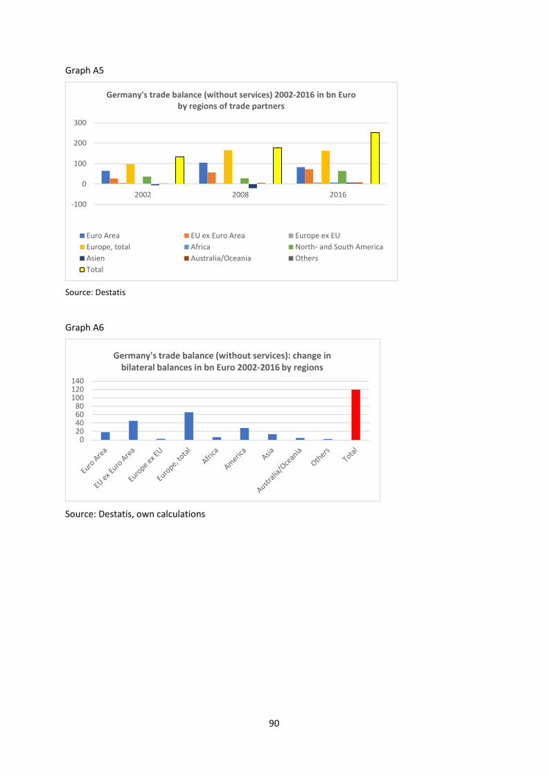
Graph A5
Source: Destatis
Graph A6
Source: Destatis, own calculations
-100
0
100
200
300
2002 2008 2016
Germany's trade balance (without services) 2002-2016 in bn Euro by regions of trade partners
Euro Area EU ex Euro Area Europe ex EUEurope, total Africa North- and South AmericaAsien Australia/Oceania OthersTotal
020406080
100120140
Germany's trade balance (without services): change in bilateral balances in bn Euro 2002-2016 by regions
90
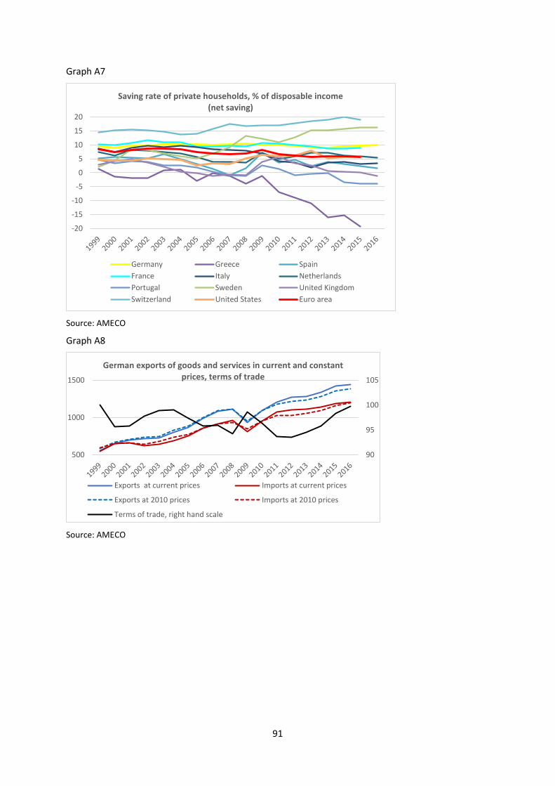
Graph A7
Source: AMECO
Graph A8
Source: AMECO
-20
-15
-10
-5
0
5
10
15
20
Saving rate of private households, % of disposable income (net saving)
Germany Greece SpainFrance Italy NetherlandsPortugal Sweden United KingdomSwitzerland United States Euro area
90
95
100
105
500
1000
1500
German exports of goods and services in current and constant prices, terms of trade
Exports at current prices Imports at current prices
Exports at 2010 prices Imports at 2010 prices
Terms of trade, right hand scale
91
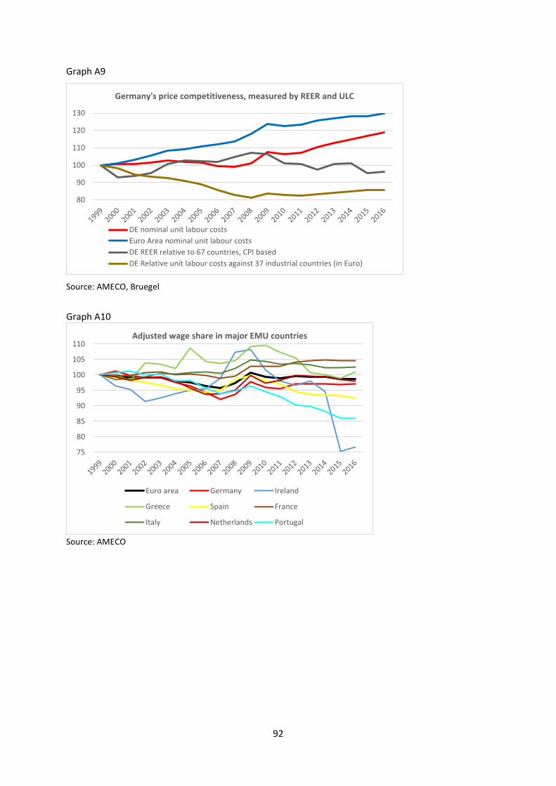
Graph A9
Source: AMECO, Bruegel
Graph A10
Source: AMECO
80
90
100
110
120
130
Germany's price competitiveness, measured by REER and ULC
DE nominal unit labour costsEuro Area nominal unit labour costsDE REER relative to 67 countries, CPI basedDE Relative unit labour costs against 37 industrial countries (in Euro)
75
80
85
90
95
100
105
110Adjusted wage share in major EMU countries
Euro area Germany Ireland
Greece Spain France
Italy Netherlands Portugal
92
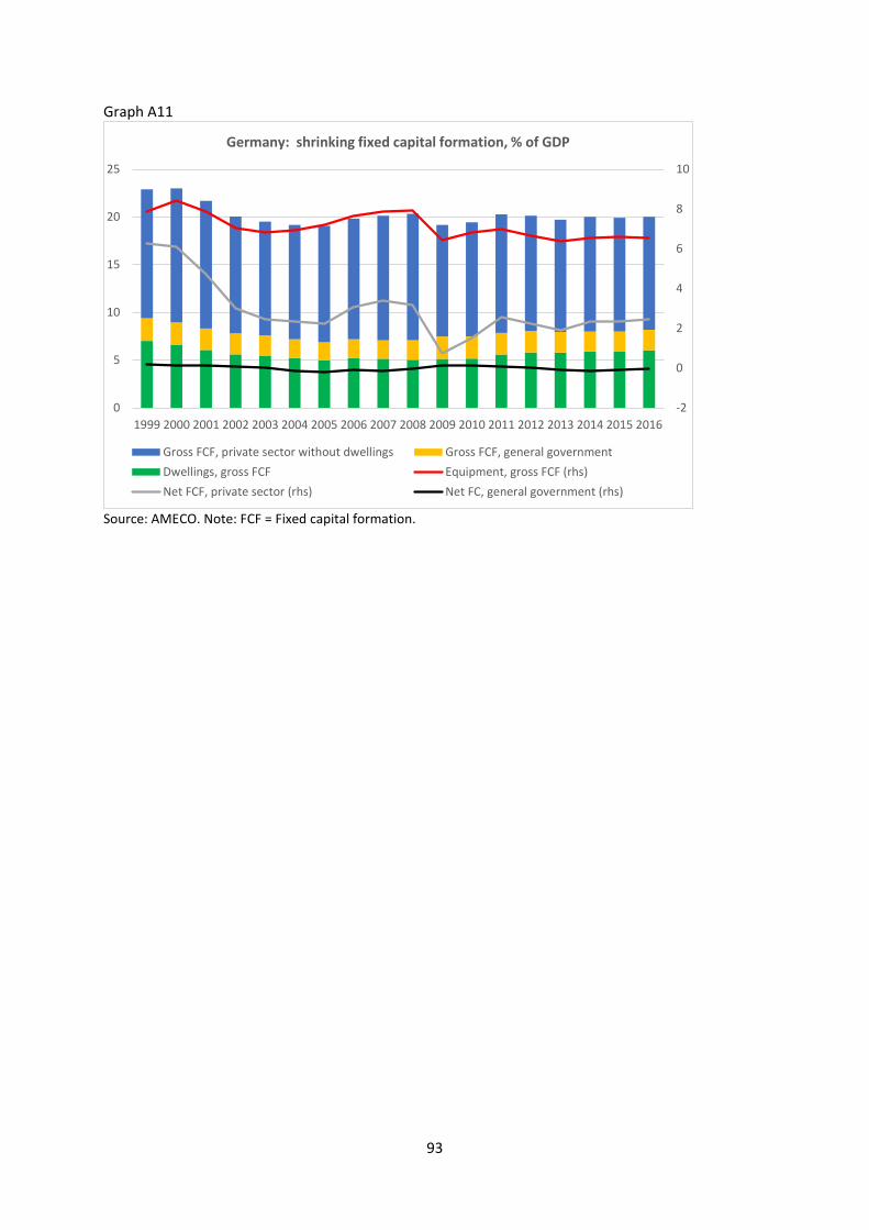
Graph A11
Source: AMECO. Note: FCF = Fixed capital formation.
-2
0
2
4
6
8
10
0
5
10
15
20
25
1999 2000 2001 2002 2003 2004 2005 2006 2007 2008 2009 2010 2011 2012 2013 2014 2015 2016
Germany: shrinking fixed capital formation, % of GDP
Gross FCF, private sector without dwellings Gross FCF, general governmentDwellings, gross FCF Equipment, gross FCF (rhs)Net FCF, private sector (rhs) Net FC, general government (rhs)
93

Graph A12
Source: AMECO
-10
0
10
20
1999
2000
2001
2002
2003
2004
2005
2006
2007
2008
2009
2010
2011
2012
2013
2014
2015
2016
Germany: Current account balance, as budget balance plus private sector balance, % of GDP
Budget balance private sector balance
-20-10
01020
1999
2000
2001
2002
2003
2004
2005
2006
2007
2008
2009
2010
2011
2012
2013
2014
2015
2016
Greece: Current account balance, as budget balance plus private sector balance, % of GDP
Budget balance private sector balance
-40
-20
0
20
40
1999
2000
2001
2002
2003
2004
2005
2006
2007
2008
2009
2010
2011
2012
2013
2014
2015
2016
Ireland: Current account balance, as budget balance plus private sector balance, % of GDP
Budget balance private sector balance
-15-10
-505
1015
1999
2000
2001
2002
2003
2004
2005
2006
2007
2008
2009
2010
2011
2012
2013
2014
2015
2016
Spain: Current account balance, as budget balance plus private sector balance, % of GDP
Budget balance private sector balance
94
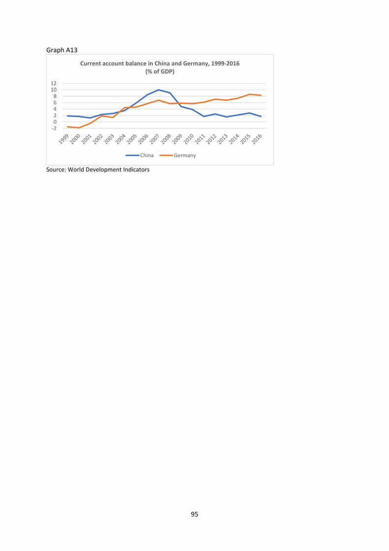
Graph A13
Source: World Development Indicators
-202468
1012
Current account balance in China and Germany, 1999-2016 (% of GDP)
China Germany
95
Impressum
Publisher: Hans-Böckler-Stiftung, Hans-Böckler-Str. 39, 40476 Düsseldorf, Germany Phone: +49-211-7778-331, [email protected], http://www.imk-boeckler.de
IMK Study is an online publication series available at: http://www.boeckler.de/imk_5023.htm
ISSN: 1861-2180 The views expressed in this paper do not necessarily reflect those of the IMK or the Hans-Böckler-Foundation. All rights reserved. Reproduction for educational and non-commercial purposes is permitted provided that the source is acknowledged.