A THREE LEVEL VULNERABILITY APPROACH FOR THE DAMAGE ... · A THREE LEVEL VULNERABILITY APPROACH FOR...

1

A THREE LEVEL VULNERABILITY APPROACH FOR

THE DAMAGE ASSESSMENT OF INFILLED RC

BUILDINGS: THE EMILIA 2012 CASE (V 1.0)

Gerardo Mario Verderame, Flavia De Luca, Maria Teresa De Risi, Carlo Del Gaudio, Paolo Ricci

[email protected], [email protected], [email protected], [email protected],

[email protected]

Dipartimento di Ingegneria Strutturale, Università degli Studi di Napoli Federico II.

Index

1 Introduction ............................................................................................................................................... 2

2 Emilia building stock and classification .................................................................................................... 3

2.1 Official statistical data on the building stock ........................................................................ 3

2.2 Evolution of the seismic classification in the Emilia region ................................................. 5

2.3 Benchmark structures ............................................................................................................ 7

3 Vulnerability apprOaches and earthquake damage assessment ................................................................. 9

4 EXACT vulnerability approach ................................................................................................................ 12

4.1 Simulated design procedure ................................................................................................ 12

4.2 Numerical model ................................................................................................................. 12

4.3 Analysis methodology ......................................................................................................... 14

4.4 Results ................................................................................................................................. 17

5 POST vulenrability approach ................................................................................................................... 19

5.1 Input data ............................................................................................................................. 20

5.2 Simulated design procedure ................................................................................................ 21

5.3 Characterization of nonlinear response ............................................................................... 22

5.4 Seismic assessment.............................................................................................................. 23

6 FAST vulnerability approach ................................................................................................................... 28

6.1 Simplified simulated design procedure ............................................................................... 29

6.2 Evaluation of the approximate capacity curve of RC infilled building ............................... 30

6.3 Seismic assessment.............................................................................................................. 33

7 Comparative damage assessment ............................................................................................................ 38

8 Conclusions and Perspectives .................................................................................................................. 45

Cite as: G.M. Verderame, F. De Luca, M.T. De Risi, C. Del Gaudio, P. Ricci (2012), A three level

vulnerability approach for damage assessment of infilled RC buildings: The Emilia 2012 case (V

1.0), available at http://www.reluis.it.

2

1 INTRODUCTION

On the 20th

of May the Emilia region was struck by a magnitude (Mw) 6.0 (according to USGS)

earthquake. The highest PGA registered at the closest station from the epicenter was equal to 0.27g

approximately (Chioccarelli et al, 2012a). The event involved a large area between the provinces of

Modena, Ferrara, Rovigo and Mantova. Main damage involved historical buildings, masonry

buildings, industrial structures, and in some cases also reinforced concrete structures, as shown by

in-filed reports after the earthquake (e.g., EPICentre Field Observation Report No. EPI-FO-200512,

2012; EPICentre Field Observation Report No. EPI-FO-290512, 2012; Decanini et al., 2012). The

mainshock was followed by a Mw 5.8 (according to INGV) aftershock on the 29th

of May

(Chioccarelli et al., 2012b) and the whole seismic sequence from the 16th

of May up to the 26th

of

June was characterized by seven events with magnitude equal or higher than 5.0

(http://www.ingv.it/it/).

Notwithstanding the fact that a single event cannot be employed to validate hazard data adopted

by codes for design and assessment (Iervolino, 2012), a comparison with ground motion prediction

equations and code spectra for the area can still be done (Iervolino et al, 2012). The preliminary

comparison with elastic and inelastic ground motion prediction equations (Bindi et al., 2011; De

Luca, 2011), and code spectra (DM 14/01/2008) provided right after the event (Chioccarelli et al,

2012a), showed that earthquake magnitude and location are consistent with the ranges considered

by the Italian national hazard data (i.e., Stucchi et al., 2011), and ground motion values are in

general agreement with prediction equation and code spectra.

According to the latter remarks, the observed damage after the event seems to be in some way

“unexpected”, especially if referred to reinforced concrete structures. On the other hand, looking

into the evolution of the seismic classification of the area, and crossing such information with the

characteristics of building stock, it can be observed that most representative reinforced concrete

buildings are designed for gravity loads and seldom have more than four storeys, (see section 2).

The general characteristics of the building stock and the seismic evolution of the code

classifications allow the definition of three benchmark buildings that can be considered as

representative structures for the application of an EMS-98 based (Grunthal, 1998) damage

assessment, developed at three different level, and based on infill damage state only, (see section 3).

The working hypotheses and damage assessment results for each level of vulnerability approach

applied to the Emilia region are provided in section 4, 5, and 6, respectively. First of all a detailed

static pushover based vulnerability approach is pursued (see section 4), in the following referred as

3

EXACT, (Ricci et al, 2012). Secondly the results obtained on the three benchmark buildings are

provided through a mechanical based vulnerability approach, suitable for large scale assessment

(see section 5), also known as POST (Ricci, 2010). Finally, damage assessment results based on an

empirical-mechanical approximated approach are shown (Gomez-Martinez et al., 2012, De Luca et

al. 2012), referred in the following as FAST, (see section 6). The latter can be suitable for rapid

large-scale assessment or for emergency management right after seismic events (e.g., Goretti and Di

Pasquale, 2006).

A comparison of the results of the three vulnerability approaches is shown in section 7, and

finally crossed with the Peak Ground Acceleration (PGA) shake map provided by INGV right after

the earthquake (http://www.ingv.it/it/).

2 EMILIA BUILDING STOCK AND CLASSIFICATION

The definition of the benchmark structures for the three level vulnerability approach is made

through a two step process. The first step is to analyze the official data in terms of number of

storeys and age of construction for the area struck by the earthquake. The second step is pursued

looking into the evolution of the seismic classification of the area.Official statistical data on the

building stock

Emilia–Romagna is one of the richest, most developed regions in Europe, and it has the third

highest “gross domestic product” per capita in Italy. Bologna, its principal city, has one of Italy's

highest quality of life indices and advanced social services. Indeed, almost 5% of the whole

building stock is constituted by buildings or group of buildings used as hotels, offices, commerce

and industry, communications and transport (Figure 1a), according to Istat data.

The Istat (Italian National Institute of Statistics) survey is a nation-wide census that provides

information on citizens, foreign, buildings and dwellings. In particular, in the “14th

general census

of the population and dwellings” (14° Censimento generale della popolazione e delle abitazioni,

ISTAT 2001) information about the number of storeys, as well as characteristic of residential

buildings, and in some cases even those non residential, are provided.

For instance, the availability of such data allows to carry out the statistics of buildings in terms

of number of storeys (one-, two-, three-storeys and four or more storeys buildings), age of

construction (typically with a decennial-rate) and building typologies (masonry or reinforced

concrete buildings) for the spatial unit, the so called cell. Nevertheless, due to confidentiality

requirements, these statistics were presented in an aggregate manner, in which the information is

not immediately recognizable as a function of the identified classes; for example, it is not possible

4

to get the number of reinforced concrete (RC) buildings in a cell, date back to a specific age of

construction and characterized by a given number of storeys. In the following the statistics for the

448 Municipality hit by the 2012 earthquake are shown, see Figure 1.

Among the whole building stock of the area struck by the earthquake only 20% is constituted by

RC (Figure 1b). Almost 75% of the buildings is characterized by a number of stories lower or equal

than two (Figure 1c). Regarding this latter aspect, it should be noted that the number of storeys is

referred to all the buildings and it can be inferred that among the 60% of the two storeys buildings

the main part is masonry. A uniform rate over the years with respect to the age of construction of

the buildings can be observed from data shown in Figure 1d. Data from Figure 1 allow to infer that

the RC building stock is characterized mostly by low to medium rise buildings (from to 2, up to 4

storeys) and almost 60% of them was realized between 1960 and 1980.

Pe

rce

nta

ge

Building TypologyHousing Industrial

0

20

40

60

80

100

Pe

rce

nta

ge

Building typeRC Masonry

0

20

40

60

80

100

Number of storeys

Perc

enta

ge

1 2 3 40

25

50

75

Age of Construction

Perc

enta

ge

<’1919−4546−6162−7172−8182−91>’910

5

10

15

20

25

Figure 1. Statistics for the 448 Municipality hit by the earthquake of 20th of May 2012: percentages with

respect to building typology (a), building type (b), number of storeys (c), age of construction (d).

5

2.2 Evolution of the seismic classification in the Emilia region

Seismic classification in Italy and in general in all seismically prone areas is quite often a result

of disastrous earthquakes. In Italy, the first classification was released in 1909 after the disastrous

earthquake of Reggio Calabria and Messina in 1908. Obviously such a classification was updated at

the knowledge of the time. After this first classification every five or ten years a new update of

seismic classification and code provisions were provided (Lai et al., 2009).

In recent years, four are the fundamental dates for the evolution of the seismic classification in

Italy: 1984, 1998, 2003, and 2008. In fact, after the Friuli (1976) and Irpinia (1980) disastrous

earthquakes, three different seismic categories were classified, and the third category, characterized

by a PGA equal to 0.04g, was firstly introduced. First and second categories were characterized by

a PGA equal to 0.10g and 0.06g, respectively (Ricci et al., 2011a). Such accelerations were

determined through the seismic coefficient S equal to 12, 9, and 6, and decreasing with the

increasing of the category form first to third. According to the latter classification (De Marco and

Marsan, 1986) most of the area struck by the 2012 Emilia earthquake was classified as non seismic

(Figure 2a).

Successively, in 1998, a reclassification proposal was provided by the Servizio Sismico

Nazionale. Such a classification was never adopted officially by any code but it is at the basis of the

classification made in 2003 (OPCM 3274, 2003) after the San Giuliano earthquake. The 2003

regulation document introduced also modern design rule such as the so called capacity design. On

the other hand, it should be noted that such rules worked as recommendation, since they have never

become compulsory, and it was still possible to design new structures according to the previous

building code (DM 16/01/1996).

According to 1998 classification the area struck by the 2012 earthquake was firstly classified as

seismic, in the so called third category (0.04g). Successively, in the classification of the OPCM

3274, the whole area was still in third category; on the other hand a design PGA of 0.15g on rigid

soil was employed; being the PGA with 10% probability of exceedance in 50 years of such areas

comprised in the range 0.05-0.15g.

The 2003 classification and the design provisions (OPCM 3274, 2003), even if they were not

compulsory, represented the “Copernican revolution” of Italian earthquake engineering, since it was

the first step towards the European unified design approach provided by Eurocodes and the first

introduction of modern seismic design rules. In particular, the OPCM 3274 (2003) was very similar

to the provisions provided in Eurocode 8 or EC8 (CEN, 2004).

6

The last step in terms of seismic classification was made in 2008, when the DM 14/01/2008 was

released. In the 2008 code the seismic input is based on specific hazard data based on a 5km spaced

grid (Stucchi et al., 2011) and spectral shape is site dependant, ending up in a code spectra very

close to a uniform hazard spectrum (UHS) PGA on rigid soil according to 2008 code are shown in

as shown in Figure 2b.

Toscana

Veneto

Lombardia

Emilia Romagna

Umbria

Marche

Trentino-Alto Adige

Liguria

Friuli-Venezia Giulia

Lazio

Piemonte

TRENTO

PERUGIA

SIENA

BRESCIA

PISA

PARMA

FIRENZE

AREZZO

BOLOGNA

VERONA

GROSSETO

VICENZA

MODENA

TREVISO

FERRARA

BERGAMO

VENEZIA

PADOVA

BELLUNO

PIACENZA

LUCCA

SONDRIO

MANTOVA

ROVIGO

PAVIA

TERNI

RAVENNA

PORDENONE

CREMONALODI

COMO

PESARO E URBINO

FORLI - CESENA

MILANO

PISTOIA

LECCO

GENOVA

RIMINI

UDINE

REGGIO NELL'EMILIA

LIVORNO

LA SPEZIA

ANCONA

MASSA - CARRARA

PRATO

MACERATA

VITERBO

BOLZANO

LIVORNO

UDINE

LegendClassification 1984

0

1

2

3

0 10 20 30 405

Kilometers

(a)

Toscana

Veneto

Lombardia

Emilia Romagna

Umbria

Marche

Trentino-Alto Adige

Liguria

Friuli-Venezia Giulia

Lazio

Piemonte

TRENTO

PERUGIA

SIENA

BRESCIA

PISA

PARMA

FIRENZE

AREZZO

BOLOGNA

VERONA

GROSSETO

VICENZA

MODENA

TREVISO

FERRARA

BERGAMO

VENEZIA

PADOVA

BELLUNO

PIACENZA

LUCCA

SONDRIO

MANTOVA

ROVIGO

PAVIA

TERNI

RAVENNA

PORDENONE

CREMONALODI

COMO

PESARO E URBINO

FORLI - CESENA

MILANO

PISTOIA

LECCO

GENOVA

RIMINI

UDINE

REGGIO NELL'EMILIA

LIVORNO

LA SPEZIA

ANCONA

MASSA - CARRARA

PRATO

MACERATA

VITERBO

BOLZANO

LIVORNO

UDINE

Legend

Classification 2008

0,036478 - 0,050863

0,050864 - 0,088864

0,088865 - 0,138260

0,138261 - 0,183143

0,183144 - 0,277300

0 10 20 30 405

Kilometers

(b)

Figure 2. Seismic classification before 1998, according to De Marco and Marsan (1986), (a); and actual

classification according to the official hazard data (Stucchi et al, 2011) employed in DM 14/01/2008, (b).

In Figure 3 the geological classification of the soil according to EC8 and the code spectra

according to OPCM 3274, EC8 and DM 14/01/2008 are evaluated for the epicenter of the event of

the 20th

of May. The only spectra according to actual Italian seismic code (DM 14/01/2008) is

dependent on the geographic coordinates and spectral shape depends on the probability of

exceedance considered (in this case 10% in 50 years), while both OPCM 3274 and EC8 spectra

depends on the seismic zone and soil class only. The value of PGA on rigid soil is equal to 0.138g

according to DM 14/01/2008, while it is equal to 0.15g in the case of OPCM and EC8. On the other

hand, the soil amplification factor for D soil type is 1.8 in the case of the Italian code and 1.35 in the

case of EC8 (type 1) and OPCM. Soil D was chosen for this code spectral comparison because it is

the most frequent class in the whole epicentral area. In the following all spectral based approaches

7

are going to be pursued considering the EC8 spectra in Figure 3b. Given the fact they are similar, it

is preferable to consider a single spectra that in some way accounts for the general characteristics of

the vast area struck by the earthquake.

0 1 2 30

0.2

0.4

0.6

0.8

1

T [s]

Sa(T

) [g

]

OPCM & EC8NTC2008

(a) (b)

Figure 3. Soil classification on geological basis of the area struck by the earthquake (a); comparison of

code spectra according to EC8, OPCM 3274, and DM14/01/2008 for D soil class at the epicenter of the event

of the 20th of May (lat. 44.89, long. 11.23), (b).

It should be finally noted that the 2008 code became the official Italian code and the only one to

be employed only in July 2009, after the 2009 L’Aquila earthquake.

According to the previous observations, and considering that most of the building stock was

realized between sixties and eighties it is easy to recognize that most of the area stuck by the 2012

Emilia earthquake was designed for gravity loads. Another support reason for the choice of gravity

load designed structures as representative of the whole RC building stock of the area is that in the

case of mid rise RC buildings and medium-low seismicity design the gravity loads still rule the

design, as long as capacity design is not employed (e.g., Benavent-Climent, 2004).

2.3 Benchmark structures

Data and information in the previous section allow the definition of the benchmark structures

employed in this study. The structures analyzed are symmetric in plan, both in longitudinal (X) and

8

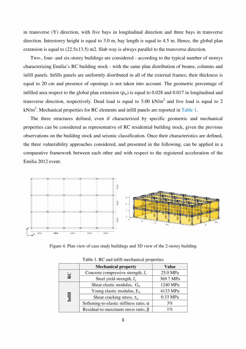
in transverse (Y) direction, with five bays in longitudinal direction and three bays in transverse

direction. Interstorey height is equal to 3.0 m, bay length is equal to 4.5 m. Hence, the global plan

extension is equal to (22.5x13.5) m2. Slab way is always parallel to the transverse direction.

Two-, four- and six-storey buildings are considered - according to the typical number of storeys

characterizing Emilia’s RC building stock - with the same plan distribution of beams, columns and

infill panels. Infills panels are uniformly distributed in all of the external frames; their thickness is

equal to 20 cm and presence of openings is not taken into account. The geometric percentage of

infilled area respect to the global plan extension (ρw) is equal to 0.028 and 0.017 in longitudinal and

transverse direction, respectively. Dead load is equal to 5.00 kN/m2 and live load is equal to 2

kN/m2. Mechanical properties for RC elements and infill panels are reported in Table 1.

The three structures defined, even if characterized by specific geometric and mechanical

properties can be considered as representative of RC residential building stock, given the previous

observations on the building stock and seismic classification. Once their characteristics are defined,

the three vulnerability approaches considered, and presented in the following, can be applied in a

comparative framework between each other and with respect to the registered acceleration of the

Emilia 2012 event.

4.5 m 4.5 m4.5 m 4.5 m 4.5 m 4.5 m

4.5

m4

.5 m

4.5

m

X

Y

Figure 4. Plan view of case study buildings and 3D view of the 2-storey building

Table 1. RC and infill mechanical properties

Mechanical property Value

RC

Concrete compressive strength, fc 25.0 MPa

Steel yield strength, fy 369.7 MPa

Infi

ll

Shear elastic modulus, Gw 1240 MPa

Young elastic modulus, Ew 4133 MPa

Shear cracking stress, τcr 0.33 MPa

Softening-to-elastic stiffness ratio, α 3%

Residual-to-maximum stress ratio, β 1%

9

3 VULNERABILITY APPROACHES AND EARTHQUAKE DAMAGE ASSESSMENT

Vulnerability represents with the so called exposure the part of seismic risk in which engineers,

practitioners, and governments can play a crucial role. The first depends on the main characteristics

of the building stock, and the design rules according to which such building stock was realized. The

study and the interpretation of structural behaviour become crucial in prevention, mitigation, and

after earthquake management. Each of the latter actions ask for different level of detailing and

accuracy in the approach.

The main framework of vulnerability approaches can be divided in three main groups: (i)

approaches that select a representative building of the building stock to be studies and consider only

the intra-building variability (e.g., Rossetto and Enlnashai, 2005); (ii) approaches that analyze

building classes considering directly both intra- and inter-building variability so introducing

uncertainties within the class of structures (e.g., Cosenza et al, 2005; Iervolino et al., 2007; Ricci,

2010); (iii) approaches based on both mechanical and empirical basis that define approximately the

capacity curve (e.g., Giovinazzi and Lagomarino, 2004; Giovinazzi, 2005).

The two approximate approaches for large scale assessment provided herein can be respectively

collocated in the second and third group; in fact the POST continues, by means of the introduction

of structural infill contribution, the ideal outline of building classes vulnerability approaches; while

the FAST provides a rapid assessment on a hybrid mechanical- empirical basis and it is ideally close

to the third group of approaches.

All the vulnerability approaches end up in a comparison with observed damage data collected

after earthquakes. The collection of damage data asks for an objective classification of the damage

for each building type. In this framework the macro seismic intensity scale plays a significant role.

Macro seismic intensity scales classify the severity of an earthquake by means of damages

induced on civil structures and on territory. The most utilized in Europe are the Mercalli Scale,

dating at the beginning of ‘900, which through a series of modification and improvement gave rise

to the Mercalli-Cancani-Sieberg Scale, and the European Macroseismic Scale (EMS).

EMS is the basis for evaluation of seismic intensity in European countries and it is also used in a

number of countries outside Europe. Issued in 1998 as an update of the test version from 1992, the

scale is referred to as EMS-98 (Grunthal, 1998). A different classification of damage is provided for

masonry and infilled RC structures.

The EMS-98 scale involves five grades of damage (in the following they are referred as DSi)

from slight damage up to destruction, passing trough moderate, heavy and vey heavy damage. For

each level an increasing characterization of damage to masonry infills (nonstructural elements) and

10

RC elements (structural elements) is provided, each single DS is characterized by a classification of

both structural and non-structural damage.

In second column of Table 2 is reported the classification of the first three DS for RC buildings

described in EMS-98 and the mechanical interpretation relative to displacement thresholds in

secondary elements.

Table 2. RC and infill mechanical properties

Grade 1: Negligible to slight damage (no structural damage, slight non-

structural damage) DS 1:

Fine cracks in plaster over frame members or in walls at the base.

Fine cracks in partitions and infills.

inf

cr∆

Grade 2: Moderate damage (slight structural damage, moderate non-


Cracks in columns and beams of frames

and in structural walls. Cracks in partition and infill walls; fall of brittle cladding and plaster. Falling mortar from the joints of wall panels.

inf

max∆

Grade 3: Substantial to heavy damage (moderate structural damage, heavy non-


Cracks in columns and beam column

joints of frames at the base and at joints

of coupled walls.

Spalling of concrete cover, buckling of reinforced rods.

Large cracks in partition and infill walls,

failure of individual infill panels.

inf

u∆

Drift

Norm

aliz

ed F

orc

e (

F/F

max)

0 0.002 0.004 0.006 0.008 0.010

0.2

0.4

0.6

0.8

1

1.2

The definition of the Damage State (DS) has been carried out interpreting and translating

through engineering judgment the qualitative terms, fine cracks, cracks and large cracks for non-

structural elements, presented in EMS-98 into displacement threshold related to non linear behavior

of infills. In particular a building is classified in Grade 1 (DS1) if it exhibits fine cracks in infills.

This condition corresponds into mechanical model of building to the overtaking of the cracking

displacement to the envelope of infills. Instead Grade 2 and 3, characterize by an increasing level of

damage, can be associated to the displacement relative to maximum infills resistance and by the

failure of infill, respectively. Figure 5 shows an example of DS1, DS2 and DS3, specifically

referred to infills damage classification provided in Table 2; such damage have been observed after

the 2012 Emilia earthquake.

11

(a) (b)

(c)

Figure 5. Example of damage to infills during the 2012 Emilia earthquake that can be representative of DS1

[from Decanini et al., 2012] (a), DS2, [from EPICentre Field Observation Report No. EPI-FO-290512, 2012]

(b), and DS3 [taken by Flavia De Luca] (c).

12

4 EXACT VULNERABILITY APPROACH

In the following the adopted detailed or EXACT vulnerability analysis approach will be

illustrated: the simulated design procedure is explained in section 4.1; the adopted numerical model

is presented in section 4.2; analysis methodology and obtained results are illustrated in 4.3 and 4.4,

respectively.

4.1 Simulated design procedure

Element dimensions are defined through a simulated design procedure according to code

prescriptions and design practices in force in Italy between 1950s and 1970s (Regio Decreto Legge

n. 2229, 16/11/1939; Verderame et al., 2010a). The structural configuration follows the parallel

plane frames system: gravity loads from slabs are carried only by frames in longitudinal direction.

Beams in transverse direction are not present in the internal frames. Element dimensions are

calculated according to the allowable stresses method; the design value for maximum concrete

compressive stress is assumed equal to 5.0 and 7.5 MPa for axial load and axial load combined with

bending, respectively. Column dimensions are calculated according only to the axial load based on

the tributary area of each column; beam dimensions and reinforcement are determined from

bending due to loads from slabs. Reinforcing bars are smooth and their allowable design stress is

equal to 160 MPa. Section dimensions are (30x50) cm2 for beams, whereas they are strongly

variable for columns, depending on the design axial load and on the selected shape – in this

approach column can have square or rectangular section.

4.2 Numerical model

Nonlinear response of RC elements is modeled by means of a lumped plasticity approach:

beams and columns are represented by elastic elements with nonlinear rotational hinges at the ends.

A three-linear envelope is used, where characteristic points are cracking, yielding and ultimate.

Section moment and curvature at cracking and yielding are calculated on a fiber section, for an axial

load value corresponding to gravity loads. The behavior is assumed linear elastic up to cracking and

perfectly-plastic after yielding. Rotations at yielding and ultimate are evaluated through the

formulations given in (Fardis, 2007). No reduction of ultimate rotation for the lack of seismic

detailing is applied, due to the presence of smooth reinforcement (Verderame et al., 2010b).

Infill panels are modeled by means of equivalent struts. Modeling infills through single

compressed struts allow to investigate on the effect of the panels on the global behavior of the

analyzed structure (highlight possible brittle failure due to interaction between infill panels and the

13

surrounding RC elements is beyond the purpose of this paper). The adopted model for the envelope

curve of the force-displacement relationship is the model proposed by Panagiotakos and Fardis

(Panagiotakos and Fardis, 1996; Fardis, 1997). The proposed force-displacement envelope is

composed by four branches, as shown in Figure . The first branch corresponds to the linear elastic

behavior up to cracking; the slope of this branch is the elastic stiffness of the infill panel kel, and it

can be expressed according to Equation (1), being Aw is the transversal area of the infill panel, Gw

the shear elastic modulus and hw its clear height. If τcr is the shear cracking stress, the shear

cracking strength Fcr can be obtained according to Equation (2).

w w

el

w

G AK

h=

(1)

cr cr wF Aτ= (2)

The second branch continues up to the maximum strength Fmax, which can be calculated

according to Equation (3). The corresponding displacement ∆max is estimated in the hypothesis that

secant stiffness up to maximum is provided by Mainstone’s formulation (Mainstone, 1971),

assuming that width of the equivalent truss bw is according to Equation (4), being hw and dw the

height and the diagonal length of the truss, respectively, and λh is defined according to Equation

(5). In Equation (5), Ew and Ec are the elastic Young modulus of the infill panel and of the

surrounding concrete, respectively; θ is the diagonal slope of the equivalent truss; tw is the infill

thickness; Ic is the moment of inertia of the adjacent columns. Secant stiffness up to maximum is

equal to the expression shown in Equation (6).

(∆ , F =1.30 F

(∆ cr ,Fcr )

Axial force, F

Axial , ∆

(∆u ,Fu

(Ew b w tw /d w)

(∆max cr )

∆ )

dis placement , ∆

(∆ ,F

( )

K el =0.01F )max

max

0.03 K el

Drift

Norm

aliz

ed F

orc

e (

F/F

max)

0 0.002 0.004 0.006 0.008 0.010

0.2

0.4

0.6

0.8

1

1.2

Figure 6. Panagiotakos and Fardis single-strut infill model

14

max 1.30cr

F F= ⋅ (3)

( )0.4

0.175w h w wb h dλ−

= (4)

4sin(2 )

4

w w

h

c c w

E t

E I h

θλ =

(5)

sec2 2

cosw w wE b tK

L Hθ=

+ (6)

The third branch of the infill envelope is a degrading branch up to the residual strength of the

infill panel; its slope (kdeg) depends on the elastic stiffness through the parameter α. In literature,

authors suggest values in the range [0.005; 0.1] for the parameter α, see Equation (7). Last branch is

horizontal; it corresponds to a residual constant strength; residual-to-maximum strength ratio β can

be assumed equal to 1-2% (Panagiotakos and Fardis, 1996; Dolsek and Fajfar, 2004a). In this

report, the ratio between post-capping degrading stiffness and elastic stiffness (parameter α) is

assumed equal to 0.03 (Panagiotakos and Fardis, 1996). The ratio between residual strength and

maximum strength (parameter β) is assumed equal to 0.01 (Dolsek and Fajfar, 2004a).

deg elK Kα= − (7)

4.3 Analysis methodology

Nonlinear static push-over (SPO) analyses are performed on the benchmark buildings both in X

and Y direction: the assumed lateral load pattern is proportional to the displacement shape of the

first mode and lateral response is evaluated in terms of base shear-top displacement relationship.

Structural modeling and numerical analyses are performed through the “PBEE toolbox” software

(Dolšek, 2010), combining MATLAB® with OpenSees (McKenna et al., 2004), modified in order

to include also infill elements (Ricci, 2010; Celarec et al., 2012).

The lateral response is characterized by a strength degradation due to infill failure; thus a multi-

linearization of the pushover curve is necessary and it is carried out by applying the equal energy

rule respectively between the initial point and the maximum resistance point, and between the point

corresponding to the last infill failure and the point corresponding to the first RC element

conventional collapse.

Starting from the multi-linearized capacity curves, IN2 curves (Dolšek and Fajfar, 2008) for the

equivalent SDoF systems are obtained by assuming as Intensity Measure (IM) both the elastic

15

spectral acceleration at the period of the equivalent SDoF system (Sae(Teff)) and the PGA. An IN2

curve, such as an IDA curve, is a relationship between a Demand Parameter (EDP), e.g. top

horizontal displacement, and an IM, e.g. elastic spectral acceleration for a certain period or PGA. If

an IN2 curve in terms of top displacement versus PGA is considered, the PGA corresponding to a

certain value of top displacement represents the PGA capacity of the structure for that displacement.

Thus, the seismic capacity expressed in terms of PGA is defined as the PGA corresponding to the

demand spectrum under which the displacement demand is equal to the displacement capacity. In

the same way, seismic capacity expressed in term of Sae(Teff) can be defined.

Values of Sae(Teff) and PGA corresponding to characteristic values of displacement (ductility)

demand (including the considered DSs) are calculated, based on the R-µ-T relationships given in

(Dolšek and Fajfar, 2004a) for degrading response (Figure 7). It is worth noting that this relation is

intended to be used with an idealized elastic spectrum of the Newmark-Hall type.

The strength reduction factor R can be defined as the ratio between the elastic spectral

acceleration corresponding to the effective period Sae and the yielding acceleration Say of the

equivalent SDoF. The ductility µ can be expressed as a function of R as shown in Equation (8).

Hence, in the proposed R-µ-T relationship, the ductility µ is linearly dependent on R-factor; the

parameter c defines the slope of the R-µ relationship and it depends on the effective period of the

structure, the minimum-to-maximum strength ratio ru and on the characteristic periods of the ground

motion TC and TD (Dolšek and Fajfar, 2004a). Equation (8) can be rewritten in the form of Equation

(9), which can be used for the determination of reduction factors for a given ductility.

( )0 0

1R R

cµ µ= − +

(8)

( )0 0R c Rµ µ= − + (9)

The proposed R-µ-T relationship has been validated only to a maximum value of the ductility at

the beginning of degradation µs equal to 2.5 and to a minimum value of ru equal to 0.25, which may

represent some limits of applicability of this law. The central value can be calculated either for the

ductility µ at a given reduction factor R or for the reduction factor R for a given ductility µ. These

two approaches can lead to different results (Chopra and Chintanapakdee, 2003). In (Dolšek and

Fajfar, 2004a), authors demonstrate that the proposed R-µ-T relationship yields larger ductilities for

a given reduction factor and, if inverted, a smaller reduction factor for a given ductility, thus

16

proving the conservativeness of this relation both for performance assessment and design.

Furthermore, the authors proved that the ductility at the end of strength degradation µu has a

negligible influence on the reduction factor R, thus this parameter is not included in the proposed

law. The ductility at the beginning of degradation µs and the residual-to-maximum strength ratio ru

are essential for the proposed R-µ-T relationship and, thus, IN2 curves are strictly dependent on the

parameters µs and ru of the multi-linearized capacity curves.

Moreover, the procedure proposed in (Dolšek and Fajfar, 2005) to improve the accuracy of the

displacement demand assessment in the case of low seismic demand is applied. The N2 method is

not intended to be used for structures which remain in the (equivalent) elastic region. However, one

may wish to compute realistic displacement demand also for acceleration demand Sae(T), which is

lower than the yield acceleration Say of the idealized pushover curve, i.e. for R<1. This goal can be

obtained by approximating the first part of the pushover curve by a bilinear curve rather than a

linear one and applying specific R-µ-T relationship in this range of behavior, as proposed by Dolsek

and Fajfar. The two parts of the bilinear curve are separated by the point (De; Fe) , which represents

the boundary of the initial ideal elastic behavior, and is arbitrarily defined as the crossing point of

the radial line with a slope equal to 95% of the initial stiffness of the structure with the computed

pushover curve. This improvement of accuracy is applicable to any structural system which is

characterized by a pushover curve that substantially deviates from a line in the equivalent elastic

region. Elastic spectra used for the construction of the IN2 curves are the demand spectra adopted in

Eurocode 8 – type A – for a soil type D (see Figure 3).

0 1 2 3 4 50

2

4

6

8

T/TC

R|µ

µ = 2

µ = 3

µ = 4

µ = 6

0 1 2 3 4 50

2

4

6

8

10

T/TC

µ|R

R = 2R = 3R = 4R = 6

Figure 7. Adopted R-µ-T relationship for infilled frames with ru=0.4, µs=2.5, TC=0.8s, TD=2s

17

4.4 Results

Pushover curves are obtained for the case study buildings in both longitudinal and transverse

directions; two- and four-storey case study buildings show a collapse mechanism involving the only

first storey in both directions; six-storey building shows a collapse mechanism involving the only

second floor in longitudinal direction and first and second floors in the transverse one.

Capacity curves and IN2 curves in terms of Sea(Teff) – obtained as explained above – are reported in

Figure 8 for each benchmark structure. Capacity curves parameters are also summarized in Table 3,

where:

- Tel is the elastic period of the structure;

- Teff is the effective period of the structure;

- µs is the ductility at the beginning of the degradation;

- Cs,max is the maximum strength of the equivalent SDoF system, before the strength degradation

due to infills;

- Cs,min is the minimum strength of the equivalent SDoF system, after the strength degradation

due to infills;

- ru is the residual-to-maximum strength ratio;

- M* is the effective mass.

Moreover, seismic capacity expressed in term of Sae(Teff) is reported for each DS and for each case

study. Finally, in Table 4, displacement capacities of the equivalent SDoF corresponding to the

achievement of the analyzed DSs are reported.

Table 3. Capacity curves parameters and Sae(Teff) capacity – Detailed approach

Number

of

storeys

direction

Capacity curves’ parameters Sae(Teff) capacity

Tel Teff µµµµs Cs,max Cs,min ru M* DS1 DS2 DS3

[s] [s]

[g] [g]

[t] [g] [g] [g]

2 x 0.0818 0.1088 2.5649 0.9501 0.1999 0.2104 364 0.5537 1.0475 1.1261

y 0.1056 0.1438 2.8602 0.5863 0.1815 0.3096 370 0.3222 0.6605 0.8046

4 x 0.1467 0.1878 3.0368 0.5446 0.2129 0.391 633 0.2690 0.6457 0.8121

y 0.2013 0.2525 2.8123 0.3294 0.1477 0.4485 604 0.1540 0.4100 0.5434

6 x 0.2201 0.2675 3.3837 0.3857 0.2368 0.6139 879 0.1751 0.4615 0.6914

y 0.3074 0.3435 2.1102 0.2169 0.0992 0.4574 841 0.1078 0.2788 0.3843

Table 4. Displacement capacity of the equivalent SDoF – Detailed approach

Sd DS1 DS2 DS3 Sd DS1 DS2 DS3

Direction

x [cm] [cm] [cm]

Direction

y [cm] [cm] [cm]

2 storeys 0.098 0.581 3.161 2 storeys 0.101 0.604 3.201

4 storeys 0.158 1.017 3.183 4 storeys 0.168 1.100 3.960

6 storeys 0.225 1.262 3.509 6 storeys 0.258 1.240 3.396

18

2 Storey − Longitudinal IN2

Sd [m]

Sa(T

) [g

]

(a)

0 0.02 0.04 0.06 0.08 0.10

0.2

0.4

0.6

0.8

1

1.2

2 Storey − Transversal IN2

Sd [m]

Sa(T

) [g

]

(b)

0 0.02 0.04 0.06 0.08 0.10

0.2

0.4

0.6

0.8

1

1.2


Sd [m]

Sa(T

) [g

]

(c)

0 0.02 0.04 0.06 0.08 0.10

0.2

0.4

0.6

0.8

1

1.2


Sd [m]

Sa(T

) [g

](d)

0 0.02 0.04 0.06 0.08 0.10

0.2

0.4

0.6

0.8

1

1.2


Sd [m]

Sa(T

) [g

]

(e)

0 0.02 0.04 0.06 0.08 0.10

0.2

0.4

0.6

0.8

1

1.2


Sd [m]

Sa(T

) [g

]

(f)

0 0.02 0.04 0.06 0.08 0.10

0.2

0.4

0.6

0.8

1

1.2

Figure 8. Multi-linearized capacity curves and IN2 curves in terms of Sae(Teff) – Detailed approach

19

5 POST VULENRABILITY APPROACH

POST (PushOver on Shear Type models) is a simplified method for vulnerability assessment of

reinforced concrete buildings, employing a simulated design procedure to evaluate the building

structural characteristics based on few data such as number of storeys, global dimensions and type

of design, and on the assumption of a Shear Type behavior to evaluate in closed form the non-linear

static response. Hence, the N2 method is applied and the seismic capacity in terms of elastic

spectral acceleration at the period of the equivalent SDOF system and of the corresponding Peak

Ground Acceleration is evaluated, based on the displacement (ductility) capacity at the Damage

State of interest. POST is implemented in MATLAB® code, including a user interface, (see Figure

9).

Figure 9. POST user interface.

20

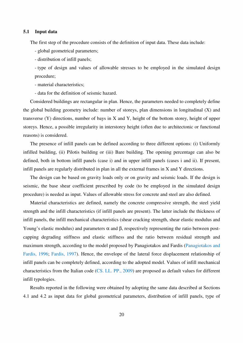
5.1 Input data

The first step of the procedure consists of the definition of input data. These data include:

- global geometrical parameters;

- distribution of infill panels;

- type of design and values of allowable stresses to be employed in the simulated design

procedure;

- material characteristics;

- data for the definition of seismic hazard.

Considered buildings are rectangular in plan. Hence, the parameters needed to completely define

the global building geometry include: number of storeys, plan dimensions in longitudinal (X) and

transverse (Y) directions, number of bays in X and Y, height of the bottom storey, height of upper

storeys. Hence, a possible irregularity in interstorey height (often due to architectonic or functional

reasons) is considered.

The presence of infill panels can be defined according to three different options: (i) Uniformly

infilled building, (ii) Pilotis building or (iii) Bare building. The opening percentage can also be

defined, both in bottom infill panels (case i) and in upper infill panels (cases i and ii). If present,

infill panels are regularly distributed in plan in all the external frames in X and Y directions.

The design can be based on gravity loads only or on gravity and seismic loads. If the design is

seismic, the base shear coefficient prescribed by code (to be employed in the simulated design

procedure) is needed as input. Values of allowable stress for concrete and steel are also defined.

Material characteristics are defined, namely the concrete compressive strength, the steel yield

strength and the infill characteristics (if infill panels are present). The latter include the thickness of

infill panels, the infill mechanical characteristics (shear cracking strength, shear elastic modulus and

Young’s elastic modulus) and parameters α and β, respectively representing the ratio between post-

capping degrading stiffness and elastic stiffness and the ratio between residual strength and

maximum strength, according to the model proposed by Panagiotakos and Fardis (Panagiotakos and

Fardis, 1996; Fardis, 1997). Hence, the envelope of the lateral force displacement relationship of

infill panels can be completely defined, according to the adopted model. Values of infill mechanical

characteristics from the Italian code (CS. LL. PP., 2009) are proposed as default values for different

infill typologies.

Results reported in the following were obtained by adopting the same data described at Sections

4.1 and 4.2 as input data for global geometrical parameters, distribution of infill panels, type of

21

design and values of allowable stresses to be employed in the simulated design procedure, and

material characteristics.

5.2 Simulated design procedure

The simulated design procedure adopted herein (Verderame et al., 2010a) is based on the

compliance with past code prescriptions and design practices for Italian RC buildings. Hence, the

allowable stresses method is followed.

First, design loads are defined. As far as gravity loads are concerned, dead loads are evaluated

from a load analysis, whereas live loads are evaluated from past code prescriptions for ordinary

structures (e.g., 2 kN/m2). Lateral loads (evaluated if the selected type of design is “seismic”) are

calculated based on the assigned base shear coefficient (ratio between the design base shear and the

weight of the structure). Typical values for this coefficient were, for instance, 0.07 or 0.10,

according to the category of the seismic zone.

Then, element dimensions are evaluated. To this aim, according to past design practices, column

area is determined as the ratio between the axial load (evaluated referring to the area of influence of

each column) and the allowable stress of concrete. In seismic design, the latter was typically

multiplied by a coefficient γ lower than 1, roughly accounting for combined axial load and bending

action acting on the column due to lateral loads (Pecce et al., 2004). Hence, γ was typically assumed

equal to 1 in gravity load design. Coefficient γ is given as an input for the simulated design

procedure. The column section is then determined from the calculated area, starting from a width

equal to 30 cm and considering a maximum height of 70 cm. If the calculated area is higher than

cm2, column width is increased from 30 to 35 cm, and so on. An upper approximation of 5 cm is

considered for the determination of section height. The beam width is given equal to 30 cm and the

corresponding height is calculated based on the maximum bending moment acting on the beam for

gravity loads from slabs; this moment is calculated with a formulation accounting in a simplified

way for the element constraint scheme. Finally, column dimensions are checked to avoid cross-

section variation higher than 10 cm between two adjacent storeys.

Once column and beam dimensions have been calculated, reinforcement in columns is designed.

Beam reinforcement is not designed since in the assumed Shear Type model the behavior of beam

elements has not to be modeled.

As far as gravitational design is concerned, the design of column reinforcement is based on the

minimum amount of longitudinal reinforcement geometric ratio prescribed by code (e.g., 0.8% of

the minimum concrete area according to RDL 2229 (1939), or 0.6% according to DM 3/3/1975)).

22

Once the minimum area of reinforcement has been determined, a set of possible values of bar

diameter is considered and the combination of (even) number and diameter of bars providing the

best upper approximation is chosen. Hence, bars are distributed along the periphery of the section as

uniformly as possible.

In seismic design, storey shear forces are evaluated from lateral forces, which are calculated as a

fraction of the weight of the structure, based on the assigned base shear coefficient. Hence, the

distribution of the storey shear among the columns of the storey is based on the ratio of inertia of

the single column versus the sum of inertia of all the columns at the considered storey (Shear Type

element model). The bending moment acting at the ends of each column is obtained multiplying the

corresponding shear force by half of the column height, according to the assumed Shear Type

model; the axial load is calculated from gravity loads, given by the sum of gravity loads and of a

fraction of live loads (30%), always based on the area of influence of the column. Then, based on

the assigned values of allowable stress for steel and concrete, the reinforcement area is designed to

provide a flexural strength (according to the allowable stresses method) not lower than the bending

moment from design. Again, the combination of number and diameter of bars providing the best

upper approximation is chosen provided at least two bars per layer. The described procedure is

carried out in both directions. Hence, the total amount of longitudinal reinforcement is compared

with the minimum amount prescribed by the considered code; the maximum between these values is

assumed.

5.3 Characterization of nonlinear response

Based on the assumed Shear Type model, the lateral response of the structure under a given

distribution of lateral forces can be completely determined based on the interstorey shear-

displacement relationships at each storey. Hence, the nonlinear response of column and infill

elements has to be determined.

The nonlinear behavior of each column element is characterized as a ( )T ∆ relationship

evaluated from the corresponding ( )M θ relationship, consistent with the Shear Type assumption.

The moment-rotation envelope is calculated assuming a shear span equal to half of the column

height (LV = h/2). A tri-linear envelope for is assumed, with three characteristic points: cracking,

yielding and ultimate condition. Behavior is linear elastic up to cracking and perfectly-plastic after

yielding.

Moment and rotation at cracking are evaluated based on first principles, assuming a linear

elastic section behavior up to this point.

23

Moment and section curvature at yielding are calculated in closed form by means of the first

principles-based simplified formulations proposed in (Biskinis and Fardis, 2010). Hence, rotations

at yielding (θy) and ultimate (θu) are evaluated according to (Biskinis and Fardis, 2010) and

(Biskinis and Fardis, 2010), respectively. The type of reinforcement is given as input, too; if smooth

bars are present, no reduction for the lack of seismic detailing is applied (Verderame et al., 2010b).

Then, the relationship between the displacement and the shear for each column is evaluated from

the relationship between the chord rotation and the end moment

Lateral force-displacement relationships for infill panels are evaluated from the model proposed

by Panagiotakos and Fardis (Panagiotakos and Fardis, 1996; Fardis, 1997), based on previously

defined data (panel thickness, infill mechanical characteristics and model parameters α and β) and

evaluating clear dimensions of the panel considering section dimensions of surrounding beams and

columns.

At each storey, the relationship between the interstorey displacement and the corresponding

interstorey shear is evaluated considering all the RC columns and the infill elements (if present)

acting in parallel. To this aim, displacement values corresponding to characteristic points of lateral

force-displacement envelopes of RC columns and infill elements are sorted in a vector; then, for

each of these displacement values the corresponding shear forces provided by each element are

evaluated and summed. In this way, a multi-linear storey shear-displacement relationship is

obtained. The illustrated procedure is carried out in both building directions.

5.4 Seismic assessment

Once the interstorey shear-displacement relationship at each storey has been defined, the base

shear-top displacement relationship representing the lateral response of the Shear Type building

model – under a given distribution of lateral forces – can be evaluated through a closed-form

procedure.

First, the fundamental period of vibration and the corresponding lateral displacement shape are

evaluated by means of an eigenvalue analysis. To this aim, mass and stiffness matrices of the Shear

Type model are easily constructed; elastic stiffness at each storey is calculated as the ratio between

force and displacement values corresponding to the first point of the multi-linear envelope

representing the interstorey shear-displacement relationship.

Hence, a linear, uniform or 1st mode lateral displacement shape is chosen and the corresponding

lateral load shape is determined.

24

Once the shape of the applied distribution of lateral forces is given, the shape of the

corresponding distribution of interstorey shear demand can be determined, too. A normalized

distribution of interstorey shear demand is assumed and the ratios between such demand forces and

the corresponding interstorey shear strengths (i.e., maximum force values of the interstorey shear-

displacement relationships) are calculated. Hence, the storey characterized by the maximum value

of this ratio will be the first (and only) to reach its maximum resistance (with increasing lateral

displacement). Hence, if infill elements are present at that storey, leading to a degrading post-peak

behavior of the interstorey shear-displacement relationship, that storey will also be the first (and

only) to start to degrade, thus controlling the softening behavior of the structural response.

Moreover, the peak of resistance of the pushover curve can be calculated from the interstorey shear

resistance of the same storey, based on the constant ratio between the interstorey shear at that storey

and the base shear. As a matter of fact, due to the constant shape of the lateral force distribution,

such a ratio can be calculated at each storey and remains constant at each step of the pushover

curve.

Therefore, the pushover curve can be evaluated by means of a force-controlled procedure up to

the peak and by means of a displacement-controlled procedure after the peak. In the latter phase, the

evaluation of the response is based on the interstorey shear-displacement relationship of the storey

where the collapse mechanism has taken place. At each step, the top displacement is calculated as

the sum of the interstorey displacement at each storey, evaluated as a function of the corresponding

interstorey shear demand, whereas the base shear is given by the sum of lateral applied forces. If the

storey where the collapse mechanism takes place is characterized by a softening post-peak behavior,

during the post-peak phase in the remaining N-1 storeys (where N is the number of storeys) the

interstorey shear will decrease starting from a pre-peak point of the interstorey shear-displacement

relationship; hence, the corresponding displacement will decrease, too, following an unloading

branch. An unloading stiffness equal to the elastic stiffness is assumed. Figure 10 reports a

schematic representation of the described procedure.

Following this procedure, the pushover curve can be completely determined in both directions.

Once the interstorey shear-displacement relationship at each storey has been defined, the base

shear-top displacement relationship representing the lateral response of the Shear Type building

model – under a given distribution of lateral forces – can be evaluated through a closed-form

procedure. Once the shape of the applied distribution of lateral forces is given, the shape of the

corresponding distribution of interstorey shear demand can be determined, too.

25

base

∆ ∆= +top 1

V3

V2

V1

F3

F2

F1

V3

V2

V1

∆ +2 ∆3

∆3

∆ top

V

baseV

∆2

∆1

Lateral Force

Distribution

Deformed

Configuration

Interstorey Shear

Distribution

Pushover CurveInterstorey

Shear-Displacement

relationship

Figure 10. Calculation of pushover curve

Therefore, the pushover curve can be evaluated by means of a force-controlled procedure up to

the peak, and by means of a displacement-controlled procedure after the peak. At each step, the top

displacement is calculated as the sum of the interstorey displacement at each storey, evaluated as a

function of the corresponding interstorey shear demand, whereas the base shear is given by the sum

of lateral applied forces. If the storey where the collapse mechanism takes place is characterized by

a softening post-peak behavior, during the post-peak phase in the remaining N-1 storeys (where N is

the number of storeys) the interstorey shear will decrease starting from a pre-peak point of the

interstorey shear-displacement relationship; hence, the corresponding displacement will decrease,

too, following an unloading branch. An unloading stiffness equal to the elastic stiffness is assumed.

Once the pushover curve has been determined, the displacement capacity is evaluated for the

assumed Damage States, based on the shear displacement relationships assumed for structural

and/or non-structural (as in this case, see Section 3) elements. Then, seismic capacity is evaluated

and IN2 curves are constructed according to the same procedure described at Section 4.3.

Capacity curves and IN2 curves in terms of Sea(Teff) – obtained as explained above – are

reported in Figure 11 for each benchmark structure. Capacity curves parameters are also

summarized in Table 5. Seismic capacity expressed in term of Sae(Teff) is reported for each DS and

for each case study. Finally, in Table 6, displacement capacities of the equivalent SDoF

corresponding to the achievement of the analyzed DSs are reported.

26


Sd [m]

Sa(T

) [g

]

(a)

0 0.02 0.04 0.06 0.08 0.10

0.2

0.4

0.6

0.8

1

1.2


Sd [m]

Sa(T

) [g

]

(b)

0 0.02 0.04 0.06 0.08 0.10

0.2

0.4

0.6

0.8

1

1.2


Sd [m]

Sa(T

) [g

]

(c)

0 0.02 0.04 0.06 0.08 0.10

0.2

0.4

0.6

0.8

1

1.2


Sd [m]

Sa(T

) [g

](d)

0 0.02 0.04 0.06 0.08 0.10

0.2

0.4

0.6

0.8

1

1.2


Sd [m]

Sa(T

) [g

]

(e)

0 0.02 0.04 0.06 0.08 0.10

0.2

0.4

0.6

0.8

1

1.2


Sd [m]

Sa(T

) [g

]

(f)

0 0.02 0.04 0.06 0.08 0.10

0.2

0.4

0.6

0.8

1

1.2

Figure 11. Multi-linearized capacity curves and IN2 curves in terms of Sae(Teff) – POST approach

27

Table 5. Capacity curves parameters and Sae(Teff) capacity – POST approach

Number of storeys direction

Capacity curves’ parameters Sae(Teff) capacity

Tel Teff µµµµs Cs,max Cs,min ru M* DS1 DS2 DS3

[s] [s]

[g] [g]

[t] [g] [g] [g]

2 X 0.084 0.112 2.795 0.919 0.169 0.184 380 0.632 1.043 1.111

Y 0.108 0.142 3.052 0.587 0.166 0.282 380 0.389 0.683 0.822

4 X 0.147 0.187 2.809 0.527 0.159 0.302 672 0.345 0.637 0.766

Y 0.187 0.239 3.183 0.351 0.157 0.448 670 0.217 0.443 0.644

6 X 0.210 0.269 2.617 0.392 0.140 0.356 963 0.245 0.506 0.627

Y 0.265 0.336 2.863 0.264 0.142 0.537 958 0.157 0.353 0.524

Table 6. Displacement capacity of the equivalent SDoF – POST approach

Sd DS1 DS2 DS3 Sd DS1 DS2 DS3

Direction

x [cm] [cm] [cm]

Direction

y [cm] [cm] [cm]

2 storeys 0.118 0.679 3.841 2 storeys 0.118 0.681 3.847

4 storeys 0.196 1.045 3.934 4 storeys 0.198 1.127 4.032

6 storeys 0.281 1.581 4.149 6 storeys 0.287 1.586 4.179

28

6 FAST VULNERABILITY APPROACH

The FAST approach can be located in the main framework of the rapid large-scale assessment

method, as it was briefly outlined in section 3. The application of such methodology asks for very

basic information and data on the building stock of the area to be studied: number of stories, age of

construction, design code (e.g., according to the evolution of the seismic classification), typical

structural and nonstructural material mechanical properties at the time (e.g., Verderame et al., 2001;

STIL, 2012; CS. LL. PP., 2009; Augenti, 2009).

The FAST approach has at its basis a simplified procedure for the definition of the capacity

curve of existing buildings in both the case of seismic design according to old codes or gravity load

design (substandard RC buildings). In the first case the lateral force of the bare structure can be

defined by means of the spectral acceleration employed at the time of construction (De Luca et al.,

2012) and accounting for overstrength factors (Borzi and Elnashai, 2000; Galasso et al., 2011).

In the case of design for gravity load only, also in this case it is necessary to employ a simulated

design procedure, in analogy with the approach followed for the other methods described above.

On the other hand, it should be noted that a simulated design procedure can be a suitable

solution also for the case of buildings designed for seismic loads according to old codes in the case

of low or mid rise buildings and low or medium hazard at the site (low values of spectral

accelerations). In fact, in such cases the gravity load design can still rule the lateral strength of the

building. There is another key issue that makes simulated design a reliable solution; this approach

accounts for overstrengths sources explicitly. For example it is possible to account for overstrengths

due to the minimum reinforcement ratios provided by codes or in general produced by the

application of practical design rules, avoiding the problem to choice a proper “blind” overstrength

factor. In general, without any simulated design procedure, the easiest way to consider

overstrengths is to consider the overstrength factor caused by the difference between nominal and

mean properties of materials (Borzi and Elnashai, 2000; Galasso et al., 2011), discarding other

significant sources of overstrengths.

In the following, it is synthetically discussed the simplified simulated design procedure adopted

in this study and suitable to carry out the lateral load strength of the bare structure for the case of

gravity load design.

29

6.1 Simplified simulated design procedure

The simulated design shown herein should be considered as a simplified procedure derived from

the detailed approach described in (Verderame et al., 2010a).

Given the area in plan of the building, (Ab), defined the number of storeys, (n), dead loads (g),

and live loads (q) per square meters, every storey will be characterized by a gravity load evaluated

according to Equation (10); while the whole building will be characterized by a total gravity load

equal to the expression provided in Equation (11).

( )= +b

p g q A (10)

( )= +∑n

i b

i

P g q A (11)

Given an average dimension of the bays’ length, (l=, (e.g., Bal et al., 2007), it is possible to

define the average area of influence of the columns, specializing such evaluation to their position in

plan (central, lateral, or corner). Once the area of influence of the central column inf

2=jA l is defined,

for lateral and corner columns the value will be equal to 50% and 20% of inf

jA , respectively.

The previous evaluation allows computing the axial load on the jth

column of ith

storey according

to Equation (12), in which α is equal to 1.00, 0.50, and 0.25 in the cases of central, lateral and

corner columns. The section area, a2, of the columns (making the simplified hypothesis of square

sections, with base and height equal to a) can evaluated as a function of the design allowable stress,

cσ , as shown in Equation (13).

inf( )= + ⋅α ⋅∑

n

j j

i

i

N g q A (12)

inf2

,

( )+ ⋅α ⋅= =

σ

∑n

j

j i

c i

c

g q A

A a

(13)

The longitudinal reinforcement, in turn, can be computed considering minimum code

prescriptions or typical building practice; the latter can be expressed as a percentage of the

minimum area necessary for the square section (a2), in the following referred as

lρ .

The flexural capacity of such columns can then be defined according to Equation (14), being β

a coefficient that accounts for reinforcement distribution in the section (e.g. equal to 0.5 in the

simplest case of only two registers), and k that accounts in a simplified hypothesis the distance

30

between the registers. Given the flexural strength of the generic column, it is possible to determine

its plastic shear at the jth

storey according to Equation (15), in which Lv is the shear span length,

taken as one half of the interstorey height int

h (e.g., Bal et al. 2007).

[ ], , 2

, 2(1 ) ( )

2

⋅= ⋅ − + β ⋅ ρ ⋅ ⋅ ⋅ ⋅

⋅

j j

c i c ij

R c i s y

c

N a NM a f k a

f a (14)

, , 2

, 2

1(1 ) ( )

2

⋅ = ⋅ − + β⋅ρ ⋅ ⋅ ⋅ ⋅ ⋅

⋅

j j

c i c ij

pl c i s y

c V

N a NV a f k a

f a L (15)

The storey plastic shear is evaluated as the sum of the plastic shears of each column. The lateral

strength of the bare structure can be defined as the plastic shear of the first storey (Vy), according to

the hypothesis discussed in the next section (first storey plastic mechanism).

6.2 Evaluation of the approximate capacity curve of RC infilled building

The approximate estimation of lateral strength for existing RC buildings can be carried out in

the case of infilled structures; thus accounting for the structural contribution provided by infills. The

FAST vulnerability approach allows an evaluation of PGA capacity for the three damage states of

EMS-98 thanks to: (i) a simplified definition of a capacity curve of a RC infilled building and (ii) an

empirical-mechanical interpretation of damage states according to EMS98 scale.

The simplified capacity curve of a fully infilled RC building can be represented by quadrilinear

backbone (Dolsek and Fajfar 2004a), characterized by an initial elastic plastic backbone (with the

maximum base shear strength Vmax) followed by a softening branch up to the minimum base shear

strength (Vmin). In the FAST approach the softening branch is characterized by a drop. The latter is a

simplified hypothesis respect to the idealized backbone provided by EXACT and POST approaches

and refers to a significant brittle behavior of the infills.

Figure 12 shows a qualitative example of the approach followed. In Figure 12(a), the typical

shape of a pushover curve on infilled RC structures is shown with a qualitative example of the

contribution provided by infills and RC frames. The idealized capacity curve is shown in Figure

12(b) and 12(c), respectively in the base shear displacement format and acceleration displacement

response spectra (ADRS) format.

The simplified capacity curve of infilled RC structures asks for the definition of four

characteristic points. According to the representation in Figure 12(c), the capacity curve in the

ADRS format can be defined through the definition of four parameters:

• ,maxs

C , the spectral acceleration of the equivalent SDOF at the attainment of Vmax ;

31

• ,mins

C , the spectral acceleration of the equivalent SDOF at the attainment of the plastic

mechanism of the structure (at which all the infills of the storey involved in the

mechanism have attained their residual strength);

• 1,inf

T , the equivalent fundamental period of the infilled RC structures;

• s

µ , the available ductility up to the beginning of the degradation of the infills.

In Equations (16) to (18) the formulations assumed for the definition of the first three

parameters of the approximate infilled capacity curve are shown, while the value of s

µ was

assumed equal to 2.5. The latter assumption was made through a comparison with detailed

assessment studies available in literature on gravity load designed buildings (Ricci, 2010; Manfredi

et al, 2012).

RC frame

infill

infilled RC frame

V

∆

RC frame

V

idealized curve of

infilled RC frame

infill

Vmax, inf

αVy βVmax,inf

Vy

Vmin

Vmax

µs

displacement

capacity

∆

(c)Sa (g)

Sd (cm)

2

1

1 ,max

2

1

2 ,max

1,int

3

1

2

2

0.03

d s

d s s

d

TC C

TC C

hC

π

µπ

= ⋅

= ⋅ ⋅

=Γ

,maxsC

1dC 2d

C3d

C

,minsC

sµ

(b)(a)

Figure 12. Example of infilled RC frame capacity curve (a), and its quadrilinear idealization in the base shear

displacement (b).

max,inf max infmax max max

,max

1 1 1 1 1 1( )

y y w b w

s s s

b

V V A VV AC C C

m m m n m A n m

+ α τ ⋅ + α τ ⋅ρ ⋅ τ ⋅ρ= = = = + α = ⋅ +α

Γ Γ Γ ⋅ ⋅ ⋅λ ⋅ ⋅λ (16)

max,inf

,min

1 1

y

s

V VC

m

+ β=

Γ (17)

1,inf 1 ,inf 10.002= ⋅ = ⋅

el

w

HT k T k

ρ (18)

max,infV is the maximum base shear provided by the infills; τmax is the maximum shear stress of the

infills, w

ρ is the ratio between the infill area (evaluated along one of the principal directions of the

building), and the building area Ab, , n is the number of storeys, m is the medium storey mass

normalized by the building area (e.g. equal to 0.8t/m2 for residential buildings) and λ is a coefficient

32

for the evaluation of the first mode participant mass respect to the total mass of the MDOF (CEN

2004), equal to 0.85 for buildings with more than three storeys and 1.0 otherwise. Coefficient α and

β, account, respectively, for the RC elements’ contribution at the attainment of Vmax,inf and for the

residual strength contribution of the infills at the attainment of the plastic mechanism of the RC

structure, see Figure 12(a).

Equations (16) and (17) are evaluated in the hypothesis of the attainment of a soft storey plastic

mechanism (e.g., ground level) of the structures, see also the previous subsection. Such hypothesis

is justified by the fact that in the case of substandard existing buildings (without any capacity

design), storey strength and stiffness of the RC structure has a negligible influence if compared to

the contribution of the infills (Dolce et al., 2005). In particular, for fully infilled RC buildings,

storey strength and stiffness is approximately constant along the height of the building. Thus,

considering the typical inverted triangular distribution of lateral force method (first mode

distribution), damage is concentrated at the first storey (given its higher storey shear). The

subsequent strength drop, caused by brittle nature of infills, finally leads to a soft storey ductile

mechanism governed by first storey RC columns (Dolce et al., 2005).

The latter observation justifies also the assumption on the ultimate displacement capacity of the

infilled frame (,infd

C ) through the evaluation of the typical drift at which columns attains their

ultimate chord rotation (e.g., approximately equal to 3%).

The fundamental period 1,inf

T , to be employed in the definition of the capacity curve, is an

effective period according to the piecewise linearization of the infilled pushover curve provided by

Dolsek and Fajfar (2004a). In literature are available formulation for the elastic initial periods of

infilled RC buildings (Ricci et al., 2011b); thus in this fast vulnerability approach it is necessary to

evaluate a coefficient k1 for the definition of an approximate ratio between elastic initial period

(,infel

T ) and 1,inf

T , as shown in Equation (18). The period coefficient k1 is equal to 1.4 (Manfredi et al,

2012).

For the evaluation of the capacity curves in Figure 12 the subsequent assumptions have been

considered. α and β coefficient have been considered equal to 0.5 and 0, respectively. The value of

maxτ was chosen equal to 1.3

crτ⋅ , according to Fardis (1997) and assuming

crτ =0.33 MPa (see Table

1). The geometric percentage of infilled area respect to the global plan extension (ρw) is equal to

0.028 and 0.017 in longitudinal and transverse direction, as shown in Table 1.

33

The evaluation of ,minsC was made according to the simulated design procedure described in the

previous section. The coefficient 1Γ for the evaluation of the ultimate displacement capacity, Cd3 in

Figure 12(c), was chosen equal to the C0 values suggested in ASCE/SEI 41-06 (2007).

6.3 Seismic assessment

The definition of an infilled capacity curve allows, in turn, the definition of the IN2 curve

according to Dolsek and Fajfar (2004a) R Tµ− − relationship for infilled RC structures. The

hypothesis made on the drop of the capacity curve does not affect the evaluation of the

corresponding IN2, since this parameter was considered not be significant in the regression made

for the determination of the relationship (see section 4).

The empirical-mechanical interpretation of damage states in terms of interstorey drift (IDR), and

consequently in terms of equivalent SDOF displacement, (Sd) can be defined according to the

classification of the EMS98 scale (Grunthal, 1998). Once such interpretation is defined the

simplified approach aimed at determining the IN2 curves allows the evaluation of damage states in

terms of Sa(T) and PGA.

The evaluation of the equivalent SDOF displacement, given the specified DS level (| id DS

S ) can

be made as function of the storey IDR at which the specific DS is attained. In fact, once the

| iDSIDR is computed, the roof displacement can be defined through a deformed shape defined a

priori. The switching from roof displacement to | id DS

S is made through 1

Γ defined according to the

same approximate hypothesis showed previously (ASCE/SEI 41-06, 2007). The IN2 curve in terms

of Sa(T) allows the definition of the spectral acceleration characteristic of each damage state

( ( )| iDS

Sa T ). Finally, a scaling of ( )| iDS

Sa T in | iDS

PGA , according to the spectral shape considered,

completes the procedure.

The definition of | iDS

IDR , according to EMS98 is made for the only damage states characterized

by a specific infill damage level. In particular such procedure can be pursued up to DS3:

• DS1: Fine cracks in partitions and infills. This DS is defined by the end of the phase in which

infills are characterized by an elastic, uncracked stiffness. The | 1DS

IDR could be evaluated as

the drift characterizing the attainment of the cracking shear in the infill backbone (Fardis,

1997). Notwithstanding the value of a pure mechanical approach, in this approximate

framework the IDR of the first storey at the specific damage level has been defined on

experimental basis (Colangelo, 2012). Thus the | 1DS

IDR for the first storey is assumed equal to

34

0.0003. It is worth to note that such experimental value is similar to that computed on pure

mechanical basis assuming typical infill characteristics of residential buildings (e.g., clay

hollow bricks).

• DS2: Cracks in partition and infill walls, fall of brittle cladding and plaster. Crack pattern of

the infill is typical of their theoretical post-cracking behavior up to the attainment of the peak

strength. In a pure mechanical approach the | 2DS

IDR could be evaluated as the drift

corresponding to the peak of the backbone according to Fardis’ model (1997); the stiffness at

this point can be computed according to the secant formulation according to Mainstone

(1971). In this case too, the experimental basis for the evaluation of the IDR of the first storey

was preferred and the value assumed is equal to 0.002 (Colangelo, 2012).

• DS3: Large cracks in partition and infill walls, failure of individual infill panels. At this stage

the generic infill panel shows a significant strength drop with a consequent likely collapse of

it. According to Fardis’ backbone, the drift at this stage is strictly dependant on the softening

stiffness of the infill. On the other hand the softening stiffness is characterized by a large

variability depending on the specific kind of infill (mechanical properties, type of bricks,…).

In such situation the experimental basis is the most reliable solution (Colangelo, 2012).

Furthermore, it is worth to be noted that experimental data by Colangelo refer to the typical

infills employed in residential buildings of the Mediterranean area. In this case the | 3DS

IDR is

assumed equal to 0.012.

Once the characteristic | iDS

IDR are defined, the definition of | id DS

S can be evaluated through a

deformed shape defined a priori. In particular, the deformed shape at a given DS level is evaluated

according the two following assumptions: (i) the | iDS

IDR is attained at the first storey; (ii) the

deformed shape of the 1n − storeys is evaluated as function of their stiffness with that expected at

the first storey.

In the case of DS1 and DS2 | id DS

S is evaluated according to Equation (19). The IDR of the ith

( 1i > ) storey is computed considering an inverted triangular distribution of lateral forces as shown

in Equation (20), in which Hi and Hj are the heights of the ith

and jth

storeys above the level of

application of the seismic action (foundation or top of a rigid basement). The coefficient γ in

Equation (19) is the average of the ratio, 1

/γ =i i

K K , between the stiffness of the ith storey (Ki) and

that of the first storey (K1), all evaluated considering the only infills’ contribution and neglecting the

concrete stiffness contribution at the different storeys.

35

1,int int

21

1( )

n

d DS iDS

i

S IDR h IDR h=

= ⋅ + γ ⋅ ⋅Γ

∑ (19)

1

1

1

(1 )i

i

ni DS

j

j

HIDR IDR

H

>

=

= −∑∑

(20)

In the case of DS1 the stiffness of the all the storeys is still elastic; thus leading to 1.0γ = . For

DS2 a linear distribution of the stiffness along the height of the building is assumed. Thus, it is

evaluated considering a secant stiffness at the first storey (Mainstone, 1971) and elastic at the top

storey. Based on numerical and experimental results (e.g. Ricci 2011b; Colangelo, 2012), the secant

stiffness was considered as the 25% of the elastic, leading to the evaluation of γ as shown in

Equation (21).

( ) ( )sec, 0.250.625

2 2

+ +γ = = =

el Main el el

el el

K K K K

K K (21)

For DS3, | 3d DS

S is evaluated assuming the same deformed shape for the 1n − storeys as that

computed for DS2 and the only displacement increasing is produced by | 3DS

IDR , as shown in

Equation (22). The latter assumption implies that the unloading stiffness of the 1n − storeys is

infinite.

3 2 int

3 2

1

( )DS DS

d DS d DS

IDR IDR hS S

− ⋅= +

Γ (22)

The definition of the | iDS

Sd for the three DS allows the consequent definition of ( )| iDS

Sa T through

the IN2 curve. In fact, | iDS

Sd is the expression of the characteristic equivalent SDOF displacement

that represents the abscissa in the ADRS format in which the IN2 is computed. Thus, the IN2 curve

becomes the tool by which ( )| iDS

Sa T can be defined. Given ( )| iDS

Sa T , the switching to | iDS

PGA is

pursued through a spectral scaling procedure. Each ( )| iDS

Sa T is divided by the ratio of the spectral

acceleration demand at 1,inf

T and the PGA demanded, ( )1,infd dSa T PGA .

Capacity curves and IN2 curves in terms of Sea(Teff) – obtained as explained above – are

reported in Figure 13. Capacity curves parameters are also summarized in Table 7. Seismic capacity

expressed in term of Sae(Teff) is reported for each DS and for each becnhmark.

Finally, in Table 8, displacement capacities of the equivalent SDoF corresponding to the

achievement of the analyzed DSs are reported.

36


Sd [m]

Sa(T

) [g

]

(a)

0 0.02 0.04 0.06 0.08 0.10

0.2

0.4

0.6

0.8

1

1.2


Sd [m]

Sa(T

) [g

]

(b)

0 0.02 0.04 0.06 0.08 0.10

0.2

0.4

0.6

0.8

1

1.2


Sd [m]

Sa(T

) [g

]

(c)

0 0.02 0.04 0.06 0.08 0.10

0.2

0.4

0.6

0.8

1

1.2


Sd [m]

Sa(T

) [g

](d)

0 0.02 0.04 0.06 0.08 0.10

0.2

0.4

0.6

0.8

1

1.2


Sd [m]

Sa(T

) [g

]

(e)

0 0.02 0.04 0.06 0.08 0.10

0.2

0.4

0.6

0.8

1

1.2


Sd [m]

Sa(T

) [g

]

(f)

0 0.02 0.04 0.06 0.08 0.10

0.2

0.4

0.6

0.8

1

1.2

Figure 13. Multi-linearized capacity curves and IN2 curves in terms of Sae(Teff) – FAST approach

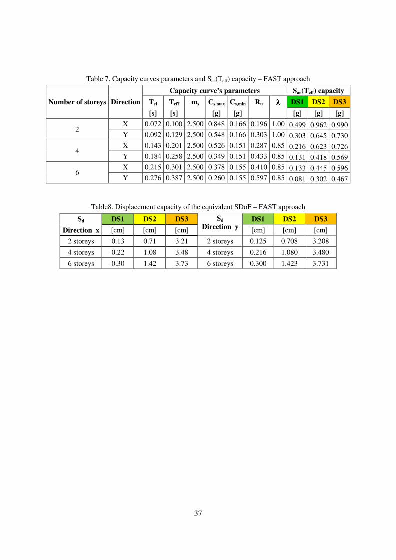
37

Table 7. Capacity curves parameters and Sae(Teff) capacity – FAST approach

Number of storeys Direction

Capacity curve’s parameters Sae(Teff) capacity

Tel Teff ms Cs,max Cs,min Ru λλλλ DS1 DS2 DS3

[s] [s]

[g] [g]

[g] [g] [g]

2 X 0.072 0.100 2.500 0.848 0.166 0.196 1.00 0.499 0.962 0.990

Y 0.092 0.129 2.500 0.548 0.166 0.303 1.00 0.303 0.645 0.730

4 X 0.143 0.201 2.500 0.526 0.151 0.287 0.85 0.216 0.623 0.726

Y 0.184 0.258 2.500 0.349 0.151 0.433 0.85 0.131 0.418 0.569

6 X 0.215 0.301 2.500 0.378 0.155 0.410 0.85 0.133 0.445 0.596

Y 0.276 0.387 2.500 0.260 0.155 0.597 0.85 0.081 0.302 0.467

Table8. Displacement capacity of the equivalent SDoF – FAST approach

Sd DS1 DS2 DS3 Sd

Direction y DS1 DS2 DS3

Direction x [cm] [cm] [cm] [cm] [cm] [cm]

2 storeys 0.13 0.71 3.21 2 storeys 0.125 0.708 3.208

4 storeys 0.22 1.08 3.48 4 storeys 0.216 1.080 3.480

6 storeys 0.30 1.42 3.73 6 storeys 0.300 1.423 3.731

38

7 COMPARATIVE DAMAGE ASSESSMENT

The results of the three different vulnerability approaches described allow a final comparison in

terms of capacity curves and IN2 curves. On the other hand, notwithstanding the significance of the

latter direct comparison, the final test-bed of each methodology is the evaluation of DS thresholds

in terms of spectral displacements and PGA.

Figure 14 compare the capacity curves and the IN2 curves in terms of Sa(Teff), while Figure 14

provides a similar comparison in terms of PGA. The scaling procedure of the IN2 ordinate is made

according the same criterion for the three methods. In fact, the ratio between the spectral

acceleration at Teff and the PGA on rigid soil type of the spectrum considered represents the scaling

factor that resizes the ordinates of the IN2 curves; thus, it allows switching from Sa(Teff) to PGA. In

Figure 14 and 15 the threshold of the three DS considered are also shown for the three vulnerability

methods.

In Table 9, damage threshold in terms of PGA on rigid soil (A soil class) are shown for the three

methodologies considered. Given the fact that the constant shape spectra of Eurocode 8 is

characterized by a fixed soil amplification factor S; equal to 1.2, 1.15, 1.35, and 1.4, respectively for

soil types B to E; the PGA values in Table 9 can be easily scaled aimed at accounting for the effect

of soil amplification on damage thresholds.

Table 9. Comparison between PGA capacities

Number of storeys Direction

PGA DAMAGE STATE

EXACT POST FAST

DS1 DS2 DS3 DS1 DS2 DS3 DS1 DS2 DS3

[g] [g] [g] [g] [g] [g] [g] [g] [g]

2 X 0.226 0.427 0.459 0.254 0.420 0.447 0.211 0.407 0.419

Y 0.115 0.235 0.287 0.140 0.245 0.295 0.114 0.243 0.275

4 X 0.083 0.199 0.250 0.106 0.196 0.236 0.064 0.185 0.215

Y 0.046 0.122 0.161 0.064 0.131 0.191 0.039 0.124 0.168

6 X 0.052 0.137 0.205 0.073 0.150 0.186 0.039 0.132 0.177

Y 0.032 0.083 0.114 0.047 0.105 0.155 0.024 0.089 0.138

Relative errors between the three vulnerability methodologies are shown in Table 10 and 11,

respectively for damage thresholds in terms of PGA and spectral displacements. Relative errors of

EXACT with respect to POST approach are shown on the right, while, on the left, the relative errors

of FAST with respect to POST are shown.

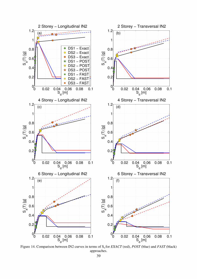
39


Sd [m]

Sa(T

) [g

]

(a)

0 0.02 0.04 0.06 0.08 0.10

0.2

0.4

0.6

0.8

1

1.2

DS1 − ExactDS2 − ExactDS3 − ExactDS1 − POSTDS2 − POSTDS3 − POSTDS1 − FASTDS2 − FASTDS3 − FAST


Sd [m]

Sa(T

) [g

]

(b)

0 0.02 0.04 0.06 0.08 0.10

0.2

0.4

0.6

0.8

1

1.2


Sd [m]

Sa(T

) [g

]

(c)

0 0.02 0.04 0.06 0.08 0.10

0.2

0.4

0.6

0.8

1

1.2


Sd [m]

Sa(T

) [g

](d)

0 0.02 0.04 0.06 0.08 0.10

0.2

0.4

0.6

0.8

1

1.2


Sd [m]

Sa(T

) [g

]

(e)

0 0.02 0.04 0.06 0.08 0.10

0.2

0.4

0.6

0.8

1

1.2


Sd [m]

Sa(T

) [g

]

(f)

0 0.02 0.04 0.06 0.08 0.10

0.2

0.4

0.6

0.8

1

1.2

Figure 14. Comparison between IN2 curves in terms of Sa for EXACT (red), POST (blue) and FAST (black)

approaches.

40


Sd [m]

PG

A [g]

(a)

0 0.02 0.04 0.06 0.08 0.10

0.1

0.2

0.3

0.4

0.5

DS1 − ExactDS2 − ExactDS3 − ExactDS1 − POSTDS2 − POSTDS3 − POSTDS1 − FASTDS2 − FASTDS3 − FAST


Sd [m]

PG

A [g]

(b)

0 0.02 0.04 0.06 0.08 0.10

0.1

0.2

0.3

0.4

0.5


Sd [m]

PG

A [

g]

(c)

0 0.02 0.04 0.06 0.08 0.10

0.1

0.2

0.3

0.4

0.5


Sd [m]

PG

A [

g]

(d)

0 0.02 0.04 0.06 0.08 0.10

0.1

0.2

0.3

0.4

0.5


Sd [m]

PG

A [g]

(e)

0 0.02 0.04 0.06 0.08 0.10

0.1

0.2

0.3

0.4

0.5


Sd [m]

PG

A [

g]

(f)

0 0.02 0.04 0.06 0.08 0.10

0.1

0.2

0.3

0.4

0.5

Figure 15 Comparison between IN2 curves in terms of PGA for EXACT (red), POST (blue) and FAST

(black) approaches.

41

Table 10. Errors referred to PGA capacity

Number

of storeys Direction

PGA

EXACT POST

POST

e − PGA

FAST POST

POST

e −

DS1 DS2 DS3 DS1 DS2 DS3

2 X -0.112 0.018 0.027 -0.171 -0.032 -0.064

Y -0.177 -0.040 -0.027 -0.182 -0.008 -0.067

4 X -0.222 0.012 0.059 -0.399 -0.060 -0.089

Y -0.289 -0.075 -0.156 -0.395 -0.058 -0.117

6 X -0.284 -0.089 0.103 -0.456 -0.122 -0.049

Y -0.314 -0.210 -0.267 -0.485 -0.146 -0.110

Table 11. Errors referred to displacement capacity of the equivalent SDoF

Number

of

storeys

Direction

| iSd DS

EXACT POST

POST

e − | iSd DS

FAST POST

POST

e −

DS1 DS2 DS3 DS1 DS2 DS3

2 X -0.166 -0.144 -0.177 0.064 0.044 -0.165

Y -0.141 -0.113 -0.168 0.063 0.040 -0.166

4 X -0.194 -0.027 -0.191 0.102 0.033 -0.115

Y -0.152 -0.024 -0.018 0.090 -0.042 -0.137

6 X -0.200 -0.202 -0.154 0.067 -0.099 -0.101

Y -0.102 -0.218 -0.188 0.043 -0.102 -0.107

The observation of the IN2 curves in terms of Sa(Teff) in Figure 14 shows how the FAST

approach is always conservative respect to both POST and EXACT approach. The explanation of the

latter observation can be found in the differences between the curves that, in turn, correspond to the

different hypotheses of each methodology:

• Elastic and effective periods evaluated according each methodology are similar to each

other.

• The three approaches, excluding the two storey case, have similar values of Cs,max, which is

mostly defined by infill contribution. It confirms the reliability of Equation (16) in which α

was considered equal to 0.5. In the case of two storeys building the approximate evaluation

of α is evidently underestimated.

• The value of ductility s

µ evaluated in the EXACT and POST approaches is generally higher

with respect to the value (equal to 2.5) assumed in the case of FAST approach. The latter

result leads to a lower slope of the second branch of the IN2 curve according to FAST

method, as it can be seen in Figure 14.

42

• The simplified simulated design procedure adopted in the FAST approach seems to lead to a

value of Cs,min generally lower with respect to the more accurate simulated design

approaches in the POST and EXACT. Such results, given the R-µ-T relationship employed

leads to lower slope of the third branch of the IN2 curve.

• The highest relative errors between large scale methodologies, POST and FAST, versus the

detailed EXACT approach are observed in the case of the six storey building. The latter is

the result of single storey plastic mechanism made in both the large scale approaches. In

particular, according to the detailed assessment in the EXACT approach the plastic

mechanism involves more than one storey; thus, in the longitudinal direction a highest

value of Cs,min and a lower value of Cs,max can be observed in EXACT results.

Differences in the IN2 curves plotted in terms of Sa(T) are not affected by the homothetic

scaling procedure that leads to the IN2 curves in terms of PGA on rigid soil (see Figure 15).

Furthermore, in Table 10 the comparison between the three methods is provided in terms of

characteristic displacements of the three damage states considered. It is worth to note that the

general trends of the relative errors are acceptable. It is interesting to observe that the POST

approach leads, respect to the EXACT approach DS displacements always higher, notwithstanding

the shear-type hypothesis adopted in the first method that would conceptually lead to lower

displacements. The latter result can be explained by the different value of the first mode participant

factors (1

Γ ) considered in the two methods, lower in the case of the POST approach. Conversely,

the FAST approach leads to higher displacement values with respect to the POST in the case of

DS1, while to lower displacements with respect to the POST in the case of DS3 for the all three

benchmark structures considered.

The results of the three approaches described in this study can be finally summarized by the

comparisons in terms of PGA capacities at the three different DS considered, as shown in Table 11.

The relative errors can be considered acceptable. The POST is generally non conservative with

respect to the EXACT results, especially if the DS1 is considered. The FAST approach is always

conservative with respect to the POST. It is worth to note that the significant differences in terms of

PGA for DS1 are clearly a result of the procedure to increase the accuracy in the elastic branch of

the IN2 curve employed in the case of the EXACT and POST approach. Such increase in the

accuracy was not employed in the FAST approach given its intrinsically approximate nature that

does not fit with the more accurate procedure suggested in Dolsek and Fajfar (2005).

It should be emphasized how the approximate procedure in general, and in particular the FAST

method, lead to results that are comparable to the results of the EXACT detailed approach;

43

especially if the poor quality of the information and low computational efforts required are

considered.

Finally, the results obtained through the three vulnerability approaches in terms of PGA are

compared with the shake map of the 20th

of May mainshock according to INGV (see Figure 16).

First of all it should be highlighted that the damage thresholds in terms of PGA shown in Table 9

are computed for the case of rigid soil (A soil class) and for the constant shape spectra according to

EC8 (type 1). Conversely, even if on the basis of very macroscopic geological scale, the most of the

area struck by the earthquake is characterized by D soil class. The latter aspect is accounted for

considering the D soil amplification factor according to EC8 (equal to 1.35).

By means of a simple amplification of the PGA values in Table 9, PGA thresholds at each

damage state can be estimated for the case of D soil class. In Table 12, for each vulnerability

methodology and each DS, the minimum PGA among the two principal directions of the benchmark

buildings are shown.

The analysis of the data provided by ISTAT (see section 2), aimed at characterizing the building

stock, showed that the area struck by the earthquake was mostly characterized by low to medium

rise buildings (from 2 up to 4 storeys). Hence, the comparisons with the PGA data are referred to

the first two benchmark buildings.

From Table 12 the following information can be extrapolated, considering the mean value

obtained from the three methodologies:

• DS1 is equal to 0.17g for the 2 storey buildings, while to 0.07g for the 4 storey building



The comparison of the numerical PGA thresholds, at the three DSs, and the shake map allows

some preliminary remarks. In particular, such remarks are affected by two basic hypotheses: (i) a

uniform distribution of the RC buildings on the area is assumed, given the lack of disaggregated

data from the ISTAT reference; (ii) the benchmark buildings considered are defined as

representative of the whole building stock.

First of all, it is easy to recognize that numerical results predict a DS3 damage only in the case

of RC buildings localized in the epicentral area. Furthermore, higher buildings are on average

susceptible of more significant damage given the PGA of the earthquake. According to the

numerical data, most of four storeys buildings should be characterized by DS1and DS2 (with the

exception of the only epicentral area).

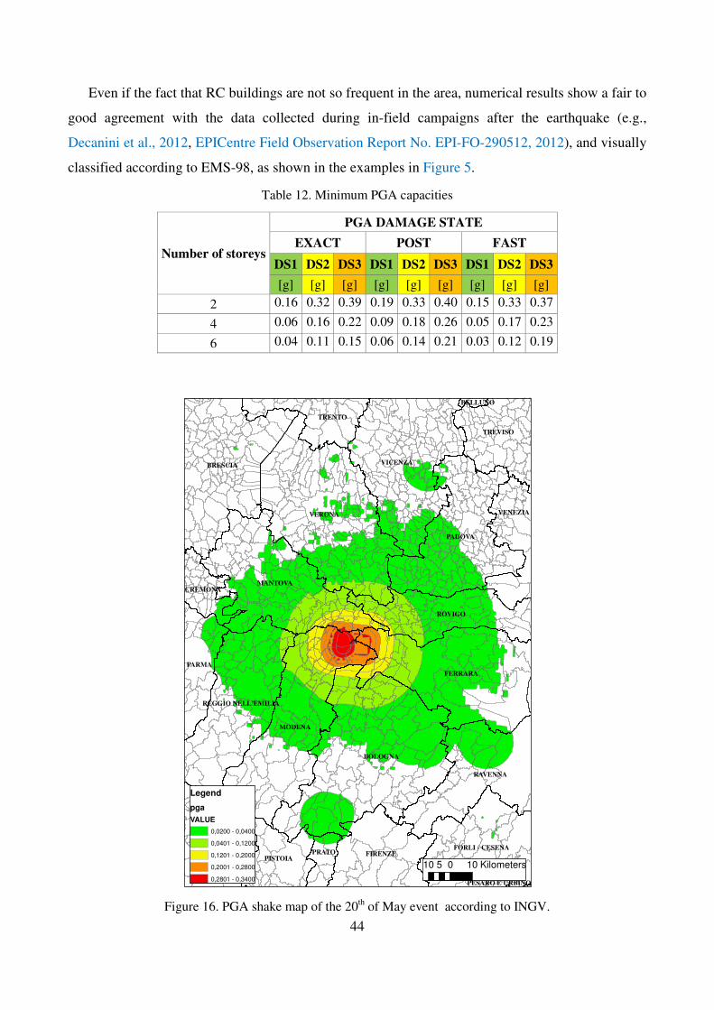
44

Even if the fact that RC buildings are not so frequent in the area, numerical results show a fair to

good agreement with the data collected during in-field campaigns after the earthquake (e.g.,

Decanini et al., 2012, EPICentre Field Observation Report No. EPI-FO-290512, 2012), and visually

classified according to EMS-98, as shown in the examples in Figure 5.

Table 12. Minimum PGA capacities

Number of storeys

PGA DAMAGE STATE

EXACT POST FAST

DS1 DS2 DS3 DS1 DS2 DS3 DS1 DS2 DS3

[g] [g] [g] [g] [g] [g] [g] [g] [g]

2 0.16 0.32 0.39 0.19 0.33 0.40 0.15 0.33 0.37

4 0.06 0.16 0.22 0.09 0.18 0.26 0.05 0.17 0.23

6 0.04 0.11 0.15 0.06 0.14 0.21 0.03 0.12 0.19

^

BOLOGNA

VERONA

MODENA

VICENZA

FERRARA

PADOVA

BRESCIA

MANTOVA

RAVENNA

ROVIGO

LUCCA

FIRENZE

TREVISO

FORLI - CESENA

PARMA

PISTOIA

TRENTO

VENEZIA

PRATO

REGGIO NELL’EMILIA

CREMONA

BELLUNO

PESARO E URBINO

Legend

pga

VALUE

0,0200 - 0,0400

0,0401 - 0,1200

0,1201 - 0,2000

0,2001 - 0,2800

0,2801 - 0,3400

10 0 105 Kilometers

Figure 16. PGA shake map of the 20th of May event according to INGV.

45

8 CONCLUSIONS AND PERSPECTIVES

A three level vulnerability approach for the evaluation of the performances of RC infilled

structures was provided and aimed at looking into the observed performances of RC structures

during the 2012 Emilia earthquake. The vulnerability study was pursued on three benchmark

buildings representative of the building stock of the area struck by the earthquake. The historical

and recent evolution of seismic codes and the seismic classification of the area were considered to

assess the design approach that the benchmark structures considered should have to be

representative of the most common construction practice at the site.

The three damage assessments were pursued on the benchmark structures beginning with a

detailed push-over based methodology, named EXACT. Two large scale vulnerability

methodologies were described and compared in terms of basic hypotheses. The only first three

grades of damage according to EMS-98 scale were considered; since for those three grades a

mechanical and empirical evaluation of the displacement capacities can be carried out on the basis

of the behavior of masonry infills.

Results in terms of spectral displacements, spectral acceleration and PGA characterizing the

three damage states, according to the three methodologies were compared. The two large scale

approaches showed a fair to good agreement with the results of the detailed assessment. Relative

errors are characterized by a conservative general trend that in some way can provide a validation of

the large scale methodologies provided.

Finally a comparison with the registered PGA during the mainshock event of the 2012 Emilia

sequence explains the limited damage observed to RC structures in the area struck by the

earthquake. In fact, in the only epicentral zone, the PGA characterizing moderate structural damage

and vey heavy nonstructural damage (grade 3 according to EMS-98) was exceeded. The study

provided shows the reliability of the large scale approaches also in terms of observed damage.

American Society of Civil Engineers (ASCE), Seismic Rehabilitation of Existing Buildings, ASCE/SEI 41-

06, Reston, Virginia, 2007.

Augenti N., (2009). Un database per l’archiviazione e l’analisi di dati sperimentali relativi alle murature.

Proccedings of the 3rd

conference Wondermasonry - Workshop on design and rehabilitation of masonry

structures, 8 October, Lacco Ameno, Italy.

Bal I.E., Crowley H., Pinho R., Gulay F.G., 2007. Structural characteristics of Turkish RC building stock in

Northern Marmara region for loss assessment applications. ROSE Research Report No. 2007/03, IUSS

Press, Pavia, Italy.

Benavent-Climent A., Akiyama H., Lopez-Almansa F., Pujades L.G. (2004). Prediction of ultimate

earthquake resistance of gravity-load designed RC buildings. Engineering Structures 26, 1103-1113.

46

Bindi D, Pacor F, Luzi L, Puglia R, Massa M, Ameri G, Paolucci R, (2011). Ground motion prediction

equations derived from the Italian strong motion database, Bulletin of Earthquake Engineering, 9(6),

1899-1920.

Biskinis D. and Fardis M. N. (2010a), Deformations at flexural yielding of members with continuous or lap-

spliced bars. Structural Concrete 11(3): 128-138.

Biskinis DE and Fardis MN (2010b) Flexure-controlled ultimate deformations of members with continuous

or lap-spliced bars. Structural Concrete 11(2): 93-108.

Borzi B., Elnashai A. (2000). Refined force reduction factor for seismic design. Engineering Structures 22,

1244-1260.

CEN (2004) Eurocode 8: design of structures for earthquake resistance—Part 1: general rules, seismic

actions and rules for buildings. European Standard EN 1998-1:2003- Comité Européen de Normaliation,

Brussels.

Celarec, D., Ricci, P., Dolšek, M. (2012). The sensitivity of seismic response parameters to the uncertain

modelling variables of masonry-infilled reinforced concrete frames. Engineering Structures, 35, 165-177.

Chioccarelli E, De Luca F, Iervolino I. (2012a), Preliminary study of Emilia (May 20th 2012) earthquake

ground motion records V2.11, [available at http://www.reluis.it].

Chioccarelli, E., F. De Luca and I. Iervolino (2012b). Preliminary study of Emilia (May 29th 2012)

earthquake ground motion records V1.0, [available at http://www.reluis.it].

Chopra A.K., Chintanapakdee C., (2004). Inelastic Deformation Ratios for Design and Evaluation of

Structures: Single-Degree-of-Freedom Bilinear Systems. ASCE Journal of Structural Engineering,

130(9), 1309-1319.

Colangelo F. (2012). A simple model to include fuzziness in the seismic fragility curve and relevant effect

compared with randomness. Earthquake Engineering and Structural Dynamics, 41, 969-986.

Cosenza E., Manfredi G., Polese M., Verderame G.M., (2005). A multilevel approach to the capacity

assessment of existing RC buildings. Journal of Earthquake Engineering, 9(1), 1-22.

CS.LL.PP.; 2009: Istruzioni per l'applicazione delle norme tecniche delle costruzioni. Gazzetta Ufficiale

della Repubblica Italiana, 47.

Decanini L., Liberatore D., Liberatore L., Sorrentino L., (2012). PRELIMINARY REPORT ON THE 2012,

MAY 20TH, EMILIA EARTHQUAKE v1.0, [available at http://www.eqclearinghouse.org/2012-05-20-

italy-it/files/2012/06/Emilia2012_DecaniniLiberatoreLiberatoreSorrentino_v1.pdf].

Decreto Ministeriale del 16/1/1996 (1996) Norme tecniche per le costruzioni in zone sismiche.Gazzetta

Ufficiale della Repubblica Italiana, 29 del 5/2/1996 (in Italian)

Decreto Ministeriale del 14 Gennaio 2008: Norme tecniche per le costruzioni. Gazzetta Ufficiale della

Repubblica Italiana, 29. 4/2/2008 (in Italian).

Decreto Ministeriale n. 40 del 3/3/1975 (1975) Approvazione delle norme tecniche per le costruzioni in zone

sismiche. Gazzetta Ufficiale della Repubblica Italiana, 93 dell’8/4/1975 (in Italian)

De Luca F., 2011. Records, capacity curve fits and reinforced concrete damage states within a performance

based earthquake engineering framework. PhD thesis. Department of Structural Engineering, University

of Naples Federico II. Advisors: G. Manfredi, I. Iervolino, G.M. Verderame. Available at

http://wpage.unina.it/flavia.deluca/.

47

De Luca F., Verderame G.M., Gomez-Martinez F., Perez-Garcia A., (2012). The structural role played by

masonry infills on RC building performances after the 2011 Lorca, Spain, earthquake. Bulletin of

Earthquake Enginerring, (under review).

De Marco R., Marsan P. (Eds.), (1986). Atlante della classificazione sismica del territorio nazionale, Servizio

Sismico del Consiglio Superiore dei Lavori Pubblici, Istituto Poligrafico e Zecca dello Stato Italiano,

Roma.

Dolce M., Cardone D., Ponzo F.C., Valente C., (2005). Shaking table tests on reinforced concrete frames

without and with passive control systems. Earthquake Engineering and Structural Dynamics, 34, 1687-

1717.

Dolšek, M., Fajfar, P. (2004a). Inelastic spectra for infilled reinforced concrete frames. Earthquake

Engineering and Structural Dynamics, 33(15), 1395-1416.

Dolšek, M., Fajfar, P. (2004b). IN2 - A simple alternative for IDA. Proceedings of the 13th World

Conference on Earthquake Engineering, Vancouver, B.C., Canada, August 1-6. Paper No. 3353.

Dolšek, M., Fajfar, P. (2005). Simplified non-linear seismic analysis of infilled reinforced concrete

frames.Earthquake Engineering and Structural Dynamics, 34(1), 49-66.

Dolšek, M., Fajfar, P. (2008). The effect of masonry infills on the seismic response of a four-storey

reinforced concrete frame – a deterministic assessment. Engineering Structures, 30(7), 1991-2001.

EPICentre Field Observation Report No. EPI-FO-200512 (2012), The 20th May 2012 EmiliaRomagna

Earthquake, [available at http://www.ucl.ac.uk/~ucestor/research-earthquake/EPICentre_Report_EPI-

FO-200512-v2.pdf ].

EPICentre Field Observation Report No. EPI-FO-290512 (2012), The 29th May 2012 EmiliaRomagna

Earthquake, [available at http://www.ucl.ac.uk/~ucestor/research-earthquake/EPICentre_Report_EPI-

FO-290512.pdf].

Fardis, M.N. (2007). LESSLOSS – Risk mitigation for earthquakes and landslides. Guidelines for

displacement based design of buildings and bridges. Report No. 5/2007, IUSS Press, Pavia, Italy.

Galasso C., Cosenza E., Maddaloni G. (2011). Statistical analysis of reinforcing steel properties for seismic

design of RC structures. Proceedings of the 14th European Conference on Earthquake Engineering,

August 30-September 3, Ohrid, Republic of Macedonia.

Giovinazzi S., 2005. The vulnerability assessment and the damage scenario in seismic risk analysis. PhD

Thesis, Technical University Carolo-Wilhelmina at Braunschweig, Braunschweig, Germany and

University of Florence, Florence, Italy.

Giovinazzi S., Lagomarsino S., (2004). A macroseismic method for the vulnerability assessment of

buildings. Proceedings of the 13th World Conference on Earthquake Engineering, Vancouver, Canada,

August 1-6. Paper No. 896.

Gomez-Martinez F., Perez-Garcia A., De Luca F., Verderame G.M., Manfredi G., (2012). Preliminary study

of the structural role played by masonry infills on RC building performances after the 2011 Lorca, Spain,

earthquake, Proceedings of the 15th World Conference on Earthquake Engineering, September 24-28,

Lisbon, Portugal.

Goretti A.. and Di Pasquale G., (2006). Technical emergency management. In: Oliveira C.S., Roca A., and

Goula X. Editors; Assessing and managing earthquake risk, Springer, chapter 16.

48

Iervolino, I. (2012). Probabilità e salti mortali: le insidie della validazione dell’analisi di pericolosità

attraverso l’occorrenza di singoli terremoti. Progettazione Sismica. IUSS Press, Pavia, Italy. (in Italian,

in press).

Iervolino I., Manfredi G., Polese M., Verderame G.M., Fabbrocino G., (2007). Seismic risk of R.C. building

classes. Engineering Structures, 29(5), 813-820.

Iervolino I., De Luca F., Chioccarelli E., (2012). Peak and cyclic, elastic and inelastic, engineering seismic

demand in the 2012 Emilia sequence: preliminary analysis, Annals of Geophysics, (under review).

Lai C, Foti S, Rota M, (2009). Input sismico e stabilità geotecnica dei siti in costruzione. IUSS Press, Pavia,

Italy.

Mainstone R.J., 1971. On the stiffnesses and strengths of infilled frames. Proceedings of the Institution of

Civil Engineering, Supplement IV, 57-90.

Manfredi G., Ricci P., Verderame G.M. (2012), Influence of Infill Panels and Their Distribution on Seismic

Behavior of Existing Reinforced Concrete Buildings, The Open Construction and Building Technology

Journal, 2012, 6, (Suppl 1-M1).

McKenna, F., Fenves, G.L., Scott, M.H. (2004). OpenSees: Open System for Earthquake Engineering

Simulation. Pacific Earthquake Engineering Research Center. University of California, Berkeley, CA,

USA. http://opensees.berkeley.edu.

Ordinanza del Presidente del Consiglio dei Ministri n. 3274 del 20/3/2003 (2003) Primi elementi in materia

di criteri generali per la classificazione sismica del territorio nazionale e di normative tecniche per le

costruzioni in zona sismica. G.U. n. 105 dell’8/5/2003 (in Italian).

Panagiotakos, T.B., Fardis, M.N. (1996). Seismic response of infilled RC frames structures. 11th

WorldConference on Earthquake Engineering, Acapulco, México, June 23-28. Paper No. 225.

Pecce M, Polese M, Verderame GM. Seismic vulnerability aspects of RC buildings in Benevento. In: Pecce

M, Manfredi G, Zollo A. editors. The many facets of seismic risk CRdC AMRA; 2004.

Regio Decreto Legge n. 2229 del 16/11/1939. Norme per la esecuzione delle opere in conglomerate

cementizio semplice od armato. G.U. n. 92 del 18/04/1940. (in Italian).

Ricci, P. (2010). Seismic vulnerability of existing RC buildings. Ph.D. Thesis. University of Naples Federico

II, Naples, Italy.

Ricci, P., De Luca, F., Verderame, G.M. (2011a). 6th April 2009 L’Aquila earthquake, Italy – Reinforced

concrete building performance. Bulletin of Earthquake Engineering 9(1),285-305.

Ricci, P., Verderame G.M., Manfredi G., (2011b) Analytical investigation of elastic period of infilled RC

MRF buildings, Engineering Structures 33(2), 308-319.

Ricci P., De Risi M.T., Verderame G.M., Manfredi G., (2012). Influence of infill distribution and design

typology on seismic performance of low- and mid-rise RC building. Bulletin of Earthquake Engineering,

(under review).

Rossetto T., Elnashai A., (2005). A new analytical procedure for the derivation of displacement-based

vulnerability curves for populations of RC structures. Engineering Structures, 7(3), 397-409.

STIL, software, (2012) Verderame G.M., Ricci P., Esposito E., Manfredi G. Available at www.reluis.it.

49

Stucchi M, Meletti C, Montaldo V, Crowley H, Calvi GM, Boschi E. Seismic Hazard Assessment (2003-

2009) for the Italian Building Code, Bulletin of the Seismological Society of America 2011;

101(4):1885-1911.

Verderame GM, Stella A., Cosenza E., (2001). Le proprietà meccaniche degli acciai impiegati nelle strutture

in c.a. realizzate negli anni 60’. X Convegno nazionale “L’Ingegneria Sismica in Italia”, Potenza-Matera,

9-13 September.

Verderame G.M., Polese M., Mariniello C., Manfredi G., (2010a). A simulated design procedure for the

assessment of seismic capacity of existing reinforced concrete buildings, Advances in Engineering

Software, 41, 323–335.

Verderame, G.M., Ricci, P., Manfredi, G., Cosenza, E. (2010b). Ultimate chord rotation of RC columns with

smooth bars: some considerations about EC8 prescriptions. Bulletin of Earthquake Engineering,

8(6),1351-1373.

A THREE LEVEL VULNERABILITY APPROACH FOR THE DAMAGE ... · A THREE LEVEL VULNERABILITY APPROACH FOR...

Documents

Transcript of A THREE LEVEL VULNERABILITY APPROACH FOR THE DAMAGE ... · A THREE LEVEL VULNERABILITY APPROACH FOR...