A three-dimensional ray-driven attenuation, scatter and...

This content has been downloaded from IOPscience. Please scroll down to see the full text.

Download details:

IP Address: 155.98.164.39

This content was downloaded on 22/05/2015 at 22:28

Please note that terms and conditions apply.

A three-dimensional ray-driven attenuation, scatter and geometric response correction

technique for SPECT in inhomogeneous media

View the table of contents for this issue, or go to the journal homepage for more

2000 Phys. Med. Biol. 45 3459

(http://iopscience.iop.org/0031-9155/45/11/325)

Home Search Collections Journals About Contact us My IOPscience

iopscience.iop.org/page/terms

http://iopscience.iop.org/0031-9155/45/11

http://iopscience.iop.org/0031-9155

http://iopscience.iop.org/

http://iopscience.iop.org/search

http://iopscience.iop.org/collections

http://iopscience.iop.org/journals

http://iopscience.iop.org/page/aboutioppublishing

http://iopscience.iop.org/contact

http://iopscience.iop.org/myiopscience

Phys. Med. Biol. 45 (2000) 3459–3480. Printed in the UK PII: S0031-9155(00)12838-6

A three-dimensional ray-driven attenuation, scatter andgeometric response correction technique for SPECT ininhomogeneous media

I Laurette†§, G L Zeng†, A Welch‡, P E Christian† and G T Gullberg†† Department of Radiology, University of Utah, Salt Lake City, Utah 84108-121, USA‡ Department of Biomedical Physics and Bioengineering, University of Aberdeen, AberdeenAB25 2ZD, Scotland, UK

Received 24 March 2000, in final form 4 July 2000

Abstract. The qualitative and quantitative accuracy of SPECT images is degraded by physicalfactors of attenuation, Compton scatter and spatially varying collimator geometric response.

This paper presents a 3D ray-tracing technique for modelling attenuation, scatter andgeometric response for SPECT imaging in an inhomogeneous attenuating medium. Themodel is incorporated into a three-dimensional projector–backprojector and used with themaximum-likelihood expectation-maximization algorithm for reconstruction of parallel-beam data.A transmission map is used to define the inhomogeneous attenuating and scattering object beingimaged. The attenuation map defines the probability of photon attenuation between the source andthe scattering site, the scattering angle at the scattering site and the probability of attenuation ofthe scattered photon between the scattering site and the detector. The probability of a photon beingscattered through a given angle and being detected in the emission energy window is approximatedusing a Gaussian function. The parameters of this Gaussian function are determined using physicalmeasurements of parallel-beam scatter line spread functions from a non-uniformly attenuatingphantom. The 3D ray-tracing scatter projector–backprojector produces the scatter and primarycomponents. Then, a 3D ray-tracing projector–backprojector is used to model the geometricresponse of the collimator.

From Monte Carlo and physical phantom experiments, it is shown that the best results areobtained by simultaneously correcting attenuation, scatter and geometric response, compared withresults obtained with only one or two of the three corrections. It is also shown that a 3D scattermodel is more accurate than a 2D model.

A transmission map is useful for obtaining measurements of attenuation and scatter in SPECTdata, which can be used together with a model of the geometric response of the collimator to obtaincorrected images with quantitative and diagnostically accurate information.

1. Introduction

Accuracy of SPECT images is degraded by physical effects of attenuation, Compton scatter,detector response and patient movement. Compensation for attenuation (Tsui et al 1989) hasbeen studied at great length, and several methods have been proposed. However, correcting forattenuation only is not sufficient because the erroneous information given by scattered photonstends to produce an over-compensation. This is seen as the major source of apparent over-correction in the inferior wall of the left ventricle of the heart, which is associated with hepaticuptake (King et al 1996). Consequently, it is necessary to correct simultaneously for attenuation

§ Present address: Faculte de Medecine, Universite de Nice-Sophia Antipolis, 28 Avenue de Valombrose, 06107Nice Cedex 2, France.

0031-9155/00/113459+22$30.00 © 2000 IOP Publishing Ltd 3459

3460 I Laurette et al

and scatter. It has been shown that when accurate scatter models are used the over-correction inthe heart is improved (Tsui et al 1994) and the signal to noise ratio (SNR) of small cold lesionsis also improved (Beekman et al 1996, 1997a, Hutton et al 1996, Hutton 1997). In addition, ithas been known for some time that the geometric response of the collimator produces a spatiallyvarying partial volume effect in SPECT images. It was found, for example in dynamic cardiacSPECT (Gullberg et al 1998), that the correction for geometric response improves the partialvolume effect and reduces the bias in estimated kinetic parameters (Kadrmas et al 1999). Whilesome methods perform presubtraction of the scatter component from projection data before thereconstruction process, linear algebraic methods allow the incorporation of attenuation, scatterand geometric response corrections in the reconstruction process. This is done by utilizing theprojector–backprojector (transition matrix) which models the acquisition process in order toproduce improved qualitative and quantitative SPECT images.

A class of widely used and widely studied scatter compensation methods is based onthe estimation of the scattered component in the photopeak projection data and subsequentsubtraction or deconvolution of the scatter contribution from the measured projection data.Many of the subtraction-based scatter compensation methods use multiple energy windowacquisition methods (DeVito et al 1989, Frey et al 1992, Gagnon et al 1989, Halama et al1988, Hamill and DeVito 1989, Jaszczak et al 1984, 1985, King et al 1992, Koral et al 1988,1990, Lowry and Cooper 1987, Ogawa et al 1991) to estimate the scatter contribution. Theestimated scatter component can be subtracted from the photopeak projection data to obtain theprimary projection data. Then SPECT reconstruction methods without scatter compensationcan be used. Scatter compensation methods in this class are fast and simple but increase thenoise in the reconstructed images. The deconvolution methods use kernels that are obtainedfrom physical measurements using a gamma-camera (Axelsson et al 1984, Floyd et al 1985b,Meikle et al 1994, Msaki et al 1987, 1989). Usually, the scatter component is deconvolvedfrom the projection data before reconstruction. Deconvolution or restoration filtering methodscan also be used to correct for geometric response. The restoration filtering is implemented in afiltered backprojection algorithm (Gilland et al 1988, King et al 1983, 1984, Ogawa et al 1988)where the blurring is approximated by a spatially invariant blurring function. Another approachuses the frequency–distance principle (Elmbt and Walrand 1993, Glick et al 1994, Lewitt et al1989, Xia et al 1995) which incorporates the distance-dependent collimator blurring into theFourier transform of the sinogram.

Another class of scatter and geometric response compensation methods is based onmodelling the scatter and collimator geometric effects (the scatter and geometric responsefunction) in the projector–backprojector used in linear algebraic methods (Beekman et al1993, 1996, Floyd et al 1985b, Frey and Tsui 1993, Frey et al 1993, Welch et al 1995). It hasbeen shown that a realistic projector–backprojector enables accurate compensation for non-uniform attenuation (Tsui et al 1989), detector response (Formiconi et al 1989, Gilland et al1994, Tsui et al 1988, Tsui and Gullberg 1990, Zeng et al 1991), and scatter (Bai et al 2000,Beekman et al 1993, 1994, 1996, 1997b, Beekman and Viergever 1995, Bowsher and Floyd1991, Cao et al 1994, Floyd et al 1986, 1987, 1989, Frey and Tsui 1993, 1994, 1996, Frey et al1993, Hutton et al 1996, Hutton 1997, Ju et al 1995, Kadrmas et al 1996, 1997, 1998, Meikleet al 1994, Riauka et al 1996, Veklerov et al 1988, Walrand et al 1994, Welch et al 1995, Wellset al 1997). The accuracy of a linear algebraic scatter and geometric compensation methoddepends upon the accuracy of the model used. A complicating factor in modelling scatter isthat the scatter response is generally different for every point in the object to be imaged andcannot easily be calculated analytically from geometric formulations as can be done for thegeometric response (Tsui et al 1988, Zeng et al 1991), which can be calculated from formulaebased upon the shape and size of the collimator hole (Tsui and Gullberg 1990).

Correction technique for SPECT 3461

Several techniques have been developed for calculating the transition matrix (for scatterand geometric response modelling) so that it is a function of the collimator geometry and theanatomy being imaged:

(a) One technique computes the transition matrix using Monte Carlo (MC) simulations(Bowsher and Floyd 1991, Floyd et al 1985a, 1986, 1987, 1989, Frey and Tsui 1990,Veklerov et al 1988). This approach requires large data storage capacities and longcomputation times.

(b) A second technique takes actual physical measurements (Beekman et al 1994, Formiconiet al 1989, Walrand et al 1994).

(c) Another technique is referred to as slab-derived scatter estimation. This technique firstcalculates and stores the scatter response tables for a point source behind slabs of a rangeof thicknesses, and then tunes the model to various object shapes (Beekman et al 1993,1996, 1997b, Beekman and Viergever 1995, Frey and Tsui 1993, Frey et al 1993). A tablethat occupies only a few megabytes of memory is sufficient to represent this scatter modelfor fully 3D reconstruction.

(d) Another method is based upon the integration of the Klein–Nishina formula in non-uniformmedia (Cao et al 1994, Riauka and Gortel 1994, Riauka et al 1996, Wells et al 1998).Like Monte Carlo techniques, this technique requires large data storage capacities andlong computation times.

(e) Another approach, which improves computation and storage requirement, uses an incre-mental blurring approach to model the scatter and geometric response (Bai et al 1998,2000, Zeng et al 1998, 1999). This approach is an extension of a method that wasoriginally implemented for uniform attenuators by producing an effective scatter sourceestimation (ESSE) where the activity image is convolved with several convolution kernelsto obtain the ESSE (Frey and Tsui 1996, Kadrmas et al 1998). The ESSE is estimatedby forward projection using a projector that models both attenuation and geometric de-tector response effects. The method models the non-uniform attenuation effect from thescattering point to the detector, but does not model the non-uniform attenuation from thesource to the scattering point. The incremental blurring approach (Bai et al 2000) uses theKlein–Nishina formula to calculate the first-order Compton scatter and an effective scattersource image (ESSI) is obtained using a slice-by-slice blurring model, with the blurringkernels approximated from a transformed Klein–Nishina formula. Scatter projectionscan be obtained by forward-projecting the ESSI using an incremental blurring projector(Bai et al 1998, Zeng et al 1998), which models non-uniform attenuation and geometricdetector response effects.

Most linear algebraic scatter and geometric response compensation methods are imagespace reconstruction methods. It is assumed that the continuous activity distribution is digitizedas a pixel or voxel representation. Ray-driven and pixel-driven projector–backprojectorsthat model the scatter and geometric response are implemented to form the projection andbackprojection images. Using the projection as an example, a pixel-driven projection isperformed as the indexing is accomplished sequentially through the pixel array: first bysearching the nearest projection bin to the projection of the centre of a given pixel; secondby summing to this projection bin the concentration value of the pixel times the point spreadfunction (PSF) of the imaging system. On the contrary, a ray-driven projection cycles throughthe image array along projection rays driven from the detector. For a given bin, the projectionvalue is computed by accumulating the concentration value of each pixel belonging to the raytimes the PSF. In the ray-driven models the geometric response can be approximated by a fan(Tsui et al 1988), or a cone (Zeng et al 1991) of rays emanating from the projection bin with


each ray weighted to match the geometric response of the collimator. The technique we areproposing also uses rays to model the geometric response; however, we have extended theapproach to the modelling of the scatter response. Even though most scatter and geometricresponse compensation methods are image space reconstruction methods, a few publicationshave proposed projection space reconstruction methods to correct for the effects of attenuation(Gullberg et al 1996) and geometric response (Hsieh et al 1998).

The work here is an extension to 3D of the work of Welch et al (1995). The previous 2Dmodel was far from exact since the origin of detected scatter events cannot be restricted to onlya plane but can originate from anywhere throughout the entire volume of the patient’s body.Other models have already been developed that can provide very accurate three-dimensional(3D) scatter compensation in SPECT (Beekman et al 1993, 1996, Ju et al 1995, Frey andTsui 1996, Frey et al 1993). However, their major drawbacks are that their application islimited to homogeneous media and to a specific acquisition geometry. The method presentedin this paper models the distribution of scattered events in the emission projection databy using a variable attenuation map to estimate first-order scatter at each image site byprojecting and backprojecting along all possible lines of scatter using a ray-driven projector–backprojector. The 3D geometric response (detector response) is also modelled using theray-driven projector–backprojector in the work of Zeng et al (1991). The computations in theray-tracing method are based on the method presented in Gullberg et al (1989). The methodhas been tested on a numerical simulation and two sets of phantom data, acquired with a two-detector camera equipped with parallel collimators. The results presented are compared withresults obtained with various combinations of no correction, attenuation correction, geometricresponse correction and scatter correction.

2. Theory

For this section, integral equations are used to describe the model used. In section 3, discreteequations will be used, corresponding to the discretization of the equations developed in thepresent section.

2.1. Attenuation

The photon attenuation from an emission point e to a detection point d is often modelled bythe following equation:

A(e, d) = exp

(−

∫ d

e

M(x) dx

)(1)

where M is the attenuation distribution.

2.2. Three-dimensional Compton scatter model

The detection probability of photons originating from emission point e, scattered at multiplescatter points si , and detected at point d , can be modelled as the complete attenuated path frome to d (including deviations due to scatter), multiplied by the probability of scatter at eachscattering site.

In practice, the method developed must describe as precisely as possible the path of aphoton emitted from a given emission point and received by the detection point, including oneor several deviations due to scatter. Since at least 80% of the scattered events detected in a99mTc study are the result of a single Compton interaction (Floyd et al 1984), we restrict themodel to first-order scatter. Therefore, the detection probability of a photon depends first on


Figure 1. Modelling of the projection including attenuation, scatter and geometric point response.A photon starting from an emission point e (or ray I ), scattered at point s, is detected at point d.The different planes represent different possible scattering angles in 3D. The cone of rays near thedetection point d represents the angles of acceptance of the collimator hole.

the attenuation along the path: from source point to scatter point, and from scatter point todetection point (see figure 1).

Theoretically, scatter probability is the combination of the Klein–Nishina formula with theenergy-dependent detection probability function of the gamma-camera. Rather than attemptto accurately model the distribution of first-order scatter, we decided to use the product of asimple analytical function to evaluate the scatter probability through a given scattering angleand the attenuation coefficient at the scattering site (Welch et al 1995).

Consequently, the number of photons, emitted from point e, scattered at site s, and detectedat point d , is defined by:

Ps(e, s, d) = F(e)A(e, s)�(φ)M(s)A(s, d) (2)

where F is the radionuclide distribution and �(φ) is the scattering probability functiondepending on the scattering angle, φ, defined by the ray from e to s, and the ray from s

to d (see figure 1).This equation can be explained as follows:

(a) A number of photons F(e) are emitted from e.(b) These photons undergo an attenuation factor A(e, s) from the emission source point to

the scattering point.(c) Their scatter probability is expressed by �(φ)M(s).(d) They ultimately undergo a final attenuation factor A(s, d) from the scattering point to the

point of detection.

2.3. Geometric point response

The geometric point response function is the photon fluence distribution on the detector facedetermined by the geometrical aperture of the collimator hole. In the following, the geometricpoint response is derived by considering one collimator hole.


Figure 2. Collimator photon fluence. F is the focal length, Z the distance from the point sourceto the detector plane, L the thickness of the collimator and B is the distance from the back of thecollimator to the front of the detector.

For a point source located at a distance Z from the detector plane (see figure 2), anexpression for the geometric point response in terms of the autocorrelation of the collimatoraperture function α for one collimator hole on the front plane of the collimator can be givenby (Tsui and Gullberg 1990, Metz et al 1980):

G(rT ) =∫ +∞

−∞

∫ +∞

−∞α(σ)α(σ + rT ) dσ (3)

where rT is a function of r , r0 the perpendicular projection of the point source on the detectionplane, and Z (see equation (5)). Both σ and rT are on the σ -plane, which is obtained througha coordinate transformation from the r-plane (Tsui and Gullberg 1990).

In this paper, the collimator aperture function α is assumed to be circular. For a radiusR, the integral in equation (3) can be evaluated by computing the common area of two circles(see figure 2). As described in Zeng et al (1991), equation (3) becomes:

G(rT ) = 2 arccos(∣∣∣ rT

2R

∣∣∣) −∣∣∣ rT2R

∣∣∣√

1 −∣∣∣ rT2R

∣∣∣2. (4)

It can be shown that for parallel geometry the parameter rT in equations (3) and (4) isgiven by (see figure 3):

rT = L

Z(r − r0) (5)

where r is the polar coordinate of detection point d, and r0 is the polar coordinate of the pointsource projection.


Figure 3. Computation of rT for parallel geometry.

In this paper we have focused on parallel geometry, but an analogue model can easily bederived for fan-beam and cone-beam geometry as described in Zeng et al (1991).

Therefore, a projection model of the photons emitted from point e including geometricpoint response can be derived by:

Ppr(e, d) = F(e)G(rT )A(e, d) (6)

where rT depends on the detection point d (equation (5)). This equation describes the modelfor the process of acquiring the primary photons.

2.4. Simultaneous modelling of attenuation, scatter and geometric response

Combining equations (1), (2), and (6), a model of the projection process including attenuation,scatter and geometric response can be described by the following equation (see also figure 1):

Psc(e, s, d) = F(e)A(e, s)︸︷︷︸step 1

�(φ)︸︷︷︸step 2

M(s)︸︷︷︸step 3

A(s, d)︸︷︷︸step 4

G(rT )︸︷︷︸step 5

. (7)

For computation purposes equation (7) is now rewritten for a ray I drawn from scatteringsite s. The number of photons emitted from ray I and detected at point d is equal to:

Psc(I, s, d) =( ∫

I

F (x)A(x, s) dx

)�(φ)M(s)A(s, d)G(rT ). (8)

The integral describes the number of attenuated photons emitted from points of ray I andscattered at site s. The product �(φ)M(v) describes the scatter probability. The last termcorresponds to the projection, including attenuation effect, of the scattered photons onto thedetector point d .

As an approximation, it is considered that scatter is negligible for scattering angles greaterthan π/2. That is to say �(φ) = 0 for φ > π/2. Therefore, integrating over the half-spaceV/2 defined by the scattering point and a plane parallel to the detector (see figure 4), we get:

Psc(s, d) =( ∫

V/2�(φ) dI

∫I

F (x)A(x, s) dx

)M(s)G(rT )A(s, d) (9a)

= Fsc(s)G(rT )A(s, d) (9b)


Figure 4. Scatter estimation is restricted to the points in the volume V/2, defined by the scatteringpoint s and a plane parallel to the detector.

whereFsc can be defined as the scattered radionuclide distribution. Note the similarity betweenequation (6) and equation (9b). Equation (6) models the projection of the radionuclidedistribution, while equation (9b) models the projection of the scattered radionuclidedistribution. In other words, in the first case, the acquisition of primary photons is described,while in the latter case the acquisition of scattered photons is described.

3. Methods

3.1. Reconstruction algorithm

Several studies have developed the idea of using scatter correction only in the projector or ina subtraction scheme (Welch and Gullberg 1998). However, the use of a transition matrix thatincludes all of the corrections for both projection and backprojection steps is theoretically themost appropriate. Therefore, in this study a basic EM algorithm was applied for which aniteration can be written as:

f n+1e = f n

e∑d Red

∑d

(Red

pd∑e′ Re′df

ne′

)(10)

where f is the distribution image to be reconstructed, p represents the projection data and Red

is an element of the transition matrix—including factors for attenuation, scatter and geometricresponse. In this equation, n is the iteration number, e corresponds to the voxel index and d isthe projection bin index.

A voxel and a projection bin are said to be linked if a ray emitted from the bin passesthrough the voxel. The elements Red are derived by discretizing equations (6) and (7) to give

Red =

a(e, d)g(rT ) if e and d are linked

a(e, s)︸︷︷︸step 1

ψ(φ)︸︷︷︸step 2

µ(s)︸︷︷︸step 3

a(s, d)︸︷︷︸step 4

g(rT )︸︷︷︸step 5

otherwise (11)

where a(e, d) = exp(− ∑dx=e µ(x)) is the attenuation factor from voxel e to detection point d.

All the capital letters corresponding to integral equations (6) and (7) have been replaced bysmall letters: µ for M , a for A, g for G, and ψ for �. The first case corresponds to projectionof primary photons only, while the second case describes the effect of scatter.


3.2. Projector/backprojector

The ideal way to solve the system p = Rf would be to store the transition matrix R, thenuse matrix arithmetic to compute equation (10). However, the matrix R is generally too largeto be stored in memory, even if no physical correction is included. The number of non-zeroelements is even larger when geometric response and scatter correction are applied, especiallywhen a 3D model is used, because a projection bin is connected to nearly half of the voxels inthe image (we suppose that the scatter probability is zero when the scatter angle is greater than90◦). Therefore, all the ray-sums are computed directly for each iteration, both for projectionand backprojection, using the algorithm described in (Gullberg et al 1985, 1989).

The algorithm used to compute the projection step is as follows:

loop over projection viewsloop over voxels s

loop over rays Icompute ray sum (step 1)multiply ray-sum by scattering probability (step 2)

multiply scatter image by attenuation map (step 3)add scatter image and primary imageloop over bin d

loop over rays I’compute ray sum (step 4)multiply by geometric response factor (step 5)

After steps 1, 2 and 3, the so-called scatter image fsc, which corresponds to the discretizedversion of Fsc in equation (9b), is obtained. As noted before, equations (6) and (7) are verysimilar. This is why the scatter image and primary image are added before projection, ratherthan projecting them separately.

The backprojection step is very similar to the projection step:

loop over projection viewsloop over bins d

loop over rays I’multiply bin value by geometric response factor (step 5)compute backprojection ray sum (step 4)

loop over voxels sloop over rays I

multiply pixel value by attenuation coefficient (step 3)multiply pixel value by scattering probability (step 2)compute backprojected ray sum (step 1)

add scatter image and primary image

3.3. Estimation of scatter function parameters

One key point of the scatter correction is the use of an analytic function � (see equation (2)) tomodel the scatter probability. According to Welch et al (1995), we decided to use a Gaussianfunction defined as:

�(φ) = ω exp

(− (φ − φ0)

2

w2

)(12)

where ω is the amplitude, φ0 is the position of the centre, and w is the width of the Gaussian.


Figure 5. The large Jaszczak torso phantom.

Figure 6. Slices through the torso phantom showing the point source location: (left) horizontalslice; (right) vertical slice.

To evaluate the parameters of the Gaussian, we used the projections of a point sourceacquired on a PRISM 2000 camera (Picker International Inc., Cleveland, OH, USA) equippedwith parallel collimators. The point source was placed in a large Jaszczak torso phantom(figure 5) (Data Spectrum Corporation, Hillsborough, NC, USA). The phantom was filled withwater. No activity was injected in any part of it. The transmission data were acquired usinga scanning line source. Transmission and emission data were acquired simultaneously at 120angles uniformly distributed over 360◦. The acquisition time was 30 s per step for the emissiondata, and 29 s per step for the transmission data. The transmission acquisition time was 1 sless than the emission time in order to ensure that the scanning line source comes to a stopbefore the detector rotates to the next stop.

Attenuation and activity images were reconstructed using 8 and 30 iterations respectivelyof the ML-EM (maximum likelihood-expectation maximization) algorithm. The emissionimage was then thresholded to keep the maximum value, considered to correspond to thelocation of the point source. Figure 6 presents two slices through the phantom, which showthe location of the point source.

3.4. Experiments

3.4.1. Monte Carlo simulation. The PHG release 2.5 Monte Carlo program (Vannoy 1994)was used to simulate projection data for a SPECT scan of the MCAT phantom (Tsui et al1994). The simulated scan consisted of 120 evenly spaced views over 360◦ and utilized aprimary photon energy of 140 keV. The imaging system simulated a gamma-camera equipped


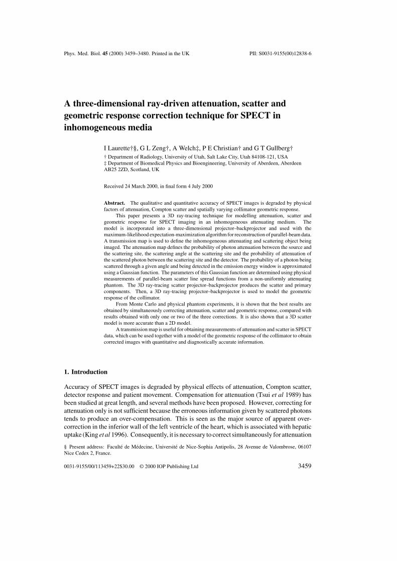
Figure 7. Process of masking images used to compute NSD and contrast.

with a low-energy high-resolution (LEHR) parallel-hole collimator. The characteristics of thecollimator were: thickness = 27 mm, hole radius = 0.7 mm, septal thickness = 0.18 mm.The effects of six orders of scatter were included in the simulation.

The projection data were simulated using an MCAT phantom discretized over 128 slices of128×128 pixels and using 128 1.78 mm wide projection bins. Activity was placed in the liver,the kidneys, the lungs and the myocardium. Seven hundred million counts were simulatedover the 120 views, resulting in a projection set with approximatively 52 × 106 counts perview.

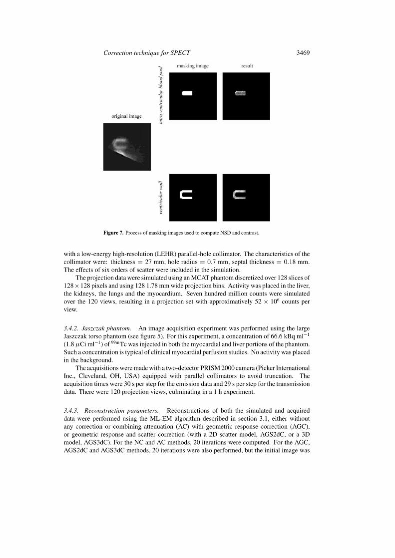
3.4.2. Jaszczak phantom. An image acquisition experiment was performed using the largeJaszczak torso phantom (see figure 5). For this experiment, a concentration of 66.6 kBq ml−1

(1.8µCi ml−1) of 99mTc was injected in both the myocardial and liver portions of the phantom.Such a concentration is typical of clinical myocardial perfusion studies. No activity was placedin the background.

The acquisitions were made with a two-detector PRISM 2000 camera (Picker InternationalInc., Cleveland, OH, USA) equipped with parallel collimators to avoid truncation. Theacquisition times were 30 s per step for the emission data and 29 s per step for the transmissiondata. There were 120 projection views, culminating in a 1 h experiment.

3.4.3. Reconstruction parameters. Reconstructions of both the simulated and acquireddata were performed using the ML-EM algorithm described in section 3.1, either withoutany correction or combining attenuation (AC) with geometric response correction (AGC),or geometric response and scatter correction (with a 2D scatter model, AGS2dC, or a 3Dmodel, AGS3dC). For the NC and AC methods, 20 iterations were computed. For the AGC,AGS2dC and AGS3dC methods, 20 iterations were also performed, but the initial image was


the attenuation corrected reconstructed image. The goal was to shorten the reconstructiontime.

3.5. Data analysis

Several image metrics were used to quantitatively evaluate the scatter correction methods:

• The normalized standard deviation (NSD) in the myocardium containing N voxels wascalculated using:

NSD = 1

f m

√∑Ni (f

mi − f m)2

N − 1(13)

where f m represents the average pixel value in the myocardium. The NSD provides ameasure of uniformity and noise in the myocardium (Beekman et al 1997b).

• The contrast (C) in the myocardium was evaluated using:

C = |f m − f b|f m + f b

(14)

where f b is the average value of the ventricular blood pool.• For a global measure of accuracy of the MCAT (Tsui et al 1994) phantom reconstruction,

the sum of squares of differences (SSD) was calculated for each reconstructed image f r

versus the digital phantom f d :

SSD =N∑i

(f ri − f d

i )2. (15)

• For further quantitative assessment, image profiles through reconstructed images wereplotted.

To compute the NSD and the contrast, a masking image was used to estimate the averagevalue in the myocardium and the ventricular blood pool. For the MCAT study, the maskingimage was the true image itself. For the Jaszczak phantom study, the masking image washeuristically estimated from the reconstructed images (see figure 7).

For all of these computations, the images were first reoriented and then normalized sothat the total number of counts in the reconstructed image was equal to the total number ofcounts in the digitized image for the MCAT experiment and to the total number of counts in theattenuation plus geometric response corrected image for the Jaszczak phantom experiment.

4. Results

From the thresholded reconstructed image, a set of projections was generated using theattenuation, 3D scatter and detector response model described in section 2. Figure 8 shows theestimated line spread functions compared with the acquired data, for four different projectionviews (0, 90, 180 and 270◦). From this figure, it can be seen that a good fit between the dataand the estimated projections is obtained.

Figure 9 presents selected slices through the reconstructed MCAT simulation, comparedwith the original image. The images were first reoriented, to allow the visualization of short-axis and long-axis slices. Profiles through these slices, indicated as white lines in figure 9are presented in figure 10, to compare the different combinations of corrections. In figure 11,profiles of the images reconstructed using the AGS2dC and AGS3dC methods are plotted.


Figure 8. Experimental (dotted curve) and estimated (full curve) line spread functions for the largetorso phantom calculated for four projection views: (a) 0◦, (b) 90◦, (c) 180◦ and (d) 270◦.

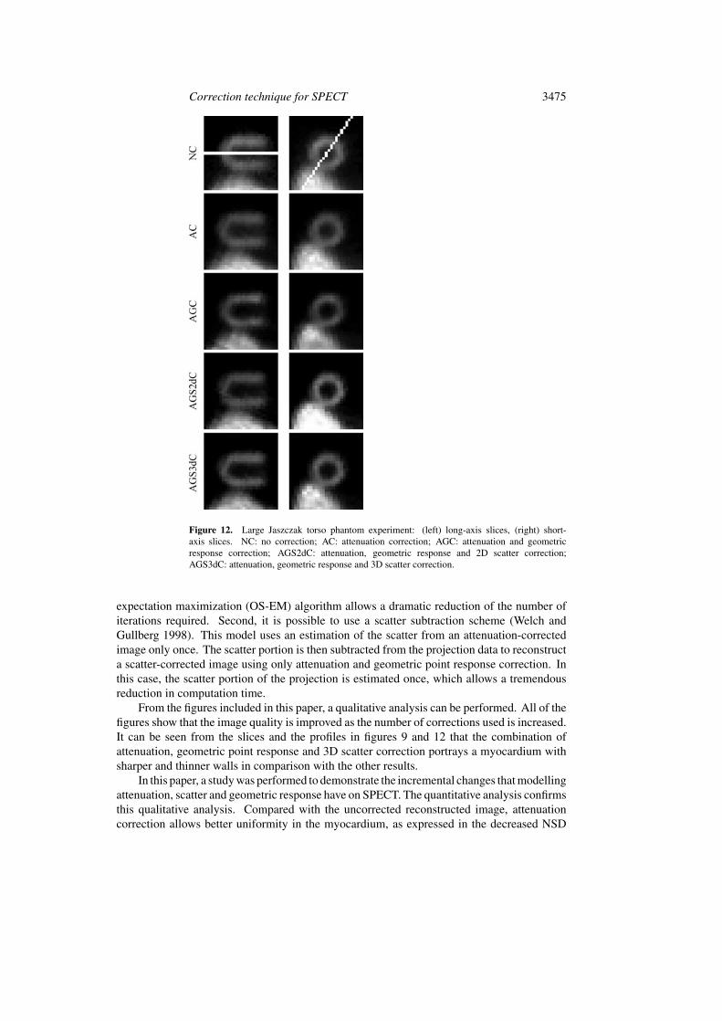
For the Jaszczak phantom, images of short- and long-axis slices are presented in figure 12.The images were also reoriented. Profiles through these slices are presented in figures 13and 14.

From all these figures, an incremental increase of image quality with the number ofcorrections employed can be detected. For the MCAT phantom, the scattered activity aroundthe spine is lowered when scatter correction is used, especially with the 3D scatter model. Thegeometric response correction allows a thinning of the myocardial wall, compared with the NCand AC methods. Including scatter correction with AGS2dC or AGS3dC seems also to increasethe contrast between the left ventricle and the left ventricular chamber. For the Jaszczakphantom, the differences are more difficult to discern because the contrast between the ventricleand the background is modified by the high activity in the liver. However, similar conclusionscan be drawn. Using geometric response correction (AGC) leads to thinner ventricular walls,when compared with NC or AC methods. Including scatter correction (AGS2dC or AGS3dC)makes the reconstructed activity in the ventricle more uniform.


Figure 9. MCAT experiment: (left) long-axis slices, (right) short-axis slices. O: original; NC: nocorrection; AC: attenuation correction; AGC: attenuation and geometric response correction;AGS2dC: attenuation, geometric response and 2D scatter correction; AGS3dC: attenuation,geometric response and 3D scatter correction.

Table 1 shows the results of the quantitative analysis presented in section 3.5. There is noestimation of the SSD for the Jaszczak phantom, since the true distribution is not known. TheAGS3dC method provides the best quantitative results.

5. Discussion and conclusion

In this study we have presented a SPECT reconstruction technique which accounts for non-uniform attenuation, scatter and geometric point response of the detector. The course of aphoton from its emission point to its detection point on the detector can be summarized as:the photon travels through an inhomogeneous medium (the patient body) where it undergoes


Figure 10. MCAT experiment: (top) profiles through long-axis slices (as indicated in figure 9),(bottom) profiles through short-axis slices. NC: no correction; AC: attenuation correction;AGC: attenuation and geometric response correction; AGS2dC: attenuation, geometric responseand 2D scatter correction; AGS3dC: attenuation, geometric response and 3D scatter correction.

Table 1. Quantitative analysis for the MCAT Monte Carlo simulation and the Jaszczak phantomexperiment: computation of contrast (C), normalized standard deviation (NSD) and sum ofsquares of differences (SSD) for the non-corrected image (NC), attenuation corrected image(AC), attenuation plus geometric response corrected image (AGC), and the attenuation, geometricresponse plus scatter corrected image, with the 2D scatter model (AGS2dC) or 3D scatter model(AGS3dC).

MCAT Phantom

C NSD SSD C NSD

NC 0.49 2.53 2.89 × 10−5 0.53 7.61AC 0.51 1.01 2.59 × 10−5 0.51 0.26AGC 0.59 0.57 2.13 × 10−5 0.62 0.21AGS2dC 0.64 0.42 2.04 × 10−5 0.78 0.17AGS3dC 0.69 0.41 1.98 × 10−5 0.83 0.18

several interactions, mostly Compton scatter interactions; after the last interaction, the photontravels to the detector.

The model described in this paper is a sound approximation of the physics of the detectionprocess. First, it takes into account the inhomogeneity of the attenuating media by using theattenuation map reconstructed from the transmission data acquired with the corresponding


Figure 11. MCAT experiment: (top) profiles through long-axis slices (as indicated in figure 9),(bottom) profiles through short-axis slices reconstructed with attenuation, geometric response and2D scatter correction (AGS2dC) or 3D scatter correction (AGS3dC).

emission data. This allows not only an accurate description of the path of a photon from theemission to the detection point, but also a description of its path before and after scattering hasoccurred. Second, the scatter model uses an analytical expression to estimate the distributionof the scattered photons. This model incorporates two approximations: it restricts the processto first-order scattering and the attenuation coefficient M(s) should actually be the electrondensity. However, due to the fit of the scatter probability function to real data, this model alsoprovides a good approximation of the complete distribution of scattered photons as well as otherreal events such as the increase in the attenuation map values after scatter. This scatter modelalso allows a good approximation of the tails of the PSF, but not at the peak. The geometricresponse correction does compensate for this, as can be seen in figure 8. This figure presentsthe experimental and estimated point spread function for a number of positions. The broadshape of the PSF was well reproduced at all of the positions. The point source experimentshows that the complete model presented in this paper fits the experimental data well.

The algorithm was implemented using a ray-driven technique because it is easier tocalculate attenuation factors with the ray-driven technique than it is with the pixel-driventechnique. As the ray travels from the detector through the image voxels it is easy to accumulateline integrals of the attenuation coefficients and to calculate the attenuation factor for each pixel(Gullberg et al 1989). However, this results in long reconstruction times—approximatively 8 hper iteration for a 64×64×30 volume on a Sun Ultra Enterprise 3000 with a 300 MHz processor.Several methods can be used to reduce the computation times. First, the ordered subsets-


Figure 12. Large Jaszczak torso phantom experiment: (left) long-axis slices, (right) short-axis slices. NC: no correction; AC: attenuation correction; AGC: attenuation and geometricresponse correction; AGS2dC: attenuation, geometric response and 2D scatter correction;AGS3dC: attenuation, geometric response and 3D scatter correction.

expectation maximization (OS-EM) algorithm allows a dramatic reduction of the number ofiterations required. Second, it is possible to use a scatter subtraction scheme (Welch andGullberg 1998). This model uses an estimation of the scatter from an attenuation-correctedimage only once. The scatter portion is then subtracted from the projection data to reconstructa scatter-corrected image using only attenuation and geometric point response correction. Inthis case, the scatter portion of the projection is estimated once, which allows a tremendousreduction in computation time.

From the figures included in this paper, a qualitative analysis can be performed. All of thefigures show that the image quality is improved as the number of corrections used is increased.It can be seen from the slices and the profiles in figures 9 and 12 that the combination ofattenuation, geometric point response and 3D scatter correction portrays a myocardium withsharper and thinner walls in comparison with the other results.

In this paper, a study was performed to demonstrate the incremental changes that modellingattenuation, scatter and geometric response have on SPECT. The quantitative analysis confirmsthis qualitative analysis. Compared with the uncorrected reconstructed image, attenuationcorrection allows better uniformity in the myocardium, as expressed in the decreased NSD


Figure 13. Large Jaszczak torso phantom experiment: (top) profiles through long-axisslices (as indicated in figure 12), (bottom) profiles through short-axis slices. NC: nocorrection; AC: attenuation correction; AGC: attenuation and geometric response correction;AGS2dC: attenuation, geometric response and 2D scatter correction; AGS3dC: attenuation,geometric response and 3D scatter correction.

ratio (2.53 versus 1.01 for the MCAT, and 7.61 versus 0.26 for the Jaszczak phantom). Thisimproved uniformity is due to better equalization of the levels of the septal and inferior walls.Combining the geometric response and the scatter model preserves this property. As expected,attenuation does not ameliorate the contrast. This can be explained simply by the fact that boththe background and the myocardium values are corrected in the same way when attenuation istaken into account. Compared with attenuation correction, geometric point response correctiondoes not actually improve the uniformity in the myocardium. However, the slightly betterNSD value can be explained by the fact that geometric point response correction requires moreiterations in order to be efficiently employed in the reconstruction process (Wilson and Tsui1994). As can be seen in the slices and the profiles, the major influence of correcting for thegeometric point response is to thin the walls of the myocardium. Finally, scatter correction hasa major impact on contrast quality. This factor is dramatically improved in both the MCATand the Jaszczak phantom experiments.

The developed model fully incorporates the three-dimensional nature of the problem. Ithas already been shown that a 3D model outperforms a 2D model (Beekman et al 1996).From the results presented here, it can be seen in figures 11 and 14, and table 1 that the 3Dmodel yields the best quantification of the figures of merit we were interested in. This iscaused by the high concentration value in the liver which affects the true value located in themyocardium.


Figure 14. Large Jaszczak torso phantom experiment: (top) profiles through long-axis slices (asindicated in figure 12), (bottom) profiles through short-axis slices reconstructed with attenuation,geometric response and 2D scatter correction (AGS2dC) or 3D scatter correction (AGS3dC).

This paper describes a comprehensive method that accounts for the major degrading effectsin SPECT: attenuation, scatter and detector geometric response. We have demonstrated theincremental changes that attenuation correction, scatter correction and geometric responsecorrection have on SPECT. We have also compared the influence of a 3D scatter model witha 2D model, and found the 3D model to be superior. However, a more thorough evaluationis necessary to effectively measure the importance of this factor. Also, we will work todemonstrate the importance of modelling non-uniform attenuation between the source andscatter point, as opposed to methods that assume a uniform attenuator (Frey and Tsui 1996).

Acknowledgments

This work was supported in part by the National Institutes of Health under grant RO1 HL 39792,and Picker International. We want to thank Sean Webb for carefully proof reading themanuscript.

References

Axelsson B, Msaki P and Israelsson A 1984 Subtraction of Compton-scatter photons in single-photon emissioncomputerized tomography J. Nucl. Med. 25 490–4

Bai C, Zeng G L and Gullberg G T 2000 A slice-by-slice blurring model and kernel evaluation using Klein–Nishinaformula for 3D scatter compensation in parallel and converging beam SPECT Phys. Med. Biol. 45 1275–307


Bai C, Zeng G L, Gullberg G T, DiFilippo F and Miller S 1998 Slab-by-slab blurring model for geometric pointresponse correction and attenuation correction using iterative reconstruction algorithm IEEE Trans. Nucl. Sci.45 2168–73

Beekman F J, den Harder J M, Viergever M A and van Rijk P P 1997a SPECT scatter modelling in non-uniformattenuating objects Phys. Med. Biol. 42 1133–42

Beekman F J, Eijkman E, Viergever M A, Borm G and Slijpen E 1993 Object shape dependent PSF model for SPECTimaging IEEE Trans. Nucl. Sci. 40 31–9

Beekman F J, Frey E C, Kamphuis C, Tsui B M W and Viergever M A 1994 A new phantom for fast determinationof scatter response of a gamma camera IEEE Trans. Nucl. Sci. 41 1481–8

Beekman F J, Kamphuis C and Frey E C 1997b Scatter compensation methods in 3D iterative SPECT reconstruction:A simulation study Phys. Med. Biol. 42 1619–32

Beekman F J, Kamphuis C and Viergever M A 1996 Improved SPECT quantitation using fully three-dimensionaliterative spatially variant scatter response compensation IEEE Trans. Med. Imaging 15 491–9

Beekman F J and Viergever M A 1995 Fast SPECT simulation including object shape dependent scatter IEEE Trans.Med. Imaging 14 271–82

Bowsher J E and Floyd C E 1991 Treatment of Compton scatter in maximum-likelihood, expectation-maximizationreconstruction of SPECT images J. Nucl. Med. 32 1285–91

Cao Z-J, Frey E C and Tsui B M W 1994 A scatter model for parallel and converging beam SPECT based on theKlein–Nishina formula IEEE Trans. Nucl. Sci. 41 1594–600

DeVito R P, Hamill J J, Treffert J D and Stoub T W 1989 Energy-weighted acquisition of scintigraphic images usinga finite spatial filter J. Nucl. Med. 30 2029–35

Elmbt L V and Walrand S 1993 Simultaneous correction of attenuation and distance-dependant collimator blurringPhys. Med. Biol. 38 1207–17

Floyd C E, Jaszczak R J and Coleman R E 1985a Inverse Monte Carlo: a unified reconstruction algorithm IEEE Trans.Nucl. Sci. 32 779–85

——1986 Inverse Monte Carlo as a unified reconstruction algorithm for ECT J. Nucl. Med. 27 1577–85——1987 Maximum likelihood reconstruction for SPECT with Monte Carlo modelling: asymptotic behaviour IEEE

Trans. Nucl. Sci. 34 285–7——1989 Inverse Monte Carlo: a unified reconstruction algorithm IEEE Trans. Nucl. Sci. 32 779–85Floyd C E, Jaszczak R J, Greer K L and Coleman R E 1985b Deconvolution of Compton scatter in SPECT J. Nucl.

Med. 26 403–8Floyd C E, Jaszczak R J, Harris C C and Coleman R E 1984 Energy and spatial distribution of multiple order Compton

scatter in SPECT: a Monte Carlo investigation Phys. Med. Biol. 29 1217–30Formiconi A R, Pupi A and Passeri A 1989 Compensation of spatial system resolution in SPECT with conjugate

gradient techniques Phys. Med. Biol. 34 69–84Frey E C, Ju Z W and Tsui B M W 1993 A fast projector–backprojector pair modelling the asymmetric, spatially

varying scatter response function for scatter compensation in SPECT imaging IEEE Trans. Nucl. Sci. 40 1192–7Frey E C and Tsui B M W 1990 Parametrization of the scatter response function in SPECT imaging using Monte

Carlo simulation IEEE Trans. Nucl. Sci. 37 1308–15——1993 A practical method for incorporating scatter in a projector–backprojector for accurate scatter compensation

in SPECT IEEE Trans. Nucl. Sci. 40 1107–16——1994 Modelling the scatter response function in inhomogeneous scattering media for SPECT IEEE Trans. Nucl.

Sci. 41 1585–93——1996 A new method for modelling the spatially-variant, object dependent scatter response function in SPECT

Record 1996 IEEE Nuclear Science Symp. Medical Imaging Conf. (Piscataway, NJ: IEEE) pp 1082–6Frey E C, Tsui B M W and Ljungberg M 1992 A comparison of scatter compensation methods in SPECT: substraction-

based techniques versus iterative reconstruction with accurate modelling of the scatter response Record 1992IEEE Nuclear Science Symp. Medical Imaging Conf. (Piscataway, NJ: IEEE) pp 1305–7

Gagnon D, Todd-Pokropek A, Milanesi L and Fazio F 1989 Introduction to holospectral imaging in nuclear medicinefor scatter substraction IEEE Trans. Med. Imag. 8 245–50

Gilland D R, Jaszczak R J, Wang H, Turkington T G, Greer K L and Coleman R E 1994 A 3D model of non-uniformattenuation and detector response for efficient iterative reconstruction in SPECT Phys. Med. Biol. 39 547–61

Gilland D R, Tsui B M W, McCartney W H and Perry J R 1988 Determination of the optimum filter function forSPECT imaging J. Nucl. Med. 29 643–50

Glick S J, Penney B C, King M A and Byrne C L 1994 Noniterative compensation for the distance-dependant detectorresponse and photon attenuation in SPECT imaging IEEE Trans. Med. Imag. 13 363–74

Gullberg G T, Hsieh Y-L and Zeng G L 1996 An SVD reconstruction algorithm using a natural pixel representationof the attenuated Radon transform IEEE Trans. Nucl. Sci. 43 295–303


Gullberg G T, Huesman R H, Malko J A, Pelc N J and Budinger T F 1985 An attenuated projector–backprojector foriterative SPECT reconstruction Phys. Med. Biol. 8 799–816

Gullberg G T, Huesman R H, Ross S G, DiBella E V R, Zeng G L, Reutter B W, Christian P E and Foresti S A1998 Dynamic cardiac single photon emission computed tomography Nuclear Cardiology: State of the Art andFuture Direction (St Louis, MO: Mosby) pp 137–87

Gullberg G T, Zeng G L, Tsui B M W and Hagius J T 1989 An iterative reconstruction algorithm for single photonemission computed tomography with cone beam geometry Int. J. Imaging Syst. Tech. 1 169–86

Halama J R, Henkin R E and Friend L E 1988 Gamma camera radionuclide images: improved contrast with energy-weighted acquisition Radiology 169 533–8

Hamill J J and DeVito R P 1989 Scatter reduction with energy weighted acquisition IEEE Trans. Nucl. Sci. 36 1334–9Hsieh Y-L, Zeng G L and Gullberg G T 1998 Projection space image reconstruction using strip functions to calculate

pixels more ‘natural’ for modelling the geometric response of the SPECT collimator IEEE Trans. Med. Imaging17 24–44

Hutton B F 1997 Cardiac single-photon emission tomography: is attenuation correction enough? Eur. J. Nucl. Med.24 713–15

Hutton B F, Osiecki A and Meikle S R 1996 Transmission-based scatter correction of 180 degree myocardial single-photon emission tomographic studies Eur. J. Nucl. Med. 23 1300–8

Jaszczak R J, Floyd C E and Coleman R E 1985 Scatter compensation techniques for SPECT IEEE Trans. Nucl. Sci.32 786–93

Jaszczak R J, Greer K L, Floyd C E, Harris C C and Coleman R E 1984 Improved SPECT quantification usingcompensation for scattered photons J. Nucl. Med. 25 893–9

Ju Z W, Frey E C and Tsui B M W 1995 Distributed 3-D iterative reconstruction for quantitative SPECT IEEE Trans.Nucl. Sci. 42 1301–9

Kadrmas D J, DiBella E V R, Huesman R H and Gullberg G T 1999 Analytical propagation of errors in dynamicSPECT: estimators, degrading factors, bias and noise Phys. Med. Biol. 44 1997–2014

Kadrmas D J, Frey E C, Karimi S S and Tsui B M W 1998 Fast implementations of reconstruction-based scattercompensation in fully 3D SPECT image reconstruction Phys. Med. Biol. 43 857–74

Kadrmas D J, Frey E C and Tsui B M W 1996 An SVD investigation of modelling scatter in multiple energy windowsfor improved SPECT images IEEE Trans. Nucl. Sci. 43 2275–84

——1997 Analysis of the reconstructibility and noise properties of scattered photons in 99mTc SPECT Phys. Med.Biol. 42 2493–516

King M A, Doherty P W, Schwinger R B, Jacobs D A, Kidder R E and Miller T R 1983 Fast count-dependant digitalfiltering of nuclear medicine images: concise communication J. Nucl. Med. 24 1039–45

King M A, Hadenomos G J and Glick S J 1992 A dual-photopeak window method for scatter correction J. Nucl. Med.33 605–12

King M A, Schwinger R B, Doherty P W and Penny B C 1984 Two-dimensional filtering of SPECT images using theMetz and Wiener filters J. Nucl. Med. 25 1234–40

King M A, Xia W, de Vries D J, Pan T-S, Villegas B J, Dahlberg S, Tsui B M W, Ljunberg M H and Morgan H T 1996 AMonte Carlo investigation of artifacts caused by liver uptake in SPECT perfusion imaging with Tc-99m-labelledagents J. Nucl. Cardiol. 3 18–29

Koral K F, Swailem F M, Buchbinder S, Clinthorne N H, Rogers W L and Tsui B M W 1990 SPECT dual-energy-window Compton correction: scatter multiplier required for quantification J. Nucl. Med. 31 90–8

Koral K F, Wang X, Rogers W L, Clinthorne N H and Wang X 1988 SPECT Compton-scattering correction by analysisof energy spectra J. Nucl. Med. 29 195–202

Lewitt R M, Edholm P R and Xia W 1989 Fourier method for correction of depth-dependant collimator blurring Proc.SPIE 1092 232–43

Lowry C A and Cooper M J 1987 The problem of Compton scattering in emission tomography: a measurement of itsspatial distribution Phys. Med. Biol. 32 1187–91

Meikle S R, Hutton B F and Bailey D L 1994 A transmission-dependent method for scatter correction in SPECTJ. Nucl. Med. 35 360–7

Metz C E, Atkins F B and Beck R N 1980 The geometric transfer function component for scintillation cameracollimators with straight parallel holes Phys. Med. Biol. 25 1059–70

Msaki P, Axelsson B, Dahl C M and Larsson S A 1987 Generalized scatter correction method in SPECT using pointscatter distribution functions J. Nucl. Med. 28 1861–9

Msaki P, Axelsson B and Larsson S A 1989 Some physical factors influencing the accuracy of convolution scattercorrection in SPECT Phys. Med. Biol. 34 283–98

Ogawa K, Harata Y, Ichihara T, Kubo A and Hashimoto S 1991 A practical method for position-dependent Compton-scatter correction in single photon emission CT IEEE Trans. Med. Imag. 10 408–12


Ogawa K, Paek S, Nakajima M, Yuta S, Kubo A and Hashimoto S 1988 Correction of collimator aperture using ashift-invariant deconvolution and filter in gamma camera emission CT Proc. SPIE 914 699–706

Riauka T A and Gortel Z W 1994 Photon propagation and detection in single-photon emission computed tomography:an analytical approach Med. Phys. 21 1311–22

Riauka T A, Hooper H R and Gortel Z W 1996 Experimental and numerical investigation of the 3D SPECT photondetection kernel for non-uniform attenuating media Phys. Med. Biol. 41 1167–89

Tsui B M W and Gullberg G T 1990 The geometric transfer function for cone and fan beam collimators Phys. Med.Biol. 35 81–93

Tsui B M W, Gullberg G T, Edgerton E R, Ballard J G, Perry J R, McCartney W H and Berg J 1989 Correction ofnonuniform attenuation in cardiac SPECT imaging J. Nucl. Med. 28 497–507

Tsui B M W, Hu H D, Gilland D R and Gullberg G T 1988 Implementation of simultaneous attenuation and detectorresponse correction in SPECT IEEE Trans. Nucl. Sci. 35 778–83

Tsui B M W, Zhao X D, Gregoriou G K, Lalush D S, Frey E C, Johnston R E and McCartney W H 1994 Quantitativecardiac SPECT reconstruction with reduced image degradation due to patient anatomy IEEE Trans. Nucl. Sci.41 2838–44

Vannoy S 1994 The Photon History Generator (The Imaging Research Lab, University of Washington Medical Center)Veklerov E, Llacer J and Hoffman E 1988 MLE reconstruction of a brain phantom using a Monte Carlo transition

matrix and a statistical stopping rule Trans. Nucl. Sci. 35 603–7Walrand S H M, Elmbt L V and Pauwels S 1994 Quantification in SPECT using an effective model of the scattering

Phys. Med. Biol. 39 719–34Welch A and Gullberg G T 1998 Implementation of a model-based non-uniform scatter correction scheme for SPECT

IEEE Trans. Med. Imaging 16 717–26Welch A, Gullberg G T, Christian P E, Datz F L and Morgan H T 1995 A transmission-map-based scatter correction

technique for SPECT in inhomogeneous media Med. Phys. 22 1627–35Wells R G, Celler A and Harrop R 1997 Experimental validation of an analytical method of calculating SPECT

projection data IEEE Trans. Nucl. Sci. 44 1283–90——1998 Analytical calculation of photon distributions in SPECT projections IEEE Trans. Nucl. Sci. 45 3202–14Wilson D W and Tsui B M W 1994 Spatial resolution properties of FB and ML-EM reconstruction methods Proc.

1993 IEEE Nuclear Science Symp. and Medical Imaging Conf. (Piscataway, NJ: IEEE) pp 1189–93Xia W, Lewitt R M and Edholm P R 1995 Fourier correction for spatially variant collimator blurring in SPECT IEEE

Trans. Med. Imag. 14 100–15Zeng G L, Bai C and Gullberg G T 1999 A projector/backprojector with slice-to-slice blurring for efficient 3D scatter

modelling IEEE Trans. Med. Imag. 18 722–32Zeng G L, Gullberg G T, Bai C, Christian P E, Trisjono F, DiBella E V R, Tanner J W and Morgan H T 1998 Iterative

reconstruction of fluorine-18 SPECT using geometric point response correction J. Nucl. Med. 39 124–30Zeng G L, Gullberg G T, Tsui B M W and Terry J A 1991 Three-dimensional iterative reconstruction algorithms with

attenuation and geometric point response correction IEEE Trans. Nucl. Sci. 38 693–702

A three-dimensional ray-driven attenuation, scatter and...

Documents

Transcript of A three-dimensional ray-driven attenuation, scatter and...