A Thesis Submitted for the Degree of PhD at the University...

University of Warwick institutional repository: http://go.warwick.ac.uk/wrap

A Thesis Submitted for the Degree of PhD at the University of Warwick

http://go.warwick.ac.uk/wrap/72837

This thesis is made available online and is protected by original copyright.

Please scroll down to view the document itself.

Please refer to the repository record for this item for information to help you tocite it. Our policy information is available from the repository home page.

http://go.warwick.ac.uk/wrap

http://go.warwick.ac.uk/wrap/72814

The Use of Ligand Field Molecular Mechanics and Related Tools in the

Design of Novel Spin Crossover Complexes

By

Benjamin John Houghton

A thesis submitted in partial fulfilment of the requirements for the

degree of Doctor of Philosophy in Chemistry

Department of Chemistry,

University of Warwick,

CV4 7AL

April 2015

i

Contents

Tables and Illustrations .......................................................................................................... 1

Acknowledgments ................................................................................................................ 14

Declaration ........................................................................................................................... 15

Abstract ................................................................................................................................ 17

Abbreviations ....................................................................................................................... 19

Chapter 1: An Introduction to Spin Crossover ..................................................................... 20

Fe(II) Monomeric Species ................................................................................................ 22

Metals other than iron(II) .................................................................................................. 34

Chapter 2: Theoretical Approaches to Spin Crossover. ....................................................... 39

Density Functional Theory – A theoretical background ................................................... 39

Performance of Functionals for Spin Crossover Research ............................................... 43

Hybrid Methods ................................................................................................................ 46

Basis Set Effects ............................................................................................................... 48

High Level Approaches .................................................................................................... 49

Modelling Spin Transitions of Bulk Lattices .................................................................... 50

What is the alternative?..................................................................................................... 50

Chapter 3: An Introduction to Ligand Field Molecular Mechanics ..................................... 51

Introduction ....................................................................................................................... 51

Molecular Mechanics ........................................................................................................ 52

LFMM – The methodology .............................................................................................. 53

Cu(II) Amines ................................................................................................................... 54

ii

The Angular Overlap Model ............................................................................................. 55

Implementation in the Molecular Operating Environment with the test case [MCl4]2-

.... 58

Ruthenium Arenes ............................................................................................................ 60

Automated Parameter Optimisation.................................................................................. 61

Spin Crossover .................................................................................................................. 65

Alternate Approaches in the Literature ............................................................................. 66

Concluding Remarks......................................................................................................... 67

Chapter 4: Traversing the Density Functional Minefield .................................................... 68

An Introduction ................................................................................................................. 68

Does One Functional Suit All Problems? ......................................................................... 68

How can calculations of spin-state energetics be improved? ........................................... 71

R,R’Pytacn Complexes an Application of Density Functional Theory to Spin Crossover

Problems ........................................................................................................................... 82

Conclusions ....................................................................................................................... 85

Chapter 5; The Use of Force Field Based Methods for the Study of Transition Metal

Complexes ............................................................................................................................ 86

Introduction ....................................................................................................................... 86

Computational Details ...................................................................................................... 91

Force Field Sensitivity Testing ......................................................................................... 92

Molecular Dynamics in LFMM ........................................................................................ 94

The construction of a mixed amine/imine force field for Fe(II) ....................................... 99

The use of Hammett sigma values in LFMM ................................................................. 110

Improving the Handley force field .................................................................................. 113

iii

Addressing the stiff iron-nitrogen-carbon angle term..................................................... 122

Increasing the Transferability ......................................................................................... 125

Chapter 6 – The Design of Novel Transition Metal Complexes through Ligand Generation

............................................................................................................................................ 130

The parameterisation of a robust cobalt(II) force field ................................................... 132

Computational Details .................................................................................................... 132

Results and Discussion ................................................................................................... 139

True high throughput screening ...................................................................................... 150

The Candidates ............................................................................................................... 164

Conclusions ..................................................................................................................... 177

Chapter 7 – Conclusion ...................................................................................................... 179

References: ......................................................................................................................... 183

Appendix 1 – ADFs Functionals (called by the METAGGA and HARTREEFOCK

Keywords) and their References as extracted from an ADF output. ................................. 194

Appendix 2 - The Use of DommiMOE as a Ligand Generation Tool ............................... 202

1

Tables and Illustrations

Figure 1.1; The ligand shown by Young et al to display promise in barbiturate sensing.8,9

21

Figure 1.2; The 1,10-phenanthrolene ligand upon which the first iron(II) SCO complex was

based.11

................................................................................................................................. 21

Figure 1.3; The possible three d-electron configurations of an octahedral d6 complex.

Clockwise these are high spin (5T2), intermediate spin (

3T1) and low spin (

1A1). In the case

of octahedral iron(II) the intermediate spin state is inaccessible. ........................................ 23

Figure 1.4; The Tanabe-Sugano diagram for d6 species.

13 (Note the

3T1 and

5T2 states are

referred to by the older 3F1 and

5F2 levels respectively, also Fe(III) is an old reference to

Fe(II)). Figure reproduced with permission of The Physical Society of Japan. .................. 24

Figure 1.5; Three typical spin transition curves expressed as the fraction of the sample

which is HS as a function of temperature. Top left: a gradual spin transition.15

Top right: an

abrupt spin transition of a bulk sample.15

Bottom centre: an example of hysteresis were the

transition occurs at a different temperature upon heating when compared to cooling.15

..... 26

Figure 1.6; [Fe(btz)2(NCS)2] on the left and the btz ligand on the right.20

.......................... 27

Figure 1.7; a representation of trans-[Fe(4-p-methylphenyl-3,5-bis(pyridin-2-yl)-1,2,4-

triazole)2(NCS)2] on the left and the 4-p-methylphenyl-3,5-bis(pyridin-2-yl)-1,2,4-triazole

ligand on the right.23

............................................................................................................. 28

Figure 1.8; [Fe(dpp)2(NCS)2] on the left and the dpp ligand on the right.24

........................ 29

Figure 1.9; The ligand utilised by Müller in the synthesis of the [FeL(Him)2] SCO

complex.27

............................................................................................................................ 30

Figure 1.11; The ligand 2,2’-bi-2-imidazoline for which SCO in the solid state is dictated

by choice of counter ion.32

................................................................................................... 31

Figure 1.12; A pictorial representation of the 2,2′-bi-1,4,5,6-tetrahydropyrimidine ligand.6

.............................................................................................................................................. 32

Figure 1.13; The iron(II) complexes of the 3-bpp ligand on the left and 1-bpp ligand on the

2

right were studied by the Halcrow group in a range of solvents.34

...................................... 32

Figure 1.14; The tris(1-(2-azolyl)-2-azabuten-4-yl)amine used in the first Mn(III) SCO

complex. ............................................................................................................................... 34

Figure 1.15; The general structure of iron(III) dithiocarbamates where R denotes any alkyl

group.46,47

............................................................................................................................. 36

Figure 1.16; The non-innocent o-aminophenol derived ligand which was shown to

facilitate SCO by Chaudhuri et al.48

..................................................................................... 36

Figure 1.17; The porphyrin ring based ligand used to facilitate room temperature spin state

bistability.29,56

....................................................................................................................... 38

Figure 2.1; Left is the model complex used in the Neese group’s study whilst on the right is

the complex from which the experimental results were obtained.61

.................................... 45

Figure 2.2; A comparison of the structure of high spin [Fe(N2H4)(NHS4)]0 given by X-ray

diffraction on the left and that used by Neese in his calculations on the right.61,78

............. 45

Figure 2.3; The complexes used in Reiher’s reparameterisation of B3LYP. For L = NH3

and N2H4 a cis-geometry is adopted while for L = CO, NO+, PH3 and PMe3 a trans-

geometry is adopted. ............................................................................................................ 47

Figure 3.1; Left the octahedral geometry with two unique A-M-A angles and right a

trigonal bipyramidal geometry with three unique angles.97

................................................. 53

Figure 3.2; The ligand and LFMM regions and the angle and torsional terms spanning it.96

.............................................................................................................................................. 53

Figure 3.3; The effect of tetragonal elongation on the eg orbitals of an octahedral species.93

.............................................................................................................................................. 54

Figure 3.4; The definitions of the angles employed in determining the magnitude of F2.97

56

Figure 3.5: The effect of a ligand’s orientation with respect to the z axis in destabilising the

dz2 orbital as a proportion of eσ97

. The y-axis represents Fσ2dz2 as shown in Equation 3.3.

.............................................................................................................................................. 57

3

Figure 3.6; The effect of distortion on the metal d-orbitals of tetrahedral species, on the left

[NiCl4]2-

, a d8 species displaying a D2d distortion and on the right the d-orbitals of

compressed [CuCl4]2-

.96

........................................................................................................ 59

Figure 3.8; A representation of the ruthenium arene complexes studied by Brodbeck and

Deeth.103

............................................................................................................................... 60

Figure 3.09; A depiction of ΔEHL, the difference in energy between the high and low spin

forms of a metal complex.1 .................................................................................................. 62

Figure 3.10; On the left a pictorial representation of the improvement of parameters in the

objectives over time, illustrated as three idealised generations. On the right the distinction

between the lowest ranked Pareto fronts.1,110

....................................................................... 64

Figure 3.11; A depiction of the training set used in the initial iron(II) SCO force field.94

.. 65

Figure 4.1; The ligands associated with the five SCO complexes studied. ......................... 69

Table 4.1; The calculated spin state splittings as calculated for five SCO complexes

through POST-SCF calculations on OPBE optimised geometries. References for all 75

functionals are included in Appendix 1. .............................................................................. 70

Figure 4.2; A definition of spin state splitting (ΔEHL) and the zero point energy correction.

.............................................................................................................................................. 71

Figure 4.3; The five iron(II) hexamine complexes studied for which the ground states span

the SCO divide. The five compounds are DETTOL (6), PURYIK (7), PAZXAP (8), Fe399

(9) and FEBPYC (10). ......................................................................................................... 73

Table 4.2; A comparison of the effects of inclusion of dispersion and solvation on the

calculated iron nitrogen bond lengths (Å) of four iron(II) amines which span the SCO

divide. ................................................................................................................................... 74

Table 4.3; The values of ΔEHL (kcal mol-1

) as calculated using the BP86 functional, Def2-

SVP basis set and Def2-SVP/J auxiliary basis set in conjunction with various corrections

in. .......................................................................................................................................... 75

4

Figure 4.4; The spin state splittings (ΔEHL) of the four complexes studied using the BP86

functional, Def2-SVP basis set and Def2-SVP/J auxiliary basis set in conjunction with the

COSMO solvation model scaled by 16 kcal mol-1

to ensure DETTOL is SCO. ................. 75

Table 4.4; The basis set dependence of ΔEHL when using slater type basis sets ADF

(Version 2012.01120

and OPBE with COSMO(water). ........................................................ 76

Figure 4.5. The effect of the damping function on dispersion contributions to calculated

interaction potentials.136

....................................................................................................... 77

Table 4.5; The effect of varying s6 on calculated binding energetics in kcal mol-1

for

OPBE. .................................................................................................................................. 79

Figure 4.6: A plot of MAD as a function of the s6 parameter. ............................................. 80

Figure 5.1; The five iron(II) hexamine complexes used as training data in the

parameterisation of iron(II) amine bonds for LFMM along with their references. ............. 87

Figure 5.2; Final Pareto front of the second 50 generation optimisation run with each point

marks a Pareto optimal parameter set from which the parameters in Table 5.1 were taken.

.............................................................................................................................................. 90

Table 5.1; The proposed parameter set derived from the optimisation run of Figure 5.2 for

which the energetic RMSD is 0.90 kcal mol-1

and the structural RMSD is 0.059 Å. The

values are reported in their full length as obtained from the parameter optimisation. Their

sensitivity to variation will be explored in the next section. ................................................ 90

Table 5.2; The effects of a ten percent variation in each parameter on the energetic and

geometric penalty functions. It is important to note that whilst the numbers are reported to

an appropriate number of significant figures the underlying variations were based on the

raw parameter values from the parameter optimisation run................................................. 92

Table 5.3; The force field parameters used by Robert J. Deeth for the LFMD run are those

found in the paper of Deeth et al 201094

and are given in this table. ................................... 94

Figure 5.3; The recorded energies relative to t=0 of the last 10 ps of the LS structure at 360

5

K. The “correction” is a transposition by 6.23 kcal mol-1

(the average of the last 10 ps DFT

energetics, included purely for illustration). ........................................................................ 95

Figure 5.4; The recorded energies relative to t=0 of the last 10 ps of the HS structure at 360

K. The “correction” is a transposition by 8.17 kcal mol-1

(the average of the last 10 seconds

DFT energetics, included purely for illustration). ................................................................ 96

Figure 5.5; A plot of DFT energies (relative to the energy at t=0) and the LFMM energy

(relative to the energy at t=0) at the same geometry as obtained from the last 10ps of the

high spin LFMD run at 360K. .............................................................................................. 96



low spin LFMD run at 360K. ............................................................................................... 97

Table 5.4; Spin state splittings for DETTOL averaged over the last 10 ps of a 200 ps run.98

Table 5.5: The effect of basis set on the geometry of the low and high spin states of

APEFEH with the distances given in Å. The RI approximation was utilised and so the

corresponding auxiliary basis sets were also used (def2-SVP/J and def2-TZVP/J as

appropriate). ....................................................................................................................... 100

Table 5.6: The spin state splitting, ΔEHL, of the training complexes. Note that the

calculations on MELLOF07, QOQHEK and WIGPOR were carried out by Professor

Robert J. Deeth. .................................................................................................................. 100

Figure 5.7; The eight pyridine/amine ligands used to form octahedral iron(II) complexes.

............................................................................................................................................ 101

Figure 5.8; A plot of the final Pareto front of a fifty generation parameter optimisation run.

The amine parameters were kept fixed while pyridine parameters varied......................... 102

Figure 5.9: Two plots displaying Pareto Front 1 of the 50th Generation of three parameter

optimisation runs in which the amine electron pairing parameter was allowed to vary. The

first plot is across all values of the penalty functions while the second is across the region

6

of interest. The first optimises pyridine parameters taking the amine parameters as a

starting point (X), the second uses the same starting point excluding CEYRAA (+) and the

third takes a parameter set from the second run and further optimises it (○). ................... 104

Table 5.7; Parameter set 21 from the second optimisation run without CEYRAA. .......... 105

Table 5.8; Parameter set 34 from the second optimisation run without CEYRAA. .......... 105

Table 5.9; The performance of parameter set 21 (2.00 kcal mol-1

energetic RMSD and

0.0624 Å structural RMSD) of Run 2 without CEYRAA in the training set..................... 106


energetic RMSD and

0.0707 Å structural RMSD) of Run 2 without CEYRAA in the training set..................... 106

Table 5.11; Parameter set 15 from the first optimisation run without CEYRAA. This set is

recommended for those interested only in geometric accuracy. ........................................ 107

Figure 5.10; A plot of LFMM derived spin state splittings against DFT for parameter set

21. ....................................................................................................................................... 108


34. ....................................................................................................................................... 108

Table 5.12; The four complexes used as a test of the transferability of the mixed force

field. Optimised in ORCA with OPBE COSMO(water) RI def2-TZVP def2-TZVP/J .... 109

Table 5.13; The spin-state splittings of iron(II) tris(2,2'-bipyridine) substituted on all six

para positions. .................................................................................................................... 111

Figure 5.12 – A plot of the OPBE and BP86 spin-state splittings relative to the value for

the para-amine species as a function of Hammett sigma values. ....................................... 112

Table 5.14; The calculated Mulliken charges for the four crystallographically characterised

complexes in the original Handley and Deeth paper. The coordinated charges are obtained

from SPE calculations (OPBE, TZP) on previously optimised structures (BP86, RI

approximation, Def2-SVP, Def2-SVP/J auxiliary basis set and COSMO epsilon 80

refractive index 1.33 (water 80.4 and 1.33 respectively)). The uncoordinated charges were

7

calculated solvent free based on single point calculations (OPBE, TZP) on the free ligands

based on their LS derived structures. ................................................................................. 114

Figure 5.23; The effect of the use of bond charge increments on MMFF94 charges. ....... 115

Figure 5.24; A plot of energetic RMSD against geometric RMSD for Pareto front 1 of the

50th

generation of the second parameter optimisation of a charged iron(II) amine force

field. ................................................................................................................................... 116

Figure 5.25; Top left are the charges on the nitrogen and hydrogens of ammonia and top

right the charges of protonated ammonia, NH4+. Bottom left is the charges in the transition

metal MMFF94 (without a Fe-N BCI) and right the charges under the PSML routine..... 117

Table 5.15; The Natural Charges160,161

on iron in a range of iron(II) amine complexes as

obtained from Gaussian 03.163

............................................................................................ 117

Figure 5.26; A plot of Pareto front 1 from the 100th

generation of the second parameter

optimisation run. ................................................................................................................ 119

Table 5.16; Parameter set 19 from Figure 5.26, with an energetic RMSD of 0.73 kcal mol-1

and a geometric RMSD of 0.067 Å. ................................................................................... 120

Table 5.17; The metal-ligand and heavy atom RMSDs for the iron(II) amine training set

when using parameter set 19. Distances in Å. ................................................................... 120

Figure 5.27; A superposition of the two complexes with the highest heavy atom RMSD for

Parameter Set 19. HS PAZXAP is shown on the left with a heavy atom RMSD of 0.13 Å.

Right is HS PURYIK with a heavy atom RMSD of 0.18 Å. ............................................. 121

Table 5.18; The parameter set for which an energetic RMSD of 0.24 kcal mol-1

and a

geometric RMSD of 0.065 Å is obtained using the Fe+2

-N-C force constant of

200 kcal mol-1

deg-2

. ........................................................................................................... 123

Table 5.19; The energetic and geometric data obtained after altering the iron(II)-N-C force

constant from 200 to 30 kcal mol-1

deg-2

. .......................................................................... 123

Figure 5.28; The final Pareto front of the fifty generation optimisation run with a reduced

8

bond angle force constant................................................................................................... 124

Figure 5.29; The HS crystal structure of tris(1,2-diaminobenzene) iron(II)165

.................. 125

Figure 5.30; The direction of the nitrogen p-orbital containing the lone pair in

uncoordinated amino benzene. ........................................................................................... 126

Figure 5.31; A plot of 1+cos(2x) to illustrate the second term scaled by V2/2. ................ 127

Figure 5.32; Plots of the effect of varying the torsional constants V1/2, V2/2 and V3/2 on

the heavy atom RMSD of LFMM structures from the DFT reference structures. ............. 128

Figure 5.33; The overlap of the crystal structure165

and the high spin LFMM structure

using the new Fe-N-Car-Car torsional force constant........................................................ 129

Figure 6.1; The d7 Tanabe-Sugano diagram.

13 CoIII refers to Co

2+ and F specifies triply

orbitally degenerate octahedral terms. Reproduced with permission from the Physical

Society of Japan. ................................................................................................................ 130

Figure 6.2; The d-orbital splittings of 4-coordinate cobalt(II) amine complexes. The low-

spin square planar complex is depicted on the left and the high-spin tetrahedral complex is

depicted on the right. .......................................................................................................... 131

Figure 6.3; Axis frame definition for low spin cobalt(II) bis-ethylenediamine. ................ 134

Table 6.1; The energies of the LS molecular orbitals of cobalt(II) bis-ethylenediamine and

the contributions of the atomic d-orbitals .......................................................................... 134

Table 6.2; The energies of the HS molecular orbitals of cobalt(II) bis-ethylenediamine and

the contributions of the atomic d-orbitals .......................................................................... 135

Table 6.3; Values of eσ as derived from DFT calculations and the error through deriving

them from an a6 of 481,234 cm-1

Å-6

.................................................................................. 136

Table 6.4; The derivation of the bond charge increment for use in the LFMM force field.

............................................................................................................................................ 137

Figure 6.4; Illustrating the effect of the order in which the stochastic searching is carried

out and its relationship with “predicted” spin state energetics. ......................................... 138

9

Figure 6.5; The five macrocyclic systems which have been reported in the literature and

their Cambridge Structural Database refcodes. .................................................................. 139

Table 6.5; A comparison of the crystal structures of five cobalt(II) tetramine complexes

and the DFT optimised structures. ..................................................................................... 140

Figure 6.6; The complexes added to the training set in Figure 6.4 to give Training Set 1

(T1). ................................................................................................................................... 141

Table 6.6; The complexes in training set, T1, denoted by their CSD refcodes or designation

from Figure 6.5. ................................................................................................................. 142

Figure 6.7; The final Pareto front of the fifty generation parameter optimisation run

training set (T1).................................................................................................................. 143

Table 6.7; Parameter set 3 (P1S3) from the Pareto front given in Figure 6.7. A parameter

set which shows balance in the two objectives for the training set given in figures 6.5 and

6.6. ...................................................................................................................................... 143

Figure 6.8; A plot of ΔEHL values obtained from LFMM (P1S3) against the DFT target

value for training set, T1. ................................................................................................... 144

Figure 6.9 – The three cobalt(II) tetramine complexes with bidentate ligands selected for

initial validation of P1S3. .................................................................................................. 145

Table 6.8 – The energetics of the small validation set, energies given in kcal mol-1

........ 145

Table 6.9; Parameter Set 13 (P2S13) from the optimisation on training set, T2. .............. 146

Table 6.10: The energetic errors for Par File 13, P2S13, from the first optimisation run on

Training Set 2, T2. ............................................................................................................. 147

Figure 6.10; The correlation of DFT and LFMM computed ΔEHL (kcal mol-1

) using the

parameter set given in Table 6.9 on T2.............................................................................. 148

Figure 6.11; Final Pareto fronts with and without QORPOC in the training set. .............. 149

Figure 6.12; The R-groups used for addition and replacement on ethylene diamine and

propylene diamine ligands. CH4 and C2H6 were also included in the R-group library

10

however these (most likely due to MOEs internal rules) do not participate in R-group

addition. .............................................................................................................................. 151

Figure 6.13; The bis-bidentate complexes ordered by ΔEHL. The blue dashes denote the

splitting after 2000 steps of stochastic conformational searching (at the HS state) whilst the

red crosses denote 4000 steps. The oval indicates the absence of complexes in the SCO

region.................................................................................................................................. 152

Figure 6.14; Three representative examples of ligands in the bidentate database along with

their LFMM predicted (P2S13) value of ΔEHL .................................................................. 153

Figure 6.15; The only complex with bidentate ligands predicted to display spin crossover.

............................................................................................................................................ 154

Figure 6.16; The distorted tetrahedral structure obtained upon DFT optimisation of high

spin [Co(1,2-diaminobenzene)]2+

. ...................................................................................... 154

Figure 6.17; The distorted structure obtained upon DFT optimisation of low spin [Co(1,2-

diaminobenzene)]2+

. ........................................................................................................... 154

Figure 6.18; The bidentate ligands chosen for ligand growth. Ligands L1-L5 had all

hydrogens selected as points for potential substitution whilst L6-L8 only the selected

hydrogens could be replaced. ............................................................................................. 155

Figure 6.20; An illustration of the identification of a backbone capable of supporting

macrocycle formation and the joining to form it. .............................................................. 158

Table 6.11; Validation data for the parameter set (P2) given in Table 6.9. Type indicates

whether that ligand is bidentate (Bi), a linear or branched tetradentate (L/B) or a

macrocycle (M), the ligands are shown in Figures 6.21 and 6.22. Complexes formed from

ligand L and propane-1,3-diamine are manual test cases and did not result from the routine.

Energies are in kcal mol-1

................................................................................................... 159

Figure 6.21; The ligands included in the training set 3 (T3). ............................................ 160

Figure 6.22; The ligands in the validation set excluded from training set 3 (T3). L was not

11

part of the set generated but was an experiment in how the force field would handle

strained bridging group. ..................................................................................................... 161

Figure 6.23; The final Pareto front of the third and final generation of force field. .......... 162

Table 6.12: Parameter set 4 (S4P3) used for the final stochastic search runs. .................. 162

Figure 6.24; A plot of ΔEHL as predicted by LFMM (P3) against those obtained through

DFT. ................................................................................................................................... 163

Figure 6.25; An example of a ligand which is strained upon coordination to a cobalt(II)

centre. On the left a schematic representation of the ligand and on the right the complex,

with bond distances with aliphatic hydrogens removed for clarity. ................................... 164

Table 6.13; The computed values of ΔEHL from DFT and both of the LFMM stochastic

searches. Values in kcal mol-1

. DFT optimisations for all complexes for which the low and

high spin values of ΔEHL are the same were carried out from LFMM optimised structures

at that spin state. Complexes 455 and 1382 were optimised from the LFMM determined LS

geometry only to ensure the DFT and LFMM computed values of ΔEHL were directly

comparable. Ligands illustrated in Figure 6.26. ................................................................. 165

Figure 6.26; The set of ligands from the tetradentate database which LFMM predicted to

be SCO. The LFMM and DFT computed spin state splittings of these complexes are given

in Table 6.13....................................................................................................................... 166

Figure 6.27; The HS geometries of 359 (left) and 1285 (right). Yellow is the DFT

optimised structure of 358 and in blue is the corresponding LFMM structure. Purple is the

DFT structure of 1285 and grey is its LFMM structure. .................................................... 168

Figure 6.28; The analogous complex 2681 which was included in the training set. This

complex is predicted by the force field to display the correct spin state. .......................... 168

Table 6.14; Validation of a selection of the [CoL]2+

complexes with macrocyclic ligands in

the region of 2-0 kcal mol-1

(final LS LFMM stochastic search). Complexes on which DFT

was not run are denoted by “---“. Both spin states ran from the LS geometry in order to

12

match the LFMM result. .................................................................................................... 170

Figure 6.29; A selection of bridged macrocycles which LFMM predicts to display SCO.

............................................................................................................................................ 171

Figure 6.30; The correlation of LFMM and DFT predicted values of ΔEHL for the

macrocyclic validation set. ................................................................................................. 172

Figure 6.31; A superposition of the LFMM and DFT structures of complex 487. The LS

form is shown on the left while the HS form is given on the right. ................................... 173

Table 6.15; A comparison of the cobalt-axial nitrogen bond lengths for the high spin form

of 487. N1 denotes the axial ligand which forms part of the piperidine ring while N2 is the

second axial nitrogen (i.e. the nitrogen trans to that of piperidine). .................................. 173

Figure 6.32; The locked sawhorse geometry of the proposed SCO complex, 487. ........... 174

Figure 6.33; The d-orbitals associated with the sawhorse geometry. Axis frame given in

Figure 6.34. ........................................................................................................................ 174

Figure 6.34; The sawhorse geometry which is prevalent in the proposed SCO complexes

and the axis frame used in discussion of its orbitals. ......................................................... 175

Figure 6.35; The macrocyclic complex (767) which DFT predicts the ligands to dissociate

at the highlighted tertiary amine donor. ............................................................................. 175

Figure 6.36; The copper(I) complex174

which is structurally analogous to the proposed

cobalt(II) species. ............................................................................................................... 177

Figure A2.1; A pictorial depiction of R-Group Addition and scaffold replacement. ........ 202

Figure A2.2; The window to access the Add Group to Ligand tool. ................................. 203

Figure A2.3; The sixteen ligands which result from the use of the R-Group addition tool

with ethylenediamine as the ligand and propane as the R-Group. ..................................... 204

Figure A2.4; The window to access the Scaffold Replacement tool ................................. 205

Figure A2.5; The scaffold of ethylenediamine selected for replacement with the green

arrows indicating the exit vectors. ..................................................................................... 206

13

Figure A2.5; A depiction of the result of running a cyclisation routine. ........................... 208

14

Acknowledgments

Firstly I would like to acknowledge the EPSRC (through the DTA) and the University of

Warwick as without their support this PhD would not have happened.

I would like to acknowledge the efforts of my supervisor Professor Robert Deeth who has

guided me through the last three and a half years, offered invaluable support and more

recently has assisted in proof reading this document.

I’d also like to acknowledge the Physical Society of Japan who has allowed me to

reproduce the Tanabe-Sugano diagrams included within the work.

I would like to thank the Royal Society of Chemistry for allowing me to access the

Cambridge Structural Database.

Finally I would like to thank Jennifer Motley and my family for their understanding and

support during the writing process. It has been long and difficult and I couldn’t have done

it without them.

15

Declaration

This thesis is submitted to the University of Warwick in support of my application for the

degree of Doctor of Philosophy. It has been composed by myself and has not been

submitted in any previous application for any degree.

The work presented (including data generated and data analysis) was carried out by the

author except in the cases outlined below:

The training data generated by Handley and Deeth1 for iron(II) amine donors was

used in all training on these systems to allow for direct and meaningful

comparisons.

The Molecular Dynamics Runs in Chapter 5 were carried out by Robert J. Deeth

(PhD supervisor) while all analysis was carried out by the author.

DFT calculations on three mixed amine imine complexes, included as training data,

were determined by Robert J. Deeth as indicated in the text.

The unpublished Proton Scaled Metal Ligand Charge Scheme of Deeth is used in

Chapter 5 as indicated in the text. The Gaussian NAO calculations (same section)

were supplied by Deeth.

Parts of this thesis have been published by the author:

R. J. Deeth, C. M. Handley and B. J. Houghton, Chapter 17: Theoretical Prediction

of Spin-Crossover at the Molecular Level, Spin-Crossover Materials: Properties

and Applications, Ed. Malcolm Halcrow, 2013.

B. J. Houghton and R. J. Deeth, Spin-State Energetics of Fe(II) Complexes – The

Continuing Voyage Through the Density Functional Minefield, European Journal

of Inorganic Chemistry, Volume 2014, Issue 27, pages 4573–4580

16

The Use of Drug Discovery Tools in the Study of Inorganic Problems – In

Preparation

17

Abstract

The aim of the work presented in this thesis is to explore computational approaches to the

modelling and discovery of spin crossover (SCO) transition metal complexes. Both ‘ab

initio’ methods, based mainly on density functional theory, and empirical force fields

based on ligand field molecular mechanics (LFMM) have been considered. It is shown that

whilst a user can choose a functional and basis set combination through validation to

experimental data which will yield accurate results for a series of related systems this

combination is not necessarily transferable to other metal-ligand combinations.

The ability of density functional approaches to model remote substituent effects is

explored. Using the iron(II) R,R’

pytacn complexes2 as a case study it is shown that whilst

density functional approaches predict the correct trend for these substituted pyridine

complexes there are occasional outliers.

Traditional quantum approaches to the study of SCO, whilst accurate, are too time-

consuming for the discovery of new complexes. Several LFMM parameter sets are

optimised within this work. It is shown that this approach can accurately reproduce spin

state energetics and geometries of iron(II) and cobalt(II) amines. A mixed donor type

iron(II) amine/pyridine force field is also proposed.

Through the utilisation of the drug discovery tools of the Molecular Operating

Environment high throughput screening of cobalt(II) tetramine complexes is carried out. It

is shown that ligands derived from macrocyclic rings display the most promise. These

complexes, which are predicted to adopt a sawhorse geometry, show promise as SCO

candidates are proposed as potential synthetic targets.

18

This work illustrates the many exciting possibilities LFMM provides in the field transition

metal computational chemistry allowing for theory to lead experiment rather than follow.

19

Abbreviations

AOM – Angular Overlap Model

BP86 – A combination of Becke’s exchange and Perdew’s correlation functionals

COSMO – Conductor-like Screening Model

DFT – Density Functional Theory

DommiMOE – d-Orbital Molecular Mechanics in MOE

FF – Force field

HF – Hartree Fock

HS – High Spin

IS – Intermediate Spin

KS – Kohn Sham

LFMD – Ligand Field Molecular Dynamics

LFMM – Ligand Field Molecular Mechanics

LFT – Ligand Field Theory

LS – Low Spin

MOE – The Molecular Operating Environment

OPBE – A density functional utilising Handy’s OptX exchange and PBE correlation

Functionals

PSML – Proton Scaled Metal Ligand (a charge scheme developed by Robert J. Deeth)

MM - Molecular Mechanics

RMSD – Root Mean Squared Deviation

SCF – Self Consistent Field

SCO – Spin Crossover

XC – Exchange-Correlation

20

Chapter 1: An Introduction to Spin Crossover

Spin crossover is a phenomenon by which certain transition metal complexes can change

from one spin state to another through the application of a stimulus.3,4

Various stimuli have

been reported to induce spin crossover such as changes in temperature or pressure, the use

of a strong magnetic field or irradiation through use of a laser.3 The latter can result in a

state which is metastable at low temperature; this effect is described as light induced

excited spin-state trapping (LIESST).3 The requirement to be held at low temperature

currently hinders practical exploitation of this effect.4

Spin crossover complexes have been the focus of a great deal of interest in recent years due

to their potential for use as molecular materials with potential applications including, but

not limited to, memory storage devices and displays.3,4

The potential for use in displays

exploits the fact that a change in spin-state is often associated with a change in the colour

of a complex with one group going so far as to produce a prototype display.3,5

This

colorimetric change has shown promise for use in molecular sensors.6,7

For instance,

Young et al published results of a study in which the iron(II) based diaminotriazine

complex, [FeL2]2+

(L = 6-([2,2'-bipyridin]-6-yl)-1,3,5-triazine-2,4-diamine, shown in

Figure 1.1), shows promise.8,9

Through hydrogen bonded self-assembly of the complex and

barbiturates the iron(II) centre undergoes a transition from a purple Boltzmann distribution

of high and low spin centres to a colourless solution of high spin centres.8,9

This colour

change was not instantaneous but was noted to be significant after one hour and complete

after fifteen.9

21

Figure 1.1; The ligand shown by Young et al to display promise in barbiturate sensing.8,9

The most commonly-studied spin crossover species are based upon a pseudo-octahedral

iron(II) core with six nitrogen donors.3 Octahedral d

6 species can be either high spin (

5T2g)

or low spin (1A1g) with four and zero unpaired electrons respectively.

10 The first iron(II)

complexes to show a reversible change of magnetic moment with temperature were

Fe(phen)2(NCE)2 (E = S, Se; phen = 1,10-phenanthrolene, Figure 1.2).3,11

However, the

data were initially misinterpreted as being due to dimer formation.3,11

It took three years

until the temperature dependent magnetic moment was correctly interpreted as spin

crossover.3,12

Figure 1.2; The 1,10-phenanthrolene ligand upon which the first iron(II) SCO complex

was based.11

Whilst progress has been made since the initial discovery above, its rate has been slow.3 It

is clear from the recent book edited by Halcrow that the majority of SCO species are based

on an iron(II)-N6 coordination sphere. This is due to the fact that spin crossover is a very

22

delicate and experimentally challenging phenomenon.3 This chapter will focus on some of

the major areas of SCO research, split into iron(II) mononuclear complexes both in

solution and the solid state and SCO complexes containing other metal ions.

Fe(II) Monomeric Species

Iron(II) is d6 as such it could in theory adopt one of three spin states. However, in

octahedral symmetry, only the high and low spin states are observed. A simple theoretical

explanation of the energetics of these complexes is given by ligand field theory (LFT). In

LFT (and its parent crystal field theory) the only explicit orbitals are the d functions. As

such, in octahedral symmetry the ground spin-state is determined purely through balancing

the spin pairing energy and the energy required to promote an electron from the t2g orbitals

to the eg orbitals, Δoct, with each electron occupying the t2g orbitals experiencing a

stabilising effect equivalent to 2/5 Δoct whilst those in the eg orbitals are destabilised by 3/5

Δoct. For d6 species (such as those based on iron(II) centres forming the initial focus of this

thesis) the balance of these components can be simply rationalised. A high-spin d6 system

will have a stabilisation energy of -2/5 Δoct. The stabilisation energy of the intermediate-

spin species is -7/5 Δoct + p (where p denotes the spin pairing energy) and that of the low-

spin species is -12/5 Δoct + 2p. When Δoct = p, the energy of the high and low-spin species

are the same and this is known as the spin-crossover point and is consistent with the

information described by the Tanabe-Sugano diagram, Figure 1.4.

23

Figure 1.3; The possible three d-electron configurations of an octahedral d6 complex.

Clockwise these are high spin (5T2), intermediate spin (

3T1) and low spin (

1A1). In the case

of octahedral iron(II) the intermediate spin state is inaccessible.

24

Figure 1.4; The Tanabe-Sugano diagram for d6 species.

13 (Note the

3T1 and

5T2 states are

referred to by the older 3F1 and

5F2 levels respectively, also Fe(III) is an old reference to

Fe(II)). Figure reproduced with permission of The Physical Society of Japan.

However, a contradiction exists in this pairing energy model when compared with that in

the Tanabe-Sugano diagram since in the former when Δoct = p the energy of the

intermediate-spin state also converges to the spin-crossover point, something which is not

seen in the classic diagram. This contraction stems from the fact that a description of the

spin pairing energy in this way is not sufficient, and this interaction is better described as a

loss of favourable exchange upon pairing rather than the gain of an unfavourable pairing

energy. When expressed in terms of exchange (X) these equations become;

−2

5Δ𝑜𝑐𝑡 − 10𝑋 HS Equation 1.1

25

−7

5Δ𝑜𝑐𝑡 − 7𝑋 IS Equation 1.2

−12

5Δoct − 6𝑋 LS Equation 1.3

At the extremes of Δoct, where Δoct is zero or infinite, the ground spin-state becomes low or

high-spin respectively, with no value of Δoct favouring the intermediate spin-state. The

crossing point of the high-spin and low-spin states in equations 1.1 and 1.3 is when the

exchange energy is equal to two times Δoct. However, at this value of the exchange the

intermediate-state lies higher in energy by an energy equivalent to one lot of exchange, X.

This is therefore consistent with the Tanabe-Sugano diagram.

When considering isolated systems, for instance an infinitely dilute solution, the fraction of

a sample in the HS state, HS, at temperature T is given by Equation 1.4;14

𝜒𝐻𝑆(𝑇) = [1 + exp (Δ𝐺𝐻𝐿

𝑘𝐵𝑇)]

−1

Equation 1.4

Where Δ𝐺𝐻𝐿, the difference in Gibbs free energy of the HS and LS states, is given by

Equation 1.5.14

Δ𝐺𝐻𝐿 = Δ𝐻𝐻𝐿 − 𝑇Δ𝑆𝐻𝐿 Equation 1.5

Δ𝐻𝐻𝐿 denotes the difference in enthalpy between the high and low states, while Δ𝑆𝐻𝐿

denotes the entropic difference.14

The temperature at which half of the sample is in the HS

form is therefore given by Equation 1.6.14

𝑇1/2 = Δ𝐻𝐻𝐿

Δ𝑆𝐻𝐿⁄ Equation 1.6

26

Figure 1.5; Three typical spin transition curves expressed as the fraction of the sample

which is HS as a function of temperature. Top left: a gradual spin transition.15

Top right:

an abrupt spin transition of a bulk sample.15

Bottom centre: an example of hysteresis were

the transition occurs at a different temperature upon heating when compared to cooling.15

While equations 1.4-1.6 illustrate the determination of T1/2 they do not accurately account

for the nature of the transition about this temperature.14

SCO transitions by and large fall

into three categories, gradual, abrupt and abrupt with hysteresis as illustrated by Figure 1.5.

Gradual spin transitions are typical of a sample in solution. Bulk phase materials can

display either abrupt or gradual transitions dependent on the extent of cooperatively in the

sample.16

Hysteresis, which is characterised by the transition from low spin to high spin

occurring at a different temperature to the reverse process, is typical of strongly

cooperative systems.10

This bistability is a highly desirable property for applications of

SCO in electronic devices.10

27

SCO complexes which exhibit gradual transitions resulting from Boltzmann distribution

over all vibronic levels of the high and low spin states.10

This results from spin crossover

centres acting in an isolated manner without the inter-complex interactions seen in the

solid state and discussed later in the chapter.10

A typical example is [Fe(tacn)2]2+

, (tacn =

1,4,7-Triazacyclononane) which displays a gradual transition with a T1/2 = 335 K.17-19

The complex [Fe(btz)2(NCS)2] (btz = 2,2‘-bi-4,5-dihydrothiazine, Figure 1.6) is an

example of a gradual bulk phase transition.20

[Fe(btz)2(NCS)2] displays an incomplete spin

transition in the scan region of 90 – 300 K and centred around 225 K.16,20

This transition is

incomplete at both the low and high temperature ends of the scan range.16,20

Figure 1.6; [Fe(btz)2(NCS)2] on the left and the btz ligand on the right.20

SCO in iron(II)-N6 complexes is accompanied by 0.2 Å increase in iron-nitrogen bond

length.16

This increase in a complexes volume results in an increase in internal pressure

within the sample, as such a transition in one centre encourages other complexes to

transition.16,21,22

This leads to an abrupt transition in the recorded temperature dependant

magnetic moment.22

The observation of an abrupt transition without hysteresis is possible upon recording the

temperature dependant magnetic moment of a solid SCO sample.3 One example is trans-

28

[Fe(4-p-methylphenyl-3,5-bis(pyridin-2-yl)-1,2,4-triazole)2(NCS)2], Figure 1.7, which

displays an abrupt transition with a T1/2 of 231 K.23

This spin transition is sensitive to the

geometry at the metal which in turn is a function of the methyl substituent on the phenyl

ring.23

A meta-methyl group results in a complex with trans-thiocyanate ligands which is

HS across the temperature range studied.23

Figure 1.7; a representation of trans-[Fe(4-p-methylphenyl-3,5-bis(pyridin-2-yl)-1,2,4-

triazole)2(NCS)2] on the left and the 4-p-methylphenyl-3,5-bis(pyridin-2-yl)-1,2,4-triazole

ligand on the right.23

The related complex [Fe(dpp)2(NCS)2].pyridine (dpp = dipyrido[3,2-a:2’3’-c]phenazine

illustrated in Figure 1.8) displays an abrupt transition with a hysteresis loop of 40 K.24

The

transition upon heating occurs at 163 K whilst upon cooling the transition occurs at 123

K.24

While the magnetic moment of the HS form of 5.2 Bohr magnetons (μB) approaches

the spin only magnetic moment of 5.7 μB the low spin form at 86 K has a magnetic

moment of 1.6 μB, possibly the result of contamination with iron(III).24

The presence of

iron(III) (6 mol%) was confirmed through the use of Mossbauer spectroscopy.24

The

structure of the bulk phase involving π-stacking of the ligands into columns and van der

29

Waals interactions between columns are thought to be the route of the strong hysteresis

behaviour of this dpp complex.24

Figure 1.8; [Fe(dpp)2(NCS)2] on the left and the dpp ligand on the right.24

To date the widest hysteresis reported is that of [Fe(4-(3,5-dimethyl-1H-pyrazol-1-yl)-2-

(pyridin-2-yl)-6-methylpyrimidine)2](BF4)2 for which one of the anhydrous phases displays

a 130 K wide hysteresis.25

Current understanding of the origin of hysteresis indicates that it

involves a combination of substantial structural rearrangement on change of spin state as

well as interactions between individual spin crossover centres.26

Hysteresis spanning room temperature is a goal for real applications.10

Few examples

currently exist but one such system, [FeL(imidazole)2] Figure 1.9, was first synthesised by

Müller et al who reported a hysteresis width of 4 K.27

However, the composition of this

complex was uncertain since elemental analysis suggested there were just 1.8 imidazole

ligands per iron centre.28

This prompted Weber et al to repeat the synthesis and claim the

correct stoichiometry of 2 imidazoles.28

They reported that upon heating, the complex

transitioned from low to high spin at 314 K and upon cooling a transition from high to low

spin occurred at 244 K.28

The reported 70 K wide hysteresis results from a hydrogen bond

network, the extent of which directly impacts upon the width of the hysteresis loop but

given the conflicting reports this result remains uncertain.27,28

30

Figure 1.9; The ligand utilised by Müller in the synthesis of the [FeL(Him)2] SCO

complex.27

Whilst the majority of iron(II) SCO research has focussed on iron complexes with an N6

coordination sphere, these are not the only systems for which the iron(II) centre displays

SCO.29

A key example is the complex depicted in Figure 1.10 which is the first with an

N4O2 core.30,31

This two-step transition is the first species for which the changes in spin

state directly result from structural phase transitions.31

Figure 1.10; The first iron(II) SCO complex with an N4O2 core.30,31

Spin crossover is such a subtle phenomenon that choice of counter ion or solvent can alter

the spin state from high to low spin in both solution and the solid state.10

31

The choice of counter ion has been shown to dictate SCO in the solid state.32

The magnetic

moment of the perchlorate salt [Fe(2,2’-bi-2-imidazoline)3](ClO4)2 (ligand illustrated in

Figure 1.11) which is HS above 140 K drops abruptly to 0.59 B.M. upon cooling to 93 K.32

However, the BPh4- salt of the same complex is HS across the 93-293 K temperature

range.32

The authors hypothesise that changing the anion from BPh4- to perchlorate results in “an

alteration in the ligand field by hydrogen bonding between the NH groups and the

perchlorate anions”.32

Figure 1.11; The ligand 2,2’-bi-2-imidazoline for which SCO in the solid state is dictated

by choice of counter ion.32

Sensitivity to anions in the solution state and its potential applications in chemosensing has

been the focus of work by Ni and Shores6,7

(previous work had been carried out on the

coupling of anion recognition and iron(II) centres without focus on changes in spin state33

).

Arguably the most interesting example is [Fe(2,2′-bi-1,4,5,6-

tetrahydropyrimidine)3](BPh4)2 (ligand shown in Figure 1.12) which allows for anion

association through hydrogen bonding.6 Addition of halide salts of Bu4N

+ (at 233 K)

reduces the magnetic susceptibility of the solution from a HS to (close to) a LS state for

salts of bromide and iodide.6

32

Figure 1.12; A pictorial representation of the 2,2′-bi-1,4,5,6-tetrahydropyrimidine ligand.6

Changes in solvent have been shown to induce a change in spin state, both in solution and

in the solid state.34,35

The Halcrow group studied the effect of solvent on the complex

[Fe(3-bpp)2]2+

(3-bpp = 2,6-di(pyrazol-3-yl)pyridine, Figure 1.13) and found the LS state

to be stabilised by solvents which facilitate hydrogen bonding.34

This effect was found to

be greatest in D2O with T1/2 increasing as a function of the mole fraction of D2O in

(CD3)2CO.34

The structurally similar 1-bpp complex (HS) which lacks the ability to form

hydrogen bonds shows no dependence on solvent as evidenced by a lack of variation in the

1H isotopic shifts upon solvent change.

34

Figure 1.13; The iron(II) complexes of the 3-bpp ligand on the left and 1-bpp ligand on the

right were studied by the Halcrow group in a range of solvents.34

In the solid state, a solvent-free sample of [Fe(tris(2-pyridylmethyl)amine)(NCS)2)]

undergoes an incomplete spin transition upon cooling.36

However, upon exposure to

methanol vapour a noticeable colour change from yellow to red occurs (indicative of a

change in spin state).36

Temperature dependent magnetic susceptibility measurements on

the species with absorbed methanol show a complete spin transition from low to high spin

33

as well as indicating an initial HS-HS to HS-LS intermediate transition followed by full

conversion to a LS-LS state as indicated by the curves inflection around 260 K.36

The

presence of two distinct iron centres was confirmed by crystallography.36

This methanol-

absorbed sample consists of two alternating layers, one with and one without methanol.36

The sorption of methanol shortens inter-iron distances in this molecular layer increasing

communication between centres.36

At 120 K both iron centres are low spin. At room

temperature the methanol-absorbed layer is HS and upon heating to 350 K, both centres are

HS as indicated by crystallography.36

This illustrates the clear impact of solvent on spin

crossover in the solid state.

Spin crossover complexes are not limited to just one metal centre. Examples are known

ranging from dinuclear complexes,37

2x2 grids,38

Fe5 clusters,39

cages (nanoballs)

containing six iron centres40

through to polymeric systems.41

Halcrow notes that whilst

such systems guarantee interaction between metal centres they do not guarantee strong

cooperativity with the largest hysteresis reported in molecular crystals and not

polymers.15,26

Cooperativity, which results in abrupt transitions and hysteresis, stems from

changes in lattice energy upon spin state switching.15,26

Lattice energy results from a “sum

of all interactions and steric contacts in the crystal lattice” rather than simply whether the

centres are linked covalently.15

34

Metals other than iron(II)

The spin crossover phenomenon is not limited to iron(II) in fact any metal centre with 2-8

d-electrons could exhibit more than one possible spin state. In this section a few choice

examples will be used to illustrate spin crossover in a range of metal centres.

d4

metal centres

The first reported d4 SCO system was that of Mn(III) tris(1-(2-azolyl)-2-azabuten-4-

yl)amine, Figure 1.14.42

The recorded magnetic moment of Mn(III) tris(1-(2-azolyl)-2-

azabuten-4-yl)amine reflects a shift from a 5Eg state to a

3T1g state upon cooling to 40-

50K.42

When considering manganese(III) the ground state is of intermediate and not low

spin.43

The d4 Tanabe-Sugano diagram reflects this, indicating that for no value of the

ligand field splitting parameter is the ground state a singlet.13

Figure 1.14; The tris(1-(2-azolyl)-2-azabuten-4-yl)amine used in the first Mn(III) SCO

complex.

The relative rarity of d4 SCO species may be a result of the gain in ligand field stabilisation

energy (LFSE) upon switching from the 5E to

3T1 being insufficient to offset the loss of

35

exchange and an increase in unfavourable Coulombic interactions.43,44

The Morgan group has synthesised a series of SCO complexes based upon Schiff bases.44

These Schiff bases with a N4(O-)2 core show an interesting requirement on the oxygens

being trans in order to display a temperature dependence in the magnetic moment.44

This

was observed through a comparison of two similar ligands, one in which the shorter ligand

backbone results in a cis geometry and one where a longer backbone results in a trans

metal geometry.44

SCO from high to intermediate spin in the trans species is accompanied

by an equatorial elongation (0.08 Å for the Mn-imine bonds and 0.11 Å in the Mn-amine

bonds) consistent with promotion to the antibonding 𝑑𝑥2−𝑦2 orbital.44

d5

– Iron(III)

Iron(III) SCO systems, like their iron(II) counterparts, have been extensively studied.45

In

1931 Cambi reported the first example of SCO in tris N,N-dialkyldithiocarbamate iron(III)

complexes, Figure 1.15.46,47

Typically, SCO complexes derived from iron(III)

dithiocarbamates display gradual spin transitions in both the condensed and solution

states.45

36

Figure 1.15; The general structure of iron(III) dithiocarbamates where R denotes any alkyl

group.46,47

SCO has also been displayed in iron(III) complexes with non-innocent ligands such as is

the case with the o-aminophenol derived ligand shown in Figure 1.16.48

In contrast an

innocent ligand allows for the identification of the metal oxidation state.49

This complex is

reported to be the first iron SCO complex derived from bidentate ligands with a nitrogen

and oxygen donors.48

The low spin state (below 130 K) displays a lower than expected

effective magnetic moment of around 1 Bohr magnetons as a result of interactions with the

ligand radicals.48

Figure 1.16; The non-innocent o-aminophenol derived ligand which was shown to

facilitate SCO by Chaudhuri et al.48

37

d7 – Co(II)

Research into cobalt(II) SCO has primarily focussed around imine systems.50,51

The first

cobalt(II) SCO complex took the form of bis-(2,6-pyridindialdihydrazone) cobalt(II)

iodide, a complex with a tridentate terimine ligand, for which the magnetic moment,

studied as a function of temperature, was found to vary from 1.90 to 3.69 Bohr magnetons

over the 80 - 373 K temperature range.52

More recent examples include the extensively

studied bis-2,2’:6’2’’-terpyridine cobalt(II) complex and its derivatives.50,51

The complex tris-2,2’-bipyridine cobalt(II) illustrates how environment can impact upon

SCO. Whilst tris-2,2’-bipyridine cobalt(II) is, in isolation, high spin its confinement in

zeolite pores encourages spin crossover.53

At low temperature the sample exhibits a

magnetic moment of 1.9 Bohr magnetons consistent with a low spin sample and elevating

the temperature raises the magnetic moment.54

However, the spin transition remains

incomplete even at 500 K.54

The spin transition curve is gradual and independent of the

percentage occupancy of the zeolite pores showing that cooperativity between metal

centres is absent.54

This introduction of spin crossover is thought not to originate from

simple pressure effects but rather from the fact that encapsulation encourages the complex

to adopt a more idealised octahedron rather than the D3 distortion seen in the free

complex.54,55

38

d8

– Ni(II)

Spin transitions in nickel(II) are often associated with geometric changes.29

An important

example is the room temperature, light induced spin transition of the nickel (II) complex

formed from a porphyrin ring with a branching azopyridine group (Figure 1.17).56

Upon

irradiation of the low spin sample with 500 nm light, the azopyridine group acts as a fifth

ligand resulting in a 75% yield (in DMSO) of the paramagnetic five coordinate nickel

complex.56

The reverse process occurs on irradiation with 435 nm light in 97 % yield (in

DMSO).56

This process (in acetonitrile) is repeatable, showing no signs of degradation

after 10,000 cycles in air (the sample has a half-life of 27 hours).56

Figure 1.17; The porphyrin ring based ligand used to facilitate room temperature spin

state bistability.29,56

39

Chapter 2: Theoretical Approaches to Spin Crossover.

Density Functional Theory – A theoretical background

Various theoretical approaches have been applied to spin crossover complexes including

Density Functional Theory (DFT) as well as wavefunction based approaches such as

CASPT2 (an approach which combines the Complete Active Space wavefunction method

with second order perturbation theory and will be discussed later in this chapter).57-62

The

idea that a knowledge of the electron density in turn results in a knowledge of all other

properties of a system has been around for close to a century. The details of Density

Functional Theory have been extensively discussed elsewhere.63,64

The following is a brief

description of the background to DFT which is based largely on that given by Koch and

Holthausen in A Chemist’s Guide to Density Functional Theory.65

The seminal work of Hohenberg and Kohn of 1964 presents much of the theoretical

groundwork on which current DFT is based.66

These are commonly described as the

Hohenberg-Kohn (HK) theorems. The first HK theorem states that “the external potential

is (to within a constant) a unique functional of the electron density; since, in turn, the

external potential fixes the Hamiltonian we see that the full many particle ground state is a

unique functional of the electron density”.†66

The second HK theorem establishes the use

of the variational principle in the determination of the ground state of a system from

DFT.66

Since an in depth look at the derivation can be found in many good textbooks the

present discussion will be limited to the above statement.

†Not a direct quote since words have been used in the place of symbols.

40

𝐸0 = min𝜌→𝑁(𝐹[𝜌] + ∫ 𝜌(𝑟) 𝑉𝑁𝑒𝑑𝑟) Equation 2.1

Since 𝐹[𝜌] + ∫ 𝜌(𝑟) 𝑉𝑁𝑒𝑑𝑟 returns the energy associated with a given density, its

minimisation as in Equation 2.1 returns the ground state energy (E0). F[ρ] describes the

universal functional of the electron density, ρ, containing the system independent

functionals accounting for the kinetic energy and electron-electron interactions (classical

Coulombic, self-interaction, exchange and correlation). The second term in Equation 2.1

describes the potential energy resulting from the nuclei-electron interaction. 𝜌(𝑟) denotes

the probability of finding electrons within the volume element 𝑑𝑟 and 𝑉𝑁𝑒 is the potential

due to nuclei-electron interaction which acts upon it. It remains important to state that

whilst the Hohenberg-Kohn theorems provide a proof of concept they provide no route to

the functionals required for connecting the electron density and the ground state properties

in practice.

In fact the only aspect of the universal functional for which we do know the form is the

classical Coulomb interaction, the non-classical elements remain unknown. However, the

following year came the Kohn-Sham approach on which all DFT in this thesis is based.

The major breakthrough was that whilst we do not know the form of the universal

functional needed we can calculate most of the kinetic energy well through the use of a

non-interacting reference system. This reference system describes uncharged fermions and

is built up from one electron functions more commonly known as orbitals. The remainder

of the kinetic energy is then grouped with the non-classical interactions which, while

unknown, are small by comparison. This collection of unknown terms is what is more

commonly known as the exchange-correlation energy and the quest for functionals which

accurately describe it form the basis of much of modern density functional theory.

41

The Local Density Approximation

The local density approximation (LDA) assumes that the exchange-correlation energy

(EXC) of a system can be expressed in terms of a uniform electron gas. Such that;

𝐸𝑋𝐶[𝜌] = ∫ 𝜌(𝑟) 𝜀𝑋𝐶(𝜌(𝑟))𝑑𝑟 Equation 2.2

In which 𝜀𝑋𝐶(𝜌(𝑟)) denotes the exchange-correlation energy associated with an electron in

a uniform electron gas. The exchange contribution is that given by Dirac (Equation 2.3)

and the correlation energy results from analytical interpolation schemes. Among the most

commonly utilised LDA correlation functionals are those developed by Vosko, Wilk and

Nusair.67

𝜀𝑥𝐿𝐷𝐴 = −

3

4√

3𝜌(𝑟)

𝜋

3

Equation 2.3

The Generalised Gradient Approximation

Following the limited success of the LDA improvements had to be made. To account for

the fact that the true electron density of a system is not a homogeneous electron gas it

follows that the any realistic description of the XC energy should represent this. This

inhomogeneity could be accounted for, in part, through the inclusion of the gradient of the

electron density. This inclusion makes what is known as the gradient expansion

approximation.

This expansion performed worse than initially hoped. This is primarily a result of the fact

that the resulting holes display none of the attractive traits found within the LDA. Holes

42

describe how an electron reduces the probability of finding other electrons in its vicinity.

Holes fall in to two categories. The Coulomb hole is a result the electrostatic interactions

between electrons and is independent of electron spin while the Fermi hole is a result of

“the antisymmetry of the wavefunction”.65

The correlation hole should integrate over all

space to zero and the Fermi hole to negative one. Within this expansion these properties

were not preserved. The solution to this was to strictly enforce these conditions upon the

holes by truncating them, such that they integrate to the desired values. The second failing

was that despite the fact that the LDA exchange hole correctly takes a negative sign at all

points in space, the hole which results from the gradient expansion approximation doesn’t

strictly adhere to this rule. To solve this problem the hole is simply set to zero at these

points in space.

Within the generalised gradient approximation (GGA) it is common to split the XC energy

into exchange and correlation terms and to treat the functionals separately. Through the

GGA the exchange energy is written in the form given by Equation 2.4.

𝐸𝑋𝐺𝐺𝐴 = 𝐸𝑋

𝐿𝐷𝐴 − ∑ ∫ 𝐹(𝑠𝜎)𝜌𝜎4/3

(𝑟) 𝑑𝑟𝜎 Equation 2.4

𝑠𝜎 signifies the reduced density gradient and is described by Equation 2.5. The exchange

functional, F, can take a range of functional forms. These can be broadly categorised as

those with firm theoretical grounding (e.g. PBE68,69

) and those with empirical parameters

(e.g. Becke’s 1988 functional70

).

𝑠𝜎(𝑟) = |∇𝜌𝜎(𝑟)|

𝜌𝜎4/3

(𝑟) Equation 2.5

43

Performance of Functionals for Spin Crossover Research

At the time of Harvey’s review in 2004 it was already noted that large differences occurred

between different density functionals.71

Pure functionals (those which are purely based on

DFT and do not include any Hartree-Fock exact exchange) are known to overstabilise the

low-spin state whilst hybrid functionals (discussed shortly) systematically overstabilise the

high-spin state due to their inclusion of a portion of Hartree-Fock exact exchange.59

A

study by Lawson Daku et al. in 2005, set out to compare the effect of using different

density functionals in the study of iron(II) tris(2,2’-bipyridine).72

From their results, it was

readily apparent that large differences occur between the calculated spin state splittings

both on changes in functional and basis set.72

Their paper concludes that the functionals

RPBE and B3LYP* give the most accurate results for this complex.72

It has been suggested

by Deeth and Fey that this over stabilisation of the low-spin state could also in theory be

compensated for through the use of a constant correction,73

however to the best of the

author’s knowledge a correction of this form has not been used since by any groups.

Swart et al. have primarily focussed their studies around the use of the OPBE functional

which combines Handy’s OPTX description of exchange and Perdew, Burke and

Ernzerhof’s electron correlation terms and have noted its successes.57-59,68,74,75

The OPTX

exchange term is a refitting74,75

of Becke’s 1986 exchange functional (which in addition to

Dirac exchange includes a term dependent on the gradient of the density)76

.

The OPBE functional, initially chosen as it predicted the correct ground state in a cost

effective manner,57

was later validated against CASPT2 for three complexes, Fe(H2O)62+

,

Fe(NH3)62+

and Fe(bpy)32+

with a mean absolute deviations (MAD) of 1.0 kcal mol-1

(with

a TZP basis set will be discussed in greater detail in a following section).59

These

44

deviations are close to an order of magnitude smaller than the next most accurate

functional PBE0 with a MAD of 9.1 kcal mol-1

.59

OPBE was also shown to predict the

correct ground state for a series of challenging complexes.59

In 2009 Swart et al asserted that their newly formed SSB-D functional provided all the

benefits of OPBE for spin-state energetics whilst adding benefits such as hydrogen

bonding and π-π stacking which improved performance for biologically important

interactions.77

More recently Swart et al have used a multi-method approach which combined DFT with a

polarisable force field and hybrid Quantum Mechanical/Molecular Mechanics (QM/MM)

calculations.60

The use of this multiscale approach allowed the determination of the

temperature dependence of the spin crossover behaviour of Fe(II)(trispyrazolylborate)2

with a predicted transition temperature in the region of 290 K, in close agreement to the

experimentally determined value of 285-290 K.60

Neese rejects the OPBE functional and concludes that only the double-hybrid functional

B2PLYP, along with “large and flexible basis sets” (basis set effects will be discussed in a

following section), is able to provide good results for spin crossover complexes.61

However, the justification for why OPBE fails is that it favours the high-spin state of the

complex [FeIV

O(NH3)5]2+

when a supposedly similar complex [FeIV

(O)(TMC)(CH3N)]2+

(TMC = tetramethylcyclam) has an intermediate spin ground state (Figure 2.1).61

In

addition for another complex [Fe(N2H4)(NHS4)]0 (NHS4

2- = 2,2’-bis(2-

mercaptophenylthio)diethylamine dianion) OPBE “incorrectly” predicts a low spin ground

state.61

However, on closer inspection of the supporting information accompanying this

study it appears that the geometries used for the [Fe(L)(NHS4)]0 (NHS4

2- = 2,2 0 –bis(2-

45

mercaptophenylthio)diethylamine dianion) family of complexes are not those seen in the

crystal structures, Figure 2.2.61

Therefore, the reader is left wondering if Neese’s claims on

the inaccuracy of OPBE are valid since if the calculation were to be carried out on the

crystallographically observed geometry of the complex would it still incorrectly predict the

complex to have a low spin ground state? We will return to the topic of the OPBE

functional’s reliability in the following chapter.

Figure 2.1; Left is the model complex used in the Neese group’s study whilst on the right is

the complex from which the experimental results were obtained.61

Figure 2.2; A comparison of the structure of high spin [Fe(N2H4)(NHS4)]0 given by X-ray

diffraction on the left and that used by Neese in his calculations on the right.61,78

46

Hybrid Methods

Hybrid functionals such as B3LYP, which add in a weighted amount of Hartree-Fock (HF)

exchange to the calculation, have drawn substantial interest.71

The justification behind

hybrid functionals, conceptualised in terms of holes, is as follows; the holes resulting from

exchange-correlation functionals, based in the LDA and GGA schemes, are by their

construction localised and as such provide a good model for capturing left-right

correlation. They fail in instances where the hole is expected to be entirely delocalised for

instance when the antisymmetry of the wave function is taken independently. This

nonclassical exchange term can be calculated exactly (for a non-interacting system) and in

hybrid methods a portion of this is mixed in with the exchange and correlation as

calculated using an LDA based approach. In Becke’s methodology this resulted in 20%

exact exchange being included as this produced the best results with respect to their chosen

training set.79

Reiher et al. have suggested that for SCO research the optimal amount of HF exact

exchange is in the region of 8 to 16% rather than the 20% included in standard B3LYP.80

This is simply the result of the fact that percentages within this region predict the correct

spin state for the systems studied, Figure 2.3.80

The conclusion is reached that 15% exact

exchange (B3LYP*) will offer a reasonable balance between the need for accurate spin

state splittings and good performance for other systems.80

47

Figure 2.3; The complexes used in Reiher’s reparameterisation of B3LYP. For L = NH3

and N2H4 a cis-geometry is adopted while for L = CO, NO+, PH3 and PMe3 a trans-

geometry is adopted.

Other groups have supported the use of functionals with 10% exchange as in B3LYP**81

and TPSSh82

. While the Pierloot group found that no one value of exact exchange suits all

purposes with closely related complexes often requiring different amounts in order to

achieve reliable results.62

For instance it was found that “the optimal exact-exchange

contribution varies between 25% for Fe(H2O)62+

and Fe(NH3)62+

and 10% for

Fe(bpy)32+

.”62

48

Basis Set Effects

As described earlier in this chapter, KS theory is based on describing the electrons in terms

of non-interacting fermions which, when taken together, have the same density as the true

interacting system; this describes the Kohn-Sham molecular orbitals. However, solving the

Kohn-Sham equations in this manner is not a simple task resulting from the fact that the

KS functional is a coupled integro-differential problem. Like earlier wavefunction based

approaches the molecular orbitals are instead described in terms of a linear combination of

atomic orbitals. If infinite terms are used this linear combination can express every KS MO

exactly. These atomic orbitals are more commonly termed basis functions. The form they

take as well as how many to use to describe a given atomic orbital forms a topic of great

interest to researchers.

The difference between basis sets lies within their functional form, with the most common

types known as Gaussian Type Orbitals (GTO) (with contracted Gaussians consisting of a

linear combination of Gaussian functions) and Slater Type Orbitals (STO). While Gaussian

type basis sets have long been the most common form, STOs include the cusp at r → 0

were GTOs have a gradient of zero. STOs also more accurately model the exponential

decay of orbitals. These factors together indicate that STOs should be a more natural

choice. However, with the many centred integrals difficult to compute with STOs, many

have resorted to contracted Gaussians to exploit GTOs ease of computation whilst

improving upon some of its pitfalls.

Swart assessed the importance of basis sets in calculation of spin-state energetics and

found that Slater-type orbital basis sets show much more rapid convergence compared with

Gaussian-type orbital basis sets.58

In order for accurate results to be achieved using a GTO

49

basis set, a basis set such as Dunning’s correlation consistent basis sets were required.58

However, these are very computationally demanding.58

High Level Approaches

In principle, highly accurate results can be obtained through ab initio wavefunction

methods such as CASPT2 which combines second order perturbation theory with a

“complete active space (CAS) self-consistent field”.62,83

Perturbation theory is based upon

the assumption that the problem only differs slightly from an already known (calculated)

result and so the application of a perturbation to this result enhances it.84

Such results are

often used as a tool for benchmarking quantum mechanical methods and numerous

examples of this exist in the literature.59,62,85

It is noted, however, that in the search for

accurate results from the CASPT2 method, the calculations easily become very

computationally demanding and as such are impractical for use as a routine computational

tool.62

Pierloot acknowledges, however, that since DFT gives structures of a relatively high

quality these could be used in conjunction with single point energies using CASPT2.62

Time consuming coupled cluster methods can also be of use in the study of transition

metals.86

However, as has been reviewed by Kepp, to recover enough static correlation

explicit triples need to be included which increases computational cost.86

Ultimately as Neese has pointed out “there appears to be no reason to have uncritical trust

in either the results of DFT methods or the results of wavefunction-based ab initio

methods.”87

50

Modelling Spin Transitions of Bulk Lattices

Various theoretical approaches have been used to model the spin transitions of complexes

in the solid state.88

Cooperativity in the solid state adds an additional level of complexity to

these studies which is not seen in isolated molecules.

A recent example is the use of the mechanoelastic model in the study of the spin crossover

phenomenon in a two dimensional sample upon heating and cooling89

(the model was

initially developed for the HS to LS transition).90

Within the mechanoelastic model the

volumetric change of a complex on SCO induces a force within the springs connecting it to

its nearest neighbours resulting in displacements which propagate throughout the system.

Inherent to this is a clear dependence on spring constants.89

A weak constant results in a

smooth transition with only slight hysteresis.89

Upon increasing the force constant the

transition becomes more abrupt and the hysteresis broadens.89

What is the alternative?

While quantum mechanics may be accurate enough for computing spin state energetics,

even DFT calculations are computationally expensive and so the calculation of compounds

en masse is impractical.91

The alternative is to use faster, empirical methods, like

molecular mechanics, although conventional molecular mechanics is not appropriate for

transition metal systems.91

In response Deeth notes that “since we cannot make DFT faster

we must make molecular mechanics smarter.”91

The solution, Ligand Field Molecular

Mechanics (LFMM) will form the basis of the next chapter.

51

Chapter 3: An Introduction to Ligand Field Molecular

Mechanics

Introduction

Density Functional Theory (DFT) has formed the backbone of inorganic computational

chemistry for more than a decade. While such quantum mechanical (QM) calculations

have proven to show high levels of accuracy, they are not without their limitations.86

It has

been shown in the literature, and will be further elaborated in Chapter 4, that such

techniques may require skill and judgement from the user in order to select the most

appropriate theoretical approach.86

QM calculations are limited by their speed. As such, DFT proves to be inappropriate for

users wishing to carryout high throughput screening or molecular dynamics. For organic

systems classical methods such as molecular mechanics (MM) have been developed.63

However, traditional molecular mechanics does not provide a general method for dealing

with d-electron effects. Such effects are crucial to the structure and bonding of many

transition metal complexes. As such, a new theoretical approach which includes explicit d-

electron effects is required.92

Ligand Field Molecular Mechanics (LFMM) was designed to fulfil the need for a fast and

reliable approach to calculating structures and properties of transition metal complexes.93

Combining its two namesakes, ligand field theory and molecular mechanics, LFMM works

to provide DFT levels of accuracy at MM prices and has proven to be a highly useful tool

for the study of systems ranging from spin-crossover in transition metal complexes94

to

bioinorganic chemistry.95

52

Molecular Mechanics

Molecular mechanics in its simplest form expresses the potential energy of a molecule in

purely classical terms.63

Given as a sum of terms describing bond stretching, Es, angle

bending, Eb, torsional twisting, Et and non-bonding interactions, Enb, (Equation 3.1) these

potential energy terms, in conjunction with their associated empirical parameters, form a

force field (FF).63,96,97

𝐸𝑡𝑜𝑡 = ∑ 𝐸𝑠 + ∑ 𝐸𝑏 + ∑ 𝐸𝑡 + ∑ 𝐸𝑛𝑏 Equation 3.1

Force fields vary based upon their expansion of the above terms with some also involving

further terms63,96,97

such as the stretch-bend term implemented in the Merck Molecular

Force Field98

(an adaptation of which is implemented in LFMM96

).

Transition metal systems pose a real challenge for force field developers. This challenge

can be broken down into two basic components; that of molecular mechanics’ reliance on a

single reference angle for a given three atoms chain and MM’s inability to appropriately

take into account d-electron effects.97

In common molecular mechanics, each bond angle is

represented by a single reference value.97

In organic chemistry this is not a problem as,

broadly speaking, carbon adopts one of three basic geometries, either tetrahedral, trigonal

planar or linear, with each associated with only one A-C-A angle.97

However, most metal

complexes cannot be described this simply.97

For instance a complex adopting an

octahedral geometry requires two unique A-M-A angles whilst the bipyramidal geometry

contains three unique A-M-A angles (Figure 3.1) .97

53

Figure 3.1; Left the octahedral geometry with two unique A-M-A angles and right a

trigonal bipyramidal geometry with three unique angles.97

LFMM – The methodology

LFMM combines its namesakes in order to describe a system; this is achieved by splitting

the system into two overlapping regions, the ligand region and the coordination region.96

Any parameters not covered by the chosen MM force field are instead described by LFMM

terms.96

These parameters, as well as the split into two regions, are outlined in Figure 3.2

below.96

Figure 3.2; The ligand and LFMM regions and the angle and torsional terms spanning it.96

Metal ligand bond lengths are described in terms of a Morse function, in which D is the

dissociation energy, 𝑟0 describes a bondlength associated with the energy minimum, r is

the bond length for which the energy is to be determined and α describes the curvature of

the dissociation curve.96

𝐸𝑀𝑜𝑟𝑠𝑒 = 𝐷(1 − 𝑒𝑎(𝑟−𝑟0))2 − 𝐷 Equation 3.2

54

Cu(II) Amines

The first published example of the use of LFMM (at the time termed d-orbital molecular

mechanics for inorganics or DOMMINO) was in the study of a series of four and six

coordinate copper (II) saturated amine complexes.93

This old implementation of LFMM

calculated d-electron stabilisation energies based upon the Ligand Field model.93

It was

shown that after parameterisation LFMM correctly predicts a planar geometry for four

coordinate species as well as a tetragonally elongated octahedral structure for six

coordinate species given a regular six coordinate starting structure.93

This preference for

tetragonal elongation results from the energy gain predicted by the Ligand Field

stabilisation energy (Figure 3.3).93

The uniqueness of this approach was in the fact that one

set of parameters can deal with the long axial and short equatorial bonds of a typical Jahn-

Teller distorted copper(II) complex.93

Figure 3.3; The effect of tetragonal elongation on the eg orbitals of an octahedral

species.93

55

The Angular Overlap Model

LFMM employs an angular overlap model approach to the inclusion of d-electron affects.96

As such it is important we stop for a brief discussion of its theoretical basis.

The angular overlap model (AOM)99

is based around the idea that it is possible to describe

the ligand field potential as a sum of localised contributions from M-L bonds.97

This is in

contrast to crystal field theory and its successor ligand field theory which sought to

describe the total ligand potential in terms of global symmetry.97

The AOM therefore

breaks down the complex into a set of diatomic interactions each with their own σ and π

contributions.97

These contributions in turn are the basis for the AOM parameters eσ, eπx

and eπy.97

It becomes possible to describe each of the metal d-orbital energies as a function

of these parameters with the amount a given d-orbital’s energy is affected by a ligand

dictated by the square of the orbital overlap between the metal d-orbital and the appropriate

ligand orbital.97

This is termed S2.97

When S2 is 1 the full amount of d orbital

destabilisation occurs with the opposite true when S2

is 0 as shown by the Wolfberg-

Helmholtz approximation equation (Equation 3.3)97,100

in which K is given by Equation 3.4

and its components “the diagonal matrix elements HM and HL represent the valence state

ionization energies of the metal and ligand orbitals, respectively, in the complex”.100

𝑒 ≈ 𝐾𝑆2 Equation 3.3

𝑆2 ≈ 𝐻𝐿2/(𝐻𝑀 − 𝐻𝐿) Equation 3.4

The sign of these e parameters is dictated by the bonding or antibonding nature of the

metal ligand interactions.97,100

Since metal d orbitals are known to be primarily antibonding

with respect to σ interactions eσ is positive. 97,100

However eπx and eπy can take on a positive

56

or negative sign dependant on whether the interaction between the metal d orbitals and the

ligand orbitals is antibonding or bonding in nature. 97,100

One example is the relation between the relative orientation of a ligands σ orbital and the

amount the dz2 orbital is destabilised. 97

If a ligand points directly at the large lobe of the

dz2 orbital then the maximum amount of destabilisation (eσ) occurs, whilst the same ligand

perpendicular to the z axis interacts with the torus of the dz2 orbital with this incurring a

destabilisation of 0.25 eσ. 97

The exact amount a given d orbital is affected by an AOM

parameter is dictated by the F factor.97

The F factor is a simple trigonometric function of

the ligands position with respect to the complexes internal coordinates as shown in Figure

3.4.97

For instance the effect of a ligand on the dz2 orbital can be shown in terms of F2 as

indicated by Equation 3.3 and Figure 3.5.97

E(dz2) = Fσ2(dz2)eσ =

1

16(1 + 3 cos(2θ))2eσ Equation 3.3

Figure 3.4; The definitions of the angles employed in determining the magnitude of F2.97

57

Figure 3.5: The effect of a ligand’s orientation with respect to the z axis in destabilising

the 𝑑𝑧2 orbital as a proportion of eσ97

. The y-axis represents 𝐹𝜎2(𝑑𝑧2) as shown in Equation

3.3.

Within LFMM the angular overlap parameters, eλ, are described in terms of Equation 3.4

in which r describes the metal-ligand bond length and the a parameters are determined

empirically.101

It is important to note that not all of the terms in Equation 3.4 are utilised

for a given e parameter. Instead only a single term is used for each 𝑒𝜎, 𝑒𝜋 and 𝑒𝑑𝑠. The

distance dependence for 𝑒𝜎and 𝑒𝜋 is assumed to be between r-5

and r-6

,100

and the distance

dependence in this study will be chosen to either r-5

or r-6

. The ds-mixing term is in this

work assumed to vary as r-6

and as such only the 𝑎6 parameter is non zero in the expansion

of 𝑒𝑑𝑠 as per Equation 3.4.

𝑒𝜆 = 𝑎0 + 𝑎1𝑟−1 + 𝑎2𝑟−2 + 𝑎3𝑟−3 + 𝑎4𝑟−4 + 𝑎5𝑟−5 + 𝑎6𝑟−6 Equation 3.4

Previous applications of the angular overlap model express the e parameters in

wavenumbers and this convention is retained in LFMM.101

As described later the

implementation in the molecular operating environment utilises kcal mol-1

which requires a

conversion. Within LFMM the electrostatic interactions between electrons is treated

58

through use of a spin pairing term, 𝑒𝑝𝑎𝑖𝑟, based on Equation 3.4.96

The use of this term,

which is used only for low spin complexes, is entirely pragmatic. In general two terms will

be utilised, the distance independent 𝑎0 term and a single distance dependent 𝑎𝑛 term. The

choice of distance dependence is finds no physical grounding. In fact none of the

parameters retain their true physical meaning. All parameters result from fitting to

structural and energetic data. If spectroscopically meaningful parameters are required they

should be determined at the outset with the remaining parameters fitted around these.

The last LFMM term to be discussed is the 1,3-ligand-ligand repulsion.101

Ligand-ligand

repulsion is simply implemented as a repulsive ALL/rn term.

101 Here n will always be taken

as 6.

Implementation in the Molecular Operating Environment with the test

case [MCl4]2-

In 2005 LFMM was implemented into the Molecular Operating Environment (MOE).96

Complexes of the type [MCl4]2-

were chosen to validate its implementation.96

Dependent

on the metal, these four coordinate species adopt either a tetrahedral high-spin geometry,

as is the case for cobalt and nickel, or square planar low spin geometry in the case of

palladium.96

The geometry at these metal centres is dictated by balancing the angular

component of the LFSE and the ligand-ligand repulsion.96

In cases where a tetrahedral

geometry is observed it is the ligand-ligand repulsion term which dominates whilst in the

case of a square planar geometry it is the LFSE which wins out.96

LFMM was able to predict a tetrahedral geometry for high spin [CoCl4]2-

and [NiCl4]2-

whilst the hypothetical low spin [NiCl4]2-

complex was predicted to adopt a square planar

59

geometry.96

The geometry at the HS nickel centre is not truly tetrahedral rather a small

Jahn-Teller distortion occurs lowering the symmetry to D2d (Figure 3.6).96

The opposite

distortion, a flattening, was observed in the d9 [CuCl4]

2- complex (Figure 3.6).

96

Figure 3.6; The effect of distortion on the metal d-orbitals of tetrahedral species, on the

left [NiCl4]2-

, a d8 species displaying a D2d distortion and on the right the d-orbitals of

compressed [CuCl4]2-

.96

In order to adequately reproduce Jahn-Teller distortions in six coordinate copper(II)

systems it has been shown that the user is required to use a bespoke force field.102

This

stems from the fact that the force field previously employed contains inherent

compromises in order to perform adequately for 4, 5 and 6 coordinate species.102

As

expected a bespoke LFMM force field reproduced well the available experimental data,

with an average rms deviation in Cu-N distances of 0.03 Å and an rms deviation in Jahn-

Teller distortions of 0.08 Å.102

However, the energies obtained from this LFMM approach

and DFT (RPBE) differ by up to 5 kcal mol-1

.102

Unfortunately, since a complete

description of the environmental effects inherent in the solid state is unavailable it was not

possible to show which approach yields more accurate results.102

60

Ruthenium Arenes

Metals with π-bonded ligands form are an incredibly interesting and useful class of

compounds finding applications in numerous catalytic processes.103

Ruthenium half-

sandwich complexes (Figure 3.8) are also candidates for anti-cancer drugs and it is for this

reason they attracted the attention of the Deeth group.103

After all, the computational study

of the interactions of these complexes with DNA and other large biomolecules would come

at much too high a computational cost if studies were carried out using the high level

techniques discussed previously.103

Figure 3.8; A representation of the ruthenium arene complexes studied by Brodbeck and

Deeth.103

These ruthenium half-sandwich complexes form an interesting challenge for LFMM as the

force field needs to be capable of handling both Werner-type coordination and metal-

carbon interactions simultaneously.103

The challenge of handling the coordination of the

η6-arene ligand was approached through the use of a dummy atom in the rings centre

coordinated to the ruthenium.103

Forces acting upon this dummy atom are then transferred

out to the carbon atoms of the ring.103

KS-DFT results were used in the determination of

the AOM parameters allowing the group to show that the arene ligand behaves as a strong

π donor and a weak σ donor.103

The force field was constructed through keeping the AOM

parameters fixed while varying the remaining LFMM parameters.103

61

Automated Parameter Optimisation

Commonly FF fitting techniques work to minimise a single penalty function104-106

for

instance a weighted sum of square errors of a number of different properties of the system,

Eq 3.4,107

with 𝜒2 the function to be minimised, 𝜔𝑖2 the weighting attributed to a property

(e.g. relative energy), 𝑦𝑖0 its reference value and 𝑦𝑖 the calculated value.

107 Various

approaches to the minimisation of χ2 exist.

63 The simplest approach varies parameters one

at a time in order to reduce χ2 while more complex schemes include its derivatives with

respect to variation in parameters.63

𝜒2 = ∑ 𝜔𝑖2(𝑦𝑖 − 𝑦𝑖

0)𝑁𝑖 Equation 3.4

Weighting introduces problems as these are user defined.1 Since weightings can be varied

the solutions are not unique.1 The user needs to understand the nature of the error to ensure

they are fairly balanced.1 One method of removing this user introduced weakness is the use

of a multi-objective optimisation algorithm (MOOA) previously used only once for force

field fitting.108

MOOAs do not result in a single solution but rather result in a set of

solutions each of which is Pareto-optimal i.e. it is superior to all other solutions in at least

one objective.109

A class of MOOA uses genetic algorithms which take their inspiration the biology of

evolution. However, despite their potential, Handley and Deeth describe how these multi-

objective evolutionary algorithms (MOEA) for FF fitting have not yet been widely

utilised.1 Handley and Deeth using their recently developed PROTEUS (Pareto OpTimal

EvolUtionary System) script have shown that through the use of a MOEA it is possible to

optimise a given set of LFMM parameters through fitting to a training database.1 The

62

Scientific Vector Language (SVL) script for this routine is based upon NSGA-II (where

NSGA refers to a Natural Selection Genetic Algorithm) developed by Deb et al.110

PROTEUS operates through DommiMOE in order to optimise the LFMM parameters for a

given ligand type or types.1

Within PROTEUS a parameter set is optimised with respect to two objectives, the RMSD

of predicted values of ΔEHL (as defined in Figure 3.09 as the difference in energy between

the high and low spin geometries of a given complex) and a geometric term derived from

the deviations in metal-ligand and ligand-ligand distances (deviations are measured against

the training data).1 New parameters are generated, ranked and improved upon following a

simple series of steps.1,110

Figure 3.09; A depiction of ΔEHL, the difference in energy between the high and low spin

forms of a metal complex.1

Firstly, a starting set of parameters is input by the user and the bounds within which the

parameters can vary are set.1,110

A series of bit strings are generated, in PROTEUS the size

of this is, as a default, 10 times the number of parameters to be optimised (10N).1,110

Each

bit string is 30N long; i.e. each parameter is described by 30 bits.1,110

The composition of a

63

bit string is randomly determined upon its generation.1,110

From the bit strings

(chromosomes) an initial population of parameter sets is generated by decoding these bit

strings into real parameters.1,110

These parameters are assigned a Pareto rank according to

their fitness with respect to the two objectives defined above.1,110

The first new set of

parameters is now ready to be generated.1,110

Firstly, potential parents are selected from the

population and for each potential parent two other members of the population are randomly

selected.1,110

The set of three are sorted by their Pareto rank.1,110

The two potential parents

with the lowest rank are chosen to mate.1,110

If potential parents have the same rank then

the solutions with the lowest density are chosen.1,110

With density defined as a function of

the distance to its nearest neighbours.1,110

Mating occurs by cutting the chromosome at a random point along the string, cutting the

partner at the same point and joining the start of one string with the end of the other and

vice versa.1,110

The children then have a chance of being mutated based upon a

predetermined term.1,110

If mutation occurs, the bit string is altered at a random point along

it.1,110

This is process repeated until the desired number of children have been formed.1,110

The children are then ranked alongside the parents and the population reduced back to size

of the parents through removing the weakest members of the population.1,110

This process

is repeated until the predefined number of generations has been reached.1,110

In summary, a parameter set is taken and from it a random population of parameter sets are

generated.1,110

Through successive generations, diversity and strength is encouraged.1,110

This ultimately leading to a Pareto optimal set of solutions.1,110

This process is illustrated

as three idealised generations in Figure 3.10 (in reality many more generations are

needed).1,110

64

Figure 3.10; On the left a pictorial representation of the improvement of parameters in the

objectives over time, illustrated as three idealised generations. On the right the distinction

between the lowest ranked Pareto fronts.1,110

65

Spin Crossover

LFMM has most recently been applied to the prediction of novel spin crossover

complexes.94

Deeth et al in 2010 showed that LFMM could be trained to reproduce the

spin states of four iron (II) amine systems, Figure 3.11, which span the SCO divide.94

Figure 3.11; A depiction of the training set used in the initial iron(II) SCO force field.94

The use of PROTOEUS to optimise the LFMM parameters was seen to dramatically

reduce the error in all objectives, a 75% reduction in the energy error to 0.2 kcal mol-1

and

90% in the geometry error down to 0.026 Å (the energy errors are calculated as root mean

squared deviations from the calculated DFT energies whilst the geometry error is given as

the RMSD in the Fe-N and N-N distances).1 The results of this study will be commented

upon further in Chapter 5.

66

Alternate Approaches in the Literature

Solutions other than LFMM do exist to describe the inclusion of metals into traditional

molecular mechanics.

VALBOND, a force field approach based on its namesake valence bond theory has been

shown to offer a means of studying transition metals.111-114

It is based on the description of

bond angles in terms of their hybridisation.111-114

Meuwly et al have more recently

expanded upon VALBOND such that it is now capable of handling trans effects,

VALBOND-TRANS.115

The Comba group has had a great deal of success in the modelling of transition metal

complexes using molecular mechanics in their MOMEC package.116

The groups approach

required the use of different parameters for axial and equatorial bonds with bond angles at

the metal a product of ligand-ligand repulsion.116

This lacks the elegance of the LFMMs

single parameter approach.116

Carlson and Zapata have also utilised an AOM type description of d electron effects within

their molecular mechanics based methodology.117

With more recent implementations

including that in AMOEBA by Xiang and Ponder118

as well as Cirera, Babin and Paesani’s

use of a “hybrid Monte Carlo/molecular dynamics method” within DL_POLY to study the

SCO phenomenon in metal organic frameworks.119

This approach correctly predicts an

abrupt transition but this transition is 100 K higher than the experimental value.119

Comba et al have taken to including LFMM into their MOMEC program; whilst this work

is unpublished, communications with Comba have indicated that whilst they use different

67

functional forms for some of the LFMM terms they currently believe their results to be

comparable with the DommiMOE implementation of the Deeth group. This is similar to

the ongoing work of the Jensen group in Bergen, Norway who are in the process of

implementing LFMM into Tinker.

Concluding Remarks

It has been shown through use of a range of examples that, given a broad training database

of either experimental results or computational calculations, it is possible to reproduce the

geometries and energetics of these complexes as well as predict those of new complexes.

The integration of the AOM into MM has been proven to overcome the shortfalls of

molecular mechanics in the treatment of transition metal complexes and the all-important d

electron effects.

68

Chapter 4: Traversing the Density Functional Minefield

An Introduction

The topic of which functional to choose and which corrective factors to add is a common

topic of discussion in the literature.86

This chapter aims to clarify this topic, enabling future

users to make more informed computational choices.

Does One Functional Suit All Problems?

While the approaches of others have been summarised in Chapter 2 it is important to test

the validity of a chosen approach and not simply accept the often contradictory approaches

of others.

Post SCF energetic calculations (ADF (version 2012.01120

calculates the energy for 75

different functionals through the use of the keywords METAGGA and HARTREEFOCK)

on a given system are computationally cheap calculations to run. The ADF documentation

describes how post-SCF calculations allow for a reasonable approximation of the bonding

energies obtained from a series of functionals. This is verified in table 4.1 in which the

difference between the energetics obtained from the OPBE geometry optimisation (TZP

with small frozen cores) and those obtained post-SCF (OPBE SCF, TZP with no frozen

cores) are small at least for the following five SCO complexes (Figure 4.1): 1 a simplified

Morgan type complex,44

as described in Chapter 1, 2 [Fe(1,4,7-triazacyclononane)2]2+

,17-

19,121 3 Mn(Cp)2 (Cp

- = cyclopentadienyl),

122 4 a Cambi type iron(III) dithiocarbamate

species46,47

and 5 Mn(III) tris(1-(2-azolyl)-2-azabuten-4-yl)amine with the ligands depicted

69

in Figure 4.1.42

The OPBE functional performs adequately for both the iron(II) and

iron(III) species predicting ΔEHL values of 2.08 and 0.61 kcal mol-1

respectively. OPBE

predicts a HS ground state for 1 and 5 despite their SCO character. While a ΔEHL of 6.8

kcal mol-1

for complex 3 is predicted to be too positive to display SCO (ΔEHL values

between 0-6 kcal mol-1

are expected for SCO to be displayed).61

These complexes

highlight the problem of functional choice for SCO research. Functional choice is highly

system dependent and a functional which is suitable for the study of a series of related

systems such as iron(II) amines is not necessarily suitable for the study of another metal-

ligand series. Functional validation is required for each new problem or else no value can

be placed on the results.

Figure 4.1; The ligands associated with the five SCO complexes studied.

70

Table 4.1; The calculated spin state splittings as calculated for five SCO complexes through POST-SCF calculations on OPBE optimised geometries.

References for all 75 functionals are included in Appendix 1.

1 – MnO2N444

2 – DETTOL

3 – MnCp2

4 – Dithiocarbamates

5 – MnPyrolTren

Functional ΔEHI

Functional ΔEHL

Functional ΔEHL

Functional ΔEHL

Functional ΔEHI

OPBE Opt -3.79

OPBE Opt 1.24

OPBE Opt 6.16

OPBE Opt 0.93

OPBE Opt -3.07

SOGGA11 6.62

mPBEKCIS 15.45

revPBE 10.80

XLYP 5.63

BOP 3.71

PKZB 5.74

VS98 15.28

BLYP 9.74

revPBE 5.33

revPBE 2.89

BOP 5.54

XLYP 14.98

BOP 8.98

PKZBx-KCIScor 5.02

PKZB 2.40

revPBE 5.10

BOP 13.36

RPBE 8.60

PKZB 4.44

PKZBx-KCIScor 1.95

PKZBx-KCIScor 4.77

KCIS-modified 12.48

PKZB 8.20

RPBE 3.62

RPBE 1.37

TPSSh 4.56

revPBE 10.97

XLYP 7.91

KCIS-modified 2.77

KCIS-modified 0.32

RPBE 3.34

TPSSh 10.82

PKZBx-KCIScor 7.27

OPBE 0.61

TPSSh 0.18

KCIS-modified 2.94

RPBE 8.48

OPBE 6.78

Operdew 0.25

VS98 -2.07

B97-D 0.65

B97-D 6.35

Operdew 5.91

TPSSh -0.30

B97-D -2.52

SSB-D 0.43

Becke88x+BR89c 5.13

KCIS-modified 4.83

BLAP3 -3.16

SSB-D -2.52

Becke88x+BR89c 0.39

BLAP3 4.52

TPSSh 4.80

OLYP -3.61

Becke88x+BR89c -2.59

B3LYP-D -0.85

Operdew 3.39

OLYP -0.20

BmTau1 -4.35

Operdew -3.38

B3LYP*(VWN5) -0.98

B3LYP*(VWN5) 2.76


B3LYP*(VWN5) -6.12

OPBE -4.04

Operdew -2.03

BmTau1 2.74

B97-D -2.80


B3LYP*(VWN5) -4.82

M06-L -2.42

B3LYP-D 2.10

* -4.51

* -7.38

BLAP3 -4.83

* -2.61

OPBE 2.08

tau-HCTH -6.21

SSB-D -7.49

B3LYP-D -5.59

OPBE -3.04

* 0.85

BLAP3 -6.99

mPBE1KCIS -8.06

BmTau1 -5.77

BLAP3 -3.69

Becke00 0.31

HCTH/93 -7.36

tau-HCTH -8.67

OLYP -5.90

Becke00 -4.07

OLYP -0.48

HCTH/147 -7.71

B97-D -9.03

Becke00 -6.57

BmTau1 -4.70

SSB-D -2.63

HCTH/407 -8.11

HCTH/93 -10.65

* -6.61

OLYP -5.23

tau-HCTH -3.27

HCTH/120 -8.31

HCTH/147 -10.83

mPBE1KCIS -8.91

mPBE1KCIS -5.49

M06-L -3.59

BmTau1 -8.87

HCTH/407 -11.37

tau-HCTH -9.20 * tau-HCTH-hybrid[68]

71

How can calculations of spin-state energetics be improved?

Commonly utilised corrections to density functional calculations include solvation, zero-

point energies and dispersion. The effects of these corrections can be seen for a series of

iron complexes in Tables 4.2 and 4.3. The Conductor-like Screening Model (COSMO)123

is utilised to capture condensed phase effects.124

Zero point energy corrections lift the

calculated energy off the bottom of the potential energy well to the first vibronic level. The

calculated ΔHHL (ΔEHL + ZPE) is the difference in energy of the lowest vibronic level of

the high and low spin states as illustrated in Figure 4.2 below. While it is appreciated that

the true ground state is determined by ΔG and not simply ΔH,125

we choose here to neglect

entropic effects when computing spin state energetics in line with the work of others.59,61

Figure 4.2; A definition of spin state splitting (ΔEHL) and the zero point energy correction.

Choice of DFT methodology is critically important. The BP86 functional70,126

with a small

basis set will be used for the structural prediction of the complexes in Figure 4.3. The

Def2-SVP basis set127

was chosen (the RI approximation128

was utilised with an Def2-

SVP/J auxiliary basis set). Calculations using BP86 were carried out in ORCA129

versions

2.9.1 and 3.0.1. Table 4.2 indicates that this methodology is appropriate in the prediction of

72

experimental structures. Despite the choice of additional terms, dispersion or solvation, the

structure remains constant (taking the iron-nitrogen bonds as representative of the structure

at large). Whilst the differences in iron-nitrogen bond lengths resulting from different

additive effects are negligible, the inclusion of solvation comes at little additional cost so is

included in subsequent geometry optimisations for completeness.

This approach is not without issues. For instance, the crystal structure of LS PAZXAP130

(8) displays axial bonds up to 0.029 Å longer than the shortest equatorial bond (average

equatorial bond 2.007 Å, axial 2.030 Å with an estimated error of ±0.003) whilst the DFT

calculation reports all the Fe-N bonds to be equal in length. However, the differences are

relatively small and given possible crystal packing effects we assume that the DFT and

experimental bond lengths are not significantly different.

73

Figure 4.3; The five iron(II) hexamine complexes studied for which the ground states span

the SCO divide. The five compounds are DETTOL (6), PURYIK (7), PAZXAP (8), Fe399

(9) and FEBPYC (10).

74

Table 4.2; A comparison of the effects of inclusion of dispersion and solvation on the

calculated iron nitrogen bond lengths (Å) of four iron(II) amines which span the SCO

divide.

Experimental Gas

Phase Dispersion Solvation

Dispersion and

Solvation

DETTOL (6) HS - 2.25 2.22 2.23 2.20

LS 2.03121 2.04 2.02 2.03 2.01

PURYIK (7)

HS 2.21131 2.24 2.20 2.22 2.19

LS - 2.03 2.02 2.02 2.01

PAZXAP (8) HS - 2.20 2.18 2.18 2.17

LS 2.02130 2.03 2.02 2.02 2.01

Fe399 (9)

HS - 2.24 2.22 2.22 2.21

LS - 2.04 2.02 2.03 2.02

FEBPYC (10)

HS Fe-NCS 2.09132 2.05133 1.98 1.97 2.04 2.02

Fe-NPYD 2.17132 2.17133 2.23 2.20 2.21 2.19

LS

Fe-NCS 2.01132 1.95133 1.92 1.95 1.92 1.91 Fe-NPYD 2.03132 1.97133 1.94 1.93 1.95 1.94

BP86 predicts the incorrect spin state for PURYIK (Table 4.3). The trend is not linear

requiring just a simple correction (Figure 4.4). After shifting the energetics by the 16 kcal

mol-1

needed to shift DETTOL to slightly LS, the complexes PURYIK and Fe399134

will

remain out of order. It is therefore concluded that whilst BP86 with a small basis set

produces reliable structures, the energetics are not adequate. However, the effects of

solvation, dispersion and ZPE corrections on the calculated values of ΔEHL are as reported

by others.86

Both dispersion and solvation favour the low spin state by on average 6.4 kcal

mol-1

and 2.6 kcal mol-1

respectively whilst ZPE corrections favour the high spin state by

on average 2.5 kcal mol-1

.

75

Table 4.3; The values of ΔEHL (kcal mol-1

) as calculated using the BP86 functional, Def2-

SVP basis set and Def2-SVP/J auxiliary basis set in conjunction with various corrections

in.

DETTOL PURYIK FE399 PAZXAP

No effects 12.37 13.89 13.47 17.94

Dispersion 19.82 21.77 19.58 22.04

Solvation 16.11 17.07 14.67 20.00

Dispersion + Solvation 22.46 23.56 22.96 22.11

No effects + ZPE 10.22 11.32 10.98 15.20

Dispersion + ZPE 16.27 18.68 17.16 18.72

Solvation + ZPE 13.73 14.12 12.80 16.90

Dispersion + Solvation + ZPE 20.33 18.99 21.03 19.43

Figure 4.4; The spin state splittings (ΔEHL) of the four complexes studied using the BP86

functional, Def2-SVP basis set and Def2-SVP/J auxiliary basis set in conjunction with the

COSMO solvation model scaled by 16 kcal mol-1

to ensure DETTOL is SCO.

FE399

DETTOL

PURYIK

PAZXAP

-2

-1

0

1

2

3

4

5

ΔE H

L / k

cal m

ol-1

Complex

76

Any functional that is chosen to study SCO should of course predict the correct ground

state. Table 4.1 indicates that OPBE74,75

predicts the correct ground state for DETTOL.

This is in line with the thinking of Swart et al57,59

that OPBE is a suitable functional for the

study of SCO in iron(II) hexamines.

Table 4.4; The basis set dependence of ΔEHL when using slater type basis sets ADF

(Version 2012.01120

and OPBE with COSMO(water).

SZ DZ DZP TZP TZ2P

PAZXAP -107.83 12.64 12.11 9.45 9.24

Fe399 -125.79 6.75 3.87 1.08 0.89

DETTOL -117.77 8.04 5.68 2.20 2.18

PURYIK -123.52 4.97 2.83 -0.74 -0.56

The basis set dependence of OPBE with COSMO(water) for calculating ΔEHL using ADF

is given in Table 4.4. Small single zeta and double zeta basis sets prove to be unreliable for

the calculation of ΔEHL. However, either of the two triple zeta basis sets provides the

correct ground state and so can be considered suitable for use. Inclusion of a second set of

polarisation functionals as in TZ2P does not lead to increased accuracy and so is not

recommended. The functional OPBE with a TZP basis set and COSMO(water) is therefore

an appropriate methodology for the calculation of ΔEHL in line with the work of Swart. 57,59

Since ZPE corrections are not highly functional dependent the BP86 ZPE values could be

utilised.135

At 2.15 kcal mol-1

for DETTOL this brings the calculated ΔEHL for DETTOL

down from 2.20 kcal mol-1

(TZP basis with solvation) to 0.05 kcal mol-1

which still favours

the low spin state. However, the method is probably only accurate to within a few kcal

mol-1

so the prediction of a low spin state is of limited significance.

77

Grimme has provided the means of including dispersion in DFT calculations, with the aim

of improving them.136

Dispersion is added to the standard Kohn-Sham energy as shown in

Equation 4.1, with the dispersion energy taking the form as shown in Equation 4.2, where

s6 is a global scaling factor, Nat is the number of atoms, 𝐶6𝑖𝑗

is the dispersion coefficient for

atom pair ij while Rij is an interatomic distance and 𝑓𝑑𝑚𝑝 is a damping function the effect

of which is illustrated in Figure 4.5.136

𝐸𝐷𝐹𝑇−𝐷 = 𝐸𝐾𝑆−𝐷𝐹𝑇 + 𝐸𝑑𝑖𝑠𝑝 Eqn. 4.1

𝐸𝑑𝑖𝑠𝑝 = − 𝑠6 ∑ ∑𝐶6

𝑖𝑗

𝑅𝑖𝑗6 𝑓𝑑𝑚𝑝(𝑅𝑖𝑗)𝑁𝑎𝑡

𝑗=𝑖+1𝑁𝑎𝑡 − 1𝑖=1 Eqn. 4.2

Figure 4.5. The effect of the damping function on dispersion contributions to calculated

interaction potentials.136

The parameters in Equation 4.2 are functional dependent. Grimme initially reported the

tuning of his dispersion scheme to two functionals, BLYP and PBE. The function

dependent s6 term was determined for each functional through fitting to a set of 29 pairs of

atoms, small molecules and DNA bases for which the “true” binding energy is known

theoretically and/or experimentally.136

This scheme was later modified and the list of

78

functionals for which dispersion is calibrated expanded to include BP86, TPSS, and

B3LYP as well as proposing a new functional B97-D which is explicitly parameterised for

dispersion.137

This new functional was reported to be incredibly accurate for the complexes

studied, even approaching CCSD(T) levels of accuracy.137

To date, OPBE has not been

tuned for Grimme dispersion (any implementation) so we decided to explore the effect of

its addition.

Using the s22 training set138

(as Grimme used in his D3 implementation139

) an optimal s6

parameter (for use within the Grimme 2006 implementation, here calculated within ADF

2012.01 using the TZP basis set) was determined for OPBE through minimising the mean

absolute deviation. The s22 training set comprises 22 small molecule dimers for which

accurate interaction energetics were determined using a highly accurate high level

wavefunction based approach.138

An optimal s6 of 1.75 was determined for OPBE (Table

4.5 and Figure 4.6). This is markedly higher than for the other functionals as determined by

the Grimme group (a range of 0.75 – 1.25 is reported by Grimme137

).

79

Table 4.5; The effect of varying s6 on calculated binding energetics in kcal mol-1

for

OPBE.

ΔEref138 ΔEnodisp S6

1 1.5 1.75 2

1 -3.17 -0.21 -1.6 -2.29 -2.63 -2.98

2 -5.02 -2.18 -2.95 -3.33 -3.53 -3.72

3 -18.61 -12.05 -14.58 -15.82 -16.45 -17.09

4 -15.96 -9.06 -11.72 -13.05 -13.72 -14.37

5 -20.65 -12.25 -15.58 -17.25 -18.08 -18.91

6 -16.71 -9.42 -13.39 -15.38 -16.37 -17.37

7 -16.37 -8.18 -12.42 -14.54 -15.59 -16.65

8 -0.53 0.75 -0.10 -0.51 -0.70 -0.92

9 -1.51 2.20 0.05 -1.01 -1.56 -2.08

10 -1.50 1.89 -0.29 -1.39 -1.93 -2.47

11 -2.73 7.00 1.27 -1.58 -3.01 -4.43

12 -4.42 6.38 0.18 -2.93 -4.48 -6.03

13 -10.12 5.29 -3.73 -8.23 -10.48 -12.73

14 -5.22 9.63 1.11 -3.17 -5.30 -7.42

15 -12.23 10.39 -2.84 -9.45 -12.74 -16.05

16 -1.53 -0.37 -1.37 -1.87 -2.11 -2.37

17 -3.28 0.52 -1.82 -3.00 -3.58 -4.16

18 -2.35 1.25 -1.03 -2.16 -2.74 -3.3

19 -4.46 -0.18 -3.28 -4.82 -5.60 -6.37

20 -2.74 2.83 -0.82 -2.64 -3.55 -4.47

21 -5.73 1.96 -3.33 -5.99 -7.31 -8.64

22 -7.05 1.39 -2.70 -4.74 -5.76 -6.78

MAD 7.25 3.22 1.30 0.83 1.39

80

Figure 4.6: A plot of MAD as a function of the s6 parameter.

Whilst it may be expected that the inclusion of additional terms such as dispersion should

“improve” the quality of DFT calculations, for SCO using the OPBE functional, this is

simply not the case as shown in Table 4.6. This is likely a result of the fact that OPBE

succeeds for iron amines not as a result of its theoretical grounding but rather as a result of

cancelation of errors. All density functionals treat exchange correlation in an approximate

manner since its true form is unknown. As such any attempt at improvement may simply

remove the cancellation of errors which made a functional successful in the first instance.

0

1

2

3

4

5

6

7

8

0 0.5 1 1.5 2

MA

D /

kca

l m

ol-1

Global Scaling Parameter, s6

81

Table 4.6; The effect dispersion has on the value of ΔEHL (as obtained from single point

energy calculations using the TZP basis set) for DETTOL. The structures used are those

obtained using the BP86 functional, SVP basis set and COSMO solvation model as above.

S denotes solvation while D denotes dispersion. Default dispersion refers to a global

scaling factor of 1 which is the default value for an unparameterised functional.

Method ΔHHL/ kcal mol-1

OPBE (TZP) + S 2.20

OPBE (TZP) + S + Default D 8.50

OPBE (TZP) + S + D (s6 = 1.75) 13.23

82

R,R’Pytacn Complexes an Application of Density Functional Theory to

Spin Crossover Problems

The study of Prat et. al. provides an interesting challenge for density functional

approaches.2 The

R,R’Pytacn complexes (

R,R’Pytacn = 1-[(4-R-6-R-2-pyridyl)methyl]-4,7-

dimethyl-1,4,7-triazacyclononane), Figure 4.7, display a clear relationship between

substitution at the ortho and para positions and magnetic moment. Complexes are denoted

by the shorthand R,R’.

Figure 4.7; The R,R’

Pytacn complexes studied.

Substitution at the R’ position with the electron withdrawing NO2 group results in a low

spin complex whilst substitution with the electron donating NMe2 group results in an

increased population of the high spin state as evidenced by the trend in reported magnetic

moments.

H,NO2 (0) < H,CO2Et (0.78) < H,Me (1.24) ≈ H,H (1.26) < H,Cl (1.71) < H,OMe (2.09) <

H,NMe2 (2.62).

Substitution at the R position results in high spin species with magnetic moments ranging

from 4.63 for F,H and 4.95 for Me,H.

83

Table 4.7; For the eleven complexes studied in the paper of Prat et.al.2 the calculated iron-pyridine, average iron-amine and iron-acetonitrile bond lengths

are reported as well as the calculated spin state splitting ΔEHL.

H,NMe2 H,NO2 H,OMe H,CO2Et H,H H,Cl H,Me Me,Me F,H Cl,H Me,H

σp140

-0.83 0.78 -0.27 0.45 0 0.23 -0.17 -0.17 0 0 0

μeff2

/ B.M. 2.62 0 2.09 0.78 1.26 1.71 1.24 4.75 4.63 4.87 4.95

Fe-N (pyr) / Å 2.13 2.14 2.16 2.17 2.17 2.17 2.16 2.23 2.22 2.25 2.22

Fe-NCCH3 / Å 2.12 2.12 2.10 2.12 2.10 2.10 2.10 2.14 2.10 2.11 2.10

Fe-N (amine) / Å 2.28 2.26 2.25 2.26 2.27 2.26 2.27 2.26 2.26 2.26 2.28

Fe-N (pyr) / Å 1.98 1.94 1.97 1.96 1.96 1.96 1.97 2.07 2.02 2.08 2.06

Fe-NCCH3 / Å 1.87 1.89 1.87 1.88 1.87 1.88 1.87 1.88 1.88 1.88 1.87

Fe-N (amine) / Å 2.06 2.05 2.05 2.05 2.05 2.05 2.05 2.06 2.05 2.05 2.06

Fe-N (pyr) / Å -0.16 -0.20 -0.19 -0.21 -0.20 -0.21 -0.19 -0.16 -0.20 -0.17 -0.17

Fe-NCCH3 / Å -0.25 -0.23 -0.23 -0.24 -0.23 -0.23 -0.23 -0.27 -0.22 -0.23 -0.23

Fe-N (amine) / Å -0.22 -0.21 -0.20 -0.21 -0.21 -0.21 -0.21 -0.19 -0.21 -0.21 -0.21

Energy / kcal mol-1 -23.40 -25.64 -24.23 -23.81 -24.67 -24.30 -24.33 -20.53 -21.67 -18.05 -19.83

84

Using the BP86 functional, def2-SVP basis set, def2-SVP/J auxiliary basis set and the

COSMO solvation model for acetonitrile, the geometries and energetics were calculated

for the pytacn species.

Figure 4.8; The correlation between computed spin state splittings relative to the para-

NO2 species and the reported magnetic moments of the complexes in deuterated

acetonitrile (CD3CN).2

A comparison of changes in spin state splitting ΔΔEHL and reported magnetic moments are

shown in Figure 4.8. While the pytacn species substituted by NO2 and NMe2 at the R’

position are correctly predicted at either end of the LS spectrum the trends are not the same

with the para-CO2Et species the outlier in the series.

Experiment: NO2 < CO2Et < Me ≈ H < Cl < OMe < NMe2

BP86: NO2 < H < Me ≈ Cl < OMe < CO2Et < NMe2

However, the correlation (Figure 4.8) appears strong. This illustrates that even simple

protocols can give qualitatively accurate results.

R² = 0.8056

0

1

2

3

4

5

0 2 4 6 8

μef

f /

B.M

.

ΔΔE / kcal mol-1

85

Conclusions

The overall success of density functional approaches to spin crossover must to some extent

result from a cancellation of errors.86

Therefore outliers appear to be inevitable. The

CASPT2 or related high level approaches could, in theory, result in a more reliable

agreement. However, such approaches lie outside the reach of most non specialists and so

are outside the reach of those chemists who wish to use it as a routine tool for the study of

real chemical problems. Therefore, in the remainder of this study density functional

approaches will be deemed sufficient for the study of SCO if they can be validated for the

systems of interest.

86

Chapter 5; The Use of Force Field Based Methods for the Study

of Transition Metal Complexes

Introduction

As outlined in Chapter 3, a multi-objective evolutionary algorithm approach has been

developed and tested for the spin state energetics of Fe(II) amine complexes.1 This

preliminary study was restricted to simple amine donors and did not include electrostatic

interactions. Given the ultimate goal is to be able to simulate SCO materials in the solid

state where inter-molecular interactions play a critical role in cooperativity, we needed to

extend the treatment both to the inclusion of electrostatics and new ligand types, especially

unsaturated N donors. To gain experience with the PROTEUS software, attempts were

made to reproduce the original results reported by Handley and Deeth. However, it became

apparent that simply repeating the procedures used by Handley did not yield the same

results. A thorough debugging unearthed multiple errors in the PROTEUS code. The major

errors are summarised below.

87

Figure 5.1; The five iron(II) hexamine complexes used as training data in the

parameterisation of iron(II) amine bonds for LFMM along with their references.

The first and most stark error was that the published version of PROTEUS (the parameter

optimisation tool described in Chapter 3) only treated part of the geometric objective (the

ligand-ligand term and not the metal-ligand term) of the final structure in a training set as

each time the error was calculated it overwrote previous error calculations. As such, the

previous study reported an erroneous structural error. The 0.2 kcal mol-1

reported RMSD in

calculated values of ΔEHL (for the complexes in Figure 5.1) was correct but the true cost in

the structures was masked. This was corrected to ensure proper counting of the structural

contributions from all complexes by changing the section of code which calculates

geometric errors from:

88

pen_config = add sqr (bonds1 - bonds0); // Add the square of the errors

if args.use_ll_dist then //If the ligand-ligand distances are to be included

pen_config = add sqr (dist1 - dist0);

endif;

to:

pen_config = pen_config + add sqr (bonds1 - bonds0);

if args.use_ll_dist then

pen_config = pen_config + add sqr (dist1 - dist0);

endif;

where the pen_config variable tracks the structural penalty function, bonds1 and bonds0

represent the LFMM and DFT metal-ligand bond lengths respectively and dist1 and dist0

the LFMM and DFT ligand-ligand distances. Thus, when the above code is looped it now

accumulates the geometric errors for a given parameter set as opposed to just overwriting

them.

The calculation of the RMSD error also needed correcting from:

pen_config = pen_config/N_test;

pen_config = pen_config/6;

pen_config = sqrt pen_config;

to:

local lig_number;

lig_number = 6;

if args.use_ll_dist then

89

lig_number = lig_number + 15;

endif;

pen_config = pen_config / (N_test * lig_number);

pen_config = sqrt pen_config;

The original Handley version only counted the six metal ligand bonds neglecting the

fifteen ligand-ligand distances. Finally, the spin pairing term was mistreated. This was not

apparent in single ligand cases as it only affected instances involving more than one ligand

type. The code was modified appropriately. PROTEUS was further modified to allow each

parameter to be varied within defined windows (e.g. ± 10%) rather than having windows

set for whole families of parameters. This allows for increased user control.

Taking a previous parameter set as a starting point (0.25 kcal mol-1

energetic RMSD and

0.066 Å structural RMSD), two 50 generation optimisation runs allowed reproduction of

parameters of similar quality. The final Pareto front is shown in Figure 5.2. Since the

original parameters produced by Handley and Deeth were unsound with regards to

structures (causing issues particularly for PAZXAP) it is proposed now that a more

suitable parameter set may in fact be those given in Table 5.1 for which the energetic

RMSD is 0.90 kcal mol-1

and the structural RMSD is 0.059 Å, any further improvements in

geometry result in unacceptable increases in the energetic RMSD.

90

Figure 5.2; Final Pareto front of the second 50 generation optimisation run with each

point marks a Pareto optimal parameter set from which the parameters in Table 5.1 were

taken.

Table 5.1; The proposed parameter set derived from the optimisation run of Figure 5.2 for

which the energetic RMSD is 0.90 kcal mol-1

and the structural RMSD is 0.059 Å. The

values are reported in their full length as obtained from the parameter optimisation. Their

sensitivity to variation will be explored in the next section.

Parameter Units Value

Morse

r0 Å 2.17

D kcal mol-1 54.9

α 1.13

Ligand-Ligand Repulsion ALL kcal mol-1 Å6 3,950

AOM eσ (a6) cm-1 Å6 416,000

eds (a6) cm-1 Å6 148,000

Spin pairing a0 kcal mol-1 14.9

a5 kcal mol-1 Å5 -61.4

0

0.5

1

1.5

2

2.5

3

3.5

0.053 0.055 0.057 0.059 0.061 0.063 0.065

En

erget

ic R

MS

D /

kca

l m

ol-1

Geometric RMSD / Å

91

Computational Details

Unless otherwise stated structures in this chapter were optimised using the BP86

functional,70,126

the RI approximation, the def2-SVP basis set127

and the COSMO solvation

model123

(water) within the ORCA package. The RI approximation128

was utilised and so

the def2-SVP/J auxiliary basis set was used. Initially Version 2.9.1 of the ORCA code was

used followed by Version 3.0.1.129

Since no difference is expected in the structures

predicted by these implementations distinctions will not be made in the body of the text.

Energetics were determined through single point calculations within ADF 2012.01120

using

the OPBE functional,74,141

TZP basis set142

with small frozen cores,143

COSMO123

(water,

dielectric constant = 78.39, radius = 1.93 Å). To assist with efficient convergence, SCF sub

keys of mixing and level shifting were set to 0.1 and 0.3 respectively compared to default

values of 0.3 and 0. Ligand Field Molecular Mechanics calculations were carried using

DommiMOE101

within Molecular Operating Environment 2010.10144

and 2011.10.145

92

Force Field Sensitivity Testing

It is important to test the sensitivity of parameters to variation. Table 5.2 records the effect

of 10% variations on each of the LFMM parameters derived from PROTEUS as in Table

5.2.

Table 5.2; The effects of a ten percent variation in each parameter on the energetic and

geometric penalty functions. It is important to note that whilst the numbers are reported to

an appropriate number of significant figures the underlying variations were based on the

raw parameter values from the parameter optimisation run.


(PROTEUS) Variation Applied

Test Value

Energetic RMSD

/ kcal mol-

1

Geometric RMSD / Å

Morse

r0 Å 2.17 0.22

2.39 36.6 0.318

1.96 1.31E+09 1.295

D kcal mol-1 54.9 5.5

60.4 1.7 0.058

49.5 4.5 0.061

α 1.13 0.11

1.24 3.0 0.061

1.01 1.31E+09 0.612

Ligand-Ligand Repulsion

ALL kcal mol-1

Å6 3,95 400

4,340 3.3 0.064

3,550 6.3 0.059

AOM

eσ (a6)

cm-1 Å6 416,000 42,000

457,000 14.3 0.064

374,000 84.3 1.979

eds

(a6) cm-1 Å6 148,000 15,000

163,000 1.0 0.059

134,000 3.3 0.055

Spin pairing

a0 kcal mol-1 14.9 1.5

16.4 8.8 0.059

13.4 9.2 0.059

a5 kcal mol-1

Å5 -61.4 -6.1

-67.6 2.5 0.059

-55.3 2.3 0.059

It is clear from Table 5.2 that the structural accuracy of the parameter set is generally less

sensitive to variation than the energetic accuracy. For twelve of the sixteen parameter sets

generated structural accuracy is maintained. However, the energetic error shows substantial

93

increases on variation for all except one of the parameter sets. This could be at the heart of

why it is far easier to obtain structural accuracy than energetic.

The effect of variations upon energetics and structures should always be kept in mind when

setting the windows in which parameters are allowed to vary. Changing r0 or α can have

catastrophic effects on the energetics so these parameters need to be tightly controlled.

Limits on variation must be set with this in mind. r0 is very sensitive to variation and so

smaller bounds should be set on this than the ligand-ligand repulsion term.

A ten percent increase in the d-s mixing parameter leads to only a minor increase in the

energetic RMSD from 0.9 to 1.0 kcal mol-1

whilst the structural RMSD remains constant at

0.059 Å. This behaviour is as expected since previous work suggests that the ds-mixing

term can generate switching behaviour, for example tetragonally elongated and

compressed octahedra in copper(II) complexes.102

The relatively small change considered

here is not sufficient to cause any large variation.

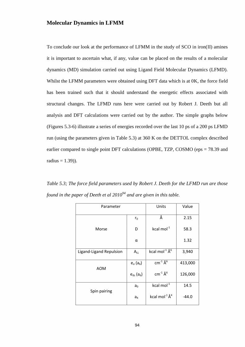
94

Molecular Dynamics in LFMM

To conclude our look at the performance of LFMM in the study of SCO in iron(II) amines

it is important to ascertain what, if any, value can be placed on the results of a molecular

dynamics (MD) simulation carried out using Ligand Field Molecular Dynamics (LFMD).

Whilst the LFMM parameters were obtained using DFT data which is at 0K, the force field

has been trained such that it should understand the energetic effects associated with

structural changes. The LFMD runs here were carried out by Robert J. Deeth but all

analysis and DFT calculations were carried out by the author. The simple graphs below

(Figures 5.3-6) illustrate a series of energies recorded over the last 10 ps of a 200 ps LFMD

run (using the parameters given in Table 5.3) at 360 K on the DETTOL complex described

earlier compared to single point DFT calculations (OPBE, TZP, COSMO (eps = 78.39 and

radius = 1.39)).

Table 5.3; The force field parameters used by Robert J. Deeth for the LFMD run are those

found in the paper of Deeth et al 201094

and are given in this table.


Morse

r0 Å 2.15

D kcal mol-1 58.3

α 1.32


AOM eσ (a6) cm-1 Å6 413,000

eds (a6) cm-1 Å6 126,000



95

The results at 360 K show clear differences between the LFMM energetics and those

obtained from single point DFT calculations (OPBE, TZP). Whilst the energetics appear

from the superposed plots to follow the same general trend the corresponding R2 is just

0.51 and 0.58 for the low and high spin states respectively. Another run this time at 220 K

had comparable results with a LS R2 of 0.56 and a HS R

2 of 0.58.

Figure 5.3; The recorded energies relative to t=0 of the last 10 ps of the LS structure at

360 K. The “correction” is a transposition by 6.23 kcal mol-1

(the average of the last 10 ps

DFT energetics, included purely for illustration).

30

35

40

45

50

55

190 191 192 193 194 195 196 197 198 199

En

erg

y r

ela

tiv

e to

t =

0 /

kca

l m

ol-1

Time / ps

DFT

LFMM

LFMM Corrected

96

Figure 5.4; The recorded energies relative to t=0 of the last 10 ps of the HS structure at

360 K. The “correction” is a transposition by 8.17 kcal mol-1

(the average of the last 10

seconds DFT energetics, included purely for illustration).



high spin LFMD run at 360K.

20

25

30

35

40

45

50

55

190 191 192 193 194 195 196 197 198 199

En

erg

y r

ela

tiv

e to

t =

0 /

kca

l m

ol-1

Time / ps

DFT

LFMM

LFMM Corrected

R² = 0.5759

20

25

30

35

40

45

50

55

35.00 40.00 45.00 50.00 55.00 60.00

DF

T E

ner

gy

Rel

ati

ve

to t

=0

/ k

cal

mo

l-1

LFMM Energy Relative to t=0 / kcal mol-1

97



low spin LFMD run at 360K.

This force field was trained to spin state splittings of complexes in local minima at 0 K. A

more accurate representation of LFMD’s ability would therefore be in its ability to track

changes in ΔEHL as a function of temperature, Table 5.6. This was achieved by taking the

difference in the average energy of the low and high spin states over the last 10 ps of the

LFMD run, Table 5.4. LFMD predicts spin crossover within the region of 220-360 K as the

sign of ΔEHL changes from positive to negative indicating a HS ground state. DFT (SPE on

LFMD structures) on the other hand destabilises the low spin state but does not favour the

HS state. Experimentally T1/2 = 335 K.17-19

This simple DFT methodology does not

reproduce experiment. It is possible that the geometrical changes during MD are even

further away from the DFT PE surface. As such the DFT energies become increasingly

unreliable. LFMD being tuned to the local minima thus gets the average behaviour as a

function of temperature correct while DFT (using LFMM structures) gets it wrong. The

test would be to perform DFT MD but this is outside the scope of this work.

R² = 0.5069

30

35

40

45

50

35.00 40.00 45.00 50.00 55.00

DF

T E

ner

gy

Rel

ati

ve

to t

=0

/ k

cal

mo

l-1

LFMM Energy Relative to t=0 / kcal mol-1

98

Table 5.4; Spin state splittings for DETTOL averaged over the last 10 ps of a 200 ps run.

ΔEHL / kcal mol-1 Error in ΔEHL

/ kcal mol-1 T / K LFMD DFT

360 -0.36 0.21 -0.57

220 1.76 2.13 -0.37

99

The construction of a mixed amine/imine force field for Fe(II)

Introduction

To date LFMM force fields for SCO applications have centred on a single ligand type i.e.

iron(II) amines. However, the majority of iron(II) spin crossover complexes include

unsaturated nitrogen donors.3 A force field capable of handling more than one ligand type

is desirable.

Training Data

Firstly in order to generate a mixed amine imine database training data is required.

Following the fact that OPBE has been shown here and by others to be reliable for iron

nitrogen systems, OPBE will also be the functional of choice for this study.

A test complex, APEFEH (Figure 5.7), was used to assess basis set effects on our chosen

systems. As can be seen in Table 5.5 the geometry of the complex is almost entirely basis

set independent with differences of < 0.01 Å in the average of all iron-nitrogen bond

lengths. The energetic effects are much starker with the SVP basis set predicting a ΔEHL of

3.05 kcal mol-1

whilst TZVP predicts a greater splitting of 7.05 kcal mol-1

. The larger

TZVP basis set (the RI approximation was utilised and so the def2-TZVP basis set was

also needed) is the basis set of choice for the remainder of this study.

100

Table 5.5: The effect of basis set on the geometry of the low and high spin states of

APEFEH with the distances given in Å. The RI approximation was utilised and so the

corresponding auxiliary basis sets were also used (def2-SVP/J and def2-TZVP/J as

appropriate).

Low Spin High Spin

AVG def2-SVP def2-TZVP Diff def2-SVP def2-TZVP Diff

Fe - N(pyr) 1.938 1.945 -0.007 2.210 2.204 0.006

N(pyr) - C 1.364 1.359 0.004 1.351 1.347 0.004

C - C 1.496 1.493 0.003 1.507 1.504 0.002

C - N 1.468 1.473 -0.005 1.460 1.465 -0.005

Fe - N 2.011 2.010 0.001 2.244 2.236 0.009

Table 5.6: The spin state splitting, ΔEHL, of the training complexes. Note that the

calculations on MELLOF07, QOQHEK and WIGPOR were carried out by Professor

Robert J. Deeth.

Refcode ΔEHL / kcal mol-1

APAFEH02146 7.1

APAFEM02147 5.2

CEYRAA148 5.7

FIWGIB149 -9.4

KEZPEK150 6.1

MELLOF07151 4.2

QOQHEK152 7.3

WIGPOR153 6.1

101

Figure 5.7; The eight pyridine/amine ligands used to form octahedral iron(II) complexes.

The database described in Figure 5.7 and Table 5.6 contains ligands with amine and

pyridine donor types, totalling 8 complexes. Initially the amine parameters kept fixed while

102

all the imine parameters were to be optimised. This assumes that force field terms are

additive i.e. the existing amine parameters will be transferable to systems in which other

ligand types are present. This mirrors the law of average environment in ligand field theory

where ligand field parameters for mixed ligand systems are estimated from adding

individual contributions from each ligand. Within fifty generations the parameter sets

generated had converged to a single Pareto front, Figure 5.8. While the errors associated

with this front are approaching reasonable values (for SCO purposes we deem errors of

less than 2 kcal mol-1

and 0.06 Å to be sufficient) they are not acceptable.

Figure 5.8; A plot of the final Pareto front of a fifty generation parameter optimisation

run. The amine parameters were kept fixed while pyridine parameters varied.

To test whether the law of average environments would apply for the LFMM parameters

some of the amine parameters were also optimised. Given that mixed ligand force fields

generate accurate structures, as demonstrated for copper(II) systems102

we focus on the

transferability of energies for SCO complexes. Since the spin state energetics are directly

related to the spin pairing term we decided to only include the pairing energy in the

1.5

2.0

2.5

3.0

3.5

4.0

0.05 0.06 0.07 0.08 0.09 0.10 0.11

En

erget

ic R

MS

D / k

cal

mol-1

Geometric RMSD / Å

103

optimisation. If the law of average environment applies then we would expect the amine

spin pairing parameters not to change.

Restarting the optimisation process results in the Pareto front shown in Figure 5.19. While

this front is superior to that from the fixed amine example, the spin pairing parameters

have changed significantly indicating the law of average environments does not apply.

The performance of the new parameters is also not as accurate as required. This may be

related to CEYRAA which is the only complex that contains pyrimidine ligands.

Removing this complex and resuming the optimisation process for two 50 generation runs

leads to the Pareto front shown in Figure 5.9. Strong energetic accuracy can only be

achieved if structural accuracy is sacrificed. Viable force fields can be obtained which

show balance in the two objectives, for instance Set 21 (an energetic error of 2.0 kcal mol-1

and a structural error of 0.062 Å) and 34 (an energetic error of 1.4 kcal mol-1

and a

structural error of 0.071 Å) tables 5.7 and 5.8 respectively. These sets were tested (Tables

5.9 and 5.10) and parameter Set 21 is chosen for its balanced treatment of both objectives.

If structural accuracy is the only goal – perhaps the generated structures are to be used as

starting points for DFT – Set 15 from the preceding run (Table 5.11) displays a geometric

RMSD of only 0.05 Å.

104

Figure 5.9: Two plots displaying Pareto Front 1 of the 50th Generation of three parameter

optimisation runs in which the amine electron pairing parameter was allowed to vary. The

first plot is across all values of the penalty functions while the second is across the region

of interest. The first optimises pyridine parameters taking the amine parameters as a

starting point (X), the second uses the same starting point excluding CEYRAA (+) and the

third takes a parameter set from the second run and further optimises it (○).

0

2

4

6

8

10

12

14

16

18

20

0.05 0.06 0.07 0.08 0.09 0.1 0.11 0.12

En

erg

etic

RM

SD

/ k

cal

mo

l-1

Geometric RMSD / Å

1

1.2

1.4

1.6

1.8

2

0.06 0.065 0.07 0.075 0.08 0.085 0.09

En

erget

ic R

MS

D / k

cal

mo

l-1

Geometric RMSD / Å

105

Table 5.7; Parameter set 21 from the second optimisation run without CEYRAA.

Parameter Units N NPYD

Morse

r0 Å 2.17 2.06

D kcal mol-1 54.9 54.9

α 1.13 1.54

Ligand-Ligand Repulsion ALL kcal mol-1 Å6 3,950 4400

AOM

eσ (a6) cm-1 Å6 416,000 547,000

eπy (a6) cm-1 Å6 - 130,000

eds (a6) cm-1 Å6 148,000 149,000

Spin pairing a0 kcal mol-1 13.5 14.9

a4 kcal mol-1 Å4 -61.4 -38.6

Table 5.8; Parameter set 34 from the second optimisation run without CEYRAA.


Morse

r0 Å 2.17 2.06

D kcal mol-1 54.9 54.9

α 1.13 1.47

Ligand-Ligand Repulsion ALL kcal mol-1 Å6 3,900 4,200

AOM

eσ (a6) cm-1 Å6 416,000 546,000

eπy (a6) cm-1 Å6 - 227,000

eds (a6) cm-1 Å6 148,000 149,000


a4 kcal mol-1 Å4 -62.0 -46.6

106


energetic RMSD and

0.0624 Å structural RMSD) of Run 2 without CEYRAA in the training set.

Name Spin State

ΔEHL / kcal mol-1 RMSD / Å

DFT LFMM M-L Heavy Atom

APAFEH02 LS 0.0 0.0 0.04 0.09

HS 7.1 10.6 0.04 0.05

APAFEM02 LS 0.0 0.0 0.03 0.15

HS 5.2 7.0 0.07 0.15

FIWGIB LS 0.0 0.0 0.08 0.14

HS -9.4 -12.7 0.03 0.15

KEZPEK LS 0.0 0.0 0.07 0.16

HS 6.1 5.9 0.02 0.31

MELLOF07 LS 0.0 0.0 0.05 0.12

HS 4.2 4.0 0.05 0.11

QOQHEK LS 0.0 0.0 0.07 0.09

HS 7.3 7.0 0.05 0.10

WIGPOR LS 0.0 0.0 0.03 0.05

HS 6.1 4.9 0.03 0.04


energetic RMSD and

0.0707 Å structural RMSD) of Run 2 without CEYRAA in the training set.

Name Spin State

ΔEHL / kcal mol-1 RMSD / Å

DFT LFMM M-L Heavy Atom

APAFEH02 LS 0.0 0.0 0.06 0.09

HS 7.1 10.2 0.04 0.05

APAFEM02 LS 0.0 0.0 0.05 0.15

HS 5.2 5.4 0.07 0.16

FIWGIB LS 0.0 0.0 0.10 0.14

HS -9.4 -10.9 0.04 0.17

KEZPEK LS 0.0 0.0 0.09 0.16

HS 6.1 5.6 0.04 0.31

MELLOF07 LS 0.0 0.0 0.07 0.13

HS 4.2 4.4 0.05 0.11

QOQHEK LS 0.0 0.0 0.09 0.10

HS 7.3 7.0 0.05 0.11

WIGPOR LS 0.0 0.0 0.05 0.05

HS 6.1 4.9 0.03 0.04

107

Table 5.11; Parameter set 15 from the first optimisation run without CEYRAA. This set is

recommended for those interested only in geometric accuracy.


Morse

r0 Å 2.17 2.10

D kcal mol-1 54.9 54.9

α 1.13 1.43

Ligand-Ligand Repulsion ALL kcal mol-1 Å6 3,950 3,080

AOM

eσ (a6) cm-1 Å6 416,000 532,000

eπy (a6) cm-1 Å6 - 51,700

eds (a6) cm-1 Å6 148,000 133,000


a4 kcal mol-1 Å4 -44.3 -70.5

108


21.


34.

The relatively poor performance of the parameter optimisation which included CEYRAA

was puzzling because the MMFF94 force field assigns the same parameter type to a

pyrimidine donor as to a pyridine donor. Hence we did not anticipate any problems.

However, the pKa for pyrimidine is substantially lower than that for pyridine, and while

previous studies have satisfactorily used a single set of parameters for ligands with

R² = 0.96

-15.0

-10.0

-5.0

0.0

5.0

10.0

15.0

-10.0 -5.0 0.0 5.0 10.0Δ

EH

L f

rom

LF

MM

/ k

cal

mol-1

ΔEHL from DFT / kcal mol-1

R² = 0.96

-15.0

-10.0

-5.0

0.0

5.0

10.0

15.0

-10.0 -5.0 0.0 5.0 10.0

ΔE

HL f

rom

LF

MM

/ k

cal

mol-1

ΔEHL from DFT / kcal mol-1

109

different pKas, e.g. primary, secondary and tertiary amines, the difference between

pyrimidine and pyridine may imply a significant enough change in metal-ligand bond

strength to warrant independent LFMM parameters for the former.

It is also clear from the parameter sets given and a comparison of the Pareto fronts that the

law of average environments does not hold true for mixed amine imine systems. Parameter

Set 21 for the mixed ligand systems gives a 10.6 kcal mol-1

energetic RMSD for the amine

training set in Figure 5.1. The behaviour for a small set of pyridine only complexes (Table

5.12) gave a smaller but still significant energetic RMSD of 5 kcal mol-1

and a geometric

RMSD of 0.09 Å. These results suggest that the law of average environments does not

apply especially for spin state energetics. This seems to correlate with the fact that the way

the spin pairing energy is handled in LFMM is qualitatively different to the other ligand

field contributions. To date the spin pairing energy was treated as being more or less

constant across different metal complexes and spin states. This assumption may be invalid

and in the future we should explore allowing the spin pairing term to be more strongly

geometry and or spin state dependant.

Table 5.12; The four complexes used as a test of the transferability of the mixed force field.

Optimised in ORCA with OPBE COSMO(water) RI def2-TZVP def2-TZVP/J

Name ΔEHL / kcal mol-1

[Fe(pyr)6]2+ -17.09

[Fe(bipy)3]2+ 15.84

fac-[Fe(6-Methyl-2,2'-bipyridine)3]2+ 1.26

mer-[Fe(6-Methyl-2,2'-bipyridine)3]2+ 5.43

110

In addition the mixed ligand parameter set requires further training data, as discussed in

Chapter 6, where it is shown how gaps in the SCO are populated. This should result in an

improved force field which is more diverse in its applications.

The use of Hammett sigma values in LFMM

The DFT study in Chapter 4 shows clearly that SCO can be influenced by substituents

attached to aromatic rings. It is intriguing to consider how such substituent effects could

possibly be incorporated in an LFMM treatment. Hammett’s work in assigning values to

these effects could prove useful as a means of quantifying variations in spin state

energetics.154

This hypothesis was tested for a series of para substituents on all six of the

pyridine rings of iron(II) tris(2,2'-bipyridine).

The DFT data was obtained using a strategy previously shown to work. The structures

were optimised using the BP86 functional70,126

and def2-SVP basis set127

with the COSMO

solvation model123,155,156

for water within the ORCA DFT package.129

The RI

approximation was used to increase speed and so an auxiliary basis set def2-SVP/J was

required. The single point energy calculations were obtained using the OPBE

functional,68,69,74,75

the TZP basis set and COSMO solvation model157

(water) within ADF

2012.01.120

The results of these calculations are shown in Table 5.13 and Figure 5.12.

111

Table 5.13; The spin-state splittings of iron(II) tris(2,2'-bipyridine) substituted on all six

para positions.

BP86 – def2-SVP OPBE – TZP

Substituent ΔEHL / kcal mol-1 ΔEHL / kcal mol-1 Hammett σ value of

a para substituent

Dimethylamino 27.15 9.94 -0.83

Amine 25.88 7.96 -0.66

Methoxy 28.08 9.20 -0.27

Ethoxy 27.93 9.17 -0.25

Methyl 30.90 12.58 -0.17

None 31.49 13.13 0.00

Fluoro 28.27 9.32 0.062

Chloro 29.67 10.77 0.227

Bromo 29.94 11.11 0.232

Iodo 30.46 11.63 0.276

Cyano 31.86 12.88 0.66

Nitro 31.73 13.18 0.778

The assumption that DFT computed values of ΔEHL would correlate with Hammett Sigma

values does not hold quite as well for these bipyridine complexes as it did for the pytacn

complexes (Chapter 4). Figure 5.12 shows the correlation of the relative DFT energetics

and the value of the Hammett σ constants. The R2 for BP86 is substantially higher at 0.68

than for OPBE at 0.48, an interesting result given that OPBE has previously been shown to

be reliable for iron(II) amine SCO complexes, as well as the fact that a larger basis set was

utilised in the OPBE energetic calculations. However, both R2 values are somewhat less

than obtained for pytacn.

112

Each pyridine ring has an ortho substituent (the other half of bipyridine) which is also

changing. This was not an issue with the pytacn systems2 studied in Chapter 4. Figure 5.12,

also appears to indicate that the unsubstituted and the para substituted methyl system are

anomalous. Interestingly H and CH3 are only inductive while the other substituents are

capable of both inductive and mesomeric effects. It is possible that while H and CH3 could

affect metal ligand σ bonding they have little effect on metal ligand π bonding while the

other substituents could affect both bonding modes. Removing H and CH3 from the plot

shown in Figure 5.12 substantially improves the R2 value to 0.91 and 0.74 for BP86 and

OPBE respectively. However, given that there are only two inductive substituents perhaps

there is insufficient data to draw meaningful conclusions from this.

Figure 5.12 – A plot of the OPBE and BP86 spin-state splittings relative to the value for

the para-amine species as a function of Hammett sigma values.

R² = 0.4804

R² = 0.6806

0

1

2

3

4

5

6

7

-1 -0.5 0 0.5 1

ΔΔ

E HL

/ kc

al m

ol-1

Hammett σp

OPBE

BP86

Linear (OPBE)

Linear (BP86)

113

Improving the Handley force field

While the parameter set in Table 5.1 is among the best achievable with the training data

given, the work of Handley and Deeth is based upon only a limited training set. Two ways

of improving upon this proof of concept work are growth of the training set to include

more varied N-Fe-N bond angles and Fe-N bond lengths as well as the inclusion of partial

charges.

The introduction of charges is vital for solid state applications which are a long term group

goal. Mulliken partial charges158

were chosen, despite their simplistic origins, as this

inclusion remains more a proof of concept than a rigorous charge scheme. The calculated

Mulliken charges for the four complexes in the Handley and Deeth paper as well as the

corresponding free ligands are given in Table 5.14. It is clear that the charges on the iron

centre vary significantly between +1.35 and +1.99 dependant on choice of ligand and spin

state of the metal centre.

114

Table 5.14; The calculated Mulliken charges for the four crystallographically

characterised complexes in the original Handley and Deeth paper. The coordinated

charges are obtained from SPE calculations (OPBE, TZP) on previously optimised

structures (BP86, RI approximation, Def2-SVP, Def2-SVP/J auxiliary basis set and

COSMO epsilon 80 refractive index 1.33 (water 80.4 and 1.33 respectively)). The

uncoordinated charges were calculated solvent free based on single point calculations

(OPBE, TZP) on the free ligands based on their LS derived structures.

Atom Uncoordinated

HS

State

Change in Charge

on Coordination

LS

State

Change in Charge

on Coordination

DETTOL Fe 2.00 1.57 -0.43 1.82 -0.18

avg N -0.25 -0.45 -0.20 -0.42 -0.22

PURYIK Fe 2.00 1.45 -0.55 1.50 -0.50

avg N -0.18 -0.32 -0.14 -0.25 -0.10

PAZXAP Fe 2.00 1.35 -0.65 1.38 -0.62

avg N -0.17 -0.40 -0.24 -0.35 -0.12

Fe399 Fe 2.00 1.57 -0.43 1.99 -0.01

avg N -0.20 -0.47 -0.27 -0.44 -0.17

This range of Mulliken charges displayed by the metal show that any model chosen to

represent them would be an inherent approximation to the “true” charges. A bond charge

increment (bond charge increments are the MMFF94 method of including charges through

polarising a bond, reducing the charge on one end and increasing it by the same amount on

the other)98

was chosen to include “Mulliken” charges in a simple manner. This is the first

time that charges have been included in an LFMM iron(II) amine force field and so even a

simple implementation is progress. Bond charge increments were derived from the iron

charges in Table 5.14 in which the average iron charge is +1.58 and so implying an iron-

115

nitrogen bond charge increment of 0.07 and so the appropriate line in the Merck derived

LFMM force field was modified. Figure 5.23 illustrates its effect on atomic charges.

Figure 5.23; The effect of the use of bond charge increments on MMFF94 charges.

This was then subjected to PROTEUS fitting. The parameter file determined as an

alternative to the Handley-Deeth parameter set was chosen as a starting point. This leads to

the initial introduction of large errors energetic RMSD of 15,836 kcal mol-1

and a

structural error of 0.39 Å. This rapidly decreases to errors of (for instance) 13 kcal mol-1

and 0.1 Å in the initial population. After two 50 generation optimisation runs, the Pareto

fronts have converged to a single front. This was taken as a sign that PROTEUS had found

the best parameter sets possible within the bounds (and bit string length) specified.

However, the energetic error was still too large at over 8 kcal mol-1

, Figure 5.24.

116

Figure 5.24; A plot of energetic RMSD against geometric RMSD for Pareto front 1 of the

50th

generation of the second parameter optimisation of a charged iron(II) amine force

field.

An alternative charge scheme lies in Deeth’s Proton Scaled Metal Ligand (PSML) charge

scheme. This charge protonates the ligand at the site of coordination in order to determine

the effect a positive charge has on the partial charges of the ligand by utilising the

MMFF94 charge scheme which deals with protonated systems.159

The charge on the proton

is that which is donated to the metal for a given spread of partial charges across the ligand.

The user determines the desired charge on the metal (from in this case natural atomic

orbital analysis,160,161

in which atomic orbitals are derived from “the one electron density

matrix”,63

Table 5.15). The script determines the metal’s proton equivalence and scales the

ligand charges appropriately. This charge scheme is superior to the BCI model above in

that it achieves the desired charge on the metal in an even manner and not simply depleting

electron density from the nitrogen. Natural charges were chosen since relative to Mulliken

charges they are more chemically “reasonable” as shown in a study on hexaqua

complexes162

in which the natural charge varied in a consistent fashion as a function of

bond length.

8

8.2

8.4

8.6

8.8

9

9.2

9.4

9.6

9.8

0.065 0.07 0.075 0.08 0.085

En

erget

ic R

MS

D /

kca

l m

ol-1

Geometric RMSD / Å

117

Figure 5.25; Top left are the charges on the nitrogen and hydrogens of ammonia and top

right the charges of protonated ammonia, NH4+. Bottom left is the charges in the transition

metal MMFF94 (without a Fe-N BCI) and right the charges under the PSML routine.

Table 5.15; The Natural Charges160,161

on iron in a range of iron(II) amine complexes as

obtained from Gaussian 03.163

HS LS

DETTOL 1.57 1.24

Fe399 1.57 1.25

PAZXAP 1.55 1.21

PURYIK 1.55 1.21

Average 1.56 1.23

This charge scheme also allows the user to more easily set spin state dependent charges on

the metals. The charge was set to +1.56 in the HS state and +1.23 in the LS state with the

ligands partial charges scaled appropriately. The force field was then refitted. The first

optimisation run of 50 generations displayed promise and a parameter set from this run

with an energetic RMSD of 1.1 kcal mol-1

and a geometric RMSD of 0.081 Å was chosen

as a starting set for a 100 generation optimisation run. This second run resulted in the

Pareto front given in Figure 5.26. Selecting a parameter set (Set 14) with similar geometric

accuracy as the uncharged force field results in a 0.2 kcal mol-1

increase in the energetic

118

RMSD from 0.9 to 1.1 kcal mol-1

. This increase is deemed acceptable. However, upon

further inspection this force field predicts the incorrect spin state for DETTOL. This

parameter set predicts it to be HS by <0.1 kcal mol-1

. Sets 4 (energetic RMSD of the whole

set 1.4 kcal mol-1

) and 10 (1.7 kcal mol-1

) likewise predict an incorrect high spin ground

state for DETTOL by 0.6 and 0.1 kcal mol-1

respectively. Set 19 recovers the correct spin

state for DETTOL predicting it to be LS by 0.7 kcal mol-1

. This parameter set has a

geometric RMSD at 0.067 Å and an energetic RMSD of 0.7 kcal mol-1

. This geometric

RMSD is slightly high. On closer inspection the highest M-L RMS is just 0.073 Å for the

HS hexamine complex, Table 5.17. While the highest heavy atom RMSD is that for HS

PURYIK, Table 5.17, at 0.18 Å. Superimposing the two complexes with the highest heavy

atom RMSD (Figure 5.27) reveals that the structural deviations are acceptable given the

high energetic accuracy (an RMSD of 0.7 kcal mol-1

) of the force field. Therefore, since

the structural RMSD, considering iron-nitrogen and nitrogen-nitrogen distances is less than

0.07 and the structures of the two complexes with the largest heavy atom RMSDs are still

qualitatively correct this force field (Parameter Set 19) is the one recommended for use.

119

Figure 5.26; A plot of Pareto front 1 from the 100th

generation of the second parameter

optimisation run.

0.5

1

1.5

2

2.5

0.055 0.057 0.059 0.061 0.063 0.065 0.067 0.069 0.071

En

erget

ic R

MS

D /

kca

l m

ol-1

Geometric RMSD / Å

120

Table 5.16; Parameter set 19 from Figure 5.26, with an energetic RMSD of 0.73 kcal mol-1

and a geometric RMSD of 0.067 Å.


Morse

r0 Å 2.22

D kcal mol-1 54.9

α 1.26


AOM eσ (a6) cm-1 Å6 412,000

eds (a6) cm-1 Å6 118,000



Table 5.17; The metal-ligand and heavy atom RMSDs for the iron(II) amine training set

when using parameter set 19. Distances in Å.

Identifier Spin State M-L Heavy Atom

[Fe(NH3)6]2+ HS 0.07 0.08

[Fe(NH3)6]2+ LS 0.01 0.01

PURYIK HS 0.06 0.18

PURYIK LS 0.03 0.09

DETTOL HS 0.03 0.07

DETTOL LS 0.02 0.08

PAZXAP HS 0.05 0.13

PAZXAP LS 0.01 0.09

FE399 HS 0.01 0.13

FE399 LS 0.01 0.05

121

Figure 5.27; A superposition of the two complexes with the highest heavy atom RMSD for

Parameter Set 19. HS PAZXAP is shown on the left with a heavy atom RMSD of 0.13 Å.

Right is HS PURYIK with a heavy atom RMSD of 0.18 Å.

Generating a charge scheme in MM is both critical and challenging.164

Utilisation of the

normal Coulombic expression to partial atomic charges as in Equation 5.1 introduces long

range interactions which would otherwise be screened in real systems.

𝐸 =q𝑖q𝑖

𝜀𝑟 Equation 5.1

Various methods have been developed to reduce these long range interactions. The

distance dependent dielectric, which is utilised here, is based upon a modification of

Equation 5.1 to depend on the square of inter atomic distances. While there is no guarantee

that partial atomic charges derived from DFT calculations are appropriate for molecular

mechanics. It has been shown here that these charges can be included within a force field

and the parameters optimised around it. This resulted in a parameter set with similar

accuracy to the uncharged force field discussed at the start of the chapter. The use of

122

Deeth’s Proton Scaled Metal Ligand charge scheme could prove invaluable for the

inclusion of charges in to systems for which the spin state independent BCI scheme fails.

Addressing the stiff iron-nitrogen-carbon angle term

Within the Handley-Deeth force field the iron(II)-nitrogen-carbon bond angle has a force

constant of 200 kcal mol-1

deg-2

(and a reference angle of 115°) compared to the generic

M+2

-N-C angle having a force constant of just 30 kcal mol-1

deg-2

. No reports were made in

previous publications as to the reason for this. Using a parameter set (Table 5.18) which

reported an energetic RMSD of 0.24 kcal mol-1

and a geometric RMSD of 0.065 Å (force

constant of 200 kcal mol-1

deg-2

) as a starting point the force constant was reduced to

30 kcal mol-1

deg-2

. This reduction in force constant resulted in an energetic RMSD

2.75 kcal mol-1

and a geometric RMSD of 0.060 Å. While this adjustment slightly

improves upon the geometric term, it is well within the range of those generated in

preceding optimisation runs and is not proportionate to the > 2.5 kcal mol-1

reduction in the

energetic term.

123

Table 5.18; The parameter set for which an energetic RMSD of 0.24 kcal mol-1

and a

geometric RMSD of 0.065 Å is obtained using the Fe+2

-N-C force constant of

200 kcal mol-1

deg-2

.


Morse

r0 Å 2.18

D kcal mol-1 49.5

α 1.13


AOM eσ (a6) cm-1 Å6 412,000

eds (a6) cm-1 Å6 143,000



Table 5.19; The energetic and geometric data obtained after altering the iron(II)-N-C

force constant from 200 to 30 kcal mol-1

deg-2

.

Refcode Spin State

ΔEHL / kcal mol-1 M-L RMSD / Å

Heavy Atom RMSD / Å DFT LFMM

[Fe(NH3)6]2+ HS -6.7 -6.3 0.060 0.058

LS

0.025 0.024

PURYIK HS -1.6 -1.2 0.029 0.080

LS 0.038 0.065

DETTOL HS 1.5 -3.3 0.036 0.092

LS 0.034 0.050

PAZXAP HS 14.4 11.0 0.020 0.078

LS 0.022 0.061

FE399 HS 1.6 3.2 0.032 0.177

LS 0.001 0.065

As can be seen in Table 5.19 the largest energetic errors correspond to DETTOL and

PAZXAP. DETTOL is predicted to have a HS ground state using this parameter set and

not the low spin state shown by experiment.

124

Figure 5.28; The final Pareto front of the fifty generation optimisation run with a reduced

bond angle force constant.

After a fifty generation optimisation run the lowest energetic RMSD obtained was 2.33

kcal mol-1

, which is substantially larger than the 0.24 kcal mol-1

RMSD obtained with the

stiffer force constant. In the light of this result it may be worthwhile reviewing previously

developed force fields to see whether increasing the angle bend force constants at the

donor atom would be beneficial.

2.3

2.4

2.5

2.6

2.7

2.8

2.9

3

0.04 0.045 0.05 0.055 0.06 0.065E

ner

get

ic R

MS

D /

kca

l m

ol-1

Geometric RMSD / Å

125

Increasing the Transferability

Since the force field was not trained with aromatics in mind (despite their chemical

interest) it was deemed prudent to test its transferability before it could be used. The simple

tris(1,2-diaminobenzene) iron(II) complex, Figure 5.29, was chosen.165

This complex

displays bending of the benzene rings out of the plane of the Fe-N-C bond angle as shown

in Figure 5.29 which shows the HS crystal structure (χMT300K = 3.96 emu K mol−1

).165

Figure 5.29; The HS crystal structure of tris(1,2-diaminobenzene) iron(II)165

DFT corroborates this distortion in the Fe-N-C angle which is more pronounced in the high

spin than the low spin state due to the weaker bonds to the metal and reduced steric

crowding.

An uncoordinated 1,2-diamino benzene molecule is a conjugated system in which the lone

pairs on the nitrogen are involved in bonding with the ring. As a result the geometry at the

uncoordinated nitrogen is not a trigonal pyramidal sp3 hybrid but is instead a trigonal

planar sp2 hybrid with the unpaired electron lying perpendicular to the plane of the

nitrogen, Figure 5.30.

126

Figure 5.30; The direction of the nitrogen p-orbital containing the lone pair in

uncoordinated amino benzene.

In contrast the standard MMFF94 N atom type presumes the nitrogen is tetrahedrally

coordinated which means that the Fe-N-C plane and the H-N-H plane are orthogonal and

the Fe lies in the plane of the ligand. The true coordination lies between these two

extremes. Within MOE as in MMFF9498

torsions are treated as a Fourier series. This series

consists of five cosine functions (MMFF94 uses three terms) Equation 5.2 and through

varying the Vn constants the profile of the torsional potential energy surface can be tuned.

𝐸𝑡𝑜𝑟𝑠(𝜔) = 1

2(𝑉1(1 + cos(𝜔)) − 𝑉2(1 − cos(2𝜔)) + 𝑉3(1 + cos(3𝜔)) − (𝑉4(1 −

cos(4𝜔)) + 𝑉5(1 + cos(5𝜔)) Equation 5.2

127

Figure 5.31; A plot of 1+cos(2x) to illustrate the second term scaled by V2/2.

Using a systematic approach the force constant was varied to reproduce the DFT generated

structures. Values of the first three Vn/2 force constants were varied, Figure 5.32, and it

was found that the lowest structural error (heavy atom RMSD) comes from setting V2/2 to

1.75. So this becomes the recommended value for use in LFMM calculations on amino

benzenes. Figure 5.33 illustrates the overlap of the crystal165

and high spin LFMM

structures of [Fe(1,2-diaminobenzene)3]2+

. While the overlap is not total it is a noticeable

improvement on the default value. Should 1,2-diaminobenzene complexes be of interest

for SCO applications it is recommended that a force field refitting takes place to achieve

the desired energetic accuracy for these systems.

128

Figure 5.32; Plots of the effect of varying the torsional constants V1/2, V2/2 and V3/2 on

the heavy atom RMSD of LFMM structures from the DFT reference structures.

0

0.2

0.4

0.6

0.8

1

1.2

1.4

-4 -2 0 2 4

Hea

vy A

tom

RM

SD

/ Å

V1/2

LS

HS

0

0.2

0.4

0.6

0.8

1

1.2

1.4

-4 -2 0 2 4

Hea

vy A

tom

RM

SD

/ Å

V2 / 2

LS

HS

0.00

0.20

0.40

0.60

0.80

1.00

1.20

1.40

-15 -10 -5 0 5 10 15

Hea

vy A

tom

RM

SD

/ Å

V3 / 2

LS

HS

129

Figure 5.33; The overlap of the crystal structure165

and the high spin LFMM structure

using the new Fe-N-Car-Car torsional force constant.

130

Chapter 6 – The Design of Novel Transition Metal Complexes

through Ligand Generation

Despite the volume of iron(II) SCO research published in recent years few groups have

pursued the same goal for cobalt(II) systems. Cobalt(II) is d7 and can therefore adopt either

a low (2E) or high (

4T1) spin form, in octahedral symmetry, involving 1 or 3 unpaired

electrons respectively. This is classically illustrated in the form of a Tanabe-Sugano

diagram as in Figure 6.1. With studies and reviews in general (see Chapter 1) focussing on

unsaturated ligands for six coordinate species50

no LFMM studies have focussed on

cobalt(II) systems either four or six coordinate.

Figure 6.1; The d7 Tanabe-Sugano diagram.

13 CoIII refers to Co

2+ and F specifies triply

orbitally degenerate octahedral terms. Reproduced with permission from the Physical

Society of Japan.

131

A search of the Cambridge Structural Database reveals that four coordinate cobalt (II)

amine complexes do indeed span the spin crossover divide. This is evidenced by the fact

that both square planar (LS) and tetrahedral (HS) complexes are contained within the

database. The d-orbital splittings for the LS and HS complexes are shown in Figure 6.2.

Figure 6.2; The d-orbital splittings of 4-coordinate cobalt(II) amine complexes. The low-

spin square planar complex is depicted on the left and the high-spin tetrahedral complex is

depicted on the right.

Somewhere between planar and tetrahedral geometries must lie the SCO region. To

discover this region an automated procedure will be utilised. Using the drug discovery

tools in MOE, ligands can be designed “from scratch”. Users input a simple scaffold and

from it a range of potential ligands are generated. From these ligands, candidates for SCO

are determined and fine tuning of the SCO energy can be carried out. The user can select

points of likely substitution and watch as the tools output candidates around the SCO

divide (as well as many outside of it). These candidates are then verified by Kohn-Sham

density functional theory.

132

The parameterisation of a robust cobalt(II) force field

The term robust, as used in the title, is of key importance. This force field needs to be

capable of handling both the high- and low-spin states as well as tetrahedral and square

planar geometries. The subtle balance between the two, which is achieved here, is

something molecular mechanics had in the past struggled with; that is, before the inclusion

of explicit ligand field effects.

Cobalt(II) amine force fields have long been a goal of our research group. However, the

work that had been carried out on these systems by Summer and Masters students had only

limited success. The work reported here represents the first utilisable cobalt(II) amine force

field.

Computational Details

Structures were optimised using the BP86 functional,70,126

the RI approximation, the def2-

SVP basis set127

and the COSMO solvation model (water) within the ORCA package.

Initially Version 2.9.1 of the ORCA code was used followed by Version 3.0.1.129

Since no

difference is expected in the structures predicted by these implementations distinctions will

not be made in the body of the text. Energetics were determined through single point

calculations within ADF 2012.01120

using the OPBE functional,74,141

TZP basis set,142

COSMO123

(water, dielectric constant = 78.39, radius = 1.93 Å) and the SCF sub keys of

mixing and level shifting were set to 0.1 and 0.3 respectively. This methodology does not

include all of the corrections reported to “improve” calculations including dispersion, zero-

point corrections, entropy and relativistic effects as these have been shown in Chapter 4 to

reduce agreement with experiment in spite of their notional improved theoretical

grounding. Ligand Field Molecular Mechanics calculations were carried using

133

DommiMOE101

within Molecular Operating Environment 2010.10144

and 2011.10.145

The PROTEUS automated parameterisation tool,1 described in Chapters 3 and 5, was

employed for all parameters apart from the angular overlap model (AOM) e parameters

which were determined, and then fixed, using the following procedure.1 The AOM

parameters are derived by fitting the energies of the predominantly d molecular orbitals

from DFT calculations. The DFT orbital populations are averaged to generate an

approximate spherical potential to mimic ligand field theory.166

(ADF single point

calculations, OPBE, TZP with small cores and set occupancies of 1.4 in each d-orbital on

cobalt(II) bis-ethylenediamine and cobalt(II) tetramine.)

In a square planar geometry, as adopted by LS four coordinate cobalt(II) species, the d-

orbitals can be expressed in terms of eσ and eπ as follows;

𝐸(𝑥2– 𝑦2) = 3𝑒𝜎

𝐸(𝑧2) = 𝑒𝜎 − 4𝑒𝑑𝑠

𝐸(𝑥𝑧, 𝑦𝑧) = 2𝑒𝜋

𝐸(𝑥𝑦) = 4𝑒𝜋

Since amines are not π-donors the xz, yz and 𝑥𝑦 orbitals are degenerate. Analysis of the d-

orbital composition of the LS bis-ethylenediamine complex is given in Table 6.1. (Note

that the axis alignment here has the x and y axes bisecting the N-Co-N angle, effectively

interchanging the xy and 𝑥2– 𝑦2 orbitals). This leads to an eσ of 9375 cm-1

and an eds of

2074 cm-1

for this LS complex.

134

Figure 6.3; Axis frame definition for low spin cobalt(II) bis-ethylenediamine.

Table 6.1; The energies of the LS molecular orbitals of cobalt(II) bis-ethylenediamine and

the contributions of the atomic d-orbitals

Orbital

Energy /eV

d-orbitals and % contributions

to the molecular orbitals

Total % d orbital

contribution

-6.656 xz 96% 96%

-6.574 yz 96% 96%

-6.377 z2 60% 87%

x2-y2 27%

-6.303 x2-y2 67% 89%

z2 22%

-3.024 xy 57% 57%

135

Table 6.2; The energies of the HS molecular orbitals of cobalt(II) bis-ethylenediamine and

the contributions of the atomic d-orbitals

Orbital Energy /eV

d-orbitals and % contributions to the molecular orbitals

Total % d orbital contribution

-6.500 x2-y2 77% 97%

yz 10%

xy 6%

xz 3%

-6.369 z2 59% 93%

xz 18%

yz 14%

xy 1%

-5.913 xy 61% 75%

xz 7%

x2-y2 5%

yz 2%

-5.238 yz 46% 69%

z2 14%

xy 6%

x2-y2 3%

-5.216 xz 47% 68%

z2 10%

x2-y2 6%

yz 3%

xy 3%

The HS orbitals can be described in terms of e parameters as follows;

𝐸(𝑥𝑧, 𝑦𝑧, 𝑥2– 𝑦2) = (4

3) 𝑒𝜎 + (

8

9) 𝑒𝜋

𝐸(𝑧2, 𝑥𝑦) = (8

3) 𝑒𝜋

This results in an eσ of 5921 cm-1

for the HS bis-ethylenediamine complex. A similar

analysis was carried out on the analogous tetramine complex with the eσ values reported in

Table 6.3. The AOM parameters are implemented in DommiMOE as a function of metal

136

ligand bond length as described in Chapter 3. Assuming a sixth order dependence and

reducing the sum of the percentage errors results in an a6 term of 481,234. This will be

rounded to 481,000 for implementation. An a6 term was utilised as this results in a smaller

error than an a5 term with a mean absolute percentage error of 10 vs 12%. While use of

several en parameters would allow an exact fit to DFT it will greatly increase the number of

parameters and so a compromise was made. Similarly assuming a 6th

order dependence of

the d-s mixing term on the bond length results in an a6 of 119,908 which was rounded to

120,000.

Table 6.3; Values of eσ as derived from DFT calculations and the error through deriving

them from an a6 of 481,234 cm-1

Å-6

.

Spin

State

Average

Co-N Bond

Length / Å

DFT Derived

𝑒𝜎 / cm-1

𝑒𝜎 / cm-1 as derived

from an a6 of

481,234/ cm-1 Å6

% Error

Cobalt(II) bis-

ethylenediamine

LS 1.96 9375 8410 -10.3

HS 2.05 5921 6505 9.9

Cobalt(II)tetramine LS 1.96 9297 8455 -9.1

HS 2.04 6045 6620 9.5

Sum of % errors 0

This force field employs a simple charge model based on the change in Mulliken charges

from DFT calculations on high and low spin calculations on the bis-ethylenediamine

species to obtain an average iron(II)-N bond charge increment of 0.26 which was

subsequently added to the force field file.

137

Table 6.4; The derivation of the bond charge increment for use in the LFMM force field.

Atom Type

MMFF_tm Free

Ligand Charge on the

HS species Charge on the

LS species Average Change in

Charge

Co 2.00

1.01 0.87 -1.06

N -0.99 -0.37 -0.33 -0.29 0.06

HN 0.36 0.09 0.15 0.15 0.06

C 0.27 0.39 0.40 0.41 0.01

HC 0.00 -0.10 -0.06 -0.07 0.04

The ligand builder and attachment routines reported here form a novel route to spin-

crossover complexes. It allows the user to input simple bidentate ligands, for instance

ethylenediamine or propylenediamine, and replace part of the “scaffold” (carbon backbone

in these cases) with entries in an R-group library. This is termed Scaffold Replacement

within MOE. It is also possible to replace hydrogens on the ligand with entries in this

library; this is known as R-group addition. These two strategies allow the generation of

thousands of possible ligands. Combinatorial strategies do not claim to sample all ligands.

Rather it is hoped instead that a diverse enough subset of all ligands will be sampled in

order to assess the viability of a given coordination sphere to display SCO. Examples of

the type of ligands generated will be shown in the coming sections.

All candidates were subjected to a rigorous routine of stochastic conformational searching.

The stochastic conformational search routine implemented in DommiMOE is based on the

work of Ferguson and Ramer.167

The routine is based upon random perturbations in the

ligands torsion angles within pre-set bounds. As a result, the unrestrained metal ligand

bond lengths are allowed to vary greatly and therefore sampling is a direct product of

torsional perturbations. One spin-state structure needs to be optimised first, the choice of

which is arbitrary. This routine optimises the HS state first followed by the LS state as per

Figure 6.4. To ensure that as few false negatives are removed as possible candidates with

small negative values of ΔEHL needed to pass through the initial cut-offs. This would allow

candidates the opportunity to return to the SCO region in subsequent searches.

138

Figure 6.4; Illustrating the effect of the order in which the stochastic searching is carried

out and its relationship with “predicted” spin state energetics.

All ligands proposed have been determined to be 100% synthesisable by MOEs internal

retrosynthetic analysis tool which breaks down molecules in to their precursors and

compares these to a database. If all of the precursors are contained in the database then the

molecule is said to be synthesisable as described in the MOE documentation.

139

Results and Discussion

Five cobalt(II) complexes with tetradentate amine donors based on 14 and 16 membered

rings have been synthesised and are reported in the literature. Three of these complexes,

NENCEO,168

RUJSEU169

and QORPOC170

(the sixteen membered rings depicted in Figure

6.5) are high spin whilst COANEC171

and TEXQIW172

(fourteen membered rings) are low

spin. However, no spin crossover systems have been reported. This force field once

developed will allow users to populate the SCO window with potential SCO complexes.

Figure 6.5; The five macrocyclic systems which have been reported in the literature and

their Cambridge Structural Database refcodes.

A force field trained on just five complexes is possible. However, it might lack the

diversity necessary for the subsequent high throughput screening. More training data are

probably required. The DFT methodology (BP86 with solvation for structures and OPBE

140

with solvation for energetics the standard protocol as described in Chapter 4) was validated

against the five macrocyclic complexes (Figure 6.5) for which crystal structures have been

reported.

Table 6.5; A comparison of the crystal structures of five cobalt(II) tetramine complexes

and the DFT optimised structures.

Refcode Ground State Av. Co-N Bond

Length / Å

Bond Angle / °

1 2 3 4 5 6

COANEC LS Expt 1.98 180.0 180.0 94.1 94.1 85.9 85.9

DFT 1.99 180.0 180.0 93.8 93.8 86.2 86.2

NENCEO HS Expt 1.99 130.4 115.8 105.6 104.9 101.2 99.9

DFT 2.03 129.0 117.1 105.2 105.1 100.9 100.8

QORPOC HS Expt 2.02 126.2 107.8 107.2 104.8 104.6 104.3

DFT 2.02 121.1 107.2 106.8 107.1 106.7 107.2

RUJSEU HS Expt 2.01 124.6 122.9 106.0 104.9 101.4 98.9

DFT 2.03 123.9 123.8 102.8 102.8 102.8 102.8

TEXQIW LS Expt 2.01 180.0 180.0 94.2 94.2 85.8 85.8

DFT 2.00 180.0 180.0 93.8 93.7 86.2 86.2

To provide more training data, calculations on generated complexes were carried out to

help fill out the energetic region between the 14 and 16 membered rings, as well as to

provide more diverse structures for the training. For the purposes of generating training

data, the structures generated need not be global minima only local. The additional

complexes are shown in Figure 6.6 as well as cobalt(II) bis-ethylenediamine (C1). The

energetics of extended training set are given in Table 6.5.

141

Figure 6.6; The complexes added to the training set in Figure 6.4 to give Training Set 1

(T1).

142

Table 6.6; The complexes in training set, T1, denoted by their CSD refcodes or designation

from Figure 6.5.

ΔEHL / kcal mol-1

COANEC 18.54

TEXQIW 17.56

C2 10.70

C1 6.80

C3 2.17

C5 -0.70

C4 -4.80

NENCEO -11.29

RUJSEU -12.29

QORPOC -17.16

A fifty generation parameter optimisation run was carried out allowing all (excluding

AOM) parameters to vary. The final Pareto front is shown in Figure 6.7 and the chosen

parameter set in Table 6.7 which shows balance in the two objectives. The performance of

this parameter set is illustrated in Figure 6.8.

143

Figure 6.7; The final Pareto front of the fifty generation parameter optimisation run

training set (T1).

Table 6.7; Parameter set 3 (P1S3) from the Pareto front given in Figure 6.7. A parameter

set which shows balance in the two objectives for the training set given in figures 6.5 and

6.6.


Morse

r0 Å 2.09

D kcal mol-1 60.0

α 1.40


AOM eσ (a6) cm-1 Å6 481,000

eds (a6) cm-1 Å6 120,000


a6 kcal mol-1 Å6 338

1.75

1.80

1.85

1.90

1.95

2.00

2.05

0.0535 0.0540 0.0545 0.0550 0.0555 0.0560 0.0565 0.0570

En

erget

ic R

MS

D /

kca

l m

ol-1

Geometric RMSD / Å

144

Figure 6.8; A plot of ΔEHL values obtained from LFMM (P1S3) against the DFT target

value for training set, T1.

Using the ligand generator routines the CC scaffold of the ethylenediamine ligand was

selected for replacement. Of the bis-bidentate complexes generated, 102 lie within our

window of interest (EHL 6 to -2 kcal mol-1

) based upon LFMM energetics. This simple

validation is not yet looking for a global minimum and as such a full conformational search

is not required. Of the 102 complexes, 25 were predicted to be synthesisable.

Synthesisability was determined using MOE’s rsynth tool. An rsynth of 1 (a measure of

synthesisability based on retrosynthetic analysis) suggests the molecule is synthesisable

while a value of 0 suggests it cannot be made. Values in between indicate varying

likelihoods of successful synthesis. Three complexes were chosen to test the current

parameter set (Figure 6.9).

R² = 0.98

-20

-15

-10

-5

0

5

10

15

20

-20 -15 -10 -5 0 5 10 15 20Δ

E HL (L

FM

M)

/ k

cal

mo

l-1

ΔEHL (DFT) / kcal mol-1

145

Figure 6.9 – The three cobalt(II) tetramine complexes with bidentate ligands selected for

initial validation of P1S3.

Table 6.8 – The energetics of the small validation set, energies given in kcal mol-1

LFMM DFT

Complex ΔEH-L HS LS ΔEH-L Error

1 5.21 -3730.6 -3728.63 5.63 0.42

5 4.42 -4487.17 -4492.65 5.48 1.06

22 2.74 -5222.94 -5225.2 2.26 -0.48

To provide further training data complexes 1 and 5 (22 excluded as error was small) were

folded in to the training set to give training set (T2). Whilst these complexes are similar to

each other, the subtle differences in the coordination environment (the ΔEHL values of 1

and 5 are only 0.15 kcal mol-1

different in energy yet LFMM predicted a difference of 0.79

kcal mol-1

) provide a further test. Whilst the overall RMSD energetic error fell to 1.7 kcal

mol-1

the RMSD of the complexes already in the set fell only by 0.04 kcal mol-1

; an

inconsequential amount. The errors of the new training set fell (by 0.81 kcal mol-1

for

146

complex 5) showing that their inclusion did improve upon the initial force field. As

expected this inclusion offers no improvement for those complexes already in the set.

Table 6.9; Parameter Set 13 (P2S13) from the optimisation on training set, T2.


Morse

r0 Å 2.09

D kcal mol-1 60.0

α 1.47


AOM eσ (a6) cm-1 Å6 481,000

eds (a6) cm-1 Å6 120,000



147

Table 6.10: The energetic errors for Par File 13, P2S13, from the first optimisation run on

Training Set 2, T2.

Identifier ΔEHL (DFT)

/ kcal mol-1

ΔEHL (LFMM)

/ kcal mol-1

Error

/ kcal mol-1

COANEC 18.54 16.80 -1.74

TEXQIW 17.56 14.57 -2.99

C2 10.70 9.81 -0.89

C1 6.80 6.37 -0.43

1 5.63 6.05 0.42

5 5.48 5.73 0.25

C3 2.17 4.09 1.92

C5 -0.70 -1.39 -0.69

C4 -4.80 -2.99 1.81

NENCEO -11.29 -9.47 1.82

RUJSEU -12.29 -9.81 2.48

QORPOC -17.16 -19.33 -2.17

148

Figure 6.10; The correlation of DFT and LFMM computed ΔEHL (kcal mol-1

) using the

parameter set given in Table 6.9 on T2.

It is clear from Table 6.10 that whilst the parameterisation for four coordinate species is

sound (R2 =0.98, Figure 6.10) there is a slight anomaly. Despite the fact that the

QOPRPOC error is lower than those of TEXQIW and RUJSEU the sign of the error

remains the issue. The error for QORPOC is of the opposite sign to those in the lower left

quadrant of Figure 6.10 and experimenting with its removal, leads to a reparametisation

which offers lower errors in both objectives, Figure 6.11. While the removal is not

reasonable,‡ it did highlight a deficiency in the FF which should be addressed. QORPOC is

a sixteen membered chelate with a propane tether connecting two opposite nitrogens. It is

comprised entirely of 6 membered rings; these have been shown to be an issue for the

iron(II) amine systems studied by Deeth and Handley (2011) as in six membered rings

there are two torsion terms involving the Fe-N bonds which are assigned zero force

constants.1 Consequently the chelate ring is unable to adopt all the various conformations

found for six membered rings. They solved this problem by explicitly tuning the Fe-N-C-C

‡ A truly diverse force field should be capable of handling all related systems. As such the

removal of a structure which has been crystallographically observed is deemed to be

unreasonable.

R² = 0.98

-25

-20

-15

-10

-5

0

5

10

15

20

-20 -15 -10 -5 0 5 10 15 20

Pre

dic

ted

ΔE

HL f

rom

LF

MM

Predicted ΔEHL from DFT

← QORPOC

149

torsion term rather than simply relying on the default generic *-N-C-* (* represents any

atom) entry in the MOE force field. The introduction of a similar term here (using the

parameters used in the iron example as a starting point) resulted in an improved description

of the QORPOC energetics leading to a fall in energetic error from 1.27 kcal mol-1

to 0.90

kcal mol-1

. This reduction in error comes at a high cost, greatly increasing the errors

associated with some of the other systems in the set.

One possible solution is an on the fly identification of six membered rings and thus a

different treatment of them w.r.t their five membered counterparts. However it remains

unclear as to whether this is the root cause of the issue. Another unique point to note being

that both QORPOC and the C5 species are the only complexes containing tertiary amine

donors. Perhaps the use of different parameters for primary, secondary and tertiary amines

would improve the fit. These extra levels of complexity are unlikely to prove worthwhile

as despite the fact that the C5 complex shares many of the characteristics of QORPOC

(other than one carbon in a chelate ring) the performance of the force field is markedly

different with a 1.48 kcal mol-1

lower error in the predicted ΔEHL of C5 than that of

QORPOC.

Figure 6.11; Final Pareto fronts with and without QORPOC in the training set.

1.05

1.15

1.25

1.35

1.45

1.55

1.65

1.75

1.85

0.047 0.052 0.057 0.062

En

erg

etic

RM

SD

/ k

cal

mo

l-1

Geometric RMSD / Å

With QORPOC

Without QORPOC

150

True high throughput screening

Bidentate Ligands

After running scaffold replacement and R-group addition routines, using the groups given

in Figure 6.12, 349 bidentate nitrogen donating ligands were created based upon

ethylenediamine and propylenediamine. Of these, 67 entries had an rsynth of 1, this

retrosynthetic analysis tool is outlined further in the Computational Details section of this

chapter. These 67 ligands were attached to the metal following the procedure outlined in

Appendix 2 forming 67 bis-bidentate complexes. These candidates were subjected to

rigorous stochastic conformational searching, first for 2000 steps and then for 4000 steps

(chiral restraints were used as both enantiomers will be contained in the database for many

of the complexes). If both searches result in a best structure with same energy then it is

assumed that this is the lowest energy conformation possible for this complex. From this

search only one (if any) of the bis-bidentate complexes offers a likely candidate for SCO.

This may be an indication of the need to lock potential SCO candidates into a metal

geometry between tetrahedral and square planar.

151

Figure 6.12; The R-groups used for addition and replacement on ethylene diamine and

propylene diamine ligands. CH4 and C2H6 were also included in the R-group library

however these (most likely due to MOEs internal rules) do not participate in R-group

addition.

152

Figure 6.13; The bis-bidentate complexes ordered by ΔEHL. The blue dashes denote the

splitting after 2000 steps of stochastic conformational searching (at the HS state) whilst

the red crosses denote 4000 steps. The oval indicates the absence of complexes in the SCO

region.

It is, in the case of bidentates, too easy for them to fall in to their preferred geometry. It is

believed that those complexes with secondary amine donors must adopt a tetrahedral

ground state in order to reduce steric interactions between ligand groups, figures 6.13 and

6.14. However, those complexes with only primary amine donors can adopt either a square

planar or tetrahedral geometry dependent on the nature of the ligand. For instance the bis-

propylenediamine complex and all of its carbon substituted derivatives studied have larger

bite angles and are tetrahedral whilst the bis-ethylenediamine complex and its derivatives

are low spin consistent with a smaller bite angle and lower steric interactions. This mirrors

the relationship between the size of the macrocycle and ground spin state in the literature.

-15

-10

-5

0

5

10

0 10 20 30 40 50 60 70

LF

MM

Pre

dic

ted

ΔE

HL/

kca

l m

ol-1

Potential SCO Complex

153

Figure 6.14; Three representative examples of ligands in the bidentate database along

with their LFMM predicted (P2S13) value of ΔEHL

Hence with bidentate nitrogen ligands it is difficult, if not impossible, for four-coordinate

cobalt(II) to display SCO. The only bidentate complex predicted by LFMM to display SCO

is that formed from 1,2-diaminobenzene ligands as in Figure 6.15. However, upon DFT

optimisation the structure distorts Figures 6.16 and 6.17 and the DFT predicted spin state

splitting is larger than predicted by LFMM at 7 kcal mol-1

. As subsequently discovered for

iron complexes, and reported in Chapter 5 the aniline type nitrogen is planar when

uncoordinated but the force field parameter type enforces a tetrahedral coordination. This

problem can be corrected but given that the bidentate systems are not good candidates for

SCO this was deemed unnecessary.

154

Figure 6.15; The only complex with bidentate ligands predicted to display spin crossover.

Figure 6.16; The distorted tetrahedral structure obtained upon DFT optimisation of high

spin [Co(1,2-diaminobenzene)]2+

.

Figure 6.17; The distorted structure obtained upon DFT optimisation of low spin [Co(1,2-

diaminobenzene)]2+

.

155

Tetradentate Ligands

To form tetradentate complexes, eight of the bidentate ligands previously generated

(depicted in Figure 6.18) were used as the starting ligands and the R-group addition tool

used upon them to generate tetradentates. This is to say that linking occurred, with the 8

bidentate starting points bonded to the whole database of 349 bidentate ligands. Ligands

L1-L5 had all hydrogens selected as points for potential substitution whilst L6-L8 only the

hydrogens which are inside the dashed lines in Figure 6.18 could be replaced. Filters were

used to remove nitrogen-nitrogen single and double bonds as well as nitrogen-carbon

double bonds as such systems fall outside the scope of this study.

Figure 6.18; The bidentate ligands chosen for ligand growth. Ligands L1-L5 had all

hydrogens selected as points for potential substitution whilst L6-L8 only the selected

hydrogens could be replaced.

156

The eight ligand starting points were carefully selected. L1 and L2 represent simple

systems upon which the complexity arises simply from the ligands to which they are

bonded. This generated 249 and 8,937 unique ligands respectively. Ligands L3-L8

introduce substituents whose effects may be felt. The reason for the inclusion only of those

hydrogens within the dashed line is a pragmatic one. The inclusion of all of the hydrogens

of ligands L6-L8 resulted in the program crashing as a result of insufficient memory.

Of the over one hundred thousand (103,944) unique ligands generated, MOE’s internal

retrosynthetic tool predicted 4,347 of these to be synthesisable. The ligands deemed

synthesisable were then attached to the metal using a ligand attachment script. The

selection of this much reduced subset greatly reduced the computational cost allowing the

subsequent stochastic searching to be carried out on a local machine over the course of

days rather than months and increases the chances that predicted SCO complexes have

ligands which are synthesisable.

Of these synthesisable candidates generated, 366 potential SCO complexes based on linear

or branched tetradentates (excluding those with four membered chelates) have a spin state

splitting of between 0 and 5 kcal mol-1

. Preliminary stochastic searching (2000 steps

representing close to 2 million individual geometry optimisations) on those complexes

with values of ΔEHL initially predicted to be between +10 and -5 kcal mol-1

(983

complexes) narrowed this number slightly to 349 (322 from entries originally predicted in

this range). The candidates for SCO are discussed in depth later as they share

characteristics with the macrocyclic systems.

157

Figure 6.19; A plot of all linear and branched candidates based on raw data i.e. the

structures have undergone only a small stochastic search.

-10

-5

0

5

10

0 500 1000 1500 2000 2500 3000 3500

Sp

in S

tate

Sp

litt

ing

E(H

S-L

S)

/ k

cal

mo

l-1

Potential SCO Complex

158

Macrocycles

Macrocyclic ligands are generated through a SMARTS§ match based routine which

identifies a chain and subsequently bridges it with either a two or three membered carbon

linker, Figure 6.20. These ligands were subjected to a near identical screening process to

that used for the tetradentates.

Figure 6.20; An illustration of the identification of a backbone capable of supporting

macrocycle formation and the joining to form it.

Unfortunately DFT validation of LFMM energetics resulted in unacceptably large

energetic errors (Table 6.11). This prompted a further refitting (generation P3) of the

parameters including some of the data generated in the “validation” and propylene diamine

since many of the ligands include this motif. This resulted in the Pareto front shown in

Figure 6.23.

§ SMiles ARbitrary Target Specification is closely related to the SMILES notation

(http://www.daylight.com/dayhtml/doc/theory/). Both tools originate at Daylight Chemical

Information Systems. SMILES describes molecules in terms of single line notation, for

instance NCCN denotes ethylenediamine. SMARTS is built upon this and allows the

detection of a given substructure within a molecule.

159

Table 6.11; Validation data for the parameter set (P2) given in Table 6.9. Type indicates

whether that ligand is bidentate (Bi), a linear or branched tetradentate (L/B) or a

macrocycle (M), the ligands are shown in Figures 6.21 and 6.22. Complexes formed from

ligand L and propane-1,3-diamine are manual test cases and did not result from the

routine. Energies are in kcal mol-1

Identifier Type ΔEHL LFMM / kcal mol-1

ΔEHL DFT / kcal mol-1

Error / kcal mol-1

625 M 9.78 3.28 6.50

339 M 8.24 7.08 1.16

4109 L/B 6.72 9.04 -2.32

62 Bi 5.90 5.64 0.26

4890 L/B 4.70 3.58 1.12

33 M 4.19 -0.09 4.28

L M 3.54 4.14 -0.60

359 L/B 2.66 -4.72 7.38

3498 L/B 2.17 0.62 1.55

489 M 1.73 1.02 0.71

749 M 0.83 -2.02 2.85

65 Bi 0.46 6.99 -6.53

2681 L/B 0.35 -4.07 4.42

4151 L/B -0.21 2.77 -2.98

15 Bi -0.94 -5.86 4.92

Propane-1,3-diamine Bi -2.30 -1.89 -0.41

39 Bi -2.82 -2.42 -0.40

1 Bi -7.48 -11.71 4.23

160

Figure 6.21; The ligands included in the training set 3 (T3).

161

Figure 6.22; The ligands in the validation set excluded from training set 3 (T3). L was not

part of the set generated but was an experiment in how the force field would handle

strained bridging group.

162

Figure 6.23; The final Pareto front of the third and final generation of force field.

Parameter set 4 of the front (S4P3) was selected; it offered a good balance in the energetic

and geometric terms with objective errors of 1.83 kcal mol-1

and 0.062 Å respectively. A

plot of LFMM predicted ΔEHL against that obtained from DFT is shown in Figure 6.24.

Table 6.12: Parameter set 4 (S4P3) used for the final stochastic search runs.


Morse

r0 Å 2.07

D kcal mol-1 60.0

α 1.61


AOM eσ (a6) cm-1 Å6 481,000

eds (a6) cm-1 Å6 120,000



1.76

1.78

1.80

1.82

1.84

1.86

1.88

1.90

1.92

0.060 0.061 0.062 0.063 0.064 0.065

RM

SD

in

th

e E

ner

gy

/ k

cal

mo

l-1

RMSD in the Geometry / Å

163

Figure 6.24; A plot of ΔEHL as predicted by LFMM (P3) against those obtained through

DFT.

R² = 0.95

-25

-20

-15

-10

-5

0

5

10

15

20

-20 -15 -10 -5 0 5 10 15 20

ΔE

HL L

FM

M /

kca

l m

ol-1

ΔEHL DFT / kcal mol-1

164

The Candidates

Some of the structures generated (and included in the validation set) were too strained or

esoteric and it was essential that these were removed to avoid wasting CPU time. To

address this, the tetradentate database was refined once more removing complexes with

elongated Co-N bonds (i.e. > 2.3 Å. Typical Co-N distances do not exceed 2.1 Å) through

the use of an SVL script. An example of a complex which would have been removed is

given in Figure 6.25.

Figure 6.25; An example of a ligand which is strained upon coordination to a cobalt(II)

centre. On the left a schematic representation of the ligand and on the right the complex,

with bond distances with aliphatic hydrogens removed for clarity.

They were treated with the new force field, S4P3. After stochastic searches were carried

out on these tetradentate complexes 182 of them are predicted lie between +6

and -2 kcal mol-1

. A sample of ten tetradentate species which were predicted by LFMM to

occupy the SCO region was chosen for validation, Table 6.13. For eight of the ten

complexes both LS and HS DFT optimisations were carried out using the geometries

obtained from the 4000 step LFMM searches of their respective spin state. While

complexes 455 and 1382 were optimised from the LFMM determined LS geometry only to

ensure the DFT and LFMM computed values of ΔEHL were directly comparable i.e. the

DFT went to the same structural minima as the LFMM.

165

Table 6.13; The computed values of ΔEHL from DFT and both of the LFMM stochastic

searches. Values in kcal mol-1

. DFT optimisations for all complexes for which the low and

high spin values of ΔEHL are the same were carried out from LFMM optimised structures

at that spin state. Complexes 455 and 1382 were optimised from the LFMM determined LS

geometry only to ensure the DFT and LFMM computed values of ΔEHL were directly

comparable. Ligands illustrated in Figure 6.26.

Index LFMM ΔEHL Relative to the HS Structure

LFMM ΔEHL Relative to the LS Structure

HS LS ΔEHL

4 1.87 1.87 -4286.99 -4282.4 -4.59

368 1.60 1.60 -5412.74 -5407.67 -5.07

455 -1.70 1.85 -3540.22 -3536.99 -3.23

1173 -1.00 -1.00 -3925.58 -3920.16 -5.42

1217 -1.12 -1.12 -4301.96 -4295.9 -6.06

1285 2.10 2.10 -5043.99 -5039.86 -4.13

1297 2.09 2.09 -5484.67 -5481.86 -2.81

1382 3.23 2.50 -5244.85 -5240.77 -4.08

1947 2.94 2.94 -4879.75 -4886.62 6.87

2637 1.36 1.36 -5792.56 -5789.13 -3.43

166

Figure 6.26; The set of ligands from the tetradentate database which LFMM predicted to

be SCO. The LFMM and DFT computed spin state splittings of these complexes are given

in Table 6.13.

167

Unexpectedly the correct spin state is only predicted for three out of the ten complexes.

Since the generated complex 1285 closely resembles complex 359 in T3 a comparison of

the predicted geometries of the two may give some insight.

A comparison of the LFMM and DFT HS structures is shown in Figure 6.27. Complex 359

is the only complex in the training set for which the reparameterised force field was unable

to assign the correct ground state and it is therefore inevitable that the incorrect spin state is

predicted for the similar complex 1285. A comparison of their structures illustrates that

while the cobalt coordination spheres from DFT are identical while those from LFMM are

both different to the DFT and from each other. The main variations can be seen in the

chelate ring which carries the two methyl substituents where one of the Co-N bond lengths

is 0.06 shorter than for the corresponding ring without the two methyl groups. Intriguingly

both of these complexes are also structurally analogous to complex 2681 for which LFMM

predicts the correct ground spin state. However, the structures generated are even less

accurate for this complex, Figure 6.28, than for either 359 or 1285.

168

Figure 6.27; The HS geometries of 359 (left) and 1285 (right). Yellow is the DFT

optimised structure of 358 and in blue is the corresponding LFMM structure. Purple is the

DFT structure of 1285 and grey is its LFMM structure.

Figure 6.28; The analogous complex 2681 which was included in the training set. This

complex is predicted by the force field to display the correct spin state.

169

Moreover the discrepancies between DFT and LFMM are not restricted to these

complexes. It is believed that the force field is experiencing a common symptom of force

field parameterisation in which a force field is only valid for complexes related to those in

its training set. Here we have designed a force field with the aim of studying cobalt(II)

macrocycles (and as we will see shortly it performs well for these systems) if the branched

acyclic systems are of interest to the group in future these should be included in greater

number within the training set. Including increasing numbers of complexes within the

training set will result in an increase in parameterisation time and it would be unsurprising

if this reduced the accuracy of the macrocyclic systems which are our primary focus of

study within this Chapter.

450 macrocycles from the previous searching steps were subjected to 2000 more stochastic

search steps using the new force field. From these complexes 290 complexes with ΔEHL

between 8 and -4 kcal mol-1

were subjected to 4000 step stochastic searches at the HS

geometry and then 2000 and 4000 at the low spin geometry. The stochastic searches are

judged to have converged if both the two and four thousand step stochastic conformational

searches return the same minimum energy structure. DFT validation, optimised from the

LFMM generated LS geometry, confirms complexes 172, 487, 489, 491, 504 and 631,

Figure 6.29, as candidates for SCO with values of ΔEHL in the region of 0-1 kcal mol-1

.

170

Table 6.14; Validation of a selection of the [CoL]2+

complexes with macrocyclic ligands in

the region of 2-0 kcal mol-1

(final LS LFMM stochastic search). Complexes on which DFT

was not run are denoted by “---“. Both spin states ran from the LS geometry in order to

match the LFMM result.

Index

Source of ΔEHL / kcal mol-1

4000 Step SCS for the

HS State


LS State


LS State DFT

487 1.96 1.96 1.96 0.63

500 1.88 1.88 1.88 -0.15

491 1.84 1.84 1.84 1.03

504 1.78 1.78 1.78 0.03

489 1.77 1.77 1.77 0.98

633 1.74 1.74 1.74 -0.05

631 1.73 1.73 1.73 0.58

168 1.72 1.72 1.72 ---

172 1.71 1.75 1.71 0.02

502 1.71 1.71 1.71 -0.09

166 1.71 1.71 1.71 0

170 1.59 1.59 1.59 ---

164 1.53 1.23 1.57 ---

81 1.89 4.81 1.52 -1.63

89 1.35 1.15 1.15 -2.37

83 1.30 1.06 1.06 -1.97

749 0.79 0.79 0.79 ---

107 1.49 0.89 0.78 -1.8

1002 0.85 0.67 0.67 ---

171

Figure 6.29; A selection of bridged macrocycles which LFMM predicts to display SCO.

The agreement LFMM and DFT spin state energies is satisfactory. Across the considered

SCO region of 0-2 kcal mol-1

the R2 correlation is 0.74 (Figure 6.30). Although LFMM

often predicts the wrong spin state the energy differences are so small that this is not

especially significant. The main issue is that both LFMM and DFT predict small spin state

energy differences which vary in more or less the same way for this set of complexes.

172

Figure 6.30; The correlation of LFMM and DFT predicted values of ΔEHL for the

macrocyclic validation set.

In these SCO candidates based around fused rings (using the simplest, 487, Figure 6.31, as

an example) the DFT optimisation predicts one of the Co-N bonds to be elongated by 0.1 Å

in the high spin state consistent with the population of an antibonding orbital

predominantly directed towards N1. The difference between the Co-N1 and Co-N2 bonds

is larger for DFT than LFMM although the average bond length is the same. It seems that

the LFMM potential is somewhat “stiffer” than DFT. The LFMM may lack a little

flexibility which may also be a factor for the acyclic tetramines.

R² = 0.74

-3

-2.5

-2

-1.5

-1

-0.5

0

0.5

1

1.5

0.00 0.50 1.00 1.50 2.00 2.50

ΔE

HL D

FT

/ k

cal

mo

l-1

ΔEHL LFMM / kcal mol-1

173

Figure 6.31; A superposition of the LFMM and DFT structures of complex 487. The LS

form is shown on the left while the HS form is given on the right.

Table 6.15; A comparison of the cobalt-axial nitrogen bond lengths for the high spin form

of 487. N1 denotes the axial ligand which forms part of the piperidine ring while N2 is the

second axial nitrogen (i.e. the nitrogen trans to that of piperidine).

LFMM / Å DFT / Å

Co-N1 2.07 2.11

Co-N2 2.03 1.99

A point which becomes increasingly clear upon studying the results is the prevalence of the

sawhorse/seesaw geometry in the predicted SCO complexes. This geometry resembling an

octahedron with two cis ligands removed is counter intuitive considering all reported four

coordinate cobalt (II) amines are either square planar or tetrahedral.

N1

N2

174

The complexes proposed to be sawhorse are locked in this conformation by carbon chains

as illustrated in Figure 6.32 which fixes three of the donors on a face of the nominal

octahedron and requires the fourth donor to adopt a position trans to one of the other

ligands. This gives the effective tetragonal ligand field shown in Figure 6.33.

Figure 6.32; The locked sawhorse geometry of the proposed SCO complex, 487.

Figure 6.33; The d-orbitals associated with the sawhorse geometry. Axis frame given in

Figure 6.34.

175

Figure 6.34; The sawhorse geometry which is prevalent in the proposed SCO complexes

and the axis frame used in discussion of its orbitals.

If the promotion of an electron from one of the three degenerate orbitals of the LS

sawhorse to the d(z2) orbital is similar to the d-d repulsion energy then SCO is possible.

The constraining of the fourth ligand appears to enable this for the sawhorse geometry.

It is important to note that one major issue with force field based approaches is the poor

treatment of complexes for which a bond is unstable as is the case for ligand dissociation.

This is apparent for complex 767 (Figure 6.35) for which one of the Co-N bond lengths in

the HS state is predicted by DFT to be 2.19 Å.

Figure 6.35; The macrocyclic complex (767) which DFT predicts the ligands to dissociate

at the highlighted tertiary amine donor.

176

The sawhorse geometry requires two empty coordination sites which presents challenges

for synthesis. Bulky groups which shield these sites or the use of weakly coordinating

anions may facilitate the realisation of the sawhorse motif in the design of novel cobalt

SCO complexes. Among the most commonly utilised weakly coordinating anion is

[B(CH3(CF3)2)3]- with this property attributed to steric effects.

173 However, the most

appropriate weakly coordinating anion for a given application must be determined

experimentally.173

While this sawhorse geometry has yet to be achieved in cobalt(II) systems. The copper(I)

tetramine GUGWEK (Cambridge Structural Database REFCODE) depicted in Figure

6.36174

does adopt this geometry. This ligand is a 14-membered ring bridged by an

ethylene group with benzyl substituents on opposing nitrogens.174

The authors rationalise

this structure by stating “the pendant benzyl groups appear to block the approach of ligands

to” the vacant coordination sites.174

The cobalt(II) analogue is predicted by LFMM (after

stochastic searching) to be slightly HS by 0.8 kcal mol-1

. This was confirmed by DFT

which predicts a ΔEHL of -0.74 kcal mol-1

in good agreement with the LFMM prediction.

Whilst this complex is not predicted to be SCO it could be utilised as a potential scaffold

for ligand generation in the future.

Hubin’s thesis175

describes a related cobalt(II) complex (in which the benzyl groups are

replaced by methyl substituents and the cobalt is bent away from the macrocyclic ligand).

In this complex a pseudo octahedral geometry is adopted with the “empty” sites are

occupied with chloride ligands.

177

Figure 6.36; The copper(I) complex

174 which is structurally analogous to the proposed

cobalt(II) species.

Conclusions

This chapter has shown it is possible to develop an LFMM force field which can predict

novel four-coordinate Co(II) amine complexes with the potential to display spin crossover.

Force field fitting is inherently interpolative so it is up to the user to ensure that the training

set covers the required diversity of systems. It is believed that the issue with the

tetradentate ligands is a result of this behaviour. There will always be a trade-off between

the breadth of applications and accuracy. The design of a force field for the exploration of

macrocyclic SCO complexes may result in one which is not transferable to acyclic

systems.

We have proposed macrocyclic spin crossover complexes with fused rings which facilitate

a sawhorse geometry at the cobalt(II) centre. This sawhorse geometry is intriguing and its

occurrence in the CSD (albeit not for cobalt(II) amines) is encouraging. Perhaps this

research will inspire an experimentalist to try to synthesise such a complex.

178

In future, the tools and approach explored here could allow chemists to explore new metal-

ligand combinations which have not so far been considered as capable of supporting SCO.

But of course, the final proof of the methodology will come from experiment and it is

hoped that this and future studies by the group will encourage synthetic chemists.

179

Chapter 7 – Conclusion

This aim of the work presented in this thesis was to explore computational approaches to

the modelling and discovery of spin crossover transition metal complexes. We considered

both ‘ab initio’ methods, based mainly on DFT, and empirical force fields based on ligand

field molecular mechanics. It has been shown in Chapter 4 that a user can choose a

functional and basis set combination through validation to experimental data which will

yield accurate results for a series of related systems. However, it would be naive to assume

that the specific protocols that emerge from this approach would be suitable in all cases.

For instance the methodology adopted here of OPBE and a triple- basis set plus

polarisation has been shown to work well for iron(II) but proves less satisfactory for

manganese systems. It should not be assumed that addition of all of the corrections known

(e.g. solvation, dispersion and ZPE) will yield the most accurate result. The success of

OPBE for iron(II) systems lies in the cancellation of errors and not in its theoretical

grounding. Other protocols such as the BP86/def2-SVP basis/COSMO combination used

in the study of the R,R’ Pytacn complexes of Prat et al2 yield promising results despite

their simplicity. Changing the substituents on the pyridine ring was shown by Prat et al to

directly influence the reported magnetic moment.2 Here it has been shown that these

remote effects on a metals spin state are reflected in the computed values of ΔEHL. It is

recommended that the OPBE/TZP/COSMO approach be utilised for iron-nitrogen systems.

This functional choice is in line with the recommendations of Swart et al.59

Given the developments in coupled cluster calculations it is hoped that in the near future a

wealth of training data for force field fitting will become available to take us, in principle

into areas where there are no experimental data.

180

In chapter 5, attention turned to developing empirical force fields for modelling SCO

efficiently. Empirical force fields are vitally important as even if the perfect functional

existed, it would take too long to do the millions of calculations necessary for high

throughput screening.

However, force fields are only as good as their parameters. Given that optimising

parameters for complex force fields is challenging there was a clear need for more

automated procedures. The PROTEUS tool is a crucial was proven by Deeth and Handley

to offer a straight forward way to obtain new parameters.1 On closer inspection we found

bugs which hindered its application to new and interesting systems. The PROTEUS

parameter optimisation routine has been debugged and will produce after successive

generations a series of parameter sets which are optimal. While LFMM works reasonably

well at reproducing DFT some error remains. It is possible that varying all the LFMM

parameters is not enough and it is presumed that some of the ‘conventional’ FF parameters

also need to be optimised. The work of the Norrby group on Q2MM illustrates that results

from quantum mechanics can be reproduced exactly if you’re prepared to optimise all

relevant force field parameters as seen for their work on rhodium catalysis.176

However, to

implement this in LFMM would require a rebuilding of the scripts both for LFMM and the

PROTEUS optimisation routine and represents a major undertaking.

Iron(II) amines have been shown by others to display spin crossover.3 In our exploration of

amine donors we found that LFMM failed to reproduce the structural distortion of [Fe(1,2-

diaminobenzene)3]2+

, which is reported in the literature and confirmed by DFT. This was

corrected in Chapter 5 and it was found that a V2/2 parameter of 1.75 is suitable for

[Fe(1,2-diaminobenzene)3]2+

.

Within the custom force field (derived from MMFF94) the force constant for the Fe-N-C

181

bond was set to 200 kcal mol-1

deg-2

, considerably stiffer than the default value for an M-

N-C bond of 30 kcal mol-1

deg-2

. While no evidence was reported in any of the literature

for this, some justification has now been established in that a reduction in the force

constant leads to a decrease in energetic accuracy.

Different approaches to the treatment of electrostatic interactions have been considered

including the bond charge increments and the PSML approach. Both techniques require a

pre-existing knowledge of the metal charge for reference cases usually obtained from DFT

calculations. Mulliken derived bond charge increments proved easy to include in the case

of the four coordinate cobalt(II) amine force field through the BCI scheme but were more

problematic for the six coordinate iron(II) amine force field. Using the Proton Scaled Metal

Ligand charge scheme natural charges have been successfully incorporated in to an iron(II)

amine force field. It has also been shown that a mixed ligand force field can be generated.

However, these force fields remain highly specialised in their applications. It should

therefore remain a goal of the group to explore how more transferable parameters may be

generated. It remains possible that limited transferability is the inescapable cost of good

structural accuracy and energetic accuracy from the limited number of parameters

optimised.

Once a force field has been generated, it can and should be utilised. In Chapter 6 the topic

of high throughput screening was considered. Potential spin crossover candidates have

been proposed. These complexes, which adopt sawhorse geometries, could prove to be

interesting synthetic targets. The occurrence of the copper(I) complex GUGWEK complex

in the literature inspires confidence. While the substitution of the copper for cobalt(II)

results in a slightly HS complex (as predicted by LFMM and DFT) it could be utilised as a

scaffold for future searching.

182

Hopefully this work has illustrated the many exciting possibilities LFMM provides in the

field transition metal computational chemistry allowing for theory to lead experiment

rather than follow. There are still some bugs in the methodology and it hoped that future

research in the group will help to clarify this.

183

References:

(1) Handley, C.; Deeth, R. J. J. Chem. Theory Comput. 2011.

(2) Prat, I.; Company, A.; Corona, T.; Parella, T.; Ribas, X.; Costas, M. Inorg. Chem.

2013, 52, 9229.

(3) Halcrow, M. A. Polyhedron 2007, 26, 3523.

(4) Letard, J. F.; Guionneau, P.; Nguyen, O.; Costa, J. S.; Marcen, S.; Chastanet, G.;

Marchivie, M.; Goux-Capes, L. Chem.-Eur. J. 2005, 11, 4582.

(5) Bousseksou, A.; Vieu, C.; Letard, J. F.; Demont, P.; Tuchagues, J. P.; Malaquin, L.;

Menegotto, J.; Salmon, L.; Google Patents: 2003.

(6) Ni, Z.; Shores, M. P. J. Am. Chem. Soc. 2009, 131, 32.

(7) Ni, Z.; Shores, M. P. Inorg. Chem. 2010, 49, 10727.

(8) Young, M. C.; Liew, E.; Ashby, J.; McCoy, K. E.; Hooley, R. J. Chem. Commun.

2013, 49, 6331.

(9) Young, M. C.; Liew, E.; Hooley, R. J. Chem. Commun. 2014, 50, 5043.

(10) Gutlich, P.; Garcia, Y.; Goodwin, H. A. Chem Soc Rev 2000, 29, 419.

(11) Baker JR, W. A.; Bobonich, H. M. Inorg. Chem. 1964, 3, 1184.

(12) König, E.; Madeja, K. Inorg. Chem. 1967, 6, 48.

(13) Tanabe, Y.; Sugano, S. J. Phys. Soc. Jpn. 1954, 9, 766.

(14) Paulsen, H.; Schünemann, V.; Wolny, J. A. Eur. J. Inorg. Chem. 2013, 2013, 628.

(15) Halcrow, M. A. In Spin-Crossover Materials; John Wiley & Sons Ltd: 2013, p 147.

(16) Real, J. A.; Gaspar, A. B.; Niel, V.; Muñoz, M. C. Coord. Chem. Rev. 2003, 236,

121.

(17) Diebold, A.; Hagen, K. S. Inorg. Chem. 1998, 37, 215.

(18) Turner, J. W.; Schultz, F. A. Inorg. Chem. 1999, 38, 358.

(19) Turner, J. W.; Schultz, F. A. Inorg. Chem. 2001, 40, 5296.

184

(20) Bradley, G. M., V.; Nelson, S. M. J. Chem. Soc. 1978, 522.

(21) Spiering, H.; Kohlhaas, T.; Romstedt, H.; Hauser, A.; Bruns-Yilmaz, C.; Kusz, J.;

Gütlich, P. Coord. Chem. Rev. 1999, 190–192, 629.

(22) Hauser, A.; Jeftić, J.; Romstedt, H.; Hinek, R.; Spiering, H. Coord. Chem. Rev.

1999, 190–192, 471.

(23) Zhu, D.; Xu, Y.; Yu, Z.; Guo, Z.; Sang, H.; Liu, T.; You, X. Chem. Mater. 2002,

14, 838.

(24) Jin Zhong, Z.; Tao, J.-Q.; Yu, Z.; Dun, C.-Y.; Liu, Y.-J.; You, X.-Z. J. Chem. Soc.,

Dalton Trans. 1998, 327.

(25) Bushuev, M. B.; Daletsky, V. A.; Pishchur, D. P.; Gatilov, Y. V.; Korolkov, I. V.;

Nikolaenkova, E. B.; Krivopalov, V. P. Dalton Trans. 2014, 43, 3906.

(26) Halcrow, M. A. Chem. Lett. 2014, 43, 1178.

(27) Müller, B. R.; Leibeling, G.; Jäger, E.-G. Chem. Phys. Lett. 2000, 319, 368.

(28) Weber, B.; Bauer, W.; Obel, J. Angew. Chem. Int. Ed. 2008, 47, 10098.

(29) Weber, B. In Spin-Crossover Materials; John Wiley & Sons Ltd: 2013, p 55.

(30) Petrouleas, V.; Tuchagues, J. P. Chem. Phys. Lett. 1987, 137, 21.

(31) Boinnard, D.; Bousseksou, A.; Dworkin, A.; Savariault, J. M.; Varret, F.;

Tuchagues, J. P. Inorg. Chem. 1994, 33, 271.

(32) Burnett, M. G.; McKee, V.; Nelson, S. M. J. Chem. Soc., Dalton Trans. 1981,

1492.

(33) Amendola, V.; Boiocchi, M.; Colasson, B.; Fabbrizzi, L.; Rodriguez Douton, M.-J.;

Ugozzoli, F. Angew. Chem. Int. Ed. 2006, 45, 6920.

(34) Barrett, S. A.; Kilner, C. A.; Halcrow, M. A. Dalton Trans. 2011, 40, 12021.

(35) Halcrow, M. A. Chem Soc Rev 2011, 40, 4119.

(36) Li, B.; Wei, R.-J.; Tao, J.; Huang, R.-B.; Zheng, L.-S.; Zheng, Z. J. Am. Chem. Soc.

2010, 132, 1558.

(37) Real, A.; Zarembowitch, J.; Kahn, O.; Solans, X. Inorg. Chem. 1987, 26, 2939.

185

(38) Ruben, M.; Breuning, E.; Lehn, J.-M.; Ksenofontov, V.; Renz, F.; Gütlich, P.;

Vaughan, G. B. M. Chemistry – A European Journal 2003, 9, 4422.

(39) Shatruk, M.; Dragulescu-Andrasi, A.; Chambers, K. E.; Stoian, S. A.; Bominaar, E.

L.; Achim, C.; Dunbar, K. R. J. Am. Chem. Soc. 2007, 129, 6104.

(40) Duriska, M. B.; Neville, S. M.; Moubaraki, B.; Cashion, J. D.; Halder, G. J.;

Chapman, K. W.; Balde, C.; Létard, J.-F.; Murray, K. S.; Kepert, C. J.; Batten, S. R.

Angew. Chem. Int. Ed. 2009, 48, 2549.

(41) Carmen Muñoz, M.; Antonio Real, J. In Spin-Crossover Materials; John Wiley &

Sons Ltd: 2013, p 121.

(42) Sim, P. G.; Sinn, E. J. Am. Chem. Soc. 1981, 103, 241.

(43) Garcia, Y.; Gütlich, P. In Spin Crossover in Transition Metal Compounds II;

Springer Berlin Heidelberg: 2004; Vol. 234, p 49.

(44) Morgan, G. G.; Murnaghan, K. D.; Müller-Bunz, H.; McKee, V.; Harding, C. J.

Angew. Chem. Int. Ed. 2006, 45, 7192.

(45) Nihei, M.; Shiga, T.; Maeda, Y.; Oshio, H. Coord. Chem. Rev. 2007, 251, 2606.

(46) Cambi, L.; Szegö, L. Berichte der deutschen chemischen Gesellschaft (A and B

Series) 1931, 64, 2591.

(47) Cambi, L.; Szegö, L. Berichte der deutschen chemischen Gesellschaft (A and B

Series) 1933, 66, 656.

(48) Mukherjee, S.; Weyhermüller, T.; Bill, E.; Wieghardt, K.; Chaudhuri, P. Inorg.

Chem. 2005, 44, 7099.

(49) Jørgensen, C. K. Coord. Chem. Rev. 1966, 1, 164.

(50) Krivokapic, I.; Zerara, M.; Daku, M. L.; Vargas, A.; Enachescu, C.; Ambrus, C.;

Tregenna-Piggott, P.; Amstutz, N.; Krausz, E.; Hauser, A. Coord. Chem. Rev. 2007, 251,

364.

(51) Hayami, S.; Komatsu, Y.; Shimizu, T.; Kamihata, H.; Lee, Y. H. Coord. Chem.

Rev. 2011, 255, 1981.

186

(52) Stoufer, R. C.; Busch, D. H.; Hadley, W. B. J. Am. Chem. Soc. 1961, 83, 3732.

(53) Mizuno, K.; Lunsford, J. H. Inorg. Chem. 1983, 22, 3484.

(54) Tiwary, S. K.; Vasudevan, S. Chem. Phys. Lett. 1997, 277, 84.

(55) Tiwary, S. K.; Vasudevan, S. Inorg. Chem. 1998, 37, 5239.

(56) Venkataramani, S.; Jana, U.; Dommaschk, M.; Sönnichsen, F. D.; Tuczek, F.;

Herges, R. Science 2011, 331, 445.

(57) Swart, M.; Groenhof, A. R.; Ehlers, A. W.; Lammertsma, K. J. Phys. Chem. A

2004, 108, 5479.

(58) Guell, M.; Luis, J. M.; Sola, M.; Swart, M. J. Phys. Chem. A 2008, 112, 6384.

(59) Swart, M. J. Chem. Theory Comput. 2008, 4, 2057.

(60) Swart, M.; Guell, M.; Sola, M. Phys. Chem. Chem. Phys. 2011, 13, 10449.

(61) Ye, S. F.; Neese, F. Inorg. Chem. 2010, 49, 772.

(62) Pierloot, K.; Vancoillie, S. J. Chem. Phys. 2006, 125.

(63) Jensen, F. Introduction to Computational Chemistry; 2nd edn. ed.; John Wiley &

Sons Ltd: Chichester, 2007.

(64) Neese, F. J. Biol. Inorg. Chem. 2006, 11, 702.

(65) Koch, W.; Holthausen, M. C. A Chemist's Guide to Density Functional Theory;

Wiley-VCH: Weinheim, 2000.

(66) Hohenberg, P.; Kohn, W. Physical Review 1964, 136, B864.

(67) Vosko, S. H.; Wilk, L.; Nusair, M. Can. J. Phys. 1980, 58, 1200.

(68) Perdew, J. P.; Burke, K.; Ernzerhof, M. Phys. Rev. Lett. 1996, 77, 3865.

(69) Perdew, J. P.; Burke, K.; Ernzerhof, M. Phys. Rev. Lett. 1997, 78, 1396.

(70) Becke, A. D. Phys. Rev. A 1988, 38, 3098.

(71) Harvey, J. N. Struct. Bond. 2004, 112, 151.

(72) Daku, L. M. L.; Vargas, A.; Hauser, A.; Fouqueau, A.; Casida, M. E.

ChemPhysChem 2005, 6, 1393.

(73) Deeth, R. J.; Fey, N. J. Comput. Chem. 2004, 25, 1840.

187

(74) Handy, N. C.; Cohen, A. J. Molecular Physics 2001, 99, 403.

(75) Hoe, W.-M.; Cohen, A. J.; Handy, N. C. Chem. Phys. Lett. 2001, 341, 319.

(76) Becke, A. D. J. Chem. Phys. 1986, 84, 4524.

(77) Swart, M.; Solà, M.; Bickelhaupt, F. M. J. Chem. Phys. 2009, 131.

(78) Sellmann, D.; Soglowek, W.; Knoch, F.; Ritter, G.; Dengler, J. Inorg. Chem. 1992,

31, 3711.

(79) Becke, A. D. J. Chem. Phys. 1993, 98, 5648.

(80) Reiher, M.; Salomon, O.; Hess, B. A. Theor. Chem. Acc. 2001, 107, 48.

(81) Respondek, I.; Bressel, L.; Saalfrank, P.; Kampf, H.; Grohmann, A. Chem. Phys.

2008, 347, 514.

(82) Jensen, K. P.; Cirera, J. J. Phys. Chem. A 2009, 113, 10033.

(83) Andersson, K.; Malmqvist, P. A.; Roos, B. O. J. Chem. Phys. 1992, 96, 1218.

(84) Jensen, F. Introduction to computational chemistry; 2nd ed. ed.; Wiley: Chichester,

2007.

(85) Fouqueau, A.; Mer, S.; Casida, M. E.; Daku, L. M. L.; Hauser, A.; Mineva, T.;

Neese, F. J. Chem. Phys. 2004, 120, 9473.

(86) Kepp, K. P. Coord. Chem. Rev. 2013, 257, 196.

(87) Neese, F.; Liakos, D.; Ye, S. JBIC Journal of Biological Inorganic Chemistry

2011, 16, 821.

(88) Enachescu, C.; Nishino, M.; Miyashita, S. In Spin-Crossover Materials; John

Wiley & Sons Ltd: 2013, p 455.

(89) Stoleriu, L.; Chakraborty, P.; Hauser, A.; Stancu, A.; Enachescu, C. Phys. Rev. B

2011, 84, 134102.

(90) Enachescu, C.; Stoleriu, L.; Stancu, A.; Hauser, A. Phys. Rev. Lett. 2009, 102,

257204.

(91) Deeth, R. J. Adv. Inorg. Chem. 2010, 62, 1.

(92) Burton, V. J.; Deeth, R. J.; Kemp, C. M.; Gilbert, P. J. J. Am. Chem. Soc. 1995,

188

117, 8407.

(93) Burton, V. J.; Deeth, R. J. J. Chem. Soc., Chem. Commun. 1995, 573.

(94) Deeth, R. J.; Anastasi, A. E.; Wilcockson, M. J. J. Am. Chem. Soc. 2010, 132,

6876.

(95) Deeth, R. J. Inorg. Chem. 2007, 46, 4492.

(96) Deeth, R. J.; Fey, N.; Williams-Hubbard, B. J. Comput. Chem. 2005, 26, 123.

(97) Deeth, R. J.; Anastasi, A.; Diedrich, C.; Randell, K. Coord. Chem. Rev. 2009, 253,

795.

(98) Halgren, T. A. J. Comput. Chem. 1996, 17, 490.

(99) Schäffer, C. E.; Jørgensen, C. K. Mol. Phys. 1965, 9, 401.

(100) Figgis, B. N.; Hitchman, M. A. Ligand Field Theory and Its Applications; Wiley-

VCH: New York, 2000.

(101) Deeth, R. J.; Fey, N.; Williams–Hubbard, B. J. Comput. Chem. 2005, 26, 123.

(102) Deeth, R. J.; Hearnshaw, L. J. A. Dalton Trans. 2006, 1092.

(103) Brodbeck, R.; Deeth, R. J. Dalton Trans. 2011, 40, 11147.

(104) Warshel, A.; Lifson, S. J. Chem. Phys. 1970, 53, 582.

(105) Allinger, N. L.; Yuh, Y. H.; Lii, J. H. J. Am. Chem. Soc. 1989, 111, 8551.

(106) Maple, J. R.; Hwang, M. J.; Stockfisch, T. P.; Dinur, U.; Waldman, M.; Ewig, C.

S.; Hagler, A. T. J. Comput. Chem. 1994, 15, 162.

(107) Norrby, P.-O.; Liljefors, T. J. Comput. Chem. 1998, 19, 1146.

(108) Mostaghim, S.; Hoffmann, M.; Konig, P. H.; Frauenheim, T.; Teich, J. In

Evolutionary Computation, 2004. CEC2004. Congress on 2004; Vol. 1, p 212.

(109) Zitzler, E.; Thiele, L. Evolutionary Computation, IEEE Transactions on 1999, 3,

257.

(110) Deb, K.; Pratap, A.; Agarwal, S.; Meyarivan, T. Evolutionary Computation, IEEE

Transactions on 2002, 6, 182.

(111) Root, D. M.; Landis, C. R.; Cleveland, T. J. Am. Chem. Soc. 1993, 115, 4201.

189

(112) Cleveland, T.; Landis, C. R. J. Am. Chem. Soc. 1996, 118, 6020.

(113) Landis, C. R.; Cleveland, T.; Firman, T. K. J. Am. Chem. Soc. 1998, 120, 2641.

(114) Firman, T. K.; Landis, C. R. J. Am. Chem. Soc. 2001, 123, 11728.

(115) Tubert-Brohman, I.; Schmid, M.; Meuwly, M. J. Chem. Theory Comput. 2009, 5,

530.

(116) Comba, P.; Hambley, T. W.; Martin, B. Molecular Modeling of Inorganic

Compounds; Third Edition ed.; Wiley-VCH: Weinheim, 2009.

(117) Carlsson, A. E.; Zapata, S. Biophys. J. 2001, 81, 1.

(118) Xiang, J. Y.; Ponder, J. W. J. Comput. Chem. 2013, 34, 739.

(119) Cirera, J.; Babin, V.; Paesani, F. Inorg. Chem. 2014, 53, 11020.

(120) E.J. Baerends, T. Z., J. Autschbach, D. Bashford, A. Bérces, F.M. Bickelhaupt, C.

Bo, P.M. Boerrigter, L. Cavallo, D.P. Chong, L. Deng, R.M. Dickson, D.E. Ellis, M. van

Faassen, L. Fan, T.H. Fischer, C. Fonseca Guerra, A. Ghysels, A. Giammona, S.J.A. van

Gisbergen, A.W. Götz, J.A. Groeneveld, O.V. Gritsenko, M. Grüning, S. Gusarov, F.E.

Harris, P. van den Hoek, C.R. Jacob, H. Jacobsen, L. Jensen, J.W. Kaminski, G. van

Kessel, F. Kootstra, A. Kovalenko, M.V. Krykunov, E. van Lenthe, D.A. McCormack, A.

Michalak, M. Mitoraj, J. Neugebauer, V.P. Nicu, L. Noodleman, V.P. Osinga, S.

Patchkovskii, P.H.T. Philipsen, D. Post, C.C. Pye, W. Ravenek, J.I. Rodríguez, P. Ros,

P.R.T. Schipper, G. Schreckenbach, J.S. Seldenthuis, M. Seth, J.G. Snijders, M. Solà, M.

Swart, D. Swerhone, G. te Velde, P. Vernooijs, L. Versluis, L. Visscher, O. Visser, F.

Wang, T.A. Wesolowski, E.M. van Wezenbeek, G. Wiesenekker, S.K. Wolff, T.K. Woo,

A.L. Yakovlev, ADF2012.01, SCM, Theoretical Chemistry, Vrije Universiteit,

Amsterdam, The Netherlands, 2012.

(121) Boeyens, J. C. A.; Forbes, A.; Hancock, R. D.; Wieghardt, K. Inorg. Chem. 1985,

24, 2926.

(122) Ammeter, J. H.; Bucher, R.; Oswald, N. J. Am. Chem. Soc. 1974, 96, 7833.

(123) Klamt, A.; Schuurmann, G. J. Chem. Soc. Perk. Trans. 2 1993, 799.

190

(124) Hocking, R. K.; Deeth, R. J.; Hambley, T. W. Inorg. Chem. 2007, 46, 8238.

(125) Kepp, K. P. Journal of Inorganic Biochemistry 2011, 105, 1286.

(126) Perdew, J. P. Phys. Rev. B 1986, 33, 8822.

(127) Schäfer, A.; Horn, H.; Ahlrichs, R. J. Chem. Phys. 1992, 97, 2571.

(128) Baerends, E. J.; Ellis, D. E.; Ros, P. Chem. Phys. 1973, 2, 41.

(129) Neese, F. Wiley Interdisciplinary Reviews: Computational Molecular Science 2012,

2, 73.

(130) Börzel, H.; Comba, P.; Pritzkow, H.; Sickmüller, A. F. Inorg. Chem. 1998, 37,

3853.

(131) Ghisletta, M.; Hausherr-Primo, L.; Gajda-Schrantz, K.; Machula, G.; Nagy, L.;

Schmalle, H. W.; Rihs, G.; Endres, F.; Hegetschweiler, K. Inorg. Chem. 1998, 37, 997.

(132) König, E.; Watson, K. J. Chem. Phys. Lett. 1970, 6, 457.

(133) Konno, M.; Mikami-Kido, M. Bull. Chem. Soc. Jpn. 1991, 64, 339.

(134) Martin, L. L.; Hagen, K. S.; Hauser, A.; Martin, R. L.; Sargeson, A. M. J. Chem.

Soc., Chem. Commun. 1988, 0, 1313.

(135) Jensen, K. P.; Roos, B. O.; Ryde, U. J. Chem. Phys. 2007, 126, 014103.

(136) Grimme, S. J. Comput. Chem. 2004, 25, 1463.

(137) Grimme, S. J. Comput. Chem. 2006, 27, 1787.

(138) Jurecka, P.; Sponer, J.; Cerny, J.; Hobza, P. Phys. Chem. Chem. Phys. 2006, 8,

1985.

(139) Grimme, S.; Antony, J.; Ehrlich, S.; Krieg, H. J. Chem. Phys. 2010, 132, 154104.

(140) Hansch, C.; Leo, A.; Taft, R. W. Chemical Reviews 1991, 91, 165.

(141) Hoe, W. M.; Cohen, A. J.; Handy, N. C. Chem. Phys. Lett. 2001, 341, 319.

(142) Van Lenthe, E.; Baerends, E. J. J. Comput. Chem. 2003, 24, 1142.

(143) Baerends, E. J.; Ellis, D. E.; Ros, P. Theor. Chim. Acta 1972, 27, 339.

(144) Molecular Operating Environment (MOE), C. C. G. I., 1010 Sherbooke St. West,

Suite #910, Montreal, QC, Canada, H3A 2R7, 2010.

191

(145) Molecular Operating Environment (MOE), 2011.10; Chemical Computing Group

Inc., 1010 Sherbooke St. West, Suite #910, Montreal, QC, Canada, H3A 2R7, 2011.

(146) Katz, B. A.; Strouse, C. E. Inorg. Chem. 1980, 19, 658.

(147) Katz, B. A.; Strouse, C. E. J. Am. Chem. Soc. 1979, 101, 6214.

(148) Bushuev, M. B.; Jeanneau, E.; Luneau, D.; Matouzenko, G. S. Inorg. Chim. Acta

2007, 360, 1639.

(149) Alcock, N. W.; Zhang, D.; Busch, D. H. Acta Crystallographica Section C 1999,

55, 886.

(150) Chang, H. R.; McCusker, J. K.; Toftlund, H.; Wilson, S. R.; Trautwein, A. X.;

Winkler, H.; Hendrickson, D. N. J. Am. Chem. Soc. 1990, 112, 6814.

(151) Buron-Le Cointe, M.; Ould Moussa, N.; Trzop, E.; Moréac, A.; Molnar, G.;

Toupet, L.; Bousseksou, A.; Létard, J. F.; Matouzenko, G. S. Phys. Rev. B 2010, 82,

214106.

(152) Matouzenko, G. S.; Borshch, S. A.; Jeanneau, E.; Bushuev, M. B. Chemistry – A

European Journal 2009, 15, 1252.

(153) Arulsamy, N.; Glerup, J.; Hodgson, D. J. Inorg. Chem. 1994, 33, 3043.

(154) Hammett, L. P. J. Am. Chem. Soc. 1937, 59, 96.

(155) Klamt, A. J. Phys. Chem. 1995, 99, 2224.

(156) Klamt, A.; Jonas, V. J. Chem. Phys. 1996, 105, 9972.

(157) Pye, C. C.; Ziegler, T. Theor. Chem. Acc. 1999, 101, 396.

(158) Mulliken, R. S. J. Chem. Phys. 1955, 23, 1833.

(159) Halgren, T. A. J. Comput. Chem. 1996, 17, 520.

(160) Reed, A. E.; Weinhold, F. J. Chem. Phys. 1983, 78, 4066.

(161) Reed, A. E.; Weinstock, R. B.; Weinhold, F. J. Chem. Phys. 1985, 83, 735.

(162) Deeth, R. J.; Randell, K. Inorg. Chem. 2008, 47, 7377.

(163) Frisch, M. J.; Trucks, G. W.; Schlegel, H. B.; Scuseria, G. E.; Robb, M. A.;

Cheeseman, J. R.; J. A. Montgomery, J.; Vreven, T.; Kudin, K. N.; Burant, J. C.; Millam,

192

J. M.; Iyengar, S. S.; Tomasi, J.; Barone, V.; Mennucci, B.; Cossi, M.; Scalmani, G.; Rega,

N.; Petersson, G. A.; Nakatsuji, H.; Hada, M.; Ehara, M.; Toyota, K.; Fukuda, R.;

Hasegawa, J.; Ishida, M.; Nakajima, T.; Honda, Y.; Kitao, O.; Nakai, H.; Klene, M.; Li,

X.; Knox, J. E.; Hratchian, H. P.; Cross, J. B.; Bakken, V.; Adamo, C.; Jaramillo, J.;

Gomperts, R.; Stratmann, R. E.; Yazyev, O.; Austin, A. J.; Cammi, R.; Pomelli, C.;

Ochterski, J. W.; Ayala, P. Y.; Morokuma, K.; Voth, G. A.; Salvador, P.; Dannenberg, J.

J.; Zakrzewski, V. G.; Dapprich, S.; Daniels, A. D.; Strain, M. C.; Farkas, O.; Malick, D.

K.; Rabuck, A. D.; Raghavachari, K.; Foresman, J. B.; Ortiz, J. V.; Cui, Q.; Baboul, A. G.;

Clifford, S.; Cioslowski, J.; Stefanov, B. B.; Liu, G.; Liashenko, A.; Piskorz, P.;

Komaromi, I.; Martin, R. L.; Fox, D. J.; Keith, T.; Al-Laham, M. A.; Peng, C. Y.;

Nanayakkara, A.; Challacombe, M.; Gill, P. M. W.; Johnson, B.; Chen, W.; Wong, M. W.;

Gonzalez, C.; Pople, J. A.; Gaussian 03 Revision D.01, Gaussian Inc., Wallingford CT,:

2004.

(164) Norrby, P.-O.; Brandt, P. Coord. Chem. Rev. 2001, 212, 79.

(165) Matsumoto, T.; Chang, H.-C.; Wakizaka, M.; Ueno, S.; Kobayashi, A.; Nakayama,

A.; Taketsugu, T.; Kato, M. J. Am. Chem. Soc. 2013, 135, 8646.

(166) Deeth, R. J. J. Chem. Soc., Dalton Trans. 2001, 664.

(167) Ferguson, D. M.; Raber, D. J. J. Am. Chem. Soc. 1989, 111, 4371.

(168) Curtis, N. F.; Gladkikh, O. P. Aust. J. Chem. 2000, 53, 727.

(169) Chen, L.; Cotton, F. A. Inorg. Chim. Acta 1997, 263, 9.

(170) Broge, L.; Pretzmann, U.; Jensen, N.; Søtofte, I.; Olsen, C. E.; Springborg, J. Inorg.

Chem. 2001, 40, 2323.

(171) Endicott, J. F.; Lilie, J.; Kuszaj, J. M.; Ramaswamy, B. S.; Schmonsees, W. G.;

Simic, M. G.; Glick, M. D.; Rillema, D. P. J. Am. Chem. Soc. 1977, 99, 429.

(172) Knoch, F.; Thaler, F.; Schindler, S. Z. Kristall. 1996, 211, 717.

(173) Krossing, I.; Raabe, I. Angew. Chem. Int. Ed. 2004, 43, 2066.

(174) Hubin, T. J.; Alcock, N. W.; Busch, D. H. Acta Crystallographica Section C 2000,

193

56, 37.

(175) Hubin, T. J., University of Kansas, 1999.

(176) Donoghue, P. J.; Helquist, P.; Norrby, P.-O.; Wiest, O. J. Chem. Theory Comput.

2008, 4, 1313.

194

Appendix 1 – ADFs Functionals (called by the METAGGA and

HARTREEFOCK Keywords) and their References as extracted

from an ADF output.

KCIS-modified [1]

M06-L [39]

KCIS-original [2]

BLYP-D [40]

PKZB [3]

BP86-D [41]

VS98 [4]

PBE-D [42]

LDA(VWN) [5]

TPSS-D [43]

PW91 [6]

B97-D [44]

BLYP [7]

revTPSS [45]

BP [8]

PBEsol [46]

PBE [9]

RGE2 [47]

RPBE [10]

SSB-D [48]

revPBE [11]

SOGGA [49]

OLYP [12]

SOGGA11 [50]

FT97 [13]

TPSSh [51]

BLAP3 [14]

B3LYP(VWN5) [52]

HCTH/93 [15]

O3LYP(VWN5) [53]

HCTH/120 [16]

KMLYP(VWN5) [54]

HCTH/147 [17]

PBE0 [55]

HCTH/407 [18]

B3LYP*(VWN5) [56]

BmTau1 [19]

BHandH [57]

BOP [20]

BHandHLYP [58]

PKZBx-KCIScor [21]

B97 [59]

VS98-x(xc) [22]

B97-1 [60]

VS98-x-only [23]

B97-2 [61]

Becke00 [24]

mPBE0KCIS [62]

Becke00x(xc) [25]

mPBE1KCIS [63]

Becke00-x-only [26]

B1LYP(VWN5) [64]

Becke88x+BR89c [27]

B1PW91(VWN5) [65]

OLAP3 [28]

mPW1PW [66]

TPSS [29]

mPW1K [67]

mPBE [30]

tau-HCTH-hybrid [68]

OPBE [31]

X3LYP(VWN5) [69]

OPerdew [32]

OPBE0 [70]

mPBEKCIS [33]

M05 [71]

mPW [34]

M05-2X [72]

tau-HCTH [35]

M06 [73]

XLYP [36]

M06-2X [74]

KT1 [37]

B3LYP-D [75]

KT2 [38]

195

[ 1] J.B. Krieger, J. Chen, G.J. Iafrate, and S. Kurth

modified Krieger-Chen-Iafrate-Savin functional, unpublished

[ 2] original Krieger-Chen-Iafrate-Savin functional

J.B. Krieger, J. Chen, G.J. Iafrate, and A. Savin

In: Electron Correlations and Materials Properties

Editors: A. Gonis and N. Kioussis (Plenum, New York, 1999)

[ 3] J.P. Perdew, S. Kurth, A. Zupan, and P. Blaha

Phys. Rev. Lett. 82 (1999) 2544, Ibid. E 82 (1999) 5179

[ 4] T. van Voorhis and G.E. Scuseria, J. Chem. Phys. 109 (1998) 400

[ 5] S.H. Vosko, L. Wilk, and M. Nusair, Can. J. Phys. 58 (1980) 1200

[ 6] J.P. Perdew in: Electronic Structure of Solids 1991

Ed. P. Ziesche and H. Eschrig (Akademie, Berlin, 1991) p. 11

and

J.P. Perdew, J.A. Chevary, S.H. Vosko, K.A. Jackson, M.R. Pederson

D.J. Singh, and C. Fiolhais, Phys. Rev. B46 (1992) 6671

Ibid. E 48 (1993) 4978

[ 7] A.D. Becke, Phys. Rev. A38 (1988) 3098

and

C. Lee, W. Yang, and R.G. Parr, Phys. Rev. B37 (1988) 785

[ 8] A.D. Becke, Phys. Rev. A38 (1988) 3098

and

J.P. Perdew, Phys. Rev. B33 (1986) 8822

Erratum: J.P. Perdew, Phys. Rev. B34 (1986) 7406

[ 9] J.P. Perdew, K. Burke, and M. Ernzerhof, Phys. Rev. Lett. 77 (1996) 3865, Ibid. E 78

(1997) 1396

[10] B. Hammer, L.B. Hansen, J.K. Norskov, Phys. Rev. B59 (1999) 7413

[11] Y. Zhang and W. Yang, Phys. Rev. Lett. 80 (1998) 890

196

[12] N.C. Handy, and A.J. Cohen Mol.Phys.99 (2001) 403

and


[13] M. Filatov and W. Thiel, Mol. Phys. 91 (1997) 847

[14] E.I. Proynov, S. Sirois, and D.R. Salahub, Int. J. Quant. Chem. 64 (1997) 427

[15] F.A. Hamprecht, A.J. Cohen, D.J. Tozer, and N.C. Handy, J. Chem. Phys. 109 (1998)

6264

[16] A.D. Boese, N.L. Doltsinis, N.C. Handy, and M. Sprik, J. Chem. Phys. 112 (2000),

1670

[17] A.D. Boese, N.L. Doltsinis, N.C. Handy, and M. Sprik, J. Chem. Phys. 112 (2000),

1670

[18] A.D. Boese and N.C. Handy, J. Chem. Phys. 114, (2001) 5497

[19] E.I. Proynov, H. Chermette, and D.R. Salahub, J. Chem. Phys. 113, (2000) 10013

[20] A.D. Becke, Phys. Rev. A38 (1988) 3098

and

T. Tsuneda, T. Suzumura, and K. Hirao, J. Chem. Phys. 110 (1999) 10664

[21] PKZB exchange, KCIS correlation as in

S. Kurth, J.P. Perdew, and P. Blaha, Int. J. Quant. Chem. 75 (1999) 889

[24] A.D. Becke, J. Chem. Phys. 112 (2000) 4020



[27] A.D. Becke and M.R. Roussel, Phys. Rev. A39 (1989) 3761

A.D. Becke, J. Chem. Phys. 88 (1988) 1053

A.D. Becke, Int. J. Quant. Chem. (Symp.) 28 (1994) 625


and

E.I. Proynov, S. Sirois, and D.R. Salahub, Int. J. Quant. Chem. 64 (1997) 427

197

[29] J. Tao, J.P. Perdew, V.N. Staroverov and G.E. Scuseria, Phys. Rev. Lett. 91 (2003)

146401

V.N. Staroverov, G.E. Scuseria, J. Tao and J.P. Perdew, J. Chem. Phys. 119(23)

(2003) 12129-12137

[30] C. Adamo, V. Barone, J. Chem. Phys. 116 (2002) 5933

[31] M. Swart, A.W. Ehlers, K. Lammertsma, Mol. Phys. 102 (2004) 2467

see also:

N.C. Handy, and A.J. Cohen Mol.Phys.99 (2001) 403

J.P. Perdew, K. Burke, and M. Ernzerhof, Phys. Rev. Lett. 77 (1996) 3865,

78 (1997) 1396


and

J.P. Perdew, Phys. Rev. B33 (1986) 8822

Erratum: J.P. Perdew, Phys. Rev. B34 (1986) 7406

[33] J. Toulouse and C. Adamo, Chem. Phys. Lett. 362 (2002) 72

[34] C. Adamo and V. Barone, J. Chem. Phys. 108 (1998) 664

[35] A.D. Boese and N.C. Handy, J. Chem. Phys. 116 (2002) 9559

[36] X. Xu and W.A. Goddard III, PNAS 101 (2004) 2673

[37] T.W. Keal and D.J. Tozer, J. Chem. Phys. 119 (2003) 3015

[38] T.W. Keal and D.J. Tozer, J. Chem. Phys. 119 (2003) 3015

[39] Y. Zhao and D.G. Truhlar, J. Chem. Phys. 125 (2006) 194101

[40] S. Grimme, J. Comput. Chem. 27 (2006) 1787





[45] J.P. Perdew, A. Ruzsinszky, G.I. Csonka, L.A. Constantin, and J. Sun,

198

Phys. Rev. Lett. 103, 026403 (2009)

[46] J.P. Perdew, A. Ruzsinszky, G.I. Csonka, O.A. Vydrov, G.E. Scuseria,

L.A. Constantin, X. Zhou, and K. Burke, Phys. Rev. Lett. 100, 136406 (2008)

[47] A. Ruzsinszky, G.I. Csonka, and G.E. Scuseria, J. Chem. Theory Comput. 5, 763

(2009)

[48] M. Swart, M. Sola and F.M. Bickelhaupt, J. Chem. Phys. 2009, 131, 094103

See also: J. Comp. Meth. Sci. Engin. 2009, 9, 69

Contains portions of :

Disp.Correction: S. Grimme, J. Comput. Chem. 27 (2006) 1787

KT1: T.W. Keal and D.J. Tozer, J. Chem. Phys. 119 (2003) 3015

[49] Zhao, Y.; Truhlar, D. G., J. Chem. Phys. 128, 184109 (2008)

[50] R. Peverati, Zhao, Y.; Truhlar, D. G., J. Phys. Chem. Lett. 2, 1991 (2011)

[51] J. Tao, J.P. Perdew, V.N. Staroverov and G.E. Scuseria, Phys. Rev. Lett. 91 (2003)

146401

V.N. Staroverov, G.E. Scuseria, J. Tao and J.P. Perdew, J. Chem. Phys. 119(23)

(2003) 12129-12137

Exact exchange based on: M.A. Watson et al., J. Chem. Phys. 119(13) (2003) 6475-

6481

[52] P.J. Stephens, F.J. Devlin, C.F. Chabalowski and M.J. Frisch, J. Phys. Chem. 98

(1994) 11623-11627

Exact exchange based on: M.A. Watson et al. J. Chem. Phys. 119(13) (2003) 6475-

6481

VWN1/VWN5 see:

R.H. Hertwig, W. Koch, Chem. Phys. Lett. 268 (1997) 345-351

[53] A.J. Cohen and N.C. Handy, Mol. Phys., 99(7) (2001) 607-615

Exact exchange based on: M.A. Watson et al., J. Chem. Phys. 119(13) (2003) 6475-

6481

199

[54] J.K. Kang and C.B. Musgrave, J. Chem. Phys. 115(24) (2001) 11040-11051

Exact exchange based on:

M.A. Watson et al., J. Chem. Phys. 119(13) (2003) 6475-6481

[55] J.P. Perdew, M. Ernzerhof and K. Burke, J. Chem. Phys. 105 (1996) 9982

M. Ernzerhof and G. Scuseria, J. Chem. Phys. 110 (1999) 5029

C. Adamo and V. Barone, J. Chem. Phys. 110 (1999) 6158



[56] M. Reiher, O. Salomon and B.A. Hess, Theor. Chem. Acc., 107 (2001) 48



VWN1/VWN5 see:


[57] 50% exact exchange and 50% LDA exchange, plus LYP correlation




[58] 50% exact exchange and 50% Becke88 exchange, plus LYP correlation

Exact exchange based on: M.A. Watson et al.

J. Chem. Phys. 119(13) (2003) 6475-6481


[59] A.D. Becke, J. Chem. Phys. 107(20) (1997) 8554



[60] F.A. Hamprecht, A.J. Cohen, D.J. Tozer and N.C. Handy, J. Chem. Phys. 109(15)

(1998) 6264


200


[61] P.J. Wilson, T.J. Bradley and D.J. Tozer, J. Chem. Phys. 115(20) (2001) 9233









[64] C. Adamo and V. Barone, Chem. Phys. Lett. 274 (1997) 242



VWN1/VWN5 see: R.H. Hertwig, W. Koch, Chem. Phys. Lett. 268 (1997) 345-351

[65] C. Adamo and V. Barone, Chem. Phys. Lett. 274 (1997) 242



VWN1/VWN5 see:


[66] C. Adamo and V. Barone, J. Chem. Phys. 108 (1998) 664



[67] B.J. Lynch, P.L. Fast, M. Harris and D.G. Truhlar, J. Phys. Chem. A, 104 (2000) 4811


M.A. Watson et al. J. Chem. Phys. 119(13) (2003) 6475-6481

[68] A.D. Boese and N.C. Handy, J. Chem. Phys. 116 (2002) 9559


201

M.A. Watson et al. J. Chem. Phys. 119(13) (2003) 6475-6481

[69] X. Xu and W.A. Goddard III, PNAS 101 (2004) 2673

[70] OPBE mixed with 25% exact exchange

M. Swart, A.W. Ehlers, K. Lammertsma, Mol. Phys. 102 (2004) 2467

see also:

N.C. Handy, and A.J. Cohen Mol.Phys.99 (2001) 403

J.P. Perdew, K. Burke, and M. Ernzerhof, Phys. Rev. Lett. 77 (1996) 3865,

78 (1997) 1396

[71] Y. Zhao, N. E. Schultz and D.G. Truhlar, J. Chem. Phys. 123 (2005) 161103

[72] Y. Zhao, N. E. Schultz and D.G. Truhlar, J. Chem. Theory Comput. 2 (2006) 364

[73] Y. Zhao and D.G. Truhlar, Theor. Chem. Acc. 120 (2008) 215.

[74] Y. Zhao and D.G. Truhlar, Theor. Chem. Acc. 120 (2008) 215.


202

Appendix 2 - The Use of DommiMOE as a Ligand Generation

Tool

Using ethylenediamine as an example we will explore the generation of large numbers of

unique bi-, tri-, tetra-, penta- and hexadentate ligands for coordination to metal centres.

Within MOE (using the 2011 version for illustration) there are several drug discovery tools

which can be used for this purpose; the most useful of these are Add Group to Ligand (R-

Group addition), scaffold replacement and the combinatorial builder.

Figure A2.1; A pictorial depiction of R-Group Addition and scaffold replacement.

Bidentates

Bidentates are the simplest ligands to modify. Ethylenediamine has two carbons and eight

hydrogens and these are all eligible to be switched or changed. Consider for instance the

hydrogens; these form ideal addition points to grow the ligand through substituting them

with R-groups from an R-group library, this leaves three unique possibilities for mono

substitution.**

To do this add R-groups to an R-group library, you can call this anything,

**

Monosubstitution forms the default for this tool. The simplest way to get bis-substitution

is to either run successive additions or to obtain them as a by-product of scaffold

replacement, see next section.

203

then open the tool via ComputeFragmentsAdd Group to Ligand and select it as the

linker database. The default filter is aimed at drug discovery, insert in its place a filter

specific for your problem or leave it blank to generate all options, this will be further

explored later.

Figure A2.2; The window to access the Add Group to Ligand tool.

Imagine substituting one or more of the hydrogens with the carbons in a single propane.††

The result of this is the sixteen unique ligands depicted in Figure 3. Figure 3 does not

include all possible combinations as those which defy the internal rules are not generated.

This is a key point to note with regard to this technique. Not all possible conformations are

generated; the hope being that enough will be to understand substituent effects.

††

Methane will not replace hydrogens in ethylenediamine, nor will it add ethane. However,

once we reach propane additions can take place. This is a result of the underlying rules

over which we have no control without altering MOEs internal code this is possible but by

no means is it entry level.

204

Figure A2.3; The sixteen ligands which result from the use of the R-Group addition tool

with ethylenediamine as the ligand and propane as the R-Group.

One of substitution options is simple growth resulting in a nitrogen-carbon bond. If both

hydrogens are replaced it would result in a double bond. The parameters to handle

unsaturated ligand systems may not exist or the user simply may not be interested in them.

205

It’s simple to filter these out, in the filter line type “N=C”<1.

The second option for ligand growth is replacement and in the case of ethylenediamine the

two carbon backbone form ideal points for replacement. MOE terms this the scaffold. It

holds the groups at fixed positions but they do not necessarily care about the form and/or

would like to try other options. What if these two carbons are replaced by aromatic

carbons? The result of such a switch is also shown in Figure A2.1.

Now we understand what it does, how do we do it? It’s accessed from the same window as

before (just change the operation). The window can be seen in Figure A2.4 below.

Figure A2.4; The window to access the Scaffold Replacement tool

Select in the ligand the scaffold, in ethylenediamine this is simply done by selecting the

carbon-carbon bond. The exit vectors will be automatically defined.

206

Figure A2.5; The scaffold of ethylenediamine selected for replacement with the green

arrows indicating the exit vectors.

“Selected H’s mark optional R-group cyclization points” is a self-explanatory tool which

will introduce rings into the ligand. Neglect the Linker Similarity option, model file and

pharmacophore options. Adding a filter if needed to remove unwanted ligands.

Growing the R-group library will result in near exponential growth of the number of

generated ligands. Many of the ligands generated will be duplicates. The simplest way to

remove these is to follow this procedure;

Duplicate the mol field Convert to smiles Select unique Invert selection Delete

Selected entries

Now we have a database of unique bidentate ligands based upon ethylenediamine, the

procedure could be duplicated for other ligands. Propylenediamine for instance. In the

absence of suitable scaffold replacements few results will be generated so in this example

selecting just two carbons for replacement may be prudent.

207

Tridentate Ligands

These can be built by addition from a chosen bidentate ligand and an R-Group library of

“monodentates” or conversely from a monodentate using the previously generated

bidentate ligand library as the R-groups. Either is a valid approach. The writer prefers

using the latter approach several times on different monodentates.

Tetradentates

These can be formed by selecting a series of bidentates and coupling them to the bidentate

library. More useful results may be found by selecting ligands with useful linking

substituents (or adding them manually). This is not necessarily needed for all bidentates as

the library should include them.

Tetradentate Macrocyclic Rings

Tetradentate macrocycles are prominent ligands in the literature. It is therefore useful to

incorporate them in to any ligand search. MOE allows the writing of scripts which will

carry out many molecular transformations. The easiest way it was found to form these

rings was to identify within the tetradentate database backbones which could support a ring

and to bridge them using a few different alkanes (the script written for this is included as

an appendix and can be run easily within MOE.

208

Figure A2.5; A depiction of the result of running a cyclisation routine.

Penta and Hexadentates

These can be formed in a similar manner to those above.

Addition to a Metal Centre

Use a script to identify the number of donors within a ligand, how many ligands are needed

to reach a given coordination number and attach them to the metal centre. This may on

occasion result in threading of the ligand through the coordination ring. This is usually

removed by a short stochastic search. The ligands conformation should now be reasonable.

However, a thorough stochastic search is required to ensure the conformation is the global

minimum and not just a local.

Other Approaches

If the reader has a ligand in mind which they wish to vary, the above tools are capable of

this. If for instance the user wishes to study substituent effects on the value ΔEHL for a

given complex, running the scaffold through the addition process should allow for this.

A Thesis Submitted for the Degree of PhD at the University...

Documents

Transcript of A Thesis Submitted for the Degree of PhD at the University...