A Theory of Rule Development

Glenn Ellison and Richard Holden∗

January 25, 2008

Abstract

This paper develops a model with endogenously coarse rules. A principal hires

an agent to take an action. The principal knows the optimal state-contingent action,

but cannot communicate it perfectly due to communication constraints. The princi-

pal can use previously realized states as examples to define rules of varying breadth.

We analyze how rules are chosen under several assumptions about how rules can be

amended. We explore the inefficiencies that arise and how they depend on the ability

to refine rules, the principal’s time horizon and patience, and other factors. Our

model exhibits path dependence in that the efficacy of rule development depends on

the sequence of realizations of the state. We interpret this as providing a foundation

for persistent performance differences between similar organizations and explore the

role of different delegation structures in ameliorating the effects of bounded commu-

nication.

∗Ellison: Massachusetts Institute of Technology, Department of Economics, E52-380a, 50 MemorialDrive, Cambridge MA 02142. E-mail: gellison@mit.edu. Holden: Massachusetts Institute of Tech-nology, Sloan School of Management, E52-410, 50 Memorial Drive, Cambridge MA 02142. E-mail:rholden@mit.edu. We are deeply indebted to Bob Gibbons for numerous discussions and suggestions.We also thank Oliver Hart and Bengt Holmstrom, and seminar participants at Harvard and MIT forhelpful comments.

1

1 Introduction

Firms and bureaucracies cannot function without rules. These rules lead them to take

inefficient decisions in some circumstances. One long-recognized reason why organizations

will be inefficient is that the world is highly complex and it is practically impossible to

provide agents with the information-contingent plans they would need to take the act

optimally.1 In this paper, we develop a model of endogenously coarse rules due to imperfect

communication. The agency problem in our model is not one of incentives and private

benefits: we assume the agent follows any rules that are set out for him. The difficulty

is instead that it will typically be impossible to describe the first-best decision rule to the

agent. We discuss the inefficiencies that arise and how they are related to the assumptions

about the environment.

We model rule development as a constrained-optimal process in a world with two types

of communication constraints. The first of these is that the organization’s agents must

react to events they observe before communicating with the principal. The second is that

it is impossible for the principal to communicate a complete contingent plan to the agent.

Our motivation is that we think of states of nature as being very complex objects and it

would be difficult to describe any state completely or provide a list of all possible states

in advance of the principal and agent having shared experiences. A novel element of our

model is how we approach partial describability: we assume that the only classes of states

that can be described are sets of states that are similar to a previously realized states, but

that there is a commonly understood notion of distance that allows the breadth of a rule

to be a choice variable.

For example, venture capital firms, in deciding whether to make a particular investment,

often make assessments relative to previous firms in which they have invested. Further-

more, they often have rules which are of the form: “don’t invest in that type of company

again”, or “only invest if the entrepreneur has had previous success”. When making hiring

decisions, firms often use rules-of-thumb related to previous employees: “don’t hire any-

one like Bob”, “hire anyone who graduated from MIT”, “only admit students to graduate

1Some examples of the early literature on the difficulties of reacting to changing circumstances includeKnight 1921; Barnard 1938; Hayek 1945.

2

school if they have a strong math background”,... Such rules are made with reference to

a shared experience, they are coarse, they tend to change over time, and they seem to

be attempts to attempts to overcome the impossibility of describing a very complex state

space.

Section 2 describes our model. There are two players: a principal and an agent. There

is a discrete set of time periods. In each period a new state of the world arises. The agent

observes the state and must take an action. Inefficient decisions are sometimes taken not

because of any incentive issues, but because of one communication constraint: the agent

must act before he can communicate with the principal (and has no prior knowledge of

the mapping from states to optimal actions). We assume that the agent will always follow

any rule that has been communicated to him, but these will typically incomplete and/or

suboptimal because of the other communication constraint: the principal is restricted to

the use of analogy-based rules specifying that an action be taken whenever the new state

is within some distance of a previously realized state. The principal does observe the state

and have an opportunity to promulgate new rules at the end of each period, so rulebooks

will become more complex and efficient over time. We often compare outcomes under three

different assumptions about the extent to which rules can be changed over time. We call

these the no overwriting, incremental overwriting, and vast overwriting cases.

Section 3 discusses the simplest case in which rules exist: a two period model in which

a rule for second-period behavior can make reference to the first-period state. A primary

result is that rules have excess breadth and sometimes produce incorrect decisions. Indeed,

at the margin the first-period rule is completely worthless and must produce as many

incorrect decisions as correct decisions. Section 4 examines a three period model. A

primary observation here is that option-value considerations lead the principal to narrow

rules. In the no overwriting case, this may even include refusing to expand the breadth of

a rule even though it would be also be correct in all marginal cases. Section 5 examines the

infinite-horizon case. Here, nearly optimal rules must develop eventually if the principal

is very patient. Whether exactly optimal rules develop depend on the assumptions about

how rules can be revised.

Section 6 builds on the model to discuss governance structures in firms and how they

3

may evolve. There are now two tasks, the principal has access to two agents, and can also

perform a task himself. Time constraints force the principal to choose between delegating

both tasks with communication, or performing one task personally and delegating the other

without communication. Section 7 develops a connection to the literature on endogenous

categorization. Section 8 concludes.

Our paper relates to a number of literatures. We noted above that there is a long

history of studying adaptation. Knight (1921), in further developing what has come to be

known as Knightian uncertainty, emphasized the role that entrepreneurs have in overcom-

ing “the mania of change and advance which characterizes modern life”. In developing the

first real theory of incentives in management, Barnard (1938) emphasized that coordinated

adaptation must be facilitated by management in a “conscious, deliberate and purposeful”

manner. Hayek (1945) claimed that the fundamental economic problem is “adaptation to

changes in the particular circumstances of time and place”. In contrast to Barnard, for

Hayek the genius of the invisible hand of the price mechanism is that it adapts quickly to

change, and that it economizes on information in doing so. As he puts it, the “marvel of

the market...[is in] how little the individual participants need to know to be able to take the

right action.” For Williamson, “adaptation to disturbances [is] the central problem of eco-

nomic organization” and “markets and hierarchies...each possess distinctive strengths and

weaknesses, where hierarchy enjoys the advantage for managing cooperative adaptations,

and the market for autonomous adaptations.” (Williamson (2005))

We are far from being the first to consider the issue of communication formally. There

is a vast literature, pioneered by Marschak and Radner (1972), on optimal communication

structures within organizations. Arrow (1974, 1984) introduced the notion of a code in

an organization as “all the known ways, whether or not inscribed in formal rules, for

conveying information.” He focuses on the role of codes on returns to scale, and on the

irreversible nature of the investment in developing a code. More recently, Cremer et al.

(2007) formalize certain aspects of Arrow (1974). They analyze a model with boundedly

rational agents where a common language reduces the cost of irrationality, but comes at the

expense of being narrowly tailored to the state of the world. They explore the implications

of this tradeoff for optimal scope of organizations.

4

Our model is also related to the literature on thinking via categories (Mullainathan

(2002), Fryer and Jackson (2007), Mullainathan et al. (2008). This literature–for the most

part–documents the implications of a decision maker having a smaller number of mental

categories than is required to perfectly partition events. One way to think of our paper is

providing–in a specific context–a foundation for where these categories come from. In our

model, the categories are the rules which the principal gives the agent, and they arise as

an endogenous response to the bounded communication.

Our discussion of governance structures relates to the much larger theory on why some

transactions take place in the market, while others take place inside firms.2 A complete

formal treatment of the tradeoff between the market and the firm in adapting to changed

circumstances would involve the following. Fix a particular transaction and then compare

allocative efficiency in the market and the firm. To do this, however, one needs a model

of price formation. Without such a model it seems impossible to talk about degrees of

efficiency of the price mechanism. We return to this issue in the final section, but we do

not intend to provide such a model in this paper. Instead our section 6 just tackles a more

modest task: highlighting a particular friction that occurs within the authority relationship

and analyzing how different delegation structures may be used in response to the evolution

of this friction. In this regard, our paper is related to Simon (1951), which analyzes a

model in which a principal and an agent have preferences over a state contingent action.

The state is common knowledge, but contracts are incomplete so that the Pareto efficient

state contingent contract is not enforceable. Simon provides conditions under which it

is optimal to specify a non-contingent action ex ante rather than allow the principal to

mandate an action after observing the state. Baker et al. (2006) introduce cash flow rights

which can be allocated ex ante and multiple decisions rights into Simon’s framework in

order to analyze how allocation of control can facilitate relational contracting.

2Coase (1937), Klein et al. (1978), Williamson (1971), Williamson (1979), Grossman and Hart (1986),Hart and Moore (1990).

5

2 The Model

2.1 Statement of the Problem

There are two players: the P(rincipal) and the A(gent). P hires A to react to idiosyncratic

situations and take actions on her behalf in each period t = 1, ..., T . At the start of each

period, the principal issues a set of rules Rt. The Agent then observes the state of nature

ω ∈ Ω and chooses an action a ∈ −1, 1. The principal then receives a payoff π(a, ω) that

depends on A’s action and the state of nature. The principal’s payoff in the full game is

the discounted sum of his per period payoffs: V =∑T

t=1 δtπ(at, ωt).

principalsets rulesRt ∈ <t

Agentobserves ωt

chooses at

principalreceives π(at, ωt)

observes ωt

Period t

principalsets rules

Rt+1 ∈ <t+1

Figure 1: Model timing

There are no hidden action/private benefit issues in our model. The first best would

obtain if the principal at each time t issued rules instructing the agent to choose at ∈

Argmaxaπ(a, ωt). Constraints we impose on the communication, however, will usually

make this impossible.

Our model of limited communication is built around a distance function d : Ω×Ω → R.

A rule r is a quadruple r = (ω, d, a, p). This is interpreted as prescribing that action a

should be chosen in period t if |ωt − ω| < d. The extra parameter p will be used to give

some rules higher priority than others. We will sometimes write ω(r), d(r), a(r), and p(r)

for the function giving the relevant component of the rule r.

A rule book R is a finite set or rules with a well defined precedence order: r, r′ ∈ R =⇒

p(r) 6= p(r′). We assume that the agent follows any rule book given to him. If two or more

rules conflict, the one with the highest priority is followed. If no rules apply the agent

randomizes 50:50. Formally, write D(R) for the set of states covered by at least one rule,

D(R) = ω′ ∈ Ωs.t.|ω′ − ω| < d for some (ω, d, a, p) ∈ R. We assume that the agent’s

6

action choice is

at =

a if (ω, d, a, p) ∈ R, |ωt − ω| < d, and p = maxr:ωt∈D(r) p(r)12· −1 + 1

2· 1 if ωt 6∈ D(Rt).

Note that we have made assumptions directly on the agent’s behavior rather than giving

him a utility function. There are two possible interpretations of this. The first is that

the agent as a robot who mechanically follows rules. For example, the agent could be

a low skilled employee who simply does what he is told, but lacks the sophistication to

understand the optimal state-contingent action. The second interpretation is that agents

are short-run players with unknown private benefits that will result in their apparently

choosing actions randomly if they have no financial incentives, and in which the feasible

incentive contracts are exactly those that punish agents if they fail to follow a pre-specified

rule. That is, other contracts are not enforceable.

The restriction to distance-based rules is by itself not much of a limitation on the princi-

pal: the first-best could always be approximated (under appropriate regularity conditions)

by a long finite list of rules. We will, however, also impose two other major restrictions on

the set <t of feasible rule books. First, we assume throughout the paper that only rules

based on past observations are feasible and that at most one rule may be based on any

past observation:

r ∈ <t =⇒ ω(r) = ωt′ for some t′ < t

r, r′ ∈ <t =⇒ ω(r) 6= ω(r′).

Second, we will sometimes impose restrictions on how rules are changed over time. We

consider three variants of our model

1. No Overwriting. The only feasible change to the rule book is to add a single rule that

references the most recent state and applies to a previously uncovered domain, i.e.

Rt ∈ <t =⇒ Rt = Rt−1∪r for some rule r with ω(r) = ωt−1 and D(r)∩D(Rt−1) =

∅.

2. Incremental Overwriting. Once again the feasible changes are to add a single rule

that references the most recent state. In this specification, however, the new rule is

7

allowed to overlap with one or more previous rules and takes precedence if the new

rules conflict, i.e. Rt ∈ <t =⇒ Rt = Rt−1 ∪ r for some rule r with ω(r) = ωt−1 and

p(r) > p(r′) for all r′ ∈ Rt−1.

3. Vast Overwriting. In this specification there is no additional restriction on Rt. The

principal can design an entirely new rule book in each period.

We have stated the model for an arbitrary state space Ω and have in mind applications

where Ω is a complicated set whose elements would be difficult to describe without reference

to a previous example. Our analyses, however, will all take place in a simpler setting: we

assume henceforth that Ω = [0, 1] and define distances as if the state space was a circle,

d(x, y) = min|x− y|, 1− |x− y|. Write f(ω) for the payoff gain/loss from implementing

action 1 at ω rather than letting the Agent choose randomly,

f(ω) = π(1, ω)−(

1

2π(1, ω) +

1

2π(−1, ω)

).

We assume that f(ω) is continuous with f(0) = f(1). We extend f to a periodic function

on R by setting f(x) = f(x) − f(bxc) to make some calculations easier. To rule out a

trivial case where rule-making is extremely easy or irrelevant, we also assume that f takes

on both positive and negative values. Nothing changes if the payoffs are shifted up or down

for each ω, so we will also normalize payoffs by assuming that π(−1, ω) + π(1, ω) = 0 for

all all ω. With this assumption, we have V =∑T

t=1 δtatf(ωt).

Note that we have required that rules be symmetric, in the sense that expanding a rule

in one direction on the interval necessarily expands it by the same amount in the other

direction. One could, of course, imagine allowing the principal to establish asymmetric

rules. We feel that requiring the rule to be symmetric is consistent with the notion that

the state space is complex and difficult to describe. We permit a rule to be established

in a neighborhood of a shared experience; but tailoring that neighborhood very carefully

seems inconsistent with the other assumptions of the model. For instance, if Ω = R2 then

it would be natural to consider rules which were circles or rectangles, but it would would

seem inconsistent to allow rules which involved complex multi-edged polygons.

Before proceeding to the two-period model let us illustrate why our assumptions about

8

behavior and describability are important to rule out schemes whereby the first-best can be

achieved through the use of sophisticated strategies in the first period, thereby rendering

the entire problem moot. If we simply assumed that the agent has the same preferences as

the principal then the first-best can be obtained by the principal effectively communicating

the function f . Suppose that in period 1 the principal sends a real number which consists of

a binary string (zeroes and ones) which specifies the number of time f crosses zero, followed

by the number 2 which is interpreted as a “stop code” indicating the next component. That

component is a binary digit indicating which action to take on the first interval; it is followed

by another 2. Finally, the location of each of the crossings is encoded as follows. The first

digit of this component of the string is the first digit of the first crossing, the second is the

first digit of the second crossing, and so on for all n crossings. Then the second digit of

the first crossing follows, and so on. This is a single real number which encodes the entire

function f , and it is a feasible strategy for the principal. The interpretation this is given

in equilibrium is not a rule, but as revealing the function f . Given that the agent has the

same preferences as the principal, the first best is achieved from the second period onward.

We have thus proved

Proposition 1 Suppose f crosses zero a finite number of time and that the principal and

agent have the same preferences. Then in equilibrium the first-best is achieved for all t ≥ 2.

This highlights the strength entailed in common knowledge of equilibrium strategies,

and we rule out such schemes (which are both unrealistic and render the problem uninter-

esting) by our behavior and describability assumptions.

3 Two Periods

In this section we discuss the two-period version of our model. The two-period version is

simple and brings out some basic insights.

In the first period of our model, there is nothing for the principal to do and her expected

payoff is always zero. In the second period, the principal can take advantage of the common

reference point ω1 to define a rule R2 that will result in a higher expected payoff. All three

versions of our model are identical: the principal chooses a single rule (ω1, d, a).

9

The next Proposition notes that the principal is able to increase her payoff except in

one special case and that rules are designed to have “excess breadth” in the sense that they

are intentionally chosen to produce some incorrect decisions.

Proposition 2 Consider the two-period version of the models under any of the overwriting

assumptions.

1. If f is not antisymmetric around ω1 then all optimal rules have d∗ > 0 and the

principal’s expected second period payoff is positive, E(V |ω1) > 0.

2. Any interior optimal choice d∗ is such that f(ω1 − d∗) = −f(ω1 + d∗).

Proof

The principal’s expected second period payoff with rule (ω1, d, a) is

E(V |ω1) = a

∫ ω1+d

ω1−d

f(x)dx.

This is a continuous function of a and d and the parameters are chosen from a compact

set so it achieves its maximum. The maximum is zero only if∫ ω1+d

ω1−df(x)dx = 0 for all d,

which implies that f is antisymmetric around ω1: f(ω1 − d) = −f(ω1 + d) for all d.

The second period payoff function is differentiable, so any interior optimum has

d

dd

∫ ω1+d

ω1−d

f(x)dx

∣∣∣∣d=d∗

= 0

which implies f(x− d∗) = −f(x + d∗).

QED

We will say that a rule r has excess breadth if there exists a state x for which |x−w(r)| <

d(r) and a(r)f(x) < 0. The second part of Proposition 2 says that rules are expanded until

the average value of the rule in the marginal cases, ω1 − d∗ and ω1 + d∗, is zero. Unless

both points are cases of indifference, this implies that the rule must be leading to incorrect

decisions.

Corollary 1 If there does not exist a value d for which f(ω− d) = f(ω + d) = 0, then the

optimal rule at ω has excess breadth.

10

Figure 2 provides a simple illustration. The left panel presents a simple payoff function.

Action 1 is optimal whenever ω ∈ (0, 1/2). If the first period state is ω1 = 3/8, then the

principal will instruct the agent to choose action 1 if a nearby state arises in period 2. She

will not, however, choose a rule that is always correct by picking d = 1/8. At this breadth,

she benefits from broadening the rule because the loss from choosing action 1 when ω ≈ 12

is much smaller than the gain from choosing action 1 when ω ≈ 14. In the two-period model

the principal will broaden the rule until it is completely worthless at the margin. In the

illustrated case, the optimal choice is d∗ = 14. At this breadth, the gain from implementing

action 1 at ω1 − d∗ = 18

matches the loss from implementing action 1 at ω1 + d∗ = 58.

-

6

?

A

AAAAAAAAAAAAAAAA

1

434

s

ω1

s

ω1-d∗

sω1+d∗ ω1

f(ω)

-

6

?

HHH

HHHHH

HH14

34

ω1

E(V |ω1)

18

Figure 2: A two period example

The right panel graphs the expected second-period payoffs as a function of the first

period state. The principal is best off if ω1 = 14

or ω1 = 34. In these cases, the principal

can issue a rule which is applicable half of the time and which always yields the correct

decision when it is applicable. In intermediate cases, the principal cannot maintain both

the breadth of this rule and its accuracy and ends up with a lower payoff. For the function

in the example, it turns out that the principal entirely sacrifices accuracy: the optimal d∗

is exactly one-quarter for almost all ω1. The only exceptions are the two states where the

principal is worst off: ω1 = 0 and ω1 = 12. These states are particularly bad examples on

which to base distance-based rules because they right on the boundary between the regions

11

where the two actions are optimal. In these states the principal’s second period expected

payoff is zero for any choice of d and a.

Observations

1. The fact that the first-period draw of ω1 primarily effects the accuracy of the chosen

rule and not its breadth is somewhat more general than the above example. Suppose

that f is uniquely maximized at y, uniquely minimized at y + 12, that f is strictly

monotonic between the minimum and maximum, and f is symmetric both in the

sense that f(y − z) = f(y + z) for all z and in the sense that f(x + 12) = −f(x)

for all x. Then, the principal’s optimal choice will be d∗ = 14

for almost all ω1. An

easy argument for this is that the first-order conditions imply that f(ω1 − d∗) =

−f(ω1 + d∗). Symmetry gives f(ω1 − d∗) = f(ω1 + d∗− 12).3 The function f takes on

each value only twice. Hence we either have that the two arguments are the same,

ω1−d∗ = ω+d∗− 12, or that the arguments are equidistant from the peak on opposite

sides, y − (ω1 − d∗) = ω1 + d∗ − 12− y. The former gives d∗ = 1

4. The latter implies

that ω1 = y + 14, a non-generic case.

2. The principal would typically be able to achieve higher payoffs if we allowed her

to issue multiple rules based on the same state. For example, given the function f

pictured in Figure 1 she could achieve the first-best payoff in the second period if the

first period state was ω1 = 14

by issuing two rules: a lower-priority rule telling the

agent to take action -1 if w2 is within distance infinity of ω1, and a higher priority

rule telling the agent to take action 1 if w2 is within distance 14

of ω1. In this case,

the rules are perhaps not so unreasonable: they are like telling the agent to do action

1 in some cases and action -1 in all others. In other cases, however, we felt that such

overlapping rules seemed to be less reasonable, e.g. the principal could dictate N

different actions on concentric rings around w1 by defining a first rule that applied

at distances less than d1, a second higher-priority rule that applied at distances less

3For some values of ω1 and d the term on the left will need to be f(ω1 − d∗ + 1) and/or the term onthe right-hand side will need to be f(ω1 + d∗ − 3

2 ) or f(ω + d∗ + 12 ) ensure that the values are in [0, 1].

12

than d2 < d1, a third even higher priority rule that that applied at distances less than

d3, and so on. Such rules may be interesting additional category of rules to study,

but we decided to limit our current paper to just three variants.

4 Three Periods

In this section, we discuss the three period version of our model. A primary observation is

that the option value of being able to define superior rules in the future reduces some of

the excess breadth we saw in the two-period case.

Write rm2 (ω1) for the myopic optimal rule at t = 2. This can be defined either as

the optimal choice in the two-period model described in the previous section or as the

optimal choice in the three-period model for a principal with discount factor δ = 0. Let

dm2 = d(rm

2 (ω1)) be the breadth of the myopic optimal rule. We say that this rule has excess

breadth at the margin if min(f(ω1−dm2 ), f(ω1 +dm

2 )) < 0. Write r∗2(ω1) for the optimal rule

at t = 2 for an agent with discount factor δ > 0.4

4.1 No overwriting

Proposition 3 Suppose no overwriting is allowed. Let f be differentiable and suppose that

the myopic optimal rule rm2 (ω1) is a unique interior optimum and has excess breadth at the

margin. Then, the optimal rule at t = 2 in the three-period model has d(r∗2(ω1)) < dm2 .

Proof

We show that the expected payoff from any rule r′2, r′3(ω2) with d′2 ≡ d(r′2) ≥ dm

2 is

strictly lower that the expected payoff that is obtained from a strategy we will specify that

includes setting r2 = (ω1, dm2 − ε, a(rm

2 (ω1))) for a small ε > 0.

First, consider any strategy r′2, r′3(ω2) with d(r′2) > dm

2 . We show that such strategies

cannot be optimal by showing that the expected payoff is improved by switching to the

strategy rm2 , r′3(ω2). To see this, note first that rm

2 provides a strictly greater payoff in

the second period. In the third period, the payoff is again strictly greater if ω3 ∈ [ω1 −

d(r′2), ω1 + d(r′2)] by the optimality of rm2 and is identical if ω3 6∈ [ω1 − d(r′2), ω1 + d(r′2)].

4This is obviously a function of δ. We omit the dependence from the notation where it will not causeconfusion.

13

Next, consider any strategy r′2, r′3(ω2) with d(r′2) = dm

2 . We show that the expected

payoff can be improved by switching to a strategy with a slightly smaller value of d2.

To define this strategy, note first that the assumption that dm2 is regular implies that

f(ω1 ± dm2 ) 6= 0. Assume WLOG that f(ω1 + dm

2 ) > 0 and f(ω1 − dm2 ) < 0. Hence, we

can choose η > 0 so that f(ω + x) > f(ω + dm2 )/2 and f(ω − x) < f(ω − dm

2 )/2 for all

x ∈ [dm2 , dm

2 + 3η]. For 0 < ε < η define r2(ε) = (ω1, dm2 − ε, a(rm

2 (ω1)) and

r3(ω2; ε) =

r′3(ω2) if ω2 6∈ [ω1 − dm

2 − η, ω1 + dm2 + η]

(ω2, ‖ω2 − (ω1 + dm2 − ε)‖, 1) if ω2 ∈ [ω1 + dm

2 − ε, ω1 + dm2 + η]

(ω2, ‖ω2 − (ω1 − dm2 + ε)‖,−1) if ω2 ∈ [ω1 − dm

2 − η, ω1 − dm2 + ε]

In words, these strategies consist of narrowing the breadth of rule r2 by ε and then taking

advantage of the more narrow definition to choose an ε broader rule than would have been

possible in these cases when the realization of ω2 within η of the boundary of the initial

rule. We show that r2(ε), r3(ω2; ε) gives a higher payoff than r′2, r′3(ω2) when ε is small.

To see this note first that the disadvantage of r2(ε) in the second period is O(ε2) because

payoffs are lower if ω2 ∈ I ≡ [ω1−dm2 , ω2−dm

2 +ε]∪[ω1+dm2 −ε, ω2+dm

2 ]. In the third period

payoffs differ in two cases: if ω3 ∈ I; and if w2 is in the interval where the third-period rule

is different and ω3 6∈ I. The former difference again gives a loss that is O(ε2). The latter

case gives a larger advantage. In particular, if ω2 ∈ [ω1 − dm2 − η, ω1 − dm

2 + ε], then the

correct decision is made whenever ω3 ∈ [ω2−z−ε, ω2−z] for z = ‖ω2−(ω1−dm2 )‖, whereas

previously no rule was defined in this interval. The gain from this in expected value terms

is at least εf(ω1 − dm2 )/2. There is a similar O(ε) gain from getting the correct decision

when ω2 ∈ [ω1 +dm2 −ε, ω1 +dm

2 +η] and ω3 is in [ω2 +z, ω2 +z+ε] for z = ‖ω2− (ω1 +dm2 )‖.

Hence, for sufficiently small ε the strategy r2(ε), r3(ω2; ε) gives a higher payoff.

QED

Figure 3 provides an illustration. The left panel graphs the same function f pictured

in Figure 2. The right panel graphs the breadth of the myopic optimal rule, d(rm2 (ω1)),

and the breadth of the optimal second-period rule in the three-period model, d(r∗2(ω1)).5

Recall that the myopic optimal rule had a distance of 14

for almost all ω1. This is shown

as a dotted line in the graph. In the three period model, this breadth is never optimal By

5The discount factor of δ = 1 was used for these graphs.

14

Proposition 3 the optimal second-period rule is narrower. The solid line in the figure gives

this breadth.

-

6

?

A

AAAAAAAAAAAAAAAA

1

434

ω1

f(ω)

-

6

?

b b b

14

34

ω1

d2(ω1)

14

@

@@@

@

@@@

Figure 3: A three period example

An interesting observation from the graph is that the optimal second-period rule in the

three-period no overwriting model can have insufficient breadth at the margin: f(ω1 − d∗2)

and f(ω1 + d∗2) are both of the same sign as a∗2.

The right panel of Figure 3 illustrates that for that payoff function the the optimal

breadth is exactly zero when ω1 close to zero, one-half, and one. A rule with zero breadth

will satisfy the insufficient breadth at the margin condition. In the example, the optimal

breadth is zero because the option value to keeping rules undefined outweighs the potential

short-run benefit to making a rule. For example, suppose ω1 = 12

+ ε. In this case, a

second-period gain of approximately ε could be obtained by making a rule that action -1

should be chosen if ω ∈ [14+ ε, 3

4+ ε], or a smaller gain of 1

2ε2 could be obtained by defining

a much narrower rule that action -1 should be chosen on [12, 1

2+2ε]. However, in each case,

such a rule can prevent a much better rule from being defined in the third period. For

example, if ω2 = 38, the former would prevent us from defining any rule at all, and the

latter would force us to limit the domain of the rule to [14, 1

2] instead of [1

8, 5

8].

15

4.2 Incremental overwriting

The above discussion has focused on the no-overwriting version of our model. In the

incremental overwriting model, the constraints that created the advantage to making the

rule somewhat narrower in the above example do not exist: one can overwrite the interval

[12, 5

8] at t = 3 if the draw of ω2 makes this attractive. The incremental overwriting model

does have some constraints, however, and these can still provide an incentive to choose a

narrower second-period rule than would be chosen by a myopic agent.

Proposition 4 In the three period incremental overwriting model there exist payoff func-

tions f and states ω1 for which d(r∗2(ω1)) < d(rm2 (ω1)).

Proof

We prove this by providing an example. Suppose f(x) = 1 if x ∈ [ε, 13−ε] and f(x) = −1

otherwise.6 For ω1 = 16

the myopically optimal rule is to take action -1 everywhere: this

gives a payoff of 13

+ 4ε, whereas the more obvious narrow rule dictating that action 1 be

taken on [ε, 13− ε] gives a payoff of 1

3− 2ε.

In the three-period incremental overwriting model, however, the narrower rule provides

a strictly greater expected payoff if ε is small and δ is close to one. To see this, note that

the narrower rule can be improved in the third period whenever ω2 6∈ [ε, 13− ε]. When

such ω2 arise, the optimal incremental rule is to prescribe action -1 on the largest interval

around ω2 contained in [13− ε, 1 + ε]. On average this interval has width 1

3+ ε, so the

expected gain is (23+2ε)(1

3+ ε) ≈ 2

9. The broad rule can be improved only if ω2 ∈ [ε, 1

3− ε].

Again, the best way to improve the rule is to define r3 to extend to the nearest edge of the

interval [ε, 13− ε]. There is a payoff gain of two whenever ω3 is such that the correction is

effective, but the expected gain is still just 2(13− 2ε)(1

6− ε) ≈ 1

9. The nontrivial difference

in third period expected payoffs will easily outweigh the ε order second-period differences

if δ is close to one and ε is not too large.

QED

An intuition for why the narrower rule is preferable in the example in the above proof

is that a constraint imposed by the incremental overwriting model is that one cannot go

6The example uses a discontinuous f to make the computations easy. A continuous example could beobtained by choosing a nearby continuous function.

16

back at t = 3 and redefine the rule involving ω1. Hence, there is a benefit to immediately

employing ω1 in its best long-run role. In this case, the natural use for ω1 = 16

is as the

leading example of of the set of situations where action 1 is optimal.

4.3 Vast overwriting

In the vast overwriting model there is no incentive to leave rules undefined. The long-run

optimal strategy is always to define each period’s rulebook to maximize the payoff in that

period. Hence r∗2 = rm2 .

5 Infinite Horizon

In a model with more periods a patient principal will be able to exploit the large number

of available examples that arise to achieve higher payoffs. In this section we present a

couple of results illustrating the sense in which optimal rules will be developed by a patient

principal.

The first-best rulebook would specify that at = aFB(ωt) ≡ sign(f(ωt)). Write V FB =∫ 1

0|f(x)|dx for the per-period payoff that this rule would give. This is an upper bound on

the expected payoff that a rational player can achieve in any period.

5.1 Vast overwriting

Developing rules is easiest in the vast-overwriting version of our model. Here, it is fairly

easy to see that a fully optimal rule book is developed in finite time.

Proposition 5 Consider the vast-overwriting version of our model. Suppose that f(x)

crosses zero a finite number of times. Then, with probability one there exists a T such that

the action aFB(ωt) is chosen in period t for all t ≥ T . As δ → 1 the principal’s average

per-period payoff converges to V FB.

Proof

The second conclusion follows directly from the first. To see the first, suppose that

f(x) crosses zero n − 1 times and let 0 = x0 < x1 < . . . < xn = 1 be such that f(x)

17

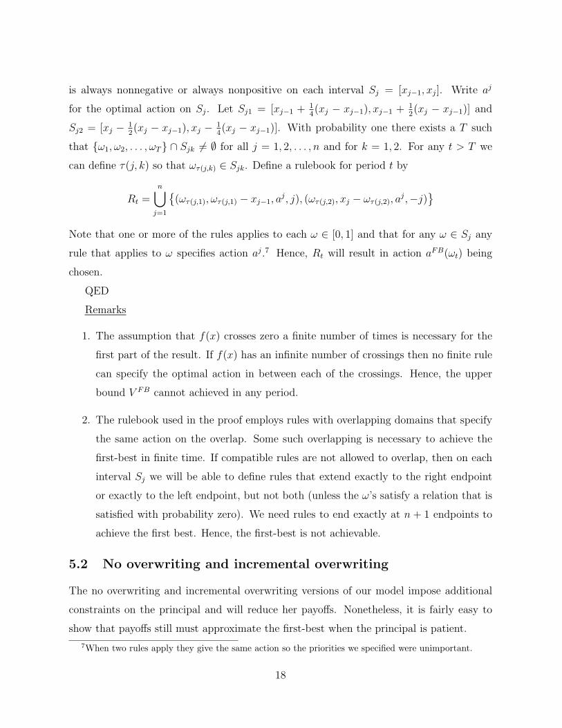
is always nonnegative or always nonpositive on each interval Sj = [xj−1, xj]. Write aj

for the optimal action on Sj. Let Sj1 = [xj−1 + 14(xj − xj−1), xj−1 + 1

2(xj − xj−1)] and

Sj2 = [xj − 12(xj − xj−1), xj − 1

4(xj − xj−1)]. With probability one there exists a T such

that ω1, ω2, . . . , ωT ∩ Sjk 6= ∅ for all j = 1, 2, . . . , n and for k = 1, 2. For any t > T we

can define τ(j, k) so that ωτ(j,k) ∈ Sjk. Define a rulebook for period t by

Rt =n⋃

j=1

(ωτ(j,1), ωτ(j,1) − xj−1, a

j, j), (ωτ(j,2), xj − ωτ(j,2), aj,−j)

Note that one or more of the rules applies to each ω ∈ [0, 1] and that for any ω ∈ Sj any

rule that applies to ω specifies action aj.7 Hence, Rt will result in action aFB(ωt) being

chosen.

QED

Remarks

1. The assumption that f(x) crosses zero a finite number of times is necessary for the

first part of the result. If f(x) has an infinite number of crossings then no finite rule

can specify the optimal action in between each of the crossings. Hence, the upper

bound V FB cannot achieved in any period.

2. The rulebook used in the proof employs rules with overlapping domains that specify

the same action on the overlap. Some such overlapping is necessary to achieve the

first-best in finite time. If compatible rules are not allowed to overlap, then on each

interval Sj we will be able to define rules that extend exactly to the right endpoint

or exactly to the left endpoint, but not both (unless the ω’s satisfy a relation that is

satisfied with probability zero). We need rules to end exactly at n + 1 endpoints to

achieve the first best. Hence, the first-best is not achievable.

5.2 No overwriting and incremental overwriting

The no overwriting and incremental overwriting versions of our model impose additional

constraints on the principal and will reduce her payoffs. Nonetheless, it is fairly easy to

show that payoffs still must approximate the first-best when the principal is patient.

7When two rules apply they give the same action so the priorities we specified were unimportant.

18

Proposition 6 Suppose that f(x) crosses zero a finite number of times. In the no overwrit-

ing and incremental overwriting models the principal’s average per-period payoff converges

to V FB in the limit as δ → 1.

Proof

A suboptimal strategy for the principal which is feasible in the incremental overwriting

model would be define no rule except in the 2n periods in which the current state falls into

one of the subintervals Sjk defined in the proof of Proposition 5 for the first time, and in

those to define the rule exactly as we do in that proof. If the principal follows this strategy

she will achieve a payoff V FB in all periods from some period T on. Hence, her average

payoff will be something that approaches V FB as δ → 1. Her optimal strategy yields a

higher payoff, and hence must also approach V FB.

The above strategy is not feasible in the no overwriting model because the principal

is restricted from issuing overlapping rules even when they disagree. More complicated

strategies can be used, however, to obtain a payoff that approximates the first best. One

way to do this is to define no rule unless the state is within ε of the center of one of the

Sj. There may be a long wait until such states occur, but once they have occurred in each

Sj the expected payoff in all future periods is at least 1− 2nε. This similarly puts a lower

bound on the payoff that a rational player can receive.

QEDRemark

1. The assumption that f(x) has a finite number of crossings is convenient for this

proof, but is not necessary. If f(x) crosses zero a countable number of times, we can

implement a similar strategy in each subinterval. Not all subintervals will be covered,

but each half of a subinterval of width w is covered with probability (1 − w2)t−1 in

period t. Hence, the expected payoff again converges to the first best.

A final result of this section is that when no overwriting is allowed the first-best is not

achieved in finite time.

Proposition 7 Consider the no overwriting version of our model and suppose that f has

a finite number of zeroes. Then at any finite time t E[πt] < πFB with probability one.

19

Proof The proof is by induction. At t = 0, D(R) = ∅. If at any time t > 0, D(R)\[0, 1]

is non-empty then there must exist a subinterval of [0, 1] with positive measure, [a, b] say,

which is not covered by a rule. Let ωt be the state at time t. By no overwriting a new rule

can only be created if ωt ∈ [a, b]. But if ωt 6= (a − b)/2 then the rule cannot cover [a,b],

and pr(ωt = (a− b)/2) = 0. Thus the induction is complete.

QED

6 Delegation Structures

So far our environment has been sufficiently simple that there has been a single possible

delegation structure for the authority relationship/firm: a single principal, a single agent

and a single task. We now consider a richer environment where the principal has a single

unit of time, but may do two things: perform a task herself, or communicate about it to

an agent. We assume that performing a task is more time consuming than communicating

about it. In particular, we assume that performing a task takes one unit of time, but

communicating to an agent takes only 1/2 a unit of time. The principal has two agents

available.

More concretely, there are two tasks i = 1, 2. On each task the principal’s payoff on

task i is πi(ai, ωi) that depends on the action taken and the state of nature. Suppose that

the principal’s benefit function for the two tasks is given by B(π1(a1, ω1), π2(a2, ω2)) =

min(π1(a1, ω1), π2(a2, ω2)) + (1 − γ)max(π1(a1, ω1), π2(a2, ω2)) and the “f functions” are

f1 and f2 respectively. Note that γ parameterizes the degree of complementarity of

the tasks, with γ = 1 being strict complementarity. As before, the principal’s pay-

off in the full game is the discounted sum of his per period payoffs and is given by

V =∑T

t=1 δtB(π1(a1, ω1), π2(a2, ω2)). There are three possible delegation structures in this

setting: (i) the principal communicates with each agent after observing ωt and then task

1 is performed by agent 1 and task 2 by agent 2 in period t + 1, (ii) task 1 is performed

by an agent and task 2 is performed by the principal, but without communication from

the principal, and (iii) task 2 is performed by an agent and task 1 is performed by the

principal, but without communication from the principal. We call these full delegation,

20

type 1 delegation and type 2 delegation respectively.

We can now offer a number of results about the relative attractiveness of different

delegation structures.

Proposition 8 Consider any of the overwriting assumptions, suppose that f(x) crosses

zero a finite number of times, and that delegation strategies are time invariant. Then if δ

is sufficiently large then full delegation is optimal.

Proof

From Propositions 5 and 6 we know that as δ → 1 the principal’s average per-period

payoff converges to V FB. Neither type 1 or type 2 delegation can achieve this since there is

no communication on one of the tasks and the expected payoff on that task is zero which

is bounded away from V FB, and the payoff on the other task is V FB.

QED

The next result shows that if the principal starts out with full delegation then he will

switch to type 1 or type 2 delegation if he gets enough “lucky” realizations of the state

which allow him to establish very effective rules on one task.

Proposition 9 Consider the vast overwriting version of the model and suppose that f(x)

crosses zero a finite number of times. Then with probability one there exists a T such that

type i delegation is optimal in all future periods t > T .

Proof

From Proposition 5 we know that with probability one there exists a T such that for

all t ≥ T , aFB(ωt) is chosen. If this happens on task 1 (respectively task 2) then type 1

delegation (respectively type 2 delegation) is optimal since aFB(ωt) is chosen on both tasks.

QED

Remarks

1. The proposition says that type i delegation is weakly optimal, but it will be strictly

optimal except in the special case where the first-best rulebook is established on both

tasks in exactly the same period.

21

2. It seems intuitive that if a highly effective rulebook is developed on one task relative

to that on the other task then it would be optimal for the principal to delegate the

task with the effective rulebook and perform the other himself. However, it is unclear

to us how to formalize this intuition at present.

While Proposition 8 showed that full delegation can be optimal if the principal is suffi-

ciently patient, we now show that if she is sufficiently impatient but the tasks are strongly

complementary then full delegation is optimal for some amount of time.

Proposition 10 Consider any of the overwriting regimes. Then if δ is sufficiently small

and γ is sufficiently close to one then there exists T ≥ 1 such that full delegation is optimal

for all t = 1, ..., T

Proof

At t = 1 the expected payoff from under full delegation is zero and no other governance

structure improves on this since the expected payoff on the delegated task is zero and γ is

close to 1 by assumption. At t = 2 the expected payoff at t = 1 on each task under full

delegation is positive, but under the other governance structures one task still has expected

t = 2 payoff of zero. Therefore for γ sufficiently close to 1 full delegation is optimal.

QED

A final observation of this section is that the path dependence which the basic model

exhibited can be magnified in this richer setting. There there was simply a direct effect of

history on payoffs. Here there is an additional indirect effect whereby a change in delegation

structure can further improve the principal’s payoff if he is able to switch to a more effective

delegation structure.

7 Endogenous Categories

As we mentioned in the introduction, our model suggests a mechanism via which categories

are formed in models of category based thinking (such as Mullainathan (2002) or Fryer and

Jackson (2007)). Roughly speaking, these models depart from the Bayesian framework by

22

grouping together multiple states into a single category. In Fryer and Jackson the decision

maker allocates experiences to a finite and limited number of categories–and they focus

on the optimal way to categorize (given the number categories available). They show that

experiences which occur less frequently are (optimally) placed in categories which are more

heterogeneous. Mullainathan (2002) considers decision makers who have coarser beliefs

than pure Bayesians, since they have a set of categories which are a partition of the space

of posteriors and choose just one category given data which they observe. They then

forecast using the probability distribution for the category.

An important question which these models leave open is where exactly these categories

come from. In Mullainathan (2002) they are completely exogenous. In Fryer and Jackson

(2007) they are formed optimally, although the number of categories is exogenous. Our

model provides one way to think about how categories are formed. In our setting we think

of the categories as being the sets ωs.t.‖ ω − ωt‖ < dt on which individual rules are

defined. Thus in an N period model if action 1 is taken on several disjoint set we think of

them as being different categories8. The analog of perfect categorization is that all states

are covered by a rule (with highest precedence) which maximizes the principal’s payoff.

Imperfect categorization comes from one of two sources: (i) rules which do not maximize

the principal’s payoff in a given state or, (ii) states which are not covered by a rule.

Fryer and Jackson (2007) offer a labor market example with high and low ability work-

ers who may be black or white. Thus there are for types: high-black, low-black, high-

white, low-white. They assume that the respective population shares of the types are:

5%, 5%, 45%, 45%. In the context of their model they show that if there are only three

categories then high and low ability blacks are categorized together, whereas high-white

and low-white each have their own category.

In the context of our model, suppose that action 1 is the decision to hire a worker and

action -1 is the decision not to hire. The left panel of figure 4 depicts an arrangement of

workers which (from left to right) is: high-white, low-white, low-black, high-black. The

dotted vertical line represents the division between whites and blacks. Now suppose that

there are two periods and the first period realization of the state is ω1. The optimal rule

8In the case of overlap a state can belong to multiple categories.

23

categorizes all workers in the band between the first and third dots together and the rule

is that any worker in that category should be hired. In a sense this rule is quite “fair”,

though not perfectly so. Most high ability blacks are categorized as to-be-hired, though

not all, and a few low ability whites are also put in that category.

-

6

?

HHHHH

HHHHHH

HHHH

ω1

r rr

ω

f(ω)

-

6

?

@@

@@

@

@@

@@

@EEEEEE

ω1rr r

ω

f(ω)

Figure 4: Categorization examples

In the second panel of figure 4 outcomes can be much less fair. The difference between

the two panels is the frequency of the function. This captures the idea that high and low

ability types are harder to distinguish than they are in the left panel–they are less naturally

clumped together. Not only can this lead to a less effective rule being developed, it can

lead to a less fair one. If the realization of the state is ω1 then the optimal rule categorizes

all workers between the first and third dots as not-to-be-hired. More than half the high-

ability blacks are so categorized, and this comes from the principal’s desire to expand the

rule on the left of ω1 so as to prevent many low-whites from being hired. The key driver

of the unfairness is that whites are relatively more populous than blacks. This is a similar

underlying cause as in Fryer and Jackson, though the models are obviously different. In a

version of our model with more than two periods both the number of categories and the

nature of the categorization arise endogenously.

24

8 Discussion and Conclusion

The model we have analyzed sheds light on a number of phenomena. The first is path

dependence, whereby there may be differences in performance based purely on the history

of events. In the model, a series of “lucky” early realizations of the state can lead to a very

effective rule book being established, delivering highly efficient outcomes. Conversely, bad

draws early on can have persistent effects which cannot be overcome. There is a sizeable

empirical literature which documents what Gibbons (2006) calls “persistent performance

differences among seemingly similar organizations”: that is, substantial differences in the

performance of organizations which are difficult to account for (Mairesse and Griliches

(1990), McGahan (1999), Chew et al. (1990)).

One potential theoretical explanation for this is that differences in performance corre-

spond to different equilibria of a repeated game (Leibenstein (1987)). As Gibbons (2006)

points out, such an explanation provides a basis for the existence of different equilibria,

but is silent about the dynamic path of differences, and how one might switch equilibria.

In contrast, our model exhibits path dependence. It can be the case that a firm has more

efficient communication than another purely because of chance: they got some good draws

early on which allowed them to develop and effective rule book.

Furthermore, the model with multiple activities highlights that there can be a compli-

cated evolution of governance structures because of communication needs. Various activ-

ities may or may not be delegated, and this can change over time as more effective rules

are developed. At a minimum this suggests that bounded communication is a potential

explanation for the heterogeneity of observed organizational forms.

The model also provides a potential explanation for learning curves, whereby a firm’s

cost declines with cumulative output/experience. The fact that learning can take place at

different rates depending on history or different abilities to overwrite is consistent with the

evidence on heterogeneity of rates of learning (Argote and Epple (1990)).

Another empirical regularity which has been documented is that firms often “start-

small” in the sense that they grow less quickly than they otherwise would. On its face this is

puzzling, as profits are being foregone in the process. Watson (2002) argues that a rationale

25

for starting small is to build cooperation in a low stakes environment and then enjoy the

benefits of the cooperative equilibrium in a high stakes environment. Our model offers a

different (and potentially complementary) notion of starting small. There is option value in

developing rules and consequently rules can be under-inclusive, particularly early on (recall

Proposition 2). One way to interpret the actions in our model that would make it connect

with the starting-small idea would be to regard the zero expected payoff that obtains in

states for which no rule has been defined as coming from a blanket instruction that the

firm should decline to decline any business opportunities that might arise which do not fall

into any of the categories for which rules have been defined. With this interpretation, our

model would be one in which the size of the business grows over time as new situations arise

and enable the firm to promulgate rules about how it should exploit such opportunities.

The possibility that communication may start out vague and become more precise over

time has the flavor of what Gibbons (2006) refers to as “building a routine”. The model

also highlights that the nature and extent of inefficiency from bounded communication–

and the degree to which rules are over or under inclusive–can depend importantly on the

ability of the principal to amend previously developed rules. Indeed we saw that in the vast

overwriting regime there was no option value from leaving rules undefined as they could

always be amended.

There are two obvious directions for further work. The first is to provide a more concrete

foundation for the inability of the principal to describe the state to the agent. We remarked

early on that we had in mind state spaces which were complex in some sense, though we

conducted our analysis on the unit interval. It would be useful to understand what kinds

of environments, or what other cognitive limitations, give rise to the inability to perfectly

communicate.

Finally, the second direction would be to more explicitly model the tradeoff between

the price mechanism and the authority relationship. This would allow one to address the

question of when the price mechanism is superior at adapting to changing circumstances

than the authority relationship: Barnard versus Hayek. What we have done is to highlight

one particular cost of the authority relationship, and analyzed how different governance

structures perform in that context. We remarked earlier that a complete understanding of

26

the tradeoff between the efficiency of markets and firms in changing circumstances would

seem to require a general model of price formation. That is, a model in which one can

analyze how frictions affect the incorporation of information into the price mechanism and

hence the circumstances in which the price mechanism works well and those where it does

not. Although the literature on rational expectations equilibrium and securities markets

provided some steps in this direction9, we are not aware of a suitable model for studying this

question. For that model would not only need to address the question of how information

is incorporated into prices, but also be able to rank economies according to the allocative

efficiency effects of imperfect prices. Even the first question is daunting enough. Any model

of price formation with rational expectations is subject to the Milgrom-Stokey No-Trade

Theorem (Milgrom and Stokey (1982)), raising the awkward question of how information

comes to be incorporated into prices if those who collect the information cannot benefit

from it. Nonetheless, a complete model of price formation seems essential to satisfactorily

answer the larger question of when markets or firms adapt better to changing circumstances.

9For example: Grossman (1976), Allen (1981), Glosten and Milgrom (1985), Kyle (1985)

27

References

Beth Allen. Generic existence of completely revealing equilibria for economies with uncer-

tainty when prices convey information. Econometrica, 49:1173–1199, 1981.

Linda Argote and Dennis Epple. Learning curves in manufacturing. Science, 247:920–924,

1990.

Kenneth J. Arrow. The Limits of Organization. Norton, New York, NY, 1974.

Kenneth J. Arrow. On the agenda of organizations. In Collected Papers of Kenneth J.

Arrow, volume 4, chapter 13, pages 167–184. Belknap Press, 1984.

George Baker, Robert Gibbons, and Kevin J. Murphy. Governing adaptation: Decision

rights, payoff rights, and relationships in firms, contracts, and other governance struc-

tures. Mimeo, 2006.

Chester Barnard. The Functions of the Executive. Harvard University Press, Cambridge,

MA, 1938.

Bruce Chew, Kim Clark, and Timothy Bresnahan. Measurement, coordination and learning

in a multiplant network, chapter 5. Harvard Business School Press, 1990.

Ronald Coase. The nature of the firm. Economica, 4:396–405, 1937.

Jacques Cremer, Luis Garicano, and Andrea Prat. Language and the theory of the firm.

Quarterly Journal of Economics, CXXII:373–408, 2007.

Roland G. Fryer and Matthew O. Jackson. A categorical model of cognition and biased

decision-making. Contributions in Theoretical Economics, B.E. Press, fortchoming, 2007.

Robert Gibbons. What the folk theorem doesn’t tell us. Industrial and Corporate Change,

15:381–386, 2006.

Lawrence R. Glosten and Paul R. Milgrom. Bid, ask and transactions prices in a specialist

model with heterogenously informed traders. Journal of Financial Economics, 14:71–100,

1985.

28

Sanford Grossman and Oliver Hart. The costs and benefits of ownership: A theory of

vertical and lateral ownership. Journal of Political Economy, 94:691–719, 1986.

Sanford J Grossman. On the efficiency of competitive stock markets where traders have

diverse information. Journal of Finance, pages 573–585, 1976.

Oliver Hart and John Moore. Property rights and the nature of the firm. Journal of

Political Economy, 98:1119–1158, 1990.

F.A. Hayek. The use of knowledge in society. American Economic Review, 35:519–530,

1945.

Benjamin Klein, Robert Crawford, and Armen Alchian. Vertical integration, appropriable

rents and the competitive contracting process. Journal of Law and Economics, 21:297–

326, 1978.

Frank H. Knight. Risk, Uncertainty, and Profit. Hart, Schaffner & Marx; Houghton Mifflin,

Boston, MA, 1921.

Albert S. Kyle. Continuous auctions and insider trading. Econometrica, 53:1315–1335,

1985.

Harvey Leibenstein. Inside the Firm: The Inefficiencies of Hierarchy. Harvard University

Press, 1987.

Jacques Mairesse and Zvi Griliches. Heterogeneity in panel data: are there stable produc-

tion functions. In P. Champsaur et al., editor, Essays in Honor of Edmond Malinvaud,

volume 3: Empirical Economics. MIT Press, Cambridge MA, 1990.

Jacob Marschak and Roy Radner. Economic Theory of Teams. Cowles Foundation and

Yale University, 1972.

Anita M. McGahan. The performance of us corporations: 1981-1994. Journal of Industrial

Economics, XLVII:373–398, 1999.

29

Paul Milgrom and Nancy Stokey. Information, trade and common knowledge. Journal of

Economic Theory, 26:17–27, 1982.

Sendhil Mullainathan. Thinking through categories. NBER working paper, 2002.

Sendhil Mullainathan, Joshua Schwartzstein, and Andrei Shleifer. Coarse thinking and

persuasion. Quarterly Journal of Economics, forthcoming, 2008.

Herbert Simon. A formal theory model of the employment relationship. Econometrica, 19:

293–305, 1951.

Joel Watson. Starting small and commitment. Games and Economic Behavior, 38:176–199,

2002.

Oliver Williamson. Transaction cost economics: The governance of contractual relation-

ships. Journal of Law and Economics, 22:233–261, 1979.

Oliver E. Williamson. The vertical integration of production: Market failure considerations.

American Economic Review, 61:112–123, 1971.

Oliver E. Williamson. The economics of governance. American Economic Review Papers

and Proceedings, 2:1–18, 2005.

30