
A Theory of Retirement - The National Bureau of Economic ...A Theory of Retirement David E ... We...
41
NBER WORKING PAPER SERIES A THEORY OF RETIREMENT David E. Bloom David Canning Michael Moore Working Paper 13630 http://www.nber.org/papers/w13630 NATIONAL BUREAU OF ECONOMIC RESEARCH 1050 Massachusetts Avenue Cambridge, MA 02138 November 2007 Research for this article was funded by NIH grant # 5 P30 AG024409-04. The views expressed herein are those of the author(s) and do not necessarily reflect the views of the National Bureau of Economic Research. © 2007 by David E. Bloom, David Canning, and Michael Moore. All rights reserved. Short sections of text, not to exceed two paragraphs, may be quoted without explicit permission provided that full credit, including © notice, is given to the source.
Transcript of A Theory of Retirement - The National Bureau of Economic ...A Theory of Retirement David E ... We...

NBER WORKING PAPER SERIES
A THEORY OF RETIREMENT
David E. BloomDavid CanningMichael Moore
Working Paper 13630http://www.nber.org/papers/w13630
NATIONAL BUREAU OF ECONOMIC RESEARCH1050 Massachusetts Avenue
Cambridge, MA 02138November 2007
Research for this article was funded by NIH grant # 5 P30 AG024409-04. The views expressed hereinare those of the author(s) and do not necessarily reflect the views of the National Bureau of EconomicResearch.
© 2007 by David E. Bloom, David Canning, and Michael Moore. All rights reserved. Short sectionsof text, not to exceed two paragraphs, may be quoted without explicit permission provided that fullcredit, including © notice, is given to the source.

A Theory of RetirementDavid E. Bloom, David Canning, and Michael MooreNBER Working Paper No. 13630November 2007JEL No. D91,J26
ABSTRACT
We construct a life-cycle model in which retirement occurs at the end of life as a result of declininghealth. We show that improvements in life expectancy, coupled with a delay in the onset of disability,increases both the optimal consumption level and the proportion of life spent in leisure. The retirementage increases proportionally less than the increase in life expectancy.
David E. BloomHarvard School of Public HealthDepartment of Population and International Health665 Huntington Ave.Boston, MA 02115and [email protected]
David CanningHarvard School of Public HealthDepartment of Population and International Health665 Huntington Ave.Boston, MA [email protected]
Michael MooreQueen's University BelfastRoom 26.G0125 University SquareBelfast, BT7 1NN [email protected]

1
1. Introduction
Improvements in life expectancy and living standards over the last 150 years reflect a dramatic
increase in human welfare. For the world as a whole, life expectancy at birth rose from around
30 years in 1900 to 65 years by 2000 (and is projected to rise to 81 by the end of this century;
Lee 2003). These improvements have not only resulted in a large direct gain in welfare
(Nordhaus 2003, Becker, Philipson, and Soares 2005) but have also had a profound influence on
life-cycle behavior through changes in the time horizons of individuals (Hamermesh 1985).
In this paper we extend the Blanchard-Yaari-Weil model of consumption with finite lives
and perfect annuity markets to endogenously determine both retirement and the time path of
consumption. We use the model to show how optimal retirement and savings decisions respond
to changes in wage levels and life expectancy. Standard concavity conditions usually imply the
smoothing of leisure over time. The lumping of leisure at the end of life requires some force that
deters working when old. We explain retirement as the result of rising ill health with age, which
increases the disutility of labor and reduces the productivity of working.
Although health declines with age, rising life spans have been accompanied by improving
age-specific health status; that is, our lives are both longer and healthier. The ‘compression of
morbidity’ hypothesis (Fries 1980), maintains that the average age at first infirmity, disability, or
other morbidity is postponed to such an extent that the period of ill health at the end of life is
compressed. Increases in life expectancy in the United States over the last two centuries have
indeed been associated with reductions in the age-specific incidence of disease, disability, and
morbidity (Costa 2002; Fogel 1994, 1997). This trend is continuing (Crimmins, Saito, and
Ingegneri 1997; Freedman, Martin and Schoeni 2002). We model the compression of morbidity

2
by assuming that the age of onset of disability rises proportionately, or more than
proportionately, with life expectancy.
We examine the optimal choices of agents in a model with complete markets. An
increase in life span has an "income" effect in that it enlarges the budget set. It also generates
substitution effects by changing the rewards to working and saving. Our model shows that,
under standard assumptions on preferences, the income effect tends to dominate, producing both
increased consumption and leisure when life expectancy increases. Indeed the wealth effect of
an increase in life expectancy will reduce the proportion of life span devoted to work, though it is
unlikely to reduce the absolute length of the working life. The level of wages also has income
and substitution effects. In our model increases in the level of wages will reduce the length of the
working life if the worker’s inter-temporal elasticity of substitution with respect to consumption
is less than one (corresponding to a coefficient of relative risk aversion greater than one).
We use these results to argue that the long-term decline in the age of retirement in
industrial countries over the last 150 years (i.e., that the labor force participation rate of men in
the United States aged 65 and older declined from around 80 percent in 1850 to less than 20
percent by 2000 (Costa 1998b)) has been due to the increasing level of wages, which coincides
with Costa’s (1998a) analysis.
In addition to offering a positive theory for observed behavior, our approach offers a
method through which to estimate the welfare effects of proposed changes to social security
systems. Assuming that social security systems desire to promote the optimal retirement and
consumption outcomes rational agents would make with complete markets, the results of our
model can serve as a benchmark in the design of public pension systems.

3
A natural approach to dealing with solvency problems that arise in a social security
system when life expectancy increases is to increase contribution rates and to reduce benefit
rates. By contrast, our model implies that the optimal response should be to reduce contribution
rates and increase benefit rates, maintaining solvency exclusively by increasing the age of
retirement, though this age can rise less than proportionately with life expectancy. This response
can maintain solvency because rising wages over time and compound interest on accumulated
savings mean that longer working lives tend to create more than proportionately higher wealth at
retirement. We show that under standard assumptions on interest rates and wage growth, and
given projected changes in age specific survival curves, such a plan is feasible.
Several papers have tackled the issue of how changes in longevity affect retirement and
consumption decisions. The approach most similar to ours is that of Chang (1991) who argues
that in competitive markets a rise in life expectancy reduces consumption and increases savings
rates. The major difference between Chang’s model and ours is his assumption that the forces
that give rise to retirement at each age (low wages and a high disutility of labor) remain
unchanged when life expectancy rises. By contrast, we assume that healthy life expectancy also
rises, making a longer working life more palatable. Chang (1991) and Kalemli-Ozcan and Weil
(2002) also emphasize that with no annuity markets a reduction in mortality rates increases the
effective return to saving and encourages saving and early retirement when life expectancy rises.
Here we emphasize that the wealth effect, which leads to increased consumption (reduced
saving) and more leisure, tends to dominate when markets are complete.
We present our model in section 2, and in section 3 we show how the dynamic
programming problem facing agents generates a set of equations (derived from the first-order
conditions) that determine the optimal retirement age and consumption profile. In section 4 we

4
use the model to investigate the effect of increases in healthy life span and wages on savings and
retirement behavior and present our results. Section 5 discusses the implications of our results
for social security systems and section 6 makes some concluding remarks.
2. The Model
This life-cycle theory of saving and retirement is not a complete model of saving and
retirement behavior. There are several influences that it does not incorporate. For example,
people may engage in precautionary saving to guard against income shocks, and they may also
save to provide bequests (Skinner 1985). In addition, whereas in many developing countries the
elderly are supported to a large extent by intra-family transfers, in many industrial countries the
elderly derive considerable support from social security systems. These transfer systems clearly
affect incentives to save and to retire. Notwithstanding its limitations, the life-cycle model can
provide valuable insights into behavior. In addition, optimal decisions by individuals with
complete markets generate an efficient outcome that can be used to guide policy even under
market imperfections.
Our formal life cycle model makes a number of simplifying assumptions. We assume
that the mortality schedule is exogenous, which ignores the possibility of using consumption and
health services to extend longevity (Ehrlich and Chuma 1990) or of a reverse link from labor
supply to health status and life expectancy. In the interest of simplicity, we also assume that the
life cycle has no period of schooling. Schooling will affect the productivity of workers, their
health and longevity, and their utility of leisure (Heckman 1976) complicating a retirement -
consumption model.

5
We begin with mortality. We assume that there is a family of possible survival schedules
indexed by a single variable λ . There is a survival schedule ( , )s t λ that gives the probability of
survival to age t. The mortality rate at time t is
( , )
( , ) -( , )
ds tdtm ts t
λλ
λ= (1)
and life expectancy is given by1
0 0
( ) ( , ) ( , ) ( , )T T
z t m t s t dt s t dtλ λ λ λ= =∫ ∫ (2)
We assume that there is a biological maximum, T , to the length of life (Carnes,
Olshansky, and Grahn, 2003). Let us assume that as the index λ increases, mortality at each age
falls, so that survival to each age rises, as does overall life expectancy, z, and that this
relationship is invertible. Lee and Miller (2001) show using empirical data that in practice the
Lee and Carter (1992) method of indexing mortality rates generates a monotonic relationship
between the index and the age-specific mortality rates; adopting this method of indexing would
therefore imply an invertible mapping between the parameter λ and life expectancy. Assuming a
one-to-one mapping from life expectancy to our index of mortality, we can take life expectancy
to be a unique identifying index for a mortality schedule. In what follows we therefore use life
expectancy at the beginning of working life, z, as our index of the mortality schedule and write
mortality2 as ( , )m t z .
1 The probability that your age of death is exactly t is the probability of surviving to t times the mortality rate at t. The second equality comes from substituting in for the mortality rate and integrating by parts using the fact that
(0, ) 1s λ = and ( , ) 0s T λ = . 2 Note that we do not impose the Lee-Carter functional form; we only specify that there is a one-to-one mapping from mortality schedules to life expectancy so that life expectancy identifies a mortality schedule.

6
A major innovative feature of our model is the health schedule ( , )h t z . We assume that
health declines with age t. In addition, we postulate that health at age t depends on life
expectancy, z. If health is independent of z, it implies that increases in life expectancy are not
associated with general health improvements in the form of reductions in morbidity (sickness),
which implies further that population aging is associated with an increasingly large share of
unhealthy people.
However, evidence points in the opposite direction. Not only are people living longer,
but age specific disability is also falling. Cutler (2001) attributes reductions in disability at older
ages to long-term protective effects of reduced disease exposure in childhood, rising levels of
education and socio-economic status, improved health-related behavior such as reductions in
smoking, improved medical care, and the use of special aids to reduce disability for a given
health state. Manton, Gu, and Lamb (2006) estimate that between 1935 and 1982 life expectancy
and (disability-free) active life expectancy at age 65 both moved up in the United States, keeping
the proportion of disability-free life after 65 relatively steady at around 73%. However, between
1982 and 1999 life expectancy at age 65 rose from 16.9 to 17.7 years while active life
expectancy rose from 12.3 to 13.9 years. This implies a rise in the proportion of disability-free
life to over 78%, and a reduction in the absolute time spent in disability from 4.6 to 3.8 years.
The compression of morbidity, either absolute or relative, appears to hold in most developed
countries (Mor 2005). Although time-series evidence in developing countries is scarce, Mathers
et al. (2001) show that across countries health-adjusted life expectancy (each life year weighted
by a measure of health status) increases as fast as total life expectancy, implying a rising
proportion of healthy to total life expectancy as life expectancy increases.

7
Although the compression of disability, at least in the recent past, in the United States
seems evident, and although disability is a cause of retirement (Gordo 2006), most people retire
before the onset of severe disability. Despite the fact that they may still be physically capable of
working, moderate ill health not amounting to disability may deter their participation in the labor
force. The “dynamic equilibrium” hypothesis suggests the compression of time spent in severe
disability may be the result of reducing the transition rate from low or moderate ill health to
severe disability. This in turn may result in an increase in the prevalence of less-severe disability
states (e.g., Graham et al. 2004).
To examine the effect of the compression of morbidity we begin by taking as our
benchmark the case where healthy life span increases proportionately with overall life span. We
assume that:
( , ) ( , ) 0h t z h t z forρ ρ ρ= > (3)
Note that we assume both age and life expectancy are measured from the start of adult
life. If a particular level of health is labeled “disabled,” equation (3) implies that the age of onset
of this “disabled” health rises proportionately with life expectancy. We examine this case below,
and discuss how our results extend to the case where healthy life spans increase faster than life
expectancy allowing for the absolute compression of morbidity.
We denote labor supply at time t by tχ , which is assumed to lie in the closed
interval[0,1] . Utility is assumed to be strongly separable in goods and leisure and is given by
( ( )) ( ) ( ( , ))u c t t v h t zχ− (4)
where ( )c t is consumption at age t and ( ( , ))v h t z is the disutility of working given the health
state ( , )h t z . We assume that u is twice differentiable with '( ) 0, "( ) 0u c u c> < and that the

8
disutility function v satisfies '( ) 0v h < so that the disutility of work (and the relative utility of
leisure) is higher when health is poorer. Lifetime expected utility is
[ ]0
( , ) ( ( )) ( ) ( ( , ))T
tU e s t z u c t t v h t z dtδ χ−= −∫ (5)
where δ is the subjective rate of time preference, and T is the biological maximum life span.
The wage earned by a worker with health h is given by
1 2( , ) ( ) ( ( , ))w t h w t w h t z= (6)
The term 1( )w t captures the change in wages over time due to exogenous forces, for example,
technical progress, and 2 ( ( , ))w h t z captures the fact that worker productivity depends on health,
which is a function of age relative to life expectancy. We assume 1( ) 0w t′ ≥ and 2 ( ) 0w h′ ≥ so that
wages are increasing over time due to exogenous forces and are increasing in health. The
multiplicative functional form implies that the health effect on log wages is additive, which is
consistent with a Mincer wage equation that includes health as a form of human capital as in
Schultz (1999). Chang (1991) and Kalemli-Ozcan and Weil (2002) have exogenous age-wage
schedules that do not change as life expectancy varies; we allow for an effect of life expectancy
on wages through improved health.
Wealth, W , evolves according to
( )1 2( ) ( ) ( ( , )) ( , ) ( ) ( )dW t w t w h t z m t z r W t c tdt
χ= + + − (7)
If the agent works at time t, he or she earns the wage 1 2( ) ( ( , ))w t w h t z , and this is added to wealth.
Consumption, ( )c t , reduces wealth, while the stock of wealth earns a return, ( , )m t z r+ . We
assume that health may affect labor productivity and wages. We assume that wealth can be
transferred from one period to another by saving or borrowing from the financial sector. This

9
competitive financial sector can borrow or lend freely at the interest rate r. Agents are paid an
effective interest rate ( , )m t z r+ on their savings, which is larger than r, to compensate them for
the fact that they may die before withdrawing their savings. Similarly, agents who borrow pay
the rate ( , )m t z r+ to compensate the bank for the fact that they may die before repaying their
borrowings. This is equivalent to treating all savings as being in the form of annuity purchases,
while assuming that all borrowing has to be accompanied by an actuarially fair life insurance
contract for the amount of the loan.
Provided that a continuum of agents exists, the financial sector can avoid all risk by
aggregating over individuals thereby earning zero profits. The transfer of wealth from those who
die to the financial sector exactly compensates deposit-taking institutions for the fact that they
pay an interest rate ( , )m t z r+ on deposits that exceed the risk-free rate r, and rules out the need
to consider unintended bequests. The budget constraint is:
1 20 0
( , ) ( ) ( , ) ( ) ( ) ( ( , ))T T
rt rte s t z c t dt e s t z t w t w h t z dtχ− −≤∫ ∫ (8)
The control variables for the agent's optimization problem are and c χ . Agents must decide
when to work and what their consumption stream should be.3
We assume the boundary conditions:
1 2
1 2
(0) ( (0, )) '(0) ( (0, ))( ) ( ( , )) '(0) ( ( , ))
w w h z u v h zw T w h T z u v h T z
><
(9)
The first boundary condition implies that the disutility of working at age zero is sufficiently low
to ensure that the agent always prefers to work at the start of life, rather than live with no
consumption. The second boundary condition implies that the disutility of working at the
maximum possible age is sufficiently high that the agent always prefers to be retired. 3 Adding the direct utility of health as an additive term to the utility function does not affect decision making in any way.

10
It what follows we will assume that the rate of interest, r , is positive and equals the rate
of time preference, δ . Our theory is developed for the case where the growth rate of the
exogenous component of wages is moderate. If wage growth is very rapid a retired worker may
renter the labor market to take advantage of the high wages when old. To rule this out we
assume that for every life expectancy, the rate of growth of the disutility of labor with age
exceeds the exogenous component in the rate of growth of wages at each point in time:
1
1
w vw v
<& &
(10)
We show that this condition will imply that retirement occurs only once and is never reversed.
In this case we can label the retirement age as R .
3. Optimal Retirement and Consumption Decisions
The Hamiltonian for this problem is
[ ]
( )1 2
( , ) ( ( )) ( ) ( ( , ))
( )[ ( ) ( ) ( ( , )) ( , ) ( ) ( )]
tH e s t z u c t t v h t z
t t w t w h t z m t z r W t c t
δ χ
φ χ
−= −
+ + + − (11)
The first-order conditions for a maximum in and c χ are:
( )( ( , ))H t r m t zW
φ φ∂= − = − +
∂& , (12)
( )( , ) ( ) ( ) 0tH e s t z u c t tc
δ φ−∂ ′= − =∂
, and (13)
1 2
1 2
1 2
( , ) ( ( , )) ( ) ( ) ( ( , )) 0 when ( ) 1
( , ) ( ( , )) ( ) ( ) ( ( , )) 0 when ( ) (0,1)
( , ) ( ( , )) ( ) ( ) ( ( , )) 0 when ( ) 0
t
t
t
H e s t z v h t z t w t w h t z t
H e s t z v h t z t w t w h t z t
H e s t z v h t z t w t w h t z t
δ
δ
δ
φ χχ
φ χχ
φ χχ
−
−
−
∂= − + ≥ =
∂∂
= − + = ∈∂∂
= − + ≤ =∂
(14)
11
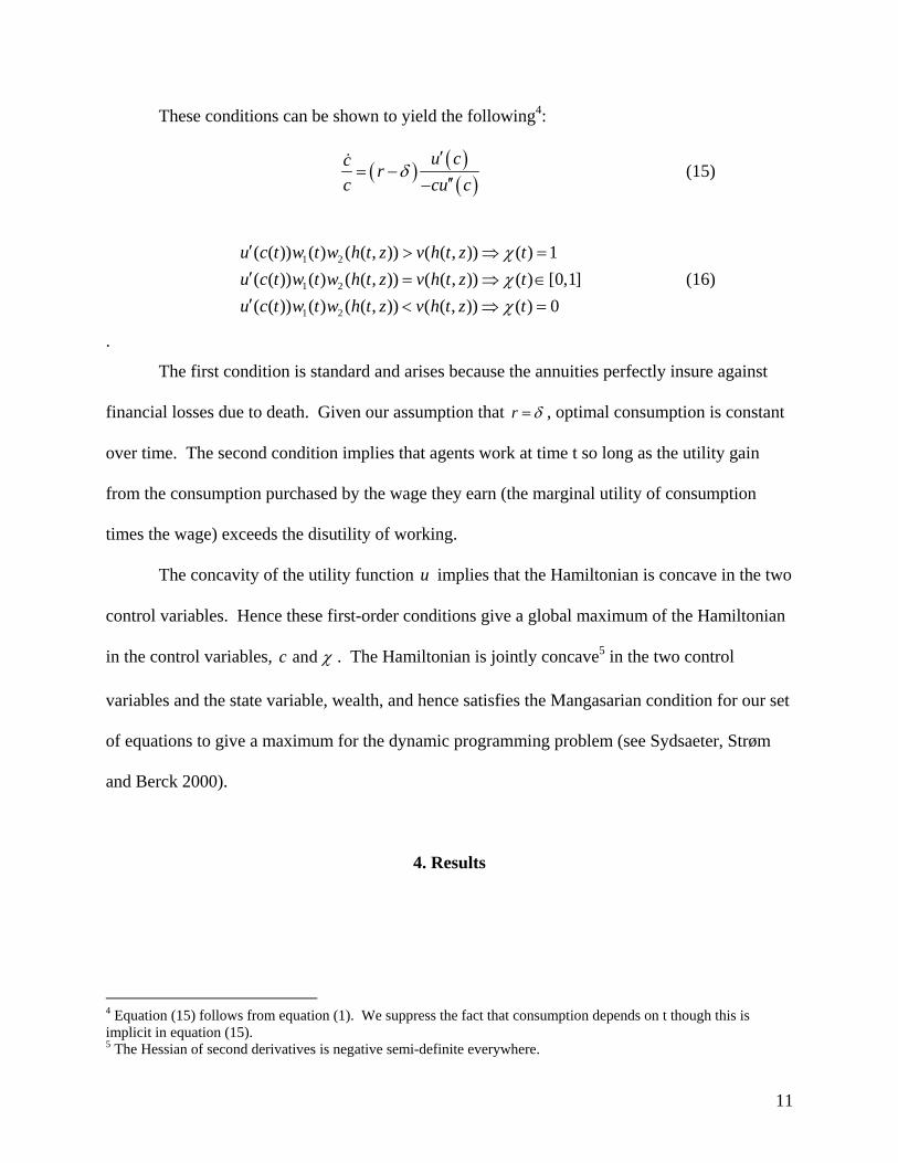
These conditions can be shown to yield the following4:
( ) ( )( )
u cc rc cu c
δ′
= −′′−
& (15)
1 2
1 2
1 2
( ( )) ( ) ( ( , )) ( ( , )) ( ) 1( ( )) ( ) ( ( , )) ( ( , )) ( ) [0,1]( ( )) ( ) ( ( , )) ( ( , )) ( ) 0
u c t w t w h t z v h t z tu c t w t w h t z v h t z tu c t w t w h t z v h t z t
χχχ
′ > ⇒ =′ = ⇒ ∈′ < ⇒ =
(16)
.
The first condition is standard and arises because the annuities perfectly insure against
financial losses due to death. Given our assumption that r δ= , optimal consumption is constant
over time. The second condition implies that agents work at time t so long as the utility gain
from the consumption purchased by the wage they earn (the marginal utility of consumption
times the wage) exceeds the disutility of working.
The concavity of the utility function u implies that the Hamiltonian is concave in the two
control variables. Hence these first-order conditions give a global maximum of the Hamiltonian
in the control variables, and c χ . The Hamiltonian is jointly concave5 in the two control
variables and the state variable, wealth, and hence satisfies the Mangasarian condition for our set
of equations to give a maximum for the dynamic programming problem (see Sydsaeter, Strøm
and Berck 2000).
4. Results
4 Equation (15) follows from equation (1). We suppress the fact that consumption depends on t though this is implicit in equation (15). 5 The Hessian of second derivatives is negative semi-definite everywhere.

12
Proposition 1 (a) It is optimal for an agent to begin life working, retire at age R, and not to work
thereafter. (b) The retirement age and consumption stream that maximize expected lifetime
utility are unique.
Proof: see appendix 1.
We first prove that any optimal plan has a single and irreversible retirement age. We then
prove that this optimal plan is unique. Note that retirement emerges endogenously from our
model. In our framework a lack of health effects on the disutility of labor and wages, combined
with exogenous wage growth, would tend to produce leisure in youth when wages are low, and
work when old and wages are high; the health effects are essential for our model to produce
retirement.
At the beginning of life the disutility of labor is low and the benefits of working in terms
of additional consumption spread over the life cycle are large. As life proceeds, rising disability
eventually outweighs the benefits of working, and retirement occurs.
Given proposition 1 we can rewrite the budget constraint as:
1 20 0
( , ) ( ) ( , ) ( ) ( ( , ))T R
rt rte s t z c t dt e s t z w t w h t z dt− −≤∫ ∫ (17)
In what follows we think of the choice variables as the consumption level and the
retirement age, with these chosen subject to equation (17). Consumption is steady over the life
cycle. Rising wages for young workers can lead to dis-saving when young before saving in
middle age in preparation for retirement when old, as occurs in the examples shown in appendix
1.

13
Consider what happens if life expectancy increases. Lee and Goldstein (2003) argue that
a natural benchmark for responding to an increase in life expectancy is to adjust the timing of all
life course choices proportionately. Bloom, Canning, and Graham (2003) show that in the case
of a certain life span, the optimal response to an increase in life span and health is to increase
working life proportionately keeping consumption unchanged, provided that interest rates, time
preference rates, and exogenous wage growth are all zero. In our framework, however, it is not
clear that such a proportional response is even feasible. Consider an initial life expectancy
0z and let the optimal retirement age be *0R and the optimal consumption level be *
0c . Let the
optimal retirement age at the longer life expectancy, 1z , be *1R and the optimal consumption
level be *1c . We require that the old consumption stream is affordable at the new survival
schedule provided retirement is postponed in line with life expectancy.6 We call this the
proportionality condition:
*0 1 0/
*1 0 1 1 2 1 1 0
0 0
( , ) ( , ) ( ) ( ( , ))R z zT
rt rte s t z c dt e s t z w t w h t z dt for z z− −≤ >∫ ∫ (18)
This proportionality condition may not be satisfied if the extension in life expectancy is
due to a rise in the survival schedule concentrated in the period immediately after retirement.
However, if the gain in life span comes from a more general reduction in mortality rates that
generates survival increases during the working life (which add to labor income) or near the end
of life (where consumption is heavily discounted), the additional income generated by
proportionately later retirement will be sufficient to keep consumption unchanged.
In practice, this condition is satisfied in historical data and future projections for the
United States. In Appendix 2 we examine cohort survival schedules for the United States (the
6 Note that by proposition 1 we can summarize labor supply by a retirement age. We integrate labor income over time up to retirement to get the value of lifetime earnings.

14
survival curve faced by the cohort) for different birth years. Using long run averages for the real
interest rate and wage growth, we show that moving from the survival schedule of those born in
1900 to those born in 1925, 1950, 1975, or 2000 (based on historical cohort survival rates and
projected rates) with an increase in the retirement age proportional to the increase in life
expectancy, would in each case allow consumption to increase. This means that it has been
feasible to keep the working life proportional to life expectancy with consumption unchanged.
We begin by giving results for the relative compression of morbidity as set out in
equation (3). We will later extend this result to the case in which compression of morbidity is
more than proportional.
Proposition 2: If there is proportional compression of morbidity, and changes in the survival
schedule satisfy the proportionality condition, the optimal response to an increase in life
expectancy requires consumption to stay the same or increase.
Proof: see Appendix 3.
The intuition for this result is that it is possible for the agent to increase working life
proportionately but keep consumption unchanged. In general the agent will do better than this.
If both leisure and consumption are normal goods the agent will take some of the additional
welfare in the form of consumption and some in the form of increased leisure.
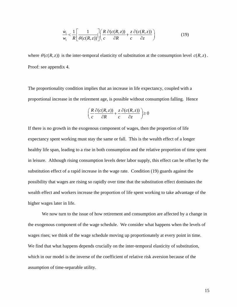
Proposition 3: If changes in the survival schedule satisfy the proportionality condition, the
optimal response to an increase in life expectancy requires the retirement age to rise less than
proportionately to life expectancy if and only if
15
1
1
1 1 ( ( , )) ( ( , ))( ( , ))
w R c R z z c R zw R c R z c R c zθ
⎡ ⎤ ∂ ∂⎛ ⎞< +⎜ ⎟⎢ ⎥ ∂ ∂⎝ ⎠⎣ ⎦
& (19)
where ( ( , ))c R zθ is the inter-temporal elasticity of substitution at the consumption level ( , )c R z .
Proof: see appendix 4.
The proportionality condition implies that an increase in life expectancy, coupled with a
proportional increase in the retirement age, is possible without consumption falling. Hence
( ( , )) ( ( , )) 0R c R z z c R zc R c z∂ ∂⎛ ⎞+ ≥⎜ ⎟∂ ∂⎝ ⎠
If there is no growth in the exogenous component of wages, then the proportion of life
expectancy spent working must stay the same or fall. This is the wealth effect of a longer
healthy life span, leading to a rise in both consumption and the relative proportion of time spent
in leisure. Although rising consumption levels deter labor supply, this effect can be offset by the
substitution effect of a rapid increase in the wage rate. Condition (19) guards against the
possibility that wages are rising so rapidly over time that the substitution effect dominates the
wealth effect and workers increase the proportion of life spent working to take advantage of the
higher wages later in life.
We now turn to the issue of how retirement and consumption are affected by a change in
the exogenous component of the wage schedule. We consider what happens when the levels of
wages rises; we think of the wage schedule moving up proportionately at every point in time.
We find that what happens depends crucially on the inter-temporal elasticity of substitution,
which in our model is the inverse of the coefficient of relative risk aversion because of the
assumption of time-separable utility.

16
Proposition 4: When the level of wages rises the optimal response of the agent is to
(i) keep retirement unchanged and increase consumption proportionally with wages if the utility
function has a local inter-temporal elasticity of substitution of unity.
(ii) increase the age of retirement and increase consumption more than proportionally with wages
if the utility function has a local inter-temporal elasticity of substitution greater than unity.
(iii) decrease the age of retirement and increase consumption less than proportionally with wages
if the utility function has a local inter-temporal elasticity of substitution less than unity.
Proof: see Appendix 5.
It is well known that the impact of wages on consumption and the demand for leisure has both
income and substitution effects. The pivotal case occurs where there is relative risk aversion that
is locally unity. We state this proposition to show that the result applies to our model. The long-
term decline in the retirement age, and increase in retirement savings, is consistent with an inter-
temporal elasticity of substitution less than unity (which in our model implies a coefficient of
relative risk aversion that exceeds one).
We now turn to the case where we have health improvements that are greater than
proportional to the rise in life expectancy:
( , ) ( , ) 1h t z h t z forρ ρ ρ> > (20)
This allows for age specific health status to rise more than proportionately with life expectancy
and is compatible with an absolute compression of morbidity. Proposition 1 clearly continues to
hold because it investigates the optimal retirement path for a fixed life expectancy. Similarly

17
proposition 4 reflects the effect of changing wage levels with a fixed life expectancy and so does
not depend on how health changes with life expectancy.
Proposition 2, which argues that consumption must rise when life expectancy and health
rise proportionately, continues to hold. Condition (3) is used at only one point in the proof in a
chain of inequalities and this chain continues to hold if we employ condition (20) instead. The
intuition is that with condition (20) the wealth effect gets larger, and wages at each age rise with
better health allowing higher consumption. Only proposition 4 changes if we adopt condition
(20) instead of condition (3). The higher wages and lifetime consumption will again promote
earlier retirement relative to life expectancy, but the better health at older ages increases
productivity and wages, while reducing the disutility of labour. These health effects, coupled
with rising exogenous wages, can create a substitution effect promoting work that may result in
working life rising faster than proportionately than life expectancy.
We focus on the effects of changes in life expectancy and the level of wages on
retirement and saving decisions. Bloom, Canning, and Moore (2004) also investigate the effects
of changes in the interest rate, rate of time preference, and the rate of wage growth under more
restrictive functional forms for utility and mortality.
5. Implications for Social Security
Our results give the optimal retirement and savings behavior of fully rational agents
under complete capital markets. In practice, imperfect capital markets (particularly annuity
markets), lack of foresight about the need to save for retirement, and time inconsistency in
preferences will distort private decisions, generating a role for social security systems (Hubbard

18
and Judd 1987; Feldstein 1985; Laibson 1998; Laibson et al. 1998). In these circumstances our
model will fail to predict behavior, but it can nonetheless serve as a benchmark for the design of
social security systems whose objective is to mimic the optimal plan.
When life expectancy rises, existing social security arrangements often become
financially unsustainable. A common argument is that the resolution of this problem requires
some combination of increased contributions, reduced benefits, and extended working life, with
a division of the burden of adjustment across all three margins. The problem with this
"balanced" approach is that it increases leisure, because the retirement age does not go up as fast
as life expectancy, while reducing consumption, both when working (to pay the higher
contributions) and in retirement (due to lower benefits).
Our analysis suggests that an increase in life spans enlarges the available budget set and
the optimal response to this wealth effect is an increase in both leisure and consumption. Social
security can mimic this by reducing contribution rates, increasing benefit rates, and raising the
retirement age. Financial sustainability should be maintained entirely through a longer working
life, though the effects of compound interest and rising wages over time mean that the working-
life extension can be less than proportional to the increase in life expectancy.
This assumes that the goal of the social security system is to mimic the individually
optimal plan. The system may also have a goal of redistribution of income within a cohort or
across cohorts (Kotlikoff, Spivak, and Summers 1982). With redistribution, the social planner
may face a different budget constraint than the individual. Unless the transfers are lump sum, the
implicit tax and subsidy rates will distort behavior.
Mandatory retirement may prevent individuals from responding optimally to longer life
spans through longer working lives. Although few social security systems have mandatory

19
retirement, a substantial body of evidence indicates that retirement in industrial countries clusters
around specific ages that depend on retirement incentives inherent in the national social security
system (Gruber and Wise 1998). Mandatory retirement, or incentives that amount to the same
thing, are not required in social security systems. It is possible to sever the link between social
security pensions and stopping work, or to allow a longer working life with an actuarially fair
benefit adjustment when retirement does occur. The mandatory retirement element of a social
security system has a welfare cost. Adding a retirement constraint to the optimization problem
given by equation (11) generates a shadow price for this constraint. Suppose the mandatory
retirement age is *R , which is less than the retirement age the agent would optimally choose. In
current consumption units, the shadow price of the constraint (and the agent's willingness to pay
to relax the constraint is):
1 2( ( *, ))( *) ( ( *, ))'( ( *, ))
v h R zw R w h R zu c R z
− (21)
As life expectancy and health improve, 2 ( ( *, ))w h R z rises and ( ( *, ))v h R z falls, increasing
the welfare cost of the retirement constraint. If the rise in life expectancy is generated by gains
in survival concentrated in the working years, then consumption may rise; however, gains in
survival after retirement usually will force consumption to fall, raising the marginal utility of
consumption '( ( *, ))u c R z and further increasing the shadow price on mandatory retirement.
If the institutional retirement age does not rise with life expectancy, individuals may be
forced to save more for their longer retirement period. Bloom, Canning, Mansfield, and Moore
(2007) examine empirically how changes in life expectancy affect savings behavior under
different social security arrangements.

20
6. Conclusion
Our model demonstrates two major long-term influences on the optimal age at retirement
and on savings behavior. First, at higher levels of lifetime wages, the desire for increased leisure
leads to early retirement funded through a higher savings rate. Second, longer life spans and
healthier lives lead to higher consumption and lower savings rates that can be consistent with a
less-than-proportional increase in working life.
We make a number of simplifying assumptions to derive these results. Our model
assumes that the instantaneous utility function is additively separable in leisure and consumption,
that the lifetime utility function is strongly inter-temporally separable, and that the interest rate
equals the rate of time preference. We also treat health as changing deterministically with age.
Future work could allow for the effects of schooling, random health shocks, raising issues of
precautionary saving and insurance of health care costs.
Appendix 1
Proposition 1: (a) Given our assumptions the optimal plan for the agent is to begin life
working, retire at an age R, and not to work thereafter.
At point R the agent is indifferent between working and retiring and the equality
condition of equation (16) holds. Given equation (15) and the fact that r δ= , optimal
consumption is constant over the life span. Now consider the function
1 2( ) ( ) ( ) ( ( , )) ( ( , ))R u c w R w h R z v h R zψ ′= − (22)
Clearly for R to be the optimal retirement and to satisfy equation (16) we require
( ) 0Rψ = . We wish to show that only one R can satisfy the condition that ( ) 0Rψ = so the
retirement age is unique and retirement is permanent. We do this by showing that '( ) 0Rψ <

21
whenever ( ) 0Rψ = . Thus every point where ( ) 0Rψ = is a transition from working to
retirement and re-entry to the labor market once retired is impossible.
We proceed by contradiction. Assume ( ) 0Rψ ′ ≥ . We have
12
21
( )'( ) ( ( )) ( ( , ))
( ( , )) ( , ) ( ( , )) ( , )( ( )) ( ) 0
dw RR u c R w h R zdR
dw h R z dh R z dv h R z dh R zu c R w Rdh dR dh dR
ψ ′=
′+ − ≥ (23)
Hence at any R with ( ) 0Rψ = we have
1 2log( ( )) log( ( ( , ))) ( , )
log( ( ( , )))
d w R d w h R z dh R zdR dh dR
d v h R zdR
+
≥ (24)
Because ( , )h R z is decreasing in R while 2 ( )w h is increasing in h, the second term on the left
hand side of equation (24) is negative. Because the growth of the exogenous component of
wages and the disutility of labor with respect to the retirement age is the same as with respect to
time, equation (24) implies
1
1
w vw v
≥& &
(25)
which contradicts the assumption in equation (10).
Hence '( ) 0Rψ < at every age R with ( ) 0Rψ = . It follows that ages that satisfy the first-
order condition (where ( ) 0Rψ = ) are isolated. Now take two adjacent points 1R < 2R that
satisfy ( ) 0Rψ = . By the fact that the derivative of ψ is negative at both points there exists ε
small such that 1( ) 0Rψ ε+ < and 2( ) 0Rψ ε− > . Hence by the intermediate value theorem there
exists 3R between 1R and 2R with 3( ) 0Rψ = . This contradicts 1R and 2R being adjacent. It
follows that there can be at most one age R satisfying ( ) 0Rψ = and that the worker works up to
this age and does not work afterwards. We call R the retirement age.

22
Now consider the boundary conditions. These imply the worker does not work at T.
Now suppose the worker never works. Then consumption is always zero and the other boundary
condition implies that the worker prefers to work at time zero, a contradiction.
Therefore the worker starts life working, and retirement occurs once and is permanent.
(b) The retirement age and consumption stream that maximize expected lifetime utility are
unique. Note that in the proof of part (a) we used the fact that in an optimal plan consumption is
flat over time. We now, however, compare two optimal plans, one with a longer life expectancy
and one with a shorter one. By part (a) each optimal plan has a unique retirement age. From the
budget constraint it is clear that a later retirement age will generate higher lifetime consumption.
Again we consider the function ( )Rψ over different possible retirement ages
1 2( ) ( ( )) ( ) ( ( , )) ( ( , ))R u c R w R w h R z v h R zψ ′= − (26)
We require ( ) 0Rψ = at an optimal retirement age. Once again, assuming ( ) 0Rψ ′ ≥ , we have
11 2 2
21
( )( )'( ) ( ( )) ( ) ( ( , )) ( ( )) ( ( , ))
( ( , )) ( , ) ( ( , )) ( , )( ( )) ( ) 0
dw Rdc RR u c R w R w h R z u c R w h R zdR dR
dw h R z dh R z dv h R z dh R zu c R w Rdh dR dh dR
ψ ′′ ′= +
′+ − ≥ (27)
Now, however, we have ( )dc RdR
>0 because we are comparing retirement over different optimal
paths rather multiple retirement ages within a single optimal path. Using the fact that
( ) 0Rψ = at each retirement age we now have
2 1
1
log( ( ( , )))1 log( ( )) ( , )( ( ))
d w h R z wd c R dh R z vc R dR dh dR w vθ
⎡ ⎤−+ + ≥⎢ ⎥
⎣ ⎦
& & (28)

23
where ( ( ))c Rθ is the local inter-temporal elasticity of substitution at retirement, which is
positive because the utility function is concave. Because ( )c R is increasing and 2 ( , )w R z is
decreasing in R, the first two terms on the left hand side of equation (28) are negative. Hence
equation (25) must again hold, which contradicts our assumptions. It follows that in this case we
also have '( ) 0Rψ < at each optimal retirement age. By a similar argument to that in part (a) we
have that ( ) 0Rψ = only once and that there is only one optimal plan for the agent.
Appendix 2
Proportionality Condition:
To investigate this we look at the empirical survival schedules for the United States. Let us
assume that there is no health effect on wages; the health effect will increase wage income when
life expectancy rises making the proportionality condition easier to satisfy. We assume real
wages grow at a constant rate σ . Then the budget constraint gives the initial ratio of
consumption to wages at the original survival schedule
*0
( )0*
0 0
00
0
( , )
( , )
Rr t
rt
e s t z dtcw
e s t z dt
σ −
∞−
=∫
∫ (29)
This implies that the proportionality condition on the initial consumption-wage ratio is:

24
* *0 1 0 0/
( ) ( )1 0
0 0
1 00 0
( , ) ( , )
( , ) ( , )
R z z Rr t r t
rt rt
e s t z dt e s t z dt
e s t z dt e s t z dt
σ σ− −
∞ ∞− −
≥∫ ∫
∫ ∫ (30)
This can be easily checked given two survival schedules provided that we have data for
the real interest rate, the rate of real wage growth, and the initial retirement age. In its fiscal
forecasts for Social Security in the US, the Congressional Budget Office (2004) uses historical
averages for the real interest rate of 3.30% per annum and of the rate of real wage growth of
1.27% per annum. We use the same figures. Gendell (2001) shows that between 1950 and 2000
the mean retirement age for men fell from just under 69 years to just under 63 years of age.
Costa (1998a) shows that labor force participation rates for men over 65 before 1900 were
around 80% but had fallen to around 50% by 1950, suggesting a high mean age of retirement
before 1900. We take a range of possible figures for the retirement age in 1900 (80, 70, and 60
years of age) to allow for variations across individuals.
We use data on survival rates for cohorts born in 1900, 1925, 1950, 1975, and 2000 based
on mortality data and projections from the Office of the Actuary of the Social Security
Administration. These data are available from the Berkeley Mortality Database.7 Figure 1
shows the survival curves for each of these cohorts. The life expectancy of men in these cohorts
rises from 51.5 years in 1990 to 78.2 by the year 2000.8
For each fixed retirement age we ask if a proportional increase in the age of retirement
(proportional to life expectancy) would allow the same consumption stream as before if given a
later survival schedule. Table 1 shows the results from such an exercise starting in 1900. We
7 The database is available online at http://www.demog.berkeley.edu/~bmd/ 8 These cohort life expectancies are larger than the corresponding period life expectancies because the cohort figures take into account falling mortality rates over time as the cohort ages, while the more common period life expectancies are based on current cross sectional mortality rates.

25
assume that adult life starts at age 16. The first row in the table gives the years we use for
comparison. The second row shows life expectancy at age 16 in each year. The third row gives
the ratio of life expectancy at age 16 in each year relative to the figure for 1900. This ratio is
how much the retirement age has to be increased if the ratio of working life to adult life is to be
kept constant.
We now turn to our calculation of the initial consumption-wage ratios. The third column
of the fourth row gives the initial consumption to wage ratio (at age 16) for someone born in
1900 who starts working at 16 and retires at age 60. This is calculated using the right-hand side
of equation (29) based on the survival schedule for someone born in 1900, with a real interest
rate of 3.3% and real wage growth of 1.27% per year. Note that the initial consumption-wage
ratio is 1.14 so that the worker (initially) consumes 14% more than his wage income. This is a
common feature of optimal consumption when real wages are rising. The higher expected wages
later in working life allow high initial consumption. The young worker borrows initially to allow
high consumption but consumes less than his wage income as an older worker to repay this
borrowing and save for retirement.
The next column of row 4 shows the initial consumption-wage ratio the worker could
afford if he had the survival schedule of someone born in 1925, but also increased his retirement
age by 11% to compensate for the longer adult life expectancy. With this longer working life
and total life span, the initial consumption-wage ratio can rise to 1.19 indicating that the
proportionality condition is satisfied. We repeat the analysis comparing the cohort born in 1900
with the cohorts born in 1950, 1975, and 2000 and in each case find the proportionality condition
is satisfied. We also find that the proportionality condition holds in pair-wise comparisons (not
26
reported) of earlier versus later cohorts based on the survival schedules for cohorts born in 1925,
1950, 1975, and 2000.
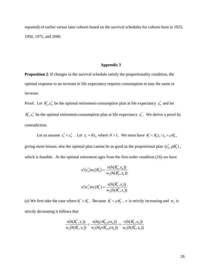
Appendix 3
Proposition 2: If changes in the survival schedule satisfy the proportionality condition, the
optimal response to an increase in life expectancy requires consumption to stay the same or
increase.
Proof. Let * *0,oR c be the optimal retirement-consumption plan at life expectancy *
0z and let
* *1 1,R c be the optimal retirement-consumption plan at life expectancy *
1z . We derive a proof by
contradiction.
Let us assume * *1 0c c< . Let 1 0z zθ= where 1θ > . We must have * * *
1 0 1 0 0/R R z z Rρ< = ,
giving more leisure, else the optimal plan cannot be as good as the proportional plan * *0 0( , )c pR ,
which is feasible. At the optimal retirement ages from the first-order condition (16) we have
** * 0 00 1 0 *
2 0 0
( ( , ))( ) ( )( ( , ))
v h R zu c w Rw h R z
′ =
** * 1 11 1 1 *
2 1 1
( ( , ))( ) ( )( ( , ))
v h R zu c w Rw h R z
′ =
(a) We first take the case where * *1 0R R≥ . Because * *
1 0R Rρ< , v is strictly increasing and 2w is
strictly decreasing it follows that
* **0 0 0 01 1
* * *2 1 1 2 0 0 2 0 0
( ( , )) ( ( , ))( ( , ))( ( , )) ( ( , )) ( ( , ))
v h R z v h R zv h R zw h R z w h R z w h R z
ρ ρρ ρ
< =
27
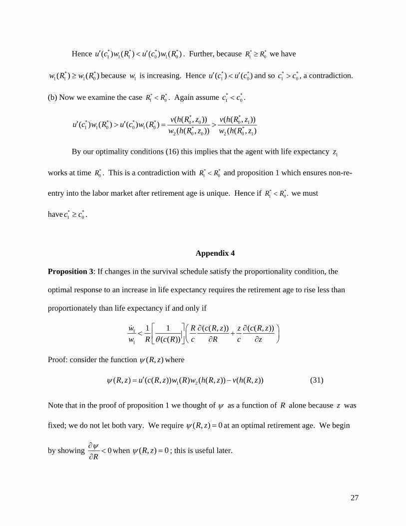
Hence * * * *1 1 1 0 1 0( ) ( ) ( ) ( )u c w R u c w R′ ′< . Further, because * *
1 0R R≥ we have
* *1 1 1 0( ) ( )w R w R≥ because 1w is increasing. Hence * *
1 0( ) ( )u c u c′ ′< and so * *1 0c c> , a contradiction.
(b) Now we examine the case * *1 0R R< . Again assume * *
1 0c c< .
* ** * * * 0 0 0 11 1 0 0 1 0 * *
2 0 0 2 0 1
( ( , )) ( ( , ))( ) ( ) ( ) ( )( ( , )) ( ( , )
v h R z v h R zu c w R u c w Rw h R z w h R z
′ ′> = >
By our optimality conditions (16) this implies that the agent with life expectancy 1z
works at time *0R . This is a contradiction with * *
1 0R R< and proposition 1 which ensures non-re-
entry into the labor market after retirement age is unique. Hence if * *1 0 .R R< we must
have * *1 0c c≥ .
Appendix 4
Proposition 3: If changes in the survival schedule satisfy the proportionality condition, the
optimal response to an increase in life expectancy requires the retirement age to rise less than
proportionately than life expectancy if and only if
1
1
1 1 ( ( , )) ( ( , ))( ( ))
w R c R z z c R zw R c R c R c zθ
⎡ ⎤ ∂ ∂⎛ ⎞< +⎜ ⎟⎢ ⎥ ∂ ∂⎝ ⎠⎣ ⎦
&
Proof: consider the function ( , )R zψ where
1 2( , ) ( ( , )) ( ) ( ( , )) ( ( , ))R z u c R z w R w h R z v h R zψ ′= − (31)
Note that in the proof of proposition 1 we thought of ψ as a function of R alone because z was
fixed; we do not let both vary. We require ( , ) 0R zψ = at an optimal retirement age. We begin
by showing 0Rψ∂
<∂
when ( , ) 0R zψ = ; this is useful later.
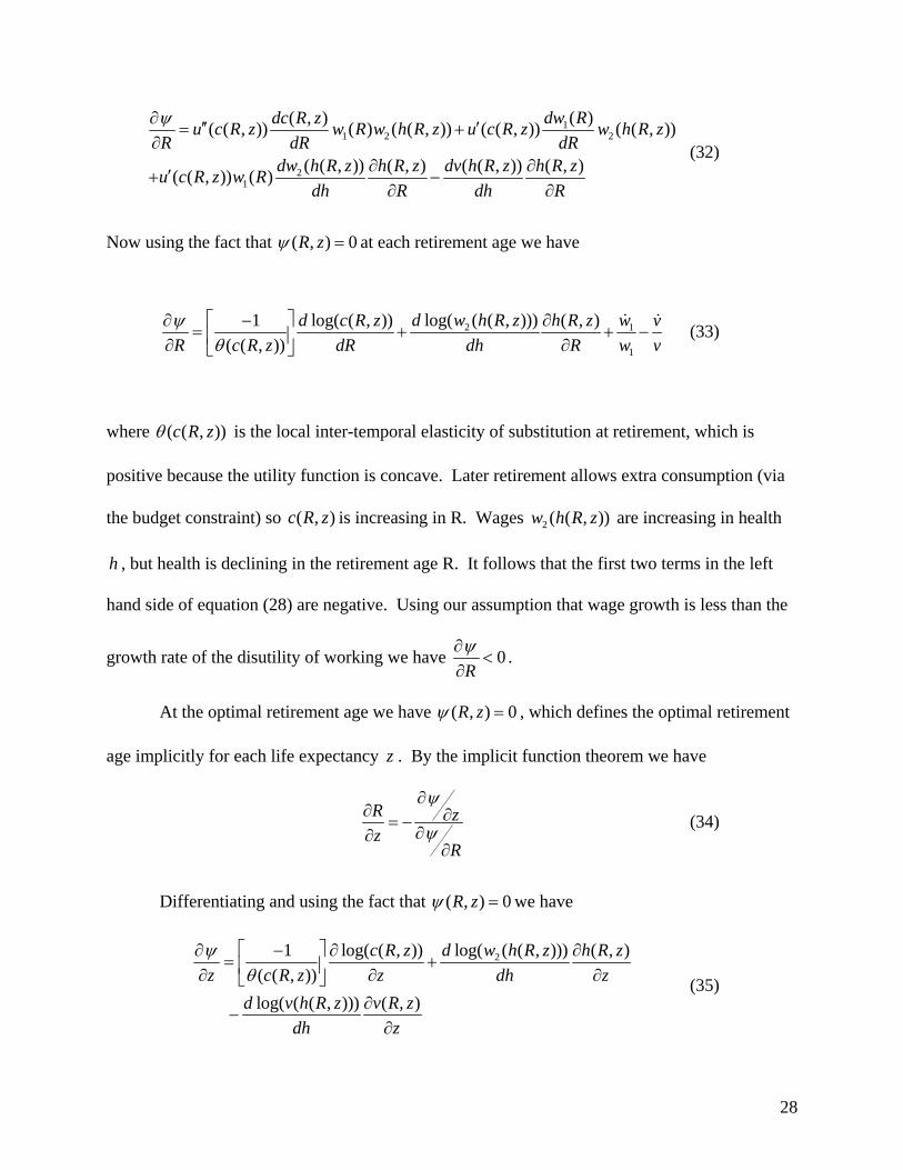
28
11 2 2
21
( )( , )( ( , )) ( ) ( ( , )) ( ( , )) ( ( , ))
( ( , )) ( , ) ( ( , )) ( , )( ( , )) ( )
dw Rdc R zu c R z w R w h R z u c R z w h R zR dR dR
dw h R z h R z dv h R z h R zu c R z w Rdh R dh R
ψ∂ ′′ ′= +∂
∂ ∂′+ −∂ ∂
(32)
Now using the fact that ( , ) 0R zψ = at each retirement age we have
2 1
1
log( ( ( , )))1 log( ( , )) ( , )( ( , ))
d w h R z wd c R z h R z vR c R z dR dh R w vψ
θ⎡ ⎤∂ − ∂
= + + −⎢ ⎥∂ ∂⎣ ⎦
& & (33)
where ( ( , ))c R zθ is the local inter-temporal elasticity of substitution at retirement, which is
positive because the utility function is concave. Later retirement allows extra consumption (via
the budget constraint) so ( , )c R z is increasing in R. Wages 2 ( ( , ))w h R z are increasing in health
h , but health is declining in the retirement age R. It follows that the first two terms in the left
hand side of equation (28) are negative. Using our assumption that wage growth is less than the
growth rate of the disutility of working we have 0Rψ∂
<∂
.
At the optimal retirement age we have ( , ) 0R zψ = , which defines the optimal retirement
age implicitly for each life expectancy z . By the implicit function theorem we have
R zz
R
ψ
ψ
∂∂ ∂= −
∂∂∂
(34)
Differentiating and using the fact that ( , ) 0R zψ = we have
2log( ( ( , )))1 log( ( , )) ( , )( ( , ))log( ( ( , ))) ( , )
d w h R zc R z h R zz c R z z dh z
d v h R z v R zdh z
ψθ⎡ ⎤∂ − ∂ ∂
= +⎢ ⎥∂ ∂ ∂⎣ ⎦∂
−∂
(35)

29
Now we have
1 1z R z z z Rz RR z RR
ψψ ψ
ψ
∂∂ ∂ ∂∂< ⇔ − < ⇔ − >∂ ∂∂∂
∂
(36)
where the reversal in the sign of the inequality comes from the fact that we have shown that
0Rψ∂
<∂
. Now note that ( , ) ( , )h t z h t zρ ρ = implies that h hR zR z∂ ∂
= −∂ ∂
. Hence we have
2
2 1
1
1
log( ( ( , )))1 log( ( , )) ( , ) log( ( ( , ))) ( , )( ( , ))
log( ( ( , )))1 log( ( , )) ( , ) log( ( ( , ))) ( , )( ( , ))
z RR z
d w h R zc R z h R z d v h R z v R zzc R z z dh z dh z
d w h R z wd c R z h R z d v h R z v R zRc R z dR dh R w dh R
θ
θ
∂< ⇔
∂⎛ ⎞⎡ ⎤− ∂ ∂ ∂
− + −⎜ ⎟⎢ ⎥ ∂ ∂ ∂⎣ ⎦⎝ ⎠⎛ ⎡ ⎤− ∂ ∂
> + + −⎜ ⎢ ⎥ ∂ ∂⎣ ⎦⎝
& ⎞⎟⎠
(37)
Applying h hR zR z∂ ∂
= −∂ ∂
we have
1
1
1 1 ( ( , )) 1 1 ( ( , ))1( ( )) ( ( ))
wz R c R z c R zz R RR z c R c z c R c R wθ θ
⎡ ⎤ ⎡ ⎤∂ ∂ − ∂< ⇔ > +⎢ ⎥ ⎢ ⎥∂ ∂ ∂⎣ ⎦ ⎣ ⎦
& (38)
1
1
1 1 ( ( , )) ( ( , ))1( ( ))
wz R R c R z z c R zR z w R c R c R c zθ
⎡ ⎤∂ ∂ ∂⎛ ⎞< ⇔ < +⎜ ⎟⎢ ⎥∂ ∂ ∂⎝ ⎠⎣ ⎦
& (39)
Appendix 5
Proposition 4: When the wage schedule rises the optimal response of the agent is to
(i) keep retirement unchanged and increase consumption proportionately with wages if the utility
function has a local inter-temporal elasticity of substitution of unity.
30
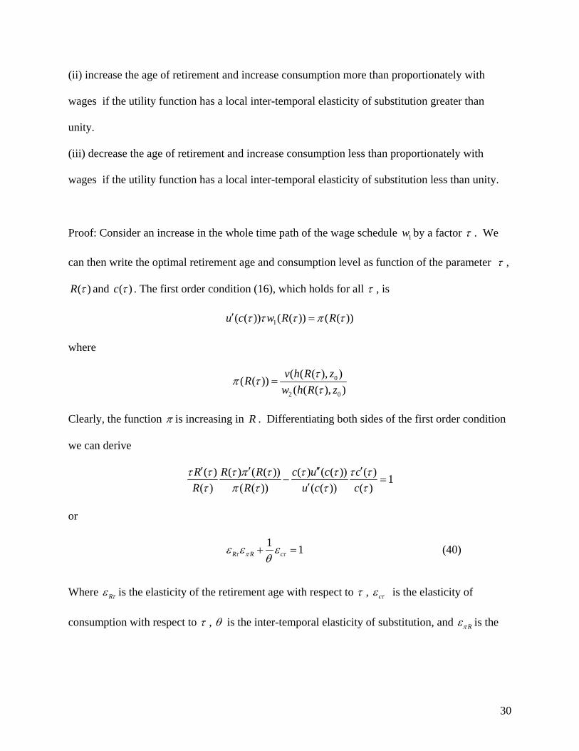
(ii) increase the age of retirement and increase consumption more than proportionately with
wages if the utility function has a local inter-temporal elasticity of substitution greater than
unity.
(iii) decrease the age of retirement and increase consumption less than proportionately with
wages if the utility function has a local inter-temporal elasticity of substitution less than unity.
Proof: Consider an increase in the whole time path of the wage schedule 1w by a factor τ . We
can then write the optimal retirement age and consumption level as function of the parameter τ ,
( )R τ and ( )c τ . The first order condition (16), which holds for all τ , is
1( ( )) ( ( )) ( ( ))u c w R Rτ τ τ π τ′ =
where
0
2 0
( ( ( ), )( ( ))( ( ( ), )
v h R zRw h R z
τπ ττ
=
Clearly, the function π is increasing in R . Differentiating both sides of the first order condition
we can derive
( ) ( ) ( ( )) ( ) ( ( )) ( ) 1( ) ( ( )) ( ( )) ( )
R R R c u c cR R u c cτ τ τ π τ τ τ τ τ
τ π τ τ τ′ ′ ′′ ′
− =′
or
1 1R R cτ π τε ε εθ
+ = (40)
Where Rτε is the elasticity of the retirement age with respect to τ , cτε is the elasticity of
consumption with respect to τ , θ is the inter-temporal elasticity of substitution, and Rπε is the

31
elasticity of π with respect to R , which we know to be positive. All these elasticities are local
though we suppress their dependence on consumption and age for convenience.
From the budget constraint given by equation (8) we have that the effect of increasing
wages by the proportion τ is
( )
1 20 0
( ) ( , ) ( , ) ( ) ( ( , ))RT
rt rtc e s t z dt e s t z w t w h t z dtτ
τ τ− −≤∫ ∫
It follows that changes to ( ) /c τ τ and ( )R τ have the same sign. Further, from this equation we
can derive:
1 01 01 0
c R
c R
c R
τ τ
τ τ
τ τ
ε εε εε ε
= ⇔ => ⇔ >< ⇔ <
Proposition 4 follows from these relationships and equation (40) .

32
References
Becker, G.S., T.J. Philipson, and R.R. Soares, 2005, “The Quantity of Life and the Evolution of
World Inequality,” American Economic Review 95: 277–91.
Bloom, D.E., D. Canning, and B. Graham, 2003, "Longevity and Life-Cycle Savings,"
Scandinavian Journal of Economics 105: 319–38.
Bloom, David E., David Canning, Rick Mansfield, and Michael Moore, 2007, “Demographic
Change, Social Security Systems, and Savings,” Journal of Monetary Economics 54: 92–114.
Bloom, David E., David Canning and Michael Moore, 2004, “The Effect of Improvements in
Health and Longevity on Optimal Retirement and Saving,” National Bureau of Economic
Research, Working Paper, No. 10919.
Carnes, B.A., Olshansky, S.J., and Grahn D, 2003, “Biological evidence for limits to the duration
of life,” Biogerontology 4: 31–45.
Chang, F-R., 1991, "Uncertain Lifetimes, Retirement, and Economic Welfare," Economica 58:
215–32.
Congressional Budget Office, 2004, The Outlook for Social Security, The Congress of the United
States, Washington D.C.

33
Costa, D. L., 1998a, The Evolution of Retirement: An American Economic History, 1880–1990,
National Bureau of Economic Research Series on Long-Term Factors in Economic
Development, University of Chicago Press, Chicago.
Costa, D. L., 1998b, "The Evolution of Retirement: Summary of a Research Project," American
Economic Review 88: 232–36.
Costa D.L., 2002, “Changing Chronic Disease Rates and Long-term Declines in Functional
Limitation Among Older Men,” Demography 39: 119-138.
Crimmins, E., Y. Saito, and D. Ingegneri, 1997, “Trends in disability-free life expectancy in the
United States, 1970–90,” Population Development Review 23: 555–572.
Cutler, David M., 2001, “Declining disability among the elderly,” Health Affairs 20 (6): 11–27.
Ehrlich, I., and H. Chuma, 1990, "A Model of the Demand for Longevity and the Value of Life
Extension," Journal of Political Economy 98: 761–82.
Feldstein, M.S., 1985, "The Optimal Level of Social Security Benefits," Quarterly Journal of
Economics 10: 303–20.
34
Fogel, R.W., 1994, "Economic Growth, Population Theory, and Physiology: The Bearing of
Long-Term Processes on the Making of Economic Policy," American Economic Review 84: 369–
95.
Fogel, R.W., 1997, "New Findings on Secular Trends in Nutrition and Mortality: Some
Implications for Population Theory," In M. Rosenzweig and O. Stark, eds., Handbook of
Population and Family Economics, vol. 1A, Elsevier, Amsterdam.
Fries, J.F., 1980, “Aging, natural death, and the compression of morbidity,” New England
Journal of Medicine 303:130-5.
Freedman, V.A., L.G. Martin, and R.F. Schoeni, 2002, “Recent trends in disability and
functioning among older adults in the United States: a systematic review,” Journal of the
American Medical Association 288: 3137–46.
Graham, Patrick, Tony Blakely, Peter Davis, Andrew Sporle and Neil Pearce, 2004,
“Compression, expansion, or dynamic equilibrium? The evolution of health expectancy in New
Zealand,” Journal of Epidemiology and Community Health 58: 659–666.
Gendell, M., 2001, “Retirement Age Declines Again in 1990s,” Monthly Labor Review (October)
12–21.
35
Gordo, Laura Romeu, 2006, “Compression of Morbidity and the Labor Supply of Older People,”
IAB Discussion Paper, No. 9/2006.
Gruber, J., and D. Wise, 1998, "Social Security and Retirement: An International Comparison,"
American Economic Review 88: 158–63.
Hamermesh, D.S., 1985, "Expectations, Life Expectancy, and Economic Behavior," Quarterly
Journal of Economics 10: 389–408.
Heckman, James J., 1976, “A Life Cycle Model of Earnings, Learning, and Consumption,”
Journal of Political Economy 84(4): S11-S44.
Hubbard, R Glenn and Judd, Kenneth L, 1987. "Social Security and Individual Welfare:
Precautionary Saving, Borrowing Constraints, and the Payroll Tax," American Economic Review
77(4): 630-46.
Kalemli-Ozcan, S., and D.N. Weil, 2002, "Mortality Change, the Uncertainty Effect, and
Retirement," Working Paper no. 8742, National Bureau of Economic Research, Cambridge,
MA.
Kotlikoff, L.J., A. Spivak, and L.H. Summers, 1982, “The Adequacy of Savings,” American
Economic Review 72(5):1056-69.

36
Laibson, D., 1998, "Life-Cycle Consumption and Hyperbolic Discount Functions," European
Economic Review 42: 861–71.
Laibson, D.I., A. Repetto, J. Tobacman, R.E. Hall, W.G. Gale, and G.A. Akerlof, 1998, "Self-
Control and Saving for Retirement," Brookings Papers on Economic Activity 1998: 91–196.
Lee, R., 2003, "The Demographic Transition: Three Centuries of Fundamental Change," Journal
of Economic Perspectives 17: 167–90.
Lee, R., and L. Carter, 1992, "Modeling and Forecasting U.S. Mortality," Journal of the
American Statistical Association 87: 659-671.
Lee, R., and J.R. Goldstein, 2003, “Rescaling the life cycle: Longevity and proportionality,”
Population and Development Review 29 (Supplement): 183–207.
Lee, Ronald, and Timothy Miller, 2001, “Evaluating the Performance of the Lee-Carter
Approach to Modeling and Forecasting Mortality,” Demography 38 (4): 537–549.
Manton, K.G., X. Gu, and V.L. Lamb, 2006, “Long-Term Trends in Life Expectancy and Active
Life Expectancy in the United States,” Population and Development Review 32(1): 81–105.
Mathers, C.D., R. Sadana, J.A. Salomon, C.J.L. Murray, and A.D. Lopez, 2001, "Healthy Life
Expectancy in 191 Countries, 1999," Lancet 357 (9269): 1685–91.

37
Mor, V., 2005, “The Compression of Morbidity Hypothesis: A Review of Research and
Prospects for the Future,” Journal of the American Geriatrics Society 53: S308–S309.
Nordhaus, W., 2003, “The Health of Nations: The Contribution of Improved Health to Living
Standards,” in Kevin H. Murphy and Robert H. Topel, eds., Measuring the Gains from Medical
Research: An Economic Approach, University of Chicago Press, Chicago.
Schultz, T.P., 1999, "Health and Schooling Investments in Africa," Journal of Economic
Perspectives 13: 367-88.
Skinner, J., 1985, "The Effect of Increased Longevity on Capital Accumulation," American
Economic Review 75: 1143–50.
Sydsaeter K., A. Strøm, and P. Berck, 2000, Economists’ Mathematical Manual, 3rd ed.,
Springer, Berlin.

38
Figure 1 Projected Survival Rates by Birth Year in the United States
0
10
20
30
40
50
60
70
80
90
100
0 10 20 30 40 50 60 70 80 90 100 110 120Age
Perc
ent S
urvi
ving
19001925195019752000
Source: Berkeley Mortality Database

39
Table 1
Testing the Proportionality Condition Relative to the 1900 Survival Schedule
Retirement
Age in
1900
Year of Survival Schedule
Year 1900 1925 1950 1975 2000
Life Expectancy at Age 16 50.7 56.4 59.6 61.8 63.5
Life Expectancy Relative to
1900 1.00 1.11 1.18 1.22 1.25
60 1.14 1.19 1.22 1.25 1.26
70 1.23 1.27 1.30 1.31 1.32
Initial Consumption- Wage Ratio with
retirement age proportional to life
expectancy
80 1.28 1.31 1.32 1.33 1.34
For each retirement age, the proportionality condition is satisfied if the initial consumption wage ratio under the new survival schedule, allowing for an increase in the retirement age proportional to the increase in life expectancy, is no smaller than that with the 1900 survival schedule.
Source: Berkeley Mortality Database and the authors' calculations.