A Theory of Rational Addiction

Gary S. Becker and Kevin M. Murphy (JPE, 1988)

Notes by Team Grossman (Spring 2015)

Meagan Madden and Mavzuna Turaeva

Contents Introduction ................................................................................................................................................... 2

Key Notation ................................................................................................................................................. 3

The Model ..................................................................................................................................................... 4

Dynamics ...................................................................................................................................................... 4

Adjacent Complementarity ........................................................................................................................... 8

Understanding Behaviors Related to Addictive Consumption ..................................................................... 9

Permanent Price Changes ......................................................................................................................... 9

Temporary Price Changes & Life Events ............................................................................................... 10

Cold Turkey & Binges ............................................................................................................................ 11

Claims that Addictive Behavior is Consistent with “Rationality” .......................................................... 12

Empirical Evidence ..................................................................................................................................... 13

Criticism ...................................................................................................................................................... 13

Extensions ................................................................................................................................................... 14

Summary & Conclusions ............................................................................................................................ 15

References ................................................................................................................................................... 15

Appendix ..................................................................................................................................................... 15

A1. Time Preference ............................................................................................................................... 15

A2. Control Problem & First Order Conditions ...................................................................................... 16

A3. Euler’s Equation ............................................................................................................................... 17

A4. Analytical Solution of the ODE ....................................................................................................... 18

A5. Condition for Adjacent Complementarity ........................................................................................ 18

Introduction The model of addiction by Becker and Murphy (B&M) (1998) was one of the first to model the behavior

of addicts in a “rational” way. By rational, they mean that addicts have stable preferences and make

utility-maximizing decisions about whether or not to consume an addictive good, and they are capable of

taking into account the consequences of the current consumption on the future. This approach differed

from previous models of addiction which assumed that addicts are “myopic” and heavily discount (or

ignore) utility/disutility in future periods.

B&M build on a few earlier economic models of tastes and addiction, including Stigler and Becker (1997)

and Iannaccone (1984, 1986). In “Rational Addiction,” B&M formalize the definition of an addictive

good as one where your consumption in one period is complementary to consumption in the next period

(i.e. adjacent complementarity). This definition encompasses addictions that are harmful or beneficial.

Therefore, we can think of many types of addictive goods in this model, including cigarettes, alcohol,

work, social media, food, and exercise.

In the B&M model, individuals choose between spending money on addictive goods and spending money

on all other goods. Addictive goods differ from other goods because utility from current consumption

depends on consumption in other periods, and these inter-temporal effects are contained in a “stock of

consumption” variable. To capture the change in this stock over time and how it affects your consumption

decision today, B&M develop a continuous time model. Instead choosing the optimal consumption bundle

to maximize utility subject to the budget (static case), individuals choose the optimal consumption paths

to maximize lifetime utility subject to the lifetime budget (dynamic case). An additional constraint in the

dynamic case is the flow of the stock variable.

From this dynamic model, B&M predict consumption patterns of addicts, including price responsiveness

in the short-run and long-run as well as binges and purges. There is strong empirical evidence to support

several aspects of the rational addiction model. However, critics still debate whether it is appropriate to

consider addicts in a rational thinking model.

Key Notation

Component Description

𝑐(𝑡) Consumption of an addictive good which is related to 𝑆(𝑡)

𝑦(𝑡) Consumption of a non-addictive good

𝑆(𝑡) “consumption stock” which is related to your consumption of addictive goods in

previous periods 𝑡 through “learning”

𝐷(𝑡) Expenditure on the endogenous depreciation of 𝑆 to “forget” your “consumption

stock” of addictive goods (e.g. rehabilitation costs)

�̇�(𝑡) Rate of change of 𝑆(𝑡) over time

𝐴0 Initial assets

𝑒−𝜎𝑡 Discount factor with constant rate of time preference 𝜎

𝑡 Time

𝑢(∙) Utility function a function of 𝑦, 𝑐, and 𝑆 (strongly concave in 𝑦, 𝑐 and 𝑆).

𝑟 Rate of interest, constant over time

𝑤(𝑆) Earnings as a concave function of the stock of consumption capital

𝑝(𝑡) Prices

𝑎(𝑡)

The shadow price of 𝑆, i.e. the marginal utility of an additional unit of

consumption stock 𝑆; also interpreted as the discounted utility and monetary

cost/benefit of additional consumption of 𝑐 through the effect on 𝑆.

Π𝑐(𝑡)

The shadow price of 𝑐(𝑡), i.e. the marginal utility of an additional of 𝑐(𝑡); also

interpreted as the full price of 𝑐(𝑡) which equals the sum of the market price of

𝑐(𝑡) plus the monetary value of the cost/benefit of future consumption

𝑉(∙) Lifetime indirect utility (i.e. the maximum obtainable utility)

𝜇 =𝜕𝑉

𝜕𝐴0 Shadow price of wealth; i.e. the marginal utility of an additional unit of wealth

𝛿 Rate of depreciation of the consumption stock which is constant

𝑘 “Composite constant” of indirect utility that depends on 𝐴0, 𝜇, 𝜎 (enters the

simplified dynamic optimization problem)

𝑆∗ Steady state value of 𝑆

The Model

Utility is derived from consumption of goods 𝑦 and addictive goods 𝑐 as well as the “stock of addictive

capital” 𝑆:

𝑢(𝑡) = 𝑢[𝑦(𝑡), 𝑐(𝑡), 𝑆(𝑡)] (1)

Utility is separable over time in 𝑦, 𝑐 and 𝑆, but not in 𝑦 and 𝑐 alone. This occurs because your “stock” 𝑆

depends on your past consumption of addictive goods 𝑐. Equation (1) implies that the amount that utility

you derive from consumption today partly depends on your “stock” which depends what you consumed in

previous periods. Investment in this “stock” occurs through the following function:

�̇�(𝑡) = 𝑐(𝑡) − 𝛿𝑆(𝑡) − ℎ[𝐷(𝑡)] (2)

Total lifetime utility is the discounted 𝑢(𝑡) evaluated over continuous time, with constant rate of time

preference 𝜎. (See A1 for more on time preferences)

𝑈(∙) = ∫ 𝑒−𝜎𝑡𝑢[𝑦(𝑡), 𝑐(𝑡), 𝑆(𝑡)]𝑑𝑡𝑇

0 (3)

The budget constraint says that consumption of all choice variables at prices 𝒑(𝑡) must be ≤ initial assets

(𝐴0) and future earnings to capital stock, 𝑤(𝑆(𝑡)). The budget is defined in present value terms using

interest rate 𝑟:

∫0

𝑇𝑒−𝑟𝑡[𝑦(𝑡) + 𝑝

𝑐(𝑡)𝑐(𝑡) + 𝑝

𝑑(𝑡)𝐷(𝑡)]𝑑𝑡 ≤ 𝐴0 + ∫

0

𝑇𝑒−𝑟𝑡𝑤(𝑆(𝑡))𝑑𝑡 (4)

Individuals want to choose the best consumption path in order to maximize their lifetime utility (3)

subject to their lifetime budget (4). This is basically a control problem with control variables 𝑐(𝑡), 𝑦(𝑡),

and 𝐷(𝑡); state variable 𝑆(𝑡), and the transition state function �̇�(𝑡). Using calculus of variations we setup

the Hamilton and derive the FOCs for an extrema (See A2 for formal derivations):

𝑢𝑦 = 𝜇𝑒(𝜎−𝑟)𝑡

ℎ𝑑(𝑡) ∙ 𝑎(𝑡) = 𝜇𝑝𝑑(𝑡)𝑒−𝑟𝑡 (5)

𝑢𝑐(𝑡) = 𝜇𝑝𝑐(𝑡)𝑒−(𝜎−𝑟)𝑡 − 𝑒𝜎𝑡𝑎(𝑡)

Where 𝑎(𝑡) and 𝜇 are the shadow price of consumption stock and wealth, respectively. These shadow

prices are interpreted at the marginal utility from small change in either stock or wealth.

Dynamics The solution to the dynamic optimization problem is a differential equation which determines the optimal

consumption path of 𝑐 and 𝑦 and state transition path of 𝑆. To more easily find the solution, B&M

simplify the model and then find the analytical and graphical solution to the differential equation.

Simplifying Assumptions:

a. Infinite time: 𝑇 = ∞

b. Time preference equals interest rate: 𝜎 = 𝑟

c. No endogenous depreciation of 𝑆: 𝐷(𝑡) = 0

d. Quadratic utility and earnings functions, so the relationship between 𝑐 and 𝑆 is linear.

Since B&M are most interested in the dynamics of 𝑐 and 𝑆, they optimize 𝑦 out of the value function.

Essentially, this allows them to examine small deviations of 𝑐 and 𝑆 near the steady-states and easily

represent the dynamics of these variables of interest using a two-dimensional phase diagram. Therefore,

the value function is expressed as a quadratic of only 𝑐 and 𝑆 through a Taylor Series Expansion:

𝐹(𝑡) = 𝛼𝑐𝑐(𝑡) + 𝛼𝑠𝑆(𝑡) +𝛼𝑐𝑐

2[𝑐(𝑡)]2 +

𝛼𝑠𝑠

2[𝑆(𝑡)]2 + 𝛼𝑐𝑠𝑐(𝑡)𝑆(𝑡) − 𝜇𝑝𝑐𝑐(𝑡) (6)

Where the coefficients 𝛼𝑠 and 𝛼𝑠𝑠 contain the marginal and secondary effects of 𝑆 on the utility function

(𝑢) and the earnings function (𝑤). The table below depicts the first- and second-order conditions for the

case of harmful goods and the case of beneficial goods.

Type FOCs Notation in (6) Description Second

Order Notation in (6)

Harmful

addictive

goods

𝑢𝑠 < 0 𝜕𝐹

𝜕𝑆= 𝛼𝑠 < 0

Adverse effect on utility from an increase

in “consumption stock” of a harmful

addictive good 𝑢𝑠𝑠 < 0

𝜕2𝐹

𝜕𝑆2= 𝛼𝑠𝑠 < 0

𝑤𝑠 < 0 Adverse effect on earnings from an

increase in “consumption stock” of a

harmful addictive good 𝑤𝑠𝑠 < 0

Beneficial

addictive

goods

𝑢𝑠 > 0 𝜕𝐹

𝜕𝑆= 𝛼𝑠 > 0

Positive effect on utility from

“consumption stock” of beneficial

addictive good 𝑢𝑠𝑠 < 0

𝜕2𝐹

𝜕𝑆2= 𝛼𝑠𝑠 < 0

𝑤𝑠 > 0 Positive effect on earnings from

“consumption stock” of beneficial

addictive good 𝑤𝑠𝑠 < 0

For all

“addictive”

goods

𝑢𝑐 > 0 𝜕𝐹

𝜕𝑐= 𝛼𝑐 > 0

⟹Utility from consumption of addictive

goods is increasing, but at a decreasing

rate

⟹ 𝑢𝑐𝑠 > 0 is the key element of the

model which indicates complementarity

of the consumption and capital stock; this

means that the marginal utility of current

consumption of an addictive good

increases with past consumption of 𝑐‡

𝑢𝑐𝑐 < 0 𝜕2𝐹

𝜕𝑐2= 𝛼𝑐𝑐 < 0

𝑢𝑐𝑠 > 0 𝜕2𝐹

𝜕𝑐𝜕𝑆= 𝛼𝑐𝑠 > 0

‡Alternatively, 𝑢𝑐𝑠 < 0 means 𝑐 and 𝑆 are substitutes, and 𝑢𝑐𝑠 = 0 means 𝑐 and 𝑆 are not related. Under these

conditions 𝑐 is non-addictive.

The value function (6) gives the instantaneous indirect utility of your consumption choices (𝑐, 𝑆) in time

𝑡. Individuals want to maximize instantaneous utility over all time, so the indirect lifetime utility from this

maximization problem is given by

𝑉(𝐴0, 𝑆0, 𝑝𝑐) = 𝑘 + max𝑐,𝑆 ∫0

∞𝑒−𝜎𝑡𝐹[𝑆(𝑡), 𝑐(𝑡)]𝑑𝑡 (7)

In (7), 𝑘 is a constant utility value that is a function of 𝐴0, 𝜇2, the 𝜎 discount factor on 𝑦, plus the

coefficients for 𝑦 in the quadratic utility function (i.e. the coefficients before B&M optimized out 𝑦).

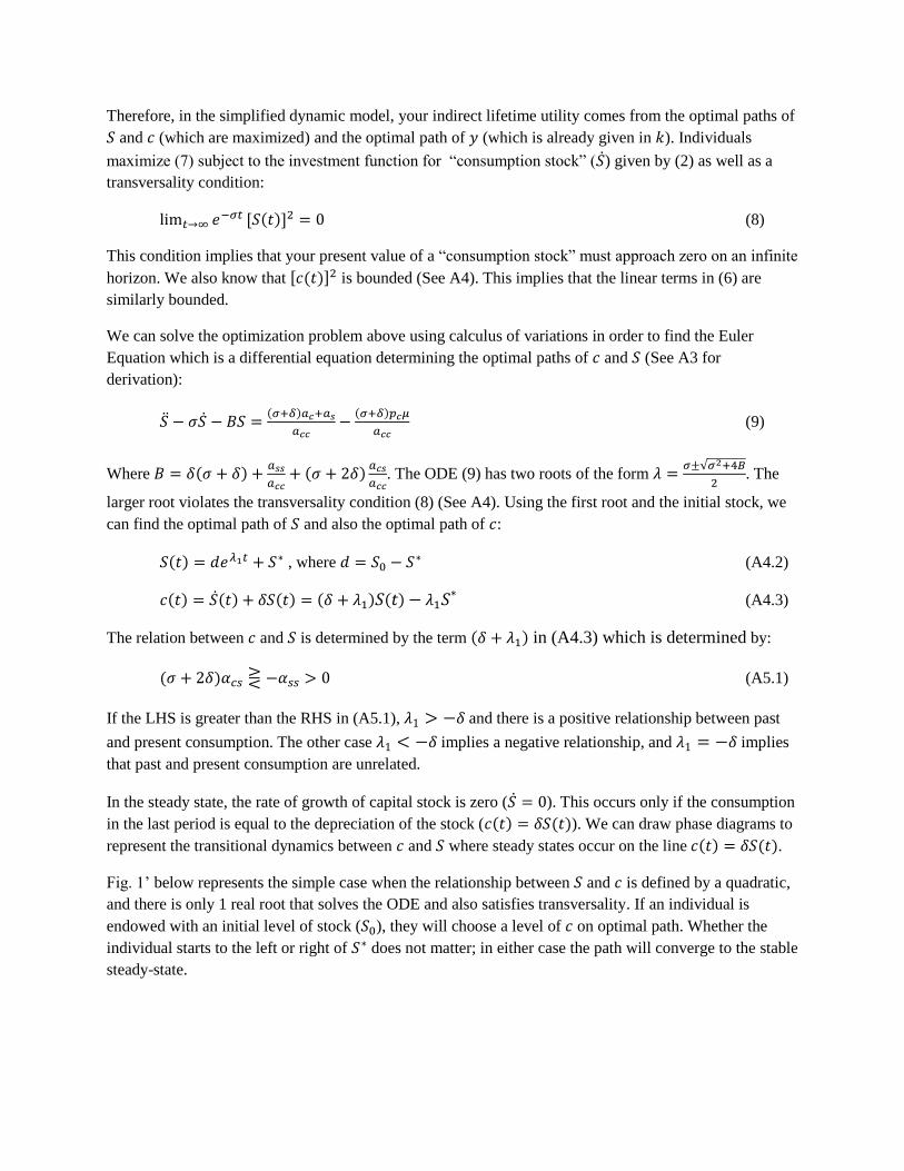
Therefore, in the simplified dynamic model, your indirect lifetime utility comes from the optimal paths of

𝑆 and 𝑐 (which are maximized) and the optimal path of 𝑦 (which is already given in 𝑘). Individuals

maximize (7) subject to the investment function for “consumption stock” (�̇�) given by (2) as well as a

transversality condition:

lim𝑡→∞ 𝑒−𝜎𝑡 [𝑆(𝑡)]2 = 0 (8)

This condition implies that your present value of a “consumption stock” must approach zero on an infinite

horizon. We also know that [𝑐(𝑡)]2 is bounded (See A4). This implies that the linear terms in (6) are

similarly bounded.

We can solve the optimization problem above using calculus of variations in order to find the Euler

Equation which is a differential equation determining the optimal paths of 𝑐 and 𝑆 (See A3 for

derivation):

�̈� − 𝜎�̇� − 𝐵𝑆 =(𝜎+𝛿)𝑎𝑐+𝑎𝑠

𝑎𝑐𝑐−

(𝜎+𝛿)𝑝𝑐𝜇

𝑎𝑐𝑐 (9)

Where 𝐵 = 𝛿(𝜎 + 𝛿) +𝑎𝑠𝑠

𝑎𝑐𝑐+ (𝜎 + 2𝛿)

𝑎𝑐𝑠

𝑎𝑐𝑐. The ODE (9) has two roots of the form 𝜆 =

𝜎±√𝜎2+4𝐵

2. The

larger root violates the transversality condition (8) (See A4). Using the first root and the initial stock, we

can find the optimal path of 𝑆 and also the optimal path of 𝑐:

𝑆(𝑡) = 𝑑𝑒𝜆1𝑡 + 𝑆∗ , where 𝑑 = 𝑆0 − 𝑆∗ (A4.2)

𝑐(𝑡) = �̇�(𝑡) + 𝛿𝑆(𝑡) = (𝛿 + 𝜆1)𝑆(𝑡) − 𝜆1𝑆∗ (A4.3)

The relation between 𝑐 and 𝑆 is determined by the term (𝛿 + 𝜆1) in (A4.3) which is determined by:

(𝜎 + 2𝛿)𝛼𝑐𝑠 ⋛ −𝛼𝑠𝑠 > 0 (A5.1)

If the LHS is greater than the RHS in (A5.1), 𝜆1 > −𝛿 and there is a positive relationship between past

and present consumption. The other case 𝜆1 < −𝛿 implies a negative relationship, and 𝜆1 = −𝛿 implies

that past and present consumption are unrelated.

In the steady state, the rate of growth of capital stock is zero (�̇� = 0). This occurs only if the consumption

in the last period is equal to the depreciation of the stock (𝑐(𝑡) = 𝛿𝑆(𝑡)). We can draw phase diagrams to

represent the transitional dynamics between 𝑐 and 𝑆 where steady states occur on the line 𝑐(𝑡) = 𝛿𝑆(𝑡).

Fig. 1’ below represents the simple case when the relationship between 𝑆 and 𝑐 is defined by a quadratic,

and there is only 1 real root that solves the ODE and also satisfies transversality. If an individual is

endowed with an initial level of stock (𝑆0), they will choose a level of 𝑐 on optimal path. Whether the

individual starts to the left or right of 𝑆∗ does not matter; in either case the path will converge to the stable

steady-state.

With a different form for 𝐹(𝑡), the solution will be different and other phase diagrams are possible,

including multiple steady states, unsteady states, and jumps (See Fig. 1)

In Fig. 1, there are two steady states along the optimal path of the capital stock; one is stable and one is

unstable. The optimal path line 𝑠1 has stable steady state at 𝛿𝑆∗1 = 𝑐∗1. But the optimal path line 𝑠0 has

an unstable steady state at 𝛿𝑆∗0 = 𝑐∗0. The line 𝑠0 cuts cuts the steady-state line from below.

An increase in parameters 𝜎, 𝛿, or 𝑎𝑐𝑠, will increase the degree of adjacent complementarity, which in

turn makes the smaller root 𝜆1 large in algebraic value. The roots 𝜆1 and 𝜆2 will be positive when

adjacent complementarity is strong enough to make 𝐵 < 0 (See A5.) This makes the steady state

unstable: consumption grows over time if initial consumption exceeds the steady state level, and it falls to

zero when initial consumption is below the steady state level.

The unstable state is crucial in understanding of rational addictive behavior. An increase in the degree of

potential addiction (i.e. the degree of complementarity 𝑎𝑐𝑠) raises the likelihood that the steady state is

unstable. Thus, unstable steady states can explain rational “pathological” addictions, in which the

consumption of a good increases over time, even though the person fully anticipates future and his/her

rate of time preference is no smaller than the rate of interest. The unstable steady state also helps in

explain “normal” addictions that may involve rapid increases in consumption only for a while.

With two steady states relatively few people consistently consume small quantities of addictive goods.

Consumption diverges from the unstable steady state either to zero or to a high level. Empirically, the

distribution of consumption of highly addictive goods tends to be bimodal: people either consume a lot of

it or very little (e.g. cigarettes or cocaine). On the other hand, alcohol consumption is not as addictive as

nicotine or cocaine (for most people), so the distribution of alcohol consumption is more continuous.

Adjacent Complementarity Adjacent complementarity is the determining condition for addiction under rational addiction theory. For

a good to be addictive, the consumption in adjacent periods must be complementarity. Mathematically,

(𝜎 + 2𝛿)𝛼𝑐𝑠 > −𝛼𝑠𝑠 > 0 (See A5). The parameter 𝛼𝑐𝑠 > 0 is interpreted as the degree of

complementarity.

The concept of adjacent complementarity is closely related to the idea of reinforcement: that greater

current consumption raises future consumption. Tolerance means that given levels of consumption are

less satisfying when past consumption has been greater. Harmful addictions imply a form of tolerance

because higher past consumption of harmful goods lowers present utility from the same level of

consumption. B&M argue that the effect of tolerance exists only for harmful goods. For example, there is

biological evidence of developing tolerance to drugs; after using drugs for a while, you do not receive the

same “high” from the same amount of consumption. However, we think you can also develop a tolerance

to beneficial addiction (e.g. runner’s “high”).

We see that different individuals have different addictions, and an inidividual may be addictive to some

goods but not other. The parameters in the model (𝜎,𝛿, plus all the 𝛼 coefficients from (6)), determine the

“addictiveness” of a good, and these parameters are different by person. For example, present-oriented

individuals are potentially more addicted to harmful goods than future oriented individuals. The reason is

that an increase in past consumption leads to a smaller rise in full price when the future is more heavility

dicsounted. The folloing diagram captures the dynamics of consumption of the addictive good related to

individually-determined parameters:

Understanding Behaviors Related to Addictive Consumption

Permanent Price Changes

B&M derive the own-price effect on demand for addictive goods, then take the partial derivative with

respect to time:

𝜕

𝜕𝑡[

𝜕𝑐(𝑡)

𝜕𝑝𝑐] =

𝜕𝑐̇

𝜕𝑝𝑐=

𝜕

𝜕𝑝𝑐(

𝑑𝑐

𝑑𝑆�̇�) =

𝑑𝑐

𝑑𝑆

𝜕�̇�

𝜕𝑝𝑐+ �̇�

𝜕

𝜕𝑝𝑐(

𝑑𝑐

𝑑𝑆) (10)

In the steady-state �̇� = 0, so the term �̇�𝜕

𝜕𝑝𝑐(

𝑑𝑐

𝑑𝑆) ≈ 0 near the steady-state. Therefore,

𝜕

𝜕𝑡[

𝜕𝑐(𝑡)

𝜕𝑝𝑐] ≈

𝑑𝑐

𝑑𝑆

𝜕�̇�

𝜕𝑝𝑐 (11)

The term 𝜕�̇�

𝜕𝑝𝑐 is necessarily negative because

𝜕𝑐

𝜕𝑝𝑐< 0 (assuming normal goods), and �̇� depends on 𝑐.

Therefore, the sign of 𝜕

𝜕𝑡[

𝜕𝑐(𝑡)

𝜕𝑝𝑐] is determined by

𝑑𝑐

𝑑𝑆. If past and present consumption are complements,

𝑑𝑐

𝑑𝑆> 0 and the effect of a price change increases over time.

Furthermore, B&M show that the long-term effect of price is often greater for more addictive goods. In

the first case, assuming the quadratic form of 𝐹(𝑡) (6), the derivative of the FOCs yields:

𝑑𝑐∗

𝑑𝑝𝑐

=𝜇

𝑎𝑐𝑐

𝛿(𝜎+𝛿)

𝐵< 0 (12)

The degree of addiction (𝛼𝑐𝑆) lowers B in the denominator of (12), so that the change in steady state

consumption w.r.t to price is greater for highly addictive goods.

Assuming another form on (6) could result in unsteady states which would further amplify the effect of

price changes on consumption. B&M depict this in Fig. 2 with the curves 𝑝1𝑝1 and 𝑝2𝑝2 which have

unstable steady states at 𝑆1∗ and 𝑆2∗, respectively. If your initial stock under 𝑝1 is to the left of 𝑆1∗, then

you will move toward zero consumption. If your initial stock under 𝑝2 is to the right of 𝑆2∗, then you will

move to the steady state of consumption where there is high stock and high consumption. Therefore, if

your initial stock is between 𝑆1∗ and 𝑆2∗ and prices drop from 𝑝1 to 𝑝2, then your steady state will

change. The effect of the price change moves your steady state value of consumption from zero to a much

higher level of 𝑐.

B&M similarly derive the effect of wealth on steady state consumption by taking the derivative of the

FOCs with respect to the marginal utility of wealth (𝜇):

𝑑𝑐∗

𝑑𝜇=

𝛿

𝑎𝑐𝑐𝐵[(𝜎 + 𝛿)𝑝𝑐 −

𝑑𝑎𝑠

𝑑𝜇] (13)

We can define the addictive good as inferior or superior by the sign 𝑑𝑐∗

𝑑𝜇≶ 0. The direction of the

inequality depends partly on how your earnings function 𝑤(𝑆) is affected by consumption. B&M suggest

that harmful goods are more likely to be inferior because the productivity loss associated with addiction is

greater for high paying jobs.

Temporary Price Changes & Life Events

The effects of past and future prices are not symmetric. B&M model this with an additional exponential

discount factor in terms of future time 𝜏 (See the last line of A3). At time 𝑡, the utility discounting on

future periods is 𝑒−(𝜎+𝛿)(𝜏−𝑡), compared to the utility discounting of past periods 𝑒−(𝜎+𝛿)𝑡.

The effect of a small, temporary change in price has a non-zero limit as the length of time → 0. B&M

give the limits as:

𝑑𝑐(𝑡)

𝑑𝑝(𝜏)=

(𝛿+𝜆1)𝑒−𝜆2𝜏

𝑎𝑐𝑐(𝜆2−𝜆1)[(𝛿 + 𝜆2)𝑒𝜆2𝑡 − (𝛿 + 𝜆1)𝑒𝜆1𝑡], 𝜏 > 𝑡 (14)

𝑑𝑐(𝑡)

𝑑𝑝(𝜏)=

(𝛿+𝜆1)𝑒𝜆1𝑡

𝑎𝑐𝑐(𝜆2−𝜆1)[(𝛿 + 𝜆2)𝑒−𝜆1𝜏 − (𝛿 + 𝜆1)𝑒−𝜆2𝜏], 𝑡 > 𝜏 (15)

(14) and (15) imply that the cross-price effects (across time periods) depend on (𝛿 + 𝜆1). We show in A5

that (𝛿 + 𝜆1) > 0 means that consumption of a good in different time periods are adjacent complements.

Therefore, the cross-price effects (14) and (15) are negative when 𝑐(𝑡) and 𝑐(𝑡 + 1) are complementary.

This responsiveness to future prices is the key difference to distinguish “rational addicts” from “myopic”.

B&M also suggest that adjacent complements are similar to “complementarity in the Slutsky sense”

(somewhat contradicting Ryder and Heal).

The negative cross-price effects associated with complementary goods are greater when the degree of

addiction is higher or the anticipation of price changes is longer. This effect is amplified when steady

states can be unstable because small changes in price can lead to different steady states with very different

levels of consumption (See Fig. 2).

These temporary changes in price effect consumption only in the current period. On the other hand,

permanent changes affect the price in all future periods, which leads to further reduction of current period

consumption. Thus, the SR price responsiveness is smaller than in the LR.

B&M extend the idea of temporary price changes to temporary life events that stimulate addiction (e.g.

divorce, unemployment, death of friend, etc) by increasing the marginal utility of addictive consumption

but lowering total utility. B&M address the critics of utility (“happiness”)-maximization saying,

“Although our model does assume that addicts are rational and maximize utility, they would not be happy

if their addiction results from anxiety-raising events, such as death or divorce, that lower their utility. […]

However, they would be even more unhappy if they were prevented from consuming addictive goods.”

Cold Turkey & Binges

B&M describe this empirically observed behavior with Fig.2: 𝑐 > 𝛿�̂� when 𝑆 > �̂�, and 𝑐 < 𝛿�̂� when

𝑆 < �̂�. Here, �̂� is not a steady-state stock, but it plays a role similar to unstable steady-state stock when

the utility function is concave (Figure 1). A slight deviation from �̂� leads to drastic change in

consumption, either to zero or along the upper part of the 𝑝𝑠 curve. This is the “cold turkey” mechanism

at work around �̂�. Once decided the addict will stop consuming immediately.

The explanation of such discontinuity is as follows: If 𝑆 is even slightly bigger compared to �̂�, the optimal

consumption plan calls for high 𝑐 in the future because the good is highly addictive. Strong

complementarity between present and future consumption then requires a high level of current 𝑐. If 𝑆 is

even slightly below �̂�, then future consumption will be very low by strong complementarity. We call �̂�

the “hooking” point.

Claims that Addictive Behavior is Consistent with “Rationality”

Behavior Explanation Algebraic

presentation

Theoretical and/or Empirical

Justification

Myopia

Concept of rationality does

not rule out strong discount

of future events

𝜎 → ∞ (if 𝜎 = 𝑟) so

𝑎(𝑡) → 0

Fully myopic (𝜎 = ∞) behavior is

formally consistent with the model

and, therefore “rational”

Myopia with old

age

Old people are “rationally”

myopic and more likely to

be addicted

1

𝑡= 𝜎 – approximation

of time preference

Even with high (theoretical) rate of

time preference, empirically, they are

usually not addicts (B&M attribute to

poor health and selection in the type

of people who live to old age)

Cold Turkey

Rational addiction theory

implies that highly

addictive goods require

cold turkey to quit because

the strong degree of

complementarity means the

consumption path is

discontinuous

𝜆 =𝜎 ± √𝜎2 + 4𝐵

2

Both roots are complex,

when 4𝐵 < −𝜎2

Implies sharp swings in consumption

are possible in response to “small”

changes in the price

Ending addiction

regardless of

short-run “pain”

Rational to exchange a

large short-term loss in

utility for an even larger

long-term gain

𝜕𝑈

𝜕𝑐> 0 implies utility

loss from withdrawal; 𝜕𝑈

𝜕𝑆< 0 implies long-

run gain from

subsequently lower 𝑆

Addicts are actually forward-looking

Addict’s

difficulty quitting

An individual’s weak will

and limited self-control in

their attempt to quit does

not imply they are

irrational. It may take trial

and error to find the best

option to reduce the short-

run loss in utility from

withdrawals.

Similar argument as

above

Addicts are utility maximizers and

searching for the best way to reduce

pains associated with withdrawal.

Overeating This is not a prototype of

irrational behavior.

Suppose a weight stock

(𝑆𝑤), eating capital

stock (𝑆𝑒), and rates of

depreciation (𝛿𝑤, 𝛿𝑒):

𝛼𝑐𝑠𝑤< 0 , 𝛼𝑐𝑠𝑒

> 0 ;

𝛿𝑒 > 𝛿𝑤,

⟹ 𝑆�̇� > 𝑆�̇�

Cycles of overeating and dieting

possible: After increase in 𝑆𝑒, eating

levels off and begins to fall so that

weight stock falls. When weight is

sufficiently low, eating picks up the

cycle starts again.

Binges

Just like overeating, binges

are not an inconsistent

behavior.

Could think of similar

stocks related to

drinking: “social stock”

and “productivity

stock”

Similar to overeating case: cycles can

be the outcome of consistent

maximization over time, recognizing

that the effect of increased current

drinking/socializing, on both future

productivity and the desire to drink

more in the future.

Empirical Evidence Within the paper B&M cite some empirical evidence to give credence to their model. For example, they

include empirical measures of price elasticity for cigarettes. They also cite long-term changes in smoking

behavior after the full-price of cigarettes changed with new health warnings from the Surgeon General.

Since B&M, the literature of economic theory and empirical microeconomic research on addiction has

greatly expanded. The economic framework for modeling addictive behaviors has contributed to the

cross- and inter-disciplinary subject of addiction. “Rational Addiction” now has more than 3000 citations

in Google Scholar.

The theoretical model of rational addiction “has been reinforced by a sizable empirical literature, […]

which has tested and generally supported the key empirical contention of the Becker and Murphy model:

that the consumption of addictive goods today will depend not only on past consumption but on future

consumption as well. More specifically, this literature has generally assessed whether higher prices next

year lead to lower consumption today, as would be expected with forward-looking addicts. The fairly

consistent findings across a variety of papers that this is the case has led to the acceptance of this

framework for modeling addiction.” (Gruber and Köszegi, 2001).

Becker, Grossman and Murphy (1994) were the among the first to empirically test “rational addiction”

with cigarette prices and consumption. They observed a negative cross-price effect of future prices on

current consumption of cigarettes, and found greater long-run price elasticity compared to the short-run.

Similarly, Gruber and Köszegi (2001) found empirical evidence of forward-looking cigarette smokers.

They estimated the consumption response to state excise taxes that have been legislated but not yet

implemented. They also extend the theoretical model of B&M with hyperbolic discounting, which

delivers the same theoretical predictions as the rational addiction model. Empirically, most of the tests of

rational addiction are not robust to the possibility of hyperbolic discounting.

Wang (2014) modeled smoking behavior as a dynamic discrete choice model, where smokers decide

whether to smoke or quit in each period based on their health, income, survival probability, and state

transition functions. They estimate the discount factor with maximum likelihood and find β close to 1,

which indicates that smokers are forward-looking in their behavior.

Criticism

Hyperbolic Discounting

B&M assume time consistent discounting, and this assumption generated much criticism. The basis of

this criticism comes from the overwhelming psychological evidence that humans are time-inconsistent.

This means that the relative valuation of utilities in the near future is different compared to the relative

valuation of utilities in the far future. George Ainslie’s works, Picoeconomics (1992) and Breakdown of

Will (2001) are often cited in this regard. However, Gruber and Koszegi (2001) extend the rational

addiction model with hyperbolic discounting and find that many of the implications are the same.

However, optimal taxation of harmful addictive goods does differ if addicts are actually hyperbolic

discounters.

“The Dangers in Analogical Thinking” & Misapplied Math

Other critics argue that “rational” modeling of addiction is an absurd approach and inappropriate

application of math. Elster (1997) is a strong critic of rational addiction theory. B&M model increasing

rate of time discounting and assume that an addict’s “awareness of the future consequences is not

impaired.” Elster maintains that addicts often cannot make rational, utility-maximizing decisions about

the future because addictions (e.g. mind-altering drugs) impair judgment.

Rogeberg (2004) also takes a stab at B&M’s claim of rational addiction behavior. He argues that the

application of “rational thinking” economic theory to addiction is “absurd,” and that this is an

inappropriate use of math to defend a theory. Similar to Elster, the main assumption of contention for

Rogeberg is that addicts make detailed and forward-looking plans.

We think that these types of criticism may qualify B&M’s theory for certain addictive substances that

seriously affect judgment (e.g some types of illicit drugs). However, the case can be made that “Rational

Addiction” applies to many other addictions that do not affect decision-making, although they may have

real physiological effects. For example, you can become addicted to a caffeine buzz, but coffee does not

affect your ability to make rational, forward-thinking decisions. In fact, most coffee-drinkers think that

caffeine improves their brain function and focus!

Extensions

For simplicity in the dynamic analysis, B&M assume that ℎ[𝐷(𝑡)] = 0, but we think that 𝐷(𝑡) might be a

choice variable of interest. B&M call 𝐷(𝑡) “expenditures on endogenous depreciation or appreciation.”

Then, ℎ[𝐷(𝑡)] enters the state transition function �̇�(𝑡) = 𝑐(𝑡) − 𝛿𝑆(𝑡) − ℎ[𝐷(𝑡)]. If your consumption

stock of addictive goods comes from “learning” from past consumption, we can think of 𝐷(𝑡) as

expenditures that help you “forget” your past consumption. For example, you might spend money on

rehabilitation or new hobbies in order to reduce the effect of your stock on future consumption. We will

presume that all expenditures 𝐷 fight addiction that ℎ is a monotonic function of 𝐷.

With 𝐷(𝑡) remaining in the model, the Taylor Series Expansion from (6) contains terms for the partial

effects of 𝐷 through 𝑆, as well as the linear term for the price of 𝐷:

𝐹(𝑡) = 𝛼𝑐𝑐(𝑡) + 𝛼𝑆𝑆(𝑡) +𝛼𝑐𝑐

2[𝑐(𝑡)]2 +

𝛼𝑆𝑆

2[𝑆(𝑡)]2 + 𝛼𝑐𝑆𝑐(𝑡)𝑆(𝑡) + 𝜶𝑺𝑫𝑺(𝒕)𝑫(𝒕) − 𝜇𝑝𝑐𝑐(𝑡) − 𝝁𝒑𝑫𝑫(𝒕) (16)

Now, we suggest the condition for adjacent complementarity becomes:

(𝜎 + 2𝛿)𝛼𝑐𝑆′ > −(𝛼𝑆𝑆 + 𝛼𝑆𝐷) > 0 (17)

As before, 𝛼𝑆𝑆 < 0, and now we assume 𝛼𝑆𝐷 < 0. Thus, in order for the adjacent complementarity to

hold with additional anti-addiction measures, 𝛼𝑐𝑆′ must be very large. This makes intuitive sense, that a

strong addiction would require more resources to defeat. More interesting questions involve the optimal

path of 𝐷(𝑡) and how it relates to different types of addiction (with different degrees of 𝛼𝑐𝑆′). One could

solve the dynamic optimization problem with the value function (16) to derive the optimal path of 𝑐(𝑡),

𝑦(𝑡), 𝑆(𝑡), and 𝐷(𝑡).

Summary & Conclusions Becker and Murphy develop a model of addiction that hinges on the relationship between past and present

consumption of an addictive good. Consumption in different periods is related by a “stock” variable 𝑆.

They derive the optimal paths of “consumption stock” 𝑆(𝑡) and consumption 𝑐(𝑡), and then compare the

dynamics of 𝑐 and 𝑆 near the steady-state. They find this dynamic model of forward-thinking addicts is

consistent with many stylized facts and empirically-testable behaviors of addiction, such as price

responsiveness, the increased consumption with stressful life events, binges, purges, and cold-turkey

quitting. The body of empirical work, mostly related to smoking and drinking, gives strong support for

B&M’s rational addiction model.

References Barro, Robert J. and Xavier Sala-i-Martin. 2004. Economic Growth, Second Edition. Cambridge, MA:

The MIT Press.

Becker, Gary S. and Kevin M. Murphy. 1988. A theory of rational addiction. Journal of Political

Economy 96(4): 675-700.

Becker, Gary S., Michael Grossman, and Kevin M. Murphy. 2994. An empirical analysis of cigarette

addiction. The American Economic Review. 84(3):396-418.

Elster, Jon. 1997. More than enough. The University of Chicago Law Review, 64(2), 749-764.

Gruber, Jonathan and Botond Köszegi. 2001. Is addiction “rational”? Theory and evidence. The Quarterly

Journal of Economics 116(4): 1261-1303.

Rogeberg, Ole. 2004. Taking absurd theories seriously: Economics and the case of rational addiction

theories. Philosophy of Science, 71(3), 263-285. < http://www.jstor.org/stable/10.1086/421535 >.

Qin, Wei. 2012. Hyperbolic discounting. < http://tinyurl.com/p2fp9qg >.

Wang, Yang. 2014. Dynamic implications of subjective expectations: Evidence from adult smokers.

American Economic Journal: Applied Econometrics 6(1): 1-37.

Appendix

A1. Time Preference

Individuals discount utility from future periods, and there is empirical evidence of different types and

magnitudes of discounting behavior. In essence, time preference reflects a person’s lack of foresight or

self-control. Theoretical models with multiple periods (or continuous time) assume some form of

discounting which can have implications for the results of the model.

B&M assume exponential discounting with a constant rate of time preference (𝜎), which enters the model

through 𝑒−𝜎𝑡. This is a type of time-consistent preference, which is the type typically used in rational

choice theory. It implies that the marginal utility of substitution between goods at any two points in time

depends only on how far apart those two points are, and the valuation of utility falls at constant rate over

time.

Non-constant time preference, on the other hand, creates a time-consistency problem. The time-

inconsistency arises when the relative valuation of utilities at different time changes with the time

horizon. One is much more impatient about consumption between today and tomorrow, than between

future consumption in one month and one month and a day. Hyperbolic discounting is one kind of time-

inconsistent preference, and the form of the discounting factor is (1 + 𝛼𝑡)𝛽 with time 𝑡 and parameters 𝛼

and 𝛽. (See Qin 2012).

A2. Control Problem & First Order Conditions

We will use a Hamiltonian1 to solve the dynamic optimization problem (i.e. control problem). The control

variables are 𝑦, 𝑐, and 𝐷 and the state variable is 𝑆. The function �̇�(𝑡) = 𝑐(𝑡) − 𝛿𝑆(𝑡) − ℎ[𝐷(𝑡)]

describes the transition in 𝑆. The problem is setup as the intermediate function with multipliers 𝝁 =

(𝜇1, 𝜇2) for the two constraints, the state transition function �̇�(𝑡) and the budget constraint.

𝐻 = 𝑒−𝜎𝑡𝑢[𝑦(𝑡), 𝑐(𝑡), 𝑠(𝑡)] + 𝑎(𝑡)[𝑐(𝑡) − 𝛿𝑆(𝑡) − ℎ[𝐷(𝑡)]] − 𝜇[𝑒−𝑟𝑡[𝑦(𝑡) + 𝑝𝑐(𝑡)𝑐(𝑡) +

𝑝𝑑(𝑡)𝐷(𝑡)] − 𝐴0 − 𝑒−𝑟𝑡𝑤(𝑆(𝑡))]

To derive the FOCs, take the derivative of 𝐻 w.r.t. the state variables 𝑦, 𝑐, and 𝐷:

𝜕𝐻

𝜕𝑦= 𝑒−𝜎𝑡 𝜕𝑢

𝜕𝑦− 𝜇𝑒−𝑟𝑡 = 0 ⟹ 𝑢𝑦 = 𝜇𝑒(𝜎−𝑟)𝑡

𝜕𝐻

𝜕𝑐= 𝑒−𝜎𝑡 𝜕𝑢

𝜕𝑐+ 𝑎(𝑡) − 𝜇𝑒−𝑟𝑡𝑝𝑐(𝑡) = 0 ⟹ 𝑢𝑐 = 𝜇𝑒−𝑟𝑡𝑝𝑐(𝑡)𝑒𝜎𝑡 − 𝑒𝜎𝑡𝑎(𝑡) = 𝜇𝑝𝑐(𝑡)𝑒(𝜎−𝑟)𝑡 −

𝑒𝜎𝑡𝑎(𝑡)

𝜕𝐻

𝜕𝐷= 𝑎(𝑡)

𝜕ℎ

𝜕𝐷− 𝜇𝑒−𝑟𝑡𝑝𝑑(𝑡) = 0 ⟹ ℎ𝑑 ∙ 𝑎(𝑡) = 𝜇𝑒−𝑟𝑡𝑝𝑑(𝑡)

B&M denote the multipliers (𝜇1, 𝜇2) = (𝑎(𝑡), 𝜇2) where 𝑎(𝑡) is the shadow price of consumption stock

(𝑆). We can derive 𝑎(𝑡) by taking the derivative of the Hamiltonian with respect to 𝑆 and setting it equal

to the negative of the change in the co-state variable.

𝜕𝐻

𝜕𝑆= 𝑒−𝜎𝑡 𝜕𝑢

𝜕𝑆− 𝜇1𝛿 + 𝜇2𝑒−𝑟𝑡 𝜕𝑤

𝜕𝑆 ⟹ 𝑒−𝜎𝑡 𝜕𝑢

𝜕𝑆− 𝑎(𝑡)𝛿 + 𝜇𝑒−𝑟𝑡 𝜕𝑤

𝜕𝑆= −�̇�(𝑡)

To analytically solve this differential equation, we multiply both sides by an integration factor 𝑒−𝛿𝑡 where

𝛿 is the coefficient on the co-state variable from the derivative 𝜕𝐻

𝜕𝑆.

𝑒−(𝜎+𝛿)𝑡 𝜕𝑢

𝜕𝑆− 𝑒−𝛿𝑡𝑎(𝑡)𝛿 + 𝜇𝑒−(𝑟+𝛿)𝑡 𝜕𝑤

𝜕𝑆= −𝑒−𝛿𝑡�̇�(𝑡)

⟹ −𝑒−𝛿𝑡[�̇�(𝑡) − 𝑎(𝑡)𝛿] = 𝑒−(𝜎+𝛿)𝑡𝑢𝑠 + 𝜇𝑒−(𝑟+𝛿)𝑡𝑤𝑠

1 The mathematical appendix A.3 in Economic Growth by Barro and Sala-i-Martin was helpful to set up the

Hamiltonian for B&M model and derive the FOCs.

⟹ − 𝑑

𝑑𝑡[𝑒−𝛿𝑡𝑎(𝑡)] = 𝑒−(𝜎+𝛿)𝑡𝑢𝑠 + 𝜇𝑒−(𝑟+𝛿)𝑡𝑤𝑠

Integrating both sides,

− ∫ 𝑑

𝑑𝑡[𝑒−𝛿𝑡𝑎(𝑡)] 𝑑𝑡 = ∫ 𝑒−(𝜎+𝛿)𝑡𝑢𝑠 + 𝜇𝑒−(𝑟+𝛿)𝑡𝑤𝑠𝑑𝑡

⟹ 𝑎(𝑡) = ∫ 𝑒−(𝜎+𝛿)𝑡𝑢𝑠𝑑𝑡 + ∫ 𝜇𝑒−(𝑟+𝛿)𝑡𝑤𝑠𝑑𝑡

If we pick a fixed 𝑡𝜖[0, 𝑇], then 𝑎(𝑡) = ∫ 𝑒−(𝜎+𝛿)(𝜏−𝑡)𝑢𝑠𝑑𝜏𝑇

𝑡+ ∫ 𝜇𝑒−(𝑟+𝛿)(𝜏−𝑡)𝑤𝑠𝑑𝜏

𝑇

𝑡

A3. Euler’s Equation

𝑒−𝜎𝑡𝐹[𝑆(𝑡), 𝑐(𝑡)] = 𝑒−𝜎𝑡 [𝛼𝑐𝑐(𝑡) + 𝛼𝑆𝑆(𝑡) +𝛼𝑐𝑐

2[𝑐(𝑡)]2 +

𝛼𝑆𝑆

2[𝑆(𝑡)]2 + 𝛼𝑐𝑆𝑐(𝑡)𝑆(𝑡) − 𝜇𝑝𝑐𝑐(𝑡)]

We know that 𝑐(𝑡) = �̇�(𝑡) + 𝛿𝑆(𝑡) from the state transition function, so we can write the intermediate

function in terms of only 𝑆(𝑡) and �̇�(𝑡):

𝑒−𝜎𝑡𝐹[𝑆(𝑡), 𝑐(𝑡)] = 𝑒−𝜎𝑡 [𝛼𝑐 (�̇�(𝑡) + 𝛿𝑆(𝑡)) + 𝛼𝑆𝑆(𝑡) +𝛼𝑐𝑐

2(�̇�(𝑡) + 𝛿𝑆(𝑡))

2+

𝛼𝑆𝑆

2[𝑆(𝑡)]2 +

𝛼𝑐𝑆 (�̇�(𝑡) + 𝛿𝑆(𝑡)) 𝑆(𝑡) − 𝜇𝑝𝑐 (�̇�(𝑡) + 𝛿𝑆(𝑡))]

Rearranging on the RHS, we get the following as the intermediate function:

𝐼 = 𝑒−𝜎𝑡 [�̇�(𝛼𝑐 − 𝜇𝑝𝑐) + 𝑆(𝛼𝑆 + 𝛼𝑐𝛿 − 𝜇𝑝𝑐𝛿) + �̇� ∙ 𝑆(𝛼𝑐𝑐𝛿 + 𝛼𝑐𝑆) + 𝑆2 (𝛼𝑐𝑐

2𝛿2 +

𝛼𝑆𝑆

2+ 𝛼𝑐𝑆𝛿) +

�̇�2 𝛼𝑐𝑐

2]

Then calculate the Euler equation: 𝜕𝐼

𝜕𝑆−

𝑑

𝑑𝑡(

𝜕𝐼

𝜕�̇�) = 0.

𝜕𝐼

𝜕𝑆= 𝑒−𝜎𝑡[(𝛼𝑆 + 𝛼𝑐𝛿 − 𝜇𝑝𝑐𝛿) + �̇�(𝛼𝑐𝑐𝛿 + 𝛼𝑐𝑆) + 𝑆(𝛼𝑐𝑐𝛿2 + 𝛼𝑆𝑆 + 2𝛼𝑐𝑆𝛿)]

𝜕𝐼

𝜕�̇�= 𝑒−𝜎𝑡[(𝛼𝑐 − 𝜇𝑝𝑐) + 𝑆(𝛼𝑐𝑐𝛿 + 𝛼𝑐𝑆) + �̇�𝛼𝑐𝑐]

𝑑

𝑑𝑡(

𝜕𝐼

𝜕�̇�) = 𝑒−𝜎𝑡[�̇�(𝛼𝑐𝑐𝛿 + 𝛼𝑐𝑆) + �̈�𝛼𝑐𝑐] − 𝜎𝑒−𝜎𝑡[(𝛼𝑐 − 𝜇𝑝𝑐) + 𝑆(𝛼𝑐𝑐𝛿 + 𝛼𝑐𝑆) + �̇�𝛼𝑐𝑐]

𝜕𝐼

𝜕𝑆−

𝑑

𝑑𝑡(

𝜕𝐼

𝜕�̇�) =

𝑒−𝜎𝑡[(𝛼𝑆 + 𝛼𝑐𝛿 − 𝜇𝑝𝑐𝛿) + �̇�(𝛼𝑐𝑐𝛿 + 𝛼𝑐𝑆) + 𝑆(𝛼𝑐𝑐𝛿2 + 𝛼𝑆𝑆 + 2𝛼𝑐𝑆𝛿)] − 𝑒−𝜎𝑡[�̇�(𝛼𝑐𝑐𝛿 + 𝛼𝑐𝑆) +

�̈�𝛼𝑐𝑐] + 𝜎𝑒−𝜎𝑡[(𝛼𝑐 − 𝜇𝑝𝑐) + 𝑆(𝛼𝑐𝑐𝛿 + 𝛼𝑐𝑆) + �̇�𝛼𝑐𝑐] = 0

⟹ �̈� − 𝜎�̇� − 𝑆 (𝜎𝛿 + 𝛿2 +𝛼𝑆𝑆

𝛼𝑐𝑐+ 𝜎

𝛼𝑐𝑆

𝛼𝑐𝑐+ 2𝛿

𝛼𝑐𝑆

𝛼𝑐𝑐) =

(𝜎+𝛿)𝛼𝑐+𝛼𝑆−(𝜎+𝛿) 𝜇𝑝𝑐

𝛼𝑐𝑐

⟹ �̈� − 𝜎�̇� − 𝐵𝑆 =(𝜎+𝛿)𝛼𝑐+𝛼𝑆

𝛼𝑐𝑐−

(𝜎+𝛿)𝜇𝑝𝑐

𝛼𝑐𝑐 ; with 𝐵 = 𝛿(𝜎 + 𝛿) +

𝛼𝑆𝑆

𝛼𝑐𝑐+ (𝜎 + 2𝛿)

𝛼𝑐𝑆

𝛼𝑐𝑐

A4. Analytical Solution of the ODE

The solution to the differential equation (9) is of the form:

−𝑏±√𝑏2−4𝑎𝑐

2𝑎=

𝜎±√𝜎2−4𝐵

2 (A4.1)

The term under the radical is positive because it can basically be written as a quadratic function:

𝜎2 − 4𝐵 =1

𝑎𝑐𝑐[(𝜎 + 2𝛿)2𝑎𝑐𝑐 + 4𝑎𝑠𝑠 + 4(𝜎 + 2𝛿)𝑎𝑐𝑠] ≈ (𝑎 + 𝑏)2 = [(𝜎 + 2𝛿) + 2]2 , so that

the positive terms (𝜎 + 2𝛿)2 and 4𝑎𝑠𝑠

𝑎𝑐𝑐 outweigh the potentially negative term 4(𝜎 + 2𝛿)

𝑎𝑐𝑠

𝑎𝑐𝑐 and

𝜎2 − 4𝐵 > 0. Therefore, the two roots (A4.1) are real. We also know that the roots define a

consumption path that maximizes utility because 𝐹 is strongly concave in 𝑐 and 𝑆 and the

Hessian matrix is negative definite.

The optimal path of 𝑆 comes from the solution to the differential equation: 𝑆(𝑡) = 𝑑𝑒𝜆1𝑡 +

𝑐𝑒𝜆2𝑡, with some constants 𝑐 and 𝑑. We do not consider the second root 𝜆2 =𝜎+√𝜎2−4𝐵

2>

𝜎

2

because we cannot impose a transversality condition to bound [𝑐(𝑡)]2 in the value function (7) because:

lim𝑡→∞ 𝑒−𝜎𝑡𝑒𝜆2𝑡 [𝑐(𝑡)]2 = lim𝑡→∞ 𝑒(𝜆2−𝜎)𝑡 [𝑐(𝑡)]2 = ∞

Therefore, the optimal path of 𝑆 is determined by the smaller root (𝜆1) and the initial stock (𝑆0):

𝑆(𝑡) = 𝑑𝑒𝜆1𝑡 + 𝑆∗ , where 𝑑 = 𝑆0 − 𝑆∗ (A4.2)

⟹ 𝑆(𝑡) = 𝑒𝜆1𝑡𝑆0 − 𝑒𝜆1𝑡𝑆∗ + 𝑆∗

⟹ �̇�(𝑡) = 𝜆1𝑒𝜆1𝑡𝑆0 − 𝜆1𝑒𝜆1𝑡𝑆∗

Then, we can also find the optimal path of 𝑐(𝑡):

𝑐(𝑡) = �̇�(𝑡) + 𝛿𝑆(𝑡) = (𝛿 + 𝜆1)𝑆(𝑡) − 𝜆1𝑆∗ (A4.3)

The steady state 𝑆∗ is stable only if 𝐵 > 0 so that 𝜆1 =𝜎−√𝜎2−4𝐵

2< 0.

A5. Condition for Adjacent Complementarity

From (A4.3), the relationship between 𝑐 and 𝑆 is defined by the sign of (𝛿 + 𝜆1).

𝛿 + 𝜆1 = 𝛿 +𝜎

2−

√1

𝑎𝑐𝑐[(𝜎+2𝛿)

2𝑎𝑐𝑐+4𝑎𝑠𝑠+4(𝜎+2𝛿)𝑎𝑐𝑠]

2

𝛿 + 𝜆1 =(𝜎+2𝛿)

2−

√(𝜎+2𝛿)2

+4𝑎𝑠𝑠+4(𝜎+2𝛿)𝑎𝑐𝑠

𝑎𝑐𝑐

2

Since 𝑎𝑠𝑠 < 0 and 𝑎𝑐𝑐 < 0, then the sign of 𝛿 + 𝜆1 is determined by the sign on the term 4𝑎𝑠𝑠+4(𝜎+2𝛿)𝑎𝑐𝑠

𝑎𝑐𝑐.

It follows that sign of (𝛿 + 𝜆1) and hence relationship of 𝑆 and 𝑐 is determined by the following:

(𝜎 + 2𝛿)𝛼𝑐𝑠 ⋛ −𝛼𝑠𝑠 > 0 (A5.1)

(A5.1) Defines adjacent complementarity: if LHS is greater than RHS, then 𝛿 + 𝜆1 > 0, so 𝑐 and 𝑆 are

positively related.