DI

SC

US

SI

ON

P

AP

ER

S

ER

IE

S

Forschungsinstitut zur Zukunft der ArbeitInstitute for the Study of Labor

A Theory of Price Adjustment under Loss Aversion

IZA DP No. 8138

April 2014

Steffen AhrensInske PirschelDennis J. Snower

A Theory of Price Adjustment under Loss Aversion

Steffen Ahrens Technische Universität Berlin

and Kiel Institute for the World Economy

Inske Pirschel Kiel Institute for the World Economy

and Christian-Albrechts University, Kiel

Dennis J. Snower Kiel Institute for the World Economy,

Christian-Albrechts University, Kiel, CEPR and IZA

Discussion Paper No. 8138 April 2014

IZA

P.O. Box 7240 53072 Bonn

Germany

Phone: +49-228-3894-0 Fax: +49-228-3894-180

E-mail: iza@iza.org

Any opinions expressed here are those of the author(s) and not those of IZA. Research published in this series may include views on policy, but the institute itself takes no institutional policy positions. The IZA research network is committed to the IZA Guiding Principles of Research Integrity. The Institute for the Study of Labor (IZA) in Bonn is a local and virtual international research center and a place of communication between science, politics and business. IZA is an independent nonprofit organization supported by Deutsche Post Foundation. The center is associated with the University of Bonn and offers a stimulating research environment through its international network, workshops and conferences, data service, project support, research visits and doctoral program. IZA engages in (i) original and internationally competitive research in all fields of labor economics, (ii) development of policy concepts, and (iii) dissemination of research results and concepts to the interested public. IZA Discussion Papers often represent preliminary work and are circulated to encourage discussion. Citation of such a paper should account for its provisional character. A revised version may be available directly from the author.

IZA Discussion Paper No. 8138 April 2014

ABSTRACT

A Theory of Price Adjustment under Loss Aversion* We present a new partial equilibrium theory of price adjustment, based on consumer loss aversion. In line with prospect theory, the consumers’ perceived utility losses from price increases are weighted more heavily than the perceived utility gains from price decreases of equal magnitude. Price changes are evaluated relative to an endogenous reference price, which depends on the consumers’ rational price expectations from the recent past. By implication, demand responses are more elastic for price increases than for price decreases and thus firms face a downward-sloping demand curve that is kinked at the consumers’ reference price. Firms adjust their prices flexibly in response to variations in this demand curve, in the context of an otherwise standard dynamic neoclassical model of monopolistic competition. The resulting theory of price adjustment is starkly at variance with past theories. We find that – in line with the empirical evidence – prices are more sluggish upwards than downwards in response to temporary demand shocks, while they are more sluggish downwards than upwards in response to permanent demand shocks. JEL Classification: D03, D21, E31, E50 Keywords: price sluggishness, loss aversion, state-dependent pricing Corresponding author: Dennis J. Snower Kiel Institute for the World Economy Kiellinie 66 24105 Kiel Germany E-mail: Dennis.Snower@ifw-kiel.de

* The paper is part of the Kiel-INET research group on new economic thinking. We thank the participants at the 18th Spring Meeting of Young Economists 2013 in Aarhus and the 2013 Annual Meeting of the German Economic Association in Düsseldorf for fruitful discussions.

1 Introduction

This paper presents a theory of price sluggishness based on consumer loss aver-sion, along the lines of prospect theory (Kahnemann and Tversky, 1979). Thetheory has distinctive implications, which are starkly at variance with major ex-isting theories of price adjustment. In particular, the theory implies that pricesare more sluggish upwards than downwards in response to temporary demandshocks, while they are more sluggish downwards than upwards in response topermanent demand shocks.These implications turn out to be consonant with recent empirical evidence.

Though this evidence has not thus far attracted much explicit attention, it isclearly implicit in a range of in�uential empirical results. For instance, Hall et al.(2000) document that �rms mostly accommodate negative temporary demandshifts by temporary price cuts, yet they are reluctant to temporarily increasetheir prices in response to positive temporary demand shifts. Furthermore,the empirical evidence provided by Kehoe and Midrigan (2008) indicates thattemporary price reductions are - on average - larger and much more frequentthan temporary price increases, implying that prices are relatively downwardresponsive.By contrast, in the event of a permanent demand shock, the empirical evi-

dence points towards a stronger upward �exibility of prices for a wide variety ofindustrialized countries (Kandil, 1995, 1996, 1998, 2001, 2002a,b 2010; Weise,1999; Karras 1996; Karras and Stokes 1999) as well as developing countries(Kandil, 1998).While current theories of price adjustment (e.g. Taylor, 1979; Rotemberg,

1982; Calvo, 1983; among many others) fail to account for these empirical reg-ularities, this paper o¤ers a possible theoretical rationale.The basic idea underlying our theory is simple. Price increases are associated

with utility losses for consumers, whereas price decreases are associated withutility gains. In the spirit of prospect theory, losses are weighted more heavilythan gains of equal magnitude. Consequently, demand responses are more elasticto price increases than to price decreases. The result is a kinked demand curve1 ,for which the kink depends on the consumers� reference price. In the spiritof K½oszegi and Rabin (2006), we model the reference price as the consumers�rational price expectations. We assume that consumers know whether any givendemand shock is temporary or permanent. Permanent shocks induce changes inthe consumers�rational price expectations and thereby in their reference price,while temporary shocks do not.Given the demand shock is temporary, the kink of the demand curve implies

that su¢ ciently small shocks do not a¤ect the �rm�s price. This is the case ofprice rigidity. For larger shocks, the �rm�s price will respond temporarily, but

1Modeling price sluggishness by means of a kinked demand curve is of course a well-troddenpath. Sweezy (1939) and Hall and Hitch (1939) modeled price rigidity in an oligopolisticframework along these lines. In these models, oligopolistic �rms do not change their prices�exibly because of their expected asymmetric competitor�s reactions to their pricing decisions.A game theoretic foundation of such model is presented by Maskin and Tirole (1988).

2

the size of the response will be asymmetric for positive and negative shifts ofequal magnitude. Since negative shocks move the �rm along the relatively steepportion of the demand curve, prices decline stronger to negative shocks thanthey increase to equiproportionate positive shocks.By contrast, given the demand shock is permanent, the �rm can foresee not

only the change in demand following its immediate pricing decision, but alsothe resulting change in the consumers�reference price. A rise in the referenceprice raises the �rms� long-run pro�ts (since the reference price is located atthe kink of the demand curve), whereas a fall in the reference price lowers long-run pro�ts. On this account, �rms are averse to initiating permanent pricereductions. By implication, prices are more sluggish downwards than upwardsfor permanent demand shocks.The paper is structured as follows. Section 2 reviews the relevant literature.

Section 3 presents our general model setup and in Section 4 we analyze thee¤ects of various demand shocks on prices, both analytically and numerically.Section 5 concludes.

2 Relation to the Literature

We now consider the empirical evidence suggesting that prices respond imper-fectly and asymmetrically to exogenous positive and negative shocks of equalmagnitude, and that the implied asymmetry depends on whether the shock ispermanent or temporary.There is much empirical evidence for the proposition that, with regard to per-

manent demand shocks, prices are generally more responsive to positive shocksthan to negative ones. For example, in the context of monetary policy shocks,Kandil (1996, 2002b), Kandil (1995), and Weise (1999) �nd support for theUnited States over a large range of di¤erent samples. Moreover, Kandil (1995)and Karras and Stokes (1999) supply evidence for large panels of industrializedOECD countries, while Karras (1996) provides evidence for developing countries.In the case of the United States, Kandil (2001, 2002a) shows that the asymme-try also prevails in response to permanent government spending shocks. Kandil(1999, 2006, 2010), on the other hand, looks directly at permanent aggregatedemand shocks and also con�rms the asymmetry for a large set of industrial-ized countries as well as for a sample of disaggregated industries in the UnitedStates. Comparing a large set of industrialized and developing countries, Kandil(1998) �nds that the asymmetry is even stronger for many developing countriescompared to industrialized ones.In addition to the asymmetric price reaction in response to permanent de-

mand shocks, the above studies also �nd an asymmetric reaction of output.They show that output responds signi�cantly less to permanent positive de-mand shocks relative to negative ones. This asymmetry �which is also pre-dicted by our model (as shown below) �is further documented by a large bodyof empirical literature that explicitly focuses on output. For example, DeLongand Summers (1988), Cover (1992), Thoma (1994), and Ravn and Sola (2004)

3

show for the United States that positive changes in the rate of money growthinduce much weaker output reductions than negative changes in the rate ofmoney supply. Morgan (1993) and Ravn and Sola (2004) con�rm this asymme-try, when monetary policy is conducted via changes in the federal funds rate.Additional evidence is provided by Tan et al. (2010) for Indonesia, Malaysia,the Philippines, and Thailand and by Mehrara and Karsalari (2011) for Iran.There is also signi�cant empirical evidence for the proposition that, with

regard to temporary demand shocks, prices are generally less responsive to pos-itive shocks than to negative ones. For example, the survey by Hall et al. (2000)indicates that �rms regard price increases as response to temporary increasesin demand to be among the least favorable options. Instead, �rms rather em-ploy more workers, extend overtime work, or increase capacities. By contrast,managers of �rms state that a temporary fall in demand is much more likelyto lead to a price cut. Further evidence for the asymmetry in response to tem-porary demand shocks is provided by Kehoe and Midrigan (2008), who analyzetemporary price movements at Dominick�s Finer Foods retail chain with weeklystore-level data from 86 stores in the Chicago area. They �nd that temporaryprice reductions are much more frequent than temporary price increases andthat, on average, temporary price cuts are larger (by a factor of almost two)than temporary price increases. Final support can be found in the literature onsales (i.e. promotions, characterized by temporary price changes), which showsthat there are few and only minor temporary price increases, while there aremany and signi�cant temporary price decreases (see e.g. Eichenbaum et al.,2011). However neither of these studies empirically analyzes the asymmetrycharacteristics of the output reaction in the face of temporary demand shocks.Despite this broad evidence, asymmetric reactions to demand shocks have

been unexplored by current theories of price adjustment. Neither time-dependentpricing models (Taylor, 1979; Calvo, 1983), nor state-dependent adjustment costmodels of (S; s) type (e.g., Sheshinski and Weiss, 1977; Rotemberg, 1982; Caplinand Spulber, 1987; Caballero and Engel, 1993, 2007; Golosov and Lucas, 2007;Gertler and Leahy, 2008; Dotsey et al., 2009; Midrigan, 2011) are able to ac-count for the asymmetry properties in price dynamics in response to positiveand negative exogenous temporary and permanent shifts in demand.2

In this paper we o¤er a new theory of �rm price setting resting on consumerloss aversion in an otherwise standard model of monopolistic competition. Theresulting theory provides a novel rationale for the above empirical evidenceon asymmetric price sluggishness. Although there is no hard evidence for adirect link from consumer loss aversion to price sluggishness, to the best of ourknowledge, there is ample evidence that �rms do not adjust their prices �exiblyin order to avoid harming their customer relationships (see, e.g., Fabiani et al.(2006) for a survey of euro area countries, Blinder et al. (1998) for the United

2Once trend in�ation is considered, menu costs can generally explain that prices are moredownward sluggish than upwards (Ball and Mankiw, 1994). By contrast, our model does notrely on the assumption of trend in�ation.

4

States3 , and Hall et al. (2000) for the United Kingdom).4

Furthermore, there is extensive empirical evidence that customers are indeedloss averse in prices. Kalwani et al. (1990), Mayhew and Winer (1992), Krish-namurthi et al. (1992), Putler (1992), Hardie et al. (1993), Kalyanaram andLittle (1994), Raman and Bass (2002), Dossche et al. (2010), and many others�nd evidence for consumer loss aversion with respect to many di¤erent productcategories available in supermarkets. Furthermore, loss aversion in prices is alsowell documented in diverse activities such as restaurant visits (Morgan, 2008),vacation trips (Nicolau, 2008), real estate trade (Genesove and Mayer, 2001),phone calls (Bidwell et al., 1995), and energy use (Gri¢ n and Schulman, 2005;Adeyemi and Hunt, 2007; Ryan and Plourde, 2007).In our model, loss-averse consumers evaluate prices relative to a reference

price. K½oszegi and Rabin (2006, 2007, 2009) and Heidhues and K½oszegi (2005,2008, forthcoming) argue that reference points are determined by agents�ratio-nal expectations about outcomes from the recent past. There is much empiricalevidence suggesting that reference points are determined by expectations, inconcrete situations such as in police performance after �nal o¤er arbitration(Mas, 2006), in the United States TV show "Deal or no Deal" (Post et al.,2008), with respect to domestic violence (Card and Dahl, 2011), in cab drivers�labor supply decisions (Crawford and Meng, 2011), or in the e¤ort choices ofprofessional golf players (Pope and Schweitzer, 2011). In the context of labo-ratory experiments, Knetsch and Wong (2009) and Marzilli Ericson and Fuster(2011) �nd supporting evidence from exchange experiments and Abeler et al.(2011) do so through an e¤ort provision experiment. Endogenizing consumers�reference prices in this way allows our model to capture that current pricechanges in�uence the consumers�future reference price and thereby a¤ect thedemand functions via what we call the "reference-price updating e¤ect." Thise¤ect rests on the observation that �rms tend to increase the demand for theirproduct by raising their consumers�reference price through, for example, settinga "suggested retail price" that is higher than the price actually charged (Thaler,1985; Putler, 1992). These pieces of evidence are consonant with the assump-tions underlying our analysis. Our analysis works out the implications of theseassumptions for state-dependent price sluggishness in the form of asymmetricprice adjustment for temporary and permanent demand shocks.There are only a few other papers that study the implications of consumer

loss aversion on �rms�pricing decisions. Sibly (2002, 2007) analyzes how the

3 In their survey, Blinder et al. (1998) additionally �nd clear evidence that the pricing ofthose �rms for which the fear of antagonizing their customers through price changes playsan important role is relatively upward sluggish. Unfortunately, the authors do no distinguishbetween temporary and permanent shifts in demand in their survey questions.

4Further evidence for OECD countries is provided by, for example, Fabiani et al. (2004)for Italy, Loupias and Ricart (2004) for France, Zbaracki et al. (2004) for the United States,Alvarez and Hernando (2005) for Spain, Amirault et al. (2005) for Canada, Aucremanneand Druant (2005) for Belgium, Stahl (2005) for Germany, Lünnemann and Mathä (2006) forLuxembourg, Langbraaten et al. (2008) for Norway, Hoeberichts and Stokman (2010) for theNetherlands, Kwapil et al. (2010) for Austria, Martins (2010) for Portugal, Ólafsson et al.(2011) for Iceland, and Greenslade and Parker (2012) for the United Kingdom.

5

pricing decision of a monopolist is a¤ected by loss averse consumers, but inhis model the consumers� reference price is exogenously given and he neitherdistinguishes between the di¤erent kinds of shocks nor formally derives his re-sults. Heidhues and K½oszegi (2008) analyze monopolistic pricing decisions tocost shocks under the assumption that the reference price is determined as aconsumer�s recent rational expectations personal equilibrium in the spirit ofK½oszegi and Rabin (2006). Spiegler (2012) repeats the Heidhues and K½oszegi(2008) exercise and shows that incentives for price rigidity are even stronger fordemand shocks compared to cost shocks. Common to all of the above mentionedstudies is a static framework. By contrast, we consider a dynamic approach tothe pricing decision of a monopolistically competitive �rm facing loss averseconsumers with endogenous reference price formation. Our dynamic approachnot only con�rms earlier �ndings that consumer loss aversion engenders pricerigidity, but also allows us to study the asymmetry characteristics of pricingreactions to temporary and permanent demand shocks of di¤erent sign. Thestudy closest to ours is probably Popescu and Wu (2007); although they ana-lyze optimal pricing strategies in repeated market interactions with loss averseconsumers and endogenous reference prices, they do not analyze the model�sreaction to demand shocks.Finally, this paper o¤ers a new microfounded rationale for state-dependent

pricing. The importance of state-dependence for �rms�pricing decisions is welldocumented. For instance, in the countries of the euro area (Fabiani et al.,2006; Nicolitsas, 2013), Scandinavia (Apel et al., 2005; Langbraaten et al., 2008;Ólafsson et al., 2011), the United States (Blinder et al., 1998), and Turkey(Sahinöz and Saraço¼glu, 2008), approximately two third of the �rms�pricingdecisions are indeed driven by the current state of the environment.5 Menucosts, giving rise to most of the current state-dependent pricing models, areclearly rejected as a signi�cant driver for deferred price adjustments in each ofthe empirical studies above.

3 Model

We incorporate reference-dependent preferences and loss aversion into an other-wise standard model of monopolistic competition. Consumers are price takersand loss averse with respect to prices. They evaluate prices relative to their ref-erence prices, which depend on their rational price expectations. Prices higherthan the reference price are associated with utility losses, while prices lowerthan the reference price are associated with utility gains. Losses are weightedmore heavily than gains of equal magnitude. Firms are monopolistic competi-tors, supplying non-durable di¤erentiated goods. Firms can change their pricesfreely in each period to maximize their pro�ts.

5However in the United Kingdom (Hall et al., 2000) and Canada (Amirault et al., 2004)state-dependence seems to be somewhat less important for �rms�pricing decision.

6

3.1 Consumers

We follow Sibly (2007) and assume that the representative consumer�s period-utility Ut depends positively on the consumption of n imperfectly substitutablenondurable goods qi;t with i 2 (1; : : : ; n) and negatively on the "loss-aversionratio" (pi;t=ri;t), i.e. the ratio of the price pi;t of good i to the consumer�srespective reference price ri;t of the good. The loss-aversion ratio, which de-scribes how the phenomenon of loss aversion enters the utility function, may berationalized in terms of (i) Thaler�s transaction utility (whereby the total utilitythat the consumer derives from a good is in part determined by how the con-sumer evaluates the quality of the �nancial terms of the acquisition of the good(Thaler, 1991)), (ii) Okun�s implicit �rm-customer contracts (whereby �rms andcustomers implicitly agree on fair and stable prices despite �uctuations in de-mand (Okun, 1981)), or (iii) Rotemberg�s customer anger or regret (Rotemberg2005, 2010). Further approaches that describe reference-dependence in the con-sumer�s utility function in terms of a ratio of actual prices to references pricesare McDonald and Sibly (2001, 2005) in the context of loss aversion with respectto wages and Sibly (1996, 2002) in the context of loss aversion with respect toprices and quality.6

The consumer�s preferences in period t are represented by the following util-ity function:

Ut (q1;t; :::; qn;t) =

"nXi=1

�pi;tri;t

���qi;t

!�# 1�

; (1)

where 0 < � < 1 denotes the degree of substitutability between the di¤erentgoods. The parameter � is an indicator function of the form

� =

�� for pi;t < ri;t, i.e. gain domain� for pi;t > ri;t, i.e. loss domain

; (2)

which describes the degree of the consumer�s loss aversion. For loss averseconsumers, � > �, i.e. the utility losses from price increases are larger than theutility gains from price decreases of equal magnitude. The consumer�s referenceprice ri;t is formed at the beginning of each period. In the spirit of K½oszegiand Rabin (2006), we assume that the consumer�s reference price depends onher rational price expectation. Shocks materialize unexpectedly in the courseof the period and therefore do not enter the information set available to theconsumer at the beginning of the period. We assume that consumers know,with a one-period lag, whether a shock is temporary or permanent. Whiletemporary shocks do not provoke a change in the consumer�s reference price,the reference price changes in the period after the occurrence of a permanentshock. Thus the consumer�s reference price is given by ri;t = Et�1 [pi;t]. The

6Other examples in which prices directly enter the utility function are, for instance,Rosenkranz (2003) and Rosenkranz and Schmitz (2007) in the context of auctions and Popescuand Wu (2007), Nasiry and Popescu (2011), and Zhou (2011) in the context of customer lossaversion.

7

consumer�s budget constraint is given by

nXi=1

pi;tqi;t = PtYt; (3)

where Yt denotes the consumer�s real income in period t which is assumed tobe constant and Pt is the aggregate price index. For simplicity, we abstractfrom saving. This implies that consumers are completely myopic.7 In eachperiod the consumer maximizes her period-utility function (1) with respect toher budget constraint (3). The result is the consumer�s period t demand for thedi¤erentiated good i which is given by

qi;t(pi;t; ri;t; �) = P�t

�pi;tri;t

���(��1)Ytp�i;t; (4)

where � = 11�� denotes the elasticity of substitution between the di¤erent prod-

uct varieties. The aggregate price index Pt is given by

Pt =

24 nXi=1

pi;t

,�pi;tri;t

���!1��35 11��

: (5)

We assume that the number of �rms n is su¢ ciently large so that the pricingdecision of a single �rm does not a¤ect the aggregate price index. De�ning� = � (1 + �)� �, we can simplify equation (4) to

qi;t(pi;t; ri;t; �) = r���i;t p��i;t P

�t Yt; (6)

where the parameter � denotes the price elasticity of demand, which depends on� and therefore takes di¤erent values for losses and gains. To simplify notation,we de�ne

� =

� for pi;t < ri;t� for pi;t > ri;t

; (7)

with � = � (1 + �) � � > = � (1 + �) � �. Equation (6) indicates that theconsumer�s demand function for good i is kinked at the reference price ri;t. Thekink, lying at the intersection of the two demand curves qi;t(pi;t; ri;t; ) andqi;t(pi;t; ri;t; �), is given by the price-quantity combination

(cpi;t; cqi;t) = �ri;t; r��i;t P �t Yt� ; (8)

where "b" denotes the value of a variable at the kink. Changes in the referenceprice ri;t give rise to a change of the position of the kink and also shift thedemand curve as a whole. The direction of this shift depends on the sign ofthe di¤erence � � �. We restrict our analysis to � � �, i.e. we assume that

7Evidence to support this assumption is provided by Elmaghraby and Keskinocak (2003)who show that many purchase decisions of non-durable goods take place in economic environ-ments which are characterized by myopic consumers.

8

an increase in the reference price shifts the demand curve outwards and viceversa.8

Needless to say, abstracting from reference-dependence and loss aversionin the consumer�s preferences represented by utility function (1), restores thestandard textbook consumer demand function for a di¤erentiated good i, givenby

qi;t(pi;t) = p��i;t P

�t Yt: (9)

In what follows, we will use this standard model as a benchmark case, againstwhich we compare the pricing decisions of a monopolistic competitive �rm facingloss averse consumers.

3.2 Monopolistic Firms

Firms seek to maximize the discounted stream of current and future pro�ts,taking into account the implications of their current pricing decision for thecostumers�reference price. For simplicity, we assume a two period time horizon.(This can serve as a rough approximation for forms of short-sightedness, such ashyperbolic discounting, when the �rst-period discount rate exceeds the second-period one.9)All n �rms are identical, enabling us to drop the subscript i. In what follows

we assume that the �rm�s total costs are given by Ct(qt) = c2q2t , where c is a

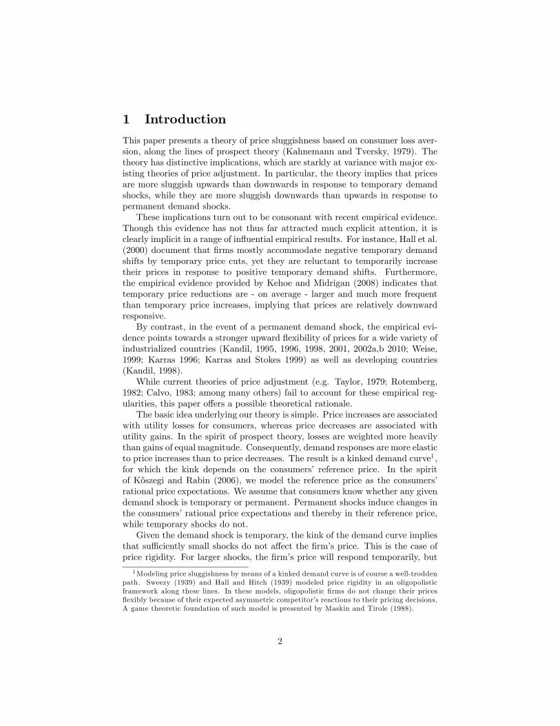
constant, implying that marginal costs are linear in output: MCt(qt) = cqt. Inthe presence of loss aversion (� > ), the downward-sloping demand curve hasa concave kink at the current reference price: bpt = rt. Thus the �rm�s marginalrevenue curve is discontinuous at the kink:

MRt (qt; rt; �) =

�1� 1

�

� qt

r(���)t P �t Yt

!� 1�

; (10)

with � = for the gain domain and � = � for the loss domain, respec-tively. The interval [MRt (bqt; rt; ) ; MRt (bqt; rt; �)], where MRt (bqt; rt; ) <MRt (bqt; rt; �), we call �marginal revenue discontinuity�MRDt(bqt; rt; ; �).

8The positive relationship between reference price and demand has become a common fea-ture in the marketing sciences (e.g., Thaler, 1985; Putler, 1992; Greenleaf, 1995). It manifestsitself, e.g., through the "suggested retail price," by which raising the consumers� referenceprice causes increases in demand (Thaler, 1985). Furthermore, Putler (1992) provides evi-dence that an extensive use of promotional pricing in the late 80�s had lead to an erosion indemand by lowering consumers�reference prices.

9Many authors have shown that consumers�discount rates are generally much higher in theshort run than in the long run (e.g. Loewenstein and Thaler, 1989; Ainslie, 1992; Loewensteinand Prelec, 1992; Laibson, 1996, 1997). Firm behavior is also often found to be short-sightedfor the same reason. The theory of managerial myopia argues that managers often almostexclusively focus on short-term earnings (either because they have to meet certain goals orbecause their career advancement and compensation structure depends on the �rm�s currentperformance), even if this has adverse long-run e¤ects (Jacobson and Aaker, 1993; Grahamet al., 2005; Mizik and Jacobson, 2007; Mizik, 2010). For a review of the early literature referto Grant et al. (1996).

9

pric

e

quantityqss∗

rss= pss∗

marginal revenue curve (gaindomain)

demand curve (gaindomain)

marginal cost curve

marginal revenue curve (lossdomain)

demand curve (loss domain)

MR ss(qss∗ ,  rss, γ )

MRss(qss∗ ,  rss, δ )

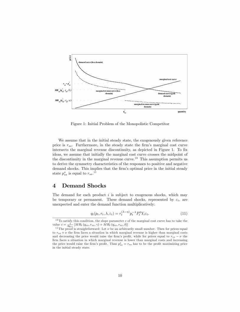
Figure 1: Initial Problem of the Monopolistic Competitor

We assume that in the initial steady state, the exogenously given referenceprice is rss. Furthermore, in the steady state the �rm�s marginal cost curveintersects the marginal revenue discontinuity, as depicted in Figure 1. To �xideas, we assume that initially the marginal cost curve crosses the midpoint ofthe discontinuity in the marginal revenue curve.10 This assumption permits usto derive the symmetry characteristics of the responses to positive and negativedemand shocks. This implies that the �rm�s optimal price in the initial steadystate p�ss is equal to rss.

11

4 Demand Shocks

The demand for each product i is subject to exogenous shocks, which maybe temporary or permanent. These demand shocks, represented by "t, areunexpected and enter the demand function multiplicatively:

qt(pt; rt; �; "t) = r(���)t p��t P �t Yt"t: (11)

10To satisfy this condition, the slope parameter c of the marginal cost curve has to take thevalue c = 1

2qss[MRt (qss; rss; ) +MRt (qss; rss; �)]

11The proof is straightforward: Let � be an arbitrarily small number. Then for prices equalto rss + � the �rm faces a situation in which marginal revenue is higher than marginal costsand decreasing the price would raise the �rm�s pro�t, while for prices equal to rss � � the�rm faces a situation in which marginal revenue is lower than marginal costs and increasingthe price would raise the �rm�s pro�t. Thus p�ss = rss has to be the pro�t maximizing pricein the initial steady state.

10

The corresponding marginal revenue functions of the �rm are

MRt (qt; rt; �; "t) =

�1� 1

�

� qt

r(���)t P �t Yt"t

!� 1�

: (12)

We consider the e¤ects of a demand shock that hits the economy in periodt = 0. The demand shock shifts the marginal revenue curve, along with themarginal revenue discontinuityMRDt (bqt; rt; ; �; "t). We de�ne a "small" shockas one that leaves the marginal cost curve passing through the marginal revenuediscontinuity, and a "large" shock as one that shifts the marginal revenue curvesu¢ ciently so that the marginal cost curve no longer passes through the marginalrevenue discontinuity.The maximum size of a small shock for the demand function (11) is

"t (�) =

�1� 1

�

�r1+�t

cP �t Yt; (13)

i.e. "t (�) is the shock size for which the marginal cost curve lies exactly on theboundaries of the shifted marginal revenue discontinuityMRDt (bqt; rt; ; �; "t (�)).12In the analysis that follows, we will distinguish both between small and largedemand shocks and between temporary and permanent demand shocks.

4.1 Temporary Demand Shocks

For a temporary (one-period) demand shock, the consumers�reference price isnot a¤ected (since information reaches them with a one-period lag and theyhave rational expectations). Thus the �rm�s price response to the shock is thesame as that of a myopic �rm (which maximizes its current period pro�t).

Proposition 1: In response to a small temporary shock, prices remain rigid.

As noted, for a su¢ ciently small demand shock "s0 � "0 (�) the marginalcost curve still intersects the marginal revenue discontinuity, i.e. MC0 ( bq0) 2MRD0 ( bq0; rss; ; �; "s0). Therefore, the prevailing steady state price remains the�rm�s pro�t-maximizing price,13 i.e. p�0 = p

�ss, and we have complete price rigid-

ity. By contrast, the pro�t-maximizing quantity changes to q�0 = r��ss P�0 Y0"

s0,

thus the change of quantity is given by

�q�0 =q�0q�ss

="s0"ss

= "s0 6= 1: (14)

This holds true irrespective of the sign of the small temporary demand shock.

12For " (�), the marginal cost curve intersects the marginal revenue gap on the upper bound,whereas for " ( ) it intersects it on the lower bound.13Compare the proof from Section 3.2.

11

Proposition 2: In response to a large temporary shock, prices are more slug-gish upwards than downwards.

For a large shock, i.e. "l0 > "0 (�), the marginal cost curve intersects themarginal revenue curve outside the discontinuity of the latter. Consequentlyboth, a price and a quantity reaction are induced. The new pro�t-maximizingprice of the �rm is

p�0 =

r(���)ss P �0 Y0"

l0

q�0

! 1�

; (15)

while its corresponding pro�t-maximizing quantity is

q�0 =

�1

c

�1� 1

�

�� ��+1 �

r(���)ss P �0 Y0"l0

� 1�+1

; (16)

where � = � for positive and � = for negative shocks, respectively.In comparison to the standard �rm the price reaction of the �rm facing

loss-averse consumers in response to a large temporary demand shock is alwayssmaller, whereas the quantity reaction is always larger. Additionally, prices andquantities are less responsive to positive than to negative shocks. The intuitionis obvious once we decompose the demand shock into the maximum small shockand the remainder:

"l0 = "0 (�) + "rem0 : (17)

From our theoretical analysis above, the maximum small shock "0 (�) has noprice e¤ects, but feeds one-to-one into demand. This holds true irrespective ofthe sign of the shock. By contrast, the remaining shock "rem0 has asymmetrice¤ects. Let q0 be the quantity corresponding to "0 (�). Then the change inquantity in response to "rem0 is given by

�qrem0 =q�0q0=

�"rem0"0 (�)

� 1�+1

: (18)

As can be seen from equation 18, the change of quantity in response to "rem0depends negatively on �, the price elasticity of demand. Since by de�nition� > , the quantity reaction of the �rm facing loss-averse consumers is smallerin response to large positive temporary demand shocks than to large negativeones. This however implies that prices are also less responsive to positive thanto negative large temporary demand shocks, because the former move the �rmalong the relatively �at portion of the demand curve, whereas the latter moveit along the relatively steep portion of the demand curve. This asymmetricsluggishness in the reaction to positive and negative large temporary demandshocks is a distinct feature of consumer loss aversion and stands in obviouscontrast to the standard textbook case of monopoly pricing.

12

Parameter Symbol ValueDiscount rate � 0:99Elasticity of substitution � 5

implying substitutability � 0:8Price elasticity (gain domain) 6Price elasticity (loss domain) � 12Loss aversion � 2Exogenous nominal income Y 1Exogenous price index Pt 1

Table 1: Base calibration

4.2 Permanent Demand Shocks

Now consider a permanent, demand shock that occurs in period t = 0. Whereasthe �rm is assumed to change its price immediately in response to this shock,consumers update their reference price in the following period t = 1, i.e. r1 =E0[p1]. Consequently, for price increases (decreases) the demand curve shiftsoutwards (inwards) and the kink moves to

( bp1; bq1) = (r1; (P1=r1)� Y1"1) : (19)

An outward shift of the demand curve (initiated by an upward adjustment inthe reference price) increases the �rm�s long-run pro�ts, whereas an inwardshift (initiated by a downward adjustment of the reference price) lowers them.We term this phenomenon the �reference-price updating e¤ect.�The �rm cananticipate this. Thus, it may have an incentive to set its price above the levelthat maximizes its pro�ts in the shock period p00 > p�0, therewith exploiting(dampening) the outward (inward) shift of the demand curve resulting from theupward (downward) adjustment of the consumers�reference price for positive(negative) permanent shocks.14 Whether this occurs depends on whether the�rm�s gain from a price rise relative to p�0 in terms of future pro�ts (�1(r1 =p00) > �1(r1 = p�0), due to the relative rise in the reference price) exceeds the�rm�s loss in terms of present pro�ts (�0(p00) < �0(p

�0), since the price p

00 is not

appropriate for maximizing current pro�t).To analyze which e¤ect dominates, we calibrate the model and solve it nu-

merically.

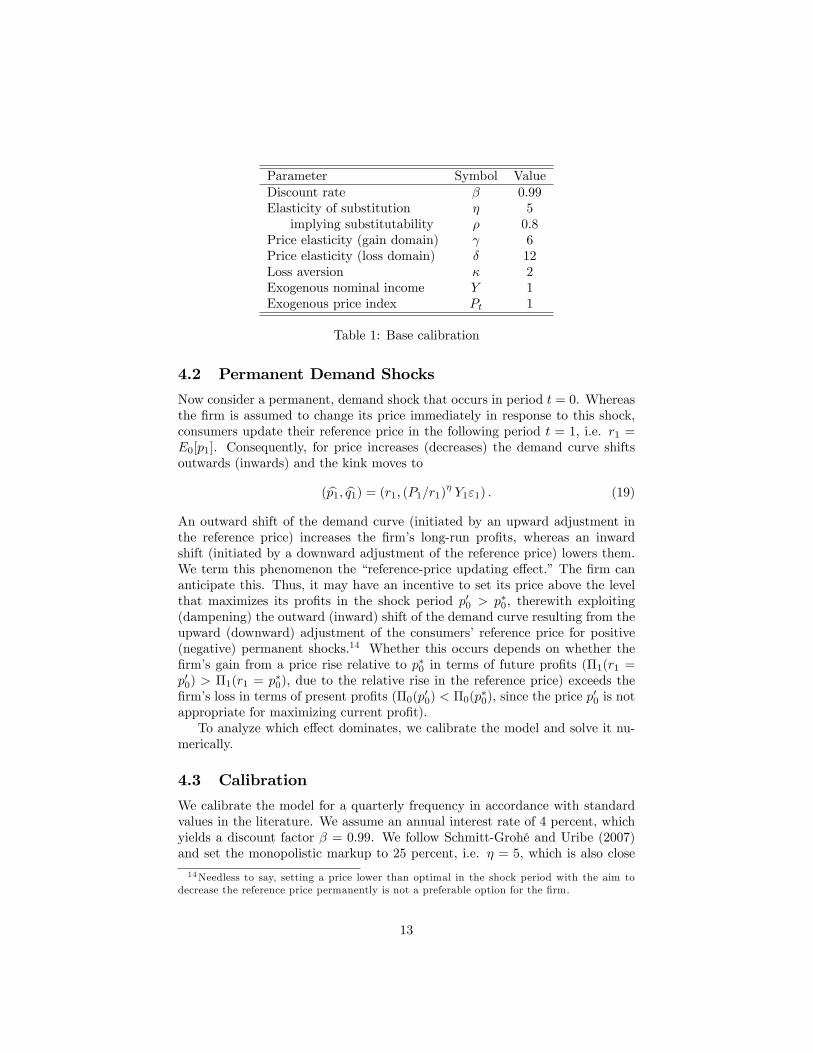
4.3 Calibration

We calibrate the model for a quarterly frequency in accordance with standardvalues in the literature. We assume an annual interest rate of 4 percent, whichyields a discount factor � = 0:99. We follow Schmitt-Grohé and Uribe (2007)and set the monopolistic markup to 25 percent, i.e. � = 5, which is also close

14Needless to say, setting a price lower than optimal in the shock period with the aim todecrease the reference price permanently is not a preferable option for the �rm.

13

temporary shock permanent shock�";p �";q �";p �";q

"s0 = 1:01 0 1 0.0100 0.8789"s0 = 1:03 0 1 0.0667 0.1866"l0 = 1:05 0.0035 0.9560 0.0755 0.0717"l0 = 1:07 0.0232 0.7046 0.0790 0.0216

Table 2: Shock elasticities of price and output in t = 0 to positive permanentdemand shocks, "0 ( ) = 1:0476

temporary shock permanent shock�";p �";q �";p �";q

"s0 = 0:99 0 1 0 1"s0 = 0:97 0 1 0 1"l0 = 0:95 0.0072 0.9592 0.0012 0.9934"l0 = 0:93 0.0484 0.7264 0.0013 0.9927

Table 3: Shock elasticities of price and output in t = 0 to negative permanentdemand shocks; "0 (�) = 0:9524

to the value supported by Erceg et al. (2000) and which implies that goods areonly little substitutable, i.e. � = 0:8. Since we impose � � �, we set = 6 in ourbase calibration. Loss aversion is measured by the relative slopes of the demandcurves in the gain and loss domain, i.e. � = �

. The empirical literature onloss aversion in prices �nds that losses induce demand reactions approximatelytwice as large as gains (Tversky and Kahnemann, 1991; Putler, 1992; Hardie etal., 1993; Gri¢ n and Schulman, 2005; Adeyemi and Hunt, 2007). Therefore, weset � = 2. The exogenous nominal income Y and price index Pt are normalizedto unity.15 The base calibration is summarized in Table 1.

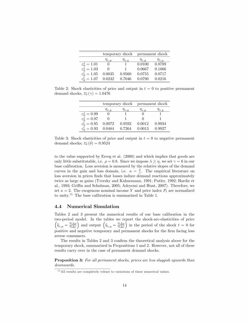
4.4 Numerical Simulation

Tables 2 and 3 present the numerical results of our base calibration in thetwo-period model. In the tables we report the shock-arc-elasticities of price�e�";p = %�p

%�"

�and output

�e�";q = %�q%�"

�in the period of the shock t = 0 for

positive and negative temporary and permanent shocks for the �rm facing lossaverse consumers.The results in Tables 2 and 3 con�rm the theoretical analysis above for the

temporary shock, summarized in Propositions 1 and 2. However, not all of theseresults carry over in the case of permanent demand shocks.

Proposition 3: For all permanent shocks, prices are less sluggish upwards thandownwards.15All results are completely robust to variations of these numerical values.

14

In line with the theoretical analysis above, our numerical results in table2 and 3 indicate that in the case of a permanent shock the �rm exploits the"reference-price updating e¤ect" and generally sets a price that is higher thanthe price it would optimally set in response to a temporary shock, i.e. p00 > p

�0.

For positive permanent demand shocks this implies that the pricing reaction ofthe �rm is always stronger than for positive temporary demand shocks for both,small16 and large shocks17 . By contrast, for negative permanent demand shocks�rms either do not adjust their prices at all for su¢ ciently small shocks or to aconsiderably lower extent than for negative temporary shocks.As a consequence, price sluggishness is considerably less pronounced for pos-

itive than for negative permanent demand shocks. The asymmetry of the pricereaction to positive and negative shocks therefore reverses, when moving fromtemporary to permanent shocks. While this result may seem surprising at �rstglance, it is straightforward intuitively: As noted, for temporary shocks, con-sumers abstract from updating their reference price. Therefore, the �rm doesnot risk to su¤er from a downward adjustment of the consumers�reference price,when encountering a temporary drop in demand with a price reduction. On theother hand, for positive temporary shocks, the �rm cannot generate permanentincreases in demand due to upward-adjustments of the reference price. Sinceconsumers react more sensitive to price increases relative to price decreases, theprice and quantity reactions are smaller for positive temporary shocks comparedto negative ones. By contrast, for permanent demand shocks, the �rm exploitsthe positive "reference-price updating e¤ect" which follows from price increasesin response to positive shocks, whereas it tries to avoid the negative "reference-price updating e¤ect" which follows from price decrease in response to negativeshocks.18

5 Conclusion

In contrast to the standard time-dependent and state-dependent models of pricesluggishness, our theory of price adjustment is able to account for asymmetricprice and quantity responses to positive and negative temporary and permanentshocks of equal magnitude. In contrast to the New Keynesian literature, ourexplanation of price adjustment is thoroughly microfounded, without recourseto ad hoc assumptions concerning the frequency of price changes or physical

16Of course, one can �nd a range of shocks, which are small enough to induce full pricerigidity for permanent positive shocks. Due to the reference-price updating e¤ect, this thresh-old is, however, very small. Given the base calibration, the threshold value for a su¢ cientlysmall positive shock is "0 (�) = 1:0087.17Our numerical analysis indicates, however, that the positive reference-price updating e¤ect

is never strong enough to invalidate the general result that the pricing reaction of the �rmfacing loss averse consumers is more sluggish compared to the standard �rm.18Since the �rm avoids price reductions, which lead to downward-adjustments in the ref-

erence price, but conducts price reductions, which do not in�uence the reference price, lossaversion o¤ers a simple rationale for the �rm�s practice of �sales�.

15

costs of price adjustments.There are many avenues of future research. Consideration of heterogeneous

�rms and multi-product �rms will enable this model to generate asynchronousprice changes, as well as the simultaneous occurrence of large and small pricechanges, and heterogeneous frequency of price changes across products. Extend-ing the model to a stochastic environment will generate testable implicationsconcerning the variability of individual prices. Furthermore, our model needsto be incorporated into a general equilibrium setting to validate the predictionsof our theory.

6 References

Abeler, J., A. Falk, L. Goette, and D. Hu¤man (2011). Reference points ande¤ort provision. American Economic Review 101(2), 470-492.

Adeyemi, O.I. and L.C. Hunt (2007). Modelling OECD industrial energy de-mand: Asymmetric price responses and energy-saving technical change. EnergyEconomics 29(4), 693-709.

Ainslie, G.W. (1992). Picoeconomics. Cambridge: Cambridge University Press.

Alvarez, L.J. and I. Hernando (2005). The price setting behavior of Spanish�rms: Evidence from survey data. Working Paper Series 0538, European Cen-tral Bank.

Amirault, D., C. Kwan, and G. Wilkinson (2005). Survey of price-setting behav-iour of Canadian companies. Bank of Canada Review - Winter 2004-2005, 29-40.

Apel, M., R. Friberg, and K. Hallsten (2005). Microfoundations of macroeco-nomic price adjustment: Survey evidence from Swedish �rms. Journal of Money,Credit and Banking 37(2), 313-338.

Aucremanne, L. and M. Druant (2005). Price-setting behaviour in Belgium:What can be learned from an ad hoc survey? Working Paper Series 0448, Eu-ropean Central Bank.

Ball, L. and N.G. Mankiw (1994). Asymmetric price adjustment and economic�uctuations. Economic Journal 104(423), 247-261.

Bidwell, M.O., B.R. Wang, and J.D. Zona (1995). An analysis of asymmetricdemand response to price changes: The case of local telephone calls. Journal ofRegulatory Economics 8(3), 285-298.

Blinder, A., E.R.D. Canetti, D.E. Lebow, and J.B. Rudd (1998). Asking aboutprices: A new approach to understanding price stickiness. New York: Russel

16

Sage Foundation.

Caballero, R.J. and E.M.R.A. Engel (1993). Heterogeneity and output �uctu-ations in a dynamic menu-cost economy. Review of Economic Studies 60(1),95-119.

Caballero, R.J. and E.M.R.A. Engel (2007). Price stickiness in Ss models: Newinterpretations of old results. Journal of Monetary Economics 54(Supplement),100-121.

Calvo, G.A. (1983). Staggered prices in a utility-maximizing framework. Jour-nal of Monetary Economics 12(3), 383-398.

Caplin, A.S. and D.F. Spulber (1987). Menu costs and the neutrality of money.The Quarterly Journal of Economics 102(4), 703-725.

Card, D. and G.B. Dahl (2011). Family violence and football: The e¤ect ofunexpected emotional cues on violent behavior. The Quarterly Journal of Eco-nomics 126(1), 103-143.

Cover, J.P. (1992). Asymmetric e¤ects of positive and negative money-supplyshocks. The Quarterly Journal of Economics 107(4), 1261-1282.

Crawford, V.P. and J. Meng (2011). New York City cab drivers�labor supplyrevisited: Reference-dependent preferences with rational-expectations targetsfor hours and income. American Economic Review 101(5), 1912-1932.

DeLong, J.B. and L.H. Summers (1988). How does macroeconomic policy a¤ectoutput? Brookings Papers on Economic Activity 19(2), 433-494.

Dixit, A.K. and J.E. Stiglitz (1977). Monopolistic competition and optimumproduct diversity. American Economic Review 67(3), 297-308.

Dossche, M., F. Heylen, and D. Van den Poel (2010). The kinked demand curveand price rigidity: Evidence from scanner data. Scandinavian Journal of Eco-nomics 112(4), 723-752.

Dotsey, M., R.G. King, and A.L. Wolman (2009). In�ation and real activitywith �rm level productivity shocks. 2009 Meeting Papers 367, Society for Eco-nomic Dynamics.

Eichenbaum, M., N. Jaimovich, and S. Rebelo (2011). Reference prices, costs,and nominal rigidities. American Economic Review 101(1), 234-262.

Elmaghraby, W. and P. Keskinocak (2003). Dynamic pricing in the presenceof inventory considerations: Research overview, current practices, and future

17

directions. Management Science 49(10), 1287-1309.

Erceg, C.J., D.W. Henderson, and A.T. Levin (2000). Optimal monetary policywith staggered wage and price contracts. Journal of Monetary Economics 46(2),281-313.

Fabiani, S., M. Druant, I. Hernando, C. Kwapil, B. Landau, C. Loupias, F.Martins, T. Mathä, R. Sabbatini, H. Stahl, and A. Stockman (2006). What�rm�s surveys tell us about price-setting behavior in the Euro area. Interna-tional Journal of Central Banking 2(3), 1-45.

Fabiani, S., A. Gattulli, and R. Sabbatini (2004). The pricing behaviour ofItalian �rms: New survey evidence on price stickiness. Working Paper Series0333, European Central Bank.

Genesove, D. and C. Mayer (2001). Loss aversion and seller behavior: Evidencefrom the housing market. The Quarterly Journal of Economics 116(4), 1233-1260.

Gertler, M. and J. Leahy (2008). A Phillips curve with an Ss foundation. Jour-nal of Political Economy 116(3), 533-572.

Golosov, M. and R.E. Lucas Jr. (2007). Menu costs and Phillips curves. Jour-nal of Political Economy 115(2), 171-199.

Graham, J.R., C.R. Harvey, and S. Rajgopal (2005). The economic implicationsof corporate �nancial reporting. Journal of Accounting and Economics 40(1-3),3-73.

Grant, S., S. King, and B. Polak (1996). Information externalities, share-pricebased incentives and managerial behaviour. Journal of Economic Surveys 10(1),1-21.

Greenleaf, E.A. (1995). The impact of reference-price e¤ects on the pro�tabilityof price promotions. Marketing Science 14(1), 82-104.

Greenslade, J.V. and M. Parker (2012). New insights into price-setting behav-iour in the UK: Introduction and survey results. Economic Journal 122(558),F1-F15.

Gri¢ n, J.M. and C.T. Schulman (2005). Price asymmetry in energy demandmodels: A proxy for energy-saving technical change? The Energy Journal 0(2),1-22.

Hall, R. and C. Hitch (1939). Price theory and business behaviour. OxfordEconomic Papers 2(1), 12-45.

18

Hall, S., M. Walsh, and A. Yates (2000). Are UK companies� prices sticky?Oxford Economic Papers 52(3), 425-446.

Hardie, B.G.S., E.J. Johnson, and P.S. Fader (1993). Modeling loss aversion andreference dependence e¤ects on brand choice. Marketing Science 12(4), 378-394.

Heidhues, P. and B. K½oszegi (2005). The impact of consumer loss aversion onpricing. CEPR Discussion Papers No. 4849, Centre for Economic Policy Re-search.

Heidhues, P. and B. K½oszegi (2008). Competition and price variation when con-sumers are loss averse. American Economic Review 98(4), 1245-1268.

Heidhues, P. and B. K½oszegi (forthcoming). Regular prices and sales. Theoret-ical Economics, forthcoming.

Hoeberichts, M. and A. Stokman (2010). Price setting behaviour in the Nether-lands: Results of a survey. Managerial and Decision Economics 31(2-3), 135-149.

Jacobson, R. and D. Aaker (1993). Myopic management behavior with e¢ cient,but imperfect, �nancial markets : A comparison of information asymmetries inthe U.S. and Japan," Journal of Accounting and Economics 16(4), 383-405.

Kahneman, D. und A. Tversky (1979). Prospect theory: An analysis of decisionunder risk. Econometrica 47(2), 263-291.

Kalwani, M.U., C.K. Yim, H.J. Rinne, and Y. Sugita (1990). A price expec-tations model of customer brand choice. Journal of Marketing Research 27(3),251-262.

Kalyanaram, G. and L.D.C. Little (1994). An empirical analysis of latitude ofprice acceptance in consumer package goods. Journal of Consumer Research21(3), 408-418.

Kandil, M. (1995). Asymmetric Nominal Flexibility and Economic Fluctua-tions. Southern Economic Journal 61(3), 674-695.

Kandil, M. (1996). Sticky wage or sticky price? Analysis of the cyclical behaviorof the real wage. Southern Economic Journal 63(2), 440-459.

Kandil, M. (1998). Supply-side asymmetry and the non-neutrality of demand�uctuations. Journal of Macroeconomics 20(4), 785-809.

Kandil, M. (1999). The asymmetric stabilizing e¤ects of price �exibility: His-torical evidence and implications. Applied Economics 31(7), 825-839.

19

Kandil, M. (2001). Asymmetry in the e¤ects of US government spending shocks:Evidence and implications. The Quarterly Review of Economics and Finance41(2), 137-165.

Kandil, M. (2002a). Asymmetry in the e¤ects of monetary and governmentspending shocks: Contrasting evidence and implications. Economic Inquiry40(2), 288-313.

Kandil, M. (2002b). Asymmetry in economic �uctuations in the US economy:The pre-war and the 1946�1991 periods compared. International EconomicJournal 16(1), 21-42.

Kandil, M. (2006). Asymmetric e¤ects of aggregate demand shocks across U.S.industries: Evidence and implications. Eastern Economic Journal 32(2), 259-283.

Kandil, M. (2010). The asymmetric e¤ects of demand shocks: international ev-idence on determinants and implications. Applied Economics 42(17), 2127-2145.

Karras, G. (1996). Why are the e¤ects of money-supply shocks asymmetric?Convex aggregate supply or �pushing on a string�? Journal of Macroeconomics18(4), 605-619.

Karras, G. and H.H. Stokes (1999). On the asymmetric e¤ects of money-supplyshocks: International evidence from a panel of OECD countries. Applied Eco-nomics 31(2), 227-235.

Kehoe, P.J. and V. Midrigan (2008). Temporary price changes and the reale¤ects of monetary policy. NBER Working Papers 14392, National Bureau ofEconomic Research, Inc.

Knetsch, J.L. and W.-K. Wong (2009). The endowment e¤ect and the referencestate: Evidence and manipulations. Journal of Economic Behavior & Organi-zation 71(2), 407-413.

K½oszegi, B. and M. Rabin (2006). A model of reference-dependent preferences.The Quarterly Journal of Economics 121(4), 1133-1165.

K½oszegi, B. and M. Rabin (2007). Reference-dependent risk attitudes. Ameri-can Economic Review 97(4), 1047-1073.

K½oszegi, B. and M. Rabin (2009). Reference-dependent consumption plans.American Economic Review 99(3), 909-936.

20

Krishnamurthi, L., T. Mazumdar, and S.P. Raj (1992). Asymmetric responseto price in consumer brand choice and purchase quantity decisions. Journal ofConsumer Research 19(3), 387-400.

Kwapil, C., J. Scharler, and J. Baumgartner (2010). How are prices adjustedin response to shocks? Survey evidence from Austrian �rms. Managerial andDecision Economics 31(2-3), 151-160.

Laibson, D. (1996). Hyperbolic discount functions, undersaving, and savingspolicy. NBER Working Papers 5635, National Bureau of Economic Research,Inc.

Laibson, D. (1997). Golden eggs and hyperbolic discounting. The QuarterlyJournal of Economics 112(2), 443-77.

Langbraaten, N., E.W. Nordbø, and F. Wulfsberg (2008). Price-setting behav-iour of Norwegian �rms - Results of a survey. Norges Bank Economic Bulletin79(2), 13-34.

Loewenstein, G. and D. Prelec (1992). Anomalies in intertemporal choice: Evi-dence and an interpretation. The Quarterly Journal of Economics 107(2), 573-97.

Loewenstein, G. and R.H. Thaler (1989). Anomalies: Intertemporal choice. TheJournal of Economic Perspectives 3(4), 181-193.

Loupias, C. and R. Ricart (2004). Price setting in France: New evidence fromsurvey data. Working Paper Series 0423, European Central Bank.

Lünnemann, P. and T.Y. Mathä (2006). New survey evidence on the pricingbehaviour of Luxembourg �rms. Working Paper Series 0617, European CentralBank.

Martins, F. (2010). Price stickiness in Portugal evidence from survey data.Managerial and Decision Economics 31(2-3), 123-134.

Marzilli Ericson, K.M. and A. Fuster (2011). Expectations as endowments:Evidence on reference-dependent preferences from exchange and valuation ex-periments. The Quarterly Journal of Economics 126(4), 1879-1907.

Mas, A. (2006). Pay, reference pay and police performance. The QuarterlyJournal of Economics 121(3), 783-821.

Maskin, E. and J. Tirole (1988). A theory of dynamic oligopoly, II: Price com-petition, kinked demand curves, and Edgeworth cycles. Econometrica 56(3),

21

571-99.

Mayhew, G.E and R.S. Winer (1992). An empirical analysis of internal andexternal reference prices using scanner data. Journal of Consumer Research19(1), 62-70.

McDonald, I.M. and H. Sibly (2001). How monetary policy can have permanentreal e¤ects with only temporary nominal rigidity. Scottish Journal of PoliticalEconomy 48(5), 532-46.

McDonald, I.M. and H. Sibly (2005). The diamond of macroeconomic equilibriaand non-in�ationary expansion. Metroeconomica 56(3), 393-409.

Mehrara, M. and A.R. Karsalari (2011). Asymmetric e¤ects of monetary shockson economic activities: The case of Iran. Journal of Money, Investment andBanking 20, 62-74.

Midrigan, V. (2011). Menu costs, multiproduct �rms, and aggregate �uctua-tions. Econometrica 79(4), 1139-1180.

Mizik, N. (2010). The theory and practice of myopic management. Journal ofMarketing Research 47(4), 594-611.

Mizik, N. and R. Jacobson (2007). Myopic marketing management: Evidenceof the phenomenon and its long-term performance consequences in the SEOcontext. Marketing Science 26(3), 361-379.

Morgan, A. (2008). Loss aversion and a kinked demand curve: Evidence fromcontingent behaviour analysis of seafood consumers. Applied Economics Letters15(8), 625-628.

Morgan, D.P. (1993). Asymmetric e¤ects of monetary policy. Federal ReserveBank of Kansas City Economic Review QII, 21-33.

Nasiry, N. and I. Popescu (2011). Dynamic pricing with loss-averse consumersand peak-end anchoring. Operations Research 59(6), 1361-1368.

Nicolau, J.L. (2008). Testing reference dependence, loss aversion and diminish-ing sensitivity in Spanish tourism. Investigationes Económicas 32(2), 231-255.

Nicolitsas, D. (2013). Price setting practices in Greece: Evidence from a small-scale �rm-level survey. Working Papers 156, Bank of Greece.

Ólafsson, T.T., Á. Pétursdóttir, and K.Á. Vignisdóttir (2011). Price setting inturbulent times: Survey evidence from Icelandic �rms. Working Paper No. 54,

22

Central Bank of Iceland.

Okun, A.M. (1981). Prices and quantities: A macroeconomic analysis. Brook-ings Institution, Washington, DC.

Pope, D.G. and M.E. Schweitzer (2011). Is Tiger Woods loss averse? Persistentbias in the face of experience, competition, and high stakes. American EconomicReview 101(1), 129-157.

Popescu, I. and Y. Wu (2007). Dynamic pricing strategies with reference e¤ects.Operations Research 55(3), 413-429.

Post, T., M.J. van den Assem, G. Baltussen, and R.H. Thaler (2008). Deal orno deal? Decision making under risk in a large-payo¤ game show. AmericanEconomic Review 98(1), 38-71.

Putler, D.S. (1992). Incorporating reference price e¤ects into a theory of con-sumer choice. Marketing Science 11(3), 287-309.

Raman, K. and F.M. Bass (2002). A general test of reference price theory inthe presence of threshold e¤ects. Tijdschrift voor Economie en ManagerrientXLVII(2), 205-226.

Ravn, M.O. and M. Sola (2004). Asymmetric e¤ects of monetary policy in theUnited States. Federal Reserve Bank of St. Louis Review 86(5), 41-60.

Rosenkranz, S. (2003). The manufacturer�s suggested retail price. CEPR Dis-cussion Papers 3954, C.E.P.R. Discussion Papers.

Rosenkranz, S. and P.W. Schmitz (2007). Reserve prices in auctions as referencepoints. Economic Journal 117(520), 637-653.

Rotemberg, J.J. (1982). Monopolistic price adjustment and aggregate output.Review of Economic Studies 49(4), 517-531.

Rotemberg, J.J. (2005). Customer anger at price increases, changes in thefrequency of price adjustment and monetary policy. Journal of Monetary Eco-nomics 52(4), 829-852.

Rotemberg, J.J. (2010). Altruistic dynamic pricing with customer regret. Scan-dinavian Journal of Economics 112(4), 646-672.

Ryan, D.L. and A. Plourde (2007). A systems approach to modelling asym-metric demand responses to energy price changes. In: W. A. Barnett and A.Serletis (eds.), International Symposia in Economic Theory and Econometrics,

23

Volume 18, pp. 183-224.

Sahinöz, S. and B. Saraço¼glu (2008). Price-setting behavior In Turkish indus-tries: Evidence from survey data. The Developing Economies 46(4), 363-385.

Schmitt-Grohé, S. and M. Uribe (2007). Optimal simple and implementablemonetary and �scal rules. Journal of Monetary Economics 54(6), 1702-1725.

Sheshinski, E. and Y. Weiss (1977). In�ation and costs of price adjustment.Review of Economic Studies 44(2), 287-303.

Sibly, H. (1996). Consumer disenchantment, loss aversion and price rigidity.Papers 1996-12, Tasmania - Department of Economics.

Sibly, H. (2002). Loss averse customers and price in�exibility. Journal of Eco-nomic Psychology 23(4), 521-538.

Sibly, H. (2007). Loss aversion, price and quality. The Journal of Socio-Economics 36(5), 771-788.

Spiegler, R. (2012). Monopoly pricing when consumers are antagonized by unex-pected price increases: A �cover version�of the Heidhues-K½oszegi-Rabin model.Economic Theory 51(3), 695-711.

Stahl, H. (2005). Price setting in German manufacturing: New evidence fromnew survey data. Working Paper Series 0561, European Central Bank.

Sweezy, P. (1939). Demand under conditions of oligopoly. The Journal of Po-litical Economy 47(4), 568-573.

Tan, S.-H., M.-S. Habibullah, and A. Mohamed (2010). Asymmetric e¤ects ofmonetary policy in ASEAN-4 economies. International Research Journal of Fi-nance and Economics 44, 30-42.

Taylor, J.B. (1979). Staggered wage setting in a macro model. American Eco-nomic Review 69(2), 108-113.

Thaler, R. (1985). Mental accounting and consumer choice. Marketing Science4(3), 199-214.

Thaler, R. (1991). Quasi rational economics. Russell Sage Foundation, NewYork.

Thoma, M.A. (1994). Subsample instability and asymmetries in money-incomecausality. Journal of Econometrics 64(1-2), 279-306.

24

Tversky, A. and D. Kahneman, D. (1991). Loss aversion in riskless choice: Areference-dependent model. The Quarterly Journal of Economics 106(4), 1039-1061.

Weise, C.L. (1999). The asymmetric e¤ects of monetary policy: A nonlinearvector autoregression approach. Journal of Money, Credit and Banking 31(1),85-108.

Zbaracki, M.J., M. Ritson, D. Levy, S. Dutta, and M. Bergen (2004). Man-agerial and customer costs of price adjustment: Direct evidence from industrialmarkets. The Review of Economics and Statistics 86(2), 514-533.

Zhou, J. (2011). Reference dependence and market competition. Journal ofEconomics & Management Strategy 20(4), 1073-1097.

Appendix

1. Demand Curve of Loss Averse Consumers

The loss averse consumer maximizes her utility function (1) subject to her bud-get constraint (3). The corresponding Lagrangian problem reads:

maxqi;t

L =

"nXi=1

�pi;tri;t

���qi;t

!�# 1�

� '"

nXi=1

pi;tqi;t � PtYt

#; (20)

where ' is the Lagrangian multiplier. The �rst-order condition of the La-grangian function (20) is

@Lt@qi;t

=1

�

"nXi=1

�pi;tri;t

���qi;t

!�# 1��1�

pi;tri;t

����q��1i;t �� 'pi;t = 0: (21)

We collect all terms including demand components on the left hand side

q��1i;t

"nXi=1

�pi;tri;t

���qi;t

!�# 1���

= 'pi;t

�pi;tri;t

���; (22)

and simplify the exponentials

qi;t

"nXi=1

�pi;tri;t

���qi;t

!�#� 1�

=

�'pi;t

�pi;tri;t

���� 1��1

: (23)

We de�ne overall demand according to a Dixit and Stiglitz (1977) aggregate,which reads

qt =

"nXi=1

�pi;tri;t

���qi;t

!�# 1�

: (24)

25

Applying (24) as well as the de�nition of the elasticity of substitution (i.e.� = 1

1�� ), we can simplify (23) to

qi;t = ('pi;t)���pi;tri;t

���(��1)qt: (25)

To determine the Lagrangian multiplier ', we plug (25) into (24)

qt =

24 nXi=1

�pi;tri;t

���('pi;t)

���pi;tri;t

���(��1)qt

! ��1�

35�

��1

; (26)

which after some simple manipulations yields

' =

24 nXi=1

pi;t

,�pi;tri;t

���!1��35 1��1

� P�1t : (27)

We de�ne the inverse of the Lagrangian multiplier ' as the overall price indexPt. Plugging (27) back into (25) yields

qi;t = P�t

�pi;tri;t

���(��1)p��i;t qt: (28)

Applying the budget constraint (3) yields

qi;t = P�t

�pi;tri;t

���(��1)p��i;t Yt: (29)

Finally, we simplify (29) using the de�nition � = �(1 + �)� �, which yields thedemand curve for the di¤erentiated good i

qi;t = r���i;t p��i;t P

�t Yt (30)

Including the shock term, equation (30) reads

qi;t = r���i;t p��i;t P

�t Yt"t: (31)

2. Price and Quantity at the Kink

The kink is given by the particular price at which the two demand curves in-tersect, i.e. qi;t(pi;t; ri;t; ) = qi;t(pi;t; ri;t; �). Given (31) and the de�nition of �from equation (7) it must hold that

r ��i;t p� i;t P�t Yt"t = r

���i;t p

��i;t P

�t Yt"t; (32)

26

which simpli�es tor ��i;t p� i;t = r

���i;t p

��i;t : (33)

Sorting terms yieldsp�� i;t = r���� +�i;t : (34)

From (34) it is obvious that pi;t = ri;t at the kink. Plugging (34) back into (31)gives the quantity at the kink

qi;t = r��i;t P

�t Yt"t: (35)

6.1 3. Demand Curve of Standard Consumers

The standard consumer (i.e. the non-loss averse consumer) maximizes her utilityfunction

Ut (q1;t; :::; qn;t) =

"nXi=1

q�i;t

# 1�

; (36)

subject to her budget constraint (3). The corresponding Lagrangian problemreads:

maxqi;t

L =

"nXi=1

q�i;t

# 1�

� �"

nXi=1

pi;tqi;t � PtYt

#; (37)

where � is the Lagrangian multiplier for the standard textbook problem. The�rst-order condition of the Lagrangian problem (37) is

@Lt@qi;t

=1

�

"nXi=1

q�i;t

# 1��1

q��1i;t �� �pi;t = 0: (38)

We collect all terms including demand components on the left hand side andsimplify the exponentials

qi;t

"nXi=1

q�i;t

#� 1�

= (�pi;t)1

��1 : (39)

We de�ne overall demand for the standard consumer by a Dixit and Stiglitz(1977) aggregate of the form

qt =

"nXi=1

q�i;t

# 1�

: (40)

Applying (40) as well as the de�nition of the elasticity of substitution, we cansimplify (39) to

qi;t = (�pi;t)��qt: (41)

27

To determine the Lagrangian multiplier �, we plug (41) into (40)

qt =

"nXi=1

�(�pi;t)

��qt

� ��1�

# ���1

; (42)

which after some simple manipulations yields

� =

"nXi=1

p1��i;t

# 1��1

� P�1t : (43)

We de�ne the inverse of the Lagrangian multiplier � as the overall price index�Pt for the standard textbook problem. Plugging (43) back into (41) yields

qi;t = P�t p

��i;t qt: (44)

Applying the budget constraint (3) yields the demand curve for the di¤erentiatedgood i for the standard consumer

qi;t = p��i;t P

�t Yt (45)

Including the shock term, equation (45) reads

qi;t = p��i;t P

�t Yt"t: (46)

4. Marginal Revenue Curve

Since all �rms are assumed to be identical, we drop the subscript i for the �rmderivations. Revenue is given by

Rt = pt(qt; rt; �; "t)qt =

qt

r(���)t P �t Yt"t

!� 1�

qt; (47)

or in short

Rt =�r(���)t P �t Yt"t

� 1�

q1� 1

�t : (48)

The �rst-order condition with respect to qt yields the marginal revenue curve

MRt =@Rt@qt

=

�1� 1

�

� qt

r(���)t P �t Yt"t

!� 1�

: (49)

28

5. Critical Shock Size

The critical value for the small shock is given by the particular shock "t (�),for which the marginal cost curve exactly intersects the critical bounds of theshifted marginal revenue discontinuity, i.e.

MCt (q�t )

!=MRt (q

�t ; rt; �; "t (�)) ; (50)

where MCt(qt) =@C(qt)@qt

= cqt, with Ct(qt) = c2q2t . Evaluating the marginal

revenue curve (49) and the marginal cost curve at the post-shock optimumyields

cq�t =

�1� 1

�

� q�t

" (�) r(���)t P �t Yt

!� 1�

: (51)

From the analysis of small shocks we know that the new quantity of the maxi-mum small shock is q�t = "t (�) r

��t P �t Yt. Applying this, we obtain

c"t (�) r��t P �t Yt =

�1� 1

�

� "t (�) r

��t P �t Yt

"t (�) r(���)t P �t Yt

!� 1�

: (52)

Solving for "t (�) yields the critical shock size

"t (�) =

�1� 1

�

�r1+�t

cP �t Yt: (53)

6. Optimal Price and Quantity in Reaction to a LargeShock for the Myopic Firm

The new optimal price lies at the intersection of the marginal cost curve withthe shifted marginal revenue curve, which by de�nition is outside the marginalrevenue discontinuity

MCt (q�t ; "t) =MRt (q

�t ; rt; �; "t) : (54)

Applying the respective functions yields

cq�t =

�1� 1

�

� q�t

r(���)t P �t Yt"t

!� 1�

: (55)

Solving this equation for q, we obtain

q�t =

�1

c

�1� 1

�

�� ��+1 �

r(���)t P �t Yt"t

� 1�+1

: (56)

29

The optimal price can be calculated by plugging q�t into the inverse demandcurve, given by

p�t =

q�t

r(���)t P �t Yt"t

!� 1�

: (57)

30