A Theory of Origami World - Robotics Institute · Key Ideas and Related Works 2.1. ... A THEORY OF...

ARTIFICIAL INTELLIGENCE 279

A Theory of Origami World*

Takeo Kanade Department of Computer Science, Carnegie- Mcllon Universiry, Pittsburgh, PA, U.S.A. and Department of Information Science, Kyoto University, Kyoto, Japan

Recommended by Harry Barrow

ABSTRACT The recovery of three-diniensional configurations o fa scene from its image is one of the most important stcps in coniputer vision. The Origami world is a model for understanding line drawings in terms of surfaces, and for finding their 3- D ConfiRurafions. It assumes rho? surfaces themselves can be stand-alone objects, unlike the conventional rrihcdral world which assunies solid objects. We have established a labeling procedure for this Origami world, which canfind the 3-0 meaning of a given line drawing by assigninK one of the labels, + (convex edge), - (concove edgc), t, and 4 (occluding boundary) to each line. The procedure uses afiltcring procedure not only for junction labels as in the Waltz labeling for the irihedral world, but also .for chccking the consistency of surface orientations. The theory includes the Hufnran-Clouv.c labeliti.q.c fiw the trihedrol solirl-object world as a subset. This paper also receals intcrestirig relationships anrong previous research in polyhedral scene analysis.

1. Introduction

Origami is the Japanese traditional manual art of making various shaped objects (e.g., animals) by folding a sheet of paper. Fig. 1 is a typical example of Origami.

FIG. 1 Origami crane.

This research was sponsored by the Defence Advanced Research Projects Agency (DOD), ARPA Order No. 3597, and monitored by the Air Force Avionics Laboratory under Contract F33615-78-C-ISSI.

Artificial Intelligence 13 (1980). 219-31 1 Copyright 8 1980 by North-Holland Publishing Company

280 T. KANADE

Jt is easy to see that Fig. 1 is an Origami crane. This process of seeing and understanding may be divided into two processes: one is to determine the possible three- dimensional configurations from the picture, and the other is to match them with some known concepts (such as ‘crane’). This paper deals with the first process. Thus the problem is: how do we understand the possible three-dimensional configurations from a collection of lines?

One solution is: first, model a world (I will call it the ‘Origami’ world), where surfaces themselves can be stand-alone objects, rather than the conventional trihedral solid-object world; secondly, establish a procedure which can assign a 3-D meaning to each line. The procedure developed uses a filtering method both for finding consistent combinations of labels and for testing the consistency of surface orientations based on the gradient space representation.

2. Key Ideas and Related Works

2.1. Illustrative examples Figs. 2-4 are a few illustrative examples of simple line drawings for the following discussions in this paper. They usually convey to the viewer the meaning intended by the artist: Fig. 2: a ‘box’ (an open-faced cube); Fig. 3 : a ‘cube’ (a convex right- angled corner); and Fig. 4 : a ‘W-folded paper’.

However, take Fig. 3 for example; other possible configurations, such as those

FIG. 2. A ‘box’ line drawing.

FIG. 3. A ‘cube’ line drawing.

FIG. 4. A ‘W-folded paper’ line drawing.

,

A THEORY OF ORIGAMI WORLD 28 1

(a) 0)

FIG. 5. Other interpretations of Fig. 3: (a) a concave comer, (b) a folded paper ‘roof’ covering another paper.

in Fig. 5 , are imaginable. This paper will demonstrate how basic geometric constraints can be exploited to recover such possible shapes of the object that a given drawing may depict.

2.2. Surface-oriented world vs. solid-object world Those who are familiar with the work of Huffman, Clowes and Waltz [l, 4, 131 might think that the problem of recovering 3-D configurations from line drawings had been solved. In fact, the Huffman-Clowes-Waltz labeling method can identify the cube-like configuration of Fig. 3. The method assumes the trihedral world in which exactly three planes meet at a corner, and assigns to lines the labels which represent their 3-D meaning, such as + (convex edge), - (concave edge), and c or -+ (occluding boundary). Thus, Fig. 3 is given a labeling as shown in Fig. 6,

FIG. 6. Huffrnan-Clowes-Waltz labeling representing a cube-like configuration.

which means that we are looking at a corner made of three convex edges, ;.e., a cube-like configuration. This method has various good features:

( I ) a clear-cut definition of the object world (Le., the trihedral world), which results in using knowledge in a systematic way as well as eliminating vague heuristics,

(2) a compiled knowledge representation in the form of ajunction dictionary, and (3) an efficient labeling procedure by filtering. However, the Huffman-Clowes-Waltz labeling cannot generate interpretations

.. - of Fig. 3 other than a cube, or cannot deal with Fig. 2 and Fig. 4; it would call- them ‘impossible objects’. But those pictures appear to be perfect drawings. The reason for this failure is revealed in the first sentence of [SI :

“Objects bounded by planes were reasonable ones upon which to do initial research in scene analysis . . .”

. .. ,

282 T. KANADE

FIG. 7. ‘Super’ perfect line drawing of a box.

That is, plane surfaces have been attributes of objects. In other words, it has been assumed that solid objects are the basic stand-alone units of the world of Huffman- Clowes-Waltz labeling. Thus the line drawing of a box would need to be ‘super’ perfect, as in Fig. 7. What would be useful is to expand the world to one that includes surfaces as the basic units. The world will be called the ’Origami’ world, but this term is intended only to bring to mind the idea of the surface-oriented world, and does not imply anything about the nature of paper.

Several people have attempted to expand the Huffman-Clowes-Waltz scheme. One attempt is to allow more complex surfaces than planes. Turner [I21 tried to extend the Waltz-type labeling scheme to include curved objects. Huffman [5] proposed to manipulate paper surfaces (that is, developable surfaces: all points on a given line embedded in the surface have the same tangent plane) as of intermediate complexity between completely general surfaces and the plane surfaces.

Another direction of attempt is to understand scenes using more data than simple line drawings. Sanker [IO] extended Huffman-Clowes labeling method to interpret line drawings with hidden lines. Sugihara and Shirai [I 1 J used a junction dictionary to understand scenes for which range data are available.

We can note that the above approaches still assume solid objects bounded by surfaces. In contrast, the present work on the Origami world tries to begin with a more basic unit (Le., surface) in constructing the world. Further discussion on the related work including Guzman [3], Mackworth [SI and Huffman [6] will be found in Section 4 after the theory of the Origami world is presented.

3. The Theory of Origami World The presentation of the theory of the Origami world consists of seven subsections:

(1) Terminology; (2) The enumeration of legal combinations of line labels at junctions; (3) The problem concerning global consistency of surface orientations; (4) The augmented junction dictionary; ( 5 ) A test method for consistency of surface orientations; (6) The actual labeling procedure; (7) Examples of labeling.

3.1. Origami world and terminology The world is assumed to be made of a collection of surfaces. A line drawing is a picture (i.e., a projection to the two-dimensional picture plane) of such a composite

A THEORY OF ORIGAMI WORLD 283

in the scene. We will assume orthographic projection throughout the paper. Surfaces in the Origami world are assumed to be planar; i.e., the orientation is constant throughout a surface. In this respect it is nor the paper-surface (Le., develop able) world investigated by Huffman [5].

The terminology we will use for the Origami world parallels .that for the Waltz labeling theory [13]. An edge is a straight boundary of a plane surface. A uerrex is a point where edges of the surface(s) meet. A line is an orthographic projection of an edge to the picture plane. Ajuncfion is a point in the picture where lines meet. A junction can be the projection of a vertex or the point where an edge is interrupted by an occluding surface. A region is an area in the picture surrounded by lines, and it corresponds to (a visible part of) a surface.

An edge can be classified according to its three-dimensional physical meaning in the scene. We will use the following terms and labels:

edge along which two surfaces meet and form a convexity edge along which two surfaces meet and form a concavity edge along which one surface occludes another

convex + concave - occluding c or +

The direction of the arrow for an occluding boundary is given in such a way that the surface to its right occludes the surface to its left. It might be considered that we should make a distinction between the occluding edges of a sheet and a fold in a sheet by, say, a single arrow (+) and a double arrow (4) as in [4]. The reason that we do not make this distinction will be found in Section 3.4.

A line can therefore be labeled with one of the four labels (+, -, t, and +), according to its physical meaning of the corresponding edge; thus we can say line is convex” to mean that it depicts a convex edge. Therefore, to give line labels to the lines in the drawing is to give a three-dimensional meaning to the drawing. A set of assignments of line labels to the lines in the drawing is called an inrerpretation of the drawing. For example, the labeling shown in Fig. 6 is an interpretation of Fig. 3.

Junctions are classified according to the number of lines meeting at the junctions and their geometrical configurations in the picture. Fig. 8 shows the junction types

ARROW FORK 1 1

X PSI X K AST K

Ro. 8. Junction types. ’

20

284 T. KANADE

called L, ARROW, FORK, T, K, X, PSI, XK, and AST (mostly after Guzman [3] and Waltz [ 13)). ,

I

3.2. ”be enumeration of legal junction labels The physical world imposes constraints on the labels that lines can take at a particular type ofjunction. A combination of line labels for one junction type is referred to as ajuncrion label. The crucial observation which was made by Huffman and Clowes, and which was exploited to a great extent by Waltz, is that not all the combinatorially possible junction labels can appear (are legal) in the picture. For example, for the ARROW junction, only three junction labels out of the 4 x 4 x 4 possible combinations can occur in the trihedral world. Needless to say, unless we assume a certain restriction on the three-dimensional configurations allowable at the vertices, the resultant constraints on junction labels will be too weak to be useful. We need to confine ourselves to a reasonably limited world which corresponds well to the real world images.

The restrictions we adopt in the Origami world are that no more than three surfaces of different orientations meet at a vertex, and that no more than three edges of different orientations are involved at a vertex. We assume that the combination of the three orientations of the surfaces at a vertex is ‘general’ in the sense that they span the three-dimensional space (Le., each orientation has a vector component perpendicular to the other two). Lct us call such vertices up-to-3-surface vertices. This restriction corresponds to the trihedral vertices in the solid-object world. Note, however, that the up-to-3-surface vertices generate a richer world than the world generated by the trihedral vertices, since the former can include 1- and 2-surface vertices; that is, it allows free extending surfaces as stand-alone objects.

Possible junction labels for the upto-3-surface vertices in the Origami world can be enumerated in the following way. The planes of three general orientations intersect and divide each other into 12 partial planes. Thus we can think of 12 quadrant plane surfaces around the vertex point as shown in Fig. 9.

Let us fix our eye position in one of the eight octants separated by the quadrant planes, say, the octant bounded by the quadrants 0,4, and 7. Next, we generate one by one all the possible (4096) combinations by setting each quadrant plane to be

I

! i

FIG. 9. Twelve quadrant plana.

T. KANADE 286

labels thus obtained for L, ARROW, FORK, and T with that of legal trihedral junction labels. It gives an idea of the degree of constraint imposed by the up-to-3- surface Origami world compared with the Huffman-Clowes trihedral-junction world.

3.3. Global consistency of surface orientations

3.3.1. The problem A legal junction label represents a possible configuration of surfaces at an up-to-3- surface vertex. The consistent labeling of a line drawing, so that all the junctions are given legal junction labels, is nothing but a check on the consistency of surface interconnections: this is done by passing information by means of line labels from one junction to another. Waltz filtering [13] on junction labels is known to be a good method for doing this. However, labeling in the Origami world cannot simply rely on the filtering on junction labels. Because of the weaker restrictions at the vertices than the trihedral world, there are a lot of anomalous interpretations [8, 91 in which the labeling is consistent, but the whole configuration is not.

1

(a) (b) (C)

FIG. 12. Interpretation inconsistent with respect to surfaceorientations.

Figure I2 shows one of the simplest examples of such anomaly. The interpretation shown in Fig. 12(b) implies that two surfaces corresponding to the regions R, (ABED) and R, (ACBEFD) are connected at two convex edges AD and BE. All the junctions, A through F, are given legal junction labels. However, it can be easily seen that this configuration is not realizable by the two planar surfaces; one or the other should be bent. Why is this inconsistency not detected by the junction dictionary? The reason is shown in Fig. 12(c). The junction dictionary tells that the line labels given to AD, BE, AB, BC, and CA are consistent because they form legal combinations local/y at each junction A, B, or C. However, no use is made of the fact that the three shaded regions in Fig. 12(c) are actually the same surface and therefore have a unique surface orientation in the scene.

It should be noted that the kinds of anomalies illustrated above, which are caused by relying solely upon the junction dictionary, have also occurred in the Huffman- Clowes-Waltz labeling for the trihedral solid-object world. But because they occurred ‘less frequently,’ they did not show up as a very serious problem. Fig. 13 is

. - - .-. . . . . . . . . . . . __ - . . . ~ . . . . . . .

285 A THEORY OF ORIGAMI WORLD

either occupied or vacant, and check how the vertex formed at the ongin appears when viewed from the eye position fixed as above. Then we can give a label to each line at the junctioH based on its meaning, and obtain a legal junction label. Figs. lO(a) through 10(e) show examples of the vertex configurations and their derived

Fro. 10. Exampla of configurations at vertices: (a) one quadrant plane which generates an L junction, (b) (c) two quadrant planes which generate an ARROW junction, (d) t h m quadrant planes which generate a T junction, (e) four quadrant planes which generate a T junction.

junction labels. Notice that they are legal in the Origami world, but none of them are in the trihedral world. They are typically the results of cutting, folding, and bonding planar surfaces. The number of junction labels thus obtained is: 8 for L, I5 for ARROW, 9 for FORK, 12 for T, 19 for K, 7 for X, 22 for PSI, 41 for XK, and 16 for AST.

FIG. I I . Legal T junction labels not corresponding to vertices (Huffman [4]).

For the junction type T, the four additional junction labels shown in Fig. I 1 are included as legal. They do not correspond to actual vertices, but to the cases in which the junction is caused because the upper half plane is in the front and occludes the edge behind. Table 1 compares the number of legal upto-3-surface junction

TABLE I . Comparison of the size of the Origami junction dictionary with the Huffman-Clowes dictionary

Junction Huffman-Clowes Origami world type dictionary dictionary

L 6 8 ARROW 3 IS FORK 3 9 T 4 16

,

288 T. KANADE

FIG. IS. Constraint on the gradients of regions connected by a coovex (+) or concave (- ) line.

The values of (a, b) represent how the planes are slanting relative to the view line (z axis). For example, the origin OG = (0,O) of G corresponds to those planes (- z = c) perpendicular to the view line. P, = (1,O) corresponds to the planes' (-2 = x + c ) which are slanting horizontally to the right.

One of the useful properties of the gradient space is the following [8]. Consider two planes meeting at an edge and their orthographic picture made of regions R, and R, and a line L, as shown in Fig. 15. Then in the gradient space, the gradients GI and G , of the two planes should be on a gradient-space line which is perpendicular to the picture line L. Moreover, if the edge is convex (+), G, and G, are ordered in the same direction as are the corresponding regions in the picture. If the edge is concave (-), their order is reversed.

3.3.3. Inconsistency of the example Now we are ready to test the example of Fig. 12. Imagine a gradient space and refer to Fig. 16. Let G, be the gradient of the region R,. R, and R2 are connected at the convex line AD in the picture. Thus, the gradient of R2 should be somewhere on the half line Glo, which is perpendicular to AD and extends toward left, because of the property of the gradient space. Suppose it is at G,. Again because R, is connected with R, at a convex line BE, the gradient of R, should be somewhere on the half line G,b as shown. Since we have fixed the gradient of R, at G I , this half line G,b should pass G I , which is impossible wherever we select G, on the half line Gla. When we select G, and G2 at the same location (Le., the two surfaces have the same orientation), the constraint may seem to be satisfied as a special case, but then the convex lines AD and BE would not appear. This means that there is no combination

b

FIG. 16. Trace of gradients of the regions in Fig. 12(b).

,


+

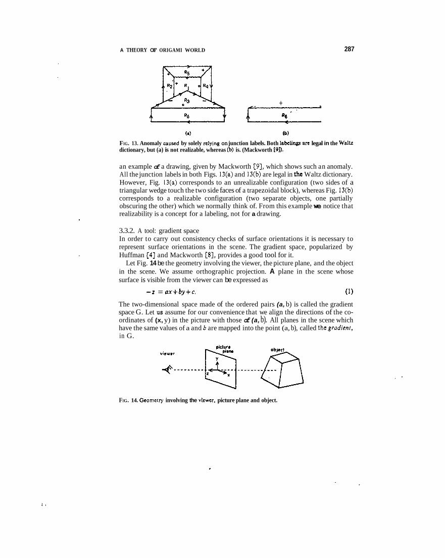
FIG. 13. Anomaly caused by solely relying on junction labels. Both labclings an legal in the W a k dictionary, but (a) is not realizable, whereas (b) is. (Mackworth [9]).

an example of a drawing, given by Mackworth [9], which shows such an anomaly. All the junction labels in both Figs. 13(a) and 13(b) are legal in the Waltz dictionary. However, Fig. 13(a) corresponds to an unrealizable configuration (two sides of a triangular wedge touch the two side faces of a trapezoidal block), whereas Fig. 13(b) corresponds to a realizable configuration (two separate objects, one partially obscuring the other) which we normally think of. From this example we notice that realizability is a concept for a labeling, not for a drawing.

3.3.2. A tool: gradient space In order to carry out consistency checks of surface orientations it is necessary to represent surface orientations in the scene. The gradient space, popularized by Huffman [4] and Mackworth [8], provides a good tool for it.

Let Fig. 14 be the geometry involving the viewer, the picture plane, and the object in the scene. We assume orthographic projection. A plane in the scene whose surface is visible from the viewer can be expressed as

(1) - 2 = ax+by+c .

The two-dimensional space made of the ordered pairs (a, b) is called the gradient space G. Let us assume for our convenience that we align the directions of the coordinates of (x, y) in the picture with those of (a, b). All planes in the scene which have the same values of a and b are mapped into the point (a, b), called thegradient, in G.

FIG. 14. Geometry involving the viewer, picture plane and object.

: r

A THEORY OF ORlGAMl WORLD 289

of gradients for the regions R, and R2 which results in the configuration of Fig. 12(b) ; therefore the configuration is inconsistent.

3.4. The augmented junction dictionary The previous subsection has demonstrated the necessity of and the basic 'tool for more thorough and global consistency checks of surface onqntations than simple labeling. For this purpose we will augment the junction dittionary of the Origami world. Each legal junction label derived in 3.2 implies which surfaces are connected at which edge in order to form that junction label. In the augmented junctiop dictionary, this information is explicitly stored by means of links, which connect a pair of related regions and which include description of the constraints on their gradients.

t

FIG. 17. A link in the augmented junction dictionary.

Two examples of the entries of the augmented dictionary are shown in Figs. 17 and 18. The link in a legal FORKjunction label shown in Fig. 17 represents that the regions R, and R2 are connected at the convex line L, and that their gradients G, and G2 should be on a gradient-space line perpendicular to L with their ordering a5 shown.

I n the example of Fig. 17, the link is redundant, because it only makes explicit

FIG. 18. Link for an occluded intersection line.

290 T. KANADE

the information which the line label (+) attached to L expresses by itself. To this extent it is the same as the predicates used by Clowes [l] to specify the relations between surfaces. However, the links play a substantial role for representing the configuration assuhed at the vertex in the case of junction labels which involve partially occluded regions: such junction labels are peculiar to the Origami world. Take the ARROW junction label shown in Fig. 18(a). As shown in Fig. 18(b), this is typically a result of folding a planar surface along BC; thus S, occludes a part of S1. We can assume, though, that this junction label includes a more general situation in which the intersection line of SI and S2 lies within the angle ABC, rather than just along BC (Fig. 18(c)). We can imagine this configuration as folding a plane twice: first along BC, then along BD. This extended assumption allows interpreting common shapes such as the ‘slide’ shown in Fig. 18(d). For convenience we will describe this situation as follows: the surfaces S, and S, are connected at an ‘occluded intersection’ line L‘ (= BD) which is located within the angle ABC (Fig. I8(e)). Let us use the label @ to indicate the occluded intersection.

If we remove the right hand part of SI which is occluding S,, the rest of SI and S, will form a convex intersection line at L‘. Since L‘ can be anywhere in the angle ABC, as illustrated in Fig. 18(f), if we fix the location of G, in the gradient space, then the gradient G2 should be inside of the fan-shaped area whose origin is at G, ; the area is bounded by the gradient-space lines G,a and G,c which are respectively perpendicular to AB and BC. G2 can be on Glc, but not on G,a, since the occluded intersection line L‘ can coincide with BC, but not with AB. (If it did, the label of AB will change from c to + .) The associated link connecting R, and R2 includes the information described above concerning their gradients. In this way the augmented junction dictionary is constructed by adding appropriate link information to each legal junction label.

C

01 \

: r

FIG. 19. An example o f a vertex which shows that we cannot tell whether an occluding edge is that of a sheet or that of a fold of a sheet. It may change from one to another in the middle o f a line. This can be the case because of the ugto-3-surface assumption. Under the trihedral assumption, an occluding edge is always that of a fold of a sheet; otherwise, there should be a less-than-3- surface vertex.


The example of Fig. I8 also shows one of the reasons that we need not distinguish an occluding edge ofa sheet from that of a fold of a sheet. The line BC can be either one. Moreover, the line BC may change its property from an edge of a sheet to an edge of a fold in the middle of it. As shown in Fig. 19, even when we assume that S , and 3, are folded along BC, who can assure that the lower part of BC is still an edge of a fold?

3.5. A test method for consistency of surface orientations This subsection will present a method which checks the consistency of surface orientations of a given labeling. The method first constructs a labeled graph called Surface Connection Graph using the augmented junction dictionary, and then per- forms a type of filtering operation on it to test the constraints in the gradient space. The method to be presented is closely related to the ideas of the dual graph of Huffman [4], the Face Adjacency Graph of Falk [2], and the POLY program of Mackworth [SI.

3.5.1. Surface connection graph' (SCG) A Surface Conneclion Graph (SCG) is a labeled graph constructed in the following way from agiven interpretation of the line drawing. The nodes of the SCG are regions in the drawing. A pair of nodes are connected by an arc if a junction involving the corresponding pair ofregions has been given ajunction label which has a link between them. To each arc is attached the corresponding link information which has been instantiated by using the directions of the lines at each particular junction. A pair of regions can be connected by multiple arcs if there are several junctions having the links between them.

As examples, the SCG's for Fig. 12(b) and Fig. 13(a) are shown in Fig. 20 and Fig. 21, respectively. The link information attached to the arcs is shown in an abbreviated way by the corresponding line labels. Duplication of links associated with a single line is eliminated in the SCG, such as the links between R, and R, at the vertices A and D in Fig. 20.

The SCG is similar to Falk's Face Adjacency Graph (FAG) in that both are topological graphs with surfaces as nodes to show their interconnections. However, the arcs in the SCG represent more general relationships, such as occluded inter- sections, than simple adjacency of surfaces along convex or concave edges.

-

V R2

FIG. 20. Surface Connection Graph of the interpretation in Fig. 12(b).

292 T. KANADE

FIG. 21. Surface Connection Graph o f the interpretation in Fig. I3(a).

3.5.2. Spanning angles and their computation Let G I and G, denote the gradients of R, and R,, respectively. Suppose the nodes R, and R2 in an SCG are connected by an arc corresponding to a convex intersection line L. Mathematically, the constraint imposed by the arc can be represented as

Here P is a two-dimensional unit vector (IPI = 1) with a direction perpendicular to L, and pointing from R, to R,. The k is a positive scalar constant. If the kind of intersection is concave (-), then the constraint between G I and G2 is also represented by the form (2), but in this case P points from R2 to R1, as shown in Fig. 15. If the intersection line is an occluded intersection (@), the constraint between G, and G, is represented as

GZ-GI = k, * P1 +k2 P,. (3) The direction of PI and P, are defined as in Fig. 18(f), and k, > 0 and k , 2 0. (Since the occluded intersection line can coincide with BC, k2 can be 0.) Graphically the non-negative linear combination of PI and P, in the right side of (3) means the fan-shaped area shown in Fig. 18(f). We see that the equation (2) is a special case of (3) and means a half line.

In any event the constraint represented by a directed arc ( p + q ) of the SCG is that if the gradient of one node is fixed, the gradient of the other node should be within a fan-shaped area (or, in a special case, on a half line as in equation (2)) originating from the fixed one. Let us call the fan-shaped area the spanning angle S(,,,, of the arc ( p -+ 9).

The spanning anglc of a directed path (a sequence of arcs) can be defined as a natural extension of this. Suppose we concatenate two arcs, ( p + q) and (q + r ) , to form a path y = ( p -, q -, r ) . The gradients G,, G,, and G, are related corresponding to the two arcs as follows:

: c

294 T. KANADE

FIG. 23. Computation on spanning angles: (a) inverse, (b) union, (c) intersection.

3.5.3. Simplification of SCG and elementary paths The operation of intersection of spanning angles suggests that we can reduce an SCG into a simpler form. This simplification of the SCG is not necessary, but reduces the amount of computation for its consistency check.

First of all, only those parts of the SCG which include a loop or circuit need to be actually considered. This implies that if the SCG can be separated into two subgraphs by cutting a single arc or by dividing a single node into two, then each subgraph can be considered independently. In particular, leaf nodes can be eliminated from the consideration. Thus we can ‘cut’ and ‘prune’ the SCG into a set of simpler leufifree SCG‘s (LF-SCG) (in terms of graph theory, they are (n >, 2)- connected graphs), each of which is independently subject to the consistency check. In Fig. 21, the leaf (R3, R6) can be pruned, and the remainder is the LF-SCG.

The following is worthy of note. Mackworth’s thesis [8] shows that 2-connected subgraphs are the crucial elements for Falk’s mergeability of FAG [2], which is concerned with whether the shape of objects can be determined from a monocular view. We are going to test the consistency of the shape which a labeled line drawing implies, and less-than-2-connected parts of the SCG need not be checked, since the constraints they impose are too weak to determine the shape.

Further, it is understood that the gradients of the nodes which are connected to exactly two other nodes (Le., their node degree is two) in an LF-SCG, such as the

(a) (b)

FIG. 24. Elementary path: (a) SCG, (b) Gradient space.


FIG. 22. Spanning angle of a path.

Thus the relationship between G, and G,, the end nodes of the concatenated path, is

which is also a non-negative linear combination of vectors. Graphically, the right side of ( 5 ) also spans a fan shaped area (Fig. 22), whose shape is determined by the two vectors pointing the extreme directions ( P , and P. in Fig. 22). In this way, we have the spanning angle S(p-9+,) for the path ( p -+ q + r) .

Consideration of the relationship of S(,-,) and S(9-,) to S(p+q-.,) suggests the union operation of spanning angles in general, which corresponds to a concatenation of paths. Suppose we concatenate two paths, y1 and y2, into a longer path y l y 2 . (The last node of y l should be the same as the first node of y 2 . ) The relationships among S,,, S,, and S,, .,, are also represented in the same manner as (4) and (5 ) .

Graphically, as shown in Fig. 23(b), S,, .?, is the angle of the area which either belongs to one of S,, and S,, or belongs to the area which is separated by S,, and S,, and which has an angle less than 180'. Let,us denote this operation by S,, . y , = S,, u S,,. By the union operation, the resultant spanning angle can become 360': the whole 2-D space. This happens when the angles made by a neighboring pair of vectors are all less than 180'. In such a case, the path does not give to the node pair any constraints regarding the relative locations of their gradients.

We can also define the inverse and intersection operations of spanning angles. Suppose that a path y = ( p -, 9) has a spanning angle S,. If we traverse the path inversely as - y = (q -+ r) , the corresponding spanning angle S-, is the angle spanned by a set of vectors obtained by inverting the vectors which define S,; Le.,

Graphically, as shown in Fig. 23(a), S,, is the angle opposite to S,. This operation is referred to as determining the inverse of the spanning angle, and is denoted by

I f there are two paths y1 and y 2 from the nodep to 9, then they impose constraints

Gr-Gp = ki1 * Pi1 +C k12 * PI2 ( 5 )

G,-G, = ki, . ( - P i l ) (6)

s-, = -sy.

on G, and G, simultaneously; i.e.,

This means that G, should belong to both S,, and S,, (Fig. 23(c)) with respect to G,. This overlapping area of S,, and S,, is called the intersection of the spanning angles, and is denoted by S,, n S7,. If the intersection is null, it means that both constraints that the two paths impose on that pair of nodes cannot be satisfied simultaneously.

G,-G, = 1 k,1 * PI, = ki, * Pi29 (7)

. .

\


nodes s and r in Fig. 24, are relatively less important. They do no$ affect other nodes beyond p or q ; it is only required that the relation (vector) between G,, and G, is kept the same. Thidimplies that we can divide an LF-SCG into a collection of paths, each ofwhich begins and ends with nodes of degree more than two, and each of which contains only nodes of degree two in between. Let us call such a path an efemenfary path. In Fig. 21, paths such as (R2 + R, -I R4) and (R2 y ,R1) are elementary paths. We can associate a spanning angle with each (directed) elementary path. What we need now is a computational procedure on the spanning angles of the elementary paths of an LF-SCG, to see whether the constraints on surface orientations can be satisfied.

3.5.4. The test by jiftering on spanning angles of elementary paths Now we are ready to describe the filtering operation defined on the SCG. We assume that the SCG for a given interpretation has been simplified and decomposed into LF-SCG's, and that each LF-SCG is decomposed into elementary paths. If there is no LF-SCG, there is no need for performing the filtering procedure, and the test trivially succeeds. The following procedure is essentially an iterative test to determine whether all the pairs of regions connected by multiple paths have non-null intersection of spanning angles. One feature of this test procedure, especially as compared with POLY [8], is that all the constraints are maintained symbolically in the SCG during the computation.

Step I . For each elementary path y , associate an initial spanning angle Sio) which is computed from a set of vectors defined for the arcs belonging to the path. Set n c 1.

Step 2. For each elementary path y , let {r,} be a set of all the paths that connect the same node pair in the same direction as y connects. Since the LF-SCG is decomposed into elementary paths, each r, is a concatenation of several elementary paths { Y J k } ; Le., r, = y j l + y j t + . . y j k . The spanning angle of 5, Sp1-') , is computed from the union of the spanning angles of the component paths, St:;'); i.e.,

s y ) = u s p . E rl

Then, filter the SV-" by the intersection of {SE-')), and set the result to Sr ) ; Le.,

If any S(ln) becomes null, then the test fails. Step 3. If there exists an elementary path such that Sv) # SF-'), then n e n+ I

and go to Step 2. Otherwise, the test terminates with success.

Four things should be noted about the test procedure. First, if an LF-SCG consists of a single circuit (Le., the degree of all the nodes is 2), then we can pick up any pair of nodes and regard the two paths connecting them as elementary paths. Or,

T. KANADE 296

alternatively, this is equivalent to testing whether the spanning angle Corresponding to the circuit is the entire 360’.

Second, the iteration in the procedure always terminates, since all the S?”s monotonically decrease in Step 2 and the number of possible spanning angles which S$‘“’s can take is finite. (It is bounded by the number of subsets of the vectors involved in the LF-SCG under the test.)

Third, the procedure is a necessary condition for surface orientations to satisfy all the constraints represented in the SCG, but it is nor a sufficient condition for that. An example of this will be given in Section 4.1.

Fourth, the presented algorithm is a conceptually straightforward one, but it is inefficient. Implementation of the algorithm can exploit several properties of the SCG to increase efficiency.

If all the LF-SCG’s pass the above test procedure, then the given interpretation is said to pass the test for the surface orientation consistency. The above test procedure, together with the up-to-3-surface junction dictionary, defines the nature of the Origami world. An interpretation of a line drawing is called plausible in the Origami world, if all the junctions are given legal junction labels contained in the dictionary, and if its SCG passes the above test.

FIG. 25. Spanning angles of paths in the SCG in Fig. 21.

For Fig. 20, it is easy to see that the SCG consisting of two nodes does not pass the test. Let us next consider the SCG in Fig. 21. The path y = (R, + R3 R,) is an elementary path, and the path r, = (R, -t R, R4) is one of the paths which connect R, and R,. The spanning angles Sio) and Si:) are calculated as shown in Fig. 25. Since their intersection is null, the spanning angle S:’) will become null in -

step 2, and the test fails. On the other hand, in Fig. 13(b) we have changed the concave line labels (-)

between R, and R, and between R4 and R, in Fig. 13(a) to occluding boundaries (4) so that R, occludes R, and R4. Now the corresponding SCG consists of two subgraphs: one includes nodes {Rl , R2, R4, Rs}, and the other {Rj, R6}. I t is easy to see that the latter subgraph has no LF-SCG and that the former passes the test; therefore the test succeeds this time. As another example, consider Fig. 26(a) and one of its interpretations Fig. 26(b). It is a figure obtained by adding a convex line CF to Fig. 12(b). It is a paper-sided, truncated pyramid viewed from above. Its


(01 (bi (C)

FIG. 26. Paper-sided, truncated pyramid: (a) line drawing, (b) labcling, (c) SCG.

SCG consists of a single circuit (Fig. 26(c)), and passes the test. Therefore the configuration of Fig. 26(b) is called plausible.

Two properties of the SCG for increasing the efficiency of the check should be mentioned. Suppose that in Fig. 21 we are filtering the spanning angle of the elementary path y = (R, + R,) against all the paths that connect R, and R,. If we have filtered y by the path r, = (R, + Rl + R,), then we need not filter by such paths which travel any component elementarypath of r,, say y1 = (R, + RJ. through a nonelementary path. For example, r, = (R4 -+ R3 + R2 + R, 4 R,) travels y , through the nonelementary path (R, + R3 + R2 4 R,). The reason is that since y1 = (R, + R,) is itself an elementary path, the partial path (R, + R3 + R, + R,) of r, has been or will be used in filtering y,, and therefore, r, does not add any constraint different from r,.

Another point is that r, = (R, + R, + R,) in Fig. 21 does surely have non-null intersection of spanning angles with y = (R, + R,), for they form a circuit which surrounds a single junction. If we stop and think, this is what the junction label means: it assures a local consistency around a junction. These two facts can reduce the number of paths which are actually used in filtering. In our example, y needs to be filtered only by r3 = (R, + R3 + R, + Rs).

3.6. The labeling procedure in the Origami world In the previous subsections we have first enumerated the legal junction labels in the Origami world, and have stored them together with link information in the augmented junction dictionary. Then, after introducing the concept of spanning angles, we have defined a test procedure on the SCG which can decide whether a given labeled interpretation of a line drawing is consistent with respect to surface orientations. This subsection will present a labeling procedure which, given a line drawing, finds all its plausible interpretations; that is, all the combinations of assignments of line labels which result in legal junction labels at all the junctions in the drawing, and which pass the test procedure for surface orientations.

3.6.1. Strategy The labeling procedure ofthe Origami world uses the augmented junction dictionary. It must include two tasks:

298 T. KANADE

(1) Those interpretations are generated in which the labels given to lines con- stitute legal junction labels at all the junctions. This could be done in two steps:

(a) filtering of junction labels (as in the Waltz labeling [I3]), (b) tree seaiching to obtain the individual consistent combinations of junction

(2) For each interpretation obtained in ( I ) , the SCG is constructed and the consistency of surface orientations is tested by filtering the spanning angles of elementary paths.

However, the number of interpretations which are generated in (1) as being consistent with respect to the junction labels is very large, and most of them are inconsistent with respect to the surface orientations. Also, if a certain subconfiguration is inconsistent with respect to surface orientations, any interpretation which includes that subconfiguration is never plausible. Therefore, in the actual implementation of the labeling procedure the Steps (1 b) and a part of (2) are combined into one process: whileassigning a junction label to a junction in a depth-first manner, the process constructs the SCG incrementally and checks the spanning angles as far as possible. When any inconsistency, either in the junction labels or in the surface orientations, is detected, the process backtracks the search for the next combination: This combined process greatly increases efficiency in the labeling procedure.

labels.

As a result, the labeling procedure consists of three phases: Phase 1 . Filtering of junction labels. Phase 2. Tree searching combined with filtering of spanning angles on a partial

Phase 3. Final filtering of spanning angles of elementary paths.

Phase 1 (Filtering ofjunction labels). This process is exactly the same as the Waltz method [13]. At first, each junction is given a set of possible labels drawn from the dictionary according to its junction type. Initial constraints ate that the outer boundaries should have the label, 6 or 4, with such a direction that the object is on their right hand side; the arrows surround the object clockwise. Then the Waltz filtering procedure is executed repeatedly to eliminate those junction labels incom- patible with neighboring ones until no further elimination is obtained.

Let us work with a 'box' line drawing of Fig. 27(a). It has I I lines, L, through L, ,, and 8 junctions: J,, J2, J3 and J, are ARROW'S; J4 and J, are L's; 5, is a FORK; J, is a T. As the result offiltering, 4junction labels remain for J1 out of the original 12 possible ones contained in the dictionary for the ARROW type junction. Similarly, the number of junction labels which remain are: 4 out of I2 for J2 ; 4 out of 12 for J,; 1 out of 8 for J,; 4 out of 12 for J,; 1 out Of 8 for J,; 19 out of 19 for 5, (since a Y junction is rotational, 19 possible assignments exist although there are only 9 entries in the dictionary); and 16 out of 16 for J,.

Phase 2 (Tree search with filtering of spanning angles). Each junction now has a set of possible junction labels which have been filtered through the previous process.

SCG.

. . . .


FIG. 27.

21

(i)

Explanation of labeling process

I.

for Fig. 2.

(k)

T. KANADE - - 300

Only those combinations which give consistent labels to lines are to be explicitly selected. This is done by a depth-first tree search. For the first junction, onejunction label is selected fro,m the set ofpossiblejunction labels for it. For the secondjunction, one junction label is selected which is consistent with the labels given to the first junction. Similarly, for the third junction, etc. (We can reduce the search space by performing more Waltz filtering each time after selecting a junction label for one junction.) If no more consistent label exists for the present junction, the search backtracks.

Combined with this recursive tree search process is the filtering of spanning angles. Whenever a junction label is assigned to a junction, the corresponding part of the SCG is constructed. If the link of the present junction label adds an arc and results in the formation of a new circuit in the SCG, the spanning angle of this arc is checked against all the existing paths which connect the same node pair. If they have a null intersection, the partial interpretation is inconsistent.

If any inconsistency in the configuration is detected, either in the combination of junction labels or in the surface orientations, the tree search process backtracks one step and searches for the next combination. If all the junctions are labeled con- sistently, the resultant interpretation is handed to the final Phase 3.

Let us see the example of Fig. 27(a). Suppose that the junction J1 is first given a junction label as shown in Fig. 27(b); the corresponding partial SCG consists of a single arc (R, + R,). Then, J, is given a junction label (see Fig. 27(c)). Since the link it has between R, and R, is the same as the existing one, two new arcs are added to the SCG: first (R, + R,), and then (R2 -+ R,). A circuit is formed when (R, -+ R,) is added (Fig. 27(d)). Its spanning angle is checked against the existing path (R2 4 R, + R3). As shown in Fig. 27(e), the intersection is not null, and therefore the search proceeds to J8. Suppose that the first choice of junction labels for it results in the interpretation and the corresponding SCG as in Fig. 27(f). Since no new circuit is generated, the assignment of junction labels proceeds. J, is given a unique junction label determined by the line labels already given. As shown in Fig. 27(g), when J3 is given the junction label, it adds an arc (R2 + R4) and the SCG has a new circuit. Thus, the arc (R2 + R4) is to be checked against paths (R, + R, + R,) and (R, + R, + R, --t R4). Since the spanning angle of (R2 -4 R4) does not have an overlapping area with that of (R2 4 R3 -+ R4) as shown in Fig. 27(h), this interpretation turns out to be inconsistent. The process winds back to J8, and the next choice for J8 will be examined.

Consider another stage of the tree search in which the junction labels have been given as shown in Fig. 27(i). When the junction 5, is examined, it adds a new arc (R2 -+ R4). This time, the spanning angle of (R, -+ R4) is compatible with that of (R2 + R, -+ R, -+ R4), and therefore the search proceeds. Since the rest of junctions do not add new arcs to the SCG, the interpretation shown in Fig. 27(j) is handed to the final phase.

If we considered only junction labels, 90 interpretations would have been generated for the line drawing of Fig. 27(a). However, by means of checking spanning

A THEORY OF ORIGAMI WORLD 30 I

f’.

... . \ . .

‘.a

angles in the course of tree searching, only 8 out of these 90 interpretations were passed to the final phase.

Phase 3 (Final filtering of spanning angles of elementary paths). The method of this phase is exactly the same as the test procedure described in Section 3.5. The reason for the necessity of this phase is that the SCG is not completely constructed until the tree search has completed the assignments of junction labels in an interpretation: we could not identify the elementary paths, and therefore we have only checked the spanning angle of newly added arcs against the existing paths which connect the same node pair. Partial duplication of this phase may appear inefficient, but usually most of the inconsistencies of surface orientations have been detected in the Phase 2, and only inconsistencies that involve very global relationships among regions remain undetected until this phase. This phase is also useful because it reveals the mutual relationships among the gradients of regions in the SCG; this information is used in reconstructing the 3-D shape of the scene.

In our example, all of the eight interpretations that are generated in the tree search pass this final phase. In the case of Fig. 27(j), it is revealed that the gradients of the four regions should be placed in the gradient space as shown in Fig. 27(k). The diagram represents the fact that the four surfaces form a convex opening in the 3-D space, which is probably a general description of a ‘box’.

3.7. Examples of labeling This subsection presents the results of labeling our examples in the Origami world. These labelings are the results of the label filtering and the gradient-space filtering. Usually multiple interpretations are obtained, and some of them may look very unnatural. Implications of this fact will be discussed in Section 4.3.

Figure 28 shows three interpretations (without counting rotations) that the ‘cube’ line drawing (Fig. 3) has: (a) a convex cube-like configuration, (b) a concave corner, and (c) a ‘roof’ placed on a plane (As shown in (d) we can imagine the shape as constructed by folding the two end regions toward the viewer along AB and CD, so that they form a convex edge and occlude the center one).

The ‘box’ line drawing (Fig. 2) has eight interpretations shown in Fig. 29: (a) corresponds to an ordinary box (the two front faces form a convex edge and partially occlude the rear two which form a concave edge), (b) is a ‘squashed’ box whose front faces are pushed backward, (c) is another ‘squashed’ box whose rear faces are pulled forward; (d) is a box with a triangular lid in the right corner; etc.

(4 (b) (C) , FIG. 28. Interpretations of the ‘cube’ line drawing.

302 T. KANADE

(d)

FIG. 29. Interpretations of the 'box' line drawing.

Figure 30 includes 16 plausible interpretations of the 'W-folded paper' line drawing (Fig. 4). The interpretation (a) corresponds to the W-folded paper.

4. Discussion

The discussion in this section is divided into three parts. The first part discusses how the test criteria employed for checking the surface orientations in the Origami world are related to plane surfaces. The second part reveals interesting relationships of the Origami world to other worlds dealt with in prior work on polyhedral scene analysis. The third part discusses the results in this paper from the view point of shape recovery from a single picture.

4.1. Plane surfaces and Origami world We have noted that the test procedure, described in Section 3.5, to check the consistency of surface orientations in the Origami world is not a sufficient condition for the constraints in the SCG to be satisfied simultaneously. But it should be remembered that the constraints in the gradient space themselves are not a sufficient condition for the configuration to be realized by plane surfaces. Consider again the labeling of Fig. 26(b). The configuration made of three regions R,, R,, and R, has passed the test. However, it is a simple geometry problem to show that unless three lines AD, BE and CF meet at a single point, the configuration is not realizable by the three planes corresponding to R,, R,, and R,.

The problem arises from the fact that the gradient space does not take into account the value of c in equation ( I ) : a consistent trace in the gradient space means that the


(P)

FIG. 30. Interpretations of the 'W-folded papcr' line drawing.

corresponding regions can take a consistent combination of (a, b) values, but it does not necessarily assure a consistent combination of (a, b, c) values. Huffman [6] presents a +(#)-point test as the necessary and sufficient condition for a 'cut set' of lines (equivalently, a set of regions separated by those lines) to be realizable by plane surfaces. Consider again the example of a paper-sided, truncated pyramid shown in Fig. 3l(a), and take the set of lines AD, BE and CF cut by the dotted loop. Each line belonging to the cut set of lines is given an orientation shown as a big arrow according to its label, either coming into the loop (if the label is +) or going out from it (if the label is -) (see Fig. 31(b)). Then the +(+')-point is a point that is

304 T. KANADE

FIG. 31. Huffman’s &#)-point test.

to the right (left) of some line of the cut set arld that is not to the left (right) of any other lines. The $($’)-point test simply checks whether either a $-point or a $‘-point exists, and if either one exists, then the cut set is unrealizable. In fact, unless AD, BE and C F meet at a single point, $ or q5’ pointsexist, and therefore the configuration of Fig. 31(a) is unrealizable. Unfortunately, it can not be said that if all the cut sets in the interpretation pass the $($’)-point test, then the whole interpretation is realizable by only plane surfaces. (That is, the $($’)-point test is the necessary and sufficient condition for the realizability of a cut set of lines, but not ofthe whole interpretation.)

To human eyes, the configuration of Fig. 31(a) appears quite reasonable; some- times it takes time to persuade people that the Configuration is not realizable by plane surfaces. Figs. 32(a) through 32(c) are other examples of interpretations of simple figures which appear plausible but not actually realizable by only plane surfaces : they pass our test in the Origami world, but not the $($‘)-point test.

The use of only the gradients (a, b) makes some sense mathematically when we consider the manner in which we view a picture. Note that the gradient (a, 6 ) of a plane is invariant to the x-y translation of the picture plane (Le. shift ofeye position). In viewing an orthographically projected picture, we do not fix an absolute origin in mind. When we see a line where two surfaces actually intersect, we tend to ‘place’ the origin on that line, which means we give the two surfaces the same c value. Therefore, constraints about c are automatically satisfied at that intersection. Also, when we see occlusions, we tend to attribute it to the difference of the c value rather

. .

FIG. 32. Examples of ‘plausible’ interpretations which can not be made of plane surfaces (the un- labeled lines are occluding boundaries, + or +, in the obvious dimtion).


than to any relations among CI, b and c. As we shift our eye and move the origin in the picture, it is easy to keep the gradient of a particular region in mind, but it seems difficult for us to ‘calculate’ the value c which that region should have in the new coordinates. These observations seem to explain why the objects in Fig. 3 1 (a), Figs. 32(a) through 32(c) do not look impossible at first glance.

Another issue about the test procedure deserves comment: its insufficiency for assuring that all the constraints on the surface orientations represented in the SCG are satisfied simultaneously. The test procedure presented in Section 3.5 merely assures that for any pair of regions which are connected by an elementary path (it means that they intersect directly or they are connected by a sequence of free- hanging surfaces between them), the constraints on the surface gradients that relate the pair of regions are all satisfied. Jn order to understand the difference, consider the interpretation of Fig. 33(a), which is a solid, truncated pyramid viewed from above. The corresponding SCG is shown in Fig. 33(b). The SCG passes our test

(b) (I)

FIG. 33. Solid truncated pyramid. An example in which all the constraints in the gradient space cannot be satisfied simultaneously, but all the painviw constraints with respect to others can be satisfied.

procedure, but it is not possible to find a set of gradients for all the regions R1 through R, so that all the constraints in the SCG are satisfied simultaneously, unless AD, BE, and CF meet at single point. This crucial difference stems from the fact that when we pick up a pair of regions, say, R, and RO, the gradients of regions R3 and R, are not fixed uniquely in checking whether the paths (R, - R, 4 R2) and (R, R, 4 R2) have an overlapping spanning angle with that of R, (R, + R2).

4.2. Origami world and various worlds The theory of the Origami world and the labeling procedure for it have interesting relationships with the work of Guzman [3], Huffman [4], Clowes [l], Waltz [13], Mackworth [8] and Huffman [a]. Their work all concerned the problem of recovering three-dimensional configurations from line drawings. (The historical development in polyhedral scene analysis has been well reviewed by Mackworth cm

,

306 T. KANADE

TABLE 2. Various labeling schemes as a method of a generator and a tester

Method Generator Tester Subset Subset

Huffman- Trihedral junction Clowes dictionary

Waltz Trihedral junction St r i

dictionary with cracks, shadows, etc.

Mackworth Sequential generation Constructive test of most connected on coherence rules S,,, in terpretations in the gradient space

Huffman +(+') point test for all the cut sets in the line drawing

SM,.,

Origami U p to-3-surface Filtering of

dictionary on the SCG World junction S"P3 spanning angles Sortlarnl

Assume we have a set of line drawings. Then we can consider a set of all the combinatorially possible interpretations (assignments of line labels) of those line drawings, A subset exists containing those interpretations which can be realized by plane surfaces. Let us denote that subset as the Plane Surface World, SPlw. We can also think of a subset consisting of interpretations in which all the constraints on the gradients of surfaces are completely satisfied. Let us call it the Consistent Gradienl World, Scgw. Obviously Scgw 3 Sprr.

We can view a labeling procedure as a method consisting of a generator and a tester: given a line drawing, a generator generates interpretations in a certain manner, each one of which a tester accepts or rejects based on a certain method. Table 2 summarizes various labeling methods according to this taxonomy. Various subsets can be defined which are generated by generators, or are determined as legal by testers. We will discuss the relationships among those subsets, referring to Fig. 34.

Huffman [4], Clowes [ I ] and Waltz [I31 used a trihedraljunction dictionary as the generator and did not use any tester. Let us denote the subset of interpretations generated by the trihedral junctions as Strl (Waltz uscd cracks, illuminations, shadows, etc., and the corresponding subset is different from Stri, but because geometrically his dictionary is a trihedral one, it is included in this category). As we saw, Slrl is larger than the subset of solid trihedral objects bounded by plane sur faces.

A THEORY OF ORIGAMI WORLD

SC'w

307

1: cube (Figure 6) 2: box (Figure 29(a))

3: Figure 32(b)) 4: paper-sided, truncated pyramid

(Figure 3 1 (a)) Figure 32(a)(c)

W-folded paper (Figure 30(a))

S: solid truncated pyramid (Figure 33(a)) 6: Figure 13(a) 7: Figure 12(b)

FIG. 34. Relationship among various subsets of interpretations.

The Huffman's q5(q5'):point test, when used on all the cut sets in the line drawing, can define a subset Sd(+,), which is larger than Spsw, but is the closest one to it articulated so far. However, since there is no appropriate efficient generator, it would be difficult, given a line drawing, to actually enumerate all the interpretations belonging to S,(d,,.

Mackworth's POLY used a generator which generates combinations of line labels based on some preferences. In particular, to achieve the most connected interpretations, it generates first the interpretation in which all the edges are connected (Le., all the lines are given either + or -), and then when such an interpretation fails to pass the test, it generates an interpretation with all edges but one as connected edges, and so on. The consistency in the gradient space is testad by a constructive method which actually tries to fix the positions of gradients corresponding to the regions, step by step. In this way, POLY avoids the use of predetermined interpretations for particular categories of junctions (such as L, ARROW, FORK, etc.), and thus, theoretically, the subset SPIy could be equal to Sclw. However, since it is not practical to test all the interpretations, a certain selection criterion is needed to supply the generator with advice or preferences concerning the order of generation. The constructive test procedure also uses some heuristic rules, because the con- struction is not a trivial process. As the result, the actual nature of SWIy becomes a little unclear.

In the Origami world, the subset SupJ generated by the Origami junction dictionary properly includes S,ri. The subset Sorlpmi, consisting of plausible interpretations which have passed the test procedure, is a little larger than the up-to-3-surface objects in the Scsw, as shown in Fig. 34. One feature of Sorilami is that it has a clear definition of the membership, which allows an efficient procedure to generate the member interpretations for a given line drawing; i.e., filtering of junction labels and spanning angles on the SCG. The locations of several example interpretations are indicated in the diagram, and they can serve to illustrate relationships among the subsets.

T. KANADE 308

It is interesting to review Guzman’s work [3] on object recognition at this point. In its goal, his work is the forerunner of Huffman, Clowes and Waltz. He tried to find ‘good’ associations of regions into separate 3-D bodies based on heuristics concerning junction types. The idea of a ‘region’ (which is a projection of surface to the picture plane) is very close to the idea of the surface-oriented world. Also, the links he used represent the possible connections of regions like our links. How- ever, since his links are defined for junction types rather than for junction labels, his link information is a kind of ‘average’ over various combinations of surfaces at a particular junction type. Because of its heuristic nature, Guzman’s method could not explicitly clarify the world for which it is intended.

Table 2 suggests that we can employ different combinations of generator and tester depending on the world in which we want to work. For instance, the trihedral junction dictionary together with Huffman’s t#(4’)-point test is the closest to the plane-surface trihedral solid object world; the up-to-3-surface Origami junction dictionary together with the 4(+’)-point test expands the above world to allow up-to-3-surface objects; the trihedral junction dictionary together with filtering of spanning angles on the SCG defines the solid-object subset of the Origami world; and so on.

4.3. Toward quantitative shape recovery of ‘natural’ interpretations The recovery of 3-dimensional shapes is one of the most important steps in understanding pictures. With regard to this, two points are worthy of being mentioned concerning the results of this paper. First, labeling of line drawings characterizes the shape, but does not specify a particular shape. The labeling of Fig. 28(a), for example, represents a convex corner, but it could be either a cube or a skewed rhomboid. All the drawings in Fig. 35 have essentially the same set of labelings with Fig. 28, even though Yhey are usually supposed to depict different shapes. As another example, the labeling of Fig. 29(a) represents a ‘box-like’ shape (a convex four-faced structure), but it does not particularly specify the shape of an ‘ordinary’ rectangular box which human observers normally imagine. That is, the line labels only quali- tatively characterize the shape. The quanfitafioe recovery of a particular shape has not been done yet.

Another point concerns the multiple interpretations which the theory of the Origami world yields. One of the common impressions we tend to have is that most

I

FIG. 35. Line drawings which have essentially the same set of labclings as Fig. 28. However, these and Fig. 3 are usually supposed to depict different shapes.


of them are ‘unnatural’, and therefore it is a disadvantage of the theory to include them. It is true that we do not usually think of such peculiar shapes represented by Figs. 28(c) (non-cube interpretation), 29(b) through 29(h) (phony-box interpretations), and 30(b) through 30(p) (non-W-folded paper interpretations) in’ interpreting those line drawings. I t is very difficult even to imagine those shapes as possible ones. However, any labeling is no more ‘natural‘ or ‘unnatural’ than others in terms of geometrical realizability.

Take the ‘box’ line drawing for example. The interpretation of Fig. 29(a) (a ‘real’ box) looks more ‘natural’ than the interpretation of Fig. 29(b) (a ‘squashed’ phony box). However, consider the labelings of a distorted ‘box’ line drawing shown in Figs. 36(a) and 36(b), which are equivalent to Figs. 29(a) and 29(b) with respect to realizability of the shapes because they are obtained by extending and cutting parts of the front two faces while keeping the orientations of the component surfaces the same. In this case, it is very difficult to tell which of the labelings, Fig. 36(a) or Fig. 36(b), is more ‘natural’.

FIG. 36. Two labelings of a distorted ‘box’ line drawing corresponding to Fig. 29(a) and 29(b). These two can be the same structure with Fig. 29(a) and 29(b), respectively, in terms oforientations of the component surfaces. In this case, i t is hard to tell which is more natural. This and Fig. 35 demonstrate that the labeling scheme does not use details of line directions and their relationships.

Figures 35 and 36 demonstrate the fact that the Origami-world labeling, as well as all the labeling schemes so far developed and listed in Table 2, has exploited only the basic geometric constraints concerning the realizability of shapes. Jt is not reasonable to exppc! such theories to distinguish ‘natural’ and ‘unnatural’ interpretations. Our feelingof‘naturalness’is the result of using more details of line directions and their relations (such as parallelism), together with our other assumptions on the shapes of objects (such as symmetry) and on the viewer-object relationships (such as the hypothesis of a general view direction which excludes accidental align- ment or parallelism of lines). Having multiple interpretations is not a disadvantage (nor an advantage), but is an inevitable ambiguity so long as the theory is based solely on the basic geometric constraints of objects concerning their realizability. I n order to resolve the ambiguity, more knowledge and assumptions have to be incorporated. The fact that in the trihedral world the labeling mostly results in a

310 T. KANADE

unique one which matches with the ‘natural’ interpretation is not the intended result, but a coincidental result from the assumptions which hoppen to nicely limit the world. 1

In any event, the above two points, the quantitative shape recovery and the selection of ‘natural’ interpretations, are actually closely related problems, for whose solution we need to identify more assumptions concerning image formation process and objects in concern, together with tools for exploiting them. The recent paper [7] by the author presents a theory and a technique which exploit several image regularities for providing more shape constraints. It demonstrates how we can obtain a quantitative 3-D shape description of the ‘natural’ interpretation from a single view, and generates images of the same object as we would see it from other directions.

5. Conclusion

The theory of the Origami world (upto-fsurface junctions) has been developed. The contributions of this paper might be the following:

(1) The concept of selecting surfaces as basic components of the world, rather than the conventional solid polyhedra,

(2) the enumeration of the upto-3-surface junction labels, (3) the use of links to capture the global relationships of regions in the form of a

(4) the filtering procedure defined on the spanning angles, and ( 5 ) the discussion of relationships among various worlds dealt with in prior work

on polyhedral scene analysis. It seems that the Origami world defines a subset of interpretations which are

interesting both from the standpoint of psychological perception of shapes and from that of practical analysis of line drawings.

Surface Connection Graph,

ACKNOWLEDGMENTS I would like to thank John Kender, Allen Newell. Raj Reddy and Steven Shafer for very stimu- lating discussions in the development of the theory presented in this paper.

REFERENCES I . Clowes, M. B., On seeing things, Artificial Intelligence 2 ( I ) (1971), 79-1 16. 2. Falk, G., Interpretation of imperfect line data as a thnc-dimensionalscene.Ar,ificialInte~ligence

3. Guzman, A., Computer rccognition of thmdimensional objects in a visual scene, MAC-TR- 59, MIT (1968).

4. Huffman, D. A., Impossible objects as nonsense sentences, in: B. Mettzer and D. Michie (Eds.), Machine Intelligence 6 (Edinburgh University Pres, Edinburgh, 1971). 295-323.

5. Huffman, D. A., Curvature and creases: A primer on paper. IEEE Trans. Computer C-25 (IO), (1976), 1010-1019.

6. Huffman, D. A.. Realizable configurations of lines in pictures of polyhedra, in: E. W. Elcock and D. Michie (Eds.), Machine lntclligence 8 (Edinburgh University Press, Edinburgh, 1977), 493-509.

3 (2) (1972), 101-144.

I


7. Kanade, T., Recovery of the three-dimensional shape of an object from a single view, CMU- (3-79-1 53, Department of Computer Science, Carnegie-Mellon University, Pittsburgh, PA (1979). To appear Jn Artificial Inlel/igence.

8 . Mackworth, A. K., Interpreting pictures of polyhedral scenes, ArtificialInre/l;gence 4 (2) (I 97% 121-137. (More results and details can be found in “On the Interpretation of Drawings as Three-Dimensional Scenes”, Ph.D. Thesis, University of Sussex, 1974.)

9. Mackworth, A. K., How to see a simple world: An exegesis of some, computer programs for scene analysis, in: E. W. Elcock and D. Michie (Eds.), Machine Intelligence 8 (Edinburgh University Press, Edinburgh, 1977), 51&537.

IO. Sanker, P. V., A vertex coding scheme for interpreting ambiguous trihedral solids, Computer Graphics and lmage Processing 6 (1) (1977), 61-89.

1 1 . Sugihara, K. and Shirai, Y., Range data understanding guided by a junction dictionary, Proc. lnrernatiorial Joint Conference on Arrifcial Intelligence (Cambridge, MA, 19771,706.

12. Turner, K. J.. Computer perception of curved objects using a television camera, Ph.D. Thesis, School of Artificial Intelligence, Edinburgh University (1974).

13. Waltz, D., Generating semantic descriptions from drawings of scenes with shadows, MAC AI-TR-271, MI? (1972). Also in: P. Winston (Ed.), The Psychology of Computer Vision (McGraw Hill, New York, 1975).

Received I3 October 1978; revised version received I6 November I979

A Theory of Origami World - Robotics Institute · Key Ideas and Related Works 2.1. ... A THEORY OF...

Documents

Transcript of A Theory of Origami World - Robotics Institute · Key Ideas and Related Works 2.1. ... A THEORY OF...