A Theory of Intermediation in Supply ChainsBased on Inventory Control1

Zhan QUDepartment of Economics,Technical University Dresden

Horst RAFFDepartment of Economics, Kiel University,

Kiel Institute for the World Economy, and CESifo

Nicolas SCHMITTDepartment of Economics,

Simon Fraser University, and CESifo

August 2016

1We would like to thank the Social Sciences and Humanities Research Councilof Canada for �nancial support. Corresponding author: Horst Ra¤, Departmentof Economics, Kiel University, 24118 Kiel, Germany, Email: ra¤@econ-theory.uni-kiel.de

Abstract

The paper shows that taking inventory control out of the hands of retailersand assigning it to an intermediary increases the value of a supply chain whendemand volatility is high. This is because an intermediary can help solve twoincentive problems associated with retailers�inventory control and therebyimprove the intertemporal allocation of inventory. Adding an intermediaryas a new link in a supply chain is also shown to reduce total inventory, tomake shipments from the manufacturer less frequent and more variable insize, as well as to reduce social welfare.JEL classi�cation: L11, L12, L22, L81Keywords: intermediation, inventory, demand volatility, supply chain

1 Introduction

The optimal control of inventory is one of the greatest challenges faced by�rms in a supply chain. Consider, for instance, a supply chain, in which amanufacturer distributes goods through retailers who hold inventory becausethey have to order and take delivery of goods before observing the stateof demand and selling to consumers. A key problem in this setting, asexplained by Krishnan and Winter (2007), is that the retailers�incentives tohold inventory are generally not aligned with the manufacturer�s interests.Hence the challenge is how to solve such incentive problems so that thesupply chain�s value can be maximized.

In the current paper, we o¤er two main insights into this issue. First, weidentify two speci�c incentive problems associated with retailers�inventorycontrol that arise from the intertemporal allocation of inventory. Second, weshow how these incentive problems may be mitigated by taking inventorycontrol out of the hands of retailers and assigning it to an intermediary. Inparticular, we derive conditions under which adding an intermediary in thesupply chain to control inventory raises the chain�s value. Our model of in-termediation based on inventory control allows us then to derive predictionsabout the use of intermediaries in supply chains and about the associatedpattern of shipments and inventories, as well as to examine the normativeimplications of using intermediaries to control inventory.

Studying the role of intermediaries in controlling inventory is relevantand interesting, not least because we observe a general trend toward shiftinginventory control from retailers to intermediaries in many retail industries.Three developments are particularly noteworthy in this respect, namely�drop-shipping�, �inventory consignment� and �vendor-managed inventory�.Drop-shipping is an arrangement where (mostly internet) retailers forwardbuyers�orders to a wholesaler who then ships the product from its own in-ventory; this arrangement allows retailers to avoid holding any inventorywhile providing a large choice of varieties to consumers.1 Inventory consign-ment allows an upstream �rm to own inventories held by downstream �rmswhile vendor-managed inventory (VMI), an increasingly popular arrange-ment thanks in part to electronic sales and inventory tracking technologies,allows an upstream �rm to control these inventories.2

1See Randall, Netessine and Rudi (2006) for a recent comparison of drop shippingwith the classic case of retailer-controlled inventory. Companies engaged in this practiceinclude Alliance (www.aent.com), the largest distributor of home entertainment audioand video in the US; Baker and Taylor (www.baker-taylor.com), a leading distributor ofbooks, videos and music products; ChemPoint (chempoint.com) in the chemical industry,and Garden.com in the garden supply retail industry; see Netessine and Rudi, 2004.Retailers such as Staples are both traditional retailers holding inventories and engage indrop-shipping for out-of-stock items; see Randall et al. 2002.

2See Govindam (2013) for a survey, and Mateen and Chatterjee (2015). Wal-Martpioneered VMI with Procter and Gamble in the early 1980s; early adopters include KMart

1

These practices are part of a more general trend to take inventory controlout of the hands of downstream �rms and to deliver goods to them �just intime�. This trend is re�ected in the growing use of third party logistics(3PL) providers and their increasingly important role in handling inventory.Warehousing and distribution activities represented 23.7% of the US 3PLmarket of $158 billion (3PL gross revenue) in 2014, and the importance ofthese activities is likely to increase in the future.3 Not only is the 3PLmarket expected to grow at an annual rate of 4.4% between 2015 and 2022,4

but the number of supply chains wanting 3PL providers to deal with theirwarehousing and distribution needs has been growing as well year after year.5

In e¤ect 3PL providers have made themselves indispensable to supply chains,transforming themselves from being used on demand to establishing stableand multi-year contractual arrangements with them. As a result the 3PLindustry has experienced signi�cant consolidations, especially concerning themost successful �value-added warehouse distribution providers�(Excel, UPSSCS, Kenco, Genco, Jacobson and DSC) which were growing especially fastin the early 2000s (Foster and Armstrong, 2004) and which have now beenlargely absorbed by large 3PL providers.6

To construct a theory of intermediation focusing on the incentive is-sues associated with inventory control one needs to put aside a variety ofother aspects that have undoubtedly also contributed to the success of drop-shipping, inventory consignment, VMI and, more generally, the inventorymanagement activities of intermediaries like the 3PL providers. In particu-lar, we ignore economies of scale in inventory management that might giveintermediaries an advantage over retailers because they pool products fromdi¤erent �rms. We also ignore advantages coming from complementaritiesbetween inventory management and other specialized services such as trans-portation, as well as technological advantages that intermediaries may have,for instance, in inventory tracking technology that may lower their variable

and JCPenney. Procter and Gamble now uses this practice worldwide; see datalliance.com.Some of the intermediaries mentioned in the previous footnote also use VMI.

3Of course, domestic and international transportation management still representsthe main activity of logistics providers with 66% of US 3PL�s gross revenue; seehttp://www.3plogistics.com/3pl-market-info-resources/3pl-market-information/us-3pl-market-size-estimates/. On the size of 3PL�s market, see also World Bank (2014).

4See https://www.gminsights.com/industry-analysis/third-party-logistics-3pl-market-size.

5For instance, 25% of users wanted their 3PL providers to handle inventorymanagement in 2016 compared to 21% in 2012, while order management andful�llment represented respectively 19% in 2016 and 14% in 2012; see Third-Party Logistics Study 2012 and 2016. For the 2016 report, see https :==www:kornferry:com=media=sidebar�downloads=2016�3PL�study:pdf .

6Excel has become DHL Supply Chain in 2016; Genco has been absorbed by FedExin 2015; Jacobson was absorbed by Norbert Dentressangle in 2014 which in turn wasabsorbed by XPO Logistics in 2015; Kenco, a North American provider, has partneredwith Hermes, a large European logistics provider for its international business.

2

costs of managing inventory relative to retailers. Each of these features hasthe potential of reinforcing the role played by intermediaries. By ignoringthem we choose to stack the model against intermediation in order to iso-late how intermediaries may help solve the incentive issues associated withinventory control.

The model used for this purpose is a standard model of a supply chain,in which a manufacturer distributes goods through retailers. What is newis that the manufacturer has to decide whether to assign inventory controlto retailers or to an intermediary. A key aspect of our theory rests onthe assumption that the intermediary possesses market power relative toretailers. This is consistent with Spulber (1999) who argues that any theoryof intermediation requires intermediaries to have market power relative toother market participants so that they can set prices and balance supply anddemand across time by holding inventory. Balancing demand and supply bystanding ready to buy goods and sell them at di¤erent points in time, isexactly the role we assign to the intermediary. We model the asymmetryin market power between retailers and intermediary in the simplest possibleway, namely by assuming that retailers are perfectly competitive, whereasthe intermediary is a monopolist.7

We show that market power gives the intermediary two advantages overcompetitive retailers in controlling inventory. The �rst advantage has to dowith the intertemporal allocation of inventory. Competitive retailers allocateinventory so that today�s retail price is equalized with tomorrow�s expectedretail price. We refer to this as intertemporal market integration. An in-termediary with market power, by contrast, allocates inventory to equalizetoday�s marginal revenue with tomorrow�s expected marginal revenue. Thisintertemporal market segmentation implies that retail prices can adjust morereadily when demand conditions di¤er across periods; that is, it improvesintertemporal price discrimination.

The second advantage of the intermediary arises when goods can be re-ordered. Competitive retailers are ready to sell inventory carried over fromthe past at any positive retail price, simply because the cost of these unitshas already been sunk. This means that the residual demand faced by themanufacturer today is reduced and so is the manufacturer�s price. In e¤ect,the manufacturer competes with the inventory carried over by retailers fromthe past. To limit this inventory competition the manufacturer would haveto keep shipments to retailers small in each period, but by doing so heruns the risk of losing sales due to stockouts. We show that by assigninginventory control to an intermediary the manufacturer may limit inventorycompetition, while at the same time avoiding stockouts.

Simply put then, the intermediary�s incentives to control inventory are

7See Deneckere et al. (1996) for an in�uential paper that adopts a similar verticalstructure without intermediation to study incentive issues in inventory control.

3

better aligned on two counts with the interests of the manufacturer. Ourmodel predicts that the intertemporal misallocation associated with in-tertemporal market integration and with inventory competition becomesworse the higher is the variance of demand. Thus, from the manufacturer�spoint of view an intermediary is especially useful in markets where �nal de-mand is very volatile. We also show that, consistent with the intermediary�srole in reducing inventory competition, a shift in inventory control from re-tailers to the intermediary reduces total inventory holdings and decreasessocial welfare.

By constructing a theory of intermediation based on inventory controlour paper directly contributes to the market microstructure literature thatseeks to understand the role of intermediaries in market clearing. While thisliterature has recognized the role that inventory plays in helping interme-diaries match supply and demand intertemporally, it does not examine theincentive problems that inventory control entails.8 Studying these incentiveproblems is the domain of the literature on vertical control in industrialorganization and the management literature on supply chain coordination.9

In particular, Krishnan and Winter (2007) and Deneckere et al. (1996) ex-plain that the price system generically fails to align retailers�incentives withthose of the manufacturer as soon as inventory control is involved. Using avertically integrated supply chain as benchmark, and thus one in which allincentive problems are solved, the approach of Krishnan and Winter (2007,2010) is to identify contract forms, such as vertical price controls and buy-back policies, that would permit a decentralized supply chain to achieve thevertically integrated solution. Importantly, the structure of the supply chainis held �xed by assuming that inventory can only be held by retailers. Thusthis literature does not examine how, within a supply chain, an intermediarymay help solve incentive problems associated with inventory.

Our paper di¤ers from the literature on at least two counts: �rst, theintertemporal incentive problems we study are di¤erent from those exam-ined in the papers above. In Krishnan and Winter (2007) and Deneckere etal. (1996) inventory perishes after one period, so intertemporal problems donot even arise. In Krishnan and Winter (2010) inventory does not perishso quickly, which allows them to explicitly study intertemporal incentivesassociated with retailer controlled inventory. But the incentive problems intheir paper arise from the assumption that the level of inventory held bya retailer directly raises consumer demand, because a big inventory signals

8See Spulber (1999) for a survey. The optimal control of inventory in a supply chain is aclassic problem of both economics and management science. The analysis of optimal orderpolicies and inventory levels goes back to the seminal contribution of Arrow, Harris andMarshak (1951). Clark and Scarf (1960) were the �rst to establish an optimal inventorypolicy in a multi-echelon supply chain.

9See Krishnan and Winter (2011) for a synthesis of the theory of contracts in supplychains.

4

to consumers that the retailer is more likely to have the product in stock;hence retailers may hold too little inventory from the manufacturer�s pointof view. In our model, by contrast, the manufacturer is mostly concernedabout retailers holding, if anything, too much inventory, both because in-tertemporal market integration implies they may carry more inventory for-ward than would be required for optimal price discrimination, and becauseunsold goods create inventory competition.

Second, rather than holding the structure of the supply chain �xed andlooking for contracts that achieve the vertically integrated solution, we askwhat happens if inventory control is passed from retailers to an intermedi-ary. By showing that assigning inventory control to an intermediary mayraise the aggregate pro�t of the supply chain, our model may explain why,increasingly, intermediaries act as an important link in supply chains, espe-cially if, in addition to inventory control, they o¤er complementary servicessuch as transportation and logistics coordination.

One of the intertemporal incentive problems identi�ed by our paper,namely the inventory competition problem, is closer in spirit to that facedby a storable goods monopolist (Dundine et al., 2006): if consumers an-ticipate an increase in future demand and thus higher future prices, theystockpile goods today, which reduces future residual demand and forces themonopolist to cut future prices.10 The consequences of strategic consumerbehavior like this for supply chains have been investigated by a numberof papers in the management science literature (see Krishnan and Winter,2011, for a discussion). But, unlike in our paper, their focus is neither onthe intertemporal incentive issues involved in inventory control, nor on thepotential bene�ts of shifting inventory control from retailers to an interme-diary.

The rest of the paper is organized as follows. In Section 2 we presentour model and the benchmark equilibrium for the case in which inventoryis controlled by retailers. We go through two versions of the benchmarkcase. In the �rst, restricted version retailers order and take possession ofgoods only once and then allocate goods across time. This restricted versionallows us to highlight the problem of intertemporal market integration. In thesecond version, we allow retailers to order goods in each period which leads tothe problem of inventory competition. We mainly use the restricted versionas a device to distinguish the two problems highlighted by the analysis:intertemporal market integration and inventory competition. In Section 3inventory control is passed to an intermediary. In Section 4 we show howthe intermediary helps solve these problems and what this implies for theuse of intermediaries, order and inventory patterns, as well as social welfare.

10Notice also the connection with the durable goods monopoly problem (Bulow, 1982)where the monopolist has an incentive to cut price in the future, once consumers with thehighest willingness to pay have been served.

5

Section 5 contains conclusions, and the Appendix collects the proofs of ourresults.

2 Model and Benchmark Cases

Consider a manufacturer producing and selling goods before demand isknown. The manufacturer receives orders from and ships products eitherdirectly to competitive retailers (in the absence of intermediation), or to asingle intermediary. Once demand has been revealed, the retailers then sellto consumers if they hold the products, or in the case of intermediation, theintermediary sells to retailers who then sell to consumers. This highlightstwo key di¤erences between the case with and without intermediation. First,in the absence of intermediation, the retailers hold inventories, that is to saythe units received from the manufacturer and stored before they are sold;otherwise inventory is held by the intermediary. Second, intermediation in-volves a single inventory holder, whereas in the absence of intermediation,inventories are held by many retailers.

There are two sales periods, t = 1; 2, which means that the product underconsideration loses its value after two periods. Demand at time t = 1; 2 isgiven by the linear inverse demand function: pt = A�st+"t, where pt is theretail price and st denotes �nal sales. The random variables "t 2 [�d; d] areintertemporally independent and uniformly distributed with density 1=2d.

The order of moves when the manufacturer sells directly to retailers isas follows. At the beginning of period 1, the manufacturer announces aproducer price P1, retailers order and take possession of q1 units of goodsbefore demand in period 1 is known; then period-one demand is revealed andthe retailers sell s1 � q1 in period 1, holding unsold units in inventory forperiod 2. In period 2, the manufacturer sets producer price P2, and retailersorder quantity q2, again before period-two demand is known.11 Demand inperiod 2 is then revealed and retailers sell s2 � q2 + (q1 � s1).

When dealing with an intermediary the manufacturer may use two-parttari¤s, consisting of a producer price, Pt, and a �xed payment (or transfer),Tt for t = 1; 2.12 The timing of moves is then as follows: at the beginning ofperiod 1 the manufacturer sets a two-part tari¤ (P1; T1), the intermediaryorders and takes possession of quantity q1. Demand in period 1 is thenrevealed, the intermediary chooses wholesale price w1, retailers purchasefrom the intermediary and sell to consumers a quantity s1 � q1. In period 2the manufacturer chooses the two-part tari¤ (P2; T2), and the intermediaryorders a quantity q2. Then demand in period 2 is revealed, the intermediary

11We also consider the restricted case with a single order in period 1 covering both salesperiods; see below.12 In principle the manufacturer could also use two-part tari¤s when it sells directly to

retailers, as could the intermediary in its dealings with retailers. But perfect competitionin retailing implies that the transfer in each case would be equal to zero in equilibrium.

6

sets wholesale price w2, retailers order and sell s2 � q2 + (q1 � s1). Noticeour implicit assumption that the intermediary only ships to retailers in eachperiod exactly what they sell, i.e., st in period t = 1; 2. Any inventory ofunsold goods in period 1, q1 � s1, is thus held by the intermediary. Thisfeature of the model mirrors the arrangements under drop-shipping andvendor-managed inventory, where retailers do not exercise any control overinventory.13

Our assumptions about pricing strategies (two-part tari¤s when the man-ufacturer deals with the intermediary, simple unit prices otherwise) implythat there is no double marginalization and that the entire expected pro�tgenerated by the supply chain goes to the manufacturer. They also im-ply that the manufacturer has nothing to gain from having more than oneintermediary.14

Our assumptions about the production and distribution technologies areas simple as possible. The manufacturer incurs a constant unit cost ofproduction c. We let cw denote the per-unit cost of intermediation. Themarginal cost of retailers is normalized to zero, as is the cost of holdinginventory. There is also no discounting between periods. All market partic-ipants are risk neutral. Hence importantly, intermediation is not associatedwith economies of scale and even involves a cost disadvantage relative todirect sales to retailers.

We also assume A > c + cw, and that the demand shock is not toobig, d � �d, so that equilibrium prices and quantities in each period arealways non-negative in all the environments considered in the analysis.15

Importantly, the latter assumption implies that in equilibrium all inventoryremaining in period 2 is being sold at a positive price and thus that destruc-tive competition (Deneckere et al., 1996, 1997), another source of (static) in-centive problems arising from retailer controlled inventory, is assumed away.Allowing for these additional problems would obscure the intertermporalincentive issues that we focus on.

We now consider the equilibrium in which inventory is controlled byretailers. We �nd it useful to start the analysis with the restricted case in

13One way to think further about intermediation which is implicit in the timing ofdeliveries is that the intermediary is physically located closer to the retailers than it is tothe manufacturer.14The assumption of perfectly competitive retailers is also not overly restrictive in the

sense that one can view the competitive outcome as the limit of a a sequential game amongoligopolistic retailers as the number of retailers gets large. In stage one retailers orderinventory, each taking the quantity of the other retailers as given (Cournot competition).In stage two, after observing the true realization of demand, retailers simultaneouslyannounce retail prices. The outcome of the subgame perfect equilibrium of this gameconverges to the perfectly competitive outcome as the number of retailers goes to in�nity.See Tirole (1988), ch. 5 and the references cited there for the relevant convergence results.15Of course, �d depends on the other parameters of the model, A, c and cw, in a way

that is speci�c to each environment; see Appendix 1.

7

which retailers make a single order and take delivery at the beginning ofperiod 1 only, and then analyze the case where retailers are free to orderand to receive delivery at the start of each period. Investigating these twocases separately allows us to isolate the two incentive issues that arise whenretailers manage inventory, namely intertemporal market integration andinventory competition.

2.1 Intertemporal Market Integration

Consider �rst the case in which retailers may order goods only once. Thusat the beginning of period 1 the manufacturer announces a producer priceP . Retailers order and take possession of q units of goods before demand inperiod 1 is known; then period-one demand is revealed and the retailers sells1 � q, holding unsold units in inventory for period 2. In period 2, retailerssell s2 � q � s1.

To derive the equilibrium suppose the demand shock "1 has been ob-served by retailers in period 1. Retailers then sell in period 1 as long asthe �rst period retail price, p1, exceeds the expected second-period retailprice, E (p2); otherwise, they hold on to goods for sale in period 2, whereall remaining inventory is sold. Hence, in equilibrium, p1 = E (p2), orA� s1 + "1 = E (A� s2 + "2) = A� s2. This is what we mean by retailersengaging in intertemporal market integration.

Given that s1 + s2 = q, we have s1 = (q + "1) =2 and s2 = (q � "1) =2.The �rst-period retail price and expected second-period retail price are thenboth equal to p(q; "1) =

2A�q+"12 . This has the following implications for the

manufacturer�s expected equilibrium output, prices and pro�ts, where ���denotes equilibrium values and the superscript �r�refers to retailer controlledinventory:

Proposition 1 Suppose inventory is controlled by retailers and there is nore-ordering. Intertemporal market integration implies that the producer priceand the expected retail prices in both periods are equal to the static monopolyprice, ~P r = E(~pr) = (A+c)

2 . The manufacturer�s equilibrium output, ~qr =

A� c, and expected equilibrium pro�t, E (~�r) = (A�c)22 , are equal to the sum

over two periods of the static monopoly outputs, respectively static monopolypro�ts.

Proof: see Appendix 2.

Competition among retailers ensures that retailers equalize �rst-periodretail price with second-period expected retail price. Thus with a singleorder to cover both sales periods and inventory controlled by retailers, themanufacturer completely gives up control of the intertemporal allocation ofthe units he sells and there is nothing he can do to exploit demand di¤erencesacross periods: the market in period one and two are ex ante identical from

8

the manufacturer�s point of view. Not surprisingly then the outcome isequivalent to the static monopoly situation.

2.2 Inventory Competition

Consider now the case where retailers are free to order goods in each period.The �rst thing we show is that it makes a di¤erence for the producer priceand expected retail price in period 2 whether retailers carry unsold goodsinto the period (s1 < q1), or whether they have sold all their initial inventory(s1 = q1). In the former case the manufacturer faces inventory competitionand is forced to reduce producer price P2 below the static monopoly price.In particular, we can show:

Proposition 2 Suppose inventory is controlled by retailers. The second-period producer price and expected retail price are lower than the staticmonopoly price if there is inventory competition, and is equal to the sta-tic monopoly price otherwise. Speci�cally

P2 = E(p2) =

(A+c2 � (q1�s1)

2 if s1 < q1,A+c2 otherwise.

Proof: see Appendix 2.How does the manufacturer optimally reduce inventory competition? To

understand this notice how much retailers with a given amount of inventoryin period 1 choose to sell in period 1 and how much inventory they keepfor period 2, after they have observed "1. As we know from the previoussubsection, retailers engage in intertemporal market integration by sellinga quantity s1 so that the retail price in period 1 equals the expected retailprice in period 2, that is, p1 = E(p2), or

p1 = A� s1 + "1 =A+ c� q1 + s1

2= E2(p2): (1)

Given the level of q1 held by retailers, (1) o¤ers two possible outcomes for s1.Either s1 < q1 so that there is inventory competition in period 2, or s1 = q1meaning that retailers stock out and do not carry any unsold goods intoperiod 2. Which solution is relevant depends on the value of "1. Speci�cally,

s1 =

�A�c+2"1

3 + 13q1 < q1 if "1 < "̂1,

q1 otherwise,(2)

where

"̂1 = q1 �A� c2

: (3)

This shows how the manufacturer may reduce the likelihood of inventorycompetition, namely by reducing q1, which decreases "̂1. But obviously

9

there is a trade-o¤, since by reducing q1 the manufacturer not only limitsinventory competition, but also raises the likelihood that a stockout occursand sales are lost. The following proposition shows how the manufactureroptimally deals with this trade-o¤, where �̂ �denotes equilibrium values:

Proposition 3 Suppose inventory is controlled by retailers. The manufac-turer reduces inventory competition by selling in period 1 more than theone-period static monopoly output, namely �qr1 =

(A�c)2 + d

5 , and by incurringa 40% probability that retailers stock out.

Proof: See Appendix 2.To understand the intuition behind the manufacturer�s choice of q1, it is

useful to rewrite the manufacturer�s �rst-order condition derived in Appen-dix 2 (see (14)) as follows:

2 (A� c� 2q1) + 7dZ"̂1

�A� c� 2q1 +

8

7"1

�1

2dd"1 = 0: (4)

The �rst term represents the maximization condition for expected pro�tsassuming there is no possibility of a stockout. In this situation the un-sold inventory carried by retailers into period 2 causes inventory competi-tion, leading to a lower second-period producer price and to lower retailprices. This term would be equal to zero at the static monopoly output ofq1 = (A� c)=2. That is, if there were no possibility of a stockout, the manu-facturer would simply deliver the unconstrained optimal monopoly quantityfor period 1, because shipping so little reduces inventory competition. Thesecond term re�ects the adjustment in the maximization condition that hasto be made to account for the possibility of a stockout. Here it is clearlyseen that the static monopoly output is insu¢ cient to maximize pro�t. In-stead the manufacturer would want to choose a higher output in period 1.The probability of a stockout being less than 50% is then the by-product ofshipping more than the static monopoly quantity in period 1.

For period 2, however, we can show that the expected output is smallerthan the static monopoly output. Overall, we obtain the following result forthe manufacturer�s expected total output and total pro�t:

Proposition 4 Suppose inventory is controlled by retailers. The manufac-turer�s total expected equilibrium output, E(�qr) = �qr1+E(�q

r2) = (A� c)+ 2d

25 ,

and expected equilibrium pro�t, E (��r) = (A�c)22 + d2

25 , exceed the sum overtwo periods of the static monopoly output, respectively static monopoly pro�t.

Proof: See Appendix 2.Re-ordering allows the manufacturer to set P2 after observing the de-

mand in period 1. Since P2 = E(p2) = p1 due to retailers�competition, the

10

manufacturer�s price in period 2 is di¤erent than his period 1 price whichsatis�es P1 = E(p1). This means that the two periods are not the same forthe manufacturer, leading to intertemporal price discrimination and higherexpected pro�ts than the sum over two periods of the static monopoly prof-its.

This section has shown that, when retailers control inventory, intertem-poral market integration and inventory competition place speci�c constraintson a manufacturer in a two-period environment. In the next Section, weconsider the case where the manufacturer uses an intermediary with themandate to control inventory and to respond to orders from the retailers.

3 Inventory Control by an Intermediary

Like in our previous analysis, it is useful to start with the restricted casewhere the intermediary may order only once at the beginning of period1 (no-re-ordering case) before turning to the unrestricted case where theintermediary is free to order in both periods (re-ordering case).

3.1 The No-Re-ordering Case

In this restricted case the manufacturer sets a two-part tari¤ (P; T ) at thebeginning of period 1, and the intermediary orders and takes possession ofquantity q. Demand in period 1 is then revealed, the intermediary chooseswholesale price w1, retailers purchase from the intermediary and sell toconsumers a quantity s1 � q. In period 2 the intermediary sets wholesaleprice w2, retailers order from the intermediary and sell s2 � q � s1.

The key di¤erence compared to the case of retailer controlled inventorylies in the way the intermediary allocates q across the two periods. To seethis consider period 2. After the realization of "2 has been revealed and givena wholesale price w2, retailers order and then sell an amount s2 so that thesecond-period retail price equals the marginal cost faced by retailers; thatis (A� s2 + "2) = w2. The intermediary�s expected period-two revenue isthus equal to E [(A� s2 + "2) s2] = (A� s2) s2, and the expected marginalrevenue is E (MR2) = A� 2s2.

Similarly, in period 1, after "1 has been revealed, the intermediary sets awholesale price w1 and retailers purchase and sell quantity s1, such that the�rst-period retail price equals w1, (A� s1 + "1) = w1. The intermediary�srevenue hence is equal to (A� s1 + "1) s1, and the corresponding marginalrevenue is MR1 = A� 2s1 + "1.

In period 1, given the revealed demand shock "1, the intermediary allo-cates output across periods until the marginal revenue in period 1 is equalto expected marginal revenue in period 2, that is until

A� 2s1 + "1 = A� 2 (q � s1) : (5)

11

This is what we mean by intertemporal market segmentation: by equalizingmarginal revenues, the intermediary generally causes retail prices to di¤eracross periods. In other words, the intermediary engages in intertemporalprice discrimination independently of re-ordering. This has the followingconsequences for the manufacturer�s equilibrium output and expected pro�t:

Proposition 5 Suppose inventory is controlled by an intermediary and thereis no re-ordering. Intertemporal market segmentation implies that the man-ufacturer�s equilibrium output, ~qi = A � c � cw, is equal to the sum overtwo periods of the static monopoly output, and expected equilibrium pro�t,

E�~�i�= (A�c�cw)2

2 + d2

24 , exceeds the sum of static monopoly pro�ts.

Proof: see Appendix 2.Several comments are in order. First, the fact that the manufacturer�s

equilibrium output is the same (at least net of cw) with and without interme-diation when a single order is involved is not surprising. The intermediary isexactly in the same ex ante position as the manufacturer, and the two-parttari¤ ensures there is no ine¢ ciency associated with the vertical structure.Second, the manufacturer�s expected pro�t is greater with intermediation(again at least if cw is low enough) because the intermediary is able to pricediscriminate across periods.16 Third, the bene�t from price discriminationincreases with d and thus with the variance of demand. To see why thisis so recall how retailers would allocate goods intertemporally. After ob-serving demand in period 1, they would sell the quantity that equalizes the�rst-period consumer price with the expected second-period consumer price.When demand turns out to be low in period 1, this intertemporal market in-tegration implies that retailers sell very little and thus hold a large inventoryof goods for period 2; but when �rst-period demand is high, retailers sell alot and hold very little inventory for period 2. In fact, when retailers controlthe inventory, �rst-period sales di¤er from expected second-period sales bythe amount of the demand shock: s1� s2 = "1. By contrast, when an inter-mediary controls the inventory, sales in period 1 di¤er from expected salesin period 2 by only half the amount of the shock: s1 � s2 = 1

2"1 (see (5)).Hence the intertemporal misallocation of inventory when it is controlled byretailers increases with the size of the demand shock; a bigger d implies thatbig demand shocks are more likely to occur.

3.2 The Re-ordering Case

In this subsection we want to show that by using an intermediary to controlinventory the manufacturer is better able to suppress inventory competition.16With linear demand the comparison is also similar to the one between uniform pricing

and price discrimination when all markets (here both periods) are served: total expectedoutput is the same with and without price discrimination while expected pro�ts are not.See Tirole (1988).

12

To see why inventory competition is a potential concern, notice that theintermediary in period 2 can sell any inventory left over from period 1,q1 � s1. If it does not order any additional goods, it can sell these units atan expected pro�t margin of [A� (q1 � s1)� cw] and thus guarantee itselfa pro�t in period 2 of at least

�out � [A� (q1 � s1)� cw] (q1 � s1): (6)

As a result the manufacturer has to either reduce the transfer it charges theintermediary in period 2 by this amount, or else decrease its second-periodproducer price.

The manufacturer�s optimal solution for this problem is to ship exactlythe same quantity in period 1 as in the case of no re-ordering. That is, itships in period 1 the static monopoly output for two periods. The reason forthis result, as we show in the proof of the following proposition, lies in thefact that the intertemporal arbitrage condition that governs the intermedi-ary�s allocation of �rst-period orders between periods 1 and 2 is the same as(5), so that the manufacturer can trust the intermediary to correctly allocategoods across periods:

Proposition 6 Suppose inventory is controlled by an intermediary. Themanufacturer optimally sells in period 1 the same quantity as without re-ordering, namely �qi1 = ~qi = A � c � cw. There is hence no possibility of astockout.

Proof: see Appendix 2.Now that we have determined how much the manufacturer will ship in

period 1, we can determine how much will be shipped in equilibrium inperiod 2. Because expected sales in period 2 are equal to A�c�cw

2 and theoptimal allocation between periods 1 and 2 dictates that s1 =

q12 +

"14 (see

(18) in Appendix 2), then

q2 = s2 � (q1 � s1)

=A� c� cw

2� (q1 � s1)

="14: (7)

It follows that q2 > 0, precisely if "1 > 0. That is, goods are ordered inperiod 2 only if demand in the �rst period turns out to be greater thanexpected. When "1 < 0, the intermediary does not order any goods inperiod 2 and is content with the initial order. Accordingly, the expectedsecond-period shipment by the manufacturer is only

E��qi2�=

dZ0

h"14

i 12dd"1 =

d

16: (8)

13

The manufacturer�s total expected output and total expected pro�t can nowbe computed. They are as follows:

Proposition 7 Suppose inventory is controlled by an intermediary. Themanufacturer�s equilibrium output, E

��qi�� �qi1 + E(�q

i2) = A � c � cw + d

16 ,is greater than the sum over two periods of the static monopoly output, and

the expected equilibrium pro�t, E���i�= (A�c�cw)2

2 + 5d2

96 , exceeds the sum ofstatic monopoly pro�ts.

Proof: see Appendix 2.Clearly, an intermediary has the potential to add more value to the

supply chain when he engages in intertemporal market segmentation andwhen he controls inventory competition.

4 Implications

We are now in a position to draw several implications from the analysisby comparing the equilibrium where retailers control inventories with theequilibrium where an intermediary does so. We focus most of our attentionon the cases where agents have the ability to place orders in every period.

The �rst implication concerns the circumstances under which the manu-facturer would use an intermediary. Recall that in the restricted case wherere-ordering is not allowed the pro�t associated with intermediation is in-creasing in the variance of demand and thus d, simply re�ecting the factthat intertemporal market segmentation and therefore price discriminationbecome more important the greater is the potential for demand di¤erencesacross periods. A comparison of Propositions 1 and 5 reveals that the man-ufacturer would prefer inventory to be controlled by an intermediary if d issu¢ ciently big to compensate for the resource cost of intermediation.

The following proposition shows that this result also holds in the moregeneral case where we allow intermediaries and retailers to order goods inboth periods (Propositions 4 and 7). We hence obtain the following impli-cation:

Proposition 8 The manufacturer uses an intermediary to control inven-tory if the variance of demand (and thus d) is su¢ ciently big.

Thus whether through the ability to price discriminate or to control in-ventory competition, the opportunity cost of not using an intermediary ishigher for the manufacturer the bigger is the variance of demand. To seewhy, consider the impact of a big negative demand shock on inventory com-petition. In this case retailers are likely to carry a lot of unsold inventoryinto the second period, even if the manufacturer only shipped a small quan-tity in period 1, thus exposing the manufacturer to inventory competition

14

and forcing him to cut the producer price. In the case of a big positive de-mand shock the manufacturer faces another problem, namely that retailersare likely to stock out and sales are lost.

Another implication concerns the total expected output of the manufac-turer and hence total inventory:

Proposition 9 Total expected output and hence total inventory is smallerwhen inventory is controlled by an intermediary rather than retailers.

Notice that this result holds, even if cw = 0. The reason has to do withhow the manufacturer deals with the problem of intertemporal competition.In the case of retailer-controlled inventory the manufacturer wants to keep�rst-period output down so that retailers do not carry too much inventoryinto period 2. But the less it ships, the bigger is the risk of a stockout.In the case of intermediary-controlled inventory the manufacturer is able tokeep overall output small without running the risk of a stockout simply byshipping a bigger quantity in period 1, namely the unconstrained optimalmonopoly quantity for both periods, and shipping additional units in period2 only if demand in period 1 is higher than expected.

Clearly the di¤erent strategy the manufacturer employs to limit inven-tory competition when inventory is controlled by an intermediary ratherthan retailers also has implications for the pattern of per-period shipmentsby the manufacturer. We can show:

Proposition 10 If inventory is controlled by an intermediary rather thanretailers, then (i) per-period shipments by the manufacturer occur on averageless frequently, and (ii) the variation in the size of expected shipments overthe two periods is greater.

As explained above, half of the time there is no shipment between themanufacturer and the intermediary in period 2. By contrast, when retailerscontrol inventory, second period shipments by the manufacturer, as is easilyascertained, are positive for every realization of "1.

A simple comparison of shipments in period 1 and expected shipments inperiod 2 proves (ii). Also notice that the intermediary�s expected shipmentsto retailers are the same in both periods, as retailers�sales satisfy E(s1) =E(s2) =

12(A� c� cw). An interesting implication of Proposition 10 is thus

that the intermediary smooths the shipments to the retailers as comparedto those between the manufacturer and the retailers, or to those betweenthe manufacturer and the intermediary.

By itself, being able to engage in intertemporal market segmentationreduces expected consumer surplus but it does not reduce expected socialwelfare when there is no impact on expected output (i.e. for ~qr = ~qi whencw = 0). However, since an intermediary reduces expected output even for

15

cw = 0 when it engages in inventory control (i.e., E(�qi) < E(�qr)), it isprimarily through this e¤ect that the use of an intermediary has an anti-competitive e¤ect and negative impacts on both expected consumer surplusand expected social welfare. Indeed, we show that, even if cw = 0,

Proposition 11 Inventory control by an intermediary reduces expected con-sumer surplus and expected social welfare.

Proof: See Appendix 2.

5 Conclusions

This paper shows that shifting inventory control from retailers to an in-termediary, thereby adding a link in a supply chain, may be an optimalstrategy to follow for manufacturers in an environment in which orders haveto be placed before demand is known. This is the case even if adding anintermediary is costly and decreases the overall volume of sales.

The reason is that an intermediary brings two advantages to inventorycontrol, both of which stem from better incentives to allocate inventory overtime. First, an intermediary can help a manufacturer price discriminateacross periods by intertemporally segmenting markets. Second, he can playa role in reducing inventory competition, precisely because an intermediaryis able to segment markets intertemporally and can hence be trusted toallocate inventory optimally. These advantages are shown to be especiallybig in markets where demand is very volatile.

A number of implications �ow from the analysis. The �rst one is thatusing intermediaries to control inventory tends to be anticompetitive be-cause it reduces total sales and thus total inventory. This is because anintermediary takes over the manufacturer�s monopoly position once ordershave been shipped by the manufacturer.

The second implication of the analysis is that the shipments between themanufacturer and the intermediary tend to be less frequent and their sizesmore volatile than those between the manufacturer and the retailers. Thisis interesting because it says that the lumpiness and volatility of shipmentsmay have a lot to do with who the buyer is and his role in the supply chainand not only, as it is usually assumed, with product characteristics or theexistence of �xed costs per shipment (see, for instance, Hornok and Koren,2015 and Kropf and Sauré, 2014).

In fact the analysis reveals that the use of intermediation and shipmentlumpiness and volatility often go hand in hand but without clear-cut causallinks. On the one hand, when shipment lumpiness and volatility come fromexogenous constraints (as implicitly assumed in the restricted no-reorderingcase), our results show that an intermediary may still increase the value ofa supply chain, although less so than when no such exogenous constraint

16

exists. On the other hand, when re-ordering is possible and intermedia-tion is optimal, shipments to an intermediary may still be as lumpy andas volatile, this time because the optimal shipments and their timing dic-tate it. Hence, intermediation and shipment lumpiness/volatility tend to gotogether whether by choice or by constraint.17

Showing that intermediation is able to enhance the value of a supplychain does not imply that intermediation is necessarily the best tool to doso. In fact it can be shown that intermediation does not succeed in achievingmaximal vertical value. And since the literature on the theory of contractsin supply chains shows that vertical restraints and other policies can helpachieving, at least in principle, maximal vertical value, one could concludethat adding intermediation as a new link in a supply chain may well be asecond-best tool. This suggests that the choice between vertical contractingarrangements and intermediation very much depends on the speci�c condi-tions under which supply chains operate. In that regard the rapid growth of3PL �rms noted in the introduction, especially their increased global reachas warehousing and distribution providers, as well as other new arrange-ments aimed at shifting inventory control away from retailers, demonstratethat intermediation might be especially useful in international markets.18

This should not come as a surprise. Global supply chains deal with longdistance, multiple markets, di¤erent legal jurisdictions and cultural envi-ronments, all of which likely increase the cost of vertical contracting as com-pared to the cost of delegating inventory control and associated decisions toan intermediary.

Although it is well beyond the scope of the present article, our resultsare potentially testable, especially in an international trade context as ship-ments, product characteristics, and the buyer�s identity are often recorded.But it is interesting to note that some of our theoretical predictions are con-sistent with the empirical results about drop-shipping provided by Randall,Netessine and Rudi (2006). The authors compare drop-shipping to the moretraditional arrangement where retailers hold their own inventories. This isa similar structure to ours in so far as the drop-shipping arrangement corre-sponds to the case where an intermediary takes over inventory control fromretailers. The authors �nd empirical evidence that traditional retailers whomanage their own inventories face lower demand uncertainty than the re-tailers that rely on drop-shippers to control inventory. This is consistentwith our result that using intermediaries to control inventories is optimal

17Choice and constraint can obviously operate both at the same time as is likely thecase for Welspun, India�s biggest manufacturer of towels, when it ships 40-50 containersof towels at once to its warehouse in the US, a voyage taking at least 22 days to reachits destination and when the shipment stays for another 20-25 days as inventory beforeretailers�orders arrive (Economist, 2015).18 Interestingly, wholesale drop-shipping and other innovative wholesaling practices often

have an important international component; see PRWeb, 2006, 2012 for examples.

17

when there is high demand uncertainty.19 They also �nd that the greaterthe number of retailers, the greater the use of drop-shipping. Although ourretailers are perfectly competitive and thus we have no particular result onthat dimension, it is interesting to note that the fundamental reason whyintermediaries might be needed is because retailers, as price takers, do nothave the same incentives as a manufacturer or as an intermediary. In thatsense this empirical �nding is also consistent with our theoretical results.

6 Appendix 1

The upper limit �d is determined as follows. First, consider the case ofinventory control by retailers and no re-ordering. In equilibrium, q = A� c.Thus s1 =

q+"12 = A�c+"1

2 and s2 = A�c�"12 . Thus, s1 and s2 are positive

when d < A � c: It is easy to establish that p1 and p2 are both positive ifd < A+c

3 .Second, consider the case of inventory control by retailers with re-ordering.

In equilibrium, q1 = 12 (A� c)+

15d. Thus s1 =

A�c+2"13 + 1

3q1 =12 (A� c)+

23"1 +

115d and s2 =

A�c+(q1�s1)2 . We know that if "1 < 1

5d (see Appendix2), then q1 > s1; otherwise there is stockout. It is apparent then that s2 isalways larger than zero. To ensure s1 > 0; we require d < 5

6 (A� c). Alongwith d < A+c

3 , this condition guarantees that q2, p1 and p2 are positiveirrespective of "1.

Third, consider the case of inventory control by an intermediary and nore-ordering. In equilibrium, q = A � (c+ cw). Thus s1 = 2[A�(c+cw)]+"1

4

and s2 =2[A�(c+cw)]�"1

4 . Thus, to make sure s1; s2 > 0, we need d <2 [A� c� cw]. An intermediary controlling inventory also controls howmuch to sell in the second period. In particular, one needs to make surethat all the inventory from period 1, q � s1 = 2[A�(c+cw)]�"1

4 is sold in pe-

riod 2. This implies MR2 = A � 22[A�(c+cw)]�"14 + "2 > 0 and thus that

d < 2(c+cw)3 . It can then be checked that this condition also makes sure that

MR1, p1 and p2 are positive as long as s1; s2 > 0.Finally, the last case is inventory control by intermediary with re-ordering.

In equilibrium, q1 = A�c�cw, s1 = A�c�cw2 + "1

4 . If "1 > 0, then q2 ="14 > 0;

otherwise q2 = 0. s2 = q2+(q1� s1) = q2+ A�c�cw2 � "1

4 is obviously alwayslarger than zero. To make sure s1 > 0, we need d < 2 [A� c� cw], whichalso guarantees that there is no stockout in the �rst period (i.e., q1 > s1).It can also be checked that for the marginal revenue to be greater than zeroin each period, then MR2 = A � 2s2 + "2 > 0 requires d < 2(c+cw)

3 , whichin turn makes sure that MR1 > 0, p1 > 0 and p2 > 0 as long as s1,s2 > 0:

19Belavina and Girotra (2012) argue that intermediaries help �rms adapt to a volatileenvironment even if they are much larger than the intermediaries they typically use.

18

It follows that

d < d = min

�2 (c+ cw)

3; 2 (A� c� cw) ;

5

6(A� c) ; A+ c

3

�(9)

for all the prices and quantities to be positive.

7 Appendix 2

7.1 Proof of Proposition 1

Consider how much retailers order before observing "1. Given perfect com-petition the equilibrium orders satisfy that the expected retail price Ep(q; "1)is equal to the marginal cost faced by retailers, namely the producer priceP , Z d

�d

(2A� q + "1)2

1

2dd"1 = P:

The manufacturer maximizes expected pro�t E [(P � c)q]. Solving the cor-responding �rst-order condition,Z d

�d

2A� 2q + "12

1

2dd"1 � c = 0;

yields the desired result for expected output. The result for expected pricesand pro�t follows immediately.

7.2 Proof of Proposition 2

In period 2 retailers sell all of the products on hand, because they havealready paid for these goods and, since d � �d, the retail price is positive;hence s2 = q2+ q1� s1. Retailers order goods in period 2 until the expectedconsumer price in period 2 equals the producer price P2:

E (A� s2 + "2) = A� q2 � q1 + s1 = P2: (10)

The manufacturer chooses P2, respectively q2, that maximizes its period-2 expected pro�t (P2 � c)q2. This expected pro�t is maximized for q2 =(A� c� q1 + s1) =2. Using this output in (10) gives the result.

7.3 Proof of Proposition 3

Being perfectly competitive, retailers order goods in period 1 until the ex-pected retail price is equal to marginal cost, which in this case is the producerprice P1:

"̂1Z�d

A+ c� q1 + s12

1

2dd"1 +

dZ"̂1

(A� q1 + "1)1

2dd"1 = P1: (11)

19

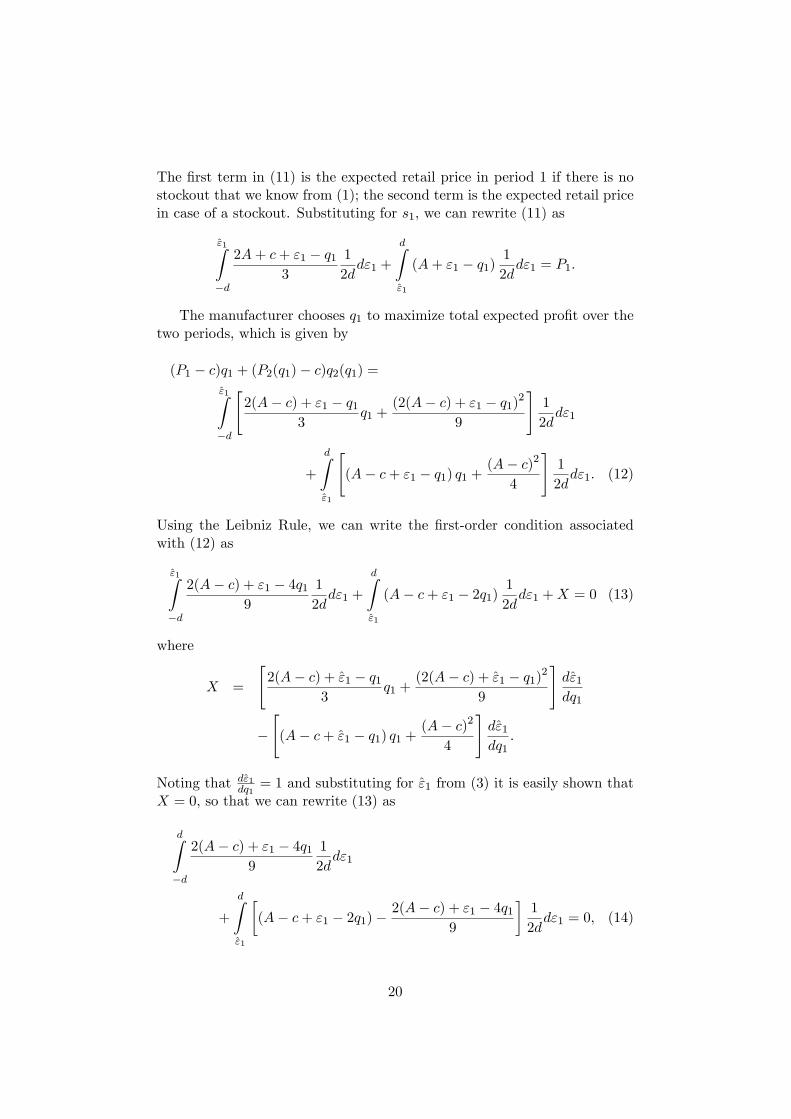
The �rst term in (11) is the expected retail price in period 1 if there is nostockout that we know from (1); the second term is the expected retail pricein case of a stockout. Substituting for s1, we can rewrite (11) as

"̂1Z�d

2A+ c+ "1 � q13

1

2dd"1 +

dZ"̂1

(A+ "1 � q1)1

2dd"1 = P1:

The manufacturer chooses q1 to maximize total expected pro�t over thetwo periods, which is given by

(P1 � c)q1 + (P2(q1)� c)q2(q1) ="̂1Z�d

"2(A� c) + "1 � q1

3q1 +

(2(A� c) + "1 � q1)2

9

#1

2dd"1

+

dZ"̂1

"(A� c+ "1 � q1) q1 +

(A� c)2

4

#1

2dd"1: (12)

Using the Leibniz Rule, we can write the �rst-order condition associatedwith (12) as

"̂1Z�d

2(A� c) + "1 � 4q19

1

2dd"1 +

dZ"̂1

(A� c+ "1 � 2q1)1

2dd"1 +X = 0 (13)

where

X =

"2(A� c) + "̂1 � q1

3q1 +

(2(A� c) + "̂1 � q1)2

9

#d"̂1dq1

�"(A� c+ "̂1 � q1) q1 +

(A� c)2

4

#d"̂1dq1

:

Noting that d"̂1dq1 = 1 and substituting for "̂1 from (3) it is easily shown thatX = 0, so that we can rewrite (13) as

dZ�d

2(A� c) + "1 � 4q19

1

2dd"1

+

dZ"̂1

�(A� c+ "1 � 2q1)�

2(A� c) + "1 � 4q19

�1

2dd"1 = 0; (14)

20

which, after simpli�cation, becomes the �rst-order condition (4) in the mainbody of the paper.

After substitution for "̂1 and integration we can rewrite (14) to obtain

(A� c+ 4d� 2q1) (5 (A� c) + 2d� 10q1) = 0:

There are two solutions: q1 = 12 (A� c)+

15d and q1 =

12 (A� c)+ 2d. Since

we require d > "̂1 = q1 � 12 (A� c), only the �rst solution is valid. Hence

�qr1 =1

2(A� c) + 1

5d:

Using this level of output we obtain "̂1 = 15d. The probability of a stockout

can then be computed asd� 1

5d

2d = 0:4.

7.4 Proof of Proposition 4

The expected second-period output can be computed using q2 =A�c�(q1�s1)

2if q1 > s1, and q2 = A�c

2 if there is a stockout. This implies:

E (�qr2) =

"̂1Z�d

�2(A� c)� q1 + "1

3

�1

2dd"1 +

dZ"̂1

�A� c2

�1

2dd"1 (15)

=1

2(A� c)� 3

25d: (16)

Total expected output is thus given by �qr1 + E (�qr2) =

12 (A� c) +

225d.

The manufacturer�s total expected pro�t can be computed as

"̂1Z�d

"2(A� c) + "1 �

�12 (A� c) +

15d�

3

�1

2(A� c) + 1

5d

�#1

2dd"1

+

"̂1Z�d

"�2(A� c) + "1 �

�12 (A� c) +

15d��2

9

#1

2dd"1

+

dZ"̂1

"�A� c+ "1 �

�1

2(A� c) + 1

5d

���1

2(A� c) + 1

5d

�+(A� c)2

4

#1

2dd"1;

which simpli�es to

E (�r) = E (~�r) +d2

25: (17)

21

7.5 Proof of Proposition 5

Using s1 + s2 = q in (5), we obtain s1 = (2q + "1) =4 and s2 = (2q � "1) =4.After observing "1, the total expected revenue of the intermediary, E(R) =w1s1 + w2s2, is given by

E(R) = (A� s1 + "1) s1 + (A� s2) s2;

= (A� q)q + 18(2q + "1)

2 :

Prior to observing "1, the intermediary chooses q to maximizeZ d

�d

�(A� q)q + 1

8(2q + "1)

2

�1

2dd"1 � (P + cw) q � T:

From the �rst-order condition,Z d

�d

�A� q + "1

2

� 12dd"1 � (P + cw) = 0;

we obtain the optimal order quantity q = A�(P + cw) and the total expectedpro�t of the intermediary of

[A� (P + cw)]2

2+d2

24� T:

The manufacturer optimally sets P = c, and extracts the intermedi-ary�s pro�t through the transfer T . This yields the manufacturer�s expectedoutput ~qi and the expected pro�t E

�~�i�.

7.6 Proof of Proposition 6

We have to distinguish between two cases: one where q2 > 0 and one whereq2 = 0. Suppose �rst that q2 > 0. In period 2 after "2 has been revealed andgiven a wholesale price w2, retailers sell an amount s2 such that the retailprice in period 2 equals their marginal cost, that is (A� s2 + "2) = w2.The intermediary has to order goods in period 2 before observing "2. Usings2 = q2+(q1�s1), the intermediary�s expected pro�t maximization problemin period 2 can be written as

maxq2(A� q2 � q1 + s1 � cw)(q2 + q1 � s1)� P2q2 � T2;

Solving the respective �rst-order condition, A� 2q2 � 2q1 + 2s1 = P2 + cw,yields as solution a quantity

q2 =A� P2 � cw

2� (q1 � s1);

22

and an expected retail price equal to

E(p2) =A+ P2 + cw

2:

The intermediary�s expected pro�t in period 2 can then be calculated as

�int2 =

�A+ P2 + cw

2� cw

�A� P2 � cw

2

�P2�A� P2 � cw

2� (q1 � s1)

�� T2

=(A� P2 � cw)2

4+ P2(q1 � s1)� T2:

The manufacturer chooses (P2; T2) such that T2 extracts the intermedi-ary�s expected period-2 pro�t net of the intermediary�s outside option, �out,and P2 maximizes

maxP2

�(P2 � c)

�A� P2 � cw

2� (q1 � s1)

�+(A� P2 � cw)2

4+ P2(q1 � s1)� �out

):

From the corresponding �rst-order condition we obtain the manufacturer�soptimal choice P2 = c.

In period 1, after "1 has been revealed, the intermediary sets a wholesaleprice w1 and retailers purchase and sell quantity s1, such that (A� s1 + "1) =w1. The intermediary�s revenue hence is equal to (A� s1 + "1) s1 and thecorresponding marginal pro�t in period one isMR1�cw = A�2s1+"1�cw.

The intermediary�s inter-temporal arbitrage condition is that MR1 �cw =

dOutd(q1�s1) , that is, a unit sold in period 2 instead of period 1 has to yield

the same marginal pro�t as one sold in period 1, where the intermediary�spro�t in period 2 is determined by its outside option, as the rest is extractedby the manufacturer through T2. We hence have

A� 2s1 + "1 = A� 2(q1 � s1); (18)

which is identical to (5) if q1 = ~qi.The intermediary�s total expected pro�t is given by

E�(A� s1 + "1 � cw) s1 � P1q1 � (T1 � �out)

;

where we note that the manufacturer can extract �out in period 1. Using(18) to obtain s1 and substituting for �out from (6), we can rewrite theintermediary�s expected pro�t as

E

��A+

"12� q12� cw

�q1 +

"218� P1q1 � T1

�:

23

The intermediary maximizes this pro�t by ordering a quantity equal to q1 =A� P1 � cw and earns an expected pro�t of

E

((A� P1 � cw)2

2+"12(A� P1 � cw) +

"218� T1

):

It is now straightforward to show that the manufacturer chooses a two-parttari¤ such that P1 = c and T1 extracts the intermediary�s pro�t. Thus thequantity shipped to the intermediary by the manufacturer in period 1 is thesame as without re-ordering, namely �qi1 = A� c� cw.

Next suppose that q2 = 0. In this case we know from the proof of theprevious proposition that �qi1 = ~qi = A� c� cw.

7.7 Proof of Proposition 7

The manufacturer�s expected pro�t with intermediation and re-ordering canbe written as the sum of the expected pro�t in period 1 and in period 2 andthus asZ d

�df(A� c� cw)

2

2+ (A� c� cw)

"12+"218g 12dd�1

+

Z d

0f((A� c� cw)

2

4+ c(q1 � s1)� �outg

1

2dd�1;

where the �rst line corresponds to the expected total revenue of the inter-mediary in period 1 and the second line corresponds to the total expectednet revenue of the intermediary given that an order is placed only if the

realization of demand in period 1 is above average. Using s1 =�qi12 +

"14 ,

�qi1 = A� c� cw, (6) yields the desired result.

7.8 Proof of Proposition 11

With retailer-controlled inventory consumer surplus is given by:

CSr =1

2E [(A� p1) s1] +

1

2E [(A� p2) s2]

=1

2E [(s1 � "1) s1] +

1

2Eh(s2)

2i

24

where1

2E [(s1 � "1) s1]

=1

2

15dZ

�d

A� c� "1

3+

�12 (A� c) +

15d�

3

!

� A� c+ 2"1

3+

�12 (A� c) +

15d�

3

!1

2dd"1

+1

2

dZ15d

��1

2(A� c) + 1

5d� "1

��1

2(A� c) + 1

5d

��1

2dd"1

=1

2

15dZ

�d

��15(A� c) + 2d� 10"1

30

��15(A� c) + 2d+ 20"1

30

��1

2dd"1

+1

2

dZ15d

��5(A� c) + 2d� 10"1

10

��1

2(A� c) + 1

5d

��1

2dd"1

=1

8(A� c)2 � 1

50d (A� c)� 9

250d2;

and1

2Eh(s2)

2i

=1

2

15dZ

�d

A� c+ 2

3

�12 (A� c) +

15d�� A�c+2"1

3

2

!21

2dd"1

+1

2

dZ15d

�A� c2

�2 12dd"1

=1

2

15dZ

�d

�15(A� c) + 2d� 10"1

30

�2 12dd"1 +

1

2

dZ15d

�A� c2

�2 12dd"1

=1

8(A� c)2 + 3

50d(A� c) + 2

125d2

Hence we can rewrite consumer surplus as

CSr =1

8(A� c)2 + 1

8(A� c)2 � 1

50d (A� c) + 3

50d(A� c)� 9

250d2 +

2

125d2

=1

4(A� c)2 + 1

25(A� c) d� 1

50d2

25

Now consider inventory control by an intermediary and assume thatcw = 0. Consumer surplus is then given by

CSi =1

2E [(s1 � "1) s1] +

1

2Eh(s2)

2i

where

1

2E [(s1 � "1) s1] =

1

2

dZ�d

�A� c2

� 3"14

��A� c2

+"14

�1

2dd"1

=1

8(A� c)2 � 1

32d2

1

2Eh(s2)

2i=

1

2

0Z�d

�A� c2

� "14

�2 12dd"1 +

1

2

dZ0

�A� c2

�2 12dd"1

=1

8(A� c)2 + 1

32d(A� c) + 1

192d2

HenceCSi =

1

4(A� c)2 + 1

32d(A� c)� 5

192d2:

We �rst can show that for cw = 0 consumer surplus when retailers con-trol inventory exceeds consumer surplus when inventory is controlled by anintermediary

CSr � CSi = 1

25(A� c) d� 1

50d2 �

�1

32d(A� c)� 5

192d2�> 0:

Now we compute social welfare.

SW r = CSr + E (��r) =1

4(A� c)2 + 1

25(A� c) d� 1

50d2 +

(A� c)2

2+d2

25

=3

4(A� c)2 + 1

25d(A� c) + 1

50d2

SW i = CSi + E (��i) =1

4(A� c)2 + 1

32d(A� c)� 5

192d2 +

(A� c)2

2+5d2

96

=3

4(A� c)2 + 1

32d(A� c) + 5

192d2

SW r � SW i =3

4(A� c)2 + 1

25d(A� c) + 1

50d2

��3

4(A� c)2 + 1

32d(A� c) + 5

192d2�

=7

800d(A� c)� 29

4800d2 =

d [42(A� c)� 29d]4800

> 0

We thus obtain SW r > SW i for all admissible d even if cw = 0.

26

References

[1] Arrow, Kenneth, Theodore Harris and Jacob Marschak, 1951. OptimalInventory Policy, Econometrica 25, 522-52.

[2] Belavina, Elena and Karam Girotra, 2012. The Bene�ts of Decentral-ized Decision-making in Supply Chains, INSEAD WP 79.

[3] Bulow, Jeremy, 1982. Durable Goods Monopolist, Journal of PoliticalEconomy 90, 314-332.

[4] Clark, Andrew and Herbert Scarf, 1960. Optimal Policies for a Multi-Echelon Inventory Problem, Management Science 6, 475-90.

[5] Deneckere, Raymond, Howard P. Marvel, and James Peck, 1996. De-mand Uncertainty, Inventories, and Resale Price Maintenance. Quar-terly Journal of Economics 111(3), 885-913.

[6] Deneckere, Raymond, Howard P. Marvel, and James Peck, 1997. De-mand Uncertainly and Price Maintenance: Markdowns as DestructiveCompetition, American Economic Review 87(4), 619-41.

[7] Dudine, Paolo, Igal Hendel and Alessandro Lizzeri, 2006. Storable GoodMonopoly: The Role of Commitment. American Economic Review96(5), 1706-1719.

[8] Economist, 2015. Dry Run: Making Towels in India, July 11.

[9] Foster, Thomas and Richard Armstrong, 2004. Top 25 ThirdParty Logistics Providers Extend Their Global Reach, SupplyChain Brain, http://www.supplychainbrain.com/content/sponsored-channels/kenco-logistic-services-third-party-logistics/single-article-page/article/top-25-third-party-logistics-providers-extend-their-global-reach/

[10] Govindam, Kannan, 2013, Vendor-Managed Inventory: A Review basedon Dimensions, International Journal of Production Research 51(13),3808-35.

[11] Hornok, Cecilia and Miklos Koren, 2015. Per Shipment Costs and theLumpiness of International Trade, Review of Economics and Statistics97(2), 525�530.

[12] Krishnan, Harish and Ralph Winter, 2011. The Economic Founda-tions of Supply Chain Contracting, Foundations and Trends in Tech-nology, Information and Operations Management 5, 3-4, 147-309,http://dx.doi.org.proxy.lib.sfu.ca/10.1561/0200000029

27

[13] Krishnan, Harish and Ralph Winter, 2010. Inventory Dynamics andSupply Chain Coordination, Management Science 56(1), 141-147.

[14] Krishnan, Harish and Ralph Winter, 2007. Vertical Control of Priceand Inventory, American Economic Review 97(5), 1840-57.

[15] Kropf, Andreas and Philip Sauré, 2014. Fixed Costs per Shipment,Journal of International Economics 92(1), 166-184.

[16] Mateen, Arqum and Ashis K. Chatterjee, 2015. Vendor-Managed Inven-tory for Single-Vendor Multi-Retailers Supply Chains, Decisions Sup-port Systems 70, 31-41.

[17] Netessine, Sergei and Nils Rudi, 2004. Supply Chain Structures on theInternet and the Role of Marketing-Operations Interaction. In DavidSimchi-Levi; David Wu and Zuo-Jun Maz Shen (eds.), Handbook ofQuantitative Supply Chain Analysis: Modeling in the E-business Era,Kluwer Academic Publishers.

[18] PRWeb, 2012. �Ankaka Wholesale Announces New Plans forEasy Wholesale Dropshipping Anywhere�, Press release, Nov 26,http://www.prweb.com/releases/2012/11/prweb10167398.htm

[19] PRWeb, 2006. �Consumer Electronics Importers Going StraightTo The Source In China at Chinavasion.com�, August 23,http://www.prweb.com/releases/china/wholesale/prweb427625.htm

[20] Randall, Taylor, Netessine, Sergei and Nils Rudi, 2006, An EmpiricalExamination of the Decision to Invest in Ful�llment Capabilities: AStudy of Internet Retailers, Management Science 52(4), 567-80.

[21] Randall, Taylor, Netessine, Sergei and Nils Rudi, 2002. Should youtake the virtual ful�llment path? Supply Chain Management Review,November/December, 54-58.

[22] Spulber, Daniel, 1999, Market Microstructure: Intermediaries and theTheory of the Firm, Cambridge University Press.

[23] Tirole, Jean, 1988. The Theory of Industrial Organization, MIT Press,Cambridge (Mass.).

[24] World Bank, 2014. Logistics Performance Index, Report, WashingtonD.C.

28