Retrospective Theses and Dissertations Iowa State University Capstones, Theses andDissertations

1964

A theoretical investigation of heat transfer to fluidsin laminar flow in tubesKermit Layton HolmanIowa State University

Follow this and additional works at: https://lib.dr.iastate.edu/rtd

Part of the Chemical Engineering Commons, and the Oil, Gas, and Energy Commons

This Dissertation is brought to you for free and open access by the Iowa State University Capstones, Theses and Dissertations at Iowa State UniversityDigital Repository. It has been accepted for inclusion in Retrospective Theses and Dissertations by an authorized administrator of Iowa State UniversityDigital Repository. For more information, please contact digirep@iastate.edu.

Recommended CitationHolman, Kermit Layton, "A theoretical investigation of heat transfer to fluids in laminar flow in tubes " (1964). Retrospective Theses andDissertations. 2991.https://lib.dr.iastate.edu/rtd/2991

This dissertation has been 64—9268 microfilmed exactly as received

HOLMAN, Kermit Layton, 1935-A THEORETICAL INVESTIGATION OF HEAT TRANSFER TO FLUIDS IN LAMINAR FLOW IN TUBES.

Iowa State University of Science and Technology Ph.D., 1964 Engineering, chemical

University Microfilms, Inc., Ann Arbor, Michigan

A THEORETICAL INVESTIGATION OF HEAT TRANSFER TO

FLUIDS IN LAMINAR FLOW IN TUBES

by

Kermit Layton Holman

A Dissertation Submitted to the

Graduate Faculty in Partial Fulfillment of

The Requirements for the Degree of

DOCTOR OF PHILOSOPHY

Major Subject : Chemical Engineering

Approved:

lâjorWôrk

Head of Major Department

Dean /c f ' Graduate College

Iowa State University Of Science and Technology

Ames, Iowa

1964

Signature was redacted for privacy.

Signature was redacted for privacy.

Signature was redacted for privacy.

il

TABLE OF CONTENTS

Page

INTRODUCTION 1

LITERATURE SURVEY 6

Introduction 6

Heat Transfer to Liquid Metals 7

Theoretical Studies of Laminar-Flow Heat Transfer • 16

THEORETICAL ANALYSIS 22

Introduction 22

Mathematical Development 30

Description of Models and Mathematical Solutions 40

Model I. Constant wall heat flux -plug flow 40

Model II. Constant wall heat flux -fully-developed laminar flow 49

Model III. Constant wall temperature -plug flow 64

Model IV, Constant wall temperature -fully-developed laminar flow 69

Associated Heat or Mass Transfer Problems 74

RESULTS 79

. Calculations 79

Constant Wall Heat Flux Models 84

Model I. Plug flow 85 Model II. Fully-developed laminar flow 92 Thermal entrance region - Model I and Model II 100

ill

Page

Constant Wall Temperature Models .103

Model III. Plug flow 103 Model IV. Constant wall temperature -fully-developed laminar flow 113

Thermal entrance region - Model III and Model IV 122

DISCUSSION 126

CONCLUSIONS ' 128

RECOMMENDATIONS 130

NOMENCLATURE 132

LITERATURE CITED 137

ACKNOWLEDGMENTS 144

APPENDIX 145

Model I. Constant Wall Heat Flux - Plug Flow: Fully-developed Heat Transfer Solution 145

Computer Program Listings 149

Eigenvalues and Coefficients 174

1

INTRODUCTION

The study of transport phenomena has evolved in recent

years from a loose collection of theories and empirical

information in diverse branches of engineering and science

into a distinct subject of engineering. The transport of

heat, mass or momentum may be treated as one discipline;

however, the similarity is limited, and analysis based on

the theory of similarity applies only to the special cases

where mathematical formulation is identical. For example,

when fractional dissipation in the energy equation is not

negligible, the similarity disappears because there is no

analogous term in the momentum or mass transport equation.

A significant contribution of the transport phenomena

approach to solving engineering problems is the recognition

and accounting of the assumptions made in deriving a final

solution. Because the method of solution places emphasis

on physical principles, important factors, which were

previously neglected, are considered in the analysis. Thus,

proper application of the final results is facilitated by

emphasizing the limitations of the analysis.

In the relatively new areas of nuclear power and space

exploration, previous engineering correlations may not be

directly applicable. An example of such a situation is

that the correlations for turbulent forced convection heat

2

transfer for conventional fluids are not valid for liquid

metals. As a result, there have been numerous theoretical

and experimental investigations of turbulent-flow heat

transfer to molten metals.-

An examination of the literature on liquid metal heat

transfer applications in nuclear reactors would establish

the flows in the turbulent regime (l8). With a Reynolds

number of 2100, mercury at 200°F in a 0.50-inch I. D. tube

would have an average velocity of 320 feet/hour or approxi­

mately 0.088 feet/second. This represents an extremely low

velocity and mass flow rate and it is doubtful that heat

transfer to liquid metals in laminar flow would occur in

present reactors. However, in the future, efficient, com­

pact heat exchangers may find use in the space program. In

comparison to conventional heat transfer media, less benefit

is gained with liquid metals through use of fins or surface

roughening.1 For small tubes, the heat transfer coefficient

is less affected by velocity and tubes in the range of 0.10

inch I. D. and less are practical for liquid metals if the

fabrication cost can be offset by use of newer alloys.

Furthermore, as power requirements increase, and particu­

larly as a need for compact nuclear reactors develops,

^Lyon, R. N., Oak Ridge National Laboratory, Oak Ridge, Tennessee. Heat transfer to liquid metals in laminar flow. Private communication. February 26, 1962.

3

there probably'will be a trend toward use of smaller

channels in heat exchangers. As a contrast to the example

of laminar flow of mercury, molten lithium at 1200°F in

1/16-inch I. D. tubes would have an average velocity of

approximately 5 feet/second for laminar flow at a Reynolds

number of 2100.

In anticipation of the need for compact nuclear re­

actors, the Martin Company is designing 60 kw, 200 kw, and

2000 kw reactor systems (2-4, 44). These reactors, which

will use molten lithium as the coolant, are expected to be

very useful in the space program during 1970 to 1975.

Allison Division of General Motors Corporation is

working on the design, construction and operation of a

mobile military compact reactor (MCR) under a high priority

long-range nuclear program (51). The extremely mobile,

compact nuclear power plant will be capable of generating

3000 kw of electricity. The unit will have a high tempera­

ture, liquid metal-cooled reactor coupled to a power con­

version system. In addition to its military use, the MCR

could serve as a power source in civilian defense and power

failure emergencies.

Although turbulent-flow heat transfer to liquid metals

has received considerable attention, such is not the case

for the laminar flow region. The Nusselt values obtained

from experimental studies of laminar-flow heat transfer to

4

liquid metals do not agree well with the expected Nusselt

values based on theoretical calculations. Recent work in

Russia (57) has helped to clarify the anomaly from the

experimental viewpoint; however, the validity of the so-

called theoretical analyses may be questioned.

The main purpose of this investigation was to examine

theoretically the heat transport process to a fluid in plug

flow or fully-developed laminar flow in a tube with a pre­

scribed wall boundary condition. In the analysis, the

axial heat conduction term, which has been neglected in

most previous studies, was included. Although the results

are general and apply to most fluids, emphasis was placed

on application to liquid metals as heat transfer media. A

second purpose of this study was to provide theoretical and

computational information on a method of solution of a

generalized Sturm-Liouville differential equation system.

Extensions of the method of solution are discussed for

similar heat transport problems which contain uniform heat

generation, viscous dissipation, and other forms of the

velocity profile. The analogy between heat and mass trans­

port is presented and possible treatments of chemical engi­

neering kinetics problems are discussed.

This work may be divided into two parts, depending on

the form of the wall boundary condition employed. In the

first part, the heat transport problem was considered for

5

a wall boundary condition of constant wall heat flux and

either plug flow or fully-developed laminar flow velocity

profile. The second part was a treatment of the heat

transport problem with a wall boundary condition of con­

stant wall temperature and either plug flow or fully-

developed laminar flow velocity profile. The important

heat transfer parameters for these ideal models should

provide preliminary information for estimating the heat

transfer associated with more physically realizable wall

boundary conditions and velocity profiles in both laminar

and turbulent flow at low Peclet numbers.

6

LITERATURE SURVEY

< Introduction

In the past decade the amount of heat transfer re­

search has increased considerably because of the demands

presented by new technologies associated with nuclear

power and space exploration. Much of the literature on

heat transport is discussed in books by Bird _et al. (5),

Grôber _et al. (25), Jakob (32, 33), and others (20, 37, 38,

49, 59). The book by Bird _et _al. (5) presents the most .

complete and rigorous analysis of the transport processes,

whereas the other books provide more detailed reviews of

the important heat transfer work. The text by Grôber

et al. (25) gives an excellent summary of the heat transfer

research conducted in Europe.

A detailed review of the status of heat transfer re­

search will not be presented here. Rather, the discussion

will be limited to the pertinent experimental and theoreti­

cal heat transfer studies which contribute to the theory

of heat transport to liquid metals in laminar and transition

flow. For more information on the experimental studies of

liquid metal heat transfer, the liquid-metals handbooks

(31, 39, 46) and review articles (10, 45) may be consulted.

7

Heat Transfer to Liquid Metals

In the early investigations of heat transfer to liquid

metals, a discrepancy was observed between the experimental

measurements of heat transfer coefficients and those pre­

dicted from theory. It was postulated that the anomaly

was due to poor wetting of the heat transfer surface by

the liquid metal because a meter reading was not obtained

with the electromagnetic flowmeter unless the liquid metal

wetted the conduit wall. Hence, a similar phenomenon was

presumed to be affecting the heat transport. In a discus­

sion of the wetting effect, Quittenton and MacDonald (58)

showed that a small amount of adsorbed gas on the surface

of the conduit would provide a large electrical resistance.

This explained why the flowmeter readings were not detected

when wetting was not present. However, for a typical liquid

metal heat transfer experiment, the calculated temperature

drop across the adsorbed gas layer was small, and therefore,

the gas layer provided a low resistance to heat transfer.

Therefore, wetting of the conduit wall by the liquid metal

has little effect on forced convection heat transfer. This

observation should not be construed to apply directly to

other operations such as the condensation of metal vapor.

Stromquist (69) and Chelemer (12) investigated the

effects of wetting and gas entrainment on the heat transfer

8

to mercury in turbulent flow. It was found that entrained

gas in the liquid metal has a deleterious effect on the

heat transfer performance. This phenomenon is analogous

to the effect produced by the presence of air in many com­

mon insulation materials.

Johnson _et al. (34) observed a discrepancy between the

experimental and theoretical Nusselt values for forced con­

vection heat transfer to liquid metals in laminar flow.

The experimental Nusselt numbers were considerably lower

than the theoretical Nusselt number of 4.364 for constant

wall heat flux with fully-developed laminar flow. Using

lead-bismuth and mercury as heat transfer media, the ex­

perimental Nusselt numbers decreased from approximately 6

at a Reynolds number of 10,000 down to approximately 1 at

a Reynolds number of 1200. Gas entrainment, distortion of

the velocity profile, and variation of the physical proper­

ties were considered too small to account for the error

between the experimental and theoretical Nusselt numbers.

A recent heat transfer study in Russia by Petukhov and

Yushin (57) concluded that the anomaly reported by Johnson

et al. (34) was due to not accounting for axial heat con­

duction in the fluid and the tube wall. In an investiga­

tion of heat transfer to mercury in the laminar and transi­

tion flow regions, the experimental heat transfer results,

which were calculated from measured values of temperature,

9

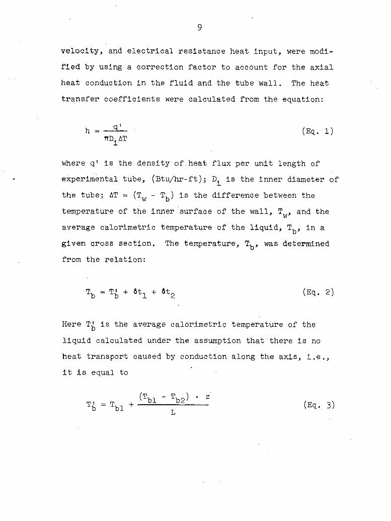
velocity, and electrical resistance heat input, were modi­

fied by using a correction factor to account for the axial

heat conduction in the fluid and the tube wall. The heat

transfer coefficients were calculated from the equation:

where q1 is the density of.heat flux per unit length of

experimental tube, (Btu/hr-ft); is the inner diameter of

the tube; AT = (T - T, ) is the difference between the x w D

temperature of the inner surface of the wall, T^, and the

average calorimetric temperature of the liquid, T^, in a

given cross section. The temperature, T^, was determined

from the relation:

Here T^ is the average calorimetric temperature of the

liquid calculated under the assumption that there is no

heat transport caused by conduction along the axis, i.e.,

it is equal to

(Eq. 1) TTD, AT 1

(Eq. 2)

, (?bl ' ?b2) ' = (Eq. 3)

L

10

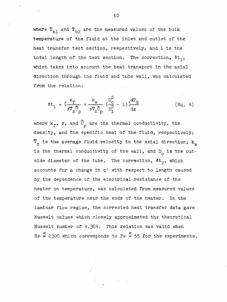
where T^-and are the measured values of the bulk

temperature of the fluid at the inlet and outlet of the

heat transfer test section, respectively, and L is the

total length of the test section. The correction, 6t^,

which takes into account the heat transport in the axial

direction through the fluid and tube wall, was calculated

from the relation:

k„ k , dT^ 6tl = t _ a + _ /s 5 " i) — (Eq. 4)

pV,Cp dz

A where k^, p, and C are the thermal conductivity, the

density, and the specific heat of the fluid, respectively;

Vz is the average fluid velocity in the axial direction; k^

is the thermal conductivity of the wall, and Dq is the out­

side diameter of the tube. The correction, &tg, which

accounts for a change in q1 with respect to length caused

by the dependence of the electrical resistance of the

heater on temperature, was calculated from measured values

of the temperature near the ends of the heater. In the

laminar flow region, the corrected heat transfer data gave

Nusselt values which closely approximated the theoretical

Nusselt number of 4.364. This relation was valid when

Re = 2300 which corresponds to Pe = 55 for the experiments.

11

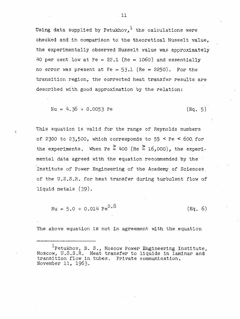
Using data supplied by Petukhov,1 the calculations were

checked and in comparison to the theoretical Nusselt value,

the experimentally observed Nusselt value was approximately

40 per cent low at Pe = 22.1 (Re = 1060) and essentially

no error was present at Pe .= 53.1 (Re = 2250). For the

transition region, the corrected heat transfer results are

described with good approximation by the relation:

Nu =4.36 + 0.0053 Pe (Eq. 5)

This equation is valid for the range of Reynolds numbers

of 2300 to 23,500, which corresponds to 55 < Pe < 600, for

the experiments. When Pe = 400 (Re = 16,000), the experi­

mental data agreed with the equation recommended by the

Institute of Power Engineering of the Academy of Sciences

of the U.S.S.R. for heat transfer during turbulent flow of

liquid metals (39).

Nu = 5.0 + 0.014 Pe0,8 (Eq. 6)

The above equation is not in agreement with the equation

^Petukhov, B. S., Moscow Power Engineering Institute, Moscow, U.S.S.R. Heat transfer to liquids in laminar and transition flow in tubes. Private communication. November 11, 1963.

12

Nu = 7.0 + 0.025 Pe 0 .8 (Eq. 7)

which is recommended by the Liquid-Metals Handbook (46),

nor is it in agreement with the equation

which, according to Lubarsky and Kaufman (45), describes

the previous experimentally observed Nusselt values for

turbulent-flow heat transfer to liquid metals with a wall

boundary condition of constant heat flux.

The analysis given by Petukhov and Yushin is in theo­

retical agreement with the development given by Trefethen

(71). The latter work was concerned with the meaning of

the concept of "mean temperature" for a fluid passing a

given section of a tube being heated. Defining the "energy

mean temperature" to be that temperature representing an

average energy per unit volume which, when multiplied by

the total volume of fluid passing a section in a period of

time, equals the energy of the fluid as it passed the

section. This definition leads to the relation

Nu = 0.625 Pe0,8 (Eq. 8)

T energy (Eq. 9)

13

Assuming steady state and no entry effects at the section,

an energy balance gives

_TTD? A

OVinletV-^ AT " "CvJ,ATJVT-V-i1A>'1t + WT.

+ k jI^aT+kwjT"(Do-Dl) ,T.0

dz 4 dz 4

(Eq. 10)

Combining the above two equations gives an equation for the

energy mean temperature in terms of commonly measured

values.

n2 _ 2

t = T _j H + i _|_ k ( 2 i ) ] energy inlet pç vrrD2/4 p C V f w D? dz

v v i

(Eq. 11)

Probes for measuring velocity and temperature provide

another method to measure mean temperature. Assuming that

a probe can measure exactly the values T and V, the "probe

mean temperature" at a section is

f . T V d A (Eq. 12)

probe j . aA A

This definition of mean temperature is usually employed in

analyses predicting heat transfer coefficients. If

V . dA = (V + v)dA and T = T + t, a relationship between

probe and energy mean temperature is obtained

14

J\ - t•v dA Tprobe ~ Tenergy + "J^dA Eq'

The average over a period of time of the product, t*v, does

not vanish; it represents the turbulent or eddy diffusion

of heat in the axial direction. The "mixing-box mean

temperature" at a section is the temperature which would

be measured in a mixing box inserted at that section. An

energy balance gives

Tm.b. ' Tlnlet + pg *d£/4 (Eq' 141

Combining Equations 11 and 14,

D2 - D2

Tenergy = Tm.b. + pg kf + kw ^ ^2 ^ ~ (Eq* 15'

The last term in the above equation is the correction

factor, 6t^, which was added to the measured fluid tempera­

ture by Petukhov and Yushin. A Nusselt number based on

mixing-box mean temperature is usually used for reporting

experimental data. Because of the various definitions of

mean temperature, the Nusselt values based on mixing-box

and probe mean temperatures will not be the same. Trefethen

defined a ratio, K, to be

15

K • — + — (°^A) + P6V - (tfA (Eq. 16) k~ k_ 3T TTDf 1 1 1 k _ ± -

f dz 4

and then using the definitions of mean temperature, Num ^ ,

NuprobeJ and Pe, the following relationship was derived.

Nu„ v = ""probe (Eq. 17)

" 1 ^ "Vobe Pe2

For laminar flow, Tprote - Tenergy, and Nuprote - 48/11,

therefore, Equation 18 reduces to

Nu. m.b. (48/11) (Eq. 18)

1 + 4K(48/11 )

Pe%

At a low value of the Peclet number and a relatively

high value of K, i.e., K = 50 to 100, the experimentally

measured fully-developed Nusselt number, Num ^ , would be

significantly less than the so-called theoretical value of

48/11 = 4.364. Hence, by not accounting for axial conduc­

tion in the fluid and the tube wall at low Peclet values,

the experimental Nusselt values may be considerably less

than the theoretical Nusselt value of 4.364. This conclu­

sion is in agreement with the work of Petukhov and Yushin.

16

It should be noted that the analysis given by Trefethen

and the analysis given by Petukhov and Yushin are limited

ST to fully-developed heat transport where is a constant

and do not apply to the thermal entry region.

It can be concluded that for turbulent and laminar

flow heat transport to liquid metals at low Peclet numbers,

precautions must be taken in the design and operation of

experimental apparatus, and in the interpretation of the

results obtained. Also, the use of theoretical forced con­

vection heat transfer analyses should be checked by the

above method to obtain valid data for design calculations.

Theoretical Studies of Laminar-Plow Heat Transfer

Heat transport to a fluid in fully-developed laminar

flow in a tube with uniform wall temperature has been

treated analytically, first by Graetz (22) and later by

Nusselt (53). The results of Nusselt have been recalcu­

lated and to somewhat some extent improved by Jakob (32).

Abramowitz (l) and Brown (ll) have determined with high

accuracy the eigenvalues for the limiting case of large

Peclet number. Mercer (48) calculated thermal profiles

near the inlet of the tube. Kays (36) treated the heat

transport problem numerically and obtained results in

agreement with the analytical solutions. The analysis was

17

made for Pr = 0.7 and it is strictly applicable only to

air or common gases. Pahor and Strnad (54, 55) and

Labuntsov (40) presented analyses which indicate that the

asymptotic Nusselt number is a function of the Peclet num­

ber for a tube with constant wall temperature. As the

Peclet number approaches zero, the asymptotic Nusselt num­

ber approaches 4.18, but as the Peclet number becomes

large, the asymptotic Nusselt number approaches 3.656.

Sellars et al. (64) developed a solution for arbitrary

wall temperature with fully-developed laminar flow and

Whiteman and Drake (73) extended the work to arbitrary

forms of the velocity profile. Yih and Cermak (75), Schenk

and Dumore (6l), and Rosen and Scott (60) treated the

problem for which the tube wall has a finite wall trans-

missivity. Brinkman (9) and Schenk and Van Laar (62)

accounted for viscous dissipation in non-Newtonian fluids.

Topper (70) extended the Graetz-Nusselt. problem to account

for uniform heat generation.

Goldstein (21) derived the asymptotic solution for

heat transfer to a fluid in fully-developed laminar flow

in a tube with constant wall heat flux. Eagle and

Ferguson (19) obtained an equivalent result for the case

where the wall temperature varies linearly For either of

these models, an asymptotic Nusselt number of 48/11 or

4.364 is obtained. Sellars et al. (64) extended the Graetz

18

solution to arbitrary wall heat flux and Whiteman and

Drake (73) applied the results to arbitrary forms of the

velocity profile. Siegel _et al. (65) used a method of

superposition to determine the heat transfer in the

thermal entrance region at large Peclet values for a tube

with constant wall heat flux. The definition of thermal

entrance region used was the tube length necessary for the

local Nusselt number to approach within 5 per cent of the

asymptotic Nusselt number. This definition is not accepted

universally; however, it is adequate for most engineering

calculations. Independently, Akins and Dranoff (3) derived

a similar solution and the eigenvalues and coefficients

computed by Dranoff (17) are in agreement with those pre­

sented by Siegel _et _al. Noyes (52) used the results of

Siegel et al. to derive an integrated closed form solution

for the variation of the heat transfer coefficient for an

arbitrary heat flux distribution along the length of the

tube.

In all of the heat transfer work briefly mentioned

above, the effect of axial heat conduction has been

neglected. Schneider (63) made a theoretical study of

heat transfer for plug flow in ducts and tubes with uni­

form wall temperature and included the axial conduction

term in the solution of the energy equation. It was con­

cluded that the axial conduction effect may be considered

19

negligible provided that the Peclet number is greater than

100. Furthermore, the over-all effects of axial conduction

are concentrated in the thermal entry region of the conduit,

and as such it does not influence the local heat transport

in the downstream region of thermally established flow. In

other words, the local asymptotic Nusselt numbers are the

same either in the presence or in the absence of axial heat

conduction. But since the axial conduction does affect the

local heat transport in the entrance region, the integrated

or average heat transport is distinctly different if this

effect is taken into account.

Millsaps and Pohlhausen (50) present an analysis which

includes the effects of axial heat conduction and viscous

dissipation for fully-developed laminar flow in a tube with

uniform wall temperature. The method of solution used was

an eigenfunction expansion in terms of Bessel functions fol­

lowed by a numerical approximation of the eigenvalues. Four

eigenvalues and eigenfunctions were determined for various

Peclet numbers; however, Nusselt numbers, mixed-mean tem­

peratures, and thermal entry lengths were not calculated.1

Independently, Singh (66, 67) developed an equivalent solu­

tion patterned after the theoretical analyses given by

^Mi11saps, K., University of Florida, Gainesville. Analysis of heat transfer for Poiseuille flow in a tube. Private communication. November 13, 1963.

20

Dennis (l4).and Dennis and Foots (15). The Nusselt values

and mixed-mean dimensionless temperatures in the entrance

region were calculated for the limiting case of a large

Peclet number. Also, Singh pointed out that the method of

solution can be worked out with viscous dissipation and any

prescribed heat generation included. Abramowitz _et <al. (2)

employed a Runge-Kutta technique.to numerically integrate

the differential equation obtained by separation of the

variables. The eigenvalues and expansion coefficients

were tabulated for several Peclet numbers and checked with

those given by Millsaps and Pohlhausen (50). The corre­

sponding eigenfunctions were not tabulated. The eigen­

values at a Peclet number of 1000 checked closely with

those for the limiting case of large Peclet number as 'given

by Brown (ll) and Abramowitz (l).

For the constant wall temperature problem with fully-

developed laminar flow, Labuntsov (40) briefly considered

including the axial conduction term and concluded that the

asymptotic Nusselt number is a function of the Peclet num­

ber as given by Pahor and Strnad (54, 55). However, for

the constant wall heat flux problem with axial conduction

included, Labuntsov concluded that the asymptotic Nusselt

number does not depend on the value of the Peclet number.

Petukhov and Tsvetkov (56) analyzed the constant wall

heat flux problem by dividing the fluid into three

21

concentric cylindrical shells and solved numerically the

resulting system of linear second order differential equa­

tions. The treatment parallels the simple model given by

Seban in a discussion of the paper by Trefethen (71). Al­

though the solution development is approximate, it illus­

trates the effect of axial heat conduction of heat trans­

port in the thermal entry region.

22

THEORETICAL ANALYSIS

Introduction

By applying the first law of thermodynamics to an open

system, the equation of energy may be derived. A rigorous

derivation is presented by Bird_et al. (5) and the resulting

equation in terms of the.fluid temperature is

P K T5E = ' V - T(||)v V .v - T : vv + G (Eq. 19)

Assuming the fluid to be incompressible (V-V = 0) and

flowing at steady state, Equation 20 is obtained.

PC V.VT = - v-q - t: VV + G (Eq. 20)

The first term of the equation represents the rate of gain

of internal energy per unit volume. It is regarded as the

forced convection term because of the presence of the

velocity vector. The last three terms of the equation

represent the rate of internal energy input by conduction

per unit volume, the irreversible rate of internal energy

increase per unit volume by viscous dissipation, and the

rate of increase of internal energy per unit volume by a

uniformly distributed energy source, respectively.

23

In like manner, the equation of motion may be derived

by making a momentum balance for an open system (5).

DV P — = - V P - V - T + P £ (Eq. 21) Dt ~

Assuming steady state,

pV . 7V = - VP - V % + Pg (Eq. 22)

In this form, the equation of motion states that a small

volume element moving with the fluid is accelerated because

of the forces acting upon it.

In general, the fluid properties of density and vis­

cosity exhibit some dependence on temperature, and the

energy transport depends on the fluid velocity. Hence, a

solution to a heat transport problem involving fluid motion

would entail a simultaneous solution of the equations of

motion and energy. Such a solution is usually difficult

and tedious; consequently, the velocity profile is assumed

to be of analytical form and the equation of energy is

solved independently from the equation of motion. In the

analysis two models will be used for the velocity profile,

i.e., plug flow and fully-developed laminar flow. In

reality, the velocity at any point has a radial component

for symmetric flow until fully-developed flow is reached.

24

Furthermore, it is tacitly assumed that the fluid is

Newtonian and the velocity and density are not temperature

dependent, which is not physically realizable and is

recognized as an approximation. The validity of the latter

assumptions can be tested for a specific fluid by examina­

tion of physical properties for variation with respect to

temperature.

For the plug flow model, the velocity distribution is

uniform across the radius as given by Equation 23.

= Vg (Eq. 23)

Equation 22 reduces to the Poiseuille (parabolic)

velocity distribution (5) for fully-developed laminar flow

vz = 2VzCl - (r/R)2] (Eq. 24)

where is the average fluid velocity in the axial direc­

tion.

The equation of energy for axial flow in cylindrical

coordinates (5) is

PSVz H = i h (rqr) - FW+"5/ + Trz"5FE + G (Eq- 25)

The r-momentum flux in the z direction, rz, is defined as

25

T (Eq. 26)

Similarly, the heat fluxes are defined by

a. q. lr

b. q, z

(Eq. 27)

Assuming radial symmetry, q^ = 0, and Equation 25 becomes

The last two terms in Equation 28 are designated as a heat

source from viscous dissipation and a uniform heat genera­

tion source or sink, respectively. Viscous dissipation

occurs with all fluids with finite viscosity; however, it

is usually of significance only in highly viscous fluids.

An example of a uniform heat generation source is uniformly

distributed nuclear particles giving off energy during

radioactive decay.

For. low Peclet numbers, when the axial conduction

§2|J! term, k —5, is neglected, the fluid temperature approaches

'Vz I = k[? I?

%2_ av_ ? - (a(-§~)2 + G (Eq. 28)

dz

26

the temperature of the conduit as the Peclet number

approaches zero. The order of magnitude of the Peclet

number at which the conduction effect becomes important

can be estimated from the relative magnitude of the longi­

tudinal conduction and convection terms (l6). The axial

ô^T a §m conduction is k —0 and the axial convection is pC V .

32% p z

2 The order of magnitude of these two terms are k/L and

pC V /L, where L is a characteristic order of magnitude p z

length such as tube diameter. Therefore, their ratio is

axial conduction 1 1

axial convection Pe Peclet number

This suggests that the effect of axial conduction is gener­

ally negligible for Peclet numbers exceeding 100 for which

the present theoretical analyses will be valid. The axial

conduction effect should be examined primarily in the range

0 = Pe = 100. It is interesting to note that for liquid

metals, the laminar flow region would occur generally at

Peclet numbers of 100 or less, and therefore, the axial

conduction term should be considered for such heat transfer

calculations. However, for gases, the laminar flow region

begins when the Peclet number is approximately 1500, and

previous analyses neglecting axial conduction should be

valid for heat transfer calculations even in the thermal

27

entrance region.

Before proceeding to the equation development and the

solutions for the models, a "brief discussion of the heat

transport process will provide a better understanding of

the utility and limitations of the analyses.

When a fluid enters a heated or cooled tube, the rate

at which the'hydrodynamic profile develops depends on the

viscosity. Highly viscous fluids, with large internal

friction forces, will show a rapid profile stabilization,

while low viscosity fluids support a developing or unstable

profile over many more diameters near the entrance. The

rate of temperature development, on the other hand, depends

on the thermal conductivity of the fluid, highly conducting

fluids showing rapid temperature profile stabilization.

Thus, the ratio of the rate of hydrodynamic profile develop­

ment to the rate of thermal profile development is expressed A

by the Prandtl number, Pr = |i C^/k. Therefore, for liquids

of low Prandtl number (liquid metals), the temperature pro­

file is fully established long before the velocity profile

is established. Conversely, oils having Prandtl numbers

ranging up to l600 will show a rapid stabilization of the

velocity profile and a slower temperature profile develop­

ment rate.

By neglecting axial conduction and numerically inte­

grating the equation of energy, Kays (36) obtained the

28

following equation for estimating the thermal starting

length, Lg.

L — = 0.05Pr Re = 0.05 Pe (Eq. 29) Di

Lg is the tube length necessary for the heat transfer co­

efficient to approach within 1 per cent of its fully-

developed value. Equation 29 was derived for fully-

developed laminar flow of a fluid (Pr = 0.70) in a tube

with constant wall temperature. The equation is strictly

applicable to the flow of air or common gases, but it pro­

vides a preliminary estimate of Lg for a fluid whose

Prandtl number is not 0.J0. The hydrodynamlc starting

length, L^., can be predicted from a relation given by

Langhaar ( 4l ).

Lh — = 0.05 Re (Eq. 30) Di.

is the tube length required for the center-line velocity

to reach 99 per cent of its fully-developed value. The

ratio of Equations 29 and 30 Indicates that only in a fluid

with a Prandtl number close to 0.85 will the thermal and

hydrodynamlc profiles develop at approximately the same

rate.

For fully-developed laminar flow, the velocity profile

29

(Equation 24) is parabolic. With heating, the assumption

of parabolic velocity profile would be nearly true through­

out the heat transfer region if the fluid viscosity were

not a function of temperature. Because all fluids exhibit

a temperature dependent viscosity characteristic, there

will be a viscosity gradient across the tube radius, simi­

lar to the temperature gradient. If the viscosity increases

with temperature (gases) and the wall is hotter than the

fluid, there will be a viscosity increase near the wall and

a tendency for the fluid to move radially toward the center

where the resistance to flow is less. As a result, the

original parabolic velocity distribution becomes more

pointed or elongated because the velocity increases at the

central section of the tube. For fluids which possess a

viscosity decrease (most liquids) with increased tempera­

ture, the velocity profile becomes more blunt and is inter­

mediate between the parabolic and plug flow models. The

opposite effects can be expected when cooling of the fluid

occurs. Such behavior will be present especially when high

heat fluxes are used.

When a flowing fluid is heated, density variations

occur and yield buoyancy effects which tend to distort the

velocity profile. In the analysis it is assumed that the

density is independent of temperature, a relatively good

approximation for dense fluids such as liquid metals. • If

30

the results are applied to design of heat exchangers for

use in space where there is zero gravity, buoyancy effects

would not be present.

The assumed velocity profile models, i.e., plug flow

and fully-developed laminar flow, should provide prelimi­

nary information on heat transfer characteristics for

laminar flow in tubes. Actually the plug flow model repre­

sents an upper limit for the heat transport and this may

closely approximate the velocity distribution for liquid

metals at the entrance to a tube. For liquid metals,

Pr ~ 0.01 to 0.10, and the velocity profile development is

slow in comparison to the thermal profile development.'

Mathematical Development

In most standard texts on the solution of boundary

value problems, the Sturm-Liouville equation and associated

boundary conditions are discussed in conjunction with the

solution of partial differential equations by the classical

method of separation of variables. Recently, a numerical

analysis based on a generalized Sturm-Liouville system has

been presented by Dennis and Foots (15), Dennis (l4) and

Singh (66, 67). The discussion given here will closely

parallel that of the previous presentations; however, the

solution of the heat transport models will be understood

31

more readily If the theory and numerical analysis method

are reviewed.

Consider the generalized Sturm-Liouville system:

Cp(x) X' (x) ] + Cq(x) + g(x,X)] X(x) = 0 (Eq. 31)

subject to the boundary conditions,

a^X(a)•+ a^X'(a) = 0

(Eq. 32)

bxX(b) + bgX'(b) = 0

where a^, a2, b^, and b^ are prescribed constants and X is

a characteristic parameter. The functions p(x), q(x),

g(x, X), and dg(x,X)/dX are assumed to be continuous

throughout the finite interval (a,b), and X in the last

two functions can have only the eigenvalues X^, (n = 1, 2,

3, ), to be given by Equation 32. Corresponding to

each eigenvalue, X^, there exists an eigenfunction

X(x) = Xfi(x) satisfying Equations 31 and 32, and these

eigenfunctions form a complete orthogonal set in the in­

terval (a,b ). Any piecewise continuous function defined

in this domain may be expanded as an infinite series of

these functions,

f(x) = Z a X (x) (Eq. 33) n=l n n .

32

where,

Jit-%^\=>.nf(x}xn(xïdx

(Eq. 34) a. 'n

because

/atg(x,Xn) - g(x,xm):xn(x) Xm(x) dx = 0, (m n)

(Eq. 35)

The eigenfunctions, X (x), may be normalized on the inter­

val (a,b) by dividing each X^(x) by Nn, i.e., Xn*(x) =

Xn(x)/Nfi. Without loss of generality, the normalized

eigenfunctions, Xn*(x), will be renamed in the sequel as

Xn(x) so that Equation 36 will yield N = 1. Hence, the

eigenfunctions, Xfi(x), form an orthonormal set on the

interval (a,b). Then

and

^(x)dx . n

(Eq. 36)

a n j.b[8£ixiXl^ nf(x)Xn(x)dx (Eq. 37)

The determination of eigenfunctions and eigenvalues

of Equations 31 and 32 often is difficult. Solutions are

33

obtained usually by substitution of a power series or by

techniques involving the calculus of finite differences.

Instead of using conventional methods of solution, a

numerical analysis based on Equation 33 will be employed.

. As a first step in the development of a technique to

solve Equation 31, consider the equation

where y(x) satisfies boundary conditions analogous to Equa­

tion 32 and a is a characteristic parameter. It is presumed

that the analytical solutions y = U^(x) of Equation 38

satisfying Equation 32 in the domain (a,b) can be obtained.

Um(x) is the eigenfunction corresponding to the eigenvalue,

to be determined by Equation 32 and these eigenfunc­

tions form a complete orthogonal set in the interval (a,b).

Therefore, the solution of Equation 31 satisfying the con­

dition given by Equation 32 can be expanded in terms of the

eigenfunctions, Um(x), as

•|^Cp(x)y'.] + H(x, a )y = 0 (Eq. 38)

CO

X(x) = Z C U (x) n=l

(Eq. 39)

Substitution of this series into Equation 31 produces an

infinite set of simultaneous algebraic equations from which

the coefficients, C . may be determined.

34

A special case of Equation 31, namely g(x,X) = Xg(x),

produces the original Sturm-Liouville equation, and this

combined with the boundary conditions of Equation 32 is

the conventional Sturm-Liouville system.

It arises in many physical applications where a partial

differential equation is solved by the method of separation

of variables.

can be written as Vessel's equation of order v.

CxU'(x)] + (a2x - v2/x)U(x) = 0, (a,v)real. (Eq. 4l)

This equation may be regarded as an auxiliary equation

corresponding to Equation 38 when p(x) = x. The eigenfunc­

tions satisfying Equation 4l are given by

Cp(x)X'(x)] + Cq(x) + Xg(x)]X(x) = 0 (Eq. 40)

When p(x) = x and H(x, cc ) = (a2x - v2/x), Equation 40

(Eq. 42)

where v is any integer or fraction and wn is an arbitrary

constant. The functions, Un(x), satisfy the boundary con­

ditions specified by Equation 32 if

35

alCjv(ccna) + wnYv(ana)] + a2anCjv(ana) + wnYv ana)3 = 0

(Eq. 43)

= °

where a prime denotes differentiation with respect to the

argument. For specified values of a^, ag, b^, and bg, the

positive roots of Equation 43 define the characteristic

values, a , corresponding to the eigenfunctions, Un(x).

These functions are orthogonal with respect to the weight

function, x, in the interval (a,b), hence (13, 72),

xUn(x)Um(x)dx = 0 (m n) (Eq. 44)

Ja <(x)dx = = ) = *n

nX (Eq. 45)

Now, a method of solution of Equation 31 for p(x) = x

will be developed using the auxiliary equation and ortho­

gonality relations given above. Equation 31 for p(x) = x

is

CxX(x)] + [q(x) + g(x,X)]X(x) = 0 (Eq. 46)

A solution of Equation 46 satisfying the boundary

36

conditions of Equation 32 may be expressed by an infinite

series of U (x) which are given by Equation 42.

CO

X(x) = z C u (x) (Eq. 47) n=l n n

Because Bessel's equation (Equation 4l) is satisfied by

each U (x), it is satisfied also by any linear- combination

of the Un(x). Therefore, Equation 47 also represents a

solution to Equation 4l, and substitution of Equation 47

into Equation 4l produces an identity which is valid even

for integration. Application of the orthogonality rela­

tions given by Equations 44 and 45 yields

fa xX(x)Un-(x)dx = x 2 CmU (x) -Un(x)dx = (Eq. 48) m=l

and

•Ta % [xX'(x)] - X(x)J Un(x)ax = - a^cn6n (Eq. 49)

Then, multiplying Equation 46 by U (x) and integrating from

a to b using Equations 48 and 49 gives

2 - anCnÔn + /a^*) + x~ + lX(x)Un(x)dx = 0 (Eq. 50)

n = 1, 2, 3,

37

This integral may be written as

Z Ja^(x) + 3T + g(xA) ]CmUm(x)Un(x)dx m=l rn^n (Eq. 51)

2 + J^[q(x) + + g(x,X)]CnU2(x)dx - a2ônCn = 0

or

00

% An-Cm = 0 3' ) 52) m=l nm m

where

Anm = Amn = + g(x,\) ]Um(x)Un(x)dx (Eq. 53)

and

Ann = ~ anSn + + x~ + g(xA) ]U2(x)dx (Eq. 54)

When evaluated, these integral formulae completely define

an infinite set of simultaneous algebraic equations for

the cm as represented by Equation 52. The system of equa­

tions will have a non-trivial solution in which the coeffi­

cients C are not all zero provided that the infinite m

determinant formed by the terms is zero, i.e.,

38

M X ) = I U J ] = 0 (Eq. 55)

The roots of Equation 55 define an infinite number of

eigenvalues provided that these roots exist, which will be

true if it is possible to make A(X) convergent. An infinite

determinant converges if the infinite product of its leading

diagonal elements and the infinite sum of its non-diagonal

elements are absolutely convergent (35, 74)." Thus, dividing

each row of A(X) by its leading diagonal element, A(X) con­

verges if

00 CO

Z 2 IAnm' Ï n) m=l n=l ™

converges and X has no value which makes a leading diagonal

2 element zero. The functions q(x), v /x, and g(x,X) will

have to be such as to satisfy these conditions.

Formulae are given elsewhere (66) for 6n (Equation 45)

for several forms of boundary conditions specified by'

Equation 32 when p(x) = x and the auxiliary equation is

taken to be Bessel1 s equation. In the problems to be con­

sidered, only two special forms of the boundary conditions

of Equation 32 will be necessary. In both cases, the field

is extended to include the origin, i.e., 0 = x = b. The

Bessel function of the second kind, Yv, has a singularity

at the origin and its inclusion does not correspond to any

39

physical situation; therefore, set wR = 0. Hence, X(x) is

represented as an infinite series of J . The special forms

of the boundary conditions are the following:

1. X(b) = 0. Set a2 = b2 = then

*n = ^)

where is a root of J^(a^b) = 0. The coeffi­

cients Amn and Ann are given by

Amn = + 3T + g(xA)]J^(^x)J^(a^x)dx

(Eq. 57)

' 2 ?

Ann = - a 6n + J^^x) + x~ + g(x,X) 2(^x)dx (Eq. 58)

2. X1 (b) = 0. Set a1 = b^ = 0, then

6n = 1T [(1 " -^2)Jv(V] (Zs- 59)

and an is a zero of J^(afib). The Amn and Afin

will be the same as given by Equations 57 and 58

but subject to the condition J^(a^b) = 0.

40

Description- of Models and Mathematical Solutions

Physically, the heat transport problems to be consid­

ered consist of steady state forced convection with a

/ A

viscous fluid with constant fluid properties (p, u, C_,

and k) in laminar flow in a tube of radius R. The coordi­

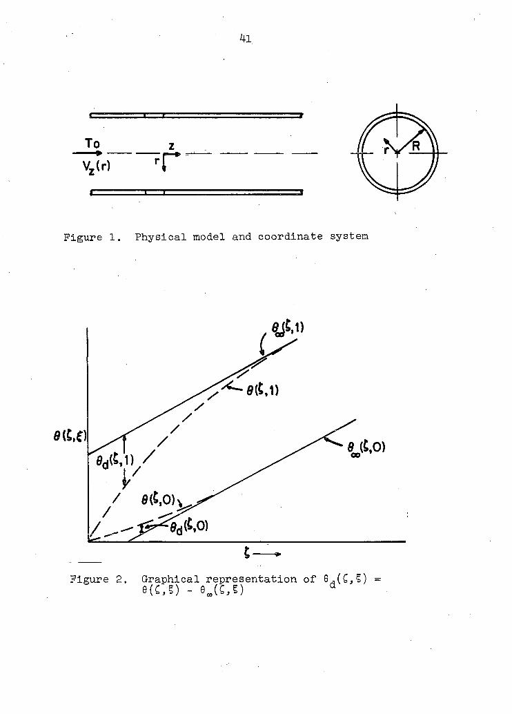
nates and system geometry are shown in Figure 1. For

z < 0, the fluid temperature is uniform at Tq; for z > 0,

there is a prescribed wall boundary condition. It is de­

sired to determine the thermal distribution and the varia­

tion of important heat transfer parameters. For the

present, viscous dissipation and uniform heat generation

will be neglected; however, later in the analysis, the in­

clusion of these terms will be discussed. Essentially

four models will be treated, i.e., constant wall heat flux

or constant wall temperature with either plug flow or

fully-developed laminar flow.

Model I. Constant wall heat flux - plug flow

Using Equations 23 and 28, the boundary value problem

may be described mathematically by the following partial

differential equation and boundary conditions.

= (Eq. 60)

41

To —» -Vz(r)

Figure 1. Physical model and coordinate system

1) /

i

Figure 2. Graphical representation of 6,(G,§) = e(c,s) - 9.(c,5) d

r

42

B. C. 1. at r = 0 T = finite (Eq. 6l)

B. C. 2. at r = R k = q^ (constant) (Eq. 62)

B. C. 3. at z = 0 T = Tq (for all r) (Eq. 63)

To simplify manipulations, the following dimensionless

quantities will be used.

T - T 0 = (Eq. 64)

q^R/k

§ = r/R (Eq. 65)

e = (Eq. 66) PC V R Pe Pe' P Z

The equation for thermal distribution then becomes

i£ = (çli) + 1 l£§ (Eq. 67) aG S as as pe'^

with boundary conditions

B . C . I , a t § = 0 © = f i n i t e ( E q . 6 8 )

B. C. 2. at § = 1 — = 1 (Eq. 69)

B. C. 3. at G = 0 8 = 0 (Eq. ?0)

43

When the wall heat flux Is constant, it Is known that for

very large values of G there is a fully-developed or

asymptotic thermal situation which is characterized by the

following temperature distribution (see Appendix).

,(G,§) = 2G + 1

8 (Eq. 71)

In addition to satisfying the conservation of energy,

Equation 71 includes the following conditions :

38.

3C = constant,

a§

38 = 0,

5=0 3§ = 1 (Eq. 72)

5=1

The thermal distribution in the thermal entrance region

can be obtained by using a difference function, 9 d ( G, 5 ),

defined as

Gd(G,5) = 8(G,S) - 8jG,5) (1%. 73)

where 6(G,5) is the true thermal distribution. A graphical

representation of Equation 73 is given in Figure 2. The

difference function may be considered to be the difference

between fully-developed heat transport and the heat trans­

port that is actually present. This method of superposi­

tion has been used by Siegel _et al. (65) and Labuntsov (40)

for similar problems. Substitution of 6(G,5 ) from

44

Equation 73 into Equation 67 yields a system which 6^(C,§)

must satisfy.

ffd = 1 a _ ( S ffd) + -JL_^ (Eq. 74) dC § a§ d§ p e

1 dC^

B. C. 1. at C = 0 ed = - eœ = - §2 + ± (Eq. 75) 8

B. C. 2. at § = 0 8^ = finite (Eq. 76)

B. C. 3. at S = 1 d6d/d§ = 0 (Eq. 77)

B. C. 4. limit 0d = e (Eq. 78)

Before proceeding to a formal solution, a few general

observations may help to clarify the mathematics. Because

of the nature of the boundary conditions and previous

knowledge of heat transport problems in cylindrical

geometry, one intuitively would expect the solution for

6d(C,5) to consist of Bessel functions in combination with

exponential functions. The classical method of separation

of variables applies directly to the problem; however, if

a solution is assumed of the form exp(XC) i|f(§), Equation

74 reduces to

+ 1 M + - Xlt = 0 (Eq. 79) d§ § d§ Pe'

45

which may be written as

+ 1 âî + a2t[f = 0 (a real) (Eq. 8o)

dr : a§

The eigenfunctions of Equation 80 are Bessel functions of

zero order, and the characteristic values, a, and the

eigenvalues, X, may be determined from the boundary condi­

tions. Although this is a simple example, it may be con­

sidered in connection with the theory presented in the

previous section, and Equation 4l is the auxiliary equation

with Equation 80 corresponding to Equation 46.

In order to allow a more general solution, let

00 Z (G)J (a §) 8d(C,5) - £ m 0 m (Eq. 81)

Jo(am>

where the functions Z (G) are to be determined from the m

boundary conditions. The characteristic values am are

taken to be the roots of J^(x) = roots of -J^(x) = 0

because of the boundary condition specified by Equation 77.

Substitution of Equation 8l into Equation 74 gives

: z;'£)W> :

m=l j2(am)Pe'2 m=l m=l

(Eq. 82)

46

Multiplying Equation 82 by §JQ(an§), where a need not be

the same characteristic value as a^, and integrating from

0 to 1 using the relations given by Equations 44, 45, and

59 yields

' (Bs- 83) Pe1

This integration procedure is identical to taking the

finite Hankel transform (68) of Equation 82 subject to the

condition (°^) ~ ~^l am^ = ^'

Because the characteristic values, a , are taken to

be the roots of J^(x) and the expansion required to satisfy

the inlet condition (Equation 75) is a Dini expansion (13,

72), it is necessary to include the first root of J^(x),

i.e., 0,^ = 0. Equation 83 will satisfy the boundary con­

dition of Equation 78 if Z (G) = a exp(X G) and Z = a. = e, ill 111 111 -L -L

Evaluating Equation 83 with Z^(G) = a exp(X G) gives

X2 m X _ a2 = 0 (m = 2, 3, 4, ) (Eq. 84)

pe,2 m m

and the mth eigenvalue is taken as the negative root of

Equation 84.

The expansion coefficients, a , may be determined by

the, Fourier-Bessel (Dini's) expansion technique (8, 13)

using the boundary condition given by Equation 75.

47

^ VxP(Xme)'VamS>

m=l

' Î2 i "5 + - (Eq. 85)

c-o 2 8

Taking the finite Hankel transform of both sides of Equa­

tion 85 gives

a i = - f

- 2W>

a ^ ^ r

(Eq. 86)

Then

-, 00 2exp(X Ç )

j 2 ^ f r W ) ( E q - 8 7 ) m 0x iir

and

p2 -, 00 2exp ( X C ) 6 (C , § ) = 2C 4 — - Z —p (am^^

2 4 -2 a2J0(am)

The mixed-mean temperature weighted with respect to

the fluid velocity is defined by Equation 89 (5).

rf I? V -T rdrd6 (Eq. 89)

Jo XS vz rdrde

48

Evaluating Equation 89 using dimensionless quantities and

Equations 23 and 88 gives

^ e(c,5)d§ 0 m ( O ° V sis = g£ (Eq. 90)

The local Nusselt number is defined as

h-, (z ) «D NuloCi(z) = -1°°- (Eq. 91)

where tu (z), the local film heat transfer coefficient, l o c 3

is defined as

hloc*(Z) [T(z,R) - Tm(z)] (Eq* 92)

for heating conditions. Substituting Equation 92 into

Equation 91 and putting the temperatures and independent

variables into dimensionless form gives as the final ex­

pression for the local Nusselt number

• .(J - y » <M'S3>

Evaluating Equation 93 using Equations 87 and 90 yields

Nuloc.'£) °> 2exp(X C) (Eq. 94) •i - E „m

4 m=2 ' am

49

When Equation 94 is evaluated in the limit as Q approaches

infinity, the local Nusselt number approaches 8.0, which

is the value for fully-developed heat transport.

Another heat transfer parameter of importance is the

thermal entrance region, which is defined here as the

axial distance from the entrance to the heated section

necessary for the local Nusselt number to approach within

5 percent of the fully-developed value. The criterion of

5 percent of Nuœ is arbitrary; however, a lower percentage

is not appropriate for engineering work.

The important heat transfer parameters and thermal

profiles may be calculated using Equations 88, 89, and 94.

Model II. Constant wall heat flux - fully-developed laminar flow

The physical description of this heat transport model

is essentially the same as Model I except that the velocity

distribution is fully-developed as given by Equation 24.

The boundary value problem to be solved is given by Equa­

tion 95 subject to the boundary conditions of Equations 61,

62, and 63.

2PC V E l - (r/R)2] = kC^ — (r —) +-^|] P = r &r

(Eq. 95)

50

B. C. 1. at r = 0 T = finite (Eq. 6l)

B. C. 2. at r = R R -g-p = q^ (constant) (Eq. 62)

B. C. 3. at z = 0 T = Tq (for all r) (Eq. 63)

Using the dimensionless quantities given by Equations 64,

65, and 66, the above system reduces to

2(1 „ ;2, = (5 36, + l!| (Eq. 96) 5Ç S 3§ dÇ Pe' dC

subject to the boundary conditions

B. C.l. at § = 0 8 = finite (Eq. 68)

B. C. 2. at § = 1 — = 1 (Eq. 69) as

B. C. 3. at C = 0 0=0 (Eq. 70)

As in Model I, it is known that for large values of Q,

there is a fully-developed thermal situation which is

characterized by the following temperature distribution

(5 , 21 ) .

(^ * ) = 2C + - —- (Eq. 97) 4 24

which satisfies the conditions

51

00 = constant 0 1 (Eq. 72)

Applying the superposition method, let

Gd(C,S) = G(G,5) - 8JG,S) (Eq. 73)

where 0(C,§) Is the true thermal distribution as shown in

Figure Û.

When Pe' is large, the contribution of the last term

of Equation 96 is negligible and this limiting case has

been worked out by Siegel et al. (65) . In the presentation

here, Pe1 is a parameter which may or may not be large.

Evaluating Equation 96 with Equation 73 yields a sys­

tem for 6d(Ç,S) .

aG 5 as as (Eq. 97)

B. C. 1. at C = 0 9 = -em = -I2 + J_ + -I (Eq. 98) a 4 24

B. C. 2. at § = 0 G = finite

ô6d B.,C. 3. at 5 = 1 —- = 0 d§

(Eq. 76)

(Eq. 77)

B. C. 4. limit 0d = e (Eq: 78)

52

From the analysis of Model I and the above boundary

conditions, it is anticipated that Bessel functions and

exponentials will be characteristics of the solution for

9d(Ç,§). Indeed, if the expression 9^(C,§) = exp(XC)H ?)

is substituted into Equation 97, a generalized Sturm-

Liouville equation is obtained.

A_| + 2 ÛÏ + [_L_ _ 2X(1 - §2)]i|/ = 0 (Eq. 99) d§ § d§ Pe'

Applying the theory presented in the previous section, the

auxiliary equation may be taken as Bessel's equation of

zero order and the eigenfunction, t|/ ( § ), may be expressed

as a series of Bessel functions of order zero.

CO

*(§) = z C J (a S) (Eq. 100) p=l P ° &

The characteristics values, a , are chosen to satisfy

the condition i|/1 ( 1 ) = 0. This corresponds to the second

form of the special boundary conditions represented by

Equation 59, and therefore, the characteristic values are

the zeros of J'(x)=roots of J,(x). Because the eigenfunc­

tion expansion given by Equation 100 in combination with

the special boundary conditions is a Dini expansion (13,

72), it is necessary to include the first root of J^(x),

i.e., 0 •

53

At this point of the development, an expansion of

8^(£,§) could be assumed as in the treatment of Model I.

However, it is better to apply the theory as presented in

the mathematical development section directly. Using

Equations 46, 47, 53, 54, 99 and 100 with q(x) = 0,

v2/x = 0, and g(x,X) = SE ^ g - 2X(1 - S2)], and the fol­

lowing correspondence : x = 5, U^(x) = J0(am )* X(x) = $(§),

C = C , a = 0, and b = 1, the equations below define the m nr ' ^

elements of the system given by Equation 52.

Amn - V - /o - ad - e2)]J0(V)Jo<Vs)a5

(Eq. 101)

V - ' a"Jg°(am) + To - 2 -

(Eq. 102)

Using the orthogonality relations of Equations 44, 45, and

59 gives

\n = Anm = 2X To 103)

A™ - [ 72 * 2X - »m] 7^ + 2X £ 53jo(%5'd?

(Eq. 104)

The remaining integral for A^ can be evaluated by using

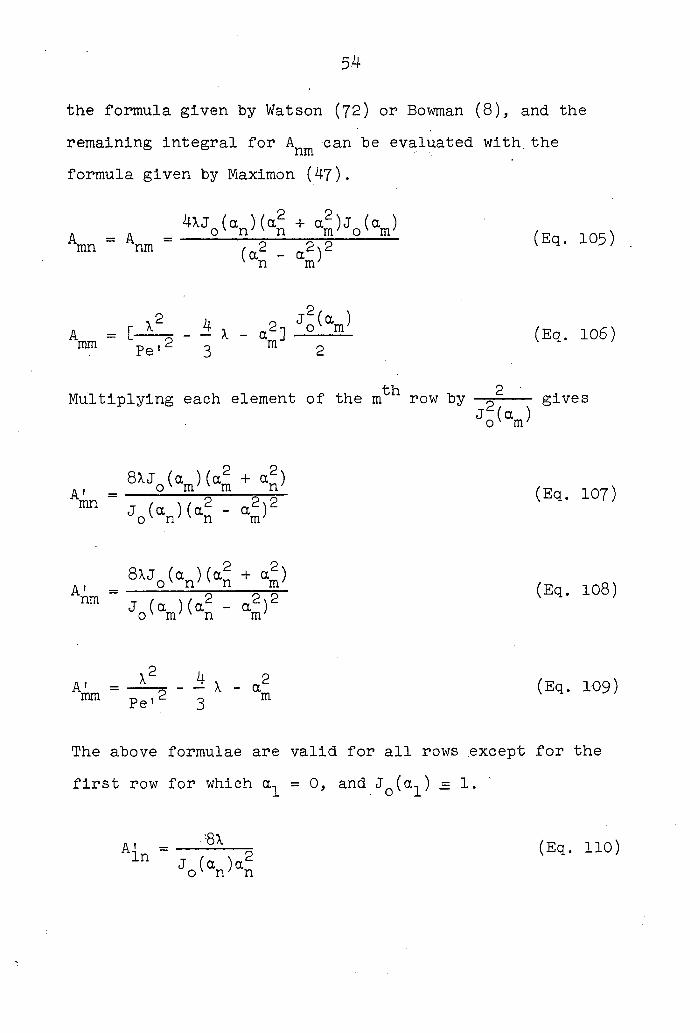
54

the formula given by Watson (72) or Bowman (8), and the

remaining integral for Anm can be evaluated with, the

formula given by Maximon (47).

V - V - 4U°(aff" (Eq. 105)

v • • 3x " a™] 4^ (Eq-106}

th 2 Multiplying each element of the m row by —5 gives Jo<am>

^ " 4 (»«• l°9>

The above formulae are valid for all rows except for the

first row for which = 0, and JQ(a^) = 1.

55

\2 A' = p - X (Eq. Ill) 11 Pe'

Hence, the infinite system of algebraic equations for the

determination of the associated coefficients, Cn, may be

represented by

œ 8XJ ( cc ) ( a2 + a2) f(X,n)C + Z ° ? 2\- Cr/P " M %) = 0

p=l J0(ap)(a2 - an) P (Eq. 112)

8XC f (X, 1 )C, + s E_^ = 0 (Eq. 113)

p=2 J0(a )(a^)

where

2 f(X,n) = - - X - a2 (n = 2, 3, 4, ) (Eq. 114)

Pe1 3

and

y 2 f(X, 1 ) = - X (Eq. 115)

Pe'

In order to obtain a non-trivial solution to the above . :

set of homogeneous equations, the determinant of the co­

efficient matrix must equal zero and the system must sat­

isfy the convergence requirements. It is obvious that

X = 0 is an eigenvalue because all the elements of the

56

first equation are then zero. However, in such a case,

the elements of the Infinite system could not be derived

by any means because the integral of the generalized

Sturm-Liouville equation is identically equal to zero and

^(Ç) = a constant = C^(l). Any difficulty which this may

give toward convergence may be remedied by assuming that

only for eigenvalues greater than m=l will any algebraic

manipulations be performed. Then the system of equations

yields an infinite number of eigenvalues and the associated

coefficients for the corresponding eigenfunctions. The

system of equations may be written compactly as

(Eq. 116)

and

A' li Pe1 3

2 4 2 — _ — X - (i = 2, 3, 4,

(Eq. 11?)

(Eq. 118) Pe'

subject to the condition

A(X) = ] A«j = 0 (i,j = 1, 2, 3, (Eq. 119)

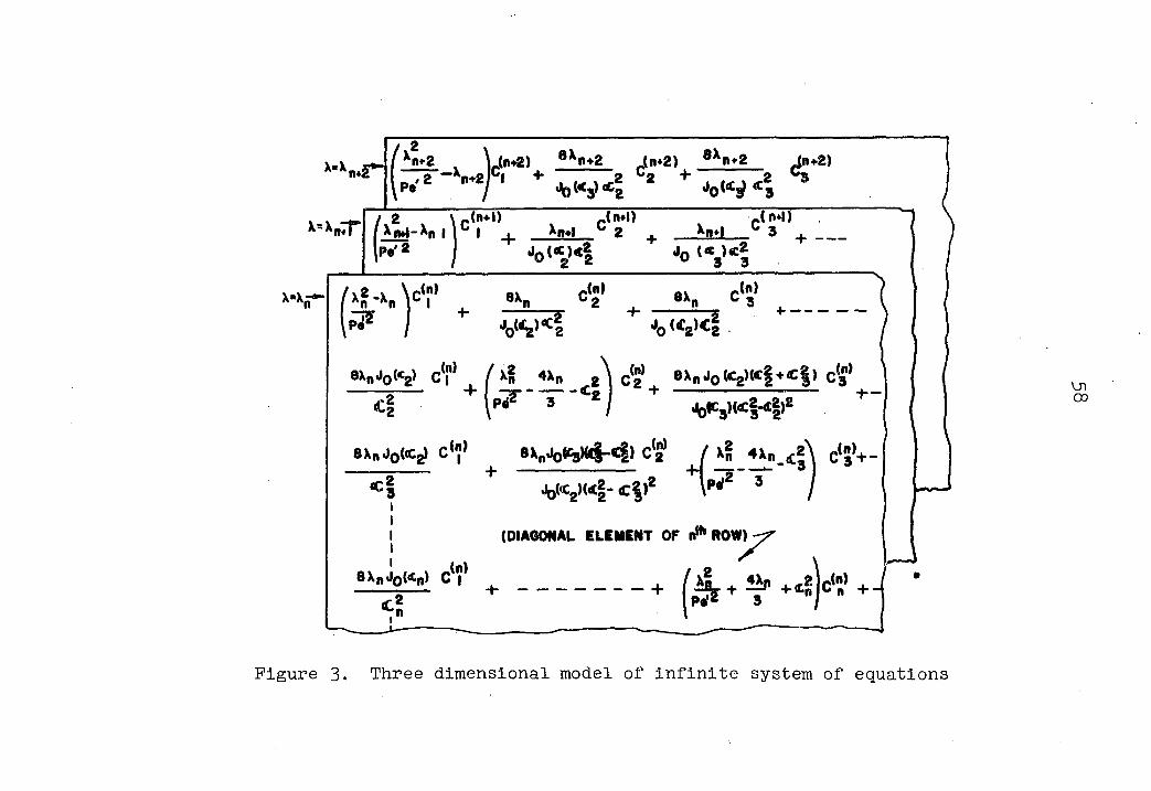
A graphical representation of the system of equations

57

may help to clarify this portion of the solution develop­

ment. For each eigenvalue X , (m = 1, 2, 3, . ..), there

exists a set of associated coefficients (p = 1, 2,

3, ...), which define an eigenfunction as given by

Equation 100. The system of simultaneous algebraic equa­

tions for the eigenvalues and associated coefficients may

be represented by a three dimensional model given by

Figure 3. For each plane of the model there corresponds

an eigenvalue and a set of associated coefficients which

determine the related eigenfunction. Thus, the model for

the equations represents a three dimensional infinite sys­

tem, from which the characteristic parameters must be de­

termined, In a sense this problem is mathematically simi­

lar to the plug flow problem of Model I for which only the

diagonal elements of the infinite system are present as

given by Equation 84.

In order to calculate the associated coefficients and

eigenvalues, the m^ coefficient of the m^ eigenvalue,

C^, may be set arbitrarily equal to unity because the

proper scaling may be done in the determination of the ex­

pansion coefficients to satisfy the condition prescribed

by Equation 98. In the case of ^ = 0, is unity and

the remaining coefficients are identically equal to zero.

For m = 2, the following iterative procedure may be used

to calculate the eigenvalue, X , and the set of associated

X"Xm2*"

x=xn7T

/ 2 Xn»2 \ Jtn+2) eXn*2 Jn*2) 8Xn*2 (n+2)

Pe'2 y 1 + 4O«3>4 2 + J0<S4 3

(, 2 \ q("*0

xn*l xm4-xn I I I i P.* 2 1 JqCCXI

,( n»l) x«*»

»( n4)

J0 «e,,e| +

ex. Jm) 8X„ ,(n)

J0(C2)C|

8Xn«f()(*2 Clf ( X$ 4Xn g\ çfë 8XnjQtogXcl + C^)

<C| [pT"T ' C z j + W(<C| |,2

8XnJqCC^I C<»> *K<b*M-4) C(2 Z xn 4 X n (C2\ c^-h-

• 3 I I I I I

Z xn 4Xn (r7"T

W4- cl'2

(DIAGONAL ELEMENT OF i * ROW)

.2 %

c<î' + + + -+tsjc«?+-

Figure 3. Three dimensional model of infinite system of equations

59

coefficients, . Initially, the eigenvalue may be

approximated as the negative root of the diagonal element,

i.e., f(X ,m) = 0, and then the coefficients may be approx­

imated by using only the m**1 term of the ntla equation,

•-'$5 -* c ( m ) ~ V o ' " » ' ( E q . 1 2 1 )

1 4 • '(v1)

Using the estimates for the coefficients, the summation

t h term for the m equation may be calculated.

Sum - È 8j°(V)(gm + "p^p"' (p m) (Eq. 122) p=l J0(ap)(a2 -

Then a new estimate for the eigenvalue may be calculated

using

— + Sum -!/(-- Sum)2 + —^

^ Pe'

Using their respective equations, the associated coeffi­

cients are then recalculated with the new value of X m

(except for which is assigned the value of unity).

The iterative procedure of computation of the eigen­

value and the coefficients may be repeated until the

60

desired accuracy is attained. The above calculation

method is a modified Gauss-Seidel iteration (27, 43) to

calculate coefficients for a homogenous system of equa­

tions.

The constants of integration or expansion coefficients,

a , must be determined because thus far they have been

chosen arbitrarily by setting = 1.0. The inlet con­

dition at G = 0 is prescribed by Equation 98,

Gd(G'5)lG=o = - 8.(G,§)|g^o = - + 1_ + _Z (Eq. 98)

which may be written as

where

= Ç C^)jo(o.p§) (Eq. 125) p—1

Taking the finite Hankel transform of Equation 124 on the

interval (0,1) using the formulae given by Bowman (8) gives

2

2 ^ C<m)J (g ) = (an4+ 8) (n 2 2) (Eq. 126) m=l J*(aJ " o n 4

f + 1: + _z 4 24

(Eq. 124)

6l

and

£ g 1 = - — (n = 1) (Eq. 127) m=l J0(am) 16

This system provides an Infinite set of simultaneous equa­

tions for the calculation of the am's. However, according

to Dennis and Foots (15), these are unsatisfactory gener­

ally for computational purposes due to the slow convergence

and it is better to proceed as follows. Using the varia­

tional principle that the quantities am must be chosen so

that when Ç = 0, the integral

, 00 2a /f I(ava2, an ) = t E „ ^(5)

m=1 o m'

+ (g2 _ 1^ _ _Z)/g]2d§ 4 24

(Eq. 128)

shall achieve a minimal value. From the theory of the

calculus, for a function F = F(x^, x2, x^, ....xn....) to

ÔF achieve a minimal value, it is necessary that 3— (x, , x0, xn

....x ....) = 0; therefore,

k'(ai"-a"---) = 2j,°c„fi *»(s) + (?2 • f" • i)/I] ox rir

n d§ = 0 Jo<an>

62

Integration yields

I l ç (m)ç (n) J^(q )] -fi!! . Ë Cpn)jO(V(ap + 8>

m=l j2(Ga) P=1 P 9 ° P 16 p=2 *4

(n : 2) (Eq . 130 )

and

05 a„C-(m)

Z — = for n = 1 (Eq. 131) m=l JQ(am) l6

Although the above equations are more complicated, the

derivation of the expansion coefficients from them is more

accurate.

The final solution may be represented by

B(c,s).2c + !2-i?-4- l 2Yxp("mC) •.(«) 4 24 m=l J^(am)

(Eq. 132)

where tym(§) is given by Equation 125. Using Equation 89,

the mixed-mean dimensionless temperature for fully-

developed laminar flow is

5(1 - S g )8 (C ,S )dS

~ ^ 1(1 - 5 2 )d5 6 „ ( C ) = " 1 _ 0 . . (Eq . 133 )

' O

Integration of Equation 133 using the value for 0(C,§)

63

given by Equation 132 gives

00 2a exp(X £ ) » C^J (a ) 6 (C)= 2C+8 Z—SL E_ [ E _E °—£_] (Eq. 134)

m=l p=2 a;

Applying the definition of the local Nusselt number

(Equations 91, 92 and 93) yields

NUl0C-(c) ii : yxp(V) f %(%)( +

48 m=2 j2(a^) p=2

(Eq. 135)

It should be noted that for fully-developed heat transport,

Nuœ = 48/11 = 4.364. Evaluating Equation 135 in the limit

gives

limit NU1qc (C) = 48/11 = 4.364 (Eq. 136)

Ç - * oo

An approximate solution may be obtained by setting

tm(§) = J0(am ) and the eigenvalues are the negative roots

of the diagonal elements,

X = C — -\ — + —^0 1 Pe12 (m = 2, 3, 4, ...) (Eq. 137) m 3 V 9 Pe1

and X^ = 0. The expansion coefficients may be calculated

from

64

ax = - 1/16 (Eq. 138)

(«S + 8) am = - J0(am) 4 (m = 2, 3, 4, ...) (Eq. 139)

am

Then,

, » 2a2 + 16 1 tv m e d (C,?) = - i - z -zf -—: e x P(V ) J o ( % 5 ) < E < 3- i4o) 8 m=2 a^J0(aJ

and

etc,5) = 2C + + L. - -5 ^ 5^ exp(XmC)J0(am5)

m ov my

(Eq. l4l)

Again applying the definitions of mixed-mean temperature

and Nusselt number, the following equations are obtained.

, » a2 + 8 0(C) = 2C - 2 + 16 S m exp(XC) (Eq. 142) m . 8 m=2 a6 m

m

48 m=2 m m

Model III. Constant wall temperature - plug flow

This problem is essentially the same as Model I ex­

cept that the wall boundary condition is constant wall

65

temperature. It may be described by the equations

PC VZ IT = K[L D_ (r ÔTj + l^T] (Eq. 60) p dz r dr dr dz

B.C. 1. at r = O T = finite (Eq. 6l)

B. C. 2. at r = R T = (for z > 0) (Eq. 144)

B.C. 3. at z = O T = Tq (for all r) (Eq. 63)

B. C. 4. limit T = Tw (Eq. 145)

Using a dimensionless temperature

T - T w

To - Tw

(Eq. 146)

and the quantities £ and § defined by Equations 65 and 66 ,

the system becomes

+ 1 (Eq. 67) ac ? 55 a? Pe'2 3C

B. C. 1. at § = 0 0= finite (Eq. 68)

B. C. 2. at 5 = 1 0=0. (for C > 0) (Eq. 70)

B. C. 3. at C =0 0=1 (for all S) (Eq. 14?)

66

B. C. 4. limit 9=0 (Eq. 148)

Ç - * 00

The solution to the above problem may be written as

where a is a positive root of J (x) because of Equation m o

70. Substituting the expansion into Equation 134 and

taking the finite Hankel transform on the interval 0 to 1

gives

Again, two values of X are possible; however, only the

negative root is admissible because of the boundary condi­

tion specified by Equation 148.

The expansion coefficients, a , are determined using

Fourier-Bessel expansion theory subject to the condition

given by Equation 147.

(Eq. 149)

a. 'm (Eq. 151)

The mean-mixed dimensionless temperature for plug

flow is obtained by use of Equation 89.

67

en(-C).V£LJÏ-_ - WV1 (Eq. 15„ To - Tw »-l am

The local Nusselt number is determined using Equations am

91 and 92 with q = - k -gp r=R

. 2R

"u, (z) -£-S (Eq. 153) Tm<z> - Tw

Applying the definitions of C, §, and 6(Ç,§) from Equations

65, 66, and 146 yields

CO

E exp(Xm^)

loc.(0 - "Z1 expix i) (Eq. 154) s JH— m=l a2

This problem has been considered in detail by

Schneider (63) and Singh (67); however, the important heat

transport quantity, the Q ratio, was not calculated.

Because' of the manner in which the local Nusselt num­

ber is defined, it is not constant in the entrance region

and asymptotically approached infinity as Ç approaches

zero. From the standpoint of estimating heat transport,

the conventional method used in forced convection is de­

termination of the local heat transfer coefficient followed

by calculation of the total heat transport. This extra

68

calculation may be eliminated in certain cases, and in

particular, the total heat transport may be calculated

directly from the analytical solution for constant wall

temperature problems. For the models associated with the

boundary condition of constant wall heat flux, the calcu­

lation of total heat transport is trivial because it is

specified as the wall boundary condition. However, because

physical systems do not follow either wall condition ex­

actly, the analysis of both conditions is advantageous.

To calculate the total heat transport, the first law

of thermodynamics in integrated form may be applied to an

open system giving

Q(G) =ÂH(£) = pVzSGp[Tm (C) - To] (Eq. 155)

2 where S = nR = cross-sectional area of tube. Equation

155 states that the total heat transport equals the product

of mass flow rate times the mean change of enthalpy of the

fluid. After rearranging, the equation becomes

Q(C) [T (0 „ T ] (Eq. 156) 2-R m °

Then using the definition of 8^(C) given by Equation 152

and a few algebraic manipulations, the above equation

reduces to

69

Q-ratio âliJ = - Cl - 0 (C) ] (Eq. 157) Pe-k.2R[T - T ] 4 m

w o

Therefore, by using Equation 157, the total heat transport,

~Q(C), may be calculated if the fluid properties, tube

radius, and the inlet and wall temperatures are known. The

utilization of the Q-ratio eliminates the ambiguity of the

non-constancy of the heat transfer coefficient in the

entrance region and provides the total heat transport

directly with essentially no intermediate calculation. The

results are general and apply to all fluids which meet the

assumptions made in the analysis. The use of the Q ratio

may be extended to analogous mass transport problems.

Model IV. Constant wall temperature -fully-developed laminar flow

This problem is essentially the same as Model III ex­

cept the fully-developed velocity profile is inserted into

the energy equation.

2pC TCl - (r/R)2] = kC- — (r —) + -^| (Eq. 95) P % r 3r 3r

B. C. 1. at r = 0 T = finite (Eq. 6l)

B. C. 2. at r = R T = Tw (for z > 0) (Eq. 143)

70

B,. C. 3. at z = 0 T = T (for ail r) (Eq. 144) o

B. C. 4. limit T = Tw (Eq. 145)

Substitution of the dimensionless quantities given by

Equations 65, 66, and 146 into the above system gives

2(1 - s2) — = i — (5 li) + -i-5 ih (Eq. 96) ac 5 as as Pe1-2

subject to the conditions

B. C . l . a t § = 0 0= finite (Eq. 68)

B. C, 2. at § = 1 0=0 (for G > 0) (Eq. 70)

B. C. 3. at C = 0 0=1 (for all I) (Eq. l47)

B. C. 4. limit 0=0 (Eq. 148)

This problem has been considered by Millsaps and

Pohlhausen (50), Singh (67), and Abramowitz _et _al. (2),

but none of the important heat transfer parameters have

been calculated except for large Peclet values.

The analysis of this model is a duplicate of the

presentation given by Singh; therefore, the intermediate

71

steps will be omitted. The method of solution is similar

to that used for Model II with constant wall heat flux and

fully-developed laminar flow.

Analogous to the pattern shown by the previous models,

let

" 2ZJO 8(C,S) = Z -g2 Jn(am5) (Eq. 158)

m=l JX>

Substituting the expansion for 0(C,§) into Equation 96

followed by taking the finite Hankel transform on the in­

terval (0,1) using Equations 44, 45 and 56 gives

S - i(1 - "i. °

(n m) (Eq. 159)

As in Model III, the characteristic values, a , are taken

,to be the zeros of J (x). This system of linear differen­

tial equations will be satisfied by

^ ( C ) = C^exp(XG)

if

l6\a 00 a J, (a, )C^

(Eq. 160)

= 0 (Eq. l6l)

72

where

2 F(X,m) = —~L—p - — (l + -^p)X - cc/~ (Eq. 162)

Pe'^ 3 *

and X is obtained from the condition for non-trivial Cm.

This condition may be written compactly as

A(X) =

where

Ah = 0 (l,j = 1, 2, 3, ...) (Eq. 119)

AijJl<ai> = AjiJl(a3) ° (1 * 3)

(Eq. 163)

and

2 Ai . = o ~ + "~p)X - o3 (Eq. 164) 11 Pe'd 3 ct£ 1

The roots of the infinite determinant define and infinite

number of eigenvalues, and the computational procedure for

the simultaneous calculation of an eigenvalue and its set

of associated coefficients is equivalent to the method

employed for Model II.

To calculate the expansion coefficients, a^, use is

made of the variational principle that the a^ are to be

determined such that when C = 0, the integral

73

,lr : /S I(a ,ag...a ...) = % "if—T - 5 ] (Eq. 165)

m=l Jf am m 1 m

shall achieve a minimal value. Differentiation with re­

spect to am followed by integration gives a set of simul­

taneous equations for the calculation of the expansion

coefficients.

00 a„ œ o 00 ) m Z ci m ' c ln'j?{a„) = S -E 11^1 (nth equation)

(Eq. 166)

m=l j2(am) p=l P P 1 P- p=i ap

The final result for- 6 (C, S) is expressed by Equation

167

" 2am 6(G,5) = Z p ^ exp(X (5) (Eq. 167)

m=l jZ(a^)

where

>m(5) = E c'm)J0(»p5) (Eq. 125) P—1

Use of Equations 133, 146, and 153 with Equation 167 gives

the equations for the calculation of the important heat

transfer parameters.

74

m (0 - T™(c) 'T™

To - Tw

CO £

m=l

32amexP'XmC) (Eq. 168)

nu -(c> - . —. Jl(. >., (Eq-i69)

ml 8a™eXP(X™£) Cpfl ]

Q-ratlo = ^ = — [1 - 0_(C )•] (Eq. 157 Pe-k.2R(Tw - T ) 4 m

Associated Heat or Mass Transfer Problems

In the treatments of the four heat transfer models

the effects of uniform heat generation and viscous dissipa­

tion were neglected. The solutions given for the constant

wall temperature models required that 8(£,§) approach zero

as zeta approaches infinity. When the uniform heat genera­

tion and viscous dissipation terms are included, the

following requirements must-be added (67):

1. Constant wall temperature - plug flow

2 2 a. B. C. 4' as , 6(C,§) - J1 ~ ^ j

° " (Eq. 170)

75

b. a = [1 - , Qr2 ] (Eq. 171) amk<To ' V

e. e(C.ï)- ; + aR2(l - Sg) m-1 Ji(am) tk(T0 - 1„)

(Eq. 172)

2. Constant wall temperature - fully-developed

laminar flow

a. B. C. 4' as C-"„ 8(G,§) - aR t1 ' ? ) 4k(To " Tw>

(Eq. 173)

_ ^ ( l - i 2 )

+ k<To - T„>

b. £ g3*1 E Cim'Cnn^Jl(an' = m=l J^(am) p=l P P 1 P

: 4n)W ; c p n ) j i ( % ) r g r 2 S —E V-El - Z -E |l-Ei [

P-l <xp P=1 ap k(T0 - Tw)

UV? , + (1 ô) 1 n-th equation

k<To - T„> % (Eq. 174)

76

+ GR2(i - g2)

4k(To - T )

(Eq. 175)

+

The eigenvalues, X , do not change; however, the values of

the expansion coefficients change accordingly as given by

Equations 171 and 174.

The constant wall heat flux models may be treated in

a similar manner by including the uniform heat generation

and viscous dissipation terms in the fully-developed heat

transfer solution, 9œ(C,§). These terms are given in

dimensionless coordinates by Equations 176 and 177.

The expansion coefficients for 8^(G,§) will change de­

pending on the numerical values of the parameters in

Equations 176 and 177.

Other forms of the velocity profile as given by

G* = (Eq. 176) q q

(Eq. 177)

77

Equation 178 may be treated in the same manner as the

models which used fully-developed laminar flow.

V = V max. (1 - §n) n = 1, 2/3, (Eq. 178)

The elements of the infinite determinant would change de­

pending on the values of the integrals given by Equations

53 and 5^.

The analogy between heat and mass transport may be

applied directly to the models provided that the mass dif-

fusivity, density, viscosity, and concentration are con­

stant (5). In mass transport, the Peclet number is de­

fined as Pem = 2RVz/^, where <& is the mass diffusivity.

The magnitude of for most fluids is 10~^ to 10"^ ft2/hr.

Therefore, the Peclet number for mass transport usually

will be 100 or greater, and the analyses which neglect

axial diffusion generally will be valid. If the Peclet

number is small, the results of this work would apply.

Constant wall mass flux does not correspond to any

physical situation although such a boundary condition may

be approximated possibly by the uniform passage of material

through a fine sieve-type wall.. A mass transport problem

analogous to Models III and IV (constant wall temperature)

would be a fluid flowing in a tube with material at the

wall diffusing into the moving fluid. This situation is

78

met in the analysis of mass transfer to the upward-moving

gas stream in wetted-wall-tower experiments (4). Another

case would be steady isothermal flow of a liquid solution

of A and B in a tube whose wall is coated with a solid

solution of A and B, which dissolves slowly and maintains

a uniform liquid composition along the dissolving surface

(5). The total mass transport for either plug flow or

fully-developed laminar flow may be determined from the

Q-ratio (Equation 157) "by substituting Pe^ for Pe, for

k, and C for T and using Equations 152 and 168, respec­

tively.

Mass transfer problems with an accompanying chemical

reaction as discussed by Lapidus (42) may be analyzed by

the methods employed on the heat transfer problems. The

method would apply directly to those cases for which the

reaction is zero or first order. When the chemical re­

action is second or higher order, a non-linear term would

appear in the system of differential equations and a more

refined treatment would be necessary.

79

RESULTS

Calculations

The roots of J'(x) and the zeros of J (x) as given by

Gray and Mathews (23) were checked by linear interpolation

of the Harvard tables of Bessel functions (26). The values

agreed for eight significant figures. The Bessel functions

of orders zero and one were obtained by using a special

subroutine written by Boessenroth (7). A listing of the

Fortran program for the subroutine is given in Figure 40

in the Appendix.

The computations for the plug flow models provided no

difficulty because the calculations of eigenvalues, eigen-

functions and coefficients do not require iteration. In

both models a total of thirty-two eigenvalues and Besse.l

functions were computed for the series solution. The cal­

culated eigenvalues, and expansion coefficients for the

plug flow models are listed in Figures 42 and 44 in the

Appendix.

For the constant wall heat flux model with fully-

developed laminar flow, the infinite system of homogeneous

algebraic equations was approximated by using the first

thirty-two equations. The eigenvalue-associated coeffi­

cient calculations proceeded with no difficulty for values

80

of Pe1 as large as 10. For Pe1 g 10, a total of 20 eigen­

values and corresponding sets of 32 associated coefficients

were determined and each eigenvalue required a maximum of

five iterations to achieve six place accuracy. When Pe'

was greater than 10, an instability occurred in the itera­

tive method of calculation used to determine the eigen­

values. At Pe' = 20, only six eigenvalues could be calcu­

lated before instability .occurred. For Pe1 > 50, a maximum

of four eigenvalues could be computed without reaching in­

stability. The instability occurred usually at the third

or fourth iteration and the recalculated eigenvalue was

-10^ or less.

According to Hildebrand (27), systems of equations in

which small errors in the coefficients or right-hand mem­

bers may correspond to large errors in the solution are

often said to be ill-conditioned systems. These are char­

acterized by the fact that the determinant of the coeffi­

cient matrix is small, in magnitude, relative to certain of

the cofactors of the elements of the matrix. When such a

system is encountered, either the inherent errors must be

made small by retaining a large number of significant

figures or the fact must be accepted that inaccuracies per­

mit the solution to be determined within relatively wide

error limits. Lapidus (43) gives a number of criteria pro­

posed by various authors to estimate quantitatively the

81

condition of a matrix. Two of these criteria are :

1. The numerical value of the determinant of the

matrix can Tbe used as a condition of a matrix. When the

value is very small, the matrix is ill-conditioned.

2. The P-condition number defined as

is a simple measure. \n is the largest and is the

smallest root of the matrix. When P, is very large, the

matrix is ill-conditioned; when P ~ 1.0, there is little

spread in the roots and the matrix is well conditioned.

Although the above criteria are usually applied to non-

homogenèous systems, they do provide some indication on the

condition of a homogeneous system of equations. The P-

condition number for the system of equations under con­

sideration at Pe' = 100 is approximately 400, but at

Pe1 =10 and Pe1 =1, the P-condition numbers are approxi­

mately 70 and 29, respectively. Although care must be

applied in interpreting the numerical meaning of the P-

condition number, the above information indicates a possi­

ble source of the difficulty. The use of double precision

arithmetic on the digital computer was considered; however,

the computational time increases by a factor of about ten

and many times the final results are no better than when

82

single precision arithmetic is used. Another possible

source of the difficulty is in the extraction of the root

of a quadratic with a subsequent loss of significant

figures. To remedy this calculation error it would be

necessary to use multiple precision arithmetic or check the

root by re-evaluation of the quadratic.

The fact that the determinant of the coefficient

matrix is identically zero for an eigenvalue provides a

direct method of calculation of the eigenvalues. A de­

terminant evaluation program using input eigenvalues was

tested; however, the necessary computational time was quite

high to obtain sufficient points for interpolation. A

graphical interpolation of the results for several eigen­

values was tried, but the resulting four significant fig­

ures could be obtained more easily from a plot of the data

for Pe1 g 10 and the asymptotic eigenvalues given by

Siegel _et al. (65). Even if the eigenvalues were deter­

mined with sufficient accuracy by the determinant method,

the associated coefficients would remain to be calculated.

Because of the difficulty associated with the deter­

mination of the higher eigenvalues for large Pe', the first

four sets of eigenvalues and associated coefficients were

used for Pe' ^ 50. The eigenvalues for n = 5 to n = 8 were

approximated from a plot using the values given by Siegel

et al. (65) for Pe1 > 1000, and the data for Pe1 <10.

83

The corresponding associated coefficients were approximated

by using those determined for Pe' = 10. In all cases, the

expansion coefficients were calculated by using the sub­

routine program MATINV(REVISED) written by Boessenroth (6).

This subroutine program is listed in Figure 4l in the

Appendix. The expansion coefficient calculation was com­

pared by using Equations 130 and 131 which were derived by

the variational method and by using Equations 126 and 127

which were derived by the classical method. The values of

expansion coefficients calculated by the two methods agreed

closely at small values of Pe'. As Pe' was increased, the

variational method provided a set of expansion coefficients

which monotonically decreased in magnitude. The coeffi­

cients calculated by the classical method showed the same

behavior for one-half of the set, but a reversal of the

trend occurred for the second half. It was concluded that

the variational method provided a more accurate set of ex­

pansion coefficients. Listings of programs and the eigen­

values and coefficients are given in Figures 34 and 43 in

the Appendix.

The calculations for the eigenvalues of the constant

wall temperature model with fully-developed laminar flow

exhibited the same type of instability found with Model II.

As a result, the eigenvalues computed by Abramowitz _et al.

(2) were used for Pe' > 5, and the sets of associated

84

coefficients were calculated by a separate program using

the input eigenvalues. The basic theory for the solution

of a homogeneous system of algebraic equations in terms of

one of the unknowns is presented by Hohn (28). For the

system of equations under consideration, with X known and

C^m) = 1.0, the remaining coefficients can be calculated

by standard matrix routines. Again the subroutine

MATINV(REVISED), which uses the Jordan method, was used

in the program. For large Pe', inaccuracies were obtained

in the calculations; therefore, only six eigenvalues were

used for Pe' =50 and Pe' = 500. Only twenty associated

coefficients were used because the higher numbered terms

were not very accurate due to accumulated computational

error. The eigenvalues, coefficients, and the computer

programs used are listed in Figures 45, 37 and 38 in the

Appendix.

Constant Wall Heat Flux Models

The important heat transfer parameters were determined

using the equations derived for Model I (plug flow) and

Model II (fully-developed laminar flow). The calculations

were performed on the IBM-7074 digital computer using the

Fortran source programs listed in Figures 33 and 35 in the

Appendix. The computer output data for the various Pe'

85

values reported are available elsewhere (29, 30).

Model I. Plug flow

The local Nusselt numbers for Model I are presented

In Figure 4 with the dimenslonless axial distance, zeta, as

the independent variable. The curves illustrate the dif­

ference obtained in the value of the local Nusselt number

as Pe1 is varied. When Pe1 > 100, the curves coincide.

The asymptotic Nusselt number for all Pe' is 8.0. The data

are presented in Figure 5 using z/R as the independent

variable, and this provides a better picture of the varia­

tion of Nusselt number with a change in Pe1 or axial dis­

tance. The data for Pe1 = 500 were assumed to represent a

solution for which axial conduction is neglected, and they

were used to calculate the data for the curves for Pe1 =1

and Pe1 =10 with axial conduction neglected. The curves

indicate that when axial conduction is neglected, the

thermal entry length is underestimated. This effect is

negligible for Pe' 50.

Because the wall heat flux is specified for this

model, the neglect of axial conduction should affect the

temperature distribution at the wall. Figures 6, J, and 8

show the dimenslonless wall temperature when axial conduc­

tion is neglected and included for Pe1 = 0.1, 1, and 10,

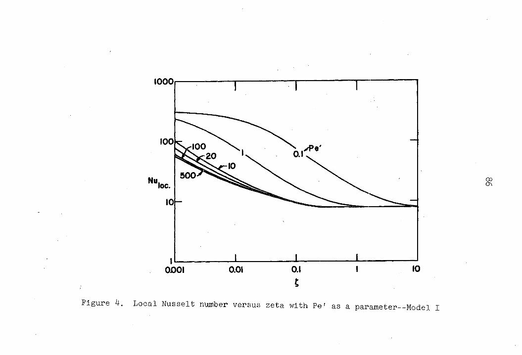
1000

CO CT\

Figure 4. Local Nusselt number versus zeta with Pe' as a parameter—Model I

1000

AXIAL CONDUCTION INCLUDED

AXIAL CONDUCTION NEGLECTED

100 Pe'

100 500;

100 0.01

Figure 5. Variation of local Nusselt number with Pe' and axial dlstance--Model I

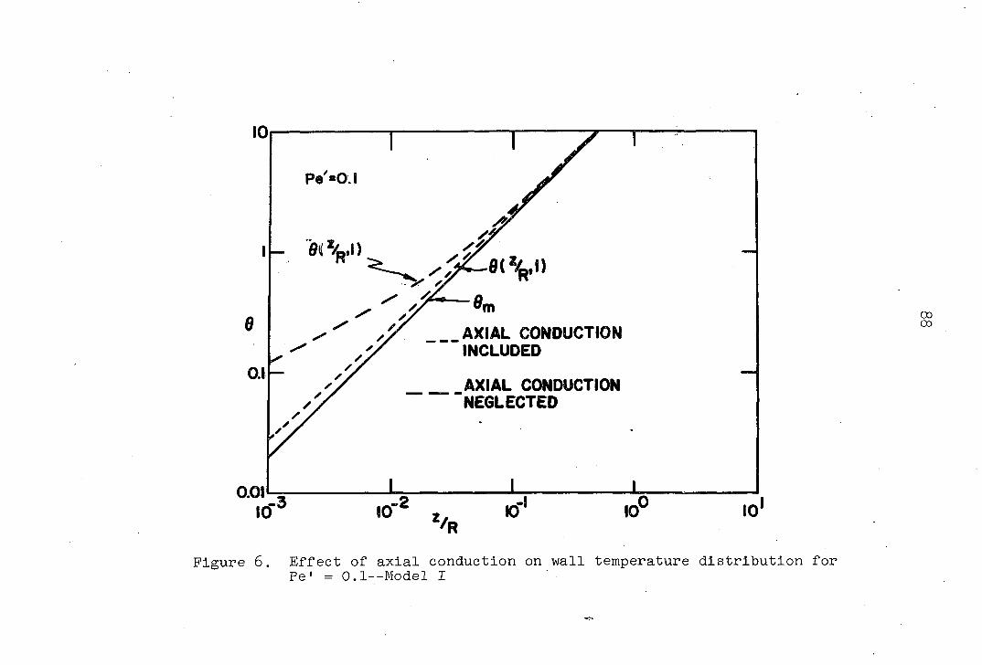
Pe'*O.I

AXIAL CONDUCTION INCLUDED

AXIAL CONDUCTION NEGLECTED

0.01

Figure 6. Effect of axial conduction on wall temperature distribution for Pe1 = 0.1--Model I

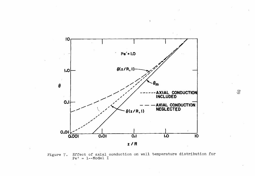
X / AXIAL CONDUCTION / / INCLUDED X /

AXIAL CONDUCTION NEGLECTED

Pe = 1.0

e(z/R,l)

0.01 -0.001 10

CO VÛ

Figure J. Effect of axial conduction on wall temperature distribution for Pe1 = l--Model I

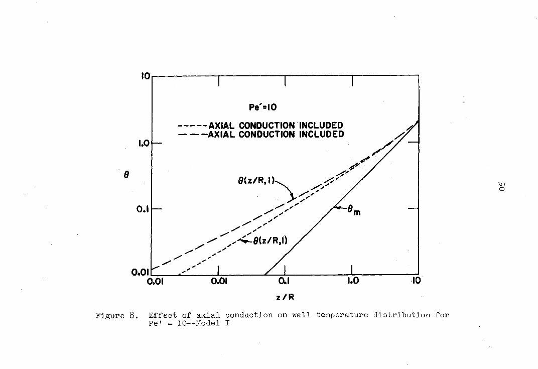
10

Pe'=IO

1.0

Q

0.1 —

0.01

AXIAL CONDUCTION INCLUDED -AXIAL CONDUCTION INCLUDED

0<z/R,l)

0(z/R,l)

10

Figure 8. Effect of axial conduction on wall temperature distribution for Pe1 = 10--Model I

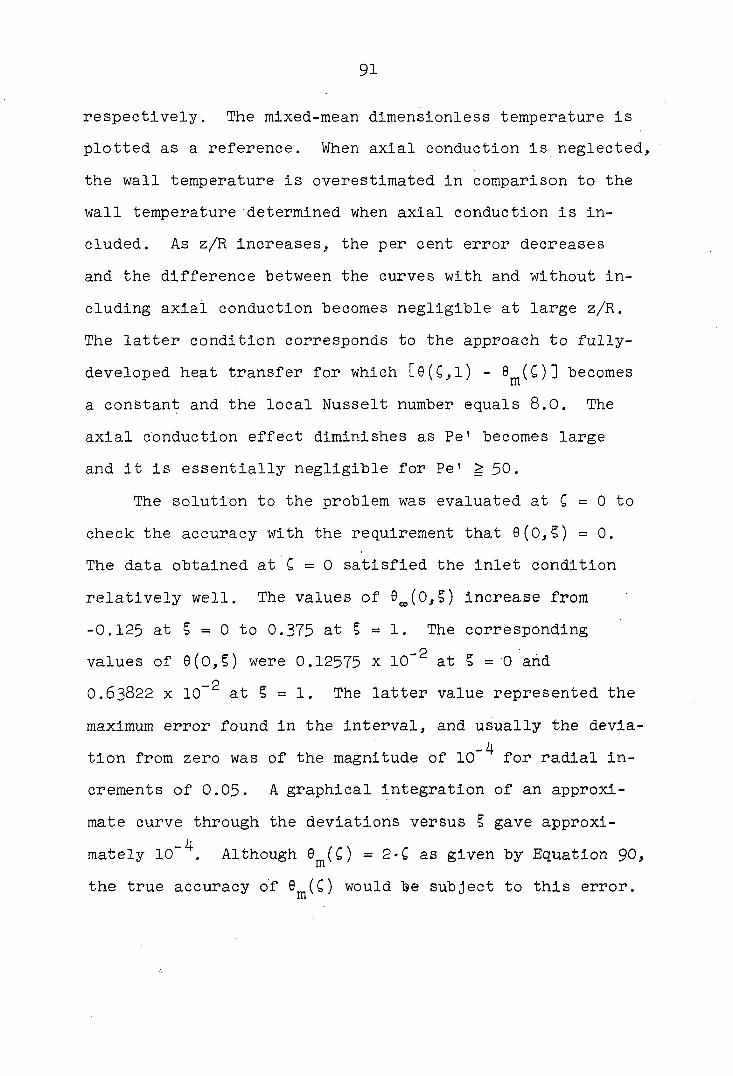
91

respectively. The mixed-mean dimenslonless temperature is

plotted as a reference. When axial conduction is neglected,

the wall temperature is overestimated in comparison to the

wall temperature determined when axial conduction is in­

cluded. As z/R increases, the per cent error decreases

and the difference between the curves with and without in­

cluding axial conduction becomes negligible at large z/R.

The latter condition corresponds to the approach to fully-

developed heat transfer for which C0(C,1) - 8^(G)] becomes

a constant and the local Nusselt number equals 8.0. The

axial conduction effect diminishes as Pe1 becomes large

and it is essentially negligible for Pe1 "t 50.

The solution to the problem was evaluated at C = 0 to

check the accuracy with the requirement that 6(0,§) = 0.

The data obtained at C = 0 satisfied the inlet condition

relatively well. The values of 6œ(0,§) increase from

-0.125 at § = 0 to 0.375 at § =1. The corresponding

values of 0(0,5) were 0.12575 x 10~2 at § = 0 and _ p

0.63822 x 10" at § = 1. The latter value represented the

maximum error found in the interval, and usually the devla-

- 4 tion from zero was of the magnitude of 10 for radial in­

crements of 0.05. A graphical integration of an approxi­

mate curve through the deviations versus § gave approxi­

mately 10"4. Although 6m(C) = 2'C as given by Equation 90,

the true accuracy of ®m(0 would be subject to this error.

92

It can be concluded that the results for the plug flow

model are valid for small values of zeta.

Model II. Fully-developed laminar flow

Values of the local Nusselt number for Model II are

given in Figure 9 with zeta as the independent variable

and Pe1 as the parameter. In Figure 10 the data are

plotted using z/R as the axial variable and the curves

show the influence of the Peclet number on the heat trans­

fer coefficient in the entrance region. The data follow

the same general trend exhibited by the plug flow model.

The effect on the local Nusselt number when axial conduc­

tion is neglected is illustrated in Figure 11 for Pe1 =1.

The neglect of axial conduction would predict a shorter

thermal entry length than when axial conduction is in­

cluded.

The effect produced on the wall temperature by

neglecting axial conduction is given in Figures 12, 13 and

14 for Pe1 = 0.1, 1, and 10, respectively. The mixed-mean

dimenslonless temperature, which is linear with respect to

the axial variable, is plotted as a reference. The neglect

of axial conduction tends to underestimate the wall temper­

ature and the difference decreases with increasing z/R.

The effect is quite large at Pe1 =0.1 and for Pe' = 10,

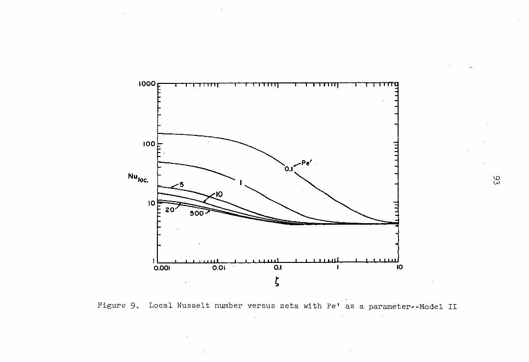
1000 r I I I I I

I I I I I I I

0.001 0.01

5

io u;

Figure 9. Local Nusselt number versus zeta with Pe' as a parameter--Model II

94

n—m—r~r

CURVE

8

10 12 14 16 18 20 22 24

Z/C

Figure 10. Variation of local Nusselt number with axial distance and Pe'--Model II

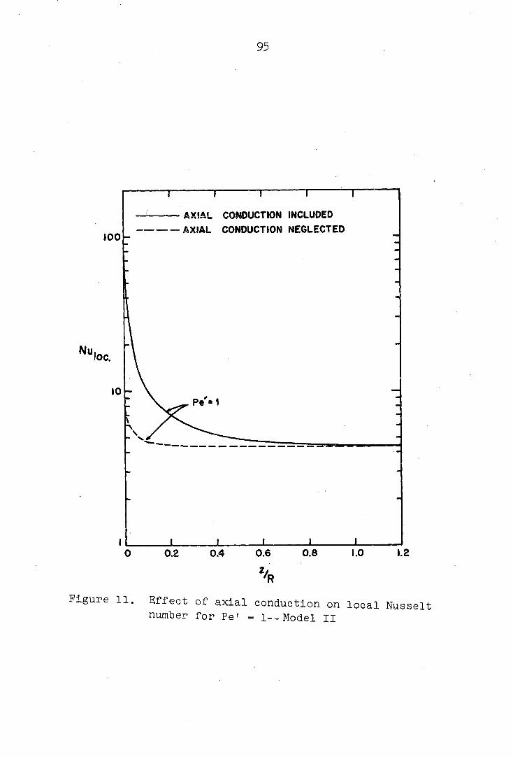
95

— AXIAL CONDUCTION INCLUDED

— AXIAL CONDUCTION NEGLECTED 100

loc.

10 P e » 1

1.2 1.0 0.6 0.8 0 0.2 0.4

Figure 11. Effect of axial conduction on local Nusselt number for Pe' = 1--Model II

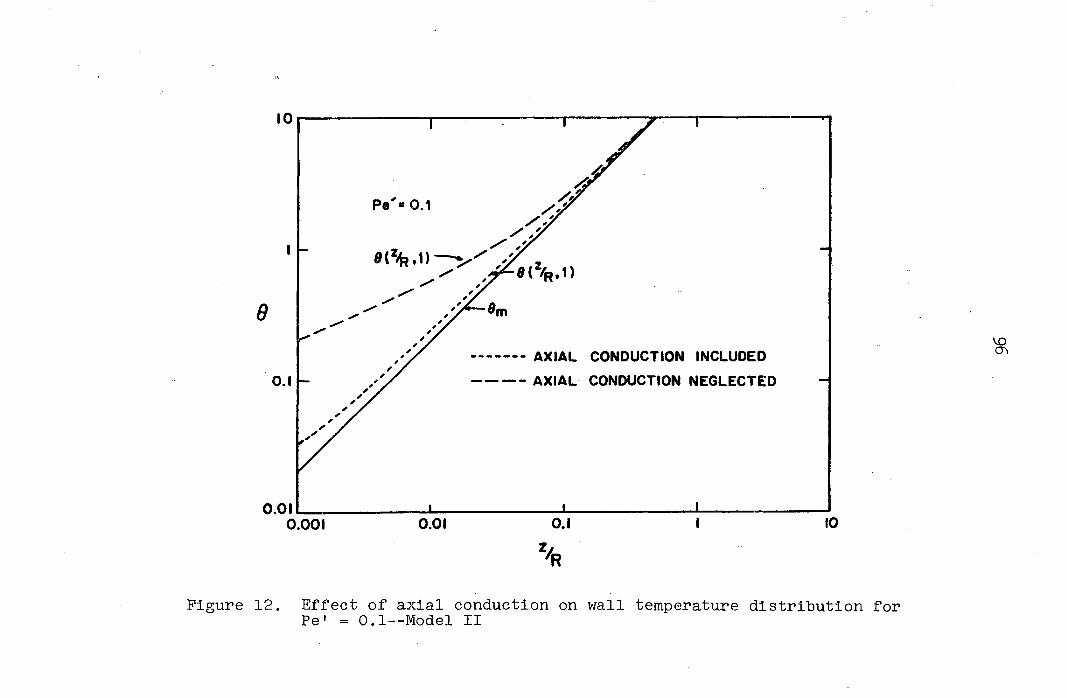
AXIAL CONDUCTION INCLUDED

AXIAL CONDUCTION NEGLECTED

Figure 12. Effect of axial conduction on wall temperature distribution for Pe1 = 0.1—Model II

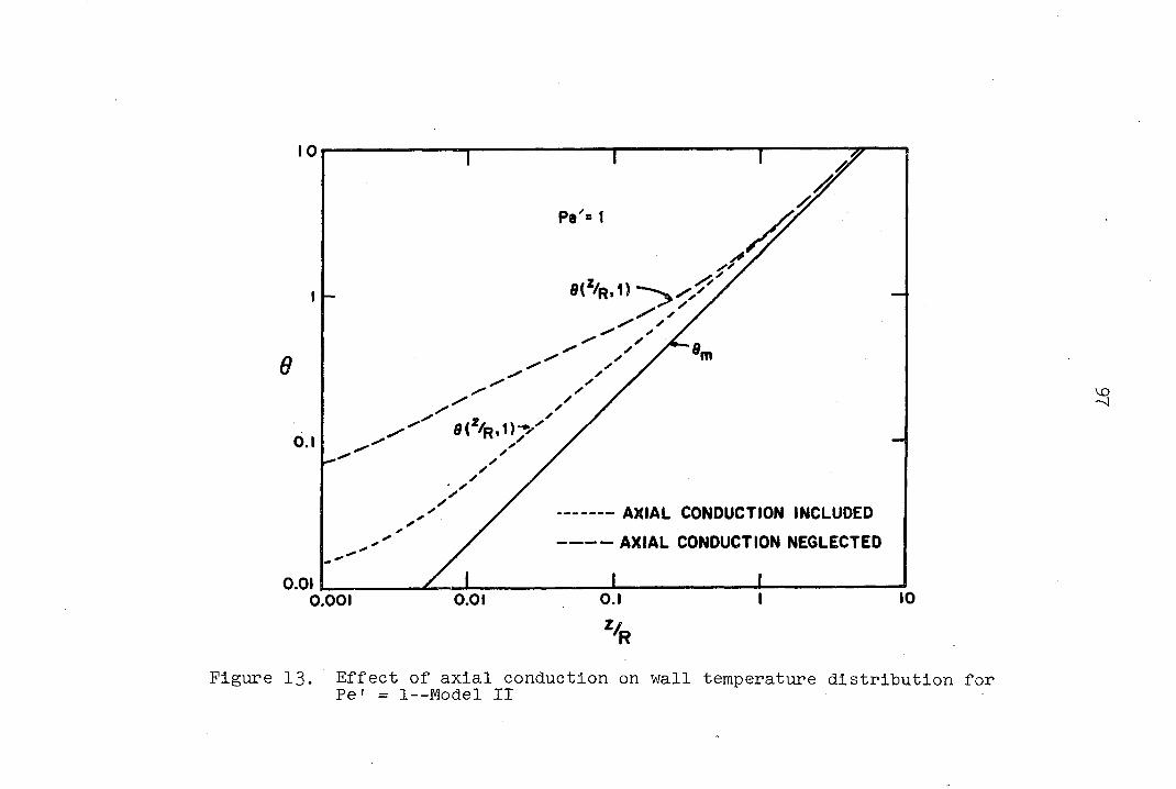
0.1

AXIAL CONDUCTION INCLUDED

AXIAL CONDUCTION NEGLECTED

0.01 0.1 0.01 0.001

Z/r

Figure 13. Effect of axial conduction on wall temperature distribution for Pe1 = l--Model II

10

AXIAL CONDUCTION INCLUDED

— AXIAL CONDUCTION NEGLECTED

I -

e

0.1 -

Pe'= 10

81%,1)

0.01

erW)

0.001 10

yo co

Figure 14. Effect of axial conduction on wall temperature distribution for Pe1 = 10--Model II

the effect has diminished considerably. When the value of

Pe1 is 50 or greater the axial conduction effect associated

with the wall temperature becomes negligible.

The approximate solution to Model II described Model I

at small values of zeta and approached Model II when zeta

became large.

The error associated with matching the condition that

6(C, 5) = 0 at C = 0 for § = 0 to § = 1 was somewhat higher

for the fully-developed laminar flow model than for the

plug flow model. This may be attributed directly to the

complication given by the parabolic velocity distribution

and the difficulty in approximating the eigenfunctions by

a series of Bessel functions. The maximum error at the

inlet to the heated section of the tube was found at the

tube wall. At Pe' = 0.1, 1, 10 and 100 the corresponding

values of 0(0,1) were 0.1028 x 10 \ 0.1038 x 10 \

0.11403 x 10~\ and 0.4661 x 10~\ respectively. The

values of 6m(0,§) increase from -0.2917 at § = 0- to 0.4583

at § = 1. The errors found at the intermediate points

were considerably less than at the wall. The error at

high Pe1 values would be expected to be larger because the

solution contained only eight terms in the summation for

0d and the last four were approximated by using the eigen­

functions and expansion coefficients for Pe1 =10. The

results are in agreement with those for Model I. The

100

errors in the solution also show up in the calculation of

the mixed-mean dimensionless temperature. At small values

of zeta, 6m becomes negative, consequently the corresponding

values of local Nusselt number are not as large as would be

expected.

A solution to Model II using X^ ^ 0 was tested at

Pe1 =10 and the results were invalid„ At small values of

zeta, the Nusselt number became negative and the thermal

profiles did not satisfy the inlet condition. Therefore,

the solution derived using X^ = 0 was concluded to be cor­

rect .

Thermal entrance region - Model I and Model II

The dependence of the thermal entrance length on Pe1

can be determined for both models from the plots of the

local Nusselt number versus zeta. In addition to the

thermal entry length for a 1.05 ratio of the local Nusselt

number to the fully-developed Nusselt number, the length

required for the ratio to reach 1.02 was evaluated. The

results for both Nusselt ratios are given in Figure 15.

The thermal entry length for Model I is slightly larger

than that for Model II. The data are in agreement with

Petukhov and Tsvetkov (56) who used a 1.01 Nusselt ratio

and predicted thermal entry lengths of 0.91, 1.12, 2.1,

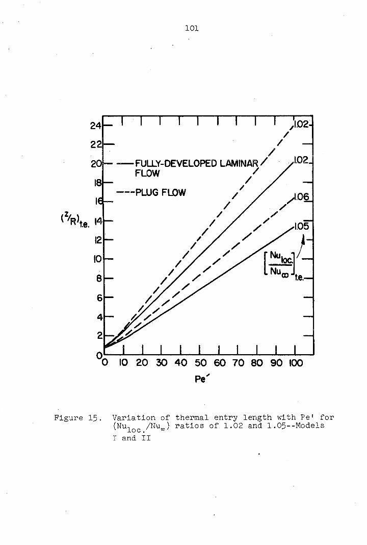
101

m—n—i—i—i—r™1"

(%. ,4

FULLY-DEVELOPED LAMINAR/ FLOW

PLUG FLOW

® te.—

I I I I I I I I I I

0 10 20 30 40 50 60 70 80 90 100

Pe'

Figure 15. Variation of thermal entry length with Pe1 for (Nu, /Nu ) ratios of 1.02 and 1.05--Models loc. °> I and II

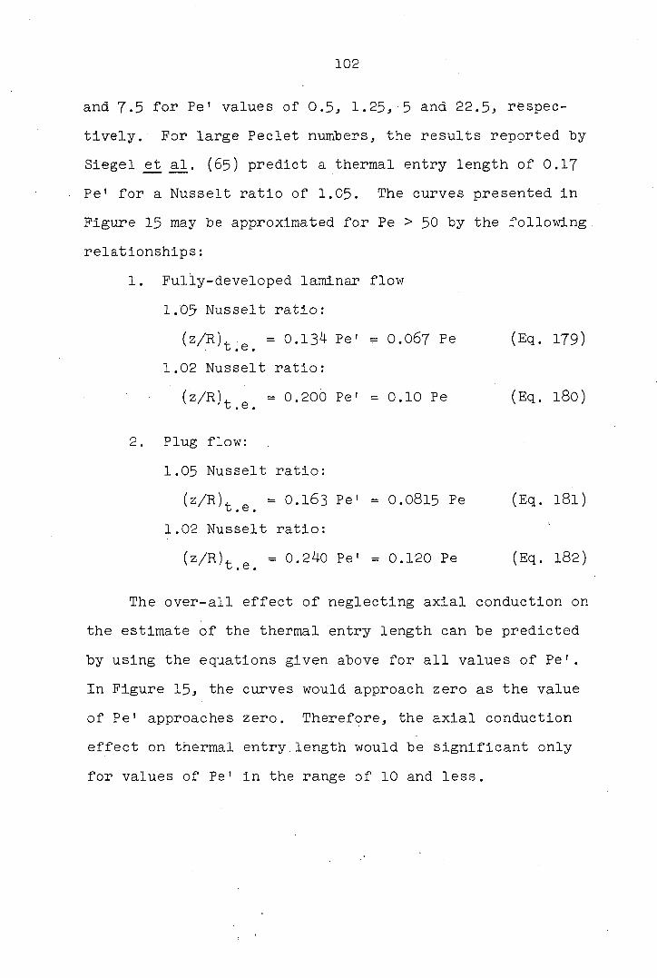
102

and 7.5 for Pe1 values of 0.5, 1.25, 5 and 22.5, respec­

tively. For large Peclet numbers, the results reported by

Siegel et_ al. (65) predict a thermal entry length of 0.17

Pe1 for a Nusselt ratio of 1.05. The curves presented in

Figure 15 may be approximated for Pe > 50 by the following.

relationships :

1. Fully-developed laminar flow

1.05 Nusselt ratio :

(z/R)t e = 0.134 Pe' = 0.067 Pe (Eq. 179)

1.02 Nusselt ratio :

(z/R)^ g = 0.200 Pe' = 0.10 Pe (Eq. 180)

2. Plug flow:

1.05 Nusselt ratio :

(z/R)t e = 0.163 Pe' = 0.0815 Pe (Eq. l8l)

1.02 Nusselt ratio :

(z/R)t e = 0.240 Pe' = 0.120 Pe (Eq. 182)

The over-all effect of neglecting axial conduction on

the estimate of the thermal entry length can be predicted

by using the equations given above for all values of Pe'.

In Figure 15, the curves would approach zero as the value

of Pe' approaches zero. Therefore, the axial conduction

effect on thermal entry length would be significant only

for values of Pe' in the range of 10 and less.

103

Constant Wall Temperature Models

The computer programs used to calculate the heat

transfer parameters for Model III (plug flow) and Model IV

(fully-developed laminar flow) are listed in Figures 36

and 39 in the Appendix. The pertinent computer output data

are available elsewhere (30).

Model III. Plug flow

The local Nusselt number for Model III with Pe' as a

parameter is given in Figure 16 with zeta as the inde­

pendent variable. For all values of Pe1 the Nusselt number

asymptotically approaches 5-783 as zeta becomes large. The

difficulty in calculating Nusselt numbers for small values

of zeta is shown by the curves leveling off when zeta be­

comes small. The effect of neglecting axial conduction on

the Nusselt number is shown in Figure 17 for Pe1 =1 and

Pe ' = 10. When Pe' j> 50, this effect is negligible. At

this point it might be assumed that neglecting axial con­

duction would tend to underestimate the heat transfer be­

cause the heat transfer coefficient is larger when axial

conduction is included. This conclusion was reached by

Schneider (63) in an analysis of this model. The reasoning

was based on the fact that mean Nusselt numbers for a

I 0,001 0.01 ai 1.0 100

Figure 16. Local Nusselt number versus zeta with Pe1 as a parameter--Model III

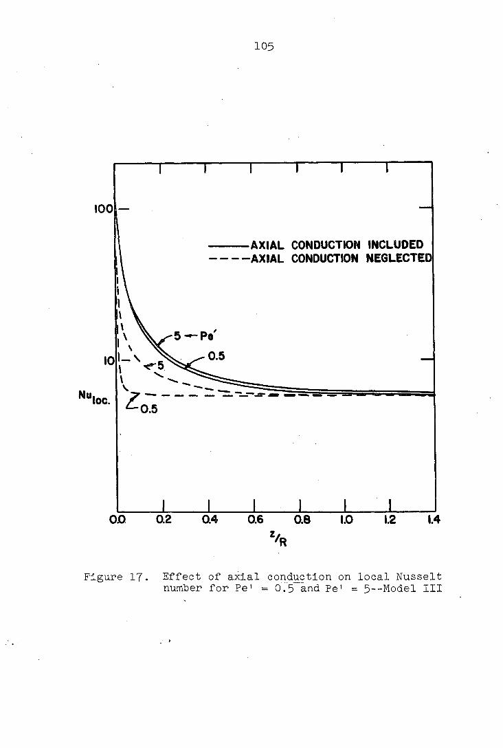
105

100

AXIAL CONDUCTION INCLUDED - -AXIAL CONDUCTION NEGLECTED

0.5 t - \

0.5

0.2 0.0 0.4 0.6 0.8 1.0 1.2 1.4

Figure 17. Effect of axial conduction on local Nusselt number for Pe1 =0.5 and Pe' = 5--Model III

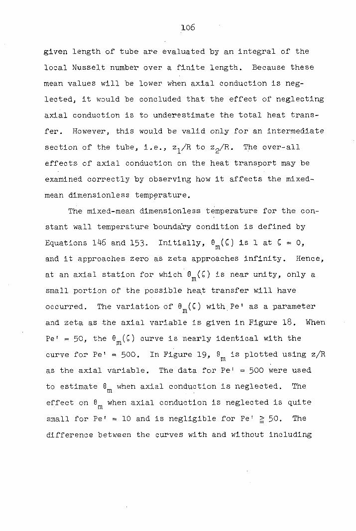
106

given length of tube are evaluated by an integral of the

local Nusselt number over a finite length. Because these

mean values will be lower when axial conduction is neg­

lected, it would be concluded that the effect of neglecting

axial conduction is to underestimate the total heat trans­

fer . However, this would be valid only for an intermediate

section of the tube, i.e., z^/R to Zg/R. The over-all

effects of axial conduction on the heat transport may be

examined correctly by observing how it affects the mixed-

mean dimensionless temperature.

The mixed-mean dimensionless temperature for the con­

stant wall temperature boundary condition is defined by

Equations 146 and 153. Initially, 8^(G) is 1 at C = 0,

and it approaches zero as zeta approaches infinity. Hence,

at an axial station for which ®m(0 is near unity, only a

small portion of the possible heat transfer will have

occurred. The variation of 8^(G) with Pe1 as a parameter

and zeta as the axial variable is given in Figure 18. When

Pe1 = 50, the 8^(G) curve is nearly identical with the

curve for Pe' = 500. In Figure 19, 6m is plotted using z/R

as the axial variable. The data for Pe1 = 500 were used

to estimate 6^ when axial conduction is neglected. The

effect on 6^ when axial conduction is neglected is quite

small for Pe1 =10 and is negligible for Pe' >50. The

difference between the curves with and without including

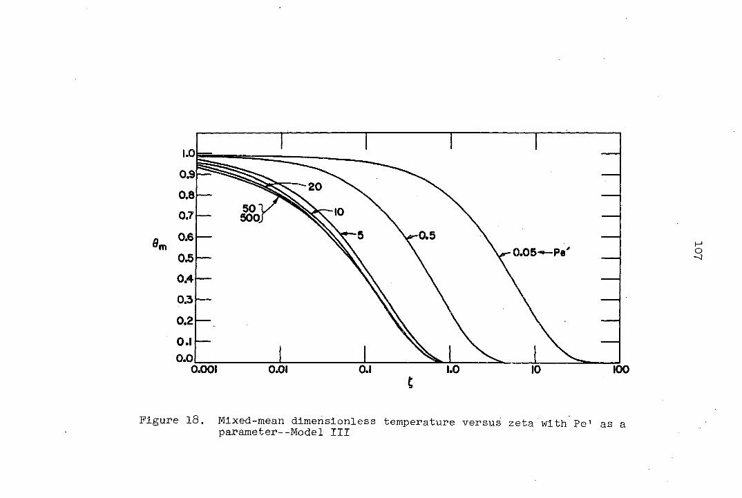
0.9 20

0.8 50" 500 0.7

0.5 m 0.05 0J5

0.4

0.3

0.2

0.1 0.0

,001 0.01 1.0 100 C

Figure 18. Mixed-mean dimensionless temperature versus zeta with Pe1 as a parameter--Model III

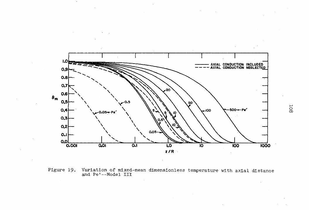
AXIAL CONDUCTION INCLUDED AXIAL CONDUCTION NEGLECTED

8 m

0.05-1-Pe

0.001

500*-Pe'

1000

Figure 19. Variation of mixed-mean dimensionless temperature with axial distance and Pe'--Model III

109

axial conduction show conclusively that the mixed-mean

dimensionless temperature is underestimated and that the

heat transfer is overestimated when axial conduction is

neglected.

The calculation of the total heat transport may be

done easily by using the Q-ratio as defined by Equation

157. The Q-ratio with Pe1 as a parameter is given in

Figures 20 and 21 using axial variables of zeta and z/R,

respectively. The asymptotic value for the Q-ratio for

all Pe' as the axial distance becomes large is n/4. These

figures provide a convenient set of curves for interpola­

tion at intermediate Pe' values. The actual dependent

variable is Q/[k(Tw - T )] and this is plotted with Pe' as

a parameter in Figure 22. When the fluid properties, Pe',

and the inlet and wall temperature conditions are speci­

fied, the total heat transport, Q, may be calculated easily

without resorting to the use of Nusselt numbers.

The error in matching the inlet condition of 0(G,5) = 1

for 0 < § < 1 at C =0 was checked. At the wall, 9(0,1) =

-O.I692 x 10"^ and at the tube center, 6(0,0) = 0.8755.

The latter condition represented the maximum error on the

interval with radial increments of 0.05, and usually the

deviation from unity was only 2 or 3 per cent. The inte­

gral of the deviation from unity over the interval was

negligible.

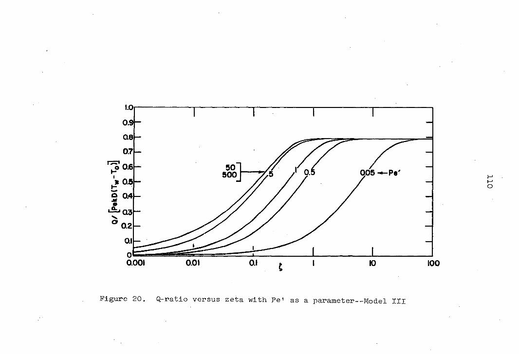
1.0

0.9-

Q8

0.7

50 500 005

s 0.5

e o.4 Q.

Q3

0.2

0.001 0.01 0.1 10 100

Figure 20. Q-ratio versus zeta with Pe1 as a parameter—Model III

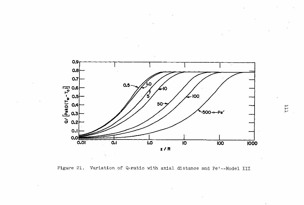
1000 z / R

Figure 21. Variation of Q-ratio with axial distance and Pe1--Model III

1000

100

50 100

0.01 0.1 100 1000

Figure 22. Q/[k(Tw - T )] versus z/R with Pe' as a parameter--Model III

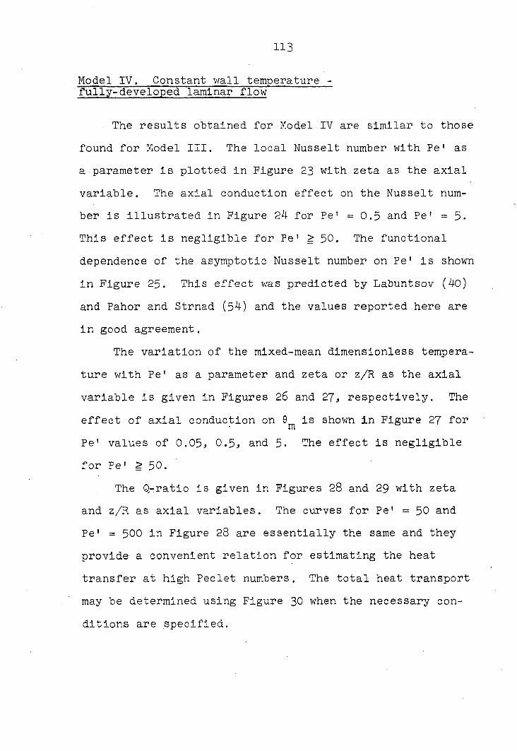
113

Model IV. Constant wall temperature -fully-developed laminar flow

The results obtained for Model IV are similar to those

found for Model III. The local Nusselt number with Pe1 as

a parameter is plotted in Figure 23 with zeta as the axial

variable. The axial conduction effect on the Nusselt num­

ber is illustrated in Figure 24 for Pe' =0.5 and Pe' = 5.

This effect is negligible for Pe' 2 50. The functional

dependence of the asymptotic Nusselt number on Pe1 is shown

in Figure 25. This effect was predicted by Labuntsov (40)

and Pahor and Strnad (54) and the values reported here are

in good agreement.

The variation of the mixed-mean dimensionless tempera­

ture with Pe1 as a parameter and zeta or z/R as the axial

variable is given in Figures 26 and 27, respectively. The

effect of axial conduction on 0m is shown in Figure 27 for

Pe1 values of 0.05, 0.5, and 5. The effect is negligible

for Pe1 2? 50.

The Q-ratio is given in Figures 28 and 29 with zeta

and z/R as axial variables. The curves for Pe' =50 and

Pe1 = 500 in Figure 28 are essentially the same and they

provide a convenient relation for estimating the heat

transfer at high Peclet numbers. The total heat transport

may be determined using Figure 30 when the necessary con­

ditions are specified.

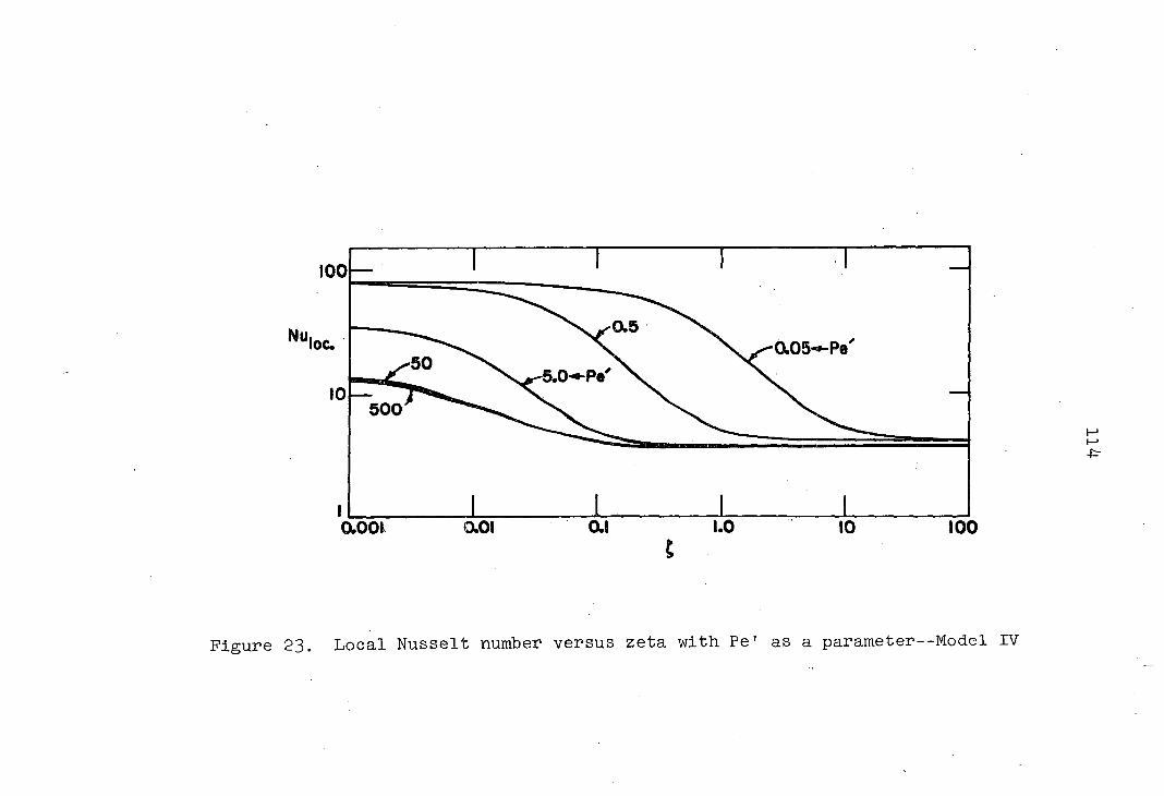
100

0.5

50

500

1.0 100 0.01

t

Figure 23. Local Nusselt number versus zeta with Pe' as a parameter—Model IV

115

100

AXIAL CONDUCTION INCLUDED AXIAL CONDUCTION NEGLECTED

Pe *5

e "0.5

0.2 0.4 0.6 0.8 1.0 1.2

z / R

Figure 24. Effect of axial conduction on local Nusselt number for Pe' = 0.5 and Pe' = 5—Model IV

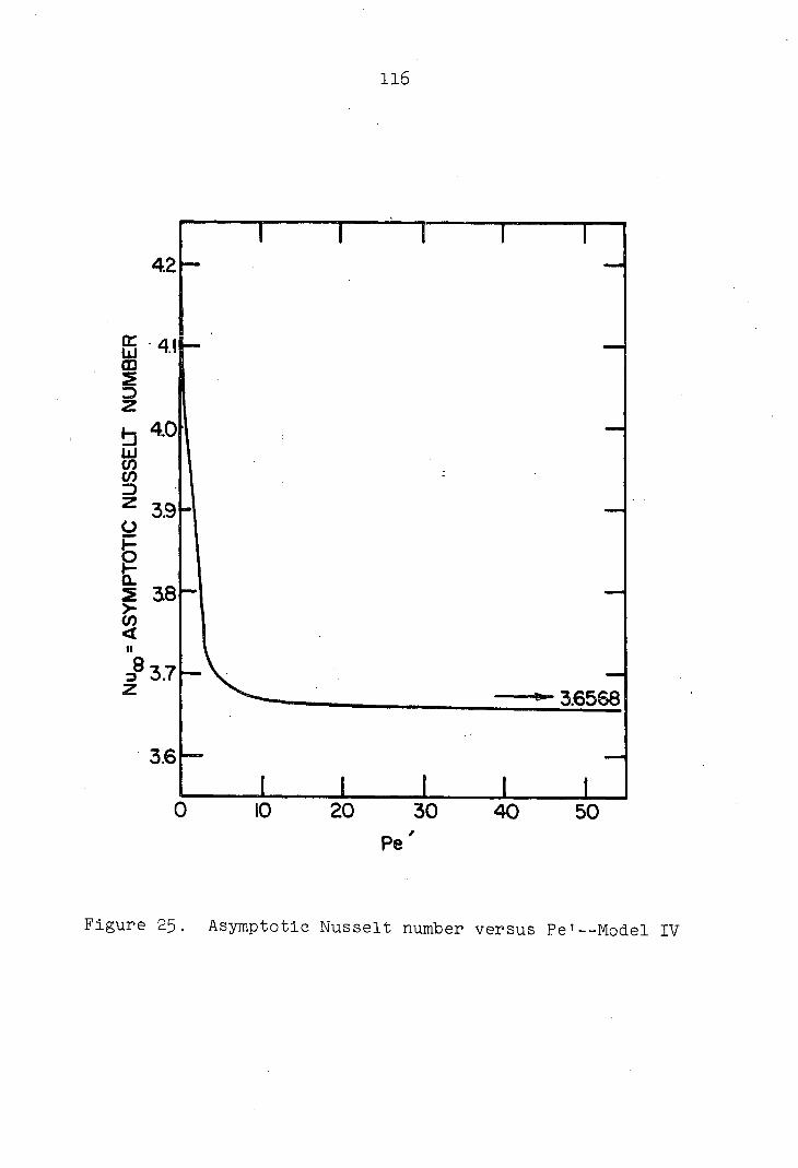
116

4.2

4.1

4.0

3.9

*•" 3.6568

3.6

0 10 20 30 40 50

Figure 25. Asymptotic Nusselt number versus Pe'--Model

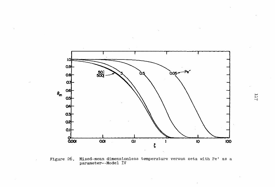
50 0.05 OB

0.7

OJ6

05-

04-

03

02

0001 Ql 100

Figure 26. Mixed-mean dimensionless temperature versus zeta with Pe1 as a parameter—Model IV

I • I ( 111 I I I I I 1111 I— - AXIAL CONDUCTION INCLUDED

- AXIAL CONDUCTION NEGLECTED

1.0

0.8 -X

0.6 0.05 E

Q3 500

0.4 -

0.5

0.2

• y O.l 10 0.001 0.01 100 1000

Figure 27. Variation of mixed-mean dimensionless temperature with axial distance and Pe1--Model IV

1.01 1—i—i I I 1111 1—i—i i i n H 1—i—TT

0.8 -

|2 & 0.6

£L 0.4

0.2 -

0.001 0.01

£

Figure 28. Q-ratio versus zeta with Pe1

i—i .linn » i i » 1111

0.05— H H VO

100

parameter--Model IV

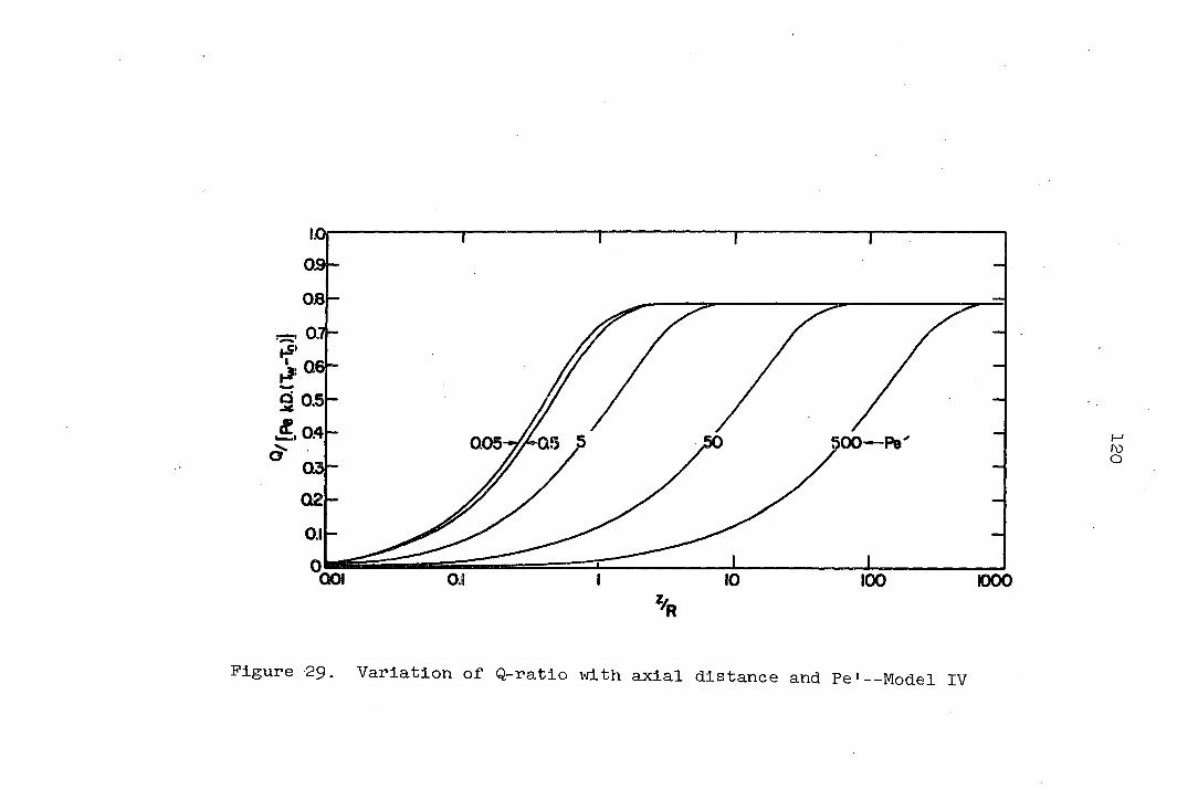
09-

03

<5 0.5

005 03-

02

QOI 100 1000

Figure; 29. Variation of Q-ratio with axial distance and Pe' Model IV

121

1000 00

50 iOO

i f 10

0.5

0.05

QOI 0.01 Ql 10 100 1000

Figure 30. Q/ C k (Tw - T )] versus z/R with Pe' as a

parameter--Model IV

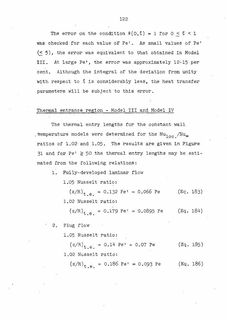
122

The error on the condition 0(0,§) = 1 for 0 < § < 1

was checked for each value of Pe1. As small values of Pe'

(< 5 ) * the error was equivalent to that obtained in Model

III. At large Pe', the error was approximately 12-15 per

cent. Although the integral of the deviation from unity

with respect to § is considerably less, the heat transfer

parameters will be subject to this error.

Thermal entrance region - Model III and Model IV

The thermal entry lengths for the constant wall

temperature models were determined for the Nu1qc /Nuœ

ratios of 1.02 and 1.05. The results are given in Figure

31 and for Pe1 ^ 50 the thermal entry lengths may be esti­

mated from the following relations :

1. Fully-developed laminar flow

1.05 Nusselt ratio:

(z/R)t e = 0.132 Pe' = 0.066 Pe

1.02 Nusselt ratio :

(Eq. 183)

(z/R)t e = 0.179 Pe' = 0.0895 Pe (Eq. 184)

2. Plug flow

1.05 Nusselt ratio :

(z/R)t e = 0.14 Pe' = 0.07 Pe

1.02 Nusselt ratio:

(Eq. 185)

(z/R)t e = 0.186 Pe' = 0.093 Pe (Eq. 186)

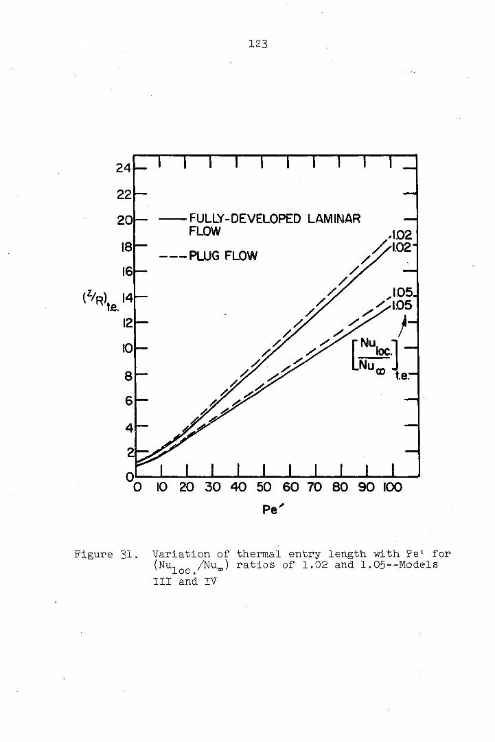
123

24 —

22

FULLY-DEVELOPED LAMINAR FLOW

20

— PLUG FLOW

loc.

figure 31. variation of thermal entry length with Pe' for (Nuioc /Nuœ) ratios of 1.02 and 1.05--Models

III and IV

124

The effect of neglecting axial fluid conduction on the

thermal entry length may be predicted by applying the

above equations for small values of Pe'. The effect be­

comes significant for Pe1 g 10.

The heat transfer which occurs in the thermal entry

region may be determined for a given Pe1 using Figures 29

and 31. The ratio of the Q-ratio at (z/R)^ g over rr/4 is

a measure of the fraction of available heat transfer which

occurs in the thermal entrance region. The per cent of the

total heat transport at (z/R)^ g versus Pe1 is given in

Figure 32. For Model III at large Pe1 values, approxi­

mately 50 to 60 per cent of the possible heat transfer

occurs in the thermal entrance region. For Model IV at

large Pe1 values, approximately TO per cent of the possible

heat transfer occurs in the thermal entrance region. These

approximate figures illustrate the utility in using the

Q-ratio and the corresponding ambiguity in using Nusselt

numbers for predicting heat transfer with the constant

wall temperature models. This conclusion is emphasized

further by the fact that for Model IV, the asymptotic

Nusselt number depends on the Peclet number.

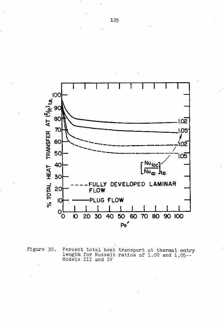
125

I I I I I I I I I

100 ™ «

s

I 3

I

FULLY DEVELOPED LAMINAR FLOW -PLUG FLOW

I I I I I I I I I I

10 20 30 40 50 60 70 80 90 100 Pe'

Figure 32. Percent total heat transport at thermal entry length for Nusselt ratios of 1.02 and 1.OS-Models III and IV

126

DISCUSSION

The results presented for the various models should

be interpreted from a qualitative viewpoint rather than a

quantitative viewpoint. The analyses of the models are

based on numerous assumptions ; however, the general trend

of the effect of axial conduction on heat transfer is indi­

cated. The results should provide preliminary information

applicable to the experimental measurement or calculation

of heat transfer at low Peclet numbers.

One of the assumptions which is not likely valid for

small values of Pe' is that the fluid temperature is uni­

form at the inlet to the heated section of the tube. It is

recognized that for Pe' = 0 the problems degenerate to pure

conduction heat transfer. A condition of continuity of the

axial heat flux at z = 0 could have been used with the con­

dition that T = Tq (for all r) at z = -00. This would re­

quire two separate solutions and thus both the positive

and negative eigenvalues from the infinite system of equa­

tions could be used. This approach would be applicable

particularly to the fully-developed laminar flow models.

However, for plug flow at the entrance to a heat exchanger,

the plug flow models probably would be valid at least

until the velocity profile becomes developed.

The difficulty associated with the eigenvalue

127

calculations at large Pe1 might be remedied by using a

Gauss-Seidel iteration with relaxation as discussed by

Hildebrand (27). This routine would require programming

the computer to use judgment in the relaxation process and

the computation time would increase accordingly.

If the eigenfunction expansion method is employed in

other problems, some difficulty could arise in obtaining

the integral transforms in compact form. If a solution ex­

pansion is assumed and evaluated in the partial differen­

tial equation and then integral transforms taken, the

transpose of the infinite system of equations can arise.

This phenomenon was noted in the checking of the solution

given by Singh (67) using Equations 158 and 96 to obtain

Equation 159• Therefore, it is expedient to derive the

infinite system of equations directly from the development

given in the theoretical section.

128

CONCLUSIONS

The following conclusions may be reached as a result

of this investigation:

1. For a constant wall heat flux boundary condition,

the effect of neglecting axial conduction on heat transfer

in the thermal entrance region is to overestimate the wall

temperature distribution. The effect is negligible when

the Peclet number is greater than 100.

2. For a constant wall temperature boundary condi­

tion, the effect produced by neglecting axial conduction

is to overestimate the heat transfer and to underestimate,

the mixed-mean dimensionless temperature.

3. The asymptotic Nusselt numbers for either constant

wall heat flux or constant wall temperature boundary con­

dition are the same when axial conduction is included or

neglected.

4. The asymptotic Nusselt number for fully-developed

laminar flow in a tube with constant wall temperature was

found to depend on the Peclet number. When the Peclet

number is greater than ten, the asymptotic Nusselt number

essentially becomes a constant value of 3.6568.

5. The thermal entrance length is a function of the

Peclet number and linearly increases for values of the

Peclet number greater than 100. For small values of the

129

Peclet number, the thermal entry length is underestimated

when axial conduction is neglected.

6. For plug flow in a tube with constant wall temper­

ature, approximately 70 per cent of the total heat transfer

possible will occur in the thermal entrance region. For

fully-developed laminar flow, approximately 50 to 60 per

cent of the total heat transfer will occur in the thermal

entrance region. Consequently, it is better to calculate

the heat transfer directly without using Nusselt numbers

and this may be done provided that the Peclet number,

fluid properties, and the inlet and wall temperatures are

specified.

7. The method of solution based on generalized

Sturm-Liouville theory was found to work satisfactorily

for small values of the Peclet number. However, as the

Peclet number was increased, the eigenvalue computations

became difficult and instability in the iterative method

of calculation occurred. A reasonable explanation for

this difficulty is that the matrix becomes ill-conditioned

when the Peclet number becomes large and also that there

is a corresponding loss of significant figures in the cal­

culations.

130

RECOMMENDATIONS

After careful analysis of the results of this investi­

gation, the following recommendations for further work are

made:

1. A relaxation method should be applied to the sys­

tem of algebraic equations to calculate the higher eigen­

values and corresponding sets of associated coefficients

for large Peclet numbers.

2. The problem for constant wall temperature or con­

stant wall heat flux with fully-developed laminar flow

should be studied for an inlet condition of continuity of

the axial heat flux and a boundary condition of T = Tq at

z = —œ. This model would be applicable to very small

values of the Peclet number.

3. The solution to the partial differential equation

including axial conduction could be examined by using

finite differences and the results compared with those re­

ported here. Such.an analysis would provide preliminary

information for a larger study in which the variation of

fluid properties is included.

4. The method of solution used for the fully-

developed laminar flow models could be applied to asso­

ciated heat or mass transfer problems.

131

5. In all the models it was assumed that the re­

sistance of the wall to heat transfer was negligible. The

method of solution could be extended to heat transfer

problems for which the wall resistance is finite, an ex­

ample of which is a ceramic heat exchanger.

6. For the constant wall temperature models, the

calculated values of Q-ratio will yield the total heat

transport, Q, for the interval (0, z/R). The wall heat

transport, should be evaluated using the relation

0* = Q - (Qlz=o " Qlz=z)

where

Qlz=z* =-nj"o k - rdr

and z * is a prescribed value of z. Hence, the total heat

transported through the tube wall can be determined.

132

NOMENCLATURE

lower limit of an interval

an expansion coefficient

a prescribed constant

a prescribed constant

2 cross-section area of conduit, ft

element of the i^ row of a matrix

upper limit of an interval

a prescribed constant

a prescribed constant

i^ coefficient

m^ associated coefficient of the n^

eigenfunction

specific heat at constant pressure per unit

mass, Btu/lb -°F ' m

specific heat at constant volume per unit mass,

Btu/lb -°F ' m

tube diameter, ft

inside tube diameter, ft

outside tube diameter, ft

a function, see Equation 162

a function, see Equation 33

a function, see Equations 31, 34, 35, 36, and 37 p

gravitational acceleration vector, ft/sec

133

G uniform heat generation per unit volume,

Btu/sec-ft^

G* dlmenslonless uniform heat generation term, see

Equation lj6

h film heat transfer coefficient, Btu/hr-ft-°F

h- oc local film heat transfer coefficient, Btu/sec-°F

H a function, see Equation 38

H total average enthalpy change, Btu/sec

J Bessel function of the first kind of order v.

k thermal conductivity, Btu-ft/sec-°F-ft2

k^ fluid thermal conductivity, Btu-ft/sec-°F-ft2

k wall thermal conductivity, Btu-ft/sec-°F-ft2

K ratio, at a cross section, of total axial molecu­

lar and eddy conductivity of fluid and

apparatus to total axial molecular conduc­

tivity of fluid

L length of tube, ft; characteristic length, ft

Lg thermal starting length, ft, see Equation 29

hydrodynamic starting length, ft, see Equation 30

Nu Nusselt number, hD/k

Nu , local Nusselt number, h, D/k loc. ' loc. ' .

Nu , Nusselt number derived bv use of T_ v , m. b. * m. u.

qD/kf(Tw - ), see Equation 18

NUprobe Nusselt number derived by u'se of Tproke-

qD/k^(T^ - Tprotg), see Equation 1?

134

p P pressure, lbf/ft

Pe Peclet number, 2RC V^/k p z'

Pe' Peclet number/2, RC^V^/k

Pr Prandtl number, |a6 /k

q heat flux, Btu/sec-ft2

q' heat flux per unit length of tube, Btu/hr-ft

qr heat flux in radial direction, Btu/sec-ft

qz heat P

flux in axial direction, Btu/sec-ft

q0 heat 2 flux in angular direction, Btu/sec-ft

Q heat transport, Btu/sec

Q average heat transfer, Btu/sec

r tube radial position variable, ft

R tube radius, ft

Re Reynolds number, 2RV p/n

S 2 cross-section area of tube, ft

t fluctuating temperature variable, °F

T point temperature of fluid, °F

Tb bulk temperature of fluid, °F, see Equation

Tb average calorimetric temperature of fluid, °'.

see Equation 3

Tiniet inlet temperature of fluid, °P

H mixing-box mean temperature of fluid, °P, see

Equation 14

Tpro^e probe mean temperature of fluid, °F, see

Equation 12

135

T energy mean temperature of fluid, °F, see energy

Equation 9

Tm mean fluid temperature, °F

T wall temperature, °F w

Tq inlet temperature of fluid, °F

T time average point temperature of fluid, °F

Un eigenfunction corresponding to n^*1 eigenvalue

V fluid velocity vector, ft/sec

V point fluid velocity in the z-direction, ft/sec

Vz average fluid velocity in the z-direction, ft/sec

wn an arbitrary constant, see Equation 42

W electrical heat input, Btu/sec

Wq dlmenslonless viscous dissipation term, see

' ' Equation 177

x independent variable

X a function of x

V Bessel function of the second kind of order v

z axial position variable, ft

z1 axial variable, z/R

a an eigenvalue

6^ a temperature correction factor, °F, see

Equation 2

A a change operator, a determinant

c a constant

Q dlmenslonless axial position variable, (z/R)/Pe'

136

0 dimensionless temperature, (T - T )/qR/k; dimen-l

sionless temperature, (T - T )/(T - T ); W O W

angular variable, degrees

6m mixed-mean dimensionless temperature

X an eigenvalue

la fluid viscosity, lb /ft-sec

§ dimensionless radial position variable, r/R

an eigenfunction

rr a constant, 3.14159265

p fluid density, lb /ft^

T time, sec

t shear stress tensor, lb^/sec -ft

2 t r-momentum flux in z-direction, lb /sec -ft rz irr

137

LITERATURE CITED

1. Abramowitz, M. On the solution of the differential equation occurring in the problem of heat convection in laminar flow through a tube. J. Math. Phys. 32: 184-189. 1953.

2. Abramowitz, M., Cahill, W. P., and Wade, C. Heat transfer in laminar flow through a tube. U.S. Nat. Bur. Stds. J. Res. 62: 101-105. 1959.

3. Akins, R. G. and Dranoff, J. S. Experimental study of laminar flow heat transfer with prescribed wall heat flux. Am. Inst. Chem. Eng. J. 9- 624-629. 1963.

4. Bird, R. B. Theory of diffusion. Advances in Chemical Engineering 1: 156-239. 1956.

5. Bird, R. Byron, Stewart, Warren E., and Lightfoot, Edwin N. Transport phenomena. New York, New York, John Wiley and Sons, Inc. i960.

6. Boessenroth, Iva. IBM-7074 computer program: MATINV(REVISED), Distribution No. 707402631300011. Ames, Iowa, Computer Services Group, Institute for Atomic Research, Iowa State University of Science and Technology. February 15, 1963.

7. Boessenroth, Iva. IBM-7074 computer program: special purpose series of Bessel functions for orders zero and one, Distribution No. 707401631300003. Ames, Iowa, Computer Services Group, Institute for Atomic Research, Iowa State University of Science and Technology. January 22, 1963.

8. Bowman, Frank. Introduction to Bessel functions. New York, New York, Longmans, Green and Company. 1938.

9. Brinkman, H. C. Heat effects in capillary flow. I. Appl. Sci. Res. Sec. A, 2: 120-124. 1950.

138

10. Brooks, R. D. and Friedlander, S. K. Heat transfer correlations for liquid metals. In Hogerton, J. F. and Brass, R. C., eds. The reactor handbook. Vol. 2. pp. 277-286. U.S. Atomic Energy Commission Report AECD-3646. [Technical Information Service Extension, AEC]. 1955.

11. Brown, G. M. Heat or mass transfer in a fluid in laminar flow in a circular or flat conduit. Am. Inst. Chem. Eng. J. 6: 179-183. i960.

12. Chelemer, Harold. Effect of gas entrainment on the heat transfer characteristics of mercury under turbu­lent flow conditions. Unpublished Ph.D. thesis. Knoxville, Tennessee, Library, University of Tennessee. 1955.

13. Churchill, Ruel V. Fourier series and boundary value problems. 2nd ed. New York, New York, McGraw-Hill Book Company, Inc. 1963.

14. Dennis, S. C. R. The determination of eigenfunctions of the Sturm-Liouville equation. Quarterly Journal of Mechanics and Applied Mathematics 9: 371-383-1956.

15. Dennis, S. C. R. and Foots, G. A solution of the heat transfer equation for laminar flow between parallel plates. Quarterly of Applied Mathematics 14: 231-236. 1956.

16. Does de Bye, J. A. W. Van der and Schenk, J. Heat transfer in laminary flow between parallel plates. Appl. Sci.. Res. Sec. A, 3: 308-316. 1953.

17. Dranoff, J. S. An eigenvalue problem arising in mass and heat transfer studies. Math. Computation 15: 403-409. 1961.

18. Dwyer, 0. E. Heat exchange in LMF power reactor sys­tems. Nucleonics "J: 30-39. 1954.

19. Eagle,.A. and Ferguson, R. M. On the coefficient of heat transfer from the internal surface of tube walls. Roy. Soc. (London) Proc. Sec. A, 127: 540-566. 1930.

20. Eckert, E. R. G. and Drake, R. M. Heat and mass transfer. 2nd ed. New York, New York, McGraw-Hill Book Company, Inc. 1959.

139

21. Goldstein, S. Modern developments in fluid dynamics. Vol. 2. London, Oxford University Press. 1938..

22. Graetz, L. Uber die warmeleitfâhigkeit von fliïssigkeiten. Annalen der Physik Chemie 25: 337- ' 357. 1885.

23. Gray, Andrew and Mathews, G. B. A treatise on Bessel functions and their applications to physics. 2nd ed. New York, New York, Macmillan and Company. 1922.

24. Gray, I. L. Design and fabrication of a 2100°F forced convection lithium test loop. U.S. Atomic Energy Commission Report BNL-756: 326-352. Brookhaven National Laboratory, Upton, New York. 1962.

25. Grober, H., Erk, S., and Grigull, U. Fundamentals of heat transfer. New York, New York, McGraw-Hill Book Company, Inc. 1961.

26. Harvard University Computational Laboratory. Tables of Bessel functions of the first kind of orders zero and one. Cambridge, Massachusetts, Harvard University Press. 1947.

27. Hildebrand, F. B. Introduction to numerical analysis. New York, New York, McGraw-Hill Book Company, Inc. 1951.

28. Hohn, F. E. Elementary matrix algebra. New York, New York, Macmillan Company. 1961.

29. Holman, Kermit. Research Notebook No. 62-172 KH-1. (Manuscript) Ames, Iowa, Document Library, Institute for Atomic Research, Iowa State University of Science and Technology. 1962.

30. Holman, Kermit. Research Notebook No. 63-169 KH-2. (Manuscript) Ames, Iowa, Document Library, Institute for Atomic Research, Iowa State University of Science and Technology. 1963.

31. Jackson, C. B., ed. Liquid-metals handbook, Sodium-NaK supplement. U.S. Atomic Energy Commission Report TlD-5277 [Technical Information Service Extension, AEC]. 1955.

32. Jakob, Max. Heat transfer. Vol. 1. New York, New York, John Wiley and Sons, Inc. 1949.

140

33. Jakob, Max. Heat transfer. Vol. 2. New York, New York, John Wiley and Sons, Inc. 1957•

34. Johnson, H. A., Clabaugh, W. J., and Hartnett, J. P. Heat transfer to lead-bismuth and mercury in laminar and transition pipe flow. Am. Soc. Mech. Eng. Trans. 76: 513-517. 1954.

35. Kantorovich, L. V. and Krylov, V. I. Approximate methods of higher analysis. New York, New York, Interscience Publishers, Inc. 1958.

36. Kays, W. M. Numerical solutions for laminar flow heat transfer in circular tubes. Am. Soc. Mech. Eng. Trans. 77: 1265-1274. 1955.

37. Kays, W. M. and London, A. L. Compact heat exchangers. Palo Alto, California, The National Press. 1955.

38. Knudsen, James G. and Katz, Donald L. Fluid dynamics and heat transfer. New York, New York, McGraw-Hill Book Company, Inc. 1958.

39. Kutateladze, S. S., Borishanskii, V. M., Novikov, I. I., and Fedunskii, 0. S. Liquid metal heat trans­fer media. Soviet Journal of Atomic Energy. Supplement 1958, No. 2. 1958.

40; Labuntsov, D. A. Heat emission in pipes during laminar flow of a liquid with axial heat conduction taken into account. Soviet Physics Doklady 3= 33-35. 1958.

41. Langhaar, H. L. Steady flow in the transition length of a straight tube. Am. Soc. Mech. Eng. Trans. Sec. A, 64: 55-63. 1942.

42. Lapidus, L. On the dynamics of chemical reactors. Chem. Eng. Progress Symposium Ser. 57, No. 36: 34-39. 1961.

43. Lapidus, Leon. Digital computation for chemical engineers. New York, New York, McGraw-Hill Book Company, Inc. 1962.

44. Liquid metal loop gets underway. Chem. and Eng. News 40, No. 11: 42-44. March 12, 1962.

l4l

45. Lubarsky,' B. and Kaufman, S. J. Review of experi­mental investigations of liquid-metal heat transfer. Nat11. Advis. Comm. Aero. Report 1270. 1956.

46. Lyon, R. N., ed. Liquid-metals handbook. U.S. Atomic Energy Commission Report NAVEXOS-P-733 (Rev.) [Office of Naval Research, Washington, D. C.]. June, 1952.

47. Maximon, L. C. On the evaluation of indefinite inte­grals involving special functions : application of method. Q. Appl. Math. 13: 84-93. 1955.

48. Mercer, A. McD. The growth of the thermal boundary layer at the inlet to a circular tube. Appl. Sci. Res. Sec. A, 9: 450-456. i960.

49. McAdams, W. H. Heat transmission. 3rd ed. New York, New York, McGraw-Hill Book Company, Inc. 1954.

50. Millsaps, Knox and Pohlhausen, Karl. Heat transfer to Hagen-Poiseuille flows. In University of Maryland March 17, 18, 19, 1955 Conference on Differential Equations Proceedings, pp. 271-294. College Park, Maryland, University of Maryland Bookstore. 1956.

51. [Mobile military compact reactor (MCR)]. Inter­national Science and Technology No. 16: 59. April, 1963.

52. Noyes, R.N. A fully integrated solution of the problem of laminar flow in a tube with arbitrary wall heat flux. Aircraft Nuclear Propulsion Department Report No. DC 6O-3-6I [Atomic Products Division, General Electric, Cincinnati, Ohio]. March 3, I960.

53. Nusselt, W. Abhângigkeit der wârmeubergangszahl von der rohr-lânge. Zeitschrift des Vereines Deutscher Ingenieure 54: 1154-1158. 1910.

54. Pahor, S. and Strnad, J. Heat transfer from laminar flow through cylindrical tubes. Zeitschrift fur Angewandte Mathematik und Physik 12: 80-8l. 1961.

55. Pahor, S. and Strnad, J. Die Nusseltsche zahl fur laminare stromung_im zylindrischen rohr mit konstanter wandtemperatur. Zeitschrift fur Angewandte Mathematik und Physik 7: 536-538. 1956.

142

56. Petukhov, B. S. and Tsvetkov, F; F. Calculation of heat transfer during laminar flow in pipes in the region of small Peclet numbers. (Translated title) Inzhenerno-Fizicheskiy Zhurnal 4, No. 3". 43-48. 1961. Original not available; translated in U. S. Air Force Systems Command [Wright-Patterson Air Force Base, Ohio] Foreign Technology Division Report FTD-TT-61-321: 1-11. 1962.

57. Petukhov, B. S. and Yushin, A. Ya. Heat exchange during liquid metal flow in the laminar and transi­tion regions. Soviet Physics Doklady 6: 159-l6l. 1961.

58. Quittenton, R. C. and MacDonald, W. C. A critical analysis of metal wetting and gas entrainment in heat transfer to molten metals. Chem. Eng. Progress Symposium Ser. 50, No. 9- 59-63. 1954.

59. Rohsenow, Warren M. and Choi, Harry Y. Heat, mass and momentum transfer. Englewood Cliffs, New Jersey, Prentice-Hall, Inc. 1961.

60. Rosen, E. M. and Scott, E. J. The Leveque solution with a finite wall resistance. Am. Soc. Mech. Eng. Trans. Ser. C [J. Heat Transfer], 83: 98-100. 1961.

61. Schenk, J. and Dumore, J. M. Heat transfer in laminar flow through cylindrical tubes. Appl. Sci. Res. Sec. A, 4: 39-51. 1954.

62. Schenk, J. and Van Laar, J. Heat transfer in non-Newtonian laminar flow in tubes. Appl. Sci. Res. Sec. A, 7; 449-462. 1958.

63. Schneider, P. J. Effect of axial fluid conduction on heat transfer in entrance regions of parallel plates and tubes. Am. Soc. Mech. Eng. Trans. 78: 765-773. 1957.

64. Sellars, J. R., Tribus, M., and Klein, J. Heat transfer to laminar flow in a round tube or flat con­duit. Am. Soc. Mech. Eng. Trans. 78: 441-448. 1956.

65. Siegel, R., Sparrow, E. M., and Hallman, T. M. Steady laminar heat transfer in a circular tube with pre­scribed wall heat flux. Appl. Sci. Res. Sec. A, 7: 386-392. 1958.

143

66. Singh, S. N. The determination of eigen-functions of a certain Sturm-Liouville equation and its application to problems of heat-transfer. Appl. Sci. Res. Sec. A, 7: 237-250. 1958.

67. Singh, S. N. Heat transfer by laminar flow in a cylindrical tube. Appl. Sci. Res. Sec. A, 7: 325-340. 1958.

68. Sneddon, Ian N. Fourier transforms. New York, New York, McGraw-Hill Book Company, Inc. 1951.

69. Stromqu'ist, W. K. Effect of wetting on heat transfer ' characteristics of liquid metals. U.S. Atomic Energy Commission Report 0R0-93 COak Ridge Operations Office, AEC ]. 1953.

70. Topper, L. Remarks on forced convection in cylindrical channels. U.S. Atomic Energy Commission Report BNL-2446: 79-88 [Brookhaven National Laboratory, Upton, New York]. 1955•

71. Trefethen, L. Measurement of mean fluid temperatures. Am. Soc. Mech. Eng. Trans. 78: 1207-1212. 1956.

72. Watson, G.N. A treatise on the theory of Bessel functions. 2nd ed. New York, New York, The Macmillan Company. 1948.

73. Whiteman, I. R. and Drake, W. B. Heat transfer in a round tube with arbitrary velocity distribution. Am. Soc. Mech. Eng. Trans. 80: 728-732. 1958.

74. Whittaker, E. T. and Watson, G. N. A course of modern . analysis. Cambridge, England, Cambridge University Press. 1952.

75. Yih, C. S. and Cermak, Jack E. Laminar heat convec­tion in pipes and ducts. Colorado Agricultural and Mechanical College, Civil Engineering Department Report No. 5. 1951.

144

ACKNOWLEDGMENTS

The author wishes to express his appreciation to the

following for their services:

To Dr. L. E. Burkhart for his advice, assistance, and

constructive criticism during the investigation.

To Dr. R. W. Fahien for his assistance in the solution

of the constant heat flux models and his suggestion on the

use of the Q-ratio.

To Charles Runge, John J. Jordan and Mrs. Iva

Boessenroth of the Ames Laboratory Computer Services Group

for their assistance in the computations.

To Mr. Robert Lester and other research helpers for

their aid in the analysis of the computer output data.

To his wife, Audrey, for her patience and encourage­

ment during the entire period of graduate study.

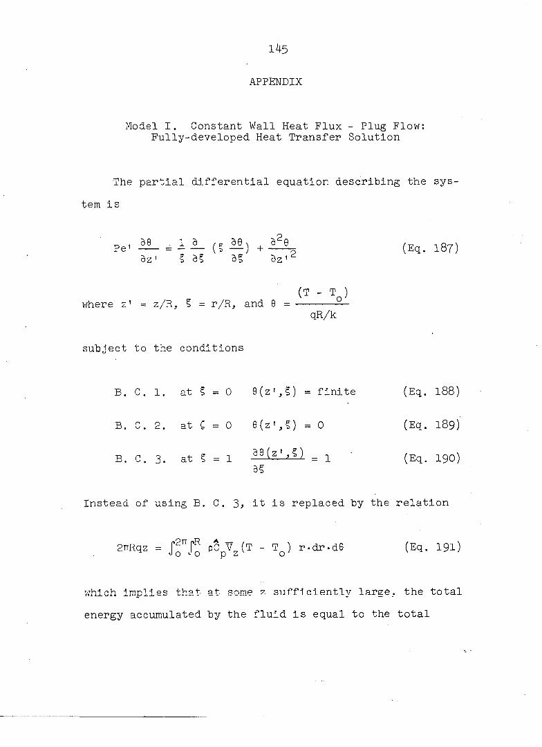
145

APPENDIX

Model I. Constant Wall Heat Flux - Plug Flow: Fully-developed Heat Transfer Solution

The partial differential equation describing the sys­

tem is

Pe' — = - — (I — ) + (Eq. 187) ÔZ' § d§ Sz '

(T - T ) where z' = z/R, § = r/R, and o

qR/k

subject to the conditions

B. C. 1. at § = 0 6(z1,1) = finite (Eq. 188)

B. C. 2. at G = 0 @(z',S) = 0 (Eq. 189)

B . C . 3 . a t § = 1 5 9 ( Z ' = 1 ( E q . 190) 9§

Instead of using B. C. 3, it is replaced by the relation

2nRqz = pCpV%(T - Tj r-dr-dG (Eq. 19l)

which implies that at some 7. sufficiently large, the total

energy accumulated by the fluid is equal to the total

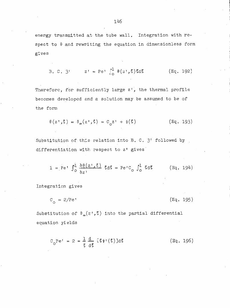
146

energy transmitted at the tube wall. Integration with re­

spect to 0 and rewriting the equation in dimensionless form

gives

B. C. 3' Z' = Pe' r 8(z',S)5d§ (Eq. 192)

Therefore, for sufficiently large z1, the thermal profile

becomes developed and a solution may be assumed to be of

the form

G(z',5) = G=(z',5) = C^z' + $(5) (Eq. 193:

Substitution of this relation into B. C. 31 followed by

differentiation with respect to z1 gives

1 = Pe' f1 59(z ' §d§ = Pe1C f1 §d§ (Eq. 194) Jo o Jo

Integration gives

= 2/Pe' (Eq. 195)

Substitution of 0œ(z',§) into the partial differential

equation yields

C Pe' = 2 = - — [§i|r' (§)]d§ ° § d§

(Eq. 196)

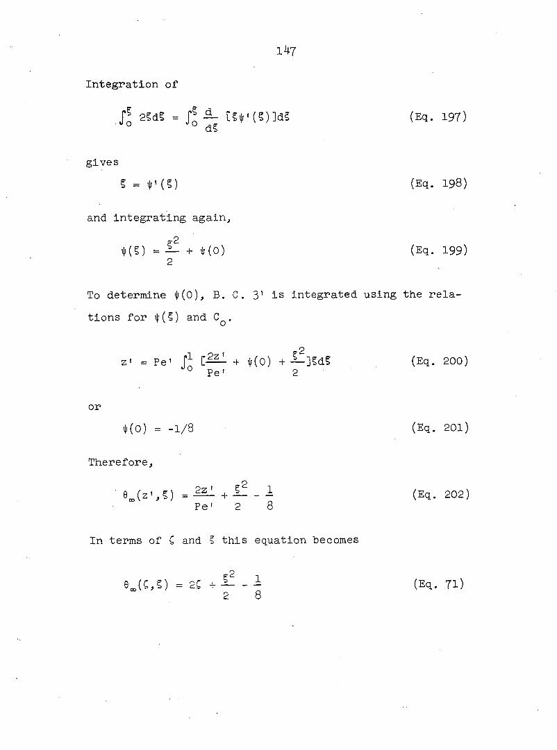
147

Integration of

fQ 2§dS = Jo [5*'(§)]d5 (Eq. 197)

gives

§ = f(?) (Eq. 198)

and integrating again,

f2 *(§) = — + MO) (Eq. 199)

2

To determine |f(0), B. C. 3' is integrated using the rela­

tions for $(§) and C .

2 21 = Pe' r1 + Ko) + —]§d§ (Eq. 200)

0 Pe' 2

or

i|i(0) = -1/8 (Eq. 201)

Therefore,

2 G.(z',5) = — +— -- (Eq. 202)

Pe' 2 8

In terms of Ç and § this equation becomes

e„(C,S) = 2ç + IÎ - -1 2 8

(Eq. 71)

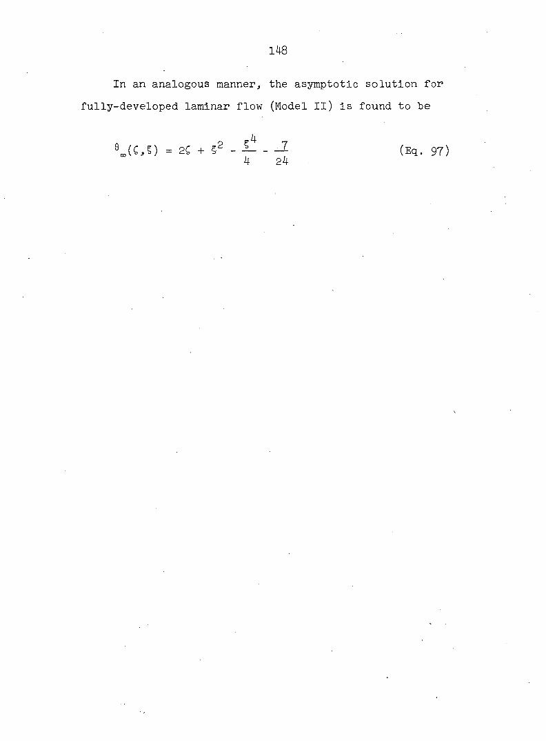
148

In an analogous manner,

fully-developed laminar flow

9JC,5) = 2C + §2 - -4

the asymptotic solution for

(Model II) is found to "be

— (Eq. 97) 24

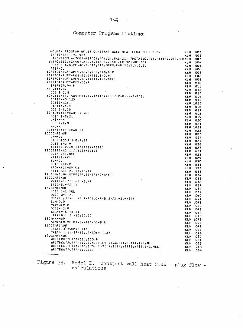
14g

Computer Program Listings

K C L M A N P R O G R A M N C I . 2 7 C O N S T A N T W A L L H E A T F L U X P L U G F L O W K L H 0 0 1 S E P T E M B E R 1 9 , 1 9 6 3 K L H 0 0 2 O I M E N S I O N A ( 7 C 0 I , B ( 7 : C I , A C ( 3 2 1 , R A U ( 2 1 I . T H E T A ( 4 0 , 2 1 I , F T A ( 4 0 , 2 1 1 , O O E K L H 0 0 3

1 V ( 4 0 , 2 1 ) , Y Z ( 4 0 I , X ( 4 C ) , Y ( 4 ' : ) , Z ( 4 0 ) , E V ( 3 2 I , B C ( 3 2 I K L H 0 0 4 C C M P O N A , B , E C , A C , T H F T A , E T A , O n E V , R A D , Y Z , X , Y , Z , E V K L H 0 0 5 A ( 1 1 = 0 . K L H 0 0 6

1 C R E A C I N P L T T A P E 5 , 5 C , M , \ E L , P A N , M P K L H 0 0 7 2 0 « E A D I N P U r T A P E 5 , 5 1 , ( A ( I ) , I = 2 , P ) K L H C 0 8 3 0 R E A C 1 N P U T T A P E 5 . 5 2 , ( X ( I ) , 1 = 1 , N E L ) K L H 0 0 9 4 0 R E A C 1 N P U T T A P E 5 , 5 3 , P K L H 0 1 C I F ( P ) 9 9 , 9 9 , 5 K L H O i l

5 0 E V I 1 ) = 0 . K L H 0 1 2 D C 6 1 = 2 , M K L H 0 1 3

6 0 E V I I I * ( I . - S C R T F I 1 - + 4 . • A ( I ) » A ( I ) / ( P » P ) ) ) » P » P / 2 . K L H 0 1 4 A C 1 1 1 = — 0 . 1 2 5 K L H 0 1 5 B C ( 1 I = A C ( 1 ) K L H 1 0 1 5 R A D t 1 ) = 1 . 0 K L H 0 1 6 0 C 7 1 = 1 , 2 0 K L H 0 1 7

7 0 R A D I I t 1 ) = R A C ( 1 ) - . 0 5 K L H 0 1 8 D C 1 0 1 = 2 , 2 1 K L H 0 1 9 J = l » M - M K L H 0 2 0 C C 8 K = 1 , M K L H 0 2 1 N = J + K K L H 1 0 2 1

8 0 A ( N ) = A ( K ) » R A O ( I ) K L H 0 2 2 1 C 0 C C N T I N U E K L H 0 2 3

J = M » 2 1 K L H 0 2 4 C A L L B E S S J I J , 0 , A , B ) K L H 0 2 5 D C 1 1 1 = 2 , M K L H 0 2 6 A C 1 I I = - 2 . » 9 I I I / ( A ( I ) » A ( I ) ) K L H 0 2 7

1 1 C 0 C I I » = A C I I ) / ( B < I ) » B < I ) ) K L H 0 2 7 C C 1 4 1 = 1 , N E L K L H 0 2 8 Y I I ) = 2 . » X ( I ) K L H 0 2 9 S l M = 0 . K L H 0 3 0 U C 1 3 K = 7 , M K L H 0 3 1 A R G = X ( I I • E V ( K ) K L H 0 3 2 I F I A R G + 1 1 2 . ) 1 3 , 1 3 , 1 2 K L H 0 3 3

1 2 5 l . M = S L M * ( E X P F ( A R ( , ) | / ( A ( K ) « A ( K ) > K L H 0 3 4 1 3 0 C C N T I N U E ( K L H 0 3 5

Y Z ( I I = 1 . / ( 1 , - e . « S I M ) K L H 0 3 6 Z ( I 1 = 8 . » Y Z ( ! ) K L H 0 3 7

1 4 C C C N T I N U E K L H 0 3 8 C C 1 7 1 = 1 , N E L K L H 0 3 9 U C 1 7 J = 1 , 2 1 K L H C 4 C O U E V I 1 , J ) = - l . , / 8 . + H A n ( J ) « R A D ( J ) / 2 . * 2 . » X ( I > K L H 0 4 1 S L M = 0 • 0 K L H 1 0 4 1 " A P = J » M - M K L H 0 4 2 O C 1 6 K = 2 , M K L H 0 4 3 A H G = E V ( K | . X ( I ) K L H 0 4 4 I F ( A R G + 1 12 . ) 11 , 1 6 , 1 5 K L H 0 4 5

1 5 C N = K + M A P K L H 1 C 4 5 S L M = S L M + B C ( K > » E X P F ( A K G ) » B ( N ) K L H C 4 6

1 6 0 C f \ T I N U F K L H 0 4 7 E T A ( I , J I = S U f * B C ( 1 ) K L H 0 4 8 T H E T A ( I , J ) = E T A ( I , J I + C D E V ! I , J ) K L H 0 4 9

1 7 0 C C N T I N U E K L H 0 5 0 H R 1 T E 0 U T P U T T A P E 1 C , 2 0 5 , P K L H 0 5 1 W R I T E C U T P u r T A P E I C , 1 7 5 , ( I , E V ( I ) , A C ( I ) , B C ( I ) , I = l , « ) K L H 0 5 2 W R I T E C U T P U T T A P E 1 C . 1 7 9 , ( I , * ( I ) , Z ( I I , Y Z ( I I , Y ( I I , I = 1 , N E L I K L H 0 5 3 W R I T E 0 U T P U T T A P E 1 C . 1 8 C K L H 0 5 4

Figure 33. Model I. Constant wall heat flux - plug flow -calculations

150

W R I T E 0 U T P U T T A P E 1 C . 1 8 1 K L H 0 5 5 D C 5 7 K * 1 » N E L K L H 0 5 6

5 7 0 W R I T E C U T P U T T A P E 1 C , 1 8 2 , X I K ) , T H E T A ( K , 1 ) , E T A I K , 1 ) , C 0 E V I K , 1 ) , T H E T A I K , 2 K L H 0 5 7 1 ) , . E T A I K , 2 ) , O O E V I K , 2 ) K L H 0 5 8

W R I T E C U T P U T T A P E 1 C . 1 8 3 K L H 0 5 9 W R I T E G U T P U T T A F f c l C , l 8 1 K L H 0 6 0 D C 5 8 K = 1 , N E L K L H 0 6 1

5 8 0 W R I T E C U T P U T T A P E I O , 1 8 2 . X I K ) , T H E T A ( K , 3 ) , E T A ( K , 3 ) , O D E V t K , 3 ) , T H E T A I K , 4 K L H 0 6 2 1 ) , E T A I K , 4 ) , O O E V I K , 4 ) K L H 0 6 3

W R I T E C U T P U T T A P E 1 0 . 1 8 4 K L H 0 6 4 W R I T E 0 U T P U T T A P E 1 C . 1 8 1 K L H 0 6 5 D C 5 9 K = 1 , N E L K L H 0 6 6

5 9 0 W R 1 T E 0 U T P U T T A P E 1 0 , 1 8 2 , X I K ) , T H E T A I K , 5 ) , E T A 1 K , 5 ) , C D E V I K , 5 ) , T H E T A I K , 6 K L H 0 6 7 1 ) , E T A I K , 6 ) , O O E V I K , 6 ) K L H 0 6 8

W R I T E 0 U T P U T T A P E 1 C , 1 8 5 K L H 0 6 9 W R I T E 0 U T P U T T A P E 1 0 . 1 8 1 K L H 0 7 0 D C 6 0 K = 1 , N E L K L H 0 7 1

6 C C H R I T E C U T P U T T A P E 1 0 , 1 8 2 , X ( K ) , T h E T A ( K , 7 ) , E T A ( K , 7 ) , c n E V I K , 7 ) , T H E T A I K , 8 K L H 0 7 2 1 ) , E T A ( K , 8 ) , 0 D E V I K , 8 I K L H 0 7 3

W R I T E 0 U T P U T T A P E 1 0 . 1 6 6 K L H 0 7 4 W R I T E 0 U T P U T T A P E 1 G , 1 8 1 K L H 0 7 5 D C 6 1 K = 1 , N E L K L H C 7 6

6 1 0 W R I T E C U T P U T T A P E 1 C , 1 8 2 . X I K ) , T h E T A I K , S > , E T A ( K , 9 ) , O D E V I K , 9 ) . T H E T A I K , 1 K L H 0 7 7 1 0 ) . E T A ( K , 1 0 1 , C O E V ( K , 1 0 1 K L H 0 7 8

W R I T E C U T P U T T A P E 1 C . 1 8 7 K L H 0 7 9 W R I T E 0 U T P U T T A P E 1 C , 1 8 1 K L H 0 8 0 nC62 K = 1 » N E L K L H 0 8 1

6 2 0 h P I T E C U T P U T T A P E l G , l 8 2 , X l K ) , T h E T A ( K , l l ) , E T A ( K , U I , O D E V ( K , 1 1 ) , T H E T A I K L H 0 8 2 1 K , 1 2 ) , E T A ( K , 1 2 ) , 0 C E V ( K , 1 2 ) K L H 0 8 3

W R I T E C U T P U T T A F E 1 C , 1 8 6 K L H 0 8 4 W H I T E C U T P U T T A P E l C . l t i l K L H 0 8 5 D C 6 3 K - 1 , N E L K L H 0 8 6

6 3 0 W R I T E U U Î P U T T A P E 1 C , 1 8 2 , X ( K ) , r H E T A ( K , 1 3 l , E T A ( K , l 3 ) , C D E V ( K , 1 3 ) , T H E T A I K L H 0 8 7 I K , 1 4 ) , E T A I K , 1 4 ) , C U E V ( K , 1 4 1 K L H 0 8 8

W R I T E Û U T P U T T A P E I C . 1 8 9 K L H 0 8 9 W R 1 T E C U T P U T T A P E 1 G , 1 8 1 K L H 0 9 0 C C 6 4 K = 1 , N E L K L H 0 9 1

6 4 C w R l T E C U T P U T T A F E l C , 1 8 2 , X ( K ) , T h E T A I K , 1 5 ) , E T A I K , 1 5 ) , O D E V ( K , 1 5 ) , T H F T A 1 K L H 0 9 2 l K , 1 6 ) , E T A ( K , l f c ) , U i ; E V ( K , 1 6 ) K L H 0 9 3

V i R I T E C U T P U T T . A P E l C , 1 9 0 K L H 0 9 4 W R I T E C U T P U T T A P E I O , 1 8 1 K L H 0 9 5 C C 6 5 K = 1 , N E L K L H 0 9 6

6 5 C c i P I T c C U T P U T T A P E l C , 1 8 2 . X ( K ) , T H E T A I K , 1 7 ) , E T A ( K , 1 7 1 . 0 D Ë V I K , 1 7 ) , T H F T A I K L H 0 9 7 1 K , 1 8 ) , E T A ( K , 1 8 ) , Ù C E V ( K , 1 8 ) K L H 0 9 8

N R I T E C U T P U T T A P E 1 C , 1 9 1 K L H 0 9 9 W K I T t C U T P U T T A P E l O , 1 8 1 K L H 1 0 0 D C 6 6 K = 1 , N E L K L H 1 0 1

6 6 0 V . R I T c C U T P U T T A P E 1 0 , 1 8 2 , X ( K ) , T H E T A I K , 1 9 ) , E T A I K , 1 9 ) , C D E V I K , 1 9 ) . T H E T A I K L H 1 0 2 1 K , 2 C ) , E T A ( K , 2 C ) , C C E V ( K , 2 0 ) K L H 1 0 3

W R I T t C U T P U T T A P F 1 C , 1 9 2 K L H 1 0 4 h R I T E C U T P l J T T A P E l C , 1 9 3 K L H 1 0 5 H C 6 7 K = 1 , N E L K L H 1 0 6

6 7 C W R I T E C U T P U T T A P E l C , 1 9 4 , X t K ) , T H E T A I K , 2 1 ) , E T A t K , 2 1 ) , C D E V I K , , 2 1 ) K L H 1 0 7 W R I T E C U T P U T T A P E 1 0 . 2 C 0 K L H 1 3 8

5 C 0 F C R V A 1 ( 4 1 2 ) K L H 1 0 9 5 1 0 F C R f A T I 3 F 1 0 . 7 , 4 F l C . 6 / 7 F 1 0 . 6 / 7 F 1 0 . 6 / 7 F l C . 6 / 3 F 1 0 . 6 ) K L H 1 1 0 5 2 C F C R ^ A T ( 4 E 1 5 . 8 ) K L H 1 1 2 5 3 C F ( . R f A T ( F 1 0 . 2 ) K L H 1 1 3

1 7 5 0 F C R f A I ( 3 H M E I G E N V A L U E E X P A N S I O N C O E F F I C I E N T T O T A L C O E F K L H 1 1 4 l F I C I E N T / t I 5 , t l 7 . 8 , 2 E 2 C . 8 > ) K L H 1 1 5

1 7 9 0 F O R M A T I f l 4 M I Z E T A L C C A L N L ' S S E L T N C . N U . I C C A L / N U . F U L L Y K L H 1 1 6 1 - U E V L L O P F n y i [ X t ( : - M E A N T H ^ T A , / ( I 4 , 2 E 1 7 . 8 , 2 E 2 3 . 8 ) ) K L H 1 1 7

Figure 33. (Continued)

151

1 8 0 C F C R M A T I l H 0 , 3 8 X 9 h P S I = 1 . 0 0 , 2 6 X 9 H P S I = 0 . 9 5 ) K L H 1 8 2 C F G R M A T ( 1 H , 7 6 1 7 . 8 ) K L H 1 8 3 C F C R M A T I 1 H 0 . 3 8 X 9 F P S I = 0 . 9 0 , 2 6 X S H P S I = 0 . 8 5 ) K L H 1 8 4 0 F C R M A T I 1 H 0 , 3 8 X 9 H P S I = C . 8 0 , 2 6 X 9 H P S I = 0 . 7 5 ) K L H 1 8 5 0 F C R M A T I 1 H 0 , 3 8 X 9 H P S I = 0 , 7 0 , 2 6 X 9 H P S I = 0 . 6 5 ) K L H 1 8 6 C F C R K A I ( 1 H 0 , 3 8 X 9 F P S I = 0 . 6 0 , 2 6 X S H P S I = C . 5 5 ) K L H 1 8 7 0 F C R M A T I l H 0 » 3 8 X 9 h P S 1 = 0 . 5 0 , 2 6 X S H P S I = 0 . 4 5 ) K L H 1 8 8 0 F C R M A T ( 1 H 0 , 3 8 X 9 H P S I = 0 . 4 0 , 2 6 X 9 H P S l = 0 . 3 5 ) K L H 1 8 9 C F O R M A T I 1 H 0 , 3 8 X 9 H P S I = C . 3 0 , 2 6 X 9 H P S I = 0 . 2 5 ) K L H l 9 0 C F C R M A T t l H 0 , 3 8 X 9 h P S I = C . 2 0 , 2 6 X S H P S I = 0 . 1 5 ) K L H 1 9 1 C F C R M A 1 ( 1 H 0 . 3 8 X 9 H P S I = C . 1 0 , 2 6 X S H P S I = C - 0 5 > K L H 1 9 2 0 F C R M A T ( 1 H 0 , 3 8 X 9 H P S l = C . O O J K L H 1 9 3 0 F C R M A T ( 6 7 H 0 Z E T A T H E T A T H E T A - D T H E K L H

1 T A - I N F I N I T Y ) . K L H 1 9 4 0 F C R M A T ( 1 H , 4 E 1 7 . 8 ) K L H 1 8 1 0 F O R Ç A T ( 1 1 6 H 0 Z E T A T H E T A T H E T A - 0 T H K L H

1 E T A - I N F I N Î T Y T H E T A T H E T A - 0 T H E T A - I N F I N 1 T Y ) K L H 2 0 C Q F C R P A T ( 3 1 H O E N D O F P R O G R A M N C . 2 7 F O R P E C = , F 9 . 2 ) K L H 2 0 5 0 F C R M A T I 3 1 H 1 H 0 L M A N P R O G R A M N O . 2 7 9 - 1 9 - 6 3 C O N S T A N T H E A T F L U X P L U G F L K L H

l O h W I T H P E C = P E C L E T N 0 . / 2 = , F 9 . 2 ) K L H G C T 0 4 K L H

9 9 0 C C N T I N U E K L H G C T O 1 7 5 , 8 5 ) , N I P K L H

7 5 0 W R I T E C U T P U T T A P E 1 0 , 2 2 5 K L H 2 2 5 0 F O R M A T ( 3 4 H 1 M X = A R G U M E N T J - Z E R O ( X ) ) K L . H

J = M « 2 1 K L H W R 1 T E C U T P U T T A P E 1 C . 2 2 6 , ( I , A t I I , B ( I ) , I = 1 , J ) K L H

2 2 6 0 F C R M A T I 1 H , 1 5 , 2 6 1 6 . 8 ) K L H 8 5 C S T 0 P 8 8 K L H

E N D K L H

118 119 120 121 122 123 124 125 126 127 128 129 130 131 132 133 134 135 136 137 138 139 139 140 141 143 144 145 146 147

Figure 33. (Continued)

152

H C L K A N P R O G R A M N O . 2 4 C A L C . E I G E N V A L U E S - C O E F F I C I E N T S S E P T . 7 , 1 9 6 3 K L H 0 0 1 C O N S T A N T W A L L H E A T F L I X K L H C O Z D I M E N S I O N A ( 3 2 ) , E ( 3 2 ) , E ( 2 C ) , C L A D ( 3 2 ) , « ( 3 2 , 3 2 ) , C ( 2 0 , 3 2 ) , T 1 2 0 . 3 2 ) , O F K L H C 0 3

1 V ( 2 C ) , A E ( 2 0 , 2 C ) , B E ( 2 C , 2 0 ) , V ( 2 C ) , V Y ( 2 0 I , I N D E X 1 I 2 C ) , I N D E X 2 I 2 0 ) , V 6 R ( 2 K L H 0 0 4 2 0 l , C L A S t 2 0 ) , I P I V O T ( 2 0 ) , P I V O T ( 2 C ) , E V t 2 C ) K L H 0 0 5

C C M K C h A , B , E , C U A C , R , C , T , D E V , A t , B E , V , V Y . V A R • C L A S . E V K L H 0 0 6 J A B = 0 K L H C 0 7

5 4 C R E A C I N P U T T A P E 5 , 5 6 , M , N , L , J E L , M A N . N A M E , D K L H 0 0 8 I F I M - J A 9 I 1 0 , I C , 1 K L H 009

I C A ( 1 ) = C . K L H C 1 C R E A D I N P U T T A P E 5 , 5 5 , ( A 1 I ) , I = 2 , M ) K L H O i l

5 5 0 F C R M A T ( 3 F 1 0 . 7 , 4 F 1 C . 6 / 7 F 1 0 . 6 / 7 F 1 C . 6 / 7 F 1 0 . 6 / 3 F 1 C . 6 1 K L H 0 1 2 5 6 0 F C R M A T ( 6 I 2 t F 7 . 2 ) K L H 0 1 3

C A L L B E S S J I M . O , A , B ) K L H 0 1 4 D C 4 1 = 1 , M K L H 0 1 5 C C 4 J = 1 , M K L H 0 1 6 I F ( I-J ) 3 , 2 , 3 K L H 0 1 7

2 C R 1 I , I ) * 0 . K L H 0 1 8 G C T C 4 K L H 0 1 9

3 0 R { I , J ) = 4 . » D » B ( J ) • ( A ( I ) » A ( I ) + A ( J ) » A ( J ) ) / ( B ( I ) » ( A ( J > » A ( J I - A ( I ) » A ( I ) I K L H 0 2 0 l » ( A I J ) > A t J > - A 1 1 ) » A I I ) ) ) K L H 0 2 1

4 0 C C N T I M J E K L H 0 2 2 1 C C R E A D I N P U T T A P E 5 . 5 7 . P K L H 0 2 3

I F ( P ) 5 4 , 9 9 , 1 1 K L H 0 2 4 1 1 C W R I T E C U T P U T T A P E 1 C , 5 C , P K L H 0 2 5 5 C 0 F C R M A T I 7 9 H 1 I - 0 1 M A N P R O G R A M N O . 2 4 O F 7 S E P T . 1 9 6 3 - C A L C . E I G E N V A L U E S A N K L H 3 2 6

I D C O E F F I C I E N T S F O R P E C = , F 8 . 2 ) K L H K L H

0 2 7 0 2 8

C A L C U L A T E I N I T I A L E S T I M A T E S O F A S S O C I A T E D C O E F F . A N D F I G E N V A L U E S K L H 0 2 9 K L H C3C

D C 1 2 1 = 2 , N K L H 0 3 1 1 2 0 E l I M l D / 3 . - S O R T F ( ( D / 3 . ) » ( C / 3 . ) * A t I ) » A ( I ) / { P » P ) ) ) » P » P K L H 0 3 2

E ( 1 ) = C . K L H 033 C C 1 5 1 = 2 , N K L H 0 3 4 C G I 5 J = 2 , M K L H 0 3 5 I F ( I - J ) 1 3 , 1 4 , 1 3 K L H 0 3 6

1 3 C C I I , J ) = - E ( I ) * R ( I , J 1 / ( E ( I > • E t I ) / ( P ' P ) - 2 . » C » E ( I 1 / 3 . - A I J ) > A t J ) ) K L H 0 3 7 G L T C l b K L H 038

1 4 0 C I I , I ) = 1 . C K L H 039 1 5 C C C N T I N U E K L H C 4 C

C C 1 6 1 = 2 , N K L H 041 1 6 0 C I I , L ) = - R ( 1 , I ) / ( 1 1 I ) / t P » P > - 0 / 2 . ) K L H 0 4 2

C C 7 5 J = 2 , M K L H 0 4 3 7 5 C C 1 I , J ) = 0 . K L H 0 4 4

C I 1 , 1 ) = 1 . 0 K L H K L H

0 4 5 0 4 6

C C M P U I A T I O N - I T E R A T I O N F O R E I G E N V A L U E S - A S S O C I A T E D C O E F F I C I E N T S K L H 0 4 7 K L H 0 4 8

K = 1 K L H 0 4 9 1 7 0 K = K t l K L H 0 5 0

N E B = 0 K L H 0 5 1 1 8 C C C 2 4 1 = 1 , M K L H 0 5 2

1 F ( I - I ) 6 0 , M » 6 0 K L H 0 5 3 6 C 0 C l A D ( I ) = E ( K ) » E ( K > / ! P » P ) - 2 . , » D » E ( K I / 3 . - A t I ) < • A t I ) K L H C 5 4

G C T G 1 S K L H 0 5 5 6 1 0 Q L A C ( l ) = E ( K ) s E ( K ) / ( P * P ) - O E ( K ) / 2 . K L H 0 5 6 1 9 C I F ( K - I ) 2 1 , 2 C , 2 1 - K L H 0 5 7 2 C 0 C I K , 1 1 = 1 . 0 K L H 0 5 8

G C T C 2 4 K L H 0 5 9 2 1 0 S U M = 0 . K L H G 6 C

C L 2 3 J = 1 , M K L H 0 6 1

Figure 34. Model II. Constant wall heat flux - fully-developed laminar flow - calculation of eigenvalues and coefficients

153

I F 1 I - J > 2 2 , 2 3 , 2 2 K L H 0 6 2 2 2 0 S U M = S L M * R ( I , J ) « C ( K , J ) K L H 0 6 3 2 3 0 C C N T I N U E K L H 0 6 4

C C K , l ) = - S U M « E I K ) / C U A D ( I l K L H 0 6 5 T ( K , I > = S U M K L H 0 6 6

2 4 C C C N T I N U E K L H 0 6 7 S U M = 0 . K L H 0 6 7 0 0 3 0 1 = 1 , M K L H 0 6 8 I F C K - I 1 2 9 , 3 0 , 2 9 K L H 0 6 9

2 9 0 S U M = S U M + R ( K , I ) » C ( K , I ) K L H 0 7 0 3 0 C C C N T I N U E K L H 0 7 1

T ( K , K ) = S U M K L H 0 7 2 D E V ( K ) = Q U A D ( K ) + T t K , K ) » E ( K ) K L H 0 7 3 E V ( K ) = ( 2 . * D / 3 . - S U M - S C R T F 1 ( 2 . « 0 / 3 . - S I M ) • ( 2 . « 0 / 3 . - S U M ) - I - 4 . • A ( K ) * A ( K ) / K L H 0 7 4

1 ( P » P ) ) ) * P * P / 2 . K L H 0 7 5 J A B = M K L H 0 7 6 I F ( N A M E ) 1 3 0 , 1 2 0 , 1 2 0 K L H 0 7 7

1 2 0 0 W R I T E C U T P U T T A P E 1 0 , 1 2 5 , K , 0 U A 0 ( K ) , T ( K , K ) , D E V I K ) , E ( K ) , E V ( K ) K L H 0 7 8 1 2 5 0 F C R M A T ( 8 6 H 0 M Q U A D R A T I C S O P A T I C N D E V I A T I O N E K L H 0 7 9

1 I G E N V A L U E R E C A L C . E I G E N V A L L E / ( I A . 5 E 1 6 . 8 I 1 K L H C 8 0 W R I T E C U T P U T T A P E 1 0 . 1 2 6 , ( J , C ( K , J ) , J = 1 , M ) K L H 0 8 1

1 2 6 0 F 0 R M A T ( 3 0 H J A S S O C I A T E D C O E F F I C I E N T / 1 1 4 , E 1 7 . 8 ) I K L H 0 8 2 1 3 0 0 N E B = N E B * 1 K L H 1 8 2

E ( K I = E V I K ) K L H 3 8 2 I F 1 N E E — L > 1 8 * 3 1 * 3 1 K L H 4 8 2

3 1 0 I F C K - N > 1 7 , 1 3 1 , 1 3 1 K L H 5 8 2 1 3 1 C W R I T E C U T P U T T A P E 1 C , 1 2 7 , ( I , E U ) , I = 1 , N ) K L H 6 8 2 1 2 7 0 F O R M A T ( 1 8 H H E I G E N V A L U E / 1 1 4 , E 1 6 . 8 ) > K L H 7 8 2

H R 1 T E C U T P U T T A P E 1 0 , 1 7 5 K L H 8 8 2 1 7 5 0 F 0 R M A T ( 1 H 0 . 2 0 X 2 4 H A S S O C I A T E D C O E F F I C I E N T S ) K L H 9 8 2

W R I T E C U T P U T T A P E 1 C . 7 6 K L H 0 8 3 7 6 0 F O R M A T ( 1 O 9 H 0 I M = 1 M = 2 M = 3 K L H 0 8 4

1 M = 4 M = 5 , M = 6 M = 7 ) K L H 0 8 5 0 0 3 3 J = 1 , M K L H 0 8 6

3 3 0 W R I T E U U T P U T T A P E 1 0 , 1 0 0 , J , ( C I K , J ) , K = 1 , 7 ) K L H 0 8 7 W R I T E G U T P U T T A P E 1 C . 7 7 K L H 0 8 8

1 C O O F C R K A T ( 1 H , I 3 . 7 E 1 6 . 8 ) K L H 0 8 9 7 7 0 F C R M A T ( 1 1 0 H C I M = 8 M = 9 M = 1 0 K L H 0 9 0

1 M = 1 1 M = 1 2 M = 1 3 M = 1 4 ) K L H 0 9 1 0 0 3 4 J = 1 , M K L H 0 9 2

3 4 0 K R I T E C U T P U T T A P E 1 C , 1 0 0 , J , ( C t K , J ) , K = 8 , 1 4 ) K L H 0 9 3 W R I T E O U T P U T T A P E 1 C . 7 8 K L H 0 9 4

7 8 C F C R V A T I 9 5 H 0 I M = 1 5 f « 1 6 M = 1 7 K L H 0 9 5 1 M = 1 8 M = 1 9 M = 2 0 ) K L H 0 9 6

0 0 3 5 J = 1 , M K L H 0 9 7 • 3 5 C W R I T E C U T P U T T A P E 1 C , 1 0 1 , J , ( C ( K , J ) , K = 1 5 , 2 0 ) K L H 0 9 8 1 0 1 C F C R M A T ( 1 H , I 3 , 6 E 1 6 . 8 ) K L H C 9 9

K L H 1 0 0 D E T E R M I N A T I O N O F E X P A N S I O N C O E F F I C I E N T S K L H 1 0 1

M E T H O D 1 = C L A S S I C A L T E C H N I Q U E K L H 1 0 2 K L H 1 0 3

I F ( J E L ) 4 2 , 4 2 , 3 6 K L H 1 0 4 3 6 C C C 3 7 1 = 1 , N K L H 1 0 5

C C 3 7 J = 1 , N K L H 1 0 6 3 7 C A E I I , J I = C ( J , I ) / ( B ( J ) » B ( J 1 ) K L H 1 0 7

V ( 1 ) = — 1 . / 1 6 . K L H 1 0 8 D C 3 8 1 = 2 , N K L H 1 0 9

3 8 C V ( I ) = - ( A ( I ) » A ( I ) + 8 . ) / ( B ( I ) » ( A ( I ) » » 4 . ) ) K L H 1 1 0 w k I T c C U T P U T T A P E l C , 8 0 K L H 1 1 1

8 0 C F C R M A T I 4 6 H O C O E F F . M A T R I X - N O N H O M O . V E C T O R - C L A S S I C A L M E T H O D ) K L H 1 1 2

Figure 3^. (Continued)

t

t

154

W R I T E C U T P U T T A P E 1 C . 7 6 D C 3 9 1 - 1 , N

3 9 0 W R I T E C U T P U T T A P E 1 C » 1 0 0 , I , ( A E I I « J ) , J * 1 , 7 ) H R I T E C U T P U T T A P E 1 0 . 7 7 D C 4 C I - l . N

4 0 0 W R I T E G U T P U T T A P E 1 0 , 1 0 0 , I , I A E ( I , J ) , J = 8 , 1 4 ) W R I T E C U T P V T T A P E 1 0 . 8 1

8 1 0 F C R M A T { 1 1 7 H 0 I M = 1 5 M = 1 6 M = 1 7 1 M = 1 9 M = 2 0 N O N - H C K O . V E C T O R !

0 0 4 1 I - l . N 4 1 0 W R I T E C U T P U T T A P E 1 0 , 1 0 0 , I , I A E t I , J I , J = 1 5 , 2 0 ) , V ( I )

C A L L M A T I N V I A E . N , V , 2 0 , 1 . D E T E R f , I N D E X I , I N D E X 2 , I P I V O T , P I V O T ) 4 2 0 C C N T I N U 6

I F ( M A N ) 5 2 , 5 2 , 4 3 4 3 0 D C 4 4 1 = 1 , N

B E l l , l ) » C I I , l ) / t B ( I ) » B ( I ) ) 4 4 C 8 E I I , 1 ) » C ( I , 1 )

0046 1-2,N D C 4 6 J = 2 , N SUM=0. D C 4 5 L - l , M

4 5 0 S U M * S t M + C ( I , L I * C ( J , L ) » B ( L ) » 8 ( L ! 4 6 0 B E I I , J ) = S U M / ( 8 1 J ) * B I J ) )

0 C 4 6 1 = 2 , N S L M - O . D C 4 7 J = 2 , M

4 7 0 S L H - S I M * C ( I , J ) » 8 ( J ) » ( A ( J ) » A t J ! + 0 . ) / ( A < J ) » » 4 . ) 4 8 0 V Y I I > = - S U M - ( C ( l , l ) / 1 6 . )

V Y ( 1 ) = - 1 . / 1 6 . W R I T E C U T P U T T A P E 1 G . 8 2

8 2 0 F C R M A T I 4 8 H O C O E F F . M A T R I X - N O N H O M O . V E C T C R - V A R I A T 1 0 N A L M E T H O D ) W R I T E C U T P U T T A P E 1 0 . 7 6 D C 4 9 1 = 1 , N

4 9 0 W R I T E 0 U T P U T T A P E 1 0 , I O C , I , ( B E I I , J ) , J = 1 , 7 1 W R I T E C U T P U T T A P E 1 0 . 7 7 D C 9 0 1 = 1 , N

9 0 0 W R I T E C U T P U T T A P E 1 0 , 1 0 0 , I , ( B E ( I , J ) , J = 8 , 1 4 ) W R I T E C U T P U T T A P E 1 0 . 8 1 0 0 5 1 1 = 1 , N

S I O H R I T E C U T P U T T A P I U O . I O O . I , I B E l I , J ) , J = 1 5 , 2 0 ) , V Y ( I ) C A L L M A T I N V I B E . N , V Y . 2 0 , 1 , T E R M , I N D E X 1 , I N D E X 2 , 1 P I V O T , P I V O T )

5 2 0 0 C 5 3 1 = 1 , N C L A S ( 1 I = V C I ) / ( B ( 1 1 » B ( I ) )

5 3 0 V A R C ! ) = V Y ( I ! / I B ! I ! » B ! 1 ) ! , H R I T E C U T P U T T A P E 1 0 , 8 4 , ( I , V I I ) . C L A S S I I , V Y I I ) , V A R ( I ) , I = 1 , N )

8 4 C F C R M A T ( 7 0 H M C L A S S I C A L A I M ) A I M ) / J I M ) e J I M ) V A R I A T I O N A L A I M ) l A ( M ) / J ( M ) e J ( M ) / ( I 3 , 4 E 1 6 . 8 ) )

G C T O I O 9 9 0 C C N T I N U E 5 7 0 F 0 R M A T I F 1 0 . 2 )

S T 0 P 8 S E N D

K L H 1 3 K L H 1 4 K L H 1 5 K L H 1 6 K L H 1 7 K L H 1 8 K L H 1 9 K L H 2 0 K L H 2 1 K L H 2 2 K L H 2 3 K L H 2 4 K L H 2 5 K L H 2 6 K L H 2 7 K L H 2 8 K L H 2 9 K L H 3 0 K L H 3 1 K L H 3 2 K L H 3 3 K L H 3 4 K L H 3 5 K L H 3 6 K L H 3 7 K L H 3 8 K L H 3 9 K L H 4 0 K L H 4 1 K L H 4 2 K L H 4 3 K L H 4 4 K L H 4 5 K L H 4 6 K L H 4 7 K L H 4 8 K L H 4 9 K L H 5 0 K L H 5 1 K L H 5 2 K L H 5 3 K L H 5 4 K L H 5 5 K L H 5 6 K L H 5 7 K L H 5 8 K L H 5 9 K L H 6 0 K L H 6 1 K L H 1 6 1 K L H 6 2 K L H 6 3

Figure 34. (Continued)

155

H C L M A N P R O G R A M N O . 2 8 C O N S T A N T W A L L H E A T F L U X , P A R A B O L I C V E L O C I T Y P R K L H C 0 1 O F 1 L E , F I N A L C A L C U L A T I O N S S E P T E M B E R 2 0 , 1 9 6 3 K L H C O 2 D I M E N S I O N A ( 7 C C ) , B ( 7 C C > , C ( 2 0 , 3 2 ) , E 1 2 0 ) , A C ( 2 0 ) , X ( 4 0 ) , U ( 4 0 ) , Y ( 4 v ) , C H K L H 0 0 3

1 A F R ( 2 0 , 2 1 ) , T H E T A ( 4 0 , 2 1 ) , E T A ( 4 0 , 2 1 ) , R A C ( 2 5 ) , O D E V ( 4 0 , 2 1 1 , Z ( 4 0 ) , C O E ( 2 K L H 0 0 4 2 0 ) K L H 0 0 5

C C M M O N A , B , C , T H E T A , E T A , O D E V , C F A F R , E , A C , X , Y , U , Z , R A D , C O E K L H 0 0 6 1 0 A ( 1 ) = 0 . K L H 0 0 7 2 0 R E A C I N P U T T A P E 5 , 1 5 0 , M , N E L K L H 0 0 8 3 0 R E A C I N P U T T A P E 5 , 1 5 1 , ( X ( I ) , 1 = l . N E L ) K L H 0 0 9 4 C R E A C I N P U T T A P E 5 , 1 5 2 , ( A ( I 1 , 1 = 2 » M ) K L H 0 1 0 9 C R A 0 ( 1 ) = 1 . 0 K L H O i l

1 0 0 0 C 1 1 1 = 1 , 2 0 K L H 0 1 2 1 1 0 R A D I 1 * 1 ) = R A D ( ' I I - . C 5 K L H 0 1 3

J 1 = M K L H 0 1 4 1 2 0 D C 1 5 J = 2 , 2 1 K L H 0 1 5 1 3 0 0 0 1 5 1 = 1 , M . K L H 0 1 6 1 4 0 J 1 = J 1 + 1 K L H 0 1 7 1 5 C A ( J 1 ) = R A 0 I J ) » A ( I ) K L H 0 1 8 I 6 0 C A L L B E S S J ( 6 7 2 , 0 , A , 8 I K L H 0 1 9 1 7 0 R E A C I N P U T T A P E 5 , 1 5 3 , P , L K L H 0 2 0 1 8 C I F ( P ) 9 9 , 2 , 1 9 K L H 0 2 1 1 9 0 W R I T E O U T P U T T A P E 1 0 1 2 0 5 1 P K L H 0 2 2

R E A 0 I N P U T T A P E 5 , 1 5 1 , ( E l I ) , 1 = l . L ) K L H 0 2 3 R E A C I N P U T T A P E 5 , 1 5 1 , I A C ( I ) , I = 1 , L ) K L H 0 2 4 D C 2 0 I = 1 , L K L H 0 2 5

2 0 0 R E A C I N P U T T A P E 5 , 1 5 1 , ( C I I , J ) , J = 1 , M ) K L H 0 2 6 C A L C U L A T I O N O F L O C A L N U S S E L T N U M B E R S A N D M I X E D - M E A N T H E T A K L H 0 2 7 0 C 2 5 K = 1 , N E L K L H 0 2 6 S L M T = 0 . K L H 0 2 9 D C 2 4 1 = 2 , L K L H 0 3 0 S U M = 0 . K L H 0 3 1 C C 2 1 J = 2 , M K L H 0 3 2

2 1 C S L M = S L M + C ( I , J ) • E ( J ) » ( 1 . + ( 8 . / ( A ( J ) * A ( J ) ) > ) K L H 0 3 3 C C E ( I ) = A C ( I ) * 2 . / ( Q ( I ) » B ( I ) ) K L H 0 3 4 S U M = C ( I , 1 ) - S U M K L H 0 3 5 A R G = E ( I ) « X ( K ) K L H 0 3 6 I F ( A R G + 1 1 2 . > 2 4 , 2 4 , 2 2 K L H 0 3 7

2 2 C S U M T = S U M T + C G E ( I ) • S U M • ( E X P F ( A R G ) ) / 2 . K L H 0 3 8 2 4 C C C N T I N U E K L H 0 3 9

U ( K ) = 1 . / ( ( 1 1 . / 4 8 . l - S U M T ) K L H C 4 0 2 5 C Z ( K ) = l l . * U ( K ) / 4 8 . K L H 0 4 1

0 C 3 C K = 1 , N E L K L H 0 4 2 S U M T = 2 . » ( X ( K ) * A C ( 1 ) ) K L H 0 4 3 C C 2 9 1 = 2 , L K L H 0 4 4 A R G = E ( I ) » X ( K ) K L H 0 4 5 I F I A R G + 1 1 2 . > 2 9 , 2 9 , 2 6 K L H 0 4 6

2 6 0 S L M = 0 . K L H 0 4 7 C C 2 7 J = 2 , M K L H 0 4 8

2 7 C S L M = S U M - 4 . » C ( I , J ) » B ( J ) / ( A ( J ) » A ( J ) I K L H 0 4 9 S L M = S L M + C ( 1 , 1 ) K L H 0 5 0

2 8 0 S L M T = S U M T + 2 . » C 0 E i I ) • S U M » E X P F ( A R G ) K L H 0 5 2 2 9 0 C C N T I N U E K L H 0 5 3 3 0 C Y ( K ) = S U M T K L H 0 5 4 .

C C E ( 1 ) = 2 . » A C ( 1 ) K L H 0 5 5 : 0 C 3 2 1 = 2 , L K L H 0 5 6

D C 3 2 K = l , 2 1 K L H 0 5 7 S L M = 0 . K L H 0 5 8 K Y = K » M - M K L H 0 5 9 D C 3 1 J = 1 , M K L H 0 6 0 N 1 = J * K Y K L H 0 6 1

3 1 C S L M = S U M + C ( I , J ) * e ( N l ) K L H 0 6 2

Figure 35- Model II. developed

Constant wall heat flux - fully-laminar flow - final calculations

156

3 2 0 0 A F R ( I , K ) = S U P K L H 0 6 3 D C 3 3 1 = 1 , 2 1 K L H 0 6 4

3 3 C O A F R U , l ) = l . C K L H 0 6 5 C A L C U L A T I O N O F T H E R M A L P R O F I L E S K L H 0 6 6 0 0 3 6 1 = 1 , N E L K L H 0 6 7 0 C 3 6 K = l , 2 1 K L H 0 6 8 S L M = 2 . » A C I 1 > K L H 0 6 9 0 U E V 1 r ,K ) = 2 . » X ( I ) + R A n ( K ) » R A O ( K ) - I R A C I K ) * » 4 . ) / 4 , . - 7 . / 2 4 . K L H 0 7 0 D C 3 5 J = 2 , L K L H 0 7 1 A R G = E 1 J ) * X ( I ) K L H 0 7 2 1 F ( A R G + 1 1 2 . ) 3 5 , 3 5 , 3 4 K L H 0 7 3

3 4 0 S L ! M = S U M + C O E I J ) » C H A F R ( J , K I * E X P F ( A R G ) K L H 0 7 4 3 5 0 C C N T I N U E K L H 0 7 5

E T A ( I , K ) = S U M K L H 0 7 6 3 6 0 T I - E T A I I , K ) = C D E V ( I , K ) + E T A t I , K ) K L H 0 7 7

H R I T E C U T P U T T A P E 1 C , 1 7 3 , P K L H 0 7 8 1 7 3 0 F 0 R M A T ( 8 7 H 1 O U T P U T D A T A F O R H O L M A N P R O G R A M N O . 2 8 O F S E P T E M B E R 2 0 , K L H 0 7 9

1 1 9 6 3 U S I N G P E C = P E C L E T N U M B E R / 2 = , F 9 . 2 ) K L H C 8 0 W R I T E C U T P U T T A P E 1 C , 1 7 5 , ( I , E ( I f , A C ( I ) , C C E ( I 1 , 1 = 1 , L ) K L H 0 8 1

1 7 5 0 F 0 R M A T ( 5 5 H M E I G E N V A L U E E X P A N S I O N C O E F F . 2 A ( M ) / ( 9 ( M ) » B ( M ) / K L H 0 8 2 1 . 1 I 4 . 2 E 1 7 . 8 ) ) K L H 0 8 3

H R I T E C U T P U T T A P E 1 C , 2 3 C , P K L H 0 8 4 2 3 0 0 F C R K A T I 4 2 H 0 A S S 0 C I A T E C C O E F F I C I E N T S F O R P E C L E T 1 N C . / 2 = , F 9 . 2 ) K L H 0 8 5

W R I T E O U T P U T T A P E 1 0 , 1 7 6 K L H 0 8 6 D C 3 8 J = 1 , M K L H 0 8 7

3 8 C W R I T E C U T P U T T A P E 1 G . 1 7 7 , J , I C ( I , J ) , 1 = 1 , 7 ) K L H 0 8 8 W R I T E C U T P U T T A P E I O , 1 7 8 K L H 0 8 9 D C 3 9 J = 1 , M K L H 0 9 0

3 9 C W R I T E C U T P U T T A P E 1 0 , 1 7 7 , J , ( C t I , J ) , 1 = 8 , 1 4 ) K L H 0 9 1 W R I T E C U T P U T T A P E I O , 2 3 2 K L H 0 9 2 C C 4 C J = 1 , M K L H 0 9 3

4 0 0 W R 1 T E C U T P U T T A P E 1 C , 1 7 7 , J , ( C ( I , J ) , 1 = 1 5 , 2 0 ) K L H 0 9 4 W R I T E O U T P U T T A P E 1 0 , 1 7 9 , ( I , X ( I ) , U ( I I , Z ( I ) , Y ( I ) , I = 1 . N E L ) K L H 0 9 5 W R I T E C U T P U T T A P E I O , 1 8 0 K L H 0 9 6 W R I T E C U T P U T T A P E I O , 1 8 1 K L H 0 9 7 0 C 5 7 K = 1 , N E L K L H 098

5 7 0 W R I T E C U T P U T T A P E I O , 1 8 2 , X I K ) , T H E T A ( K , 1 ) , E T A l - K , 1 ) , O D E V 1 K , 1 ) . T H E T A I K , 2 K L H 0 9 9 1 ) , E T A 1 K , 2 ) # O D E V I K , 2 ) K L H 1 0 0

W R I T E C U T P U T T A P E I O , 1 8 3 K L H 1 0 1 W R I T E C U T P U T T A P E I O , 1 8 1 K L H 1 0 2 C C 5 8 K = 1 , N E L K L H 1 0 3

5 8 C W R I T E C U T P U T T A P E 1 C , 1 8 2 , X I K ) , T H E T A I K , 3 ) . E T A I K , 3 ) . C D E V I K , 3 ) . T H E T A I K , 4 K L H 1 0 4 1 ) , E T A I K , 4 ) , 0 D E V ( K , 4 ) K L H 1 0 5

W R I T E C U T P U T T A P E I O , 1 8 4 K L H 1 0 6 W R I T E C U T P U T T A P E I O , 1 8 1 K L H 1 0 7 C C 5 9 K = 1 , N E L K L H 1 0 8

5 9 0 W R I T E C U T P U T T A P E 1 0 , 1 8 2 , X I K ) , T H E T A I K , 5 ) , E T A I K , 5 ) . C O E V I K , 5 ) , T H E T A I K , 6 K L H 1 0 9 1 ) , E T A I K , 6 ) , 0 0 E V I K , 6 ) K L H 1 1 0

W R I T E C U T P U T T A P E I O , 1 8 5 K L H 1 1 1 W R I T E Q U T P U T T A P E I O , 1 8 1 K L H 1 1 2 D C 6 0 K = 1 , N E L K L H 1 1 3

6 0 0 W R I T E C U T P U T T A P E 1 0 , 1 8 2 , X I K ) , T H E T A I K , 7 ) , E T A I K , 7 ) , 0 D E V ( K , 7 ) , T H E T A I K , 8 K L H 1 1 4 1 ) , E T A I K , 8 ) , 0 0 E V 1 K , 8 I K L H 1 1 5

W R I T E C U T P U T T A P E I O , 1 8 6 K L H 1 1 6 W R I T E C U T P U T T A P E I O , 1 8 1 K L H 1 1 7 C C 6 1 K = 1 » N E L K L H 1 1 8

6 1 C W R I T E 0 U T P U T T A P E 1 0 , 1 8 2 , X I K ) « T H E T A I K , 9 ) , E T A I K , 9 ) , C D E V I K , 9 ) , T H E T A I K , F 1 K L H 1 1 9 1 0 ) , E T A I K , 1 0 ) . C D E V I K , I C ) K L H 1 2 0

W R I T E t J U T P U T T A P E 1 0 . 1 8 7 K L H 1 2 1 W R I T E C U T P U T T A P E I O , 1 8 1 K L H 1 2 2

Figure 35. (Continued)

157

0 C 6 2 K - l . N E L K L H 1 2 3 6 2 0 W R I T E C U T P U T T A P E 1 0 , 1 8 2 , X I K ) . T H E T A I K , 1 1 ) . E T A I K , 1 1 ) , n O E V I K , l l ) , T H E T A I K L H 1 2 4

I K , 1 2 ) , E T A I K , 1 2 ) , O D E V I K , 1 2 » K L H 1 2 5 W R I T E t J U T P U T T A P E l O , 1 8 8 K L H 1 2 6 W R I T E C U T P U T T A P E I O , 1 8 1 K L H 1 2 7 0 C 6 3 K = 1 , N E L K L H 1 2 8

6 3 0 W R I T E O U T P U T T A P E 1 C , 1 8 2 , X I K ) , T H E T A I K , 1 3 ) , E T A I K , 1 3 ) . C D E V I K , 1 3 ) , T H E T A I K L H 1 2 9 I K , 1 4 ) , E T A I K , 1 4 ) , C D E V I K , 1 4 ) K L H 1 3 0

W R I T E C U T P U T T A P E I O , 1 8 9 K L H 1 3 1 W R I T E C U T P U T T A P E I O , 1 8 1 , K L H 1 3 2 D C 6 4 K = 1 » N E L K L H 1 3 3

6 4 C W R I T E C U T P U T T A P E 1 0 , 1 8 2 , X I K ) , T H E T A I K , 1 5 ) , E T A I K , 1 5 ) , C D E V I K , 1 5 ) , T H E T A I K L H 1 3 4 1 K , 1 6 ) , E T A I K , 1 6 ) , C D E V I K , 1 6 ) K L H 1 3 5

W R I T E C U T P U T T A P E I O , 1 9 C K L H 1 3 6 W R I T E C U T P U T T A P E I O , 1 8 1 K L H 1 3 7 C C 6 5 K = 1 , N E L K L H 1 3 8

6 5 C W R I T E C U T P U T T A P E I O , 1 8 2 , X I K ) , T H t T A I K , 1 7 ) , E T A I K , 1 7 ) . C n t V I K , 1 7 ) , T H E T A I K L H 1 3 9 l K t ! 8 ) , E T A I K , 1 8 1 , C D E V I K , 1 8 ) K L H 1 4 0

W R I T E C U T P U T T A P E I O , 1 9 1 K L H 1 4 1 W R I T E C U T P U T T A P E I O , 1 8 1 K L H 1 4 2 D C 6 6 K - l . N E L K L H 1 4 3

6 6 0 W R I T É C U T P U T T A P E 1 C , 1 8 2 , X I K ) , T H E T A I K , 1 9 ) , F T A I K , 1 9 ) . C D E V I K , 1 9 ) . T H E T A I K L H 1 4 4 I K , 2 0 ) , E T A I K , 2 C ) , 0 C E V ( K , 2 G ) K L H 1 4 5

W R I T E C U T P U T T A P E I O , 1 9 2 K L H 1 4 6 W R I T E C U T P U T T A P E I O , 1 9 3 K L H 1 4 7 0 C 6 7 K = 1 , N E L K L H 1 4 8

6 7 0 W R I T E C U T P U T T A P E 1 0 , 1 9 4 , X I K ) , T H E T A I K , 2 1 ) , E T A I K , 2 1 I , O D î V I K , ? l ) K L H 1 4 9 1 7 9 0 F C R M A T I 8 4 H I Z E T A L O C A L N I S S E L T N C . N L . L C C A L / N l I . F U L L Y K L H 1 5 0

l - H E V E L O P E D M I X E D - M E A N T H E T A , / 1 I 5 , 2 E 1 7 . 8 , 2 E 2 C ; . 8 ) ) K L H 1 5 1 1 8 1 C F C R M A T 1 1 1 8 H C Z E T A T H E T A f H E T A - D T H K L H 1 5 2

1 E T A - I N F I N I T Y T H E T A T H E T A - D T H f c T A - l N F I N I T Y ) K L H 1 5 3 1 8 0 0 F C R M A 1 I 1 H 0 . 3 8 X 9 H P S I = 1 . 0 0 , 2 6 X S H P S 1 = 0 . S 5 ) K L H 1 5 4 1 8 2 C F C R M A T I 1 H . 7 E 1 7 . 8 ) K L H 1 5 5 1 8 3 O F C R M A t l l H 0 , 3 8 X 9 H P S I = C . 9 0 , 2 6 X 9 H P S I = 3 . 8 5 ) K L H 1 5 6 1 8 4 C F C R P A T 1 1 H 0 . 3 8 X 9 H P S I = 0 . 6 0 , 2 6 X S H P S I = 0 . 7 5 ) K L H 1 5 7 1 8 5 C F C R M A T 1 1 H 0 . 3 8 X 9 H P S I = C . 7 C , 2 6 X S H P S l = 0 . 6 5 ) K L H 1 5 8 1 8 6 0 F C R M A T I 1 H 0 . 3 9 X 9 H P S I = C . 6 0 , ? 6 X S H P S I = 0 . 5 5 ) K L H 1 5 9 1 8 7 0 F C j R M A T 1 1 H 9 , 3 8 X 9 H P S I = C . 5 C , 2 6 X S H P S t = C . 4 5 > K L H 1 6 0 1 8 8 C F C R M A T 1 1 H C . 3 8 X 9 H P S I = 0 . 4 0 , 2 6 X 9 H P S I = 0 . 3 5 ) K L H 1 6 1 1 8 9 0 F C R M A T 1 1 H 0 . 3 8 X 9 H P S I = 0 . 3 0 , 2 6 X S H P S I = 0 . 2 5 ) K L H 1 6 2 1 9 0 C F C R M A I 1 1 H 0 . 3 8 X 9 H P S I = 0 . 2 0 , 2 6 X 9 H P S I = 0 . 1 5 ) K L H 1 6 3 1 9 1 C F C R M A T I 1 H 0 . 3 8 X 9 H P S I = C . 1 0 , 2 6 X S H P S I = 0 . 3 5 ) K L H 1 6 4 1 9 2 C F C R M A T I l H C , 3 8 X 9 h P S ! = 0 . 0 0 ) K L H 1 6 5 1 9 3 0 F C R M A I I 6 7 H 0 Z E T A T H E T A T H [ T A - r T H i i K L H 1 6 6

' 1 T A - I I N F I N I T Y ) K L H 1 6 7 1 9 4 C F C R K A T 1 1 H . 4 E 1 7 . 8 ) K L H 1 6 8

W R I T E C U T P U T T A P E 1 G . 1 9 5 , P K L H 1 6 9 W R I T E C U T P U T T A P E I O , 1 9 6 K L H 1 7 0 0 C 6 9 1 = 1 , L K L H 1 7 1

6 9 0 W R I T E C U T P U T T A P E 1 0 , 1 7 7 , I , I C H A F R I I , K ) , K = 1 , 7 ) K L H 1 7 2 W R I T E C U T P U T T A P E I O , 1 9 7 K L H 1 7 3 C C 7 0 1 = 1 . L K L H 1 7 4

6 9 C W R I T E C U T P U T T A P E 1 C . 1 7 7 , I , I C H A F R I I , K ) , K = 8 , 1 4 ) K L H 1 7 5

W R I T E C U T P U T T A P E I O , 1 9 8 K L H 1 7 6 C C 7 1 1 = 1 , L K L H 1 7 7

6 9 0 W R I T E C U T P U T T A P E 1 0 . 1 7 7 , 1 , I C H A F R I I , K ) , K = 1 5 , 2 1 ) K L H 1 7 8 W R I T E C U T P U T T A P E 1 0 , 2 0 0 K L H 1 7 9 G O T O 1 7 K L H 1 8 0

1 9 5 C F C R P A T 1 5 5 H 1 C H A R A C T E R I S T I C F U N C T I O N S F O R P E C = F K L H 1 8 1 1 9 . 2 ) K L H 1 8 2

1 9 6 0 F O R M A T 1 1 1 2 H C M P S I = 1 . C 0 P S I = 0 . 9 5 P S I = 0 . 9 0 K L H 1 8 3 1 P S I = 0 . H 5 P S I = 0 . 8 0 P S I - O . 7 5 P S I = 0 . 7 0 / ) K L H 1 8 4

Figure 35. (Continued)

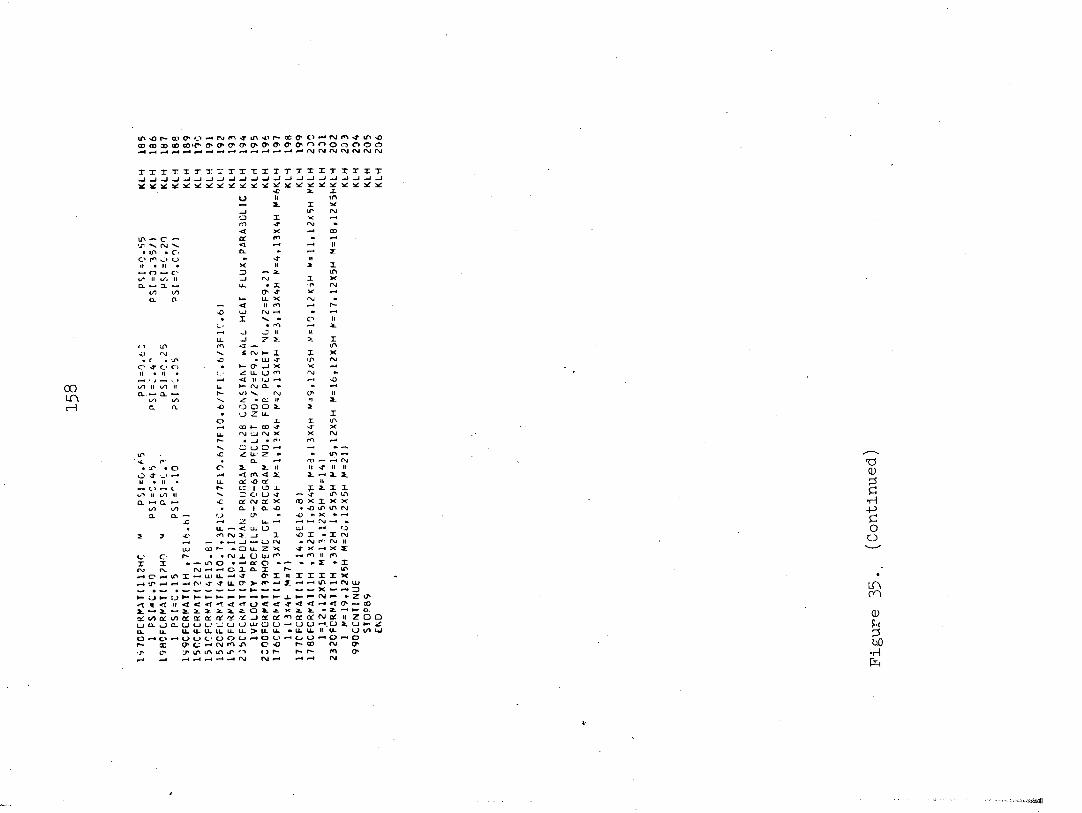
tO r- 00 O rg <- <1 C") m < o œ 00 CD •c* Ch O Ch (T O Ch a» Ch a» rt O O O o o o -1 -* —1 rg rvi rg

I X T X X T T T T T X X T X X X X X X X X u u U _J u -J _j «J * * * %: * ad * 3d * * * *: x: * * * x:

«c 2. X U II m a. X

lT O X m <-<ï X

m C oc m

!/*• fN X. < u

m c- z

o fo u «a-X M 2 X o 3 2. m

_J X X Ch X r\i

O fN X O u

O Z 2 5. l

m £ (N X X rg

o «j- cr II IL u

«1 >0 iZ) k-

a. r- 2: a. •o o O o a. 2 u Z IL X

i X -T X

LL fM «M

O «C 2?

CL o O 2. a_ II >r

o >r «1 m < 2. 2. 2. 2. OÉ sO Of C O 7- X X Ci u in LA

a «c CSC C\J a X X 1 o. >0 ~o m rg Lh 2! u LU O 7 m ï X sO X X rvj

_J o <NJ M O z X Z o C- r- ± U UJ m m n m

X X o CC o z X ru C 1 I —« O m X LL ti­ <r X X X X •x X

tr «y IL er > fC Z m <M UJ X 3 M" o H- J. (N Z V -1 n < u < «T *t < U < <r >r < < < O 2. 2. 2. 2. 2. 2. O a. 2. 2. 2. a: <•) a: a: 0É a QC * u ac oc or a: r\j oé II Z o o Î_I U w U (_J a w u o Z U z IL. u. u. IL LL > IL LL IL IL w O c» o O O O O o f- X (T C m C O CD CM Ch

o C ) P- m Ch rxj rg

T3 0) g •H -P C o O

LA on

0) b y bO

•H k

159

H O L M A N P R O G R A M N O . 2 9 C O N S T A N T W A L L T E M P E R A T U R E , P L U G F L O W K L H 0 0 1 S E P T E M B E R 2 3 , 1 9 6 3 . K L H 0 0 2 D I M E N S I O N A t 7 0 0 ) , B t T O O ) i A C ( 3 2 ) , X I 4 0 ) , Y ( 4 0 ) , V ( 4 0 ) , U ( 4 0 ) , T H E T A ( 4 0 , 2 1 K L H 0 0 3

1 ) t C ( 3 2 ) , A S Q ! 3 2 ) , E ( 3 2 ) , R I 2 1 ) , Z ( 4 0 ) , B 1 ( 3 2 ) K L H 0 0 4 C O M M O N A , B , A C , X , V , V , U , T H E T A , C , A S Q , E , R . Z . B l K L H 0 0 5

1 0 R E A D I N P U T T A P E 5 , 5 0 , M . M A N , N E L , P I E K L H 0 0 6 2 0 R E A D I N P U T T A P E 5 , 5 I t ( A d ) , 1 = 1 , M l K L H 0 0 7 3 0 R E A D I N P U T T A P E 5 . 5 1 , ( X ( I ) , 1 = 1 , N E L ) K L H 0 0 8

C A L L B E S S J I M , 1 , A , B 1 ) K L H 1 0 0 9 4 0 R ( 1 ) = 1 . 0 K L H 0 0 9 5 0 D 0 6 1 = 1 , 2 0 K L H 0 1 0 6 0 R ( ! • 1 ) " R ( I ) - . 0 5 K L H O i l 7 0 D O 8 1 = 1 , 2 0 K L H 0 1 2

N « M » I K L H 0 1 3 DO e J=1,M K L H 0 1 4 J A P = N * J K L H 1 0 1 4

8 0 A ( J A P ) = A f J ) » R ( I * 1 ) K L H 0 1 5 N = M * 2 1 K L H 0 1 6 C A L L B E S S J ( N , 0 , A , B ) K L H 0 1 7 0 0 9 1 = 1 , M K L H 0 1 8 A C ( I ) = B 1 € I ) / A ( I ) K L H 0 1 9 C ( I ) - 2 . / ( A ( I )»B l (m K L H 0 2 0

9 0 A S 0 C I > = 1 . / ( A ( I ) » A ( I ) ) K L H 0 2 1 1 0 0 R E A D I N P U T T A P E 5 . 5 2 . P K L H 0 2 2

I F ( P ) 1 , 9 9 , 1 1 K L H 0 2 3 1 1 0 W R I T E O U T P U T T A P E l O , 6 2 , * P K L H 0 2 4

0 0 1 2 1 = 1 , M K L H 0 2 5 1 2 0 E ( I ) * ( 1 . - S Q R T F ( 1 . « - 4 . » A t I ) « A ( I ) / ( P » P ) ) ) » P » P / 2 . K L H 0 2 6

D O 1 6 1 = 1 , N E L K L H 0 2 7 T = 0 . K L H 0 2 8 S U M - O . K L H 0 2 9 D O I S J = 1 , M K L H 0 3 0 A R G « X ( I ) » E ( J > K L H 0 3 1 I F ( A R G + 1 1 2 . ) 1 5 , 1 5 , 1 4 K L H 0 3 2

1 4 0 S N A P = E X P F ( A R G > K L H 0 3 3 T = T * S N A P K L H 0 3 4 S U M = S U M * S N A P / A S O ( J ) K L H 0 3 5

1 5 0 C 0 N T I N U E K L H 0 3 6 U l l ) = T / S U M K L H 0 3 7 V I I ) = U ( I ) / 5 . 7 5 K L H 0 3 8 Y ( I > = 4 . « S U M K L H 0 3 9 Z ( I > = P I E » ( 1 . - Y ( 1 ) ) / 4 . K L H 0 4 0

1 6 0 C 0 N T I N U E K L H 0 4 1 0 0 2 5 1 = 1 , N E L , K L H 0 4 2 0 0 2 5 J = 1 , 2 1 K L H 0 4 3 S U M = 0 . K L H 0 4 4 N=J«M - M K L H 0 4 5 0 0 2 4 K = 1 , M K L H 0 4 6 A R G = X ( I ) » E ( K ) K L H 0 4 7 I F ( A R G + 1 1 2 . > 2 4 , 2 4 , 2 3 K L H 0 4 8

2 3 0 J A P = N + K K L H 0 4 9 S U M = S U M » C ( K ) » B ( J A P ) » E X P F ( A R G ) K L H 1 0 4 9

2 4 0 C O N T I N U E K L H 0 5 0 2 5 0 T H E T A t I , J I - S U M K L H 0 5 1

W R I T E O U T P U T T A P E 1 0 . 5 3 , I I , A C ( I ) , C ( I ) , E ( I ) , I = 1,M> K L H 0 5 2 W R I T E O U T P U T T A P E I O . 5 4 , ( X ( I ) , U ( I > , V ( I ) , Y ( I ) , Z ( I ) , 1 = 1 , N E L ) K L H 0 5 3 W R I T E O U T P U T T A P E 1 0 , 6 3 , P K L H 0 5 4 W R I T E O U T P U T T A P E 1 0 , 5 5 K L H 0 5 5 0 0 2 6 1 = 1 , N E L K L H 0 5 6

2 6 0 W R I T E O U T P U T T A P E 1 0 , 5 6 , X ( I ) , ( T H E T A ( I , J ) , J = 1 5 6) K L H 0 5 7 W R I T E O U T P U T T A P E 1 0 , 5 7 K L H 0 5 8 0 0 2 7 1 = 1 , N E L K L H 0 5 9

Figure 36. Model III. Constant wall temperature - plug flow - calculations

160

2 7 0 W R I T E 0 U T P U T T A P E 1 0 , 5 6 , X ( I ) , I T H E T A I I , J ) , J * 7 , 1 2 ) K L H 0 6 0 M R I T E O U T P U T T A P E 1 0 1 5 8 K L H 0 6 1 0 0 2 8 1 = 1 , N E L K L H 0 6 2

2 8 0 H R I T E 0 U T P U T T A P E 1 0 . 5 6 . X I I ) , ( T H E T A ( I , J ) , J = 1 3 , 1 8 ) K L H 0 6 3 W R I T E O U T P U T T A P E 1 0 , 5 9 K L H 0 6 4 0 0 2 9 1 = 1 , N E L K L H 0 6 5

2 9 0 W R I T E O U T P U T T A P E 1 0 , 6 0 , X I I ) , 1 T H E T A 1 1 , J » , J = 1 9 , 2 1 ) K L H 0 6 6 W R I T E O U T P U T T A P E l 0 , 6 1 , P K L H 0 6 7 G O T O l O K L H 0 6 8

5 0 0 F 0 R M A T ( 3 1 2 , E 1 5 . 8 > K L H 0 6 9 5 1 0 F 0 R M A T 1 4 E 1 5 . 8 ) K L H 0 7 0 5 2 0 F 0 R M A T 1 F 1 Q . 2 ) K L H 0 7 1 5 3 D F O R M A T 1 5 8 H H E X P A N S I O N C O E F F . = A ( M ) C O M P L E T E C O E F F I C I E N T E I G E N V A L K L H 0 7 2

1 U E / 1 1 4 , 2 E 2 1 . 8 , E 1 6 . 8 > ) K L H 0 7 3 5 4 0 F 0 R M A T I 9 6 H Z E T A L O C A L N U S S E L T N O . N U . L O C . / ( N U . = 3 . 6 5 8 ) M I K L H 0 7 4

1 X E 0 — M E A N T H E T A Q Z { P E = K e O « ( T W - T O > ) R A T 1 0 / t E 1 6 . 8 , E 1 7 . 8 , 3 K 1 9 . 8 ) ) K L H 0 7 5 5 5 0 F O R M A T t l H 0 , 6 X 5 H Z E T A . 1 0 X 9 H P S I = 1 . 0 0 , 8 X 9 H P S I = 0 . 9 5 , 8 X 9 H P S I = 0 . 9 0 , 8 X K L H 0 7 6

1 9 H P S I = 0 . 8 5 , 8 X 9 H P S I = 0 . 8 0 , 8 X 9 H P S I = 0 . 7 5 ) K L H 0 7 7 5 6 0 F 0 R M A T t I H . 7 E 1 6 . 8 I K L H 0 7 8 5 7 0 F O R M A T ( 1 H 0 , 6 X 5 H Z E T A . 1 0 X 9 H P S I = 0 . 7 0 , 8 X 9 H P S I = 0 . 6 5 , 8 X 9 H P S I = 0 • 6 0 , 8 X K L H 0 7 9

1 9 H P S I = 0 . 5 5 , 8 X 9 H P S 1 = 0 . 5 0 , 8 X 9 H P S I = 0 . 4 5 ) K L H 0 8 0 5 8 0 F 0 R M A T I 1 H 0 . 6 X 5 H Z E T A . 1 0 X 9 H P S I = 0 . 4 0 , 8 X 9 H P S I = 0 . 3 5 , 8 X 9 H P S I = 0 . 3 0 , 8 X K L H 0 8 1

1 9 H P S I * 0 . 2 5 , 8 X 9 H P S I = 0 . 2 0 , 8 X 9 H P S I = 0 . 1 5 ) K L H 0 8 2 5 9 C F 0 R M A T Î 1 H 0 . 6 X 5 H Z E T A . 1 0 X 9 H P S I = 0 . 1 0 , 8 X 9 H P S I = 0 . 0 5 , 8 X 9 H P S I = 0 . 0 0 ) K L H 0 8 3 6 0 0 F 0 R M A T I I H . 4 E 1 6 . 8 I K L H 0 8 4 6 1 0 F O R M A T ( 1 H 0 , 1 0 X 8 0 H E N D O F P R O G R A M N O . 2 9 C O N S T A N T W A L L T E M P E R A T U R E , P K L H 0 8 5

1 L U G F L O W W I T H P E C = P E C L E T N 0 . / 2 = F 9 . 2 ) K L H 0 8 6 6 2 0 F O R M A T I 8 3 H 1 H 0 L M A N P R O G R A M N O . 2 9 C O N S T A N T W A L L T E M P E R A T U R E -P L U G F L O K L H 0 8 7

1 W W I T H P E C = P E C L E T N U M B E R / 2 = F 9 . 2 ) K L H 0 8 8 6 3 0 F O R M A T t 1 H 0 . 2 5 X 4 5 H T H E R M A L P R O F I L E S F O R P L U G F L O W P E C L E T N O • / 2 = F 9 • 2 K L H 0 8 9

1 ) K L H 0 9 0 9 9 0 C O N T I N U E K L H 0 9 1

S T O P 8 9 K L H 0 9 2 E N D K L H 0 9 3

Figure 36. (Continued)

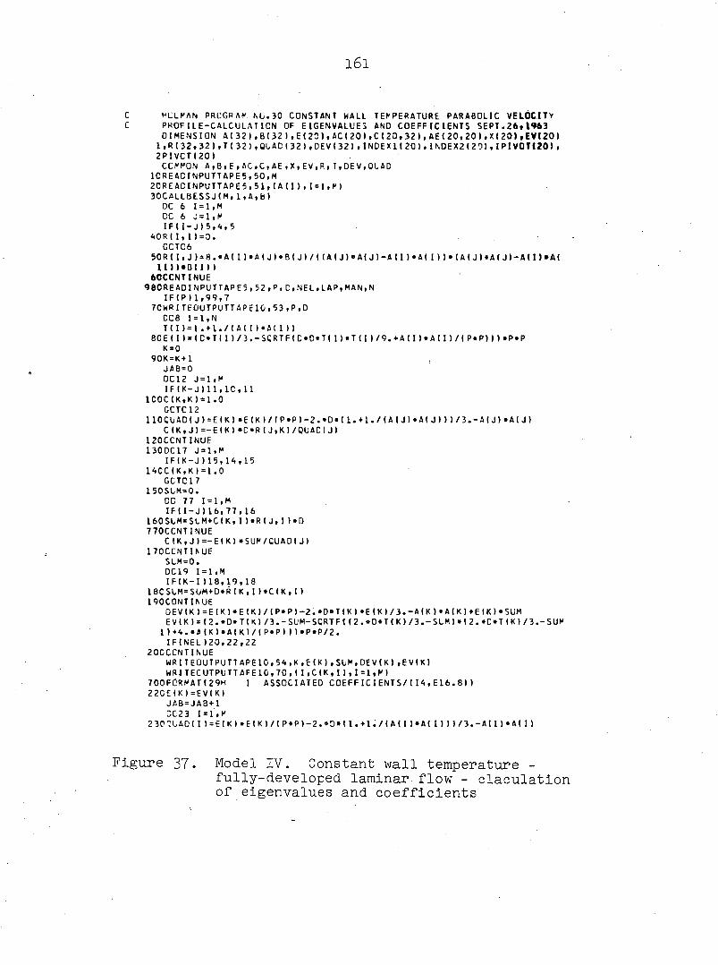
l6l

C H L L M A N P R C G P A N N U . 3 0 C O N S T A N T W A L L T E M P E R A T U R E P A R A B O L I C V E L O C I T Y C P R O F I L E - C A L C U L A T I O N O F E I G E N V A L U E S A N D C O E F F I C I E N T S S E P T . 2 6 , 1 9 6 3

D I M E N S I O N A ( 3 2 ) , B ( 3 2 ) , E ( 2 0 ) , A C < 2 0 ) , C t 2 0 , 3 2 ) , A E ( 2 0 , 2 0 ) , X ( 2 0 ) , E V C 2 0 ) 1 , R ( 3 2 , 3 2 ) , T ( 3 2 ) , 0 L A D ( 3 2 ) , D E V ( 3 2 ) , 1 N D E X 1 ( 2 0 ) , I N D E X 2 1 2 9 ) , I P I V 0 T 1 2 0 ) , 2 P I V C T I 2 0 )

C C N M O N A , B , E , A C , C , A E , X , E V , R , T , D E V , O V A C 1 0 R E A C I N P U T T A P E 5 , 5 0 , M 2 0 R E A C I N P U T T A P E 5 . 5 1 , ( A ( I ) , 1 = 1 , P ) 3 0 C A L L B E S S J ( M , 1 , A , B )

D C 6 1 = 1 , M C C 6 J = 1 , M I F ( : - J ) 5 , 4 , 5

4 0 R I I , I ) = 3 . G C T C 6

5 0 R ( I , J ) = 8 . « A ( I ) » A ( J ) * B ( J ) / ( ( A ( J ) » A ( J ) - A ( I ) « A ( I ) ) » ( A ( J ) » A ( J ) - A ( I ) » A ( 1 1 1 ) » 0 ( I ) )

6 0 C C N T I N U E 9 8 0 R E A D I N P U T T A P E 5 , 5 2 , P , D , N E L , L A P , M A N , N

I F ( P ) 1 , 9 9 , 7 7 C W R I T E 0 U T P U T T A P E 1 G , 5 3 , P , D

C C 8 1 = 1 , N T ( I ) = 1 . + ! . / ( A l I ) • A ( I ) )

8 0 E ( I ) = ( C » T ( I ) / 3 . - S C R T F ( C » D » T ( I ) » T ( I ) / 9 . + A ( I ) » A ( I ) / ( P » P ) ) ) » P » P K = 0

9 0 K = K * 1 J A B = 0 D C 1 2 J = 1 , M I F ( K - J ) 1 1 , I C , 1 1

1 C 0 C ( K , K ) = 1 . 0 G C T C 1 2

1 1 0 C U A D ( J ) = E ( K ) » E ( K ) / ( P * P ) - 2 . » D » ( l . + l . / ( A ( J ) * A ( J ) ) ) / 3 . - A ( J ) * A ( J ) C ( K , J ) = - E ( K ) » C » R ( J , K ) / Q U A C I J )

1 2 0 C C N T I N U E 1 3 0 D C 1 7 J = 1 , M

I F ( K - J ) 1 5 , 1 4 , 1 5 1 4 C C ( K , K ) = 1 . 0

G C T C 1 7 1 5 0 S L i M = 0 .

D C 7 7 1 = 1 , M I F ( I - J ) 1 6 , 7 7 , 1 6

1 6 0 S L M = S L M * C ( K , I ) » R I J , I ) » D 7 7 0 C C N T I N U E

C I K » J ) = - E ( K ) « S U K / C U A D I J ) 1 7 0 C C N T H U E

S L M = 0 . D C 1 9 1 = 1 , M I F I K - I ) 1 8 , 1 9 , 1 8

1 8 C S L M = S U M + D » R ( K , I ) * C ( K , I ) 1 9 0 C 0 N T I N U E

D E V ( K ) = E ( K ) » E ( K ) / ( P » P ) - 2 . » D ® T ( K ) » E ( K ) / 3 . - A ( K ) » A ( K ) + E ( K ) » S U M E V ( K ) = ( 2 . » D » T ( K ) / 3 . - S U M - S C R T F ( t 2 . • D » T { K ) / 3 . - S L M ) • ( 2 . « D * T ( K ) / 3 . - S U M

l ) + 4 . » M K ) * A ( K ) / ( P ' » P ) ) ) » P « P / 2 . I F I N E L ) 2 0 , 2 2 , 2 2

2 0 C C C N T I N U E W R I T E 0 U T P U T T A P E 1 C , 5 4 , K , E ( K ) , S U M , D E V ( K ) , E V ( K ) W R I T E C U T P U T T A P E I O , 7 0 , ( I , C I K , I ) , 1 = 1 , M

7 0 0 F C R M A T ( 2 9 H I A S S O C I A T E D C O E F F I C I E N T S / l 1 4 , E 1 6 . 8 ) ) 2 2 C E ( K ) = E V ( K )

J A B = J A B * 1 C C 2 3 1 = 1 , M

2 3 0 1 L . A D ( I ) = E ( K ) » E ( K ) / ( P » P ) - 2 . » D » ( 1 . • 1 . / ( A ( I ) * A ( I ) ) 1 / 3 . - A I I ) » A ( I )

Figure 37. Model IV. Constant wall temperature -fully-developed laminar flow - claculation of eigenvalues and coefficients

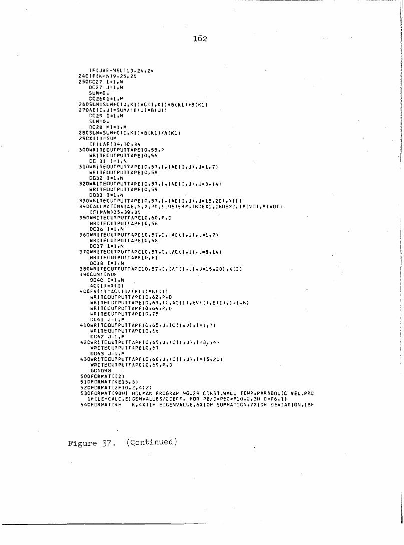
162

l F t J A E - N E L ) 1 3 , 2 4 , 2 4 2 4 C I F ( K - M 9 , 2 5 , 2 5 2 5 0 C C 2 7 1 = 1 , N

0 C 2 7 J 5 1 , N S U M = 0 . C C 2 6 K 1 = 1 , M

2 6 0 S L M = S L M + C ( J , K 1 ) » C I I , K l ) « B ( K l ) * 8 ( K l ) 2 7 0 A E ( I , J ) = S U M / ( B U ) o B ( J ) )

C C 2 9 1 = 1 , N SlM=0. D C 2 8 K l = l , M

2 8 C S L M = S L M + C ( I , K 1 ) • B ( K 1 ) / A ( K 1 1 2 9 0 X 1 1 ) = S U M

I F t L A F 1 3 4 , 3 0 , 3 4 3 0 0 W R I T E C U T P U T T A P E 1 0 , 5 5 , P

W R I T E C U T P U T T A P E 1 0 . 5 6 C C 3 1 1 = 1 , N

3 I 0 W R I T E O U T P U T T A P E 1 0 , 5 7 , I , ( A E I I , J ) , J = 1 , 7 ) W R I T E t J U T P U T T A P E l O , 5 8 C C 3 2 1 = 1 , N

3 2 0 W R I T E C U T P U T T A P E 1 0 , 5 7 , 1 , ( A E ( 1 , J ) , J = 8 , 1 4 ) W R I T E U U T P U T T A P E 1 C . 5 9 D C 3 3 1 = 1 , N

3 3 0 W R I T E C U T P U T T A P E 1 0 , 5 7 , 1 , ( A E ( I , J I , J = 1 5 , 2 0 > , X ( I ) 3 4 0 C A L L M # T I N V ( A E , N , X , 2 0 , 1 = D E T E R P , I N C E X 1 , U D E X 2 , I P I V O T . P I V O T )

I F I M A M 3 5 . 3 9 . 3 5 3 5 0 W R I T E C U T P U T T A P E 1 0 , 6 0 , P , 0

W R I T E C U T P U T T A P E I O , 5 6 D C 3 6 1 = 1 , N

3 6 0 W R I T E O U T P U T T A P E 1 0 , 5 7 , 1 , I A E ( I , J ) , J = 1 , 7 ) W R I T E C U T P U T T A P E I O , 5 8 0 0 3 7 1 = 1 , N

3 7 0 W R I T E O U T P U T T A P E 1 G , 5 7 , 1 , ( A E < I , J ) , J = 8 , 1 4 ) W R I T E C U T P U T T A P E I O , 6 1 D C 3 8 1 = 1 , N

3 8 0 W R I T E C U T P U T T A P E I O , 5 7 , 1 , ( A E ( I , J ) , J = 1 5 , 2 0 ) , X { I ) 3 9 C C 0 N T I N U E

0 0 4 C 1 = 1 , N A C C I ) = X ( I )

4 0 Q E V ( I l = A C ( 1 1 / ( B ( I ) « B ( H ) W R I T E O U T P U T T A P E 1 0 , 6 2 , P , D W R I T E C U T P U T T A P E 1 0 , 6 3 , ( I , A C ( I I , E V ( I ) , E ( I ) , I = 1 , M W R I T E C U T P U T T A P E 1 0 , 6 4 , P , D W R I T E C U T P U T T A P E I O , 7 5 C C 4 1 J = 1 , M

4 1 O W R I T E O U T P U T T A P E 1 0 , 6 5 , J , I C I I , J ) , I = 1 , 7 ) W R I T E O U T P U T T A P E 1 0 , 6 6 C C 4 2 J = l , M

4 2 0 W R I T E O U T P U T T A P E 1 0 , 6 5 , J , ( C ( I , J ) , I = 8 , 1 4 ) W R I T E C U T P U T T A P E I O , 6 7 0 0 4 3 J = 1 , M

4 3 0 W R I T E O U T P U T T A P E 1 0 , 6 8 , J , I C I I , J ) , I = 1 5 , 2 0 ) W R I T E O U T P U T T A P E 1 0 , 6 9 , P , D G C T 0 S 8

5 0 0 F C R K A T I I 2 ) 5 1 0 F 0 R M A T 1 4 E 1 5 . 8 ) 5 2 C F C R M A T ( 2 F 1 0 . 2 , 4 I 2 ) 5 3 0 F C R M A T I 9 8 H 1 H C L M A N P R O G R A M N C . 2 9 C O N S T . W A L L T E M P , P A R A B O L I C V E L

I F I L E - C A L C . E I G E N V A L U E S / C O E F F . F O R P E / D = P E C = F 1 0 . 2 , 3 H 0 = F 6 . 1 ) 5 4 C F 0 R M A T I 4 H K . 4 X 1 1 H E I G E N V A L U E , 6 X 1 0 H S U M M A T I O N , 7 X 1 0 H D E V I A T I O N

Figure 37. (Continued)

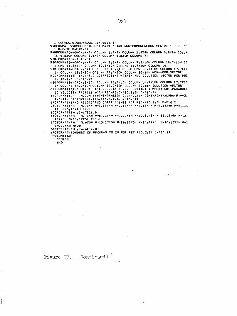
163

1 R E C A U C . E I G E N V A L U E / , 1 4 , 4 6 1 6 . 8 ) 5 5 0 F O R M A T ( 5 5 H O C O E F F I C I E N T M A T R I X A N D N O N - H O M O G E N E O U S V E C T O R F O R P E C = F

1 1 0 . 2 , 3 H 0 = F 1 0 . 2 ) 5 6 0 F 0 R M A T ( 4 H 0 R C W . 4 X 9 H C O L U M N 1 , 8 X 9 H C O L U M N 2 . 8 X 9 H C O L U M N 3 . 8 X 9 H C O L U f

I N 4 , 8 X 9 H C O L U M N 5 . 8 X 9 H C O L U M N 6 . 8 X 9 H C O L U M N 7 ) 5 7 0 F C R M A T ( I 4 , 7 E 1 6 . 6 ) 5 8 C F C R M A T I 4 H 0 R 0 H . 4 X 9 H C O L U M N 8 , 8 X 9 H C O L U M N 9 . 8 X 1 C H C O L U M N 1 0 . 7 X I O H C C

1 L L M N U . 7 X 1 0 H C C L L M N 1 2 . 7 X 1 0 H C O L U M N 1 3 . 7 X 1 0 H C C L U M N 1 4 ) 5 9 0 F O R M A T I 4 H O R O W . 3 X 1 C H C O L U M N 1 5 , 7 X 1 O H C C L U M N 1 6 . 7 X 1 C H C O L U M N 1 7 , 7 X 1 0

I H C O L U M N 1 8 , 7 X 1 C H C O L U M N 1 9 , 7 X 1 C H C C L U M N 2 0 , 1 6 H N O N - H O M O . V E C T O R I 6 0 0 F C R M A T I 5 7 H I N V E R T E D C O E F F I C I E N T M A T R I X A N D S O L U T I O N V E C T O R F O R P E C

1 = F 1 0 . 2 , 3 H D - F 1 0 . 2 ) 6 1 0 F C R M A T ( 4 H 0 R 0 W . 3 X 1 C H C O L U M N 1 5 . 7 X 1 0 H C O L U M N 1 6 . 7 X 1 C H C O L U M N 1 7 , 7 X 1 0

I H C O L U M N 1 8 . 7 X 1 C H C O L U M N 1 9 , 7 X 1 0 H C C L U M N 2 0 , 1 6 H S O L U T I O N V E C T O R ) 6 2 0 F 0 R M A Î I 8 9 H 0 0 U T P U T D A T A P R O G R A M N O . 2 9 C O N S T A N T T E M P E R A T U R E , P A R A B O L l

I C V E L O C I T Y P R O F I L E W I T H P E C = P E / 0 = F I C . 2 , 3 H C = F 1 0 . 2 ) 6 3 0 F C R M A T ( 4 H M , 2 2 H A ( M ) = E X P A N S I O N C O E F F . , 2 3 H D ( M I = A ( M ) / A L P H A ( M ) » « 2 .

1 , 6 X 1 1 1 - E I G E N V A L U E / I I 4 . E 1 6 . 8 , E 2 8 . 8 . E 1 6 . 8 ) ) 6 4 C F C R M A T ( 3 4 H 0 A S S O C I A T E D C O E F F I C I E N T S F O R P E C = F 1 0 . 2 , 3 H 0 = F 1 0 . 2 ) 7 5 0 F C R M A T ( 4 H N . 7 X 4 H M = l , 1 3 X 4 H M = 2 , 1 3 X 4 H M = 3 , 1 3 X 4 1 - M = 4 , 1 3 X 4 H M = 5 , 1 3 X

1 4 h M = 6 , 1 3 X 4 H M = 7 ) 6 5 0 F C R M A T ( I H , I 4 , 7 E 1 6 . 8 ) 6 6 0 F O R M A T ( 4 H N . 7 X 4 H M = 8 , 1 3 X 4 H M = 9 , 1 2 X 5 H M = 1 0 , 1 2 X 5 H M = 1 1 , 1 2 X 5 H M = 1 2 ,

1 1 2 X 5 H M = 1 3 , 1 2 X 5 h M » 1 4 ) 6 7 0 F 0 R M A T ( 4 H N . 6 X 5 H M = 1 5 , 1 2 X 5 H M = 1 6 , 1 2 X 5 H M = 1 7 , 1 2 X 5 H M = 1 8 , 1 2 X 5 H M « 1

1 9 . 1 2 X 5 H M = 2 0 ) 6 8 0 F O R M A T ( I H , I 4 . 6 E 1 6 . 8 ) 6 9 0 F C R M A T ( 3 0 H 0 E N C C F P R O G R A M N O . 2 9 F O R P E C = F I 0 . 2 , 3 H D = F I C . 2 ) 9 9 C C 0 N T I h U E

S T 0 P 8 9 E N D

Figure 37. (Continued)

164

C P 3 4 0 0 1 C H C L M A N P R O G R A M N O . 3 4 C A L C U L A T I O N O F C O E F F I C I E N T S U S I N G I N P U T E I G E N P 3 4 0 0 2 C - V A L U E S A N D / O R A S S O C I A T E D C O E F F I C I E N T S N O V E M B E R 4 , 1 9 6 3 P 3 4 C 0 3 C P 3 4 0 0 4

D I M E N S I O N A ( 3 2 ) , B ( 3 2 ) , R ( 3 2 , 3 2 > , C ( 3 2 , 3 2 > , S S A V E ( 3 1 , 3 1 ) , I N O E X l ( 3 1 ) , I N P 3 4 0 0 5 1 D E X 2 1 3 1 ) , P I V 0 T ( 3 1 ) , I P I V O T ( 3 1 ) , D ( 3 1 ) , P ( 3 2 ) , S ( 3 1 , 3 1 ) , X ( 3 2 ) , A E ( 3 1 , 3 1 ) P 3 4 0 0 6 2 , C O E ( 3 2 , 3 2 l , V ( 3 1 ) P 3 4 0 0 7

C C M M C N A , B , ' P , C , S S A V E , C , P , S , X , A E , C O E , V , I N D E X 1 , I N D E X 2 . P I V C T . I P I V O T P 3 4 0 0 8 1 C R E A D 5 0 , N , N E L , M I T P 3 4 0 0 9

G C T O ( 8 0 , 3 9 ) , M I T P 3 4 0 1 0 5 1 0 F C R M A T 1 4 E 1 5 . 8 ) P 3 4 0 1 1 5 0 0 F C R M A T ( 3 1 2 ) P 3 4 0 1 2 8 0 0 R E A D 5 1 , ( A ( I ) , 1 = 1 , N ) P 3 4 0 1 4

C A L L B E S S J ( N , 1 , A , Ë ) P 3 4 0 1 5 G C T O ( 2 , 3 9 ) , N E L P 3 4 0 1 6

2 G C C 5 1 - 1 , N P 3 4 0 1 7 A I S » A ( I ) » A l I ) P 3 4 0 1 8 S L M = 1 6 . 0 e A ( I ) / B ( I ) P 3 4 0 1 9 P ( I ) = 4 . » ( 1 . + 1 . / A I S J / 3 . P 3 4 0 2 0 R ( I , I > = A I S P 3 4 0 2 1 D C 5 J = 1 , N P 3 4 0 2 2 I F ( I - J ) 3 , 5 , 3 P 3 4 0 2 3

3 0 A J S = A ( J ) « A ( J ) P 3 4 0 2 4 A J M I = # J S - A I S P 3 4 0 2 5

4 0 R ( I , J ) = S U M » A ( J ) * B ( J ) / ( A J M I » A J M I ) P 3 4 0 2 6 5 0 C C N T I N U E P 3 4 0 2 7

C P 3 4 0 2 8 C C O M P U T E N O N - H O M O G E N E O U S S Y S T E M U S I N G I N P U T E I G E N V A L U E P 3 4 0 2 9 C P 3 4 0 3 0

6 0 R E A C 5 2 , P E C P 3 4 0 3 1 5 2 0 F C R M A T I F 1 0 . 2 ) P 3 4 0 3 2

I F ( P E C ) 1 , 9 9 , 7 P 3 4 0 3 3 7 0 P R I N T 5 3 , P E C P 3 4 0 3 4

5 3 0 F 0 R M A T ( 1 H 1 5 X 8 2 H H O L M A N P R O G R A M N O . 3 4 C A L C U L A T I O N O F A S S O C I A T E D C 0 P 3 4 0 3 5 1 E F F 1 C I E N T S F O R P E C L E T N U M B E R / 2 = F 1 0 . 2 > P 3 4 0 3 6

9 4 C F C R M A T I I 2 , E 1 5 . 8 , 3 1 2 ) P 3 4 0 3 7 8 C R E A D 9 4 , M , E , N O P T , K A T , K O P T P 3 4 1 0 3 7

I F ( M ) 6 , 6 , 9 P 3 4 0 3 8 9 C C C 1 1 1 = 1 , N P 3 4 0 3 9

C ( I , l ) = E » E / ( P E C « P E C ) - P ( I ) » E - R ( l , I ) P 3 4 0 4 0 D O 1 1 J = 1 , N P 3 4 0 4 1 I F ( I - J 1 1 0 , 1 1 , 1 0 P 3 4 0 4 2

1 0 C C ( I , J ) * E * R ( I , J ) P 3 4 0 4 3 1 1 C C C N T I N U E P 3 4 0 4 4

M A P = N - 1 P 3 4 0 4 5 C C 1 2 1 = 1 , M A P P 3 4 0 4 6

1 2 C C I I ) = - C ( I , M ) P 3 4 0 4 7 L = M + I P 3 4 1 0 4 7 J A P = M - 1 , P 3 4 0 4 8 I F ( J A P ) 1 5 , 1 3 , 1 5 P 3 4 C 4 9

1 3 0 C C 1 4 1 = 1 , M A P P 3 4 0 5 0 C O 1 4 J = 2 , N P 3 4 0 5 1

1 4 0 5 ( 1 , J - 1 ) = C ( I , J ) P 3 4 0 5 2 G O T O 2 2 P 3 4 0 5 3

1 5 0 I F t J A P - 1 ) 1 9 , 1 6 , 1 9 P 3 4 0 5 4 1 6 0 C C 1 7 1 = 1 , M A P p 3 4 0 5 5 1 7 0 S ( 1 , 1 ) = C ( I « 1 ) P 3 4 0 5 6

D C 1 8 1 = 1 , M A P P 3 4 0 5 7 D C 1 8 J = 3 , N P 3 4 0 5 8

Figure 38. Model IV. Constant wall temperature - fully-developed laminar flow - calculation of coefficients with input eigenvalues

059 060 C61 062 063 064 065 066 067 068 069 070 071 072 073 074 075 076 077 078 079 080 0 8 1 C82 C83 084 085 086 087 088 089 090 091 092 093 094 095 096 097 098 099 100 101 102 103 104 105 106 107 1 0 8 109 110 111 1 1 2 113 114 115 1 1 6 117 116 119 12C

165

1 8 C S ( I , J - 1)=C( I,J> G C T O 2 2 ? \ l

1 9 0 0 C 2 0 1 = 1 , M A P p

C L 2 0 J = 1 , J A P p f ;

2 0 C S t I , J ) = C ( I , J ) pi , C C 2 1 1 = 1 , M A P p H

D C 2 1 J = L , N p : :

2 1 0 S ( I , J - 1 ) = C ( I , J ) p^; 2 2 0 C C N T I N U E * ,

G C T O ( 2 3 , 2 5 ) , N O P T p , ?

2 3 0 D C 2 4 1 = 1 , M A P ' I

D C 2 4 J = 1 , M A P ' .

2 4 0 S S A V E I I , J ) = S ( I , J ) p 3 1

2 5 0 C A L L M A T I N V(S,MAP,C,31,l.DETERM,IiNCEXl,INDEX2,IPIV C T,PIV O T ) P34 I F ( J A P ) ? 6 , ? f c , 2 8 p g ,

2 6 c x ( n = i .0 p I: DC 27 1=1,MAP p

270X(I•1)=D( I ) GC TO 31 p%

280DC 29 1=1,JAP f p:7 29CX(I)=C(I) p,7

x ( M ) = 1 . 0 p : %

CC 30 I = M, MAP p" 3 OOX C1*11=0(1) ' . 3 i o s u m = O . : iz

C C 3 2 1 = 1 , N > p L

3 2 C S U M = S U M + C ( N , I ) » X ( I ) p 3 < |

P R I N T 5 4 , M , E , D E T f c R M , N , S U M p 3 4

5 4 0 F C R M A T ( 5 5 H 0 M E I G E N V A L U E D E T E R M I N A N T N E C U A T I 0 N - C H E C K / P 3 4 M 1 H 0 , 1 4 , 2 E 1 7 . f i , 1 3 , £ 1 7 . 0 ) ) p 3 4

P R I N T 5 5 p 3 4

5 5 0 F C R M A T ( 3 1 H O A S S O C I A T E O C O E F F I C I E N T S , 8 Y R O W ) P 3 4 P R I N T 5 6 , ( X I I > , I = 1 , N ) p , .

5 6 0 F C R M A T ( l H O / t 7 E 1 7 . f i ) ) p 3 4

G C T U ( 3 3 , 3 6 ) , N O P T p 3 4

3 3 C P R I N T 5 7 p 3 4

5 7 0 F C R M A T ( 1 H J 3 X 4 6 H E L E M E N T S C F O R I G I N A L A U G M E N T E D M A T R I X , B Y R O W S ) P 3 4 D C 3 4 1 = 1 , M A P P 3 4

3 4 C P R I N T 5 6 , ( S S A V E ( I , J ) , J = 1 , M A P I , C ( I , M ) p 3 4

P R I N T 5 8 p 3 4

5 8 0 F C R M A T ( 1 H J 3 X 2 8 H E L E M E N T S O F I N V E R S E , B Y P . O W S ) P 3 4 D C 3 5 1 = 1 , M A P p 3 4

3 5 C P R I N T 5 6 , ( S ( I , J ) , J = 1 , M A P ) p 3 4

3 6 C C C 3 7 1 = 1 , N P 3 4

3 7 0 C C 1 E ( M , I ) = x ( I ) p 3 4

G C T O ( 3 8 , 8 ) , K A T ' P 3 4

3 8 C G C T O ( 4 1 , 3 9 ) , K C P T p 3 4

3 9 C R E A D 6 0 , L I , N I P . , K O P T , P E C p 3 < t

D C 4 D 1 = 1 , L I P 3 4 4 0 0 R E A D 5 1 , ( C O E ( I , J ) , J = 1 , N I P ) P 3 4

G C T O 4 2 p 3 4

4 1 C R E A D 6 0 , L I , N I P , K O P T , P E C p a t ,

4 2 0 P R 1 N T 6 1 , P E C P 3 4

P 3 4 C C A L C U L A T E E X P A N S I C N C O E F F I C I E N T S p 3 4

C P 3 4 DC 4 5 I = 1 » L I P 3 4 SL M=0• P34 CC 43 J=l,NIP p34

4 3CSLM=SLM+CQE( I , J ) »E(J)/A(J) p34 D{I)=— SUM P3 4 V ( I Î = SUw P3A

Figure 38; (Continued)

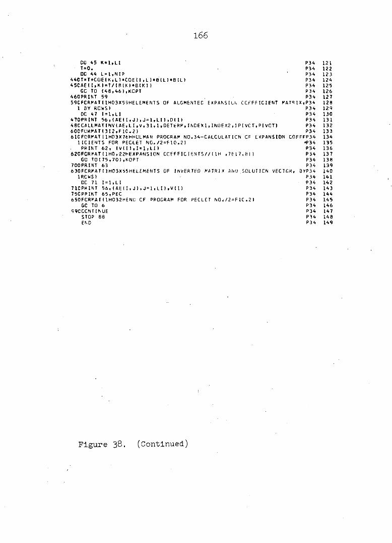
166

DC 45 K=l,Ll P34 T*0. P34 CC 44 L = 1 » N I P P34

44C T*T+CGE(K, L )• C0EII,L)*8(L)<»B(L) P34 45CAEII,K)=T/IB(K)»e(K)) P34

GC TO (48,46),KCPT P34 460PRINT 59 P34 59CFCRMAT(1H03X59HELEME NT S OF AUGMENTED EXPANSION COEFFICIENT MATRIX,P34

1 BY ROWS) P34 DC 4 7 1=1,LI P34

4 70PRINT 56, (AE(I,J),J=1,LI),0(I) P34 4 8CCALLMATINV(AE,LI,V,31,1,DE TERM,INDEX 1,INDEX2,1PIVCT.PIVCT) P34 600FURMAT(3I2,F1C.2) P34 6ICFORMATt 1 HO 3X 7é H80L MA N PROGRAM NO.34-CALCULATICN CF EXPANSION C0FFFP34

1ICIENTS FOR PECLET N0./2=F10.2) «P3 4 PRINT 62, (Vll1,1=1,LI) P34

62CFGRMAT ( 1 HO , -22t*EXPANS I ON COEFFICIENTS//! IH ,7617.8) ) P34 GC TO( 75,70) ,KOPT P34

700PR I NT 63 P34 6 30FCRMATI 1 HO3X55HELEMENTS OF INVERTED MATRIX AM) SOLUTION VECTGH, 0YP34

I ROWS) P34 DC 71 1 = 1,LI P34

71CPKINT 56, (AEII,J),J=1,LI),V(I) P34 75CPRINT 65,PEC P34 650FORMAT(1H0 32HEND CF PROGRAM FOR PECLET N0é/2=FIC.2) P34

GC TO 6 P34 99CCCNTINUE P34

STOP 88 P34 END P34

1 2 1 1 2 2 123 124 125 126 127 1 2 8 129 130 131 132 133 134 135 136 137 13 H 139 140 141 142 143 144 145 146 147 148 149

Figure 38. (Continued)

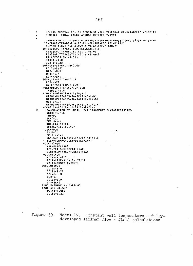
167

C HOLMAN PROGRAM NO. 31 CONSTANT WALL TEMPERATURE-PARABOLIC VELOCITY C PROFILE -FINAL CALCULATIONS OCTOBER 7,1963 C

DIMENSION AI700),B(7CO),C(20,32>>E(20)iT(40,21),RADI?3),X(40),Y(40 11,Z140),YZ(40),CHA(20,21I , AC ( 201.COE1201,B1(32) COMMON A,B,C,T,CHA,X,Y,Z,YZ,AC,C0E,E,RA0,B1

1CREADINPUTTAPE5,7&,M,NEL.KATE .PIE REACINPUTTAPE5.76,(All),1=1,M) READINPUTTAPE5.76,I X I I),I = 1,NEL) CALLBESSJ(M,1,A,B1) RAOI11=1.0 002 1=1,20

20RADIItl)=RAD( I 1-0.05 CC 3J*2,21 NAB=J»M-M DC3I=1,M L I P=NAB+I

30A ! LIP)=AI I )»RADIJ) L1P=M»21 CALLBESSJ(LIP,0,A,Bl

4CREA01NPUTTAPE5,77,P.D.N IFIP)1,99,5

50WRITEOUTPUTTAPE 10,78,P,D READINPUTTAPE5,76,(El I),I = 1,N) READINPUTTAPE5,76,I AC I I),1 = 1,M 0C6 1=1,N READ IN PUTTAPE 5,76,(C(I , J) , J=1,M>

60CCEI I) = ACm«2./(Bl(l)»Bim ) C CALCULATION OF LOCAL HEAT TRANSPORT CHARACTERISTICS

CC10 I = 1,NEL T0T=0. SLMT=0. 009 J=1,N ARG-EIJ)»XII ) IFIARG-f-112.19,9,7

7CSLM=0.0 . TSUM=0. CC 8 K=1,M SUM=SLM*C(JiK)»Bl(K)/(A(K>»»3.) TSUM=TSUM+C(J,K)*Bl(K)*A(K)

80CCNTINUE YAP=EXPF(ARC) TCT=TOT+SUM«CCE(J)»YAP SLMT = SUM T + TSUM*COE(J)•YAP

90CCNTINUE Y 111 = 16.»TOT Z I I ) = IPIE/4.)•11.-Y I I)) YZII)=SUMT/I8.»T0T)

1COCCNTINUE 0C12K=1,N DC12J=1 » 21 MEL=M»J-M SLM=0. CC11I=1,M LA=MEL*I

110SUM=SUMtC(K,I)*EILA) 120Ct-AIK,J) = SUM

CC151=1,NEL 0C15J=1,21

Figure 39. Model IV. Constant wall temperature - fully-developed laminar flow - final calculations

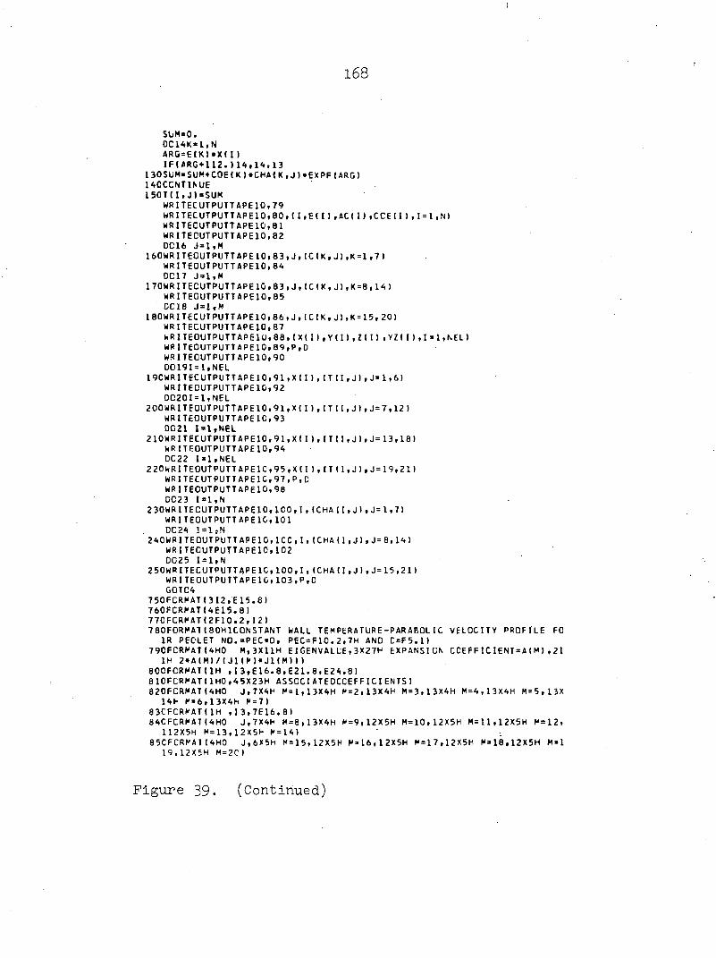
I

168

SUM=0. OC14K*1,N ARG=E(K)«XI I ) IFIARGH12.)14,14,13

130SUM-SUM+C0EIK)»CHA(K,J)»EXPF(ARG) 14CCCNTISUE 150T(I,J)= SUM

WRITECUTPUTTAPEIO,79 WRITECUTPUTTAPE10.80,tI,E(I),AC( I > ,CCE( I ) , 1 = 1 ,N) WRITECUTPUTTAPEIO,81 WRITECUTPUTTAPEIO,82 DC16 J=1,M

160WRITE0UTPUTTAPE10,83,J,(C(K,J),K=1,7) WRITECUTPUTTAPEIO,84 DC17 J=1,M

170WRITECUTPUTTAPE1G,83,J,(CIK,J),K=8,14) WRITECUTPUTTAPEIO,85 DC 18 J = 1,M

180WRITECUTPUTTAPE10.86,J,(CIK,J),K=15, 20) WRITECUTPUTTAPEIO,87 WRITECUTPUTTAPEIO,88,(XI I),Y II),Z II ) ,YZII),1 = 1,NEL) WRITE0UTPUTTAPE10,89,P,D WRITECUTPUTTAPEIO,90 00191=1,NEL

19CWRITECUTPUTTAPE10.91,XII),IT11,J) , J=1,6) WRITECUTPUTTAPEIO,92 00201=1,NEL

200WRITEOUTPUTTAPE 10,91,XI I ) , I T11,J1,J=7,12) WRITE0UTPUTTAPE1C.93 0021 1 = 1,NEL

210WRITECUTPUTTAPE10.91.XII),(TII,J),J=13,18) WRITEOUTPUTTAPE10.94 0C22 1=1,NEL

220WRITE0UTPUTTAPE10,95,XII),(T I 1,J),J=19,21) WRITECUTPUTTAPE1G,97,P,D WRITECUTPUTTAPEIO,98 CC23 1 = 1,N

2 30WRITECUTPUTTAPE10.1C0,1,ICHA 11,J),J=1,7) WRITECUTPUTTAPEIO,101 DC 24 1=1,N

240WRITECUTPUTTAPE10,ICC,I,ICHA11,J),J=8,14) WRITECUTPUTTAPEIO,102 0025 1=1,N

2 50WRITECUTPUTTAPE1C.100.I,ICHA II,J),J=15,21) WRITE0UTPUTTAPE1G,10 3,P,0 GCTC4

750FCRMAT1312,E15.8) 760FCRMATI4E15.8) 770FCRMATI2F10.2, 12) 780FORMAT18OH ICON ST ANT WALL TEMPERATURE-PARABOLIC VELOCITY PROFILE FO

1R PECLET NO.=PEC»D, PEC=F10.2,7H AND C=F5.1) 7 9C FCRMAT 14H0 M.3X11H EIGENVALUE,3X27H EXPANSION COEFF ICIENT = AIM),21

IH 2»A(M)/IJ1IM)»J11M))) 800FCRMATIIH ,I 3,E16.8,E21.8,E24.8) 810FCRMAT II HO,45X23H ASSOC IATEDCCEFF ICIENTS) 820FCRMATI4H0 J.7X4H M=l,13X4H M=2,13X4H M=3,13X4H M=4,13X4H M=5,13X

141- M = 6,13X4h M = 7 ) 83CFCRMATIIH ,I3,7E16.8) 84CFCRMATI4H0 J,7X4h M = 8,13X4H M = 9,12X5H M=10, 12X5H M=11,12X5H M=12,

112X5H M=13,12X5H M=14) 85CFCRMAII4H0 J.6X5H M=15,12X5H M=16,12X5H M=17,12X5H M=18,12X5H M = 1

19,12X5H M = 2C)

Figure 39. (Continued)

169

8 60FCRMAT(IH » I 3> 6E lfc.8) 87CFCRMAT(1H1,6X5H ZLTA.6X17H MIXED-MEAN THETA, 1SH C/(PE»K»C*<TN-TI ))

1.21H LOCAL NUSS6LT NUMBER) 880FCRMAT(IH ,2E16.8,E17.8,EIS.8) 890FCRMATI1H1.96H THERMAL PROFILES FOR CONSTANT WALL TEMPERATURE A

INC PARABOLIC VELOCITY PROFILE ta I TP Ft/D = PEC =F 10.2,7H AND C-F5.1) 90OFORMATI1H0.6X5H ZtTA,10X9H PS1=I.CC,8X9H PSI=C.95,8X9H PSI-0.9C.8X

19h PS1=0.85,8X9H PSI=0.60,8X9h PSI=0.75) 91CFCRMATI1H ,7E16.8) 92CFCRMAK 1H0.6X5H ZETA,10X9h P S I =C . 70, RX9H PSI =C.65,8X9I- PSI-0.60.8X

19h PSI=0.55,BX9H PSI=C.50,8X9H PSI=0.45) 930FCRMAT!1H0.6X5H ZLTA,10X91- PSI=C.40,8X9H PS I=0.35,8X9H PSI-0.30,8X

19h PS I=0.25,8X9H PSI=0.20,8XSh PSt=C.15) 94CFCRMATI1H0.6X5H ZETA.10X9H PS I =0.10,8X9H PS I=C.05,8X9H PSI«0.C0) 9 50FCRMATI1H .4E16.8) 970FCRMATI1H1,92t- CHARACTERISTIC FUNCTIONS FOR CONSTANT WALL TEMPERAT

1URE AND PARABCLIC VELOCITY PROFILE- PEC=F10.2,7H AND C=F5. 1 ) 98CFCRMAT(4HC, M,4X9H PSI=1.CC,8X9H PSJ=C.95,6X9h PS I=0.9C,8X9H PSI=0

1.85,BX9H PSI=C.8C,8X9H PSI=0.75,6X9h PSI=C.70) lOOOFORMAT(IH ,I3,7E 16.8) 1010FURMATI4H0 M,4X9H PSI=0.65,8X9H PSI=C.60,8X9H PSI=0.55,8X9H PSI=0

1.50.8X9H PSI =C .45, 8X9t- PSI =C .40, 8X9H PSI=0.35) 1C2CFCRMAT(4H0 M.4X9H PSI=C.3C,8X9H PSI=C.2 5,8X9H PSI=C.20,8X9H PSI=C

1.15,8X9H PSI=C.1C.8X9H PSI=C.C5,8X9H PS1=0.00) 1030FURMAT(61HLENH CF CALCULATIONS-CONSTANT T-POISEVILLE FLOW FOR PEC

1PE/C = F10.2,7H AND D= F5.1) 99CCCNTI NUE

IF(KATE) 125, 125,30 30CWRITECUTPUTTAPE10,1C4

WRITtCUTPUTTAPElC,lC5,(I,A(l),BI.I),I = l,LIP) WRITECUTPUTT APE1L,106 WRITECUTPUTTAPE11,107,tI,A(I ) ,B1 (I) ,I = 1,M)

1040FCRMAT(lHl,36h I X = ARGLNEN T J-ZtRO(X)/) 1C5CFCRMAT { IH ,14,21:18.8) 1C60F0RMATI1H1.33H I X=ROOT OF JC(X) J-ONE(X)/) 1C70FCRMAT( IH ,I 4,2E 16.8) 125CCCNTINUE

ST0P89 L \ 0

Figure 39. (Continued)

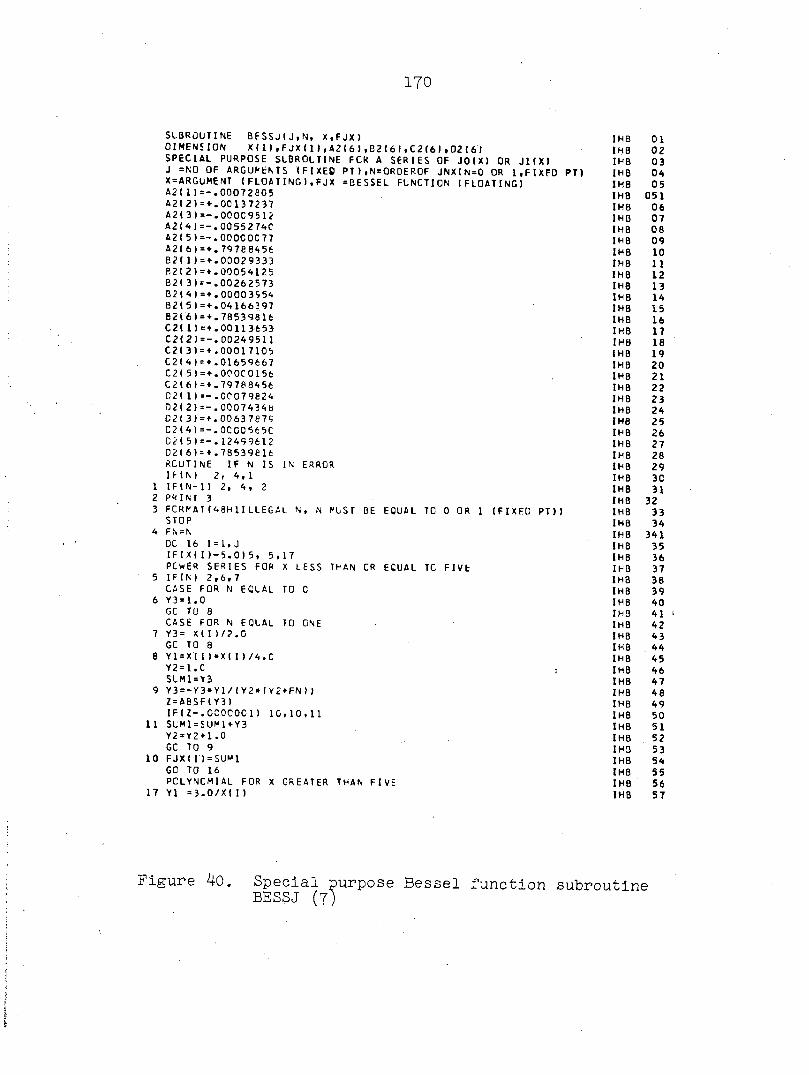
170

SUBROUTINE BESSJIJ,N, X,FJX) 01 MENS ION X(l|,FJX(l),A2(6l,B2(6l,C2(6l,02(6l SPECIAL PURPOSE SUBROUTINE FCR A SERIES OF JOIX) OR Jl(X) J = N0 OF ARGUMENTS (FIXED PT ) ,N = ORDEROF JNX(N=0 OR l.FIXFD P T > X=ARGUMENT (FLOATING),FJX =BESSEL FUNCTION (FLOATING) A2( 1 A2( 2 A 2 ( 3 A2(4 A2( 5 A2( 6 B2 ( 1 P.2( 2 B2( 3 B2( 4 82(5 624 6 C2( 1 C2( 2 C2( 3 C2( 4 C 2 ( 5 C 2 ( 6 0 2 ( 1 0 2 ( 2 021 3 C2 ( 4 C2( 5 0 2 ( 6 RCUT

=-.00072805 =+.00137237 =-.00009512 =-.00552740 =-.00000077 =+.79788456 =+.00029333 =+.00054125 =-.00262573 =+.00003954 =+.04166397 =+.78539816 =+.00113653 =-.00249511 = + .00017105 =+.01659667 = + .OOOC 0156 =+.79788456 =-.00079824 =-.00074348 =+.00637679 =-.0CC0565C =-.12499612 =+.78539816 NE IF N IS IN ERROR 2,4,1

4, 2 IF IM

1 IF(N-l) 2, 2 PRINT 3 3 FCRNAT(48H1ILLEGAL N, N NUST BE EQUAL TO 0 OR 1 (F1XF0 PT))

STOP 4 FN = N

DC 16 1=1,J IF tX(I)-5.0)5, 5,17 PCWER SERIES FOR X LESS THAN CR ECUAL TC FIVE

5 IF(M 2,6,7 CASE FOR N EQUAL TO 0

6 Y 3 = 1. 0 GC TU 8 CASE FOR N EQUAL TO ONE

7 Y3= X(I 1/2.0 GC TO 8

8 Y1 = X ( I)*X( I )/4.C Y2 = 1 • C SUM 1 = Y 3

9 Y3=-Y3*Y1/(Y2»(Y2 + FN ) ) Z=ABSF(Y3) IF(Z—•OCOCOO 1 ) 10,10,11

11 SUM1=SUK1+Y3 Y2 = Y2 + 1.0 GC TO 9

10 FJXtI)=SUM1 GO TO 16 PCLYNCMIAL FOR X GREATER THAN FIVE

17 Y1 = 3.O/X( I )

I HB 01 1MB 02 1MB 03 IHB 04 1KB 05 IHB 051 IHB 06 IHB 07 IHB 08 IHB 09 IHB 10 IHB 11 IHB 12 IHB 13 IHB 14 IHB 15 IHB 16 IHB 17 IHB 18 IHB 19 IHB 20 IHB 21 IHB 22 IHB 23 IHB 24 IHB 25 IHB 26 IHB 27 IHB 28 IHB 29 IHB 30 IHB 31 IHB 32 IHB 33 IHB 34 IHB 341 IHB 35 IHB 36 IHB 37 IHB 38 IHB 39 IHB 40 IH3 41 IHB 42 IHB 43 IHB 44 IHB 45 IHB 46 IHB 47 IHB 48 IHB 49 IHB 50 IHB 51 IHB 52 IH 3 53 IHB 54 IHB 55 IHB 56 IHB 57

Figure 40. Special purpose Bessel function subroutine BESSJ (7)

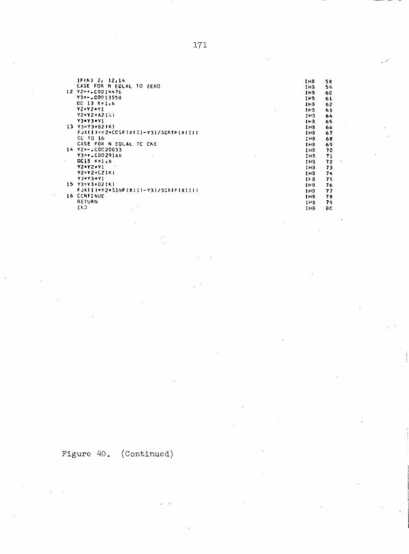
171

IF C N » 2, 12,14 CASE FOR N EQUAL TO ZERO

12 Y2=+.C0014476 Y3=-.C0013558 DO 13 K=l,6 Y2=Y2»Y1 Y2 = Y2*A2 ÎK) Y3=Y3»Y1

13 Y3 = Y3 + B2 IK) F J X CI )=Y2»CCSF(X( I) — Y3J/SCRTF fX(I)) GC TO 16 CASE FOR N EQUAL TO CNE

14 Y2=-. COC2003 3 Y3=+.C0029166 DC 15 K = 1 ,6 Y2«Y2«Y1 Y2=Y2+C2(K) Y3=Y3*Y1

15 Y3=Y3«D2(K) F J X CI)=Y2»SINF(X(I)-Y3)/SSRTF(X(I) )

16 CCNTINUE RETURN END

Figure 40. (Continued)

172.

SUBROUTINE MATINV I A ,N,B,NMAX » M, DET,INOEXl.IN0EX2, IPIVOT,P I V O T ) IHB 1 DIMENSION INOEXK1) , INDEX2(I).PIVOTtl), IPIVUT(l), All) ,8( 1 ) IHB 2 EQUIVALENCE (IROW,JROh),tICOILM, JCOLUM), IAMAX.T.SUAP), INLltNROW) IHB 3

IHB 4 INITIALIZATION IHB

IHB 5 6

10 DET= I • 0 IHB 7 15 CC 20 J=1,N 1H3 8 20 IPIVOTIJ)=0 IHB 9 30 OC 55C 1=1,N

SEARCH FOR PIVOT ELEMENT

IHB IHB fHB IHB

1C 11 12 13

40 AMAX = 0•0 IHB 14 45 OC 105 J=1,N IHB 15 50 I F (IPIVOTIJ)-l 1 60,1C5.60 IHB 16 60 CC IOC K=1,N IHB 17 70 IF !IPIVOTtK )-l ) 71, ICO,740 IHB 18 71 LL=(K-1l«NMAX*J IHB 19 80 IF (AESF(AMAX)-ABSF(A(LL))185»100,100 IHB 20 85 IROW=J IHB 21 90 ICOLUM=K IHB 22 95 AMAX=<ILL) IHB 23 100 CCNT1NUE IHB 24 105 CCNTINUE IHB 25 110 IPIVOTI IC0LUM) = IPIV0TI IC0LUMH1 IHB

IHB 26 27

INTERCHANGE RCkS TO PUT ELEMENT ON CI AGONAL IHB 28 IHB 29

130 IF ( IROW-ICCLljM) 140,260,140 IHB 30 140 OET=-DET IHB 31 150 CC 200 L = 1 » N IHB 32 151 JCON=IL-l)»NMAX IHB 33 152 NROW=JCON+IROh IHB 34 153 NC0L=JCON*ICOLUM IHB 35 160 ShAP=AlNROW) IHB 36 170 AINROW)=A(NCCL) IHB 37 200 AINCOL)=SWAP IHB 38 205 IF IM) 260 , 2 6C,21C IHB 39 210 DC 25C L = 1, M IHB 40 211 JC0N=(L-1)»NMAX IHB 41 212 NROH=JCON+IROh IHB 42 213 NCOL =JCCN +ICOLUM IHB 43 220 SWAP=BINR0W) IHB 44 230 eINROh)=B(NCOL ) IHB 45 250 B I NCOL ) = SW AP IHB 46 260 INDEX 11 I)=IROh IHB 47 270 IN0EX21 I) = ICOLUM IHB 48 271 LL = f ICOLUM-l )«NMAX+ICOLUM IHB 49 310 PIVOT I I 1=A(LL) IHB 50-320 DE T = DE T«PIVOT(I) IHB

IHB. 51 52.

DIVIDE PIVOT ROW BY PIVOT ELEMENT IHB 53 IHB 54

330 A(LL) = 1. 0 IHB 55 340 DC 350 L = 1,N IHB 56 341 NCOL=IL-1)»NMAX+ICOLUM IHB 57 350 AINCOL)=AINCOL)/PIVOT I I ) IHB 58 355 IF (Ml 371,371,360 IHB 59

Figure 4l. Matrix inversion subroutine MATINV(REVISED) (6)

173

360 DC 370 1 = 1,1* IHB 361 NC0L=(L-1)»NMAX+ICOLUP IHB 370 B(NCOLI*B(NCOL)/PlVOT(I1 IHB

IHB REOUCfc NON-PIVOT ROWS IHB

IHB 371 JC0N=(ICOLUM-1)«NtAX IHB 360 CC 55C L1=1,N IHB 390 IF IH-ICOLUM) 39 11 5 5C t 391 IHB 391 LL = JCC N+L1 IHB 400 T=A(LL) IHB 420 A(LL)=0.0 IHB 430 DC 450 L = 1,N IHB 431 NC0N=(L-1)«NMAX IHB 432 NL1 = NC0N + H IHB 433 NCOL=NCON*ICOLUK IHB 450 AlNLl)*A(NL1l-AINCOL)*T IHB 455 IF (Ml 55C,550,460 IHB 460 DO 50C L=1,M IHB 461 NCCN=(L-l)»NMAX IHB 462 NL1*NC0N+Ll IHB 46 3 NCOL=NCCN+ICOLUf IHB 500 BINLl)=B(NL1)-B(NCOL)»T IHB 550 CONTINUE . IHB

IHB INTERCHANGE CCLLPNS IHB

IHB 600 DC 71C 1 = 1,N IHB 610 L-N+l-I IHB 620 IF ( INDEXKL )-INDEX2 (L ) 16 30, 710,630 IHB 630 JR0K=INDEX 11L) IHB 64 0 JCOLUf=1NOEX2(L) IHB 641 JCON=(JROW-1)«NKAX IHB 64 2 NCDN=(JCOLUM-1)«NPAX IHB 650 CO 705 K=1,N IHB 651 NROh = JCON + K IHB 65 2 NCOL=NCON>K IHB 660 SkAP=A(NROW) IHB 670 A {NROtt ) = A ( NCOL ) IHB 700 AINCOL!=SHAP IHB 70 5 CONTINUE IHB 710 CONTINUE IHB 740 RETURN IHB

END IHB

60 61 62 6 3 6 4 6 5 66 6 7 68 6 9 7 0 7 1 7 2 7 3 7 4 7 5 7 6 7 7 7 8 7 9 80 81 8 2 8 3 8 4 8 5 86 8 7 88 8 9 9 0 9 1 9 2 9 3 9 4 9 5 9 6 9 7 9 8 9 9

100 101 102 1 0 3

Figure 4l. (Continued)

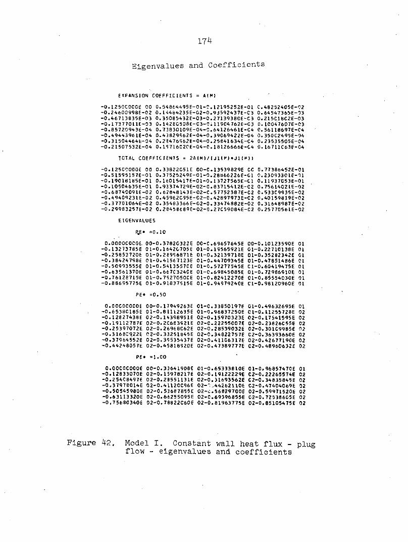
1?4

Eigenvalues and Coefficients

EXPANSION COEFFICIENTS = AIM)

-0.125QC0C0E CO 0.54864495E-01-5.12195252E-01 C.48252405E-02 -0.24600998E-0 2 0.14464235E-02-0.9 35924 37E-C3 0.64547365E-03 -0.46713835E-03 0.35085432E-03-0.2713938CE-C3 0.215C16C2E-03 -0.17377011E-03 0.14260508E-C3-C.119C4762E-C3 0.1C047607E-03 -0.85720943É-04 0.73830109E-04-C.64126461E-C4 0.56118697E-C4 -0.49443961E-04 0.43829962E-04-0.39C69422E-04 0.350C2495E-04 -0.31504464E-04 0.26476962E-04-0.25841634E-C4 0.23535505E-04 -0.21507532E-04 0.1S716020E-04-C.18126666E-G4 0.16711C63E-04

TOTAL COEFFICIENTS = 2A(M )/(J 1(M)•J 1(H)I

-0.125CCOOOE 00 0.33822051E 00-C.13539829E CC 0.77386452E-01 -0.51595157E-01 0.3 7525249E-01-0.28866226E-C1 0.23093301E-11 -0.19018185E-01 0.16015417E-01-0.13727565E-C1 0.11937C53E-01 -0.10504635E-01 0.93374729E-02-C.83715412E-C2 0.7561402IE-02 -0.6874009IE-0 2 0.62 84 614 3E-02-C.5 7752387E-C2 0.533C9935E-02 -0.49409231E-02 0.45962C95E-C2-C.42897973E-C2 0.40159819E-02 -0.37701064E-02 0.35483366E-02-0.33474 882E-02 0.31648987E-02 -0.29983257E-02 0.2 645 86 89E-02-0.27C59084E-C2 0.25770561E-02

EIGENVALUES

P*E* =0.10

0 .OOOOCOCOE. 00-0. 3782C322E 00-C. 69657645E 00-0. 10123590E 01 -0 .132 73785E 01-0. 1642G705E 01-0. 19565921E 01-0. 2271013SE 01 -0 .258537206 01-0. 289Ç6871E 01-0. 32139718E 01-0. 35282342E 01 -0 • 3 8424 798E 01-0. 41567123E 01-0. 44709345E 01-0. 47851486E 01 -0 .50993555E 01-0. 5413557CE 01-0. 57277545E Cl-0. 60419475E 01 -0 •63561370E 01-0. 667C324CE 01-0. 69845085E 01-0. 72986910E 01 -0 .76128715E 01-0. 7S27050CE 01-0. 82412270E 01-0. 85554C30E 01 -0 .88695775E 01-0. 91837515E 01-C. 94979240E Cl-0. 98120960E 01

PE» =0 .50

0 .OOOOCOCOE 00-0. 17949263E 01-C. 33850197E 01-0. 49632695E 01 -0 •6538C185E 01-0. 81112635E 01-•0. 96837250E 01-•0. 11256728E 02 -0 • 12827438E 0 2-0. 14396951E 02-•0. 15970323E 02-•0. 17541595E 02 -0 . 19112787E 02-0. 2C663S21E 02-•C. 22255007E 02-•0. 23826C55E 02 -0 •25397072E 02-0. 26968C62E 02-•0. 2 8539032E 02-•0. 301C9985E 02 -0 .3168C922E 0 2-0. 33251845E 02-•0. 34822757E C 2-•0. 363936606 02 -0 •379 64 552E 0 2-0. 3S535437E 02-•0. 411G6317E 02-•0. 42677190E 02 -0 •44248057E 02-0. 45816920E 02-•0. 47389777E C2-•0. 48960632E 02

PE* =1 .00 -

0 •OOCOCOOOE 00-•0. 33641908E 01-•0. 65333810E 01-•0. 96857470E 01 -0 .12833070E 02-0. 15978217E 02-•0. 19122229E C2-•0. 22265574E 02 -0 . 2 5408497E 02-0. 285511316 02-•0. 31693562E C2-•0. 34835845E 02 -0 .37978014E 02-•0. 4112CC96E 02- 44262110E C2-0. 474C4C69E 02 -0 .50545980E 02-0. 53687855E 02-C. 156829700E 02--0. 59971520b 02 -0 .63113320E 02-•0. 66255095E 02-C. 69396855E 02-•0. 725386C5E 02 -0 •75680340E 02-•0. 78822C60E 02-•0. 81963775E 02-•0. 85105475E 02

Figure 42. Model I. Constant wall heat flux - plug flow - eigenvalues and coefficients

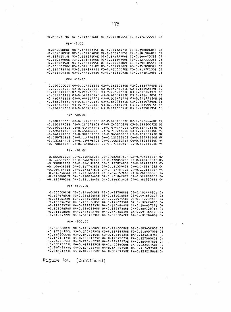
175

-0.882471706 02-0.9138886CE 02-0.94530545E G2-0.9767222CE

PE» =5.CO

0.OOCCCOCOE 00-0.1C375735E 02-C.24738573E C2-0.39880685E -0.552810356 02-0.7C796405E C2-C.86372625E C2-0.10198486E -0.11762015E 03-0.13327106E C3-0.14893306E L3-0.1646C321E -0.18C27950E C3-0.19596056E 03-0.21164540E C3-0.22733326E -0.243023586 03-0.258715956 03-0.2 7441002E C3-0.29C10555E -0.305 8C230c 03-0.3215CCV0F 03-0.33719882E C3-0.35269832E -0. 36859855E 03-0. 384299326 03-0.4C00CC70E C3-0.4157C2556 -0.4314C485E 03-0.44710752E 03-0.46281052E C3-0.47851385E

PE• =10.CC

0.OOCCCOCOE 00-0.12993625E 02-C.3615C 130E C2-0.63357595E -0.923097906 02-0.12212833E C2-C.15243C69E C2-0.18302ti19E -0.213818166 02-0.244740266 03-0,27575688E C3-0.306843376 -0.33798293E 03-0. 36916374F 03-0.4CC37723E C3-0.43161705E -0.462878356 03-0.4941575CE 03-0.52545155E 03-0.55675820E -0.588075556 C3-0.6 19402156 03-C.65C736806 C3-0.68207840E -0.71342610E 03-0.744779156 C3-C.7761370C6 C3-0.80749915E -0. 838 86500 6 0 3-0.870234356 C3-C.9C1606756 03-0.93298195E

P6* =20.CC

0.OOOOCOCOE 00-0. 141793206 02-C.443 10CCC6 C2-0.85306460E -0.133179C8E 03-0.1853734C6 03-0.240355246 C3-0.29720C72E -0.355337826 0 3-0.414399946 C3-C.474144026 C3-0.534403656 -C.595061606 03-0. 656C33256 03-0. 71 72560CE C3-0. 77868275E -0.8 4C27730E 03-0.9C2C1160E 03-0.96386335E C3-0.10258148E -0. 108785166 04-0. 114996196 04-C. 12121360E C4-0.12743660E -0.133664496 C4-0.139896706 04-0.146132766 C4-0.152372246 -0.158614786 04-0.16486C08F 04-C.17110787E C4-0.17735790E

PE* =50.OC

0.OOOOCOCOE 00-0.145966256 C2-C.482857506 02-0.99536375E -0.166439756 03-0.24669b126 0 3-0.3 3885 32 56 C3-0.440429876 -0.5500C0106 03-0.666192856 0 3-0.7 6 787 6006 C3-C.914123256 -0. 10441815E 04-0. 1 17743816 04-C. 1 3 1339436 C4-0. 14516428E -0. 15918490E 04-0. 173373676 04-C.I 877C7726 C4-0.20216796E -0.216738366 04-0.2314C5416 04-0.246157666 C4-0.26C985356 -0.2 75F80C 7E 04-0. 2 90 8 3465 6 04-C.3Cb842876 C4-0.32C899306 -0.335999206 04-0 . 35 11 384 5C 04-C.366313406 C4-0.381520856

P6 * =10C.C0

0.OOOOCOCOE 00-0. 1466CC0CE C2-0.489780006 C2-0.102449506 -0.174476506 03-0.2642960C6 03-0.3710160CE C3-0.493652C0E -0.631163506 C3-C.782489CC6 0 3-0.9465745 06 03-0.11223945E -0.130896756 04-0.150 5 36 85 6 04-0.171073506 04-0.192426856 -0.214523756 04-0.237297356 04-C.26C686856 C4-0.284637156 -0.309C9850E 04-0.334025956 04-0.3 5937 8856 C4-C.38512C75E -0.411218606 0 4-0.4376427C6 04-0.4 64 366306 C4-0.491365106 -0.516617206 54-0.5461G29C6 04-C.5738C420E C4-C.601704806

PE* =500.CO

0.OOCCCOCOE 00-0. 14675C0CE 02-C.4S2CC00CE 02-0. 10345C006 -0.17736750k 03-0.27098750E C3-C.3841875CE C3-0.51693750E -0.6692CCC0E 03-0. 84067500E C3-0.1C319 125E 04-0. 12421b75E -0.147163756 04-0. 1 72C 13756 04-C. 198758756 C4-0.227385CC6 -0.257862506 04-0.2902 36256 04-C.32443375E C4-0.3604575CE -0.398293756 04-0. 4379275C6 04-C..47934000E C4-0.522517506 -0.5*7438756 04-0.614C8675E 04-0.662447506 04-0.712497506 -0 .764218756 04-0. 817592506 04-C. ti7259750E C4-0.92921500E

0 2

02 03 03 03 03 03 03 03

02 02 03 03 03 03 03 03

02 03 03 03 04 04 14 14

02 03 03 04 n4 04 04 04

03 03 04 04 04 04 04 04

03 03 n4 04 04 04 04 04

Figure 42. (Continued)

176

PE«* PECLET NUMBER/2 = 0 .10

EIGENVALUES

0 .OOOOOOOOE 00-0. 37658935E 00-0 . 69493250E 00-0. 10107071E 01 -0 .13257228E 01-0. 164C4126E 01- 0 . 19549327E 01-0. 22693534E 01 -0 .25837108E 01-0. 28980252E 01— 0 •32123095E 01-0 . 35265716E 01 -0 .38408168E 01-0. 41550490E 01-0 . 44692710E Cl-0. 47834849E 01 -0 .50976910E 01-0. 54 118930E 01-0 . 5 7260900E 01-0. 60402830E 01

EXPANSION COEFFICIENTS: A(M)

-0 .60953966E-01 0 .422883 82E-01-0 .72094807E-02 0 .26319299E-02 -0 .12977592E-02 0 .75122387E-03-0 .48C68132E-03 0 .32946160E-03 -0 .23744226E-03 0 . 177809 13E-C3-0 .13724027E-03 0 .10855206E-03 -0 .87615370E-04 0 . 71929C61E-04-0 .59913228E-04 0 .50532466E-04 -0 .43087664E-04 0 .37093814E-04-0 .32207443E-04 0 .28183760E-04

2*A(M)/ ( J0 (M)*J0(M))=TOTAL COEFFICIENT

-0 .12190793E 00 0 .52138631E OO-O.16008712E 00 0 .84420960E-01 -0 .54435269E-01 0 .38924890E-01-0 .29650805E-01 0 .23574490E-01 -0 .19333548E-01 0 .16232876E-01-0 .13883697E-01 0 .12052866E-01 -0 .10592932E-01 0 .94063271E-02-0 .84263093E-02 0 .76057172E-02 -0 .69104465E-02 0 .63152483E-02-0 .58012143E-02 0 .53546304E-02

ASSOCIATED COEFFICIENTS C(P) FOR M^l

0 . lOOOCOOOE 01 0 .OCOOCOOOE 00 O.OOCOOOOOE 00 0 .OOOOOOOOE 00 0 .00 E 00 0 .00 E 00 0 .00 E 00 0 .00 E 00 0 .00 E 00 0 .00 E 00 0 .00 E 00 0 .00 E 00 0 .00 E 00 0 .00 E oc 0 .00 E 00 0 .00 E 00 0 .00 E 00 0 .00 E 00 o . co E 00 0 .00 E 00 0 .00 E 00 o .oc E 00 0 .00 E 00 0 .00 E 00 0 ,00 E 00 0 .00 E 00 0 .00 E 00 0 .00 E 00 0 .00 E 00 0 .00 E 00 0.00 E 00 0 .00 E 00

ASSOCIATED COEFFICIENTS C C P I FOR M=2

-0 .56683213E-02 0 .10C00000E 01 0 .63022088E-02-0 .81336961E-03 0 .246 86772E-03-0 .1C468854E-03 0 .53287028E-04-0 .30464183E-04 0 .18884074E-04-0 .12427647E-04 0 .85651690E-05-0 .61243169E-05 0 .45125549E-05-0 .34C91676E-05 0 .26306642E-05-0 .20671183E-05 0 .16500746E-05-0 .13354645E-05 0 .10940928E-05-0 .90612070E-06 0 .75777165E-06-0 .63928453E-06 0 .54362054E-C6-0 .46562272E-06 0 .40145782E-06-0 .34823907E-06 0 .30376591E-06-0 .26634265E-06 0 .23464914E-06-0 .20764 789E-06 0 .18451667E-C6-0 .16459960E-06

ASSOCIATED COEFFICIENTS CIP> FOR M=3

0 .71013497E-03-0 .64349661E-02 0 .10000000E 01 0 .63951336E-02 -0 .80801881E-0 3 0 .24632873E-03-0 .10589759E-03 0 .54807812E-04 -0 .31869823E-04 0 .20077690E-04-0 .13412781E-04 0 .93717769E-05 -0 .67851871E-05 0 .5C564741E-05-0 .38596338E-05 0 .30063203E-05 -0 .238 25955E-05 0 .19168473E-05-0 .15625517E-05 0 .12886177E-05 -0 .10737467E-05 0 .90302819E-06-0 .76581917E-06 0 .65439057E-06

Figure 43. Model II., Constant wall heat flux - fully-developed laminar flow - eigenvalues and coefficients

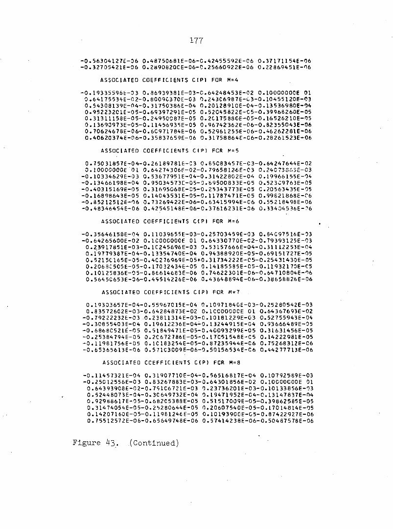
177

-0 .56304127E-06 0 .48750681E-06-0 .42455592E-C6 0 . 37171154E-06 -0 .32705421E-06 0 .2890820CE-06-C.2 5660922E-06 0 .22869451E-16

ASSOCIATED COEFFICIENTS CtP) FOR M=4

-0 . 19335596E-03 0 .86939381E-03-0 .64248453E-02 0 .LOOOOOOOE 01 0 .64175 534E -0 2-0 .8009C370E-03 0 .243C6987E-C3-0 .10455120E-03 0 .54308139E-04-0 .31750386E-04 0 .20128910E-C4-0 .13536980E-04 0 .95223201E-05-0 .69397291E-05 0 .52C45822E-C5-0 . 39968260E-05 0 .31311158E-0 5 -0 .2495C087E-05 0 .2C17588CE-05-0 .16 526210E-05 0 . 13690973E-05-0 . 11456935E-05 0 .96742362E-06-0 .82355043E-06 0 .70624678E-06-0 .6C971784E-06 0 .52961255E-06-0 .46262281E-06 0 .40620374E-06-0 .35837659E-06 0 .31758 864E-C6-0 .28 261523E-06

ASSOCIATED COEFFICIENTS C(P) FCR M=5

0 .75031857E-04-0 .26189781E-03 0 .85C83457E-C3-0 .64247644E-02 O. IOOOOOOOE 01 0 .64274306E-02-0 . 7965812-6E-03 0 .24C73863E-03

-0 . 10334629E-03 0 . 53677951E-04-0 .31422802E-04 0 .19966155E-04 -0 .13466198E-04 0 .95034573C-05-0 .69500833E-05 0 .523C9763E-05 -0 .403 15169E-05 0 . 31695068E-05-0 .25343773E-05 C .P0563435E-95 -0 .16898643E-05 0 .14043531E-05-C.11787471E-05 0 .99621868E-C6 -0 .85212512E-06 0 .73269422E-06-0 .63415994E-C6 0 .55218498E-06 -0 .48346454E-06 0 .42545148E-06-0 .37616231E-06 û .33404536E-^6

ASSOCIATED COEFFICIENTS C(P) FOR M=6

-0 .3564615 .8 E-04 0 . 11039655E-03-0 . 25703459E-03 0 . 840975 16E-03 -0 .642 65600E-02 O. ICOOCOOOE 01 0 .64330770E-C2-0 .79393125E-03

0 .2 .3917851E-03-0 . 1C245696E-03 0 . 5 3157666E-04-0 .311122 53E-04 0 .19779387E-04-0 .13354740E-04 0 .94388920E-05-0 .69151727E-05 0 .5 215C165E-0 5 -0 .4C2 76969E-05>0 .31734222E-C5-0 .25431430E-05 0 .2068C505E-05-0 . 17032434E-05 0 . 14185585E-C5-0 . i l932170E-C5 0 .1012 5836E-05-0 .86614683E-06 0 .74622301E-06-0 .64710804E-06 0 .5 64 5C65 3E-0 6 -0 .4S514226E-06 0 .4364 8894E-06-0 . 38658826E-06

ASSOCIATED COEFFICIENTS C(P) FOR M=7

0 .19303657E-04-0 .83572602E-03-

-0 .792 22232E-0 3 -0 .30855403E-C4 -0 .6868C521Ë-05 -0 .25384794E-05 -0 .11981756E-05 -0 .65365613E-06

0 .55967015E-04 0 .64284873E-02 0 .23811314 E-03-0 . 19612236E-04 0 . 5 1 849471E-05 0 .2C672786E-05 0 .1C 183254E-05 0 .571C3009E-06

0 .1097184CE-0- . ÎCOOOOOOE C . 10181229E-0 . 13244915E-0 .4C093299E-0 . 17C51548E-

-0 .87235944E--0 . 50 156534E-

0 3 -0 .25280542E-03 01 0 .64 367693E-02 03 0 .52755943E-04 04 0 .93666489E—95 05 0 .31631456E-05 05 0 .14222981E-05 06 0 .75268312E-06 06 0 .44277713E—06

ASSOCIATED COEFFICIENTS CtP) FCR M=8

-0 .11457321E-04 0 .31907710E-04-0 .56516817E-04 0 .10792589E-03 -0 .250 12556E-03 0 .83267883E-03-0 .64 301856E-02 O. IOOOOOOOE 01

0 .64393908E-02-0 .7S1C6721E-03 0 .23736201E-03-0 .10133856E-03 0 .5 2448073E-04-0 .30649732E-04 0 .19471952E-C4-C.13147837E-04 0 .92988617E-05-0 .68205388E-05 0 .51517009E-05-0 .39862585E-05 0 .314 74054E-0 5 -0 .2 52 80644E-05 0 .20607540E-05-0 .17014814E-95 0 .14207160E-05-0 .11981246E-05 0 .10193900E-C5-0 .87422927E-06 0 .75512572E-06-0 .65649748E-06 0 .57414238E-06-0 .50487578E-06

Figure 43. .(Continued)

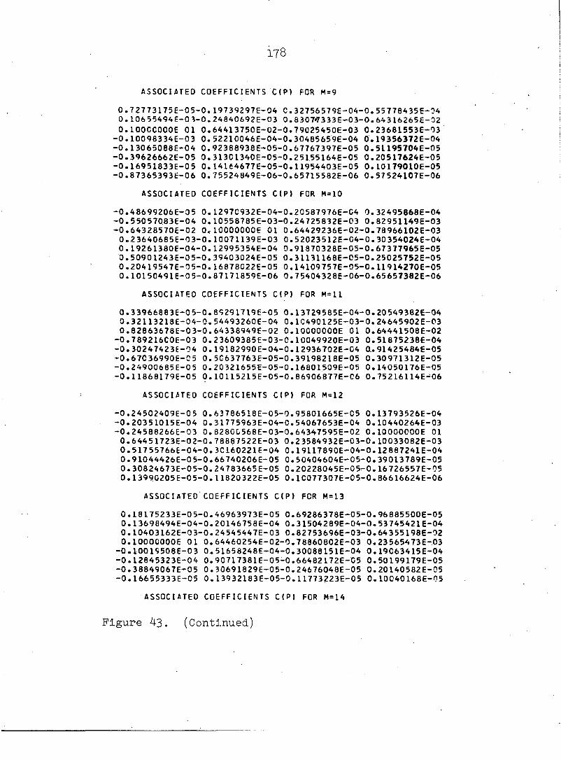
178

ASSOCIATED COEFFICIENTS C(P) FOR M=9

0 .72773175E-05-0 . 19739297E-04 0 .32756579E-04-0 . 55770435E-04 0 .106 55494E-0 3 -0 .24 840692E-03 0 . 8307 '7333E-03-0 . 643 16265E-02 O. IOOCCOOOE 01 0 .64413750E-02-0 .79025450E-03 0 .23681553E-03

-0 .10098334E-03 0 .52210046E-04-0 .30485659E-04 0 .19356372E-04 -0 .13065088E-04 0 .92388938E-05-0 .67767397E-05 0 .51195T04E-05 -0 .39626662E-05 0 .313C1340E-05-0 .25155164E-05 0 .20517624E-05 -0 .16951833E-05 0 . 14164677E-05-0 .11954403E-05 0 .10179010E-05 -0 .87365393E-06 0 .75524849E-06-0 .65715 582E-06 0 .57524107E-06

ASSOCIATED COEFFICIENTS C(P) FOR M=10

-0 .48699206E-05 0 .1297C932E-04-0 .20587976E-04 0 .32495868E-04 -0 . 550570 .83E-04 0 . 10558785E-03-0 .24725832E-03 0 .82951149E-03 -0 .64328570E-02 OdCOOOOOOE 01 0 .64429236E-02-0 .78966102E-03

0 .23640685E-03-0 .10071139E-03 0 .52023512E-C4-0 .30354024E-04 0 .19261380E-04-0 .12995354E-04 0 .91870328E-05-0 .67377965E-05 0 .50901243E-05-0 .39403024E-05 0 .31131168E-05-0 .25025752E-05 0 .20419547E-0 5 -0 .16 878C22E-05 0 .14109757E-05-0 .11914270E-05 0 .10150491E-05-0 .87171859E-06 0 .7 5404328E-06-0 .65657382E-06

ASSOCIATED COEFFICIENTS C(P) FOR M=l l

0 . 33966883E-05-0 .8S291719E-05 0 .13729585E-04-0 .20549382E-04 0 .32113218E-04-0 .54493260E-04 0 .10490125E-03-0 .24645902E-03 0 .82863678E-03-0 .64338949E-02 O. IOOOOOOOE 01 0 .64441508E-02

-0 .789216C0E-03 0 .23609385E-03-0 .10049920E-03 0 .51875238E-04 -0 .30247423E-04 0 . 19182990E-04-0 . 12936702E-G4 0 . .91425484E-05 -0 .67C36990E-C5 0 .5G637763E-05-0 .39198218E-05 0 .30971312E-05 -0 .24900685E—05 0 .20321655E-05-0 .16801509E-05 0 .14050176E-05 -0 .U868179E-05 0 . 10 115215E-05-0 . 86906 877E-C6 0 .75216114E-06

ASSOCIATED COEFFICIENTS C(P) FOR M=12

-0 .24502409E-05 0 .63786518E-05-0 .95801665E-05 0 .13793526E-04 -0 .20351015E-04 0 .31775963E-04-0 .54067653E-04 0 .10440264E-03 -0 .24588266 E-03 0 . 8280C,568 E-03-0 . 64347595E-02 O. IOOOOOOOE 01

0 .64451723E-02-0 .78887522E-03 0 .23584932E-03-0 .10033082E-03 0 .517 55766E-04-0 .30160221E-04 0 .19117890E-04-0 .12887241E-04 0 .91044426E-05-0 ,66740206E-05 0 .50404604E-05-0 .39013789E-05 0 .30824673E-05-0 .24783665E-05 0 .20228045E-0 5 -0 .16 726557E-05 0 .13990205E-05-0 .11820322E-05 0 .1C077307E-05-0 .86616624E-06

ASSOCIATED COEFFICIENTS C(P) FOR M=13

0 .18175233E-05-0 .46963973E-05 0 .69286378E-05-0 .96 885500E-05 0 .13698494E-04-0 .20146758E-04 0 .31504289E-04-0 ,53745421E-04 0 .10403162E-03-0 .24 545447E-03 0 .82753696E-03-0 .64 355198E-02 O. IOOOOOOOE 01 0 .64460254E-02-0 .78860802E-03 0 .23565473E-03

-0 .10019508E-03 0 .51658248E-04-0 .30088151E-04 0 .19063415E-04 -0 .12845323E-04 0 .90717381E-05-0 .66482172E-05 0 .50199179E-05 -0 .38849067E-05 0 .30691829E-05-0 .24676048E-05 0 .20140582E-05 -0 .16655333E-05 0 . 139 32183E-05-0 .11773223E-05 0 .10040168E-05

ASSOCIATED COEFFICIENTS C(P) FCR M=14

Figure 43. (Continued)

179

-0 .13802590E-05 0 .35458320E-05-0 .51589032E-05 0 .70526594E-05 -0 .9^524940E-05 0 .13574993E-04-0 .19969796E-04 0 .31289599E-04 -0 .53490144E-04 0 .1C374913E-03-0 .24512816E-03 0 .82718106E-03 -0 .64361777E-02 O. IOOOOOOOE 01 0 .64467531E-02-0 .7883956?E-03

0 .23549751E-03-0 .1C008419E-03 0 .51577735E-04-0 .30028012E-04 0 .19017475E-04-0 .12809601E-04 0 .90435696E-05-0 .66257534E-05 0 .50018386E-05-0 .38702479E-05 0 .30572254E-05-0 .24 578038E-05 0 .20059966E-ns -O. 1658b887E-05 C .1387753OE-C5-0 . IL 729 565E-15

ASSOCIATED COEFFICIENTS C{P) FCR M=15

0 .10694487E-05-0 .27346740E-05 0 .39350039E-05-0 .52842895E-35 0 .70504198E-05-0 .95793000E-05 0 .13458359E-04-0 .19823496E- n 4 0 .31119666E-04-0 .5 3 30 5336E-04 0 .10352955E-03-0 .24487427E-03 0 .8 269C433E-0 3 -0 .64 36 7514É-02 O. IOCCOCOOE Cl C .64473798E-12

-0 .78822354E-33 0 . 23536864E-03-0 .9 ' ^992478E-04 0 .51 5 10554E-04 -0 .29977374E-04 0 .18 97844CE-04-0 .12 778 976E-C4 C .90192014E-05 -0 .66061431E-05 0 .4995 9126E-05-0 .38572157E-05 0 .30464954E-05 -0 .24489280E-05 0 .19986316E-05-0 .16527 863E-C5 0 .13828584E-C5

ASSOCIATED COEFFICIENTS C(P) FOR M=16

-0 .84312477E-06 0 .21478786E-05-C.3C631882E-C5 C .40548863E-15 -0 .53012201E-05 0 .7009 1444E-0 5 -0 .9 502142 8E-C5 0 . 13357074E-04 -0 .19703974E-04 0 .3C984020E-04-0 .53152623E-04 0 .10335586E-33 -0 .24467295E-03 0 .82668533C-03-0 .64372576E-G2 O. IOCCOCOOE 01

0 .644 79249E-02-0 .788C8230E-03 0 .2 3526179E-C3-0 .99915822E-04 0 .51453938E-04-0 .29934372E-04 0 .18945039E-04-0 .12752563E-04 0 .8998C230E-05-0 .65889693E-05 0 .49718565E-05-0 .38456259E-05 0 .30368835E-05-0 .24409250E-05 0 .19919773E-C5-0 .16474624E-C5

ASSOCIATED COEFFICIENTS C(P J FOR M=17

0 .67483417E-C6-0 .17138767E-05 0 .24 264323E-C5-0 .3174 5 376E-05 0 .40823034E-05-0 .528C4389E-05 0 .69583735E-C5-0 .94313058E-05 0 . 13271541E-04-0 . 19 6C62 74E-04 0 . 30874577E-04-0 . 53 0 29970E- r 4 0 .103 2162 8E-0 3 -0 .244 51C92F-0 3 0 .82 651046E-C3-0 .643 77245E-02 0 . lOCOCOOOE 01 0 .64 4 83797E-0 2 -0 .7b796420E-C3 0 .23517210E-03

-0 .99851C30E-04 0 .51405784E-04-0 .29897556E-04 0 . 18916250E-^4 -0 . 12729650E-04 0 .89 79 5 302E-0 5 -0 . 6 5 738737E-C5 0 .49594238E-05 -0 .38353131E-05 0 .3C282897E-05-0 . 24337756E-C5 0 .19863065E-05

ASSOCIATED COEFFICIENTS C(P) FOR M=18

-0 .54737895E-06 0 .13866322E-05-0 .19512629E-C5 0 .25282160E-05 -0 .32C72292E-05 0 .4C747493E-05-0 .52475847E-C5 0 .69085766E-05 -0 .93693115E-05 0 . 1 3 199884E-04-0 . 19 52594CE-04 0 .30785272E-04 -0 .52930029E-04 0 . IC31C236E-03-3 .244378 18E-03 0 .82636624E-33 -0 .64381119E-0 2 0 . ICO F 01 0 .64488 1 15E-02-0 . 78786710E-03

0 .23509647E-03-0 .99795962E-04 0 .51364580E-04-0 .29865655E-04 0 .18891310£-34-0 .127C9682E-04 0 .d9633188E-05-0 .656C5685E-05 0 .49484116E-15-0 .3826 1502E-05 3 .3C206843E-05-0 .24278354E-05

ASSOCIATED COEFFICIENTS C(P) FCR M=19

Figure 43. (Continued)

180

0 .44927445E-06-0 .11356730E-05 0 . 15900C56E-05-0 .20434751E-05 0 .25630461E-05-0 .32082008E-05 0 .4C542145E-05-0 .52125891E-D5 0 .686 32 569E-05-0 .9 316044 7E-05 0 .13139850E-04-0 .194 594066-04 0 .30711624E-04-0 .52847656E-04 0 . 10 300 835E-C-3-0 . 24426842E-13 0 .82624758E-03-0 .64384722F-C2 O. IOOOOOOOE Cl 0 .54491969E-12

-0 . 787764576-03 0 . 2 3 5C 3188 E-0 .3 -C . 99748710E-04 0 .51329Ù28E-04 -0 .29638361E-04 0 .18869575E-04-C.12692187E-04 0 .89490526E-C5 -0 .65488163E-05 0 .49386695E-05-0 . 38181054E-05 0 .30 145524E-C5

ASSOCIATED COEFFICIENTS C (P ) FCR M. = 2C

-0 .37266543E-C6 0 . 9403C9 7CF-06-0 . 13108249E-05 0 .16731425E-05 -0 .207H5658E-05 0 .25694543E-05-0 .3 1962058E-05 0 .40297744E-05 -0 .51792885E-05 0 .68232526E-05-0 .92705413E-C5 0 .13C89363F-04 -0 .19403840E-04 0 .30650268E-04-0 .52779022E-C4 0 .10292988Ê-03 -0 .244176636-03 0 .82614929E-03-0 .64387997E-02 0 .100 E 01

0 .644 95335E—02—0.78771395E-03 0 .2 3497A36E-03-0 .99707849E-04 0 .5 1298145E-04-0 .29814381E-04 C. 18850529E-04-0 .12676806E-04 0 .89364766E-05-0 .65384592E-05 9 .4 9301899E-0 5 -0 .38118816E-05

PE» = PECLET NUMBER/2 = l .CO

EIGENVALUES

0 .OOOOOOOOE 00-0 .32435472E Ol -C .63885085E 0 1 -0 .95334075E 01 -0 .12677149E 02-0 .1582C175E 02-0 .18962777E 02-0 .22105114E 02 -0 .25247278E 02-0 .28389319E 02-0 .31531275E 02-0 .34673168E 02 -0 .37815012E 02-0 .40956817E 02-0 .44098594E 02-0 .47240346E 02 -0 .50382070E 02-0 .53523790E 02-C.56665490E 02-0 .598C7185E 02

EXPANSION COEFFICIENTS^ AIM)

-0 .48590124E-0I 0 .41404629E-01-0 .810G0227E-C2 0 .29108310E-02 -0 .14045933E-02 0 .8C025417E-03-0 .50630341E-C3 0 .34417224E-03 -0 .2465C431E-03 0 .18370385E-03-0 .14124410E-03 0 .11136898E-03 -0 .89656177E-04 0 .73445C09E-04-C.61064048E-04 0 .51423607E-04 -0 .43791277E-04 0 .37 662155E-04-0 .32684759E-04 0 .28648688E-04

2» A IP ) /tJO(M )»JO(M) )=TOTAL COEFFICIENT

-0 .97180248E-01 0 .51049025E 00-0 .17986168E CO 0 .93366905E-01 -0 .58916482E-01 0 .41465409E-01-0 .31231302E-01 0 .246271C4E-01 -0 .20071418E-01 0 .16771028E-01-0 .14288739E-01 0 .12365638E-01 -0 .10839670E-01 0 .96045707E-02-0 .65881628E-02 0 .77398440E-02 -0 .70232927E-02 0 .64120087E-02-0 .58871886E-0 2 0 .54429620E-02

ASSOCIATED COEFFICIENTS C(P > FOR M=1

0 .10000000E 01 O.OCOOOCOOE 00 0 .OOOOOOOOE 00 O.OOCCOOOOE 00 0 .00 E 00 0 .00 E 00 C .00 E 00 0 .00 E 00 0 .00 E 00 0 .00 E 00 0 .00 E 00 0 .00 E 00 0 .00 E uo o .oc E 00 C .00 • E 00 0 .00 E 00 0 .00 E 00 o .oc E 00 0 .00 E CO 0 .00 E 00 0 .00 E 00 0 .00 E 00 0 .00 E CO 0 .00 E 00 0 .00 ' E 00 0 .00 E 00 0 .00 E CO 0 .00 E 00 0 .00 E 00 o .oc E CO 0 .00 E 00 0 .00 E 00

Figure 43. (Continued)

181

ASSOCIATED COEFFICIENTS CIP) FOR M=2

-0 .51C27637E-01 O. IOOOOOOOE 01 0 .56647636E-01-0 .65863076E-02 0 .21020369E-C2-0 .91487356E-03 0 .47272460E-C3-0 .27281016E- r i 3 0 .17017064E-03-0 .1124 7989E-03 0 .77767327E-G4-0 .55737465E-04 0 .41143450E-04-0 .31127529E-04 0 .24046666E-04-0 .18912749E-04 0 .15108510E-04-0 .12235555E-04 0 .10029395E-04-0 .83100238E-05 0 .69521899E-05-0 .58670739E-05 0 .4 9905506E-C5-0 .42755924E-05

.0 .36872155E-0 5 -0 .31990537E-05 0 .27909964E-05-0 .24475385E-05 0 .21566029E-05-0 .19086976E-05 0 .16963069E-C5-0 .15135161E-05

ASSOCIATED COEFFICIENTS CIP) FOR M=3

0 .82180241E-02-0 .6CC61373E-01 O. ICCOOOOOE 01 0 .60143366E-01 -0 .65C 17272E-02 0 .21136429E-02-0 .94014 95 5E-03 0 .49676155E-03 -0 .29279416E-03 0 .18618653E-03-0 .12521759E-03 0 .87928901E-04 -0 .639032236-04 0 .4776369CE-04-0 .36544502E-C4 0 .28519380E-04 -0 .22637915E-04 0 . 18236388E-04-0 .14881966E-04 0 .12284355E-04 -C .10244112E-04 0 .86212544E-05-0 .73156521E-05 0 .62544494E-05 -0 .53638193E-05 0 .46634404E-05-C.40627218E-05 0 .35581874E-05 -0 .31316298E-05 0 .27687S81E-05-0 .24584607E-C5 0 .21919341E-05

ASSOCIATED COEFFICIENTS CtP) FOR M=4

-0 .22633713E-C2 0 . 1C 154884E-01-2 .6C8097 '62E-01 O. IOCCOOOOE 01 0 .615662446-31-0 . 63918294E-02 C .207 86 685E-02-0 .92747472E-03 0 .49?9C725E-0 3 -0 .29 261728E-03 0 . 18752568E-C3-0 .12711585E-03 0 .89953777E-C4-0 .65861717E-04 0 .49575858E-C4-0 .38184137E-04 0 .299 85818E-04-0 .2 3941846E-04 0 .19393036E-04-0 .15907518E-04 0 .13194390E-0 4 -0 . 11052897E-04 .0 .9 3415 090E-05-0 .79 585400E-05 0 .68296924E-0 5 -0 .58998394E-05 0 .51275172E-C5-0 .44 811484E-05 0 .39364084E-0 5 -0 .34743767E-05 0 .3C802435E-05-0 .27427638E-05

ASSOCIATED COEFFICIENTS C(P) FCR M=5

0 .86204 373E-03-0 .3C514663E-02 0 .1C003 251E-01-0 .61430640E-01 0 . lOCOCOOOE 01 0 .62363588E-01-0 .63247841E-02 0 .20530319E-02

-0 .91515225E-03 0 .48676040E-03-0 .28958568E-03 0 .18614053E-03 -0 .12662399E-03 0 .89950285E-04-0 .66121746E-04 0 .49971494E-04 -0 .38641944E-04 0 .3C463382E-04-0 .24414947E-04 0 .19848244E-04 -0 .16337865E-04 0 .13596772E-04-0 .11426502E-C4 0 .96868668E-05 -0 .82769275E-05 0 .71227744E-05-0 .61694461E-05 0 .53755128E-05 -0 .47093554E-05 0 .41465862E-05-0 .36682756E-C5 0 .326C3060E-05

ASSOCIATED COEFFICIENTS C(P) FCR M=6

-0 .40184413E-03 0 . 12583705E-02-0 .29986854E-02 0 .99389058E-02 -0 .61877672E-01 O. ICOOOOOOE 01 0 .62874 314E-C1-0 .62827408E-02

0 ,20358242E-02-0 .90593505E-03 0 .4 8153047E-03-0 .28653864E-03 0 . 18435426E-03-0 . 12559242E-03 0 .89381799E-C4-0 .65841731E-04 0 .49872683E-04-0 .38656819E-04 0 .30548756E-04-0 .24542848E-04 0 .20000405E-0 4 -0 .16 50232 3E-04 0 .13765702E-04-0 .11594830E-04 0 .9851 3611E-05-0 .84355949E-05 0 .7 2744 571E-05-0 .63135564E-05 0 .55118536E-05-0 .48380172E-05 0 .42679709E-05-0 .37840689E-05

ASSOCIATED COEFFICIENTS C(P) FCR M=7

Figure 43. (Continued)

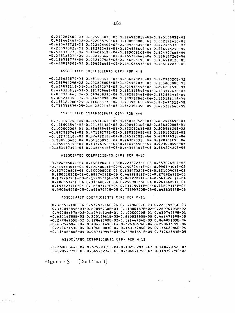
182

0 .21426768E-03-0 .62598087E-03 0 .12493081E-02-0 .29 5 5 5693E-02 0 .99144740E-02-0 .62703579E-01 O. IOOOOOOOE 01 0 .63 229141E-01

-0 .62547772E-02 0 .2G240 540E-02-0 .89922 835E-03 0 .47745537E-03 -0 .28397592E-03 0 . 1627 1C43E-03-0 .12452869E-C3 0 . 88694525E-04--0 .65403877E-04 0 .4S602613E-04-0 .3 8500610E-04 0 .30470766E-04 -0 .24518307E-04 0 .20012364E-04-0 .16538964E-04 0 .13818726E-04 -0 .11658377E-04 0 .99212796Ë-05-0 .85C89519E-05 0 .73491912E-05 -0 .63882430E-0 5 0 .55855668E-05-0 .49103653E-C5 0 .434C4287E-05

ASSOCIATED COEFFICIENTS CIP) FOR M=8

-0 .12562287E-03 0 .35169341E-03-0 .63084027E-03 0 .1229602CE-12 -0 .29296409E-0 2 0 .99C608 80E-02-0 .6244878 7E-01 0 .100CC000E 01

0 .6348S811E-01-0 .62352007E-02 0 .20157344E-C2-0 .89 429153E-03 0 .4 743206IE-0 3 -0 .2819C966E-03 0 .18131559E-C3-0 . 12357267E-03 0 .8 8C33546E-C4-0 .64945839E-04 G.492 86 546E-04-0 .38 285393E-04 0 .30327434E-0 4 -0 .24426998E-04 0 . 19958786E-C4-0 .16512811E-04 0 . 136 12498E-04-0 . 11666577E-04 0 .99398541E-05-0 .85349C32E-05 0 . 7 38 03139E-0 5 -0 .64 229 718F-05 0 . 56 2 30405E-05-0 .495 2 2 204E-35

A c. «Ï n c I a T «= [ ) r.HPFFir. IFNTS CIP) FOR M = 9

0 .79014274E-04-0 .21511961E-03 0 .36018952E-C3-0 .62244669E-03 0 .12150359E-02-0 .29138136E-02 0 .99045036E-02-0 .62639006E-01 O. IOOOOOOOE 01 0 .63689545E-01-0 .62209063E-02 0 .20096620E-02

-0 .89C58574E-03 0 .4 7189279E-03-0 .28025595E-03 0 .18016021E-03 -0 .12275110E-03 0 . ,87442218E-04-0 .64517C02E-C4 0 .48974431E-04 -0 .38058340E-04 0 .>01fc3093E-04-0 .24309332E-C4 0 .19876109E-04 -0 .16456519E-04 0 .13776192E-04-0 .11645450E-04 0 .99302649E-05 -0 .85341739E-05 0 .73864416E-05-0 .64348301E-05 0 .56427429E-05

ASSOCIATED COEFFICIENTS CIP) FOR M=10

-0 .524585C4E-04 0 .14010040E-03-0 .22382273E-03 0 .357C7650E-03 -0 .6145830 IE-03 0 .12050021E-02-0 .29C37411E-C2 0 .99059301E-02 -0 .62790680E-01 O. IOOOOOOOE 01 0 .63847329E-G1-0 .621C0907E-02

0 .20051030E-02-0 .88774592E-03 0 .46998818E-03-0 .27892693E-03 0 .1792C795E-03-0 .122C5593E-03 0 .86927824E-04-0 .64132652E-04 0 .48685345E-04-0 .3784CC77E-04 0 .29998136E-04-0 .24184891E-04 0 .19782741E-04-0 .16387149E-04 0 .13725471E-04-0 .116C9318E-04 0 .99056597E-05-0 .85187997E-05 0 .73790720E-05-0 .64383533E-05

ASSOCIATED COEFFICIENTS CIP) FOR M=l l

0 .36351418E-04-0 .95753284E-04 0 .14794607E-03-0 .22 319593E-03 0 .35285384E-03-0 .60855730E-03 0 .11980187E-02-0 .28970703E-02 0 .99086657E-02-0 .62914129E-01 O. IOOOOOOOE 01 0 .63974939E-01

-0 .62016788E-02 0 .20015961E-02-0 .88552793E-03 0 .46847339E-03 -0 .2 7784955E-03 0 . 17842C90E-03-0 .12146984E-03 0 .86485103E-04 -0 .637946C4E-04 0 .48425149E-04-0 .37638674E-04 0 .29841672E-04 -0 .24063153E-04 0 .19688083E-04-0 .16313784E-04 0 .13668986E-04 -0 .115 66366E-04 0 .98737994E-05-0 .84967651E-05 0 .737C8553E-05

ASSOCIATED COEFFICIENTS CIP) FCR M=12

-0 .26080364E-04 0 .67999315E-04-0 .10250703E-C3 0 .14847976E-03 -0 .22097975E-03 0 .34921234E-03-0 .60407179E-03 0 .11930375E-02

Figure 43. (Continued)

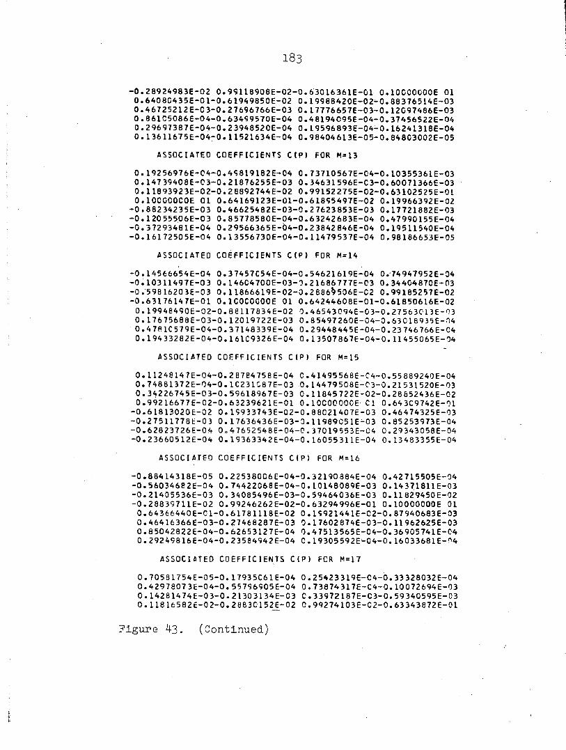
18]

-0 .28924983E-02 0 .99118908E-02-0 .63016 361E-01 O. IOCCOCOOE 01 0 .6408043 5E-01-0 .61949850E-02 0 .19988420E-02-0 .88376514E-03 0 .46725212E-03-0 .27696766E-03 0 .17776657E-03-0 .12097486E-03 0 .861C5086E-04-0 .63499570E-04 0 .48194095E-04-0 .37456522E-04 0 .29697387E-04 - 0 .23948520E-04 0 .19596893E-04-0 .16241318E-04 0 .13611675E-04-0 .11521634E-04 0 .98404613E-05-0 .848C3002E-05

ASSOCIATED COEFFICIENTS CIP) FOR M=13

0 .19256976E-04-0 .49 819182E-04 0 .73710567E-04-0 .10355361E-03 0 .14739408E-03-0 .21876255E-03 0 .346 31596E-C3-0 .60071366E-03 0 .11893923E-02-0 .28892744E-02 0 .9915227 5E-02-0 .63102525E-01 0 .1OCOCOCOE 01 0 .64169123E-01-0 .61895497E-02 0 .19966392E-02

-0 .8 82 34235E-0 3 0 .46625482E-03-0 .27623853E-03 0 .17721882E-03 -0 .120 555 .06E-03 0 .85778580E-04-0 .63242683E-04 0 .47990155E-04 -0 .37293481E-04 0 .29566365E-04-0 .23842846E-04 0 .19511540E-04 -0 .16172505E-04 0 .13556730E-04-0 .11479537E-04 0 .98186653E-05

ASSOCIATED COEFFICIENTS C(P) FOR M=14

-0 .14566654E-04 0 .37457C54E-04-0 .54621619E-04 0 .74947952E-04 -0 .10311497E-03 0 .146C4700E-03-0 .21686777E-03 0 .344C4870E-03 -0 .598 16203E-03 0 .11866619E-02-0 .2 886$506E-C2 0 .99185257E-02 -0 .63176147E-01 O. ICOCOOOOE 01 0 .64244608E-01-0 .61850616E-02 0 . 19948490E-02-0 .8e 117834E-02 0 .46543094E-03-0 .27563013E-03 0 . 17675688E-03-0 . 120 19722E-03 0 .8 5497 260E-04-0 .63 0189 35E-04 0 .47R1C579E-04-0 .37148339E-04 0 .29448445E-04-0 .23746766E-04 0 .19433282E-04-0 .161C9326E-04 0 .13507867E-04-0 .11455065E-04

ASSOCIATED COEFFICIENTS CIP) FOR M=15

0 .112 48147E-04-0 .28784758E-04 0 .41495568E-C4-0 .55889240E-04 0 .74881372E-04-0 .1C231C87E-03 0 .14479508E-C3-0 .21531520E-03 0 .34226745E-03-0 .59618967E-03 0 .11845722E-02-0 .28852436E-02 0 .99216677E-02-0 .63239621E-01 O. IOOOOOOOE CI 0 .643C9742E-01

-0 .6 1813020E-02 0 .19933743E-02-0 .88C21407E-03 0 .46474325E-03 -0 .27511778E-03 0 .17636436E-03-3 .11989051E-03 0 .85253973E-04 -0 .62823726E-04 0 .47652548E-04 -0=37019553E-C4 0=29343058E-04 -0 .23660512E-04 0 .19363342E-04-0 .16055311E-04 0 .13483355E-04

ASSOCIATED COEFFICIENTS CIP) FOR M=16

-0 .88414318E-05 0 .22538006E-04-0 .32190884E-04 0 .42715505E-04 -0 .56034682E-04 0 .74422068E-04-0 .10148089E-03 0 .14371811E-03 -0 .21405536E-03 0 .34085496E-03-0 .59464036E-03 0 .11829450E-02 -0 .28839711E-02 0 .99246262E-02-0 .63294996E-01 O. IOOOOOOOE 01

0 .64366440E-01-0 .61781118E-02 0 .19921441E-02-0 .87940683E-03 0 .46416366E-03-0 .27468287E-03 0 .17602874E-03-0 .11962625E-03 0 .85042822E-04-0 .62653127E-04 0 .47513565E-04-0 .36905741E-04 0 .29249816E-04-0 .23584942E-04 0 .19305592E-04-0 .16 033681E-04

ASSOCIATED COEFFICIENTS CIP) FCR M=17

0 .70581754E-0 5 -0 .17935C61E-04 0 .25423319E-04-0 .33328032E-04 0 .42978073E-04-0 .55796905E-04 0 .73874317E-C4-0 .10072694E-03 0 .14281474E-03-0 .21303134E-03 0 .33972187E-C3-0 .59340595E-03 0 .11816582E-02-0 .2883C152E-02 0 .99274103E-02-0 .63343872E-01

Figure 4-3. (Continued)

184

O.IOOOOOOOE 01 0 .64416G27E-01-0 .61753742E-02 0 .19911072E-02 -0 .87872438E-0 3 0 .46367109F-03-0 .27431103E-C3 0 .17574000E-03 -0 .11939754E-03 0 .84859C85E-04-0 .62503966E-04 0 .47391708E-04 -0 .368C6144E-04 0 .29169509E-04-0 .23524 80 5E-C4 0 . 192904 16E-04

ASSOCIATED COEFFICIENTS CtP) FOR M=18

-0 .5 7118519E-05 0 . 14475747E-04-0 .20391444E-04 0 .26464809E-04 -0 .33650682E-04 0 .42883341E-04-0 .55440706E-04 0 .73343738E-04 -0 .10C07160E-03 0 .142C6176E-03-0 .21219318E-03 0 .33880190E-03 -0 .59240742E-03 0 ;118C62 33E-02-0 .2 8822 807E-02 0 .99299686E-02 -0 .63386897E-01 0 . ICOOCOOOE 01 0 .64460224E-01-0 .6173C112E-02

0 .19902261E-02-0 .8 7814313E-03 0 .4 6324961E-03-0 .27399115E-03 0 .17549040E-03-0 .11919904E-03 0 .84699088E-04-0 .62 3 73988E-04 0 .47286100E-04-0 .36721846E-04 0 .2 9108453E-C4-0 .23 520814E-04

ASSOCIATED COEFFICIENTS CtP) FOR M=19

0 .46784607E-05-0 .11830578E-04 0 . I6578060E-C4-0 .213 36041E-04 0 .26813280E-04-0 .33646378E-04 0 .4 2658893E-04-0 .55067377E-04 0 .72864557E-04-0 .99 511481E-04 0 .14143371E-C3-0 .21150206E-03 0 .338C4716E—03-0 .59159068E-03 0 .11797832E-02-0 .28 817199E-02 0 .993 23590E-0 2 -0 .6 342 5480E-01 O. IOOCOOOOE Cl 0 .64499576E-01

-0 .61709445E-02 0 .19894699E-02-0 .8 7 764417E-03 C .46288663E-03 -0 .27371485E-03 0 .17527416E-03-0 . i l902676E-03 0 .84560486E-04 -0 .62262516E-04 0 .47 198561E-04-0 .36661694E-04 0 .29 122373E-04

ASSOCIATED COEFFICIENTS C(P) FOR M=20

-0 .38735164E-05 0 .97767578E-05-0 .13639379E-04 0 .17430160E-04 -0 .21689696E-04 0 .26870098E-04-0 .33515235E-04 0 .423976276-04 -0 .54715178E-04 0 .72443851E-04-0 .99035007E-04 0 .14090753E -03 -0 .21092709E-03 0 .33742141E-03-0 .59091490E-03 0 .11790925E -02 -0 .28812858E-02 0 .99 345730E-02-0 .63460011E-01 O . IOOOOOOOE 01

0 .64534941E-01-0 .61691293E-02 0 .19888184E-02-0 .87721393E-03 0 .46257300E-03-0 .27347580E-03 0 .17508713E-03-0 .11887853E -03 0 .84443094E-04-0 .62172629E-04 0 .47141869E-04-0 .36703640E -04

PE»= PECLET NUMBER/2 = 5 .00

EIGENVALUES

0 .OOOOOOOOE 00-0 .93939685E 01-0 .22719006E 02-0 .37263632E 02 -0 .52320420E 02-0 .67618060E 02-0 .83C44175E 02-0 .98546455E 02 -0 .11409757E 0 3-0 .12968192E 03-0 .14528992E 03-0 .16091535E 03 -0 .17655400E 03-0 .19220293E 03-0 .20786000E 03-0 .22352365E 03 -0 .23919267E 03-0 .25466612E 03-0 .27054332E 03-0 .286223656 03

EXPANSION COEFFICIENTS» AIM)

-0 .20516677E-0 1 0 .37632642E-01-0 .93286969E-02 0 .36183219E-02 -0 .17342711E-02 0 .95773656E-03-0 .58586373E-Ç3 0 .38655466E-03 -0 .27004123E-03 0 .19714876E-03-0 .14902 766E-03 0 .11585533E-03 -0 .92165307E-04 0 .74743903E-04-0 .61613335E-04 0 .51508939E-04 -0 .43596618E-04 0 .37315568E-04-0 .32302212E-04 0 .285129506-04

Figure 43. (Continued)

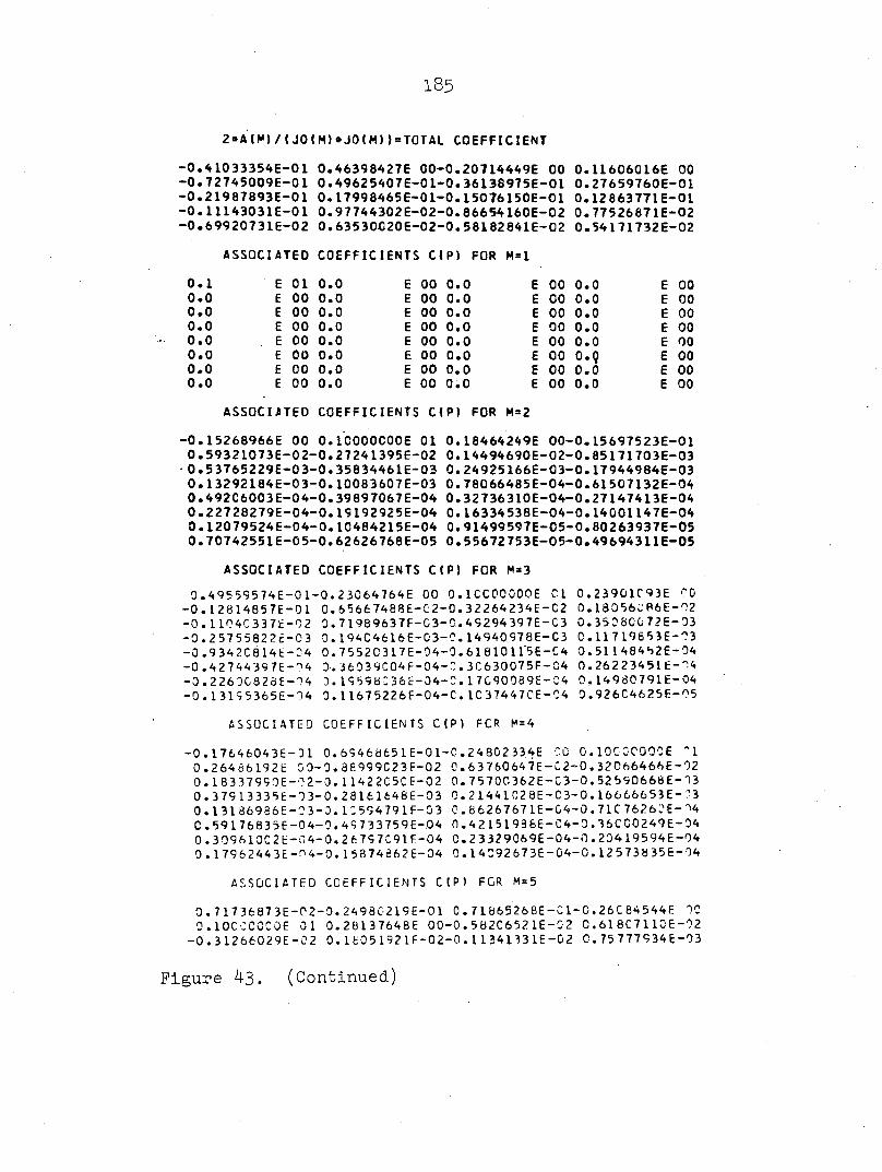
185

2»A(M)/ ( J0 IM)»J0 tM))=TOTAL COEFFICIENT

-0 .41033354E-01 0 .46398427E 00-0 .20714449E 00 0 .11606016E 00 -0 .72745009E-01 0 .49625407E-01-0 .36138975E-01 0 .27659760E-01 -0 .21987893E-01 0 .17998465E-01-0 .15076150E-01 0 .12863771E-01 -0 .11143031E-01 0 .97744302E-02-0 .86654160E-02 0 .77526671E-02 -0 .69920731E-02 0 .63530C20E-02-0 .58182841E-02 0 .54171732E-02

ASSOCIATED COEFFICIENTS CIP) FOR M=1

0 .1 E 01 0 .0 E 00 0 .0 E 00 0.0 E 00 0 .0 E 00 0 .0 E 00 0 .0 E 00 0.0 E 00 0 .0 E 00 0 .0 E 00 0 .0 E 00 0.0 E 00 0 .0 E 00 0 .0 E 00 o.o E 00 0.0 E 00 0 .0 . E 00 0 .0 E 00 0 .0 E 00 0.0 E 00 0 .0 E 00 0 .0 E 00 0.0 E 00 O.Q E 00 0 .0 E 00 0 .0 E 00 0.0 E 00 0.0 E 00 0 .0 E 00 0 .0 E 00 0.0 E 00 0.0 E 00

ASSOCIATED COEFFICIENTS CIP) FOR M=2

-0 .15268966E 00 O. IOOOOOOOE 01 0 .18464249E 00-0 .15697523E-01 0 .59321073E-02-0 .27241395E-02 0 .14494690E-02-0 .85171703E-03 0 .53765229E-03-0 .35834461E-03 0 .24925166E-03-0 .17944984E-03 0 .13292184E-03-0 .10083607E-03 0 .78066485E-04-0 .61507132E-04 0 .49206003E-04-0 .39897067E-04 0 .32736310E-04-0 .27147413E-04 0 .22728279E-04-0 .19192925E-04 0 .16334 538E-04-0 .14001147E-04 0 .12079524E-04-0 .10484215E-04 0 .91499597E-05-0 .80263937E-05 0 .70742551E-05-0 .62626768E-05 0 .55672753E-05-0 .49694311E-05

ASSOCIATED COEFFICIENTS C(P) FOR M=3

0.49559574E-01-0.23064764E 00 0.1CCOOOOOE Cl 0.23901C93E CO -0.12814857E-01 0.65667488E-C2-0.32264234E-C2 0.I8û56vB6E-02 -0.11C4C337Ë-C2 0.7198 963 7F-G3-0.4 9 294 39 7E-C3 0.3538CC72E-03 -0.25755822t-C3 0.194C4616E-03-C.14 94097 8E-C3 0.11719653E-C3 -0.9342C814E-04 0 . 7552C3 17E-04-0.61810115E-C4 0.511484b2E-04 -0.427443S7E-04 0. 36039C04 F-04-".. 3C630075F-04 0 . 26 2 2 34 51 E-14 -0.2260G828E-14 3. 1959tiC36E-04-C.17C90089E-C4 0.14980791E-04 -0.13155365E-14 0. 11675226F-04-C.IC37447CE-04 0.926C4625E-05

ASSOCIATED COEFFICIENTS C(P) FCR M=4

-0.17646043E-01 0.69468651E-01-C.2480 2334E CC O.IOCOCOOOE "1 0.264Ù6192E 03-0.36999C23F-02 0.63760647E-C2-0.32C66466E-02 0.18337990E-02-0.U422C5CE-02 0.7 570C362E-C3-0.52590666E-13 0.3 79 13335E-0 3-0.2816164 8 E-03 0 . 2 1441 02 8E -C 3-0. 166666 53 E-.">3 0. 131 86986E-03-3. 12 594791F-03 C.ti62 67671E-G4-0.71C7626:E-14 0.591768 3 5E-0 4-0.49 73 3 759E-04 0.42151936E-C4-0.36CC0249E-04 0.309610C2E-04-0.26797C91E-04 0.23329069E-04-0.20419594E-04 0.17962443E-14-0.15874862E-04 0.14C92673E-G4-0.12 5738 35E-04

ASSOCIATED COEFFICIENTS CIP) FCR M=5

0. 7 1736873E-02-0. 249802 19E-01 0. 71865268E-C1-0.26C84544E 10 0.lOCCCOCOE 01 0.28137648E 00-0.582C6521E-C2 0.618C7110E-02 -0 . 3 1266029E-C2 0. 1 605 192 IF-02-0. 1 134133 IE-G2 0. 75777934E-03

Figure 43. (Continued)

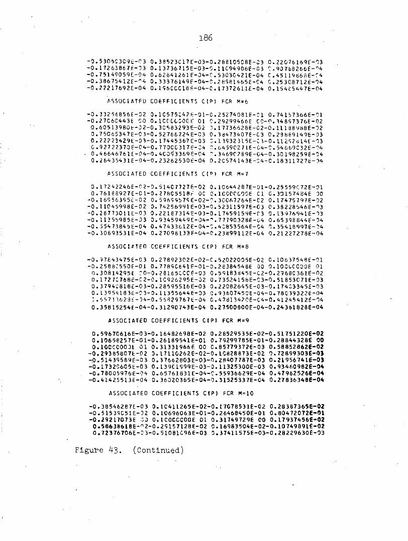
186

-0.53C5C3C9E-C3 0.38523C17E-03-0.28610508E-C3 0.22076169E-03 -0.17263867ê-0 3 0. I 3736715E-03-0. 11C94906E-03 -0.75149059E-04 0.62641261E-D4-C.5303G421E-04 -0.38675412E-"4 0.33376149F-04-0 -0 .22217692E-04 0. 1S6CCC16h-04-C

C 2H981465E-C4 C 1737261 1E-04 0

, 90 768266E-"4 , 45 1 1966SE-C4 , 253C87 12E-04 ,15 4£ 544 7E-04

ASSOCIATfD COEFFICIENTS CtP) FCR M = 6

-0.33256856E--0.27C6C443E 0.60513980fc-0.75065347E-0.22223429E-G.92722370E-0.46646761E-0.26435431E-

02 0.1C575C42E-01-00 0. 1CCXCC00E 01 0 2-0.30583293E-02 03-0.52766724E-C3 03-0.17445367E-03 C-4-0. 770003176-04 04-0.4C393369E-04 04-0.232625306-04

, 25274081E-, 29299466E , 1 7736628E-. 38473407E-, 13932315E-. 64 5902 7 IE-, 3469C289E-.2C574143E-

Cl 0.74157366E-01 CC-O.34897376E-02 O2-O.Hl 88988E-02 C 3 0.29669149E-03 C3-0. 11292614E-13 C4-C.54669C32E-04 04-0. 30 198259E-04 04-0.18311727E-04

ASSOCIATED COEFFICIENTS C t " > FCR M=7

0.17242246E-C2-0 . 76166927E-01--0.16956395E-02 -0.1 1C45998E-02 -0.2877 3011E-0 3 -0. 11355985E-D3 -0. 5 54 7 384 5 E-0 4 -0. 30693531E-04

0.514C7727E-02 0. 0. 27805518r" 00 0. 0.59699579E-02-0. 0. 74256991E-03-0. 0.22187314E-03-0. 0.93459449E-04-". 0.47433612E-04-C. 0.27096133F-G4-0.

10644287E-Û1-0. ICOCCCOOE Cl 0. 30C67264E-C2 0. 52 31159 7E-C 3 0. 17459159E-C3 0. 7 7 790 32 8E-04 0. 4C853564E-C4 0. 2 3 699112E-0 4 0.

25559C72E-01 30157464E 00 17475797E-02 38228546E-13 13976941E-13 65398844E-04 35418997 E-04 21227278E-04

ASSOCIATED COEFFICIENTS CtP) FCR M=8

-0.97643475E-03 0.27892302E-02-C.52022005E-02 0.10637548E-01 -0. 2588C550E-01 0. 778SC641E-01-0.26384548E 00 0.lOOCCCOOE 01 0. 308 14295E 00-0. 28165CCCE-0 3 0. 59183845E-C2-0.29680361E-02 0. 1 72 7C768E-C2-0.1C92 6295E-Û2 0. 73524156E-C3-0. 51853C71E-03 0.3 794C818E-0 3-0.28595516E-03 0.22082645E-03-0.17403345E-03 0.13954183E-C3-0.11355644E-03 C.9360745OE-04-0.73C39322E-04 : . 'J 5 7 1 362 3 E-04-0. 5 5829767 E-04 0.4781342 OE-C 4-0.41245412E-04 0 .358 15254E-04-0 . 31290743E-04 0 .27500800E-04 -0 .24361828E-04

ASSOCIATED COEFFICIENTS CtP) FCR M=9

0 .5967C616E-0 3 -0 . 16482698E-02 0 .2 85295 35E-02-0 .51751220E -02 0.10658257E-01-0.26189541E-01 0.79299785E-01-0.28844328E 00 0. 10CCC0C0E 01 0. 31331966E 00 C.85779372E-03 0.58852862E-02

-0 .293858C7E-02 D. 1711G262E-02-0 . IG828873E-02 0 .72899303E-03 -0.51439589E-03 0.37662803E-03-0.2 84077872-03 0.219567416-03 -0.1732C605E-03 0.139C1999E-03-0.11325300E-03 0.934609826-0* -0.78005976E-04 0.6576 1831E-04-C.55936629E-04 0.479625266-0* -0.41425513E-04 0.36020365E-04-0.31525337E-04 0.278363486-04

ASSOCIATED COEFFICIENTS CtP) FCR M=10

-0 .38546287E-03 0 .1C411265E-02-0 .17078531E-02 0 .283873656 -02 -0.51539C51E-02 0. 10696063E-01-0.26468450E-01 0.804720726-01 -0.29217073E CO 0.ICOCCCOOE 01 0.31749729E CO 0.179374566-02

0 .58638618E- 0 2-0 .29157128E-02 0 .16983504E-02-0 .107498916-02 0 .72376706E-C-3-0 . 51081C96E-03 0 .37411575E-03-0 . 28229630E-03

Figure 43. (Continued)

187

0 . 21829851E-03-0 . 17230471E-03 0 .13838648E-03-0 .11281704E-03 0 .93172145E-04-0 .77827636F-04 0 .65667093E-04-0 .559C5944E-04 0 .4 79 82278E-04-0 .41486406E-04 0 .36132375E-04-0 .31780355E-04

ASSOCIATED COEFFICIENTS C(P) FOR M=l l

0 .26083889E-03-0 .69311914E-03 0 .1C933471E-C2-0 .17046102E-02 0 .2 819 5479E-0 2 -0 .514 37984E-02 0 .10740406E-01-0 .26 714590E-01 0 .814 56678E-01-0 .29 524660E 00 O. IOOOOOOOE 01 0 .32093619E 00 0 .25755428E-02 0 .58499887E-02-0 .28976098E-02 0 .16882119E-02

-0 .10685536E-02 0 .7194 1182E-03-0 .50774684E-03 0 .37190670E-03 -0 .28067909E-03 0 .21710398E-03-0 .17141917E-03 0 . 13773077E-03 -0 .11233476E-03 0 .92822372E-04-0 .77586 302E-04 0 .655C0304E-04 -0 .55804477E-04 0 .47938385E-04-0 .41510963E-C4 0 .36344476E-04

ASSOCIATED COEFFICIENTS C(P) FOR M=12

-0 .18334017E-03 0 .48131C92E-03-0 .73747C86E-03 0 .10964063E-02 -0 .16924233E-02 0 .28050154E-02-0 .51413636E-02 0 .10785706E-01 -0 .26930410E-01 0 .82292288E-01-0 .29782475E CO O. IOOOOOOOE 01

0 .3238150IE 00 0 .32379032E-02 0 .58411029E-02-0 .288 30181E-02 0 . 16799931E-02-0 .1C632654E-02 0 .71577307E-03-0 .50513782E-03 0 .36998616E-03-0 .27924089E-03 0 .21601498E-C3-0 .17C58924E-03 0 .137G9682E-03-0 .11185148E-03 0 .92456754E-04-0 .773C8439E-04 0 .65305861E-04-0 .55679911E-04 0 .4 7896920E-04-0 .41713490E-04

ASSOCIATED COEFFICIENTS C(P) FOR M=13

0 .13299247E-03-0 .34593419E-03 0 .51847887E-03-0 .74362712E-03 0 .10897615E-02-0 . 16 811C29E-02 0 .27952515E-02-0 .51435502E-02 0 .108 29392E-01-0 .27119786E-01 0 .83009055E-01-0 .300C1634E 00 0 . lOOCCOOOE 01 0 .32625932E 00 0 .38060094E-02 0 .58355835E-02

-0 .28710707E-02 0 .16732468E-02-0 .10588823E-02 0 .71271840E-93 -0 .50291539E-03 0 .36 8 32405E-03-0 .2 7797495E-03 0 . 215039C8E-03 -0 .16983131E-03 0 .13650623E-03-0 .11139198E-03 0 .921C2427E-C4 -0 .77042085E-04 0 .65120705E-04-0 .5 5595217E-C4 0 .48122663E-04

ASSOCIATED COEFFICIENTS CIP) FCR M=14

-0 .99060621E-04 0 .25583809E-03-0 .37695533E-C3 0 .52588594E-03 -0 .74C636C2E-03 0 .1C82C605E-02-0 .16722021E-02 0 .27890566E-02 -0 .51483617E-02 0 .1C8 7C363E-01-0 .27286513E-01 0 .83629988E-01 -0 .30190118E 00 0 .1C0C0C00E 01 0 .32635991E CO 0 .42984723E-02

0 .58323719E -02 -0 . 2861 1513F-02 0 . 16676A48E -02 -0 .10 552165E-02 0 .71013858E-03-0 .5C 1C1715E-03 0 . 36688697E-03-0 .27686642E-03 0 .21417338E-0 3 -0 .16 915C43E-03 C . I3 596966E-03-0 .11097150E-03 0 . 917 80008E-04-0 . 768 12238E-04 0 .6 5C10844E-04-0 .558 79513E-04

ASSOCIATED COEFFICIENTS C(P) FCR M=15

0 .75468230E-04-0 .19381195E-03 0 .28175116E-03-0 .38462093E-03 0 .52515838E-03-0 .73572369E-03 0 .10753096E-02-0 .16655392E-02 0 .27853512E-0 2 -0 .51545789E-02 0 .1C9C82 69E-01-0 .27434046E-01 0 .84172 515E-01-0 .30 353877E 00 O. IOOOOOOOE 01 0 .33018420E 00 0 .47293669E-02 0 .5 8 3C7 577E-02-0 .28528115E-C2 0 .16629446E-02

-0 .10521248E-02 0 .7C794692E-03-0 .49939057E-C3 0 .36564419E-03 -0 .275898S2E-03 0 .21341168E-03-0 .16854779E-C3 0 .13549472E-03 -0 .11C60518E-03 0 .91518763E-04-0 .76694298E-C4 0 .65395279E-04

Figure 43. (Continued)

188

A S S O C I A T E D C O E F F I C I E N T S C ( P ) F C R M = 1 6

- 0 . 5 8 6 2 0 6 1 4 E - 0 4 0 . 1 4 9 8 6 6 2 6 E - 0 3 - 0 . 2 1 5 5 3 3 0 2 E - C 3 0 . 2 8 9 1 6 9 9 1 E - 1 3 - 0 . 3 8 5 2 4 5 4 2 E - 0 3 0 . 5 2 2 2 0 4 3 8 E - 0 3 - 0 . 7 3 0 9 1 2 3 9 E - 0 3 0 . 1 0 6 9 8 2 3 9 E - 0 2 - 0 . 1 6 6 0 6 4 3 5 E - 1 2 0 . 2 7 8 3 3 4 9 0 E - 0 2 - 0 . 5 1 6 1 4 7 6 9 E - 0 2 0 . 1 0 9 4 3 1 4 4 E - 0 1 - 0 . 2 7 5 6 5 2 7 3 E - 0 l 0 . 8 4 6 5 0 4 6 1 E - 0 1 - 0 . 3 0 4 9 7 4 8 3 E 0 0 O . I O O O O O O O E 0 1

0 . 3 3 1 7 8 2 8 7 E C O 0 . 5 1 0 9 4 3 2 4 E - 0 2 0 . 5 8 3 0 2 6 2 3 E - 0 2 - 0 . 2 8 4 5 7 2 7 1 E - 0 2 0 . 1 6 5 8 9 6 3 8 E - 0 2 - 0 . 1 C 4 9 4 9 9 0 E - 0 2 0 . 7 C 6 0 7 5 9 5 E - 0 3 - C . 4 9 7 9 9 3 3 9 E - 0 3 0 . 3 6 4 5 7 0 2 8 E - 0 3 - 0 . 2 7 5 C 5 8 9 2 E - 0 3 0 . 2 1 2 7 4 9 1 5 E - C 3 - 0 . 1 6 8 0 2 6 5 8 E - 0 3 0 . 1 3 5 0 9 4 3 4 E - 0 3 - 0 . 1 1 0 3 2 4 6 0 E - 0 3 0 . 9 1 4 1 0 6 7 2 E - C 4 - 0 . 7 7 2 3 1 5 7 5 E - 0 4

A S S O C I A T E D C O E F F I C I E N T S C ( P ) F C R M = 1 7

0 . 4 6 3 0 7 8 9 I E - 0 4 - 0 . 1 1 7 9 5 3 7 5 E - 0 3 0 . 1 6 6 1 6 0 5 I E - 0 3 - 0 . 2 2 2 4 6 7 4 4 E - 0 3 0 . 2 9 0 5 6 9 5 I E - 0 3 - 0 . 3 8 3 6 2 1 3 9 E - C 3 0 . 5 1 8 8 8 3 6 9 E - C 3 - 0 . 7 2 6 7 2 9 5 5 E - 0 3 0 . 1 0 6 5 4 8 C 5 E - 0 2 - 0 . 1 6 5 7 C 7 7 8 E - 0 2 0 . 2 7 8 2 5 0 4 0 E - C 2 - 0 . 5 1 6 8 6 2 6 3 E - 0 2 0 . 1 0 9 7 5 1 3 8 E - 0 1 - 0 . 2 7 6 8 2 6 2 4 E - 0 1 0 . 8 5 C 7 4 5 0 8 E - C 1 - 0 . 3 0 6 2 4 3 9 4 E C O 0 . 1 O O O C O C O E 0 1 0 . 3 3 3 1 9 5 1 9 E O C 0 . 5 4 4 7 1 5 8 9 E - 0 2 0 . 5 8 3 C 5 6 1 1 E - 0 2

- 0 . 2 8 3 9 6 5 2 9 E - C 2 0 . 1 6 5 5 5 6 6 5 E - 0 2 - 0 . 1 0 4 7 2 5 6 4 E - 0 2 0 . 7 0 4 4 7 3 0 7 E - 0 3 - 0 . 4 9 6 7 9 2 8 4 E - 0 3 0 . 3 6 3 6 4 6 0 5 E - 0 3 - 0 . 2 7 4 3 3 7 6 1 E - 0 3 0 . 2 1 2 1 8 6 8 l E - " 3 - 0 . 1 6 7 6 C 0 2 4 E - D 3 0 . 1 3 4 8 C 6 2 7 E - 0 3 - 0 . i l C 2 4 7 0 I E - 0 3 0 . 9 2 1 7 1 2 7 1 E - 0 4

A S S O C I A T E D C O E F F I C I E N T S C ( P ) F C R M = 1 8

- 0 . 3 7 1 2 5 6 1 3 E - 0 4 0 . 9 4 2 7 9 0 3 9 E - 0 4 - 0 . 1 3 3 4 4 5 0 6 E - 0 3 0 . 1 7 4 5 1 8 1 8 E - 0 3 - 0 . 2 2 4 2 8 2 2 1 E - 0 3 0 . 2 8 9 8 3 4 9 4 E - 0 3 - 0 . 3 8 1 3 9 0 0 3 E - 0 3 0 . 5 1 5 7 9 1 9 0 E - C 3 - 0 . 7 2 3 2 4 1 3 3 E - 0 3 0 . 1 0 6 2 C 7 0 2 E - 0 2 - 0 . 1 6 5 4 4 9 8 7 E - 0 2 0 . 2 7 8 2 4 4 4 5 E - 0 2 - 0 . 5 1 7 5 7 6 1 0 E - 0 2 0 . 1 1 0 C 4 4 7 1 E - 0 1 - 0 . 2 7 7 8 8 0 5 5 E - 0 1 0 . 8 5 4 5 3 0 9 5 E - 0 1 - 0 . 3 0 7 3 7 3 6 3 E 0 0 0 . I C O C C C O O E 0 1 0 . 3 3 4 4 5 1 7 5 E C O 0 . 5 7 4 9 1 7 4 5 E - 0 2

0 . 5 8 3 1 4 2 0 8 E - 0 2 - 0 . 2 8 3 4 4 C 2 3 E - 0 2 0 . 1 6 5 2 6 4 9 6 E - C 2 - 0 . 1 0 4 5 3 3 3 G E - 0 2 0 . 7 0 3 0 9 9 3 7 E - 0 3 - 0 . 4 9 5 7 6 6 2 9 E - 0 3 0 . 3 6 2 8 6 0 9 7 E - C 3 - 0 . 2 7 3 7 3 6 2 9 E - 0 3 0 . 2 1 1 7 4 1 7 4 E - 0 3 - 0 . 1 6 7 3 1 7 8 4 E - 0 3 0 . 1 3 4 7 8 5 3 4 E - 0 3 - 0 . 1 1 1 3 2 9 5 8 E - 0 3

A S S O C I A T E D C O E F F I C I E N T S C ( P ) F O R M = 1 9

0 . 3 0 1 5 4 9 9 2 E - 0 4 - 0 . 7 6 3 8 4 4 1 3 E - 0 4 0 . 1 0 7 4 7 0 9 2 E - Q 3 - 0 . 1 3 9 2 1 C 7 2 E - 0 3 3 . I 7 6 5 2 6 0 7 E - 0 3 - 0 . 2 2 4 1 3 6 4 4 6 - 0 3 C . 2 8 8 3 8 5 9 5 E - C 3 - 0 . 3 7 9 1 4 4 5 0 E - 0 3 0 . 5 1 3 C 9 2 8 3 E - 0 3 - 0 . 7 2 0 3 7 9 0 4 E - 0 3 C . 1 0 5 9 3 9 t i ' 6 E - C 2 - 0 . 1 6 5 2 6 5 4 3 E - 0 2 0 . 2 7 8 2 9 2 C 0 E - 0 2 - 0 . 5 1 8 2 7 3 7 5 E - 0 2 0 . 1 1 0 3 1 3 9 8 E - C 1 - 0 . 2 7 8 8 3 2 5 D E - 0 1 0 . 8 5 7 9 3 1 1 4 E - 0 1 - 0 . 3 0 8 3 8 5 3 5 E 0 0 O . I O O O O O O O E 0 1 0 . 3 3 5 5 7 8 " » E 0 0 0 . 6 0 P C 9 5 8 1 E - 0 2 0 . 5 8 3 2 6 7 1 8 E - 0 2 - 0 . 2 8 2 9 8 3 4 5 E - 0 2 0 . 1 6 5 C 1 3 4 9 E - 0 2

- 0 . 1 0 4 3 6 8 3 1 E - 0 2 0 . 7 C 1 9 2 9 2 8 E - 0 3 - 0 . 4 9 4 9 0 2 6 8 E - 0 3 0 . 3 6 2 2 1 9 0 4 E - C 3 - 0 . 2 7 3 2 7 9 4 8 E - C 3 0 . 2 1 1 4 8 1 1 2 E - 0 3 - 0 . 1 6 7 3 8 9 C 5 E - 0 3 0 . 1 3 6 3 3 3 C 2 E - 0 3

A S S O C I A T E D C O E F F I C I E N T S C ( P ) F O R M = 2 0

-0 .2 4 7 7 9 1 7 0 E - 0 4 0 . 6 2 6 3 3 9 4 6 E - 0 4 - 0 . 8 7 6 8 1 6 5 4 E - 0 4 0 . 1 1266813E - 0 3 - 0 . 1 4 1 2 7 5 8 3 E - 0 3 0 . 1 7 6 7 6 4 8 7 E - 0 3 - 0 . 2 2 3 2 4 5 2 8 E - C 3 0 . 2 8 6 7 7 8 4 9 E - 0 3 - 0 . 3 7 7 0 9 1 0 4 E - 0 3 0 . 5 1 0 7 9 7 8 6 E - 0 3 - 0 . 7 1 8 0 4 3 2 2 E - C 3 0 . 1 0 5 7 3 0 6 5 E - 0 2 - 0 . 1 6 5 1 3 5 9 5 E - 0 2 0 . 2 7 8 3 7 5 8 5 E - 0 2 - 0 . 5 1 8 9 4 7 5 3 E - 0 2 0 . 1 1 0 5 6 1 6 1 E - C 1 - 0 . 2 7 9 6 9 5 9 9 E - 0 1 0 . 8 6 I C O 1 8 0 E - 0 1 - 0 . 3 0 9 2 9 6 4 2 E C O O . I O O O O O O O E 0 1

0 . 3 3 6 5 9 2 6 7 E 0 0 0 . 6 2 6 6 7 8 2 2 E - 0 2 0 . 5 8 3 4 2 1 6 8 E - 0 2 - 0 . 2 8 2 5 8 4 9 9 E - 0 2 0 . 1 6 4 7 9 7 0 2 E - 0 2 - 0 . 1 C 4 2 2 8 1 6 E - 0 2 0 . 7 0 C 9 5 5 3 7 E - 0 3 - 0 . 4 9 4 2 1 3 3 0 E - 0 3 0 . 3 6 1 7 5 8 2 3 E - 0 3 - 0 . 2 7 3 0 6 2 8 8 E - 0 3 0 . 2 1 1 6 9 6 0 2 E - C 3 - 0 . 1 6 9 6 1 7 3 7 E - 0 3

Figure 43. (Continued)

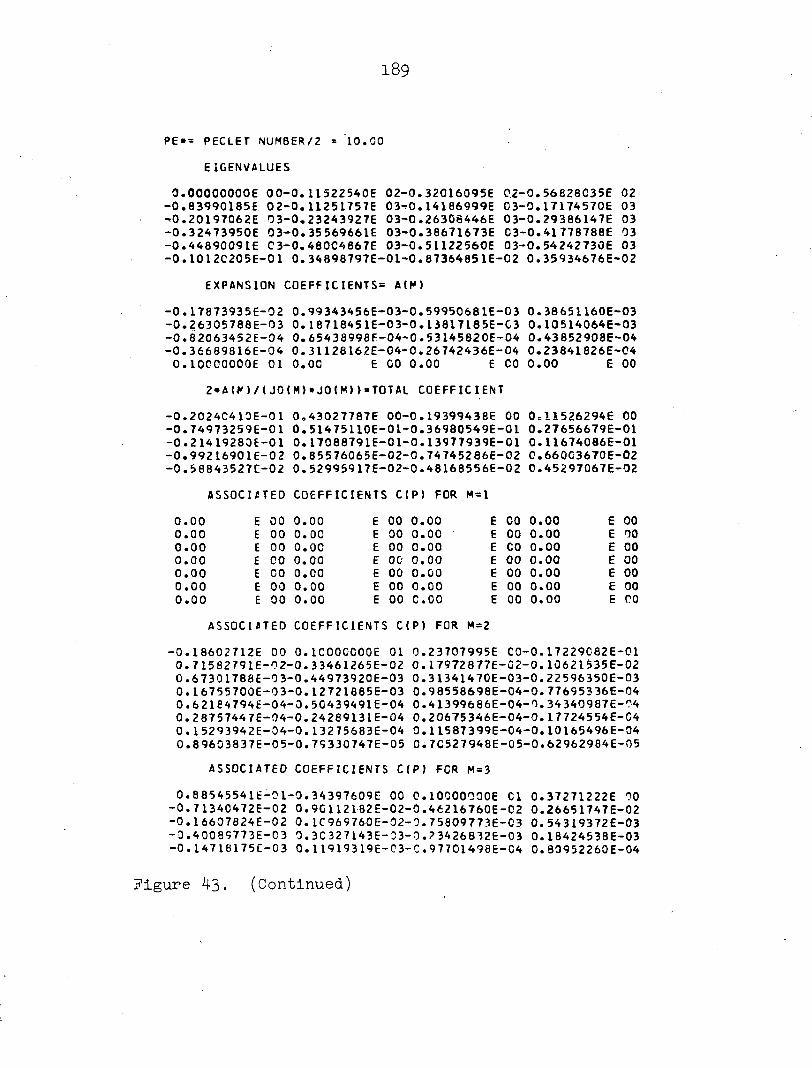
189

PE» 3 PECLET NUMBER/2 = 10 .00

E IGENVALUES

0 .OOOOOOOOE 0 0 --0 .83990185E 0 2-t0 .20197062E 0 3--0 .32473950E 03--0 .44890091E C3--0 .1012C205E-01

0 . 11522540E 0 .11251757E 0 .23243927E 0 .35 569661E 0 .480C4867E 0 .34898797E-

02-0 .32016095E 03- r0 .14186999E 03-0 .26306446E 03-0 .38671673E 03-0 .51122560E 01-0 .8736485 IE-

02-0 .56828C35E 02 C3-0 .17174570E 03 03-0 .29386147E 03 03-0 .41778788E 03 03-0 .54242730E 03

•02 0 . 35934676E-02

EXPANSION COEFFICIENTS: AIM)

-0 .17873935E-02 0 .99343456E-03-0 .59950681E-03 0 .38651160E-03 -0 .26305788E-03 0 .18718451E-03-0 .13817185E-C3 0 .10514064E-03 -0 .82063452E-04 0 .654 38998E-04-0 .53145820E-04 0 .43852908E-04 -0 .3 6689816E-04 0 .31128162E-04-0 .26742436E-04 0 .23841826E-04

O. IOOOOOOOE 01 0 .00 E 00 0 .00 E CO 0 .00 E 00

2«A(f ) / ( J0 IM)«J01M> )=TOTAL COEFFICIENT

-0 .2024C410E-01 0 .43027787E 00-0 .19399436E 00 0 .11526294E 00 -0 .74973259E-01 0 .51475110E-01-0 .36980549E-01 0 .27656679E-01 -0 .21419280E-01 0 .17088791E-01-0 .13977939E-01 0 .11674086E-01 -0 .9921690 IE-02 0 .85576065E-02-0 .74745286E-02 0 .660C3670E-02 -0 .58843527C-02 0 .52995917E-02-0 .48168556E-02 0 .45297067E-02

ASSOCIATED COEFFICIENTS CIP) FOR M=1

0 .00 E 00 0 .00 E 00 0 .00 E 00 0 .00 E 00 0 .00 E 00 0 .00 E 00 0 .00 E 00 0 .00 E 00 0 .00 E 00 0 .00 E 00 0 .00 E CO 0 .00 E 00 0 .00 E CO 0 .00 E 00 0 .00 E 00 0 .00 E 00 0 .00 E CO 0 .00 E 00 0 .00 E 00 0 .00 E 00 0 .00 E 00 0 .00 E 00 0 .00 E 00 0 .00 E 00 0 .00 E 00 0 .00 E 00 0.00 E 00 0 .00 E CO

ASSOCIATED COEFFICIENTS CIP) FOR M=2

-0 .18602712E 00 0 . ICOOCCOOE 01 0 .23707995E CO-O.17229C82E-01 0 .71582791E-02-0 .3 3461265E-02 0 .17972877E-02-0 .10621535E-02 0 .67301788E-03-0 .44973920E-03 0 .31341470E-03-0 .22596350E-03 0 .1675 5 700E-03-0 .12721885E-03 0 .9 8558698E-04-0 .77695336E-04 0 .621847946-04-0 .50439491E-04 0 .41399686E-04-0 .34 340987E-04 0 .28757447E-04-0 .24289131E-04 0 .20675346E-04-0 .17724554E-C4 0 . 15293942E-04-0 . 132 75683E-04 0 .11587399E-04-0 .10165496E-04 0 .8 9603837E-0 5 -0 .7S330747E-05 0 .7C527948E-05-0 .62 962984E-05

ASSOCIATED COEFFICIENTS CIP) FCR M=3

0 .885455416-01-0 .34397609E 00 O. IOOOOOOOE Cl 0 .37271222E 00 -0 .71340472E—02 0 .9G112182E-02-0 .46216760E-02 0 .26651747E-02 -0 .16607824E-02 0 .1C969760E-02-0 .75809773E-C3 0 .54319372E-03 -0 .400897736-03 0 .3C327143E-33-0 .?3426832E-03 0 .18424538E-03 -0 .147181756-03 0 . 119 193 19E-03-C.97701498E-C4 0 .80952260E-04

Figure 43. (Continued)

190

-0 .67725212E-04 0 .57154S06E-04-" .4 8616606E-04 0 .41652176E-04 -0 .3592C825E-04 0 . 31165730E-04-0 .27191G42E-C4 0 .23845769E-04 -0 .21012421E-04 0 .18 598S05E-04-0 .16533322E-C4 0 .14767245E-04

A S S O C I A T E D C O E F F I C I E N T S C I P ) F O R M = 4

- 0 . 4 3 0 9 8 9 7 1 E - 0 1 0 . 1 5 0 4 7 C 8 0 E 0 0 - 3 . 4 C 3 9 8 2 5 9 E C O O . I O O C O C O O E 0 1 0 . 4 5 6 2 2 5 3 8 E 0 0 0 . 9 2 5 6 9 C 9 0 E - G 2 0 . 9 4 4 5 5 6 4 4 E - 0 2 - 0 . 4 3 9 C 6 9 0 4 2 - 0 2 0 . 2 9 3 4 0 8 2 5 E - 0 2 - 0 . 1 8 8 5 2 4 5 C E - 0 2 C . 1 2 7 6 9 4 2 8 E - 0 2 - 0 . 9 0 1 3 5 6 2 4 2 - 0 3 0 . 6 5 7 6 7 2 5 0 E - 0 3 - 0 . 4 9 3 I C C 3 5 E - 0 3 0 . 3 7 8 2 1 6 8 6 E - 0 3 - 0 . 2 9 5 7 6 0 2 3 E - 0 3 0 . 2 3 5 1 5 9 7 9 E - 0 3 - 0 . 1 8 9 7 G 2 9 C E - G 3 C . 1 5 4 9 9 1 9 8 E - 0 3 - 0 . 1 2 8 0 6 7 6 8 E - 0 3 0 . 1 C 6 8 9 0 3 5 E - C 3 - 0 . 9 C 0 2 4 7 3 7 E - 0 4 0 . 7 6 4 4 1 7 4 8 E - 0 4 - 0 . 6 5 3 9 1 1 7 7 E - 0 4 0 . 5 6 3 1 7 7 8 2 E - 0 4 - 0 . 4 8 8 C 5 C 0 7 E - 0 4 0 . 4 2 5 3 6 4 5 2 E - 0 4 - C . 3 7 2 6 9 1 C 4 E - 0 4 0 . 3 2 8 1 4 5 6 O t - C 4 - 0 . 2 9 0 2 5 8 7 9 E - 0 4 0 . 2 5 7 8 9 9 8 3 E - 0 4 - 0 . 2 3 0 4 2 0 0 5 E - 0 4

A S S O C I A T E D C O E F F I C I E N T S C I P ) F O R M = 5

0 .21254638E-01-0 .6955C44CE-01 0 .169235C2E 00-0 .44704145E 00 0 .1 OCCCOOGE 01 0 .51493Û48E 00 ,0 .25263356E-C1 0 .97914331E-02

-0 .48376684E-C2 0 .297C7554E-02-0 .19425034E-C2 0 .133549642-02 -0 .95504170E-C3 0 .7C493C69E-03-0 .53401851E-C3 0 .413432372-03 -0 .32603850E-03 0 .2612 34 7 3E-03-0 .21222480E-03 0 .17451656E-03 -0 . 145C6143E-03 0 .12174210É-03-0 .10305761E-C3 0 .87924432E-03 -0 .75547460E-04 0 .65334721E-04-0 .56839513E-C4 0 .49720880E-04 -0 .43715989E-04 0 .38 62 1 304E-04-0 .3428271 IE-04 0 .30628044E-04

A S S O C I A T E D C O E F F I C I E N T S C I P ) F C R M = 6

-0 .10936200E-01 0 .33936026E-01-0 .75209671E-C1 0^184951162 00 -0 .48185526E 00 0 . ICOCCCOOE 01 0 .56032993E 00 0 .395158292-01

0 .10311699E-01-0 .4 7222403E-02 0 .29462395E-C2-0 .19461118E-02 0 .134 99398E-C2-0 .97 312146E-03 0 .72353305E-0 3 -0 .55180C18E-03 0 .42985690E-03-0 .34094758E-03 0 .27464 751E-03-0 .22423854E-03 0 .18525854E-03-0 .15466502E-03 0 .13033536E-03-0 .11075826E-03 0 .94838160E-04-0 . t i l768G08E-04 0 .70944623E-04-0 .61911462E-04 0 .54319437E-04-0 .4790C55 8E-04 0 .42455348E-C4-0 .37910586E-04

A S S O C I A T E D C O E F F I C I E N T S C I P ) F O R M = 7

0 . 59459766E-02-0 . 17690413E-01 0 .35869963E-C1-C.801204262-01 . 0 .199C6192E 00-0 .51064649E 00 O. IOOOOOOOE 01 0 .596876352 00 0 .519CG169E-01 0 .109 72C98E-01-0 .46122 372E-C2 0 .29141950E-02

-0 .19366069E-02 0 .135C6503E-02-0 .97848428E-C3 0 .73C90461E-03 -0 .55986425E-03 0 .43794683E-03-0 .34872998E-03 0 .28196533E-03 -0 .23102987E-03 0 .19151302E-03-0 .16039972E-C3 0 .13558099E-03 -0 .11555168E-03 0 .992 18C42E-04-0 .85772536E-04 0 .746106692-04 -0 .65274763E-04 0 .5741 7080C-04-0 .507832116-04 0 .45302440E-04

A S S O C I A T E D C O E F F I C I E N T S C I P ) F O R M = 8

-0 . 34257335E-02 0 . 98475397 É-02-CI . 1 8524005E-0 1 0 . 37375517E-01 -0 .84793576E-C1 0 .21148686E 00-0 .53463967E 00 O. IOOOOOOOE 01

0 .62687302E 00 0 .62595533E-01 0 .117002752-01-0 .451872392-02 0 .28873749E-0 2 -0 .192 589432-02 0 .134774362-02-0 .9794 5201E-03 0 .73381556E-03-0 .56370996E-03 0 .44218024E-03-0 .353047932-03 0 .28619973E-03-0 .23509C15E-03 0 .19535368E-03-0 .164001942-03

Figure 43. (Continued)

191

0 .13894184E-03-0 . i l867752E-03 0 .1C212076E-03-0 .88467555E-04 0 .7 7116526E-04-0 .6 7616047E-04 '0 .59641081E-04-0 .53124776E-04

ASSOCIATED COEFFICIENTS C(P) FOR M=9

0 . 20879646E-02-0 .583218926-02 C . 10304415E-C1-0 .19018651E-01 0 . 38843597E-01-0 .89081948E-01 0 .22229573E CO-O.55461240E 00 0 . lOOOCOOOE 01 0 .65183419E 00 0 .71839039E-01 0 .12443142E-01

-0 .44401988E-02 0 .28673228E-02-0 .1S169568E-C2 0 .13444228E-02 -0 .97901872E-03 0 .7349 1826É-03-0 .5 6563139E-G3 0 .44451872E-03 -0 .35557115E-03 0 .28877G86E-03-0 .23762837E-03 0 .19781218E-03 -0 . 16635491E-03 0 .14117684E-03-0 .12079088E-03 0 .10411515E-03 -0 .90351573E-04 0 .789C8517E-04-D.69366 817E-C4 0 .61662188E-04

ASSOCIATED COEFFICIENTS C(P) FOR M=10

-0 .13385652E-02 0 .36548C24E-02-0 .61317299E-02 0 .10491556E-01 -0 .19489657E-01 0 .40233842E-01-0 .9 29 31455E-01 0 .23167796E 00 -0 .57194837E 00 O. ICOOGCOOE 01 0 .67285934E 00 0 .79860311E-01

0 .13169389E-01-0 .43 734685E-02 0 .26529952E-02-0 .191C1933E-02 0 .13416174E—02-0 .97827299E-03 0 .7 3529924E-03-0 .56664234E-Q3 0 .44587878E-03-0 .35711430E-03 0 .29C39630E-03-0 .23927395E-03 0 . I 9943967E-03-0 . 16 794154E-03 0 . 14271026E-C3-0 .12 226665E-03 0 . ÎO553666E-O3-0 .9 l7354Î2E-O4 0 .80314919E-C4-0 .71208666E-C4

ASSOCIATED COEFFICIENTS C(P) FOR M = l l

0 .8964S252E-03-0 .24049979E-02 0 .3 8728 522E-02-0 .62214847E-02 0 .10648930E-01-0 .19948296E-01 0 .41514 386E-C1-0 .96 358170E-01 0 .2 3984634E 00-0 . 58665597E 00 C. ICCOOOOOE 01 0 .69C76946E 00 0 .86860611E-01 0 .13862661E-01-0 .43158536E-02 0 .28430532E-02

-0 .19053323E-02 0 .13395215E-02-0 .97760787E-03 0 .73542442E-03 -0 .56722045E-03 0 .44671929E-03-0 .35810414E-03 0 .29146572E-03 -0 .24037904E-03 0 .20055305E-03-0 .16904689E-03 0 .14380005E-03 -0 . 12334260E-03 0 . 10661722E-03-0 .928960C9E-04 0 .82 100094E-04

ASSOCIATED COEFFICIENTS C(P) FCR M=12

-0 .62324841E-03 0 .16493792E-02-0 .25725054E-02 0 .39292679E-02 -0 .62784217E-02 0 .10804049E-01-0 .20383273E-01 0 .42677804E-01 -0 .99404569E-01 0 .246S9539E 00-0 .5S940526E GO O. IOOOOOOOE 01

0 .706 18420E"00 0 .93006881E-01 0 .14515470E-01-0 .42653825E-02 0 .28363700E-02-0 .19019930E-02 0 .13380936E-02-0 .97 714990E-C3 0 .7 3549821E-03-0 .56760156E-03 0 .44 728315E-03-0 .35 8 77746E-03 0 .292203506-0 3 -0 .24115336E-03 0 .2C134719E-C3-0 .16985330E-03 0 .14462167E-03-0 .12420 303E-03 0 .1076133 7E-C3-0 .94742917E-D4

ASSOCIATED COEFFICIENTS C(P) FOR M=13

0 .447 2 7832E-C3-0 ,11712 510E-02 0 .17818285E-02-0 .26154 824E-02 0 .39536240E-02-0 .6332035 1 E-02 0 .1095626 1 E-01-0 .20788157E-01 0 .43729161E-01-0 .102 '1818E 00 0 .25329022E 00-0 .61055881E 00 0 .10CCC0C3E 01 0 .71957771E 00 0 .98437047E-01 0 .15125513E-01

-0 .422C6319E-02 0 .28320856E-02-0 .18998254E-02 0=133723175-02 -0 .97692166E-03 0 .73560868E-03-0 .56790596E-03 0 .44770476E-03 -0 .35927263E-03 0 .29274678E-03-0 .24173055E-03 0 .20195337E-03 -0 .1704S527É-03 0 .14533150E-03-0 .12510668E-03 0 .10964728E-03

Figure 43. (Continued)

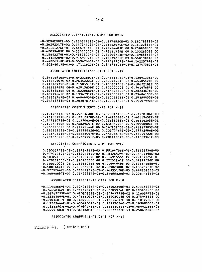
192

ASSOCIATED COEFFICIENTS C(P) FOR M = 14

-0 .32982902E-03 0 .85656967E-03-0 .12778550E-02 0 .18178172E-02 -0 .26292317E-02 0 .39724929E-02-0 .63862479E-02 0 .11102536E-01 -0 .21161276E-01 0 .44678380E-01-0 .10454403E CO 0 .25886806E 00 -0 .62039689E 00 O. ICOCOOOOE 01 0 .73131389E 00 0 .10326303E 00

0«15693270E-01-0 .41805724E-02 0 .28295718E-02-0 .18985544E-02 0 .13368289E-02-0 .97690924E-03 0 .73579225E-03-0 .56819804E-03 0 .448C6318E—03-0 .3596766CE-03 0 .29318707E-03-0 .24220744E-03 0 .20248013E-03-0 .17111623E-03 0 .14671107E-03-0 .12747082E-03

ASSOCIATED COEFFICIENTS C(P) FOR M=15

0 .24896510E-03-0 .64232601E-03 0 .9434764 5E-03-0 .13091306E-02 0 .182814G7E—02-0 .26362223E-02 0 .39915467E-02-0 .64405428E-02 0 .11240935E-01-0 .21503511E-01 0 .45536465E-01-0 .10672181E 00 0 .26383985E 00-0 .62913830E 00 O. IOOOOOOOE Cl 0 .74167684E 00 0•10757636E 00 0 .16220660E-01-0 .41444232E-02 0 .28283678E-02

-0 .18979641E—02 0 .13367912E-02-0 .97708599E-03 0 .73606153E-03 -0 .56851363E-03 0 .44840939E-03-0 .36005123E-03 0 .29359800E-03 -0 .24267733E-03 0 .20307014E-03-0 .17204140E-C3 0 .14907990E-03

ASSOCIATED COEFFICIENTS C C P » FOR M=16

-0 .19176313E-03 0 .49213680E-03-0 .71391613E-03 0 .971G0186E-03 -0 .13183191E-02 0 .18312978E-02-0 .26423833E-02 0 .40115632É-02 -0 .64938072E—02 0 .11370639E-01-0 .21816955E-01 0 .46314203E-01 -0 .10868540E 00 0 .26829651E 00-0 .63695772E 00 O. IOOOOOOOE 01

0 .75089002E 00 0 .11145144E 00 0 .16710270E-C1-0 .41115983E-02 0 .28281362E—02-0 .18978962E-02 0 .13370469E-02-0 .97742906E-03 0 .73642371E-03-0 .56888047E-03 0 .44878678E-03-0 .36045722E-03 0 .29406825E-03-0 .24 329551E-03 0 .20411812E-03-0 .17563941E-03

ASSOCIATED COEFFICIENTS C(P> FOR M=17

0 .15032978E-03-0 .38414763E-03 0 .55164 736E-03-0 .73 823334E-03 0 .9797C950E-03-0 .13204841E-02 0 .18328529E-02-0 .26491650E-02 0 .40322190E-02-0 .65452459E-02 0 .114915 55E-01-0 .22104185E-01 0 .4 7021250E—01-0 .11046356E 00 0 .27231261E OOrO.64399550E 00 O. IOOOOOOOE 01 0 .75913026E 00 0 .11494940E 00 0 .17164965E-01

-0 .40816608E-02 0 .28286461E-02-0 .18982388E-02 0 .13375463E-02 -0 .97792642E-03 0 .73689167E-03-0 .56933170E-03 0 .44925183E-03 -0 .36098857E-03 0 .29477984E-03-0 .24455820E-03 0 .20874678E-03

ASSOCIATED COEFFICIENTS C(P) FCR M=18

-0 .11968669E—03 0 .30476336E-03-0 .43402390E-03 0 .57315382E-03 -0 .74658362E-03 0 .98182921E-03-0 .13205926E-02 0 .18345028E-02 -0 .26567233E-02 0 .4C530329E-02-0 .65943798E-02 0 .11603976E-01 -0 .22367699E-01 0 .47666000E-01-0 .11208015E 00 0 .27594882E 00 -0 .65036017E 00 O. IOOOOOOOE 01 0 .76654612E 00 0 .11812282E 00

0 .17587664E—01-0 .40542011E-02 0 .28297054E-02-0 .18989003E-02 0 .13382503E-02-0 .97857 341E-03 0 .737489 31E-03-0 .56992256E-03 0 .4499100DE-03-0 .36186831E-03 0 .29637138E-03-0 .25063484E-03

ASSOCIATED COEFFICIENTS C1P) FOR M=19

Figure 43. (Continued)

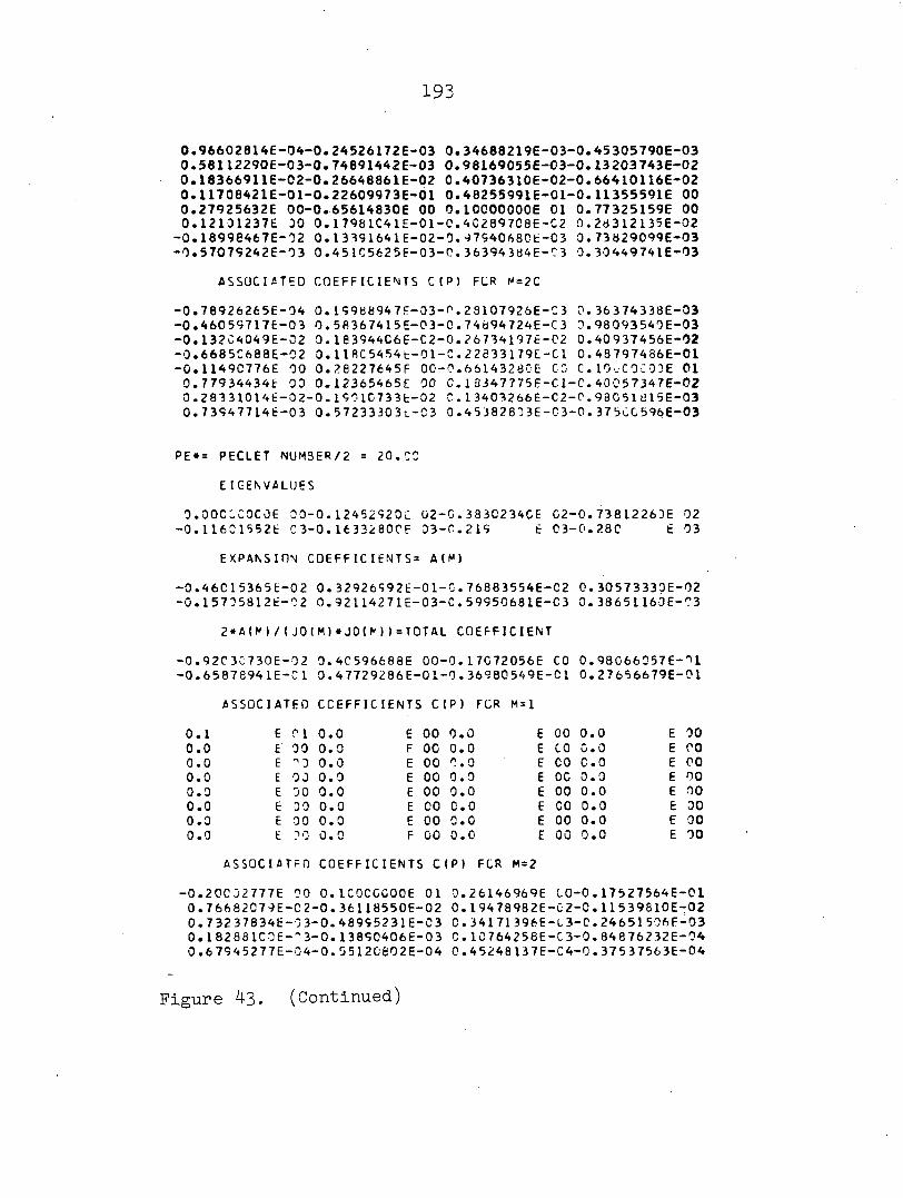
193

0 .96602814E-0 .58112290E-0 .18366911E-0 .11708421E-0 .27925632E 0 .12131237E

-0 .18996467E--0 .57079242E-

04-0 .24526172E-03 -0 . 74891442E-02 -0 .26648861E-01-0 .22609973E-00-0 .65614830E 30 0 . 17981C41E-02 0 . 13391641E-03 0 .45 1C5625E-

03 0 .34688219E 03 0 .98169055E 02 0 .40736310E 01 0 .48255991E 00 O. IOOOOOOOE 01 -C .4C289708E 02 -0 . 7940 iS8CE 03 -0 .36394384E

-03 -0 .45305790E-03 -03 -0 .13203743E-02 -02 -0 .66410116E-02 -01 -0 .11355591E 00 01 0 .77325159E 00

-C2 0 .28312135E-02 -03 0 .73829099E-03 -C3 0 .30449741E-03

ASSOCIATED COEFFICIENTS C(P) FCR M = 2C

-0 .78926265E-04 -0 .46059717E-03 -0 .132C4049E-02 -0 .6685C688E-02 -0 .1149C776E 00 0 . 7 79 34434E 00 0 .28331014E-02-0 .73S47714É-03

0 . 19988947F-03-0 .5B367415E-03-0 .163S44C6E-C2-3 . l lRC5454b-01 -0 .28227645F 00 -0 . 12365465E 00 0 . 19010733E-02 0 .57233303 t -C3

0 .23107926E 0 .74894724E 0 .26734197E C .22633179E 0 .6614328OE 0 .13347775E 0 . 1 3403266E 0 .45382803E

-C3 0 .36374338E -03 -C3 0.98093540E-03 -02 0.40937456E-02 -Cl 0.48797486E-01

CC C. lOvCOCOOE 01 -C1 —C.40 05 7347E-02 -C2-0.98C51Û15E-03 -03-0. 37 5GG 596E-03

PE* = PECLET NUM3ER/2 = 20 .CO

EIGENVALUES

0 . OOCCCOCOE 00 - 0 .12452S20C 02 -0 .3830234CE 02 -0 . 738 12263E 02 0 . 116C1552E 03 -•0 . 1633280CF 33 -0 .219 t 0 3 -•0 . 280 t 03

E XPANSI ON COEFFICIENTS 3 A(M)

•0 . 4 60 1 536 5 fc -0 2 0 .32926992É-01-0 .76883554E-02 0 . 30573330E- 02 •0 . 15705812 t -0 2 0 .92114271E-03-C .59950681E-C3 0 . 38651 160E- 03

2*A(M / ( J 0 ( M)«J0 (M)=T0TAL COEFFICIENT

•0 . 9203C730E-02 0 .40596688E 00 - 0 .17C72056E CO 0 . 98066057 E-•01 •0 . 65878941E-C1 0 .47729286E-01-•0 . 36980 549E-•01 0 . 276566 79E-•01

ASSOCIATED CCEFFICIENTS C(P) FCR M = 1

0 . 1 E 01 0 .0 E 00 0 .0 E 00 0 . 0 E 00 0 . 0 E 00 0 .0 F 00 0 .0 E CO 0 . 0 E 00 0 . 0 E r>3 0 . 0 E 00 0 .0 E CO 0 . 0 E 00 0 . 0 E 00 0 .0 E 00 0 .0 E 00 0 . 0 E 00 0 . 0 E 00 0 .0 E 00 o .o E 00 0 . 0 E 00 0 . 0 E 00 0 .0 E 00 0 .0 E 00 0 . 0 E 00 0 . 0 E 00 0 .0 E 00 0 .0 E 00 0 . 0 E 00 0 . 0 E 0 0 0 .0 F 00 0 .0 E 00 0 . 0 E 00

ASSOCIATED COEFFICIENTS CI IP ) FCR M=2

- 0 . •20C02777E 00 0 . ICOCCCOOE 01 0 .26146969E CO-- 0 . , 17527564E--01 0 . , 7 66 8207- JE-0 2-- 0 .3É118550E-02 0 .19478982E--0 2 ' - 0 . , 11539810E--02 0 .7 32 3 7834E-0 3 -0 .489S52 31E-0 3 C .34171396E-C3-0 .24651506F-03 0 .18288 ICO6-"3 -0 . 13890406E-03 0 . 10764258E-C3-0 .84876232E-04 0 .6 7945277E-04-0 .5 512C802E-04 0 .45248137E-C4-0 .37537563E-04

Figure 43. (Continued)

194

0 .314 3739 5E-04 -0 .26 554923E-04 0 . 226C5695E-04-0 . 19 3 t iC '654E-04 0 .16723889E-34-0 .14517660E-04 0 .126 72004E-C4-0 .11 1174 59E-04 0 .97998564E-05-0 .86766C67E-05 C .7714103 5E-0 5 -C .638 708 77E-05

ASSOCIATED COEFFICIENTS C(P) FCR M=3

0 .12161527E 00 -0 .428CG353S 00 C .1CC00C0CE 01 0 .48597379E 00 0 .323 5404AE-C 2 0 .10846275E-01-0 .56347597E-C2 0 . 33 12068JE-C2

-0 .20887932E-02 0v139C9732E-02-C .96688411E-03 0 .69578886E-03 -0 .51521193E-03 0 .39075134E-03-0 .3C246274E-C3 0 .2382 7311E-03 - 0 . 19060Û48E-03 0 . 15453C08E-03-0 . 12678728E-C3 0 . 105 13665E-03 -0 .88018923E-04 0 .74 325568E-04-0 .63254942E-C4 0 .542 18128E-04 -0 .46776380E-04 0 .4C598637E-04-0 .354 32127E-04 0 .31081819E-04 -0 .27395813E-04 0 . 24255043E-04-0 .2156678IE-04 0 . 19270998E-04

ASSOCIATED COEFFICIENTS CIP) FCR M=4

- 0 .83225631E-11 0 .26425649E 00 -0 .5728C658E 00 O. IOCCOCOOE 31 0 .69732095E 00 0 . 5 1228332E-01 0 .14182838E-C1-0 .67581390E-C2 0 .42223414E-02-0 .278C1992E-02 0 .19158558E-02-0 .13695406E-02 0 .10088897E-Û2-0 .762C7551E-03 0 .58798392E-03-0 .46199C05E-03 0 .36876567E-03-0 .29844723E-03 0 .244 50 256E-03-0 .20249532E-03 0 .16934414E-0 3 -0 . 14286689E-03 0 . 12149023E-C3-0 .104C6159E-03 0 .8 97 24341E-04-0 .77833443E-04 0 .67897393E-04-0 .59537681E-04 0 .52460199E-14-0 .46435489E-04 0 .41288201E-04-0 .36931034E-04

ASSOCIATED COEFFICIENTS CIP) FOR M=5

0 .57459048E-01-0 . 1 7409822E 00 0 .35509230E 00 -0 .70353641E 00 O. IOOOOOOOE 01 0 .89929286E 00 0 .11799907E 00 0 .2D2C1106E-01

-0 .73034300E-02 0 .48343247E-02-0 .32767127E-02 0 .23127457E-02 -0 .16867716E-02 0 .1264C7C6E-02-0 .96912663E-C3 0 .75754438E-03 -0 .60212308E-03 0 .46 55 9392E-0 3 -0 .39664797E-G3 0 .32767936E-03 -0 .27344845E-03 0 .23027014E-03-0 .19550387E-03 0 .16722521E-03 -0 .14401058E-03 0 .12479242E-03-C .10876016E-03 0 .95291815E-04 -0 .83905943E-04 0 .74229336E-04-0 .65983335E-04 0 .59080511E-04

ASSOCIATED COEFFICIENTS CIP) FCR M=6

- 0 . 3945400 1E-0 I 0 . 11627989E 00 -0 . 22534 2 58E 00 G .450C9143E ' "0 - 0 .8 1129199E 00 0 . 1C0CCC00C 01 0 . 11564944E 01 0 . 22498530E r 0 0 .3 243C195E-01-0 .700 71328E-02 C .5170054 3E-C2-0 .358G8C75E-C2 0 .25767208E-02-0 .19098799E-02 0 .14511690E-C2-0 .11260177E-C2 0 .8 89 5 540 1E-03 -0 . 71374891E-03 0 .58C51162E-C3-0 .47782450E-03 0 .3974 9932E-03-0 . 33383 143E-03 0 .2 82 76685E-03-0 .24 1372 84E-03 0 .20749343E-13-0 .17952113E-C3 0 .15624176E-C3-0 .13 6728C6E-H3 0 .12026608E-0 3 -0 .1063C682E-03 0 .94451945E-C4-0 .84669215E-04

ASSOCIATED COEFFICIENTS CIP) FCR M=7

0 .59459766E-02-0 . 1769C413E-01 0 .35869963E-01-0 .801204 26E-01 0 . 199061921 00 -0 .51064649E 00 O . ICCOOCGOE C l 0 .59687635E 10 0 .5 190C 169E-01 0 . 1C972098F-01-0 .46 122372E-C2 0 . 29 141953E-02

-0 .19366069 t -02 0 . 1 35C6503E-02-1 .978484?6E-C3 0 .73 I9C46 lE- n 3 -0 . 55986425E-03 0 . 43794683E-03-0 .34872998E-03 0 .28196533E-03 -0 . 2 3102987E-03 0 . 19151302E-03-0 . I6G39972E-03 0 . 13558099E-03 - 0 . I l555 l6bE-"3 0 .99 216C42F-04-C .85 772 536E-C4 0 . 74610669E-04 -0 .6527476 ÎE-C4 0 . 5741 7C8CO04-C . 507832 11E-C4 0 .453024 40E-14

Figure 43. (Continued)

LT\ CT\

CM m en m > r CM <M en O c c O O r r- o c V o O o O o UJ LU UJ LU Ui

1 Ui

1 tu UJ LU

o cr m m sO O C O r - cr O m o o cr iT\ r- o cr NO CM r »

iA o (M CM r- m r- o cr o in o r- m >* O r- >1- o m o r- o X <-o O o CXJ o m cr m m o C T m *• 4 - C O in o o r— NO h -o m r - m > c 00 m in <M m CO O r -m * cr m 00 m CO m rn (M

o o o o O o o o o O o O o O H o (M m m en -5" CM

1 m CM en o

o o C) o Y O u O O u o o o O

LU LU UJ LU Ui UJ LU UJ U4 UJ LU LU LU LU 03 in r- m O CD o O rn LU cr II o v0 r» N >o r*- T) o o 00 (M -r 51 o cr (X «J* O m O C > o >0 U >0 m

m o r- co m (X CO in o (D o a CM «O o h- m sT NÛ c o m LL CM CD O i a > r rsj m CM 4 ) r- u cr UL <M ir LL X m m NT cr O <7* m cr UJ O o

m •—« >r m >î* r- in Q m U

Û. o o o CJ o o o o o o 2 L o o O O 1 I 1 i I i 1 i

u CM o (M en m m <" <M en < m < O O o o O o o o o O O o o o h* O O

1 1 1 i i i 1 O II 1 i O 1 LL LU J_, LU •JJ UJ LU LO LU LU UJ

z r- o m e*> c m CM r» o O r- O II r- CJ UJ CT CD m >r cr m >j" o O Z cr m o

O kO cr cr o r- o O LU >r *4- u u m 30 in uo o cr r» o m cr m s: r- m

r- >J- cr m r- V c II CM w m >r cr r-U_ m CM rn m 00 sC o o m m rn o CD

C D CM cr o m r- CM <M <M U- CM cr -) cr cr CM >o m CM sO rsj LL m cr A m m

o o c UJ u

0

c

0

0 o o o o LU O O O O O X o O

1 * 1 1 1 CQ uo 1 u o CM o CM m m m •4" 21 LU O m rvj (M c CM LU O C» o o c.» o c O Z > 3 O o z O o O o t — 1 1 1 f 1 1 1

LU Z _J o 1 l 1 1 <1 UJ LU JJ UJ a i LU

1 LU < UJ UJ UJ UJ "s, LU LU

m «6 (M cr xO en sf < o > I/) m (M cr u m r - U > r m r - a u <M LU Z z >r m 2. CO m o m rn ir\ (T _J LU m cr O <M co m c r < O U O a 00 en < O m V*) <n cr m p- 50 cr LU X CM r- * in < CM f- O CD m sO G0 Q. h» UJ >r ao (M 00 cr

>r CM eu m GO m h- c r r- oo 4 -m m O K l h - CM «—4 r- I l o CM m M

* O o O o O O o O UJ O O o O O 1 1 a 1 » f 1

v

o o o o o o o o CM m >1- sT -4* m o CM m m o o o c o o o o o c c- o O o O O o O o

i o 1

UJ Ui UJ UJ LU UJ UJ LU UJ LU UJ UJ UJ UJ LU UJ UJ UJ UJ UJ <T o cr O <" O o >r o CM co m CM <- in (M co cr o r >r m ao CM m CM m >r m 00 cr O h- o o cr r- o r- m -T cr >4" o CD r-m cr >J- r- 00 O >r (M fs. 00 O C5 r- m h- 00 O H m sO 00 r-

o o o o o o o o (M 00 m CM r- m rn r-(M

o o o o o o o o o o o o O O o o o o o O

o o o o o o o o o CM m m m H CM CM m o o o o u o D o o o o o o O o o O o <_> O

LU LU LU UJ LU UJ UJ UJ LU LU UJ LU UJ UJ UJ UJ LU UJ LU CM cr o r- ff\ >0 o h- m m in m (M II rvj N* cr CM m o u r» CM m

21 X. r- 00 r- 00 cr sf ao cr z: o 4-o m r- cr cr o CM CM cr

ce oc 4- r- o CM 00 p- O cr ar cr o NÎ" o CJ o m m r- (_» cr m LL LL N o m vO m m cr X CM u>

o o o o o o o o CM CM CM r- O m

a o o o o o o o o CL o o o O o O c o a O o o O

o o o o o o o u o u f-4 CM m m 4" >r in o O r—4 CM m o. o o o o o o o o o o o o O o O o O o o

uo v o i i 1 1 1 1 IZ) 1 i i t - LU UJ UJ LU LU LU LU UJ LU LU UJ LU •— LU LU w LU z z cr O <- m z 00 m CO LU LU <r cr CO rvj CM CO r\j UJ o r- r» cr

cr O O m n CM o o in cr r- o en m r- o >r NT O CM

o cr m cr sT o NT CNJ LL m rn cr >r O r- LL sO cr c m LL r» o - T o r— in cr L L r- m

UJ o o o o o o o o LU m in tn CM «—< CD UJ -f o c O O o o o o o o o o o o o o O o O O o U O o o O

o o o o o o o o o o (M m m NÎ* •4- N* Q o H (M m U-. o o o o o o o o LL o o o o O O c O o C O o

h- t l # 1 1 » 1 •— 1 1 l < LU LU UJ UJ LU UJ UJ <1 • LU •JJ UJ LU <. LU LU UJ •XI

cr •n rn >1" m rr m r- p- rn u o cr V m r- m m W r» CM in >r o m o o o m m •4* O c r œ cr cr

«•) vo au m CM O o o (Z? uo m >0 o o IT «-I cr en vo c r > r cr o < < m o o cr CM m CN < cr m m

o 00 m CO O CM r- o > r m 00 o o o o o o o rxj r— h - —• r- m •—* CM m

0

0

o o o o o o o o O o o O o o o o o O

T) (D 2 G

*r4 -p c o o

on

CL)

hO •H PH

196

-0 . 21676757E-03 0 . 17584928E-03 -0 . 14435087E -C 3 -0 . 11975154E-03 - 0 . 10029067E-13 0 . 84714605 E- 04 -0 . 72116132E -04 3 . 61828C65E- 34 - 0 . 53352969E-34 0 . 46315248E-04 -0 . 40427951E -C4 0 . 35469558E- 04 - 0 . 31267484E-04 0 . 2 7686426 E-04 -•c . 24621165E -04 0 . 22C05151E- 04

ASSOCIATED CO EFF IC IENTS C tP ) FCR M=4

- 0 . 130 53761 £ 30 0 . 38669787E co­•0 . 73946473E CO 0 . 1 E 91 0 . 89529987E CO 0 . 91626573E-o l c . 19823 528E -C l -0 . 86451011E-02 0 . 55326554E-•02 - 0 . 369C0297E-02 0 . 2 5665 535E -C 2 -0 . 18474243E- 32 0 . 13681590E-•02 -•0 . 10 377546E- 02 0 . 80334676E -C3-•0 . 63290757E- 03 0 . 50631567E-•03 -•0 . 41052662E-03 0 . 33684745E -03 - 0 . 27934396E- 03 0 . 2 33 87690E- 0 3 -•0 . 1975C345E-03 0 . 16809539E -C 3 -•0 . 14408866E- 03 0 . 1 24 3 186 1E-•0 3 -•0 . 1C790623E- 03 0 . 9418048CE -04 - 0 . 82623796E- 04

- 0 . 72833569É- 04-•0 . 64495659E- 04 0 . 5 73 71 326E -C4- 0 . 51 3 55082E- 04

ASSOCIATED COEFFICIENTS C tP ) FOR M=5

0 .212 54638E-01-0 .69550440E-01 0 .16S23502E O. IOOOOOOOE 01 0 .51493C48E OC 0 .25263356E-

-0 .4 83 76664E-0 2 0 .29 7C755 4E-02 -0 .19425034E--0 .95504170E-0 3 0 .7049 3069E-03-0 .5 3401851E--0 .32603850E-03 0 .261234 7 3E-03 -0 .2 1222480E--0 .145C614 3E-0 3 0 . 1217421CE-03-0 .1C305 761E--0 .7 554 7460E-04 0 .65334721E-04-0 .5 6839 513E--0 .4 3715989E-04 0 .38621304E-04-0 .34282711E-

00-0 .447C4145E 00 01 0 .97914331E-02 02 0 .13354964E-02 03 0 .41343237E-03 03 0 .17451656E-03 C3 0 .87924432E-03 04 0 .49720880E-04

•04 0 .30628C44E-0*

ASSOCIATED COEFFICIENTS C tP ) FCR M=6

- 0 .10936200E-01 -0 .48185526E 00 0 . 10311699E-01-0 .13499398E-02-0 .4298569 OE-O 3 -0 .18525854E-03-0 .94838160E-C4-0 .54319437E-04-

0 .33936026E-01-0 . 0 . ICOOOOOOE 01 0 . 0 .47222403E-02 0 . 0 .9 7 312146E-03 0 . 0 .34094758E-03 0 . 0 .15466502E-03 0 . 0 .81768008E-04 0 . 0 .47900558E-04 0 .

75209671E-56032 993E 29462395E 72353305E 2 746475 IE 13033536E 70944623E 42455348E

•01 0 .18495116E 00 00 0 .39515829E-01

-02 -0 .19461118E-02 -03 -0 .55180018E-03 -03 -0 .22423854E-03 -03 -0 .11075826E-03 -04 -0 .61911462E-04 -04 -0 .37910586E-04

ASSOCIATED COEFFICIENTS C tP ) FOR M=7

0 . 5 94 5S766E-02-Û.17690413E-01 0 .3 586996 3E-0 .199C6192Ê 00 -0 .51064649E 00 O. IOOOOOOOE 0 .51900169E-01 0 . 1C972098E-01-0 . 46122372E-

-0 .19366069E-02 0 .135C6503E-02-0 .97848428E -0 .5 59 8642 5E-03 0 .437946 83E-03-0 .34 972998E -0 .23102987E-03 0 . 19151302E-03-0 . 16039972E -0 .11555168E-03 0 .99218042E-04-0 .85772536E -0 .65274763E-04 0 .5 7417C80E-04-0 .5078321IE

-01 -0 .8Û120426E-01 C l 0 .59687635E 00

•02 0 .29141950E-02 -03 0 .73090461E-03 -03 0 .28196533E-03 -03 0 .13558099E-03 -04 0 .74610669E-04 -04 0 .45302440E-04

ASSOCIATED COEFFICIENTS C tP ) FOR M=8

- 0 .34257335E-02 -0 .84793576E-01 0 .626 87302E 00 0 .28873749E-02-0 .73381556E-03-0 .2861S973E-03-

0 .984 7 5397E-02-0 .18524005E 0 . 21148686E 00 -0 .53463967E 0 .62 59 55 33E-01 0 .11700275E 0 . 19258943E-02 0 .13477436E 0 .56370996E-03 0 .44218024E 0 .235C9C15E-03 0 .19535368E

-01 0 .37375517E-C1 00 O. IOOOOOOOE 01

-01 -0 .45187239E-02 -02 -0 .97945201E-C3 -03 -0 .35304793E-03 -03 -0 .16400194E-03

Figure 43. (Continued)

197

0 .13894184E-03-0 .118677 5 2E-03 C .1G212076E-C3-0 .88467555E-04 0 .77116526E-04-0 .67616C4 7E-04 0 .59641081E-C4-0 .53124776E-04

PE»= PECLET NUMBER/2 = 50 .00

EIGENVALUES

0 .0 E 00 -0 .12774500E 02 -0 .41260625E 02 -0 .83860C00E 02 -0 .144 E C3-0 .221 E 03 -0 .308 E C3-0 .414 E 03

EXPANSION COEFFICIENTS: A t f )

-0 .33281711E-32 0 .32503302E-01-0 .74478236E-02 0 .34148875E-02 -0 .17873935E-32 0 . 9 934345 6E-03 -0 .599 506 81E-03 0 . 3865116CE-03

2*A(V) / ( JO(M)»JOm) =TOTAL COEFFICIENT

0 . 66563422E -02 0 .4C074308E 00 -0 .16537954E CO 0 . 10953486E : o •0 . 74973259b -3 1 0 .5147511CE- Ol -C .3698C549E--CI 0 .27656679E -01

ASSOCIATED COEFF ICIENTS C(P) FOR

H

II x:

0 . 1 E 01 0 .0 E 00 0 .0 E CO 0 .0 E 00 0 . 0 E 00 0 .0 E 00 0 .0 E 00 0 .0 E CO 0 . 0 E 00 0 .0 E 00 0 .0 E 00 0 .0 E CO 0 . 0 E 30 0 .0 E 00 0 .0 E 00 C .O E CO 0 . 0 t 00 0 . 0 E 00 0 .0 E 00 0 .0 E CO 0 . 0 E 00 0 .0 E 00 0 .0 E 00 0 .0 E CO 0 . 0 E 00 0 .0 E 00 0 .0 E 00 0 .0 E 00 0 . 0 £ 00 0 .0 E 00 0 .0 E 00 0 .0 E 00

ASSOCIATED COEFFICIENTS C(P) FOR M=2

-0 .20479462E CO 0 .78409053E-0 2 -0 .75292803E-0 3 -0 . 1882C540E-0 3 -0 .69949359E-04-0 .3237C303E-04-0 .17221831E-04-0 .10092239E-04-

0 .1 E 01 0 .37028484E-02 0 .5C389274E-03 0 .14296587E-03 0 .56749756E-04 0 .27343740E-04 0 .14950171E-04 0 .89355846 E-05

0 .2 7C15024E CO 0 , 0 .19997645E-02-0 , 0 .35153403E-03-0 0 .11080129E-C3-0 0 .46587488E-04-0 0 .23277793E-04-0 0 .13049732E-04-0 0 .79444526E-04-0

, 17571721E-01 11857057E-02

•25365180E-O3 , 87373922E-04 , 38650201E-04 , 19957309E-04 , 11449008E-04 . 70928859E-05

ASSOCIATED COEFFICIENTS C(P) FOR M=3

0 .13884795E 00 -0 .10509961E-01

-0 .23021613E-02 -0 .57333623E-03 0 .212Ô2876E-03

-0 .98441600E-04 -0 .52361477E-04 -0 .30683585E-C4

0 .46941214E 00 0 .11801896E-01 0 .15386455E-02 0 .43533430E-03 0 .17263917E-03 0 .83148951E-04 0 .45453320E-04 0 .27168890E-04

0 .1 E 01 0 . 0 .61243488E-02 0 . C .10723155E-Û2 0 .

-0 .33728104E-03 0 . 0 .14170556E-03 0 . C .70780527E-04 0 . 0 .39674632E-04 0 . 0 .24160456E-04 0 .

546266C7E 00 36309211E-02 77314742E-C3 26589923E-03 11754986E-03 60680910E-04 348C7878E-04 21592683E-04

ASSOCIATED COEFFICIENTS CIP) FOR M=4

Figure 43. (Continued)

198

-0 .12152316E Ou 0 .36375586E 00 -0 .70778879E 00 0 .1 E 01 0 .867751206 CO 0 .86659C24E-01 0 .18869892E-C1-0 .82857515E-02 0 .52890349E-02-0 . 35224897E-02 0 .24474007E-02-0 .17602224E-02 0 .13027536E-02-0 .98 764785E-03 0 .76424860E-C3-0 .60190481E-03 0 .481381946-0 3 -0 .39022021E-03 0 .32012328E-03-0 .26543076E-03 0 .22219653E-03-0 .18761657E-03 0 .15966 335E-C3-0 .13684787E-03 0 .118061436-0 3 -0 .10246748E-03 0 .89427571E-04-0 .78449356E-04 0 .69149924E-04-0 .61230469E-04 0 .54463 742E-04-0 .48 7475 51E-04

ASSOCIATED COEFFICIENTS C(P> FCR. M = 5

0 .212 54 638E-01-0 .6955044OE-01 C .16923502E 00 -0 .44704145E 00 0 .1OOCCOOOE 01 0 .51493048E 00 0 .25263356E-01 0 .97914331E-02

-0 .48376684E-02 0 .297C7554E-02-0 .19425034E-02 0 .13354964E-02 -0 .955041706-03 0 .7C4S3069E-03-0 .53401851E-03 0 .41343237E-03 -0 .32603850E-03 0 .261234 73E-03-0 .21222480E-03 C .17451656E-03 -0 .145C6143E-C3 0 . 12174210E-03-0 .10305761E-03 0 .87924432E-03 -0 .75547460E-04 0 .65334721E-04-0 .5 6839513E-04 0 .49720880E-04 -0 .4 3715989E-04 0 .38621304E-04-0 .34282711E-C4 0 .30628044E-04

ASSOCIATED COEFFICIENTS C(P) FCR M=6

- 0 .10936200E-01 0 .33936C26E-01-0 .7 5209 671E-01 0 .18495116E 00 -0 .48185526E 00 0 . ICOOOCOOE 01 0 .56032993E 00 0 .39515829E-01

0 . 1 0 3 1 1 6 9 9 E - : i -0 .47222< . 0 3 F - C 2 3 . 29462 395E-02-0 . 19461118E-02 3 . l 3 4 3 S 3 9 8 t - 3 2 - 0 . 97 i l2146E-03 ? .72 353305E-03-0 .55160018E - 0 3 0 . 4 2 9 8 3 6 9 3 E - C 3 - 0 . 34^ 9 4 758 E - C 3 C . 2 7464 75 1E-03 -0 . 22423854E-03 3 .185 2 5854E - C 3 -0 .15466502E - 3 3 0 . 13033536E-03-0 .11C75826E-03 3 . 94R3e i60E-04-0 .8176 t iC08E-04 0 .7C944623E-C4-0 .61911462E-34 0 .54319437 t -14 -0 .479CC558E-34 C .42455348E-04-0 .37910586E-04

A S S O C I A T E D C O E F F I C I E N T S C ( P ) F C R M=7

3 .5 94 5 9 766É - 3 2 -0 .1769C413E-91 0 . 35869963E-01-0 .80120426E-01 3 .199Û6192C 00 -0 .51064649E OC 0 . ÎÛCOCCOOE 01 0 .59687635E 30 0 .519CC169E-C1 0 .1C972C98E-01-C .46122372E-02 0 .29141950É-02

- 0 . 19366064E-^2 0 .135C6503E-02-0 .97E48428E-03 0 .73090461E-°3 -0 .55936425E - 33 0 .42794683E-03 -C .34672 998E-03 0 .28196533E-03 -0 .23132987E-03 0 . 19151$C2E-03-0 .16Û39972E-03 C . 13558G99E-03 -0 .11555163E - 33 0 .992 l8 !42E-04-3 .85772536E-04 0 .74610669E-04 -0 .65274 76 3E-C4 0 . 5741738CE-04-0 .507832 11E-C4 0 .45302440E-0*

A S S O C I A T E D C O E F F I C I E N T S C ( P ) F O R M = 8

-0 .34257335E-32 0 .99475397E-C2-3 .18524 00 5E-C1 0 .37375517E-01 -0 .84793576 t -C l 0 .21148686E CO-3 . 5 3463 96 7E OC 0 . ÎOOCOOOOE 01

0 .626573C2E 00 0 . 62595533E-C1 0 . 1 1700275E - 01 - 0 . 45187239E-02 0 .2 88 73749E-02-0 . 192 58943E-02 C . 13477436E-G2-0 .97945201E-03 0 .7 33 81556É-3 3 -0 .5637C^96E-C3 C .44 218024E-33-0 .35304 793E-03 0 .2 86 19973E-03-0 . 2 35C9v . 15E-03 C . 19535368E-03-0 .16400194E-03 0 . 13894 184E-03-0 . 1 1867752E-03 C .1C212076E-03-0 .88467555E-04 0 .77116526E-04-0 .67616C47E-04 0 .59641081E-04-0 .53124776E-04

P E » = P E C L E T N U M B E R Z 2 = 5 C C . 0 0

Figure 4-3. (Continued)

199

EIGENVALUES

0 .0 E CO- 'O . 12825C0CE 02 -0 .41925000E 02 -0 .87 E 02 -0 .1482 E 03 -0 .2252 E 03 -0 .3185 E 03 -0 .4275 E 03

EXPANSION COEFFICIENTS: A(M)

- 0 .28096343E-02 0 .3231C705E-01-0 .72578 505E-C2 0 .33499746E-02 -0 .17873935E-02 9 .99343456E-03-C .59950681E-03 0 .38651160E-03

2»A(P) / I J0 (M)»J0 (M))=T0TAL COEFFICIENT

-0 .56192686E-02 0 .39836850E 00 -0 .16116118E CO 0 .10745273E 00 -0 .74973259E-01 0 .51475110E-01-C .36980549E CO 0 .27656679E-01

ASSOCIATED COEFFICIENTS C(P) FCR M=1

0 . 1 E 01 0 .0 E 00 0 .0 E 00 0 .0 E 00 0 .0 E 00 0 .3 E 00 c . o E 00 0 .0 E 00 0 .0 E 00 0 .0 E 00 0 .0 E CO 0 .0 E CO 0 .0 E CO 0 .0 E 00 c . o E CO 0 .0 E 00 0 .0 E 00 0 .0 E 00 c . o E CO 0 .0 E CO 0 . 0 E 00 0 .0 E 00 0 .0 E CO 0 .0 E 00 0 .0 E 0 0 0 .0 E 00 0 .0 E CO 0 .0 E "0 0 .0 E 00 0 .0 E 00 c.o E CO 0 .0 E 00

ASSOCIATED COEFFICIENTS C(P) FCR M=2

-0 .20575475E 00 0 .1 E 01 0 .78746346E-C2-0 .37206428E-02 0 .7 56S5492È-0 3 -0 .5C662 526E-C3 0 .18924956É-03-0 .14 3762 53E-03 0 .70342484E-"4 -0 .57069299E-04 0 .32553355E-04-0 .27498^06E-04 0 .17319 529E-04-0 .15C35C34E-04 3 .101496C9É-04-0 .89 864CC6E-05

0 .27182292E CO-O.17579138E-01 0 .20099174E-02-0 . i l 919197E-02 C .3 5345 930E-03-0 .25 5C512 5E-03 0 .11142085E-03-0 .87863637E-04 C .46d5C242E-04-0 .38868491E-C4 0 .23409659E-04-G.20070453E-04 0 . I 3123847E-04-0 .11514063E-34 C .79896 517E-C5-0 .71332674E-05

ASSOCIATED COEFFICIENTS CIP) FOR M=3

0 . 14297777k 00 -0 .47915178E 00 C . l E C l 0 .56043385E CO 0 .1236C694E-01 0 .120 32 792E-01-C .62380849E-02 0 .37053676E-02 0 .23521254E-02 0 .15732978E-02-C .1C97C934E-02 0 .79134856E-03

-0 .587C2378E-03 0 .445R4C51E-03-0 .34549056E-03 0 .27241587E-C3 -0 .21807414E-03 0 .176913 86E-03-C .14522799E-03 0 .12048144E-03 -0 .10G9C355E-03 0 .8 5233474E-04-0 .72558708E-C4 0 .622C8160E-C4 -0 .53681462E-04 0 .46600796E-04-0 .406775GCE-04 0 .35688741E-04 -0 .31460891E-04 0 .27857840E-04-0 .24 77375 2E-C4 0 .22141748E-04

ASSOCIATED COEFFICIENTS CIP) FCR M=4

-0 .13375234E 00 0 .39483479E 00 -3 .75C96467É CO 0 .1 E 01 0 .9C29 1600E 00 0 .927C4155E-01 C .2C12302 5E-01 -C .87748476E-02 0 .56187997E-02-0 .37488439E-02 0 .26C81887E-02-0 .18778005E-02 0 .13908935E-02-0 .10551437E-02 0 .81689928E-03-0 .64 364402E-03 0 .514 94409E-0 3 -0 .4 7 754S44E-03 0 .34262865E-C3-0 .28415160E-03 0 .23791165E-03-0 .20091778E-03 0 .17100651E-03-0 .146588C4E-03 0 .126478C8E-03-0 .10978295E-03 0 .95620316E-C4-0 .84063870E-04 0 .74104 187E-C4-0 .65 62 1825E-04 0 .56 37405 0E-04 -0 .522 54208E-04

Figure 43. (Continued)

200

ASSOCIATED COEFFICIENTS C(P) FCR M=5

0 .21254638E-01-0 .69550440E-01 0 .16S23502E 00 -0 .447C4145E 00 0 . ICODCOOOfc 31 0 .51493C48E 00 0 .25263356E-C1 0 .97914331E-02

-0 .48376684E-02 0 .29 7C7554E-02-0 .19425034E-C2 0 .13354964E-02 -0 .95504170E-C3 0 .70493C69E-03-0 .53401851E-C3 0 .41343237E-33 -0 .32603850E-03 0 .261234 73E-03-0 .2 1222480E-03 0 .17451656E-03 -0 .145C6143E-03 0 . 121742 10E-03-C ,10305761E-C3 0 .87924432E-03 -0 .75547460E-04 0 .65334721E-04-0 .56839513E-04 0 ,497208H0E-04 -0 .43715989E-04 0 . 38621304E-04-C .34282711E-04 0 .30628044E-04

ASSOCIATED COEFFICIENTS C(P) FCR f=6

-0 .1C936200E-01 0 .33936C26E-01-0 .75209671E-01 0 .18495116E 00 -0 .4B1B5526E CO 0 .1C0CCC00E 01 0 .56032993E CO 0 .39515829E-01

0 .10311699L-C1-0 .47 222403E-02 C .29462395E-02-0 .19461118E-02 0 .134 99398E - 0 2-0 .97 312146E-03 0 .72 353305E-C3 - 0 . 55160C18E-03 0 .429B569OE-O3-0 .34094758E-03 0 .27464751E-03-0 .22423854E-03 0 .18525854E - 03-0 .15466502E-03 0 .130 33 536E-C3 - 0 .110758P6E-03 0 .948 3 816 0E-04 -0 .8176 8C08E-04 C .7094462 3E-04-0 .61911462E-04 0 .54319437E-04 - 0 . 479C0558E-04 0 .42455348E-04-0 .3791C586E-04

ASSOCIATED COEFFICIENTS C(P) .FOR M = 7

0 .594 59766E-0 2 -0 .17 69C413E-01 0 .35869963E-C1-0 .80120426E-01 0 .199C6192E 0 0 -0 .51064649E 00 0 . 10000000E 01 0 .59687635E 00 0 .51900 169E-01 0 .1C972098E-01-0 .46122372E-C2 0 .29141953E-02

-0 .19366069E- r 2 0 .135C6503E-02-0 .97848428E-03 0 .73C90461E-03 - 0 . 55986425E-03 0 . 43794683E-03r -0 . 34872998E-03 0 . 28 196533E-03 -0 .231Ù2987E-03 0 .19151302E-03-C .16339972E-C3 0 .13558C99E-03 -0 .11555168E-03 0 .99 218C42E-04-0 .85772536E-04 0 .74610669E-04 -0 .65274763E-04 0 .57417C80E-04-0 .50783211E-04 C .45302440E-04

ASSOCIATED COEFFICIENTS C(P) FOR M=8

- 0 .34257335E-02 3 .98475397E-02-0 .18524005E-01 0 .37375517E-01 -0 .84793576E-01 0 .21148686E 00 -0 .53463967E CO O. IOCOOOOOE 01

0 .6 26 87302E 00 0 .6259 5533E-01 C . 11700275E-01-0 .45187239E-02 0 .28873749E-C2-0 .19258943E-02 0 .13477436E-02-0 .9794520IE-03 0 .73381556E-33-0 .56370S96E-03 0 .44218024E-03-0 .35304793E-03 0 .2861S973E-03-0 .23509015E-03 0 . 19535368E-0 3 -0 .16400194E-03 0 .13894184E-03-0 .11867752E-03 0 .1C212076E-03-0 .88467555E-04 0 .77116526E-04-0 .67616047E-04 0 .5 9641081E-C4-0 .53124776E-04

EXPANSION COEFFICIENTS-APPROXIMATE SOLUTION =AIM>

-0 .12SOCOOOE 00 0 .52251210E 00 -0 . 15740605E 00 0 .83368063E-01 -0 .5 39 20340E-01 0 .38631859E-01-0 .29466385E-01 0 .23449953E-01 -0 .19244937E-01 0 .16167276E-01-0 .13833557E-01 0 .12013550E-01 -0 .10561404E-01 0 .93806066E-02-0 .84C49754E-02 0 .75877689E-02 -0 .68951182E-02 0 .63019386E-02-0 .57893025E-02 0 .53426601E-01 -0 .49506944E-02 0 .46044638E-02-0 .42968244E-02 0 .40220086E-02 -0 .37753057E-02 0 . 35528505E-02-0 .33514274E-02 0 .31683555E-02 -0 .300 13725E-02 0 .28485668E-02-0 .27C83062E-02 0 .25791977E-02

Figure 43. (Continued)

201

EXPANSION COEFFICIENTS = AIM) 0 .21567742E 00 -0 .616413C1E-C1 0 .3 1368 24 8E-C1-0 .19714130E-01 0 . 1 3833470 E-0 1 -0 . 1C 388364 E-01 C .816 84 35 5E-C2-0 . ' 66400466E-02 0 .55351745E-02-0 .47059839E-02 C .4C649476E-C2-0 .35 5 72843E-02 0 .31471403E-02-0 .281C1667E-02 C .25293093E-C2-0 .22923041E-02 0 .20901305E-02-0 .19 16C209E-02 0 .17648G89E-02-0 ;16324899E-92 0 .15159134E-02-0 .14125855E-02 0 .13204 821E-C2-0 .123 79699E-02 0 .11637065E-02-0 .1C965820E-02 C .1C356711E-C2-0 .98C1976CE-03 0 .92950521E-03-0 .883C3637E-03 0 .84031431E-0 3 -0 .80C92935E-03

TOTAL COEFFICIENTS = 2A l M ) / ( JC(M * JO m)

0 .160 19 74 5E 01 -0 .1C647993E 01 C .85139924E 00 -0 .72964524E 00 0 .64852365E CO-O.58954284E 00 0 .54418020E CO-O.50789363E 00 0 .478C1250E 00 -0 .45285C57E CO 0 .43128389E GO-0 .41253C71E 00 0 .39602820E 00 -0 .38135952E 00 C .3682C842E CO-O.35633015E 00 0 .34553179E CO-O.33565905E 00 0 .32658688E 00 -0 .31821258E 00 0 .31C451C7E 00 -0 .3C323109E 00 0 .29649246E 00 -0 .29018398E 00 0 .284S6174É 00 -0 .27868787E CO C .27342953E CO-O. 26845800E r -Q 0 .26374814E 00 -0 .25927777b 00 0 .25502726E OC-O.25G97916E DO

E IGENVALUES

PE« =0 .05

-0 .11899777E 00 -0 .27475672E 00 -0 •74529690E OO-O.9C230405E 00 -0 .1373424 5E 0 1 -0 .153C4807E 01 -0 . 200 16716E 0 1 -0 .2158 7397E 01 -0 .26299525E 0 1 -0 .2787C257E 01 -0 .32582517E 0 1 -0 .34153235E 01 -0 .38865512E 0 1 -0 .40436275E 01 -0 .4 5148585E 0 1 -0 .46 71935 7E 01

-0 .43143817E 00 -0 .58832800E 00 -C . 1C593325E C1-0 .12163742E 01 -0 .16U75413E G1-0 .18446C52E 01 -0 .23158C96E 01 -0 .24728607E 01 -0 .29440992E 01 -0 .31011735E 01 -C .35723992E 01 -0 .37294750E 01 —0.42CC7045E C1-0 .43577815E 01 -C .48290132E 01 -0 .49860910E 01

PE* =C .50

-0 .10838926E 0 1 -0 .26378680E 01 -0 .42C36687E C1-0 .57720915E 01 -0 .73415050E 01 -0 .89113965E 01 -0 .10481554E C2-0 .12051877E 02 -0 .13622307E 02 -0 . 15192812E 02 -C . 16763371E C2-0 . 18333971E 02 -0 .19904602E 02 -0 .21475256E 02 -0 .23C45930E C2-0 .24616620E 02 -0 .26187320E 02 -0 .27758C32E 02 -0 .29328755E C2-C .30899485E 02 -0 .3247C255E 02 -0 .34040962E 02 -0 .35611707E C2-0 .37182457E 02 -0 .38753212E 02 -0 .4C323967E 02 -0 .41894727E C2-0 .43465492E 02 - 0 .4 5C3625 7E 02 -0 .466C7C25E 02 -0 .48177792E C2-C .49748565E 02

PE* =1 .00

-0 .19562544E 01 -0 .5C426760E Ol -C .81681600E Cl -O .113G2130E 02 -0 .14439287E 02 -0 .17577S79E 02 -C .2 071752 t iE 02 -0 .23857604E C2 -0 .26998025E 02 -0 .3C138686E 02 -0 .33279 52 0E C2-0 .36420483E 02 -0 .39561545E 02 -0 .427C26E4E 02 -0 .45843884E C2-0 .48985135E 02 -0 .52126420E 02 -0 .5526775CE 02 -0 .58409100E C2-0 .61550480E 02 -0 .64691950E 02 -0 .67833295E 02 -0 .7C974725E C 2 -0 . 74 U6 170E 02 -0 .77257630E 02 -0 .8C399C95E 02 -0 .83540575E C2-0 .86682C60E 02 -0 .89823555E 02 -0 . 92965C50E 02 -0 . 96 1C656CE C '2 -0 . 99248C70E 02

PE* =5 .00

Figure 44. Model III. Constant wall temperature - plug flow - eigenvalues and coefficients

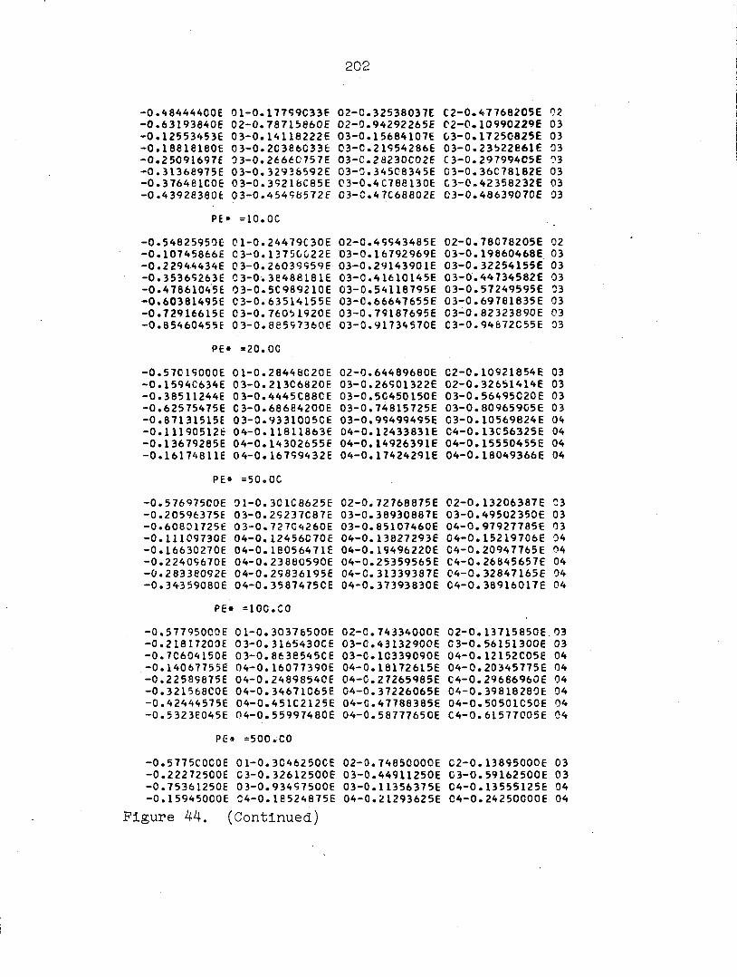
202

-0 .48444400E 01 -0 .63193840E 02 -0 .12553453E 0 3 - o . i e e i e i e o E 0 3 -0 .25091697E 03 -0 .31368975E 03 -0 .376481C0E 03 -0 .439263606 03

0 .17799G33E 0 .78715860E 0 .14118222E

-0 .2C386033E 0 .2666C757E

-0 .32936592E -0 .39216C85E -0 .454SB572£

02 -0 .32538037E 02 -0 .94292265E 03 -0 .15684107E 03 -C•21954286E 03 -C .28230C02E 03 -0 .345C834 5E 03 -0 .4C788130E 03 -C .47C68802E

C2-0 .47768205E 02 02 -0 .109902296 03 G3-0 .1725G825E 03 03 -0 .23b22661E 03 C3-0 .297994C5E 03 G3-0 .36C78182E 03 C3-0 .42358232E 03 C3-0 .4863907CE 03

PE* =10 .OC

-0 .54825950E 01 -0 .24479C30E -0 .10745866E 03 -0 .1375GÛ22E -0 .22944434E 0 3 -0 .26039S59E -0 .35369263E 0 3 -0 .36488181E -0 .47861045E 03 -0 .5C989210E -0 .60381495E 0 3 -0 .63514155E -0 .72916615E 03 -0 .760b1920E -0 .85460455E 0 3 -0 .885S7360E

02 -0 .49943485E 02 -0 .78078205E 02 03 -0 .16792969E 03 -0 .19860468E 03 03 -0 .2914390 IE 03 -0 .32254155E 03 03 -0 .41610145E 03 -0 .44734582E 03 03 -0 .54118795E 03 -0 .57249595E 03 03 -0 .66647655E 0 3 -0 .69781835E 03 03 -0 .79187695E 03 -0 .82323890E 03 03 -0 .91734570E C3-0 .94672C55E 03

PE* =20 .00

-0 .57019000E 01 -0 .28448C20E -0 .1594C634E 03 -0 .213C6820F -0 .38511244E 0 3 -0 .4445C880E -0 .62575475E C3-0 .68684200E -0 .87131515E 03 -0 .93310050E -0 .11190512E 04 -0 .11811863E -0 .13679285E 04 -0 .14302655F -0 .16174811E 0 4 -0 .16799432E

02 -0 .64489680E 02 -0 .10921854E 03 03 -0 .26901322E 02 -0 .32651414E 03 03 -0 .5C450150E 03 -0 .56495C20E 03 03 -0 .74815725E 03 -0 .809659G5E 03 03 -0 .99499495E 03 -0 .10569824E 04 04 -0 .12433831E C4-0 .13C56325E 04 04 -0 .14926391E 04 -0 .15550455E 04 04 -0 .17424291E 04 -0 .18049366E 04

PE* =50 .OC

-0 .57697500E 01 -0 .301C8625E -0 .20596375E 0 3 -0 .29237C87E -0 .60801725E 03 -0 .727G4260E -0 .11109730E 04 -0 .12456C70E -0 •166 30270E 04 -0 .18056471E -0 .22409670E 04 -0 .23880590E -0 .2833G092E 04 -0 .29836195E -0 .34359080E 04 -0 .35874750E

PE* =100 .CO

02 -0 .72768875E 02 -0 .13206387E 03 03 -0 .38930887E C3-0 .49502350E 03 03 -0 .85107460E 04 -0 .97927785E 03 04 -0 .13827293E 04 -0 .15219706E 04 04 -0 .19496220E C4-0 .20947765E 04 04 -0 .25359565E C4-0 .26845657E 04 04 -C .31339387E C4-0 .32847165E 04 04 -0 .37393830E 04 -0 .38916017E 04

-0 .577 95000E 01 -0 .30376500E 02 -0 .74334000E 02 -0 .13715850E 03 -0 .218 I7200E 03 -0 .3165430CE 03 -0 .43132900E 0 3 -0 .56151300E 03 -0 .7C604150E 0 3 -0 .8638545GE 03 -0 .10339090E 04 -0 .12152C05E 04

; -0 .14067755E 04 -0 .16077390E 04 -0 .18172615E 04 -0 .20345775E 04 -0 .22589875E 04 -0 .24898540E 04 -0 .27265985E C4-0 .29686960E 04 -0 .321568C0E 04 -0 .34671C65E 04 -0 .37226065E 04 -0 .39818280E 04 -0 .42444575E 04 -0 .451C2125E 04 -0 .47788385E 04 -0 .50501C50E 04 -0 .5 32 38045E 0 4 -0 .55997480E 04 -0 .5877765GE C4-0 .61577005E 04

PE* =500 .CO

-0 .5775C0C0E 01 -0 .3C46250CE 02 -0 .74850000E C2-0 . 13895000E 03 -0 .22272500E C3-0 .32612500E 03 -0 .44911250E 03 -0 .591625C0E 03 -0 .75361250E 03 -0 .93497500E 03 -0 .11356 375E C4-0 .13555125E 04 -0 .15945000E 04 -0 .18524875E 04 -0 .21293625E 04 -0 .24250000E 04

Figure 44. (Continued)

203

-0 .27392625E 04 -0 .30720375E 04 -0 .34231500E C4-0 .37924625E 04 -0 .417985C0E 04 -0 .4585C875E 04 -0 .50080500E 04 -0 .54485625E 04 -0 .59C64375E 04 -0 .63815125E 04 -0 .68735750E 04 -0 .738245C0E 04 -0 .790795COE 04-0 .844S850CE 04 -0 .90C79875E 04 -0 .95821500E 04

Figure 44. (Continued)

204

PE*= PECLET NUMBER/2 = C .C5

EIGENVALUES

-0 .1183C162E 00 -0 .27428855E 00 -0 .43100135E 00 -0 .58790090E 00 -0 .744874C0E 00 -0 .9018B330E 00 -0 .1C589130E 01 -0 .12159555E 01 -0 .13730062E 01 -0 .153C0628F 01 -0 .16871237E C1-0 .18441877E 01 -0 .20012542E 01 -0 .21583226E 01 -0 .23153925E C1-0 .24724637E 01 -0 .26295357E 01 -0 .27866C87E 01 -0 .29436822E 0 1 -0 .31007567E 01

EXPANSION COEFFICIENTS= A ( M)

0 . 21544662E 00 -0 .61688734E-Ol 0 .13842542E-01-0 .10 39422 7E-01 0 .55373272E-02-0 .47076225E-02 0 .314 79699E-02-0 .281C855 0E-02 0 .20905696E-02-0 . 1916426 : E -02

0 .31395491E-01-0 .19729164E-01 0 .81724856E-02-0 .66429402E-02 0 .40662291E-02-0 .35583051E-02 0 .25298865E-02-0 .22 928010E-02 0 .17652353E-02-0 .16332503E-02

2»A(M/ ( J1 (M)*J1 (M)=TOTAL COEFFICIENT

0 .15987776E 01 -0 .1C656185E 01 0 .85213864E 00 -0 .73020165E 00 0 . 64894891E 00 -0 .58987554E OC 0 .54445001E 00 -C .50811493E 00 0 .47819839E 00 -0 .453C0826E 00 0 .43141986E 00 -0 .412649C9E 00 0 .39613259E 00 -0 .38145293E 00 0 .36829245E CO-O.35640739E 00 0 .3456C439E 00 -0 . 33573C38E 00 0 .32666579E 00 -0 .31836080E 00

ASSOCIATED COEFFICIENTS C(P) FCR M=1

0 . lOOOCOOOE 0 1 0 . 2295 77 77E-02-0 .22134662E-03 0 .49714687E-04 -0 .16462380E-04 0 .68199206E-05-0 .32731006E-05 0 .17438139E-05 -0 .10045676E-05 0 .614948 35E-06-0 .39519141E-06 0 .26427657E-06 -0 .182694C4E-06 0 .1298 96 80E-06-0 .94612184E-07 0 .70369137E-07 -0 .53305915E-07 0 .410389 59E-07-0 .32053138E-07 0 .25359604E-07 -0 .20298079E-07 0 .16416614E-07-0 .13408160E-0 7 0 .11045774E-07 -0 .91728265E-08 0 .76 738536E-08-0 .64637191E-08 0 .54788840E-08 -0 .46714089E-08 0 .40047482E-08-0 .34507788E-C8 0 .29876704E-08

ASSOCIATED COEFFICIENTS CIP) FOR M=2

-0 .27528517E-02 O. ICOCOOOOE 01 0 .28882255E-02-0 .31861983E-03 0 .82239213E-04-0 .30 212942E-04 0 .13549904E-C4-0 .69208129E-05 0 .38764425E-05-0 .2 3 26 7281E^05 0 .14739 712E-05-0 .97 513163E-C6 0 .66853613E-06-0 .47223931E-06 0 .34216645E-06-0 .25340931E-06 0 .19128888E-06-0 .14683765E-06 0 .11440290E-06-0 .90322335E-07 0=7 216444 l f c -07 -0 .58261042&-07 0 .47530216E-07-0 .39109285E-07 0 .32443790E-07-0 .27116830E-07 0 .22821768E-07-0 .19330298E-07 0 .164 7C505E-07-0 .14111578E-07 0 .12153016E-07-0 .10516950E-07

ASSOCIATED COEFFICIENTS C(P) FCR M=3

0 .23905989E-03-0 .31370C1CE-02 0 . lOCOOOOOE 01 0 .30233459E-02 -0 .3527S313E-03 0 . 96 352634E-04-0 .37183375E-C4 0 . 17388604E-04 -0 .92029506E-05 0 .53137802E-05-0 .32740914E-C5 0 .21218623E-05 -0 .1432C126E-05 0 .99918265E-06-0 .71691150E-C6 0 .52674904E-06 -0 .39503768E-06 0 .30159885E-06-0 .23390920E-06 0 .18395944E-06

'Figure 45. Model IV. Constant wall temperature - fully-developed laminar flow - eigenvalues and coefficients

205

-0 . 14649019E- 06 0 . 11796892E-06 -C . 95968396E- C 7 0 . 787937516-07 - 0 . 652 3962 76 -07 0 .54435516E-07-0 . 45744414E-07 0 . 386939356-07 -0 . 32929665E-07 0 .28182823E-07 -0 . 24247523E-07 0 . 20964729E-07

ASSOCIATED COEFF ICIENTS C(P) FCR M=4

- 0 . 52183573E-04 0 .33876784E- OS-0 . 32199862E- 02 0 . lOOOOOOOE 01 0 . 30805789E- 02 -0 .36841333E-OS 0 . 10352883E-03 -0 . 41056925E-04 0 . 19683151E-04 -0 . 1C652193E- 04 0 . 62742553E-05 -0 . 39352584E-05 0 . 259 12955E-•05 - 0 .17740379E-05 0 . L2539175E- 05— 0 . 91026697E-06 0 . 6 75 96613 E— 06 -0 . 5 11 886 96E-06 0 . 3 9429840E- 06 -0 . 30831116E-06 0 . 244 3C456E- 06 - 0 .1959C458E-06 0 . 15878303E- 06 -0 . 12994811E-06 0 . 107 29042E- 06 - 0 .89299258E-07 0 . 74875705E- 07 -0 . 63210208E-07 0 . 53698572E- 07 -•0 . 45884779E- 07 c . 39421029E- 07 -0 . 34039804E-•07

ASSQCIATED COEFF ICIENTS 1 C IP ) FCR M=5

0 . 17041381E-•04 - 0 .858C5543E- 04 0 . 37232433E-•03 -•c . 32476223E-•02 0 . 100CC000E 01 0 .311C7986E- 02-•0 . 37682371E-•C3 0 . 10 764201E-•03

- 0 . 434070556--04 0 .21145330E- 04-•0 . 11615631E--04 0 . 69366551E-•05 - 0 . 44061300E-•05 0 . 29352243E- 05-•0 . 20310054E-•05 0 . 14496537E-•05 - 0 . 106 18719E-•05 0 .79511929E- 06-•0 . 60675 382E-•C6 0 . 47070508E-•06 - 0 . 37048987E--06 0 . 29538512E- 06-•0 . 2 38 22424E-•06 0 . 194119356-•06 - 0 . 15966520E--06 0 . 13244709E- 06-•0 . 11C72531E--06 0 . 93228041E-•07 - 0 . ,790125696--0 7 0 .67372224E- 07-•0 . 57771 037E-•C7 0 . 497989486-•07

ASSOCIATED COEFF ICIENTS C tP ) FCR M=6

- 0 . , 70043122 E--05 0 .31200752E- 04-- c . 10011857E--C3 0 . , 38 714901E-•03 - 0 . , 325899236--02 0 . lCOOOOOOE 01 0 . 3 1290 111E--02 --0 . , 381870656-•03

0 . , 110210966--0 3 --0 .44933653E-•04 0 . , 22129 13 1E--04 -•0 . , 122843796--04 0 . , 74C93378E--05 --0 .47505288E-•05 0 . , 31924001E--05 --0 . , 222702016-•05 0 . . 16016766E--05 --0 .11815657E-•05 0 . 1 8906107 7E--06 --0 .683831946-•06 0 . , 53357088E--06 --0 .42225355E--06 0 . , 338367176--06 --0 . . 274193406--06 0 , . 22443435E--06 --0 .18538204E--06 0 . , 15439509E--06 --0 . . 12 956179E--06 0 . . 10947813E--06 --0 .93099456E--07 0 . , 796394336--07 --0 . •68500412E--07

ASSOCIATED COEFFICIENTS C(P] 1 FCR M= 7

0 , . 33449229E--05 --0 .139C6666E--04 0 . . 3829357 IE--04 --0 , . 107299986--03 0 , . 39489595E--03 --0 . 32642071E--02 0 . . lOOOOOOOE 01 0 .314100296--02

-0 . 385 14033E--03 0 . 11192082E--03 -- c , . 45979164E -04 0 . 22 820891E--04 -0 . 12765961E -04 0 . 7757 1407E--05 --0 , . 50C89304E -05 0 . 338880456--05 -0 . 237915C2E--05 0 . 17214188E--05 -- 0 . 12771297E -05 0 . 96780868E -06 -0 , . 74686249E--06 0 .58553S02E--06 --0 , . 46546560E -06 0 , . 37458273E--06 -0 . 304 76263E -06 0 . 25040704E--06 --0 , . 20758274E -06 0 . 173477656 -06 -0 .14604899E -06 0 . 12379182E--06 -0 . 10558239E -06 0 . 905738456 -07

ASSOCIATED COEFFICIENTS C(P) FOR M=8

- 0 .1776C721E -05 0 . 7C743C91E--05 -0 . 17809368E -04 0 . 422057506 -04 -0 . 1 11372C7E -0 3 0 .39941645E -03 -0 .32667140E -02 0 . 100000006 01

0 . 31494146E -02 -0 .38738299E -03 0 . U311578E -03 -0 . 467257336 -04 0 . 23325062E -04 -0 .13123613E -04 0 . 8019931 6E - 05 -0 .520727726 -05 0 •35417612E -05 -0 .24992168E -05 0 . 181709296 -C 5 -0 .135435866 -05 0 . 10308515E -05 -0 . 79885507E ' - 06 0 . 62879235E -06 -0 .501741706 -06 0 •40522952E -06 -0 .33082648E -06 0 . 272708706 -06 -0 .226772726 -06 0 . 19C076C8E — 06 -0 .16047548E -06 0 . 136387526 —06 - 0 .116629216 — 06

Figure 45. (Continued)

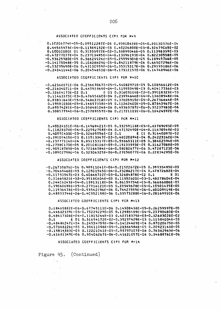
206

ASSOCIATED COEFFICIENTS C(P) FOR M=9

0 .102C67746-05 -0 .39 5122876-05 0 .93910438E-05-0 .20130376E-04 0 .44565973E-04-0 .11389132E-03 C .40226800E-03-0 .32679C65E-02 0 . lOCOCOOOE 01 0 .31555972E-02-0 .38899046E-03 0 .11398359E-03

-0 .47277077E-04 0 .237C3495E-04-0 .13396193E-04 0 .82230558E-05 -0 .53625980E-05 0 .36629924É-05-0 .25954 504E-05 0 .18945766E-05 -0 .14175048E-05 0 .10828B29E-05-0 .84211879E-06 0 .66507296E-06 -0 .53239690E-06 0 .4313C959F-06-0 .3 5315317E-06 0 .29193186E-06 -0 .24341144E-06 0 .20454853E-06-0 .17312157E-06 0 .14748946E-06

ASSOCIATED COEFFICIENTS C(P) FOR M=1C

-0 .6236E071E-06 0 .23667067E-05-0 .54082971E-05 0 .10856612E-04 -0 .21604071E-04 0 .4609Î869E-04-0 .11555349E-C3 0 .40417336E-03 -0 .326E4173E-02 0 .1 E 01 0 .31603116E-C2-0 .39018323E-03

0 .11463375E-03-0 .4769566CE-04 0 .23994646E-04-0 .13608548E-04 0 .83831643E-05-0 .54863718E-05 0 .37605915E-05-0 .26736644E-05 0 .19581030E-05-0 .14697 338E-05 0 .11262400E-05-0 .87843967E-06 0 .69574281E-06-0 .55848104E-06 0 .45363787E-06-0 .37237983E-06 0 .30857794E-06-0 .25789557E-06 0 .21721103E-06-0 .18424597E-06

ASSOCIATED COEFFICIENTS C(P) FCR M=l l

0 .40024351E-06-0 .14969421E-05 0 .33259118E-C5-0 .63789093E-05 0 .U828378E-04-0 .22592758E-04 0 .47132490E-04-0 .11670549E-03 0 .4055C430E-03-0 .32685556E-02 0 .1 E C l 0 .31640097E-02

-0 .39109415E-03 0 .11513347E-03-0 .48C20894E-04 0 .24223360E-04 -0 .13777114E-04 0 .85115317F-05-0 .55865311E-05 0 .38402594E-05 -0 .2738C170E-05 0 .201C8116E-05-0 .15133593E-05 0 .11627088E-05 -0 .90918785E-06 0 .72186584E-06-0 .58C82677E-06 0 .47287123E-06 -0 .38902798E-06 0 .32 30632 5E-06 -0 .27056077E-06 0 .22834295E-06

ASSOCIATED COEFFICIENTS CIP) FOR M=12

-0 .26735876E-06 0 .96911041E-06-0 .21522672E-C5 0 .39935495E-05 -0 •70469468E-05 0 .12501545E-04-0 .23286217E-04 0 .47872682E-04 - 0 . 1 17 53547E-03 0 .40646722E-03-0 .32684 878E-C2 0 .1 E 01

0 .3166982 IE-02 -0 .3918C604E-03 0 .11552600E-03-0 .48278604E-04 0 .244C6243E-04-0 .13913118E-04 0 .86159754E-C5-0 .56686806E-05 0 .39060698E-05-0 .27916121E-05 0 .20549678E-C5-0 .15501475E-05 0 .119 36478E-05-0 .93 54 2296E-06 0 .74427555E-06-0 .60009519E-06 0 .4 89 53744E-06-0 .4C352198E-06 0 .33573288E-C6-0 .28169910E-06

ASSOCIATED COEFFICIENTS C(P) FOR M=13

0 .18465862E-06-0 .6774 5111E-06 0 .14508438E-05-0 .26259597E-05 0 .44682339É-05-0 .75229229E-05 0 .12985489E-04-0 .23790480E-04 0 .48417308E-04-0 .11815244E-03 0 .40718375E-03-0 .32 683028E-02 0 .1 E 01 0 .31694172E-02-0 .39237429E-03 0 .11584004E-03

-0 .484 86247Ë-04 0 .24 554759E-04-0 .14C24409E-C4 0 .87020675E-05 -0 .57368228É-05 0 .39611C98E-05-0 .2 8366 586E-C5 0 .20923143E-05 -0 .15814383E-05 0 .12201041E-05-0 .95797107E-06 0 .76362963E-06 -0 .61681349E-06 0 . 50406267E-06-0 .41621057E-C6 0 .34688761E-06

ASSOCIATED COEFFICIENTS C(P) FOR M=14

Figure 45. (Continued)

207

-0 .13119653E-06 0 .47815102E-06-0 .101137436-C5 0 .179575626-05 -0 .297251C0E-05 0 .48149970E-05-0 .787271496-C5 0 .133443606-04 -0 .24168209E-04 0 . 48829331 E-04 ->0 . 11862 304E-C3 C .407729936-03 -0 .3268C548E-02 0 .1 E 01 0 .317145066-02 -0 .392835416-03

0 .11609520E-03-0 .46656004E-04 0 .24677C066-C4-0 .141166166-04 0 .87737730E-05-0 .57940756E-05 0 .40075296E-05-0 .28748804E-05 3 .21241700E-05-0 .16082623E-05 0 .12428927E-05-0 .977482456-06 0 .78045051E-06-0 .6314G560F-06 0 .516795406-06 -0 .427401176-36

ASSOCIATED C0EFFICI6NTS C(P) FOR M=15

0 .9 54 99650E-07-0 .34621770E-06 9 .72510024E-C6-0 .126811836-95 0 .2054 5635E-05-0 .32313812E-05 0 .50749197E-C5-0 .813672356-05 0 .136175C5E-04-0 .24458246E-04 3 .49148390E-C4-0 .11898992E-C3 0 .40815476E-03-0 .32977821E-02 0 .1 E C l 0 .31731677E-02

-0 .39321474E-03 0 .11630541E-03-0 .48796586E-C4 0 .247788136-04 -0 .141937C5E-04 0 .88343285E-05-0 .58425268E-C5 0 .40470487E-05 -0 .290 75807E-35 0 .21515522E-05-C .1631423 5E-C5 0 .12626547E-95 -0 .99447264E-06 0 .79515775E-06-0 .64421813E-06 0 .52805052E-06

ASSOCIATED COEFFICIENTS CIP) FCR M=16

-0 .70991776E-07 0 .25626478E-06-0 .53242308E-06 0 .919888356-06 -0 .14651704E-05 0 .22 518C49E-05-9 .342892 39E-C5 0 .527426756-05 -0" . 8 34 059 5 7 E -0 5 0 . 13830C28E-04-C .2468564 1E-C4 0 .494C0342E-04 - 0 . 11928 118E-03 0 .4C84 9C95E-03-D.32674916E-02 0 .1 E 01

0 .31746334E-02-0 .39 353111E-03 0 .116480726-03 -0 .489142946-04 0 .24864170E-04-3 .1425920CE-04 C .68857432E-05-0 .56 8391626-35 0 .40809638E-05-0 .29357684E-05 0 .2 17525586-C5-0 . 16515555E-35 0 .127 98996E-3 5 -0 .1C093570E-05 9 .8C8C96436-06 -0 .65 5576006-06

ASSOCIATED COEFFICIENTS CIP) FCR M=17

0 .5375323IE-07 -0 . 19 3351096-06 0 .39907574E-06-9 .68 268 3606-96 0 . 10724533E-05—0. 16180954E-05 0 .24047839E-O5-O. 35826599Ê-95 0 .54302619E-05-0 .850115266-05 C .1399853 IE-C4-Û.24867156E-04 0 .49602693E-94-0 .11951621E-03 0 .40876C60E-C3-0 .32672006E-92 0 .1 E 01 0 .31758987E-02-0 .39379806E-03 0 .11662 8426-03

-0 . 490 13052E-04 0 .2 4937284E-04-0 .14314961E-04 0 . 892981106-05 -0 .59195486E-05 0 .4110 28 30E-05-0 .296023 3 3E-C5 0 .219590906-95 -0 .16691625E-05 0 .12950393E-05-9 .10224799E-C5 0 .819605956-96

ASSOCIATED COEFFICIENTS CIP) FCR M=18

-0 .41367114fc -C7 0 . 14 83 5691E-G6-0 .3C4 53 978E-06 0 .516699426-96 -0 .80255068E-06 0 . 11928 196E-05-0 .17 3847636-0 5 0 .252545266-05 -0 .370444256-05 0 .55544913E-05-0 .86297669E-05 0 .141343276-04 -3 .250 14288E-04 0 .4S76 75 99E-04-0 .1197C833E-C3 0 .408979586-03 -0 .3266S141E-02 0 . 1 E 01 C . 3 1 770C91E-C2 - 9 .394C2548E-C3

0 .11675 158E-C3-0 .49098829E-04 0 .249996546-C4-0 . 14 3629336-04 0 .896 78749E-05-0 .59 5C44 37E-05 0 .4 1357993E-05-0 .29816038E-05 0 .2214C143E-0 5 -0 . U846553E-05 0 . 1 3C84196E-C5-3 . 10342040E-05

ASSOCIATED COEFFICIENTS CIP) FCR M=19

Figure 45. (Continued)

208

0 .32298291E-C7-0 .11554629E-06 0 .23609492E-C6-0 .39782400E-06 0 .6121C535E- n 6-0 .8S855101E-06 0 . I2888695E-C5-0 .18346143E-05 0 .26221241E-05-0 .38 024346E-05 C . 56549583E-05-0 .87343376E-C5 0 . 14245330E-04-0 .25135190E-04 0 .499C3 721E-C4-0 .11986 745E-03 0 .40916019E-C3-0 .32666418E-Q2 0 .1 E CI 0 .31779769E-02

-0 .39420767E-03 0 .11686188E-03-0 .49 171894E-C4 0 .25C53481E-04 -0 .14404489E-04 0 .9C009709E-05-0 .59774C25E-05 0 .41581437E-C5 -0 .30C03829E-05 0 .22299836E-05-0 .16983835E-05 0 .132C4374E-05

ASSOCIATED COEFFICIENTS CIP) FCR M=2C

-0 .25545828E-07 0 .91196038E-07-0 .18561314E-06 0 .31C94516E-06 -0 .474644C8E- -6 0 .68957399E-C6-C .97612236E-C6 0 .13664585E-05 -0 .19124433E-05 0 .27006611E-05-0 .3 8823861E-05 0 .57373140E-05 -0 .88204696E-05 0 .14337201E-04-0 .25235701E-04 0 .50017335E-04 -0 .12CCC051E-03 0 .40930S46E-03-0 .32663678E-C2 0 .1 E 01

0 .31786341E-02-0 .39439C28E-03 0 .11695521E-03-0 .49235269E-04 0 .25100296E-04-0 .14440746E-04 0 .90299393E-05-0 .60010767E-05 0 .41778308E-35-0 .30 169900E-05 0 .22441783E-05-0 .17108009E-05

PE*= PECLET NUMBER/2 = 0 . 50

EIGENVALUES

-0 .10222366E 0 1-0 .25 941912E 01 - 0 . 41621720E 01 -0 .57311C05E 01 -0 .7 3006545E 01 -0 . 887C5770E 01 -0 .10440729E 02 -0 .12011032E 02 -0 .135 8143 7E 02 -0 . 1515 1918E 02 -0 .16722453E 02 -0 . 18293032E 02 -0 .19863642E 02 -0 .21434277E 02 -0 .23Û04935E 02 -0 .24575610E 02 -0 .26146 295E 02 -0 .27716997E 02 -0 .29287707E 02 -0 .30858422E 02

EXPANSION COEFFICIENTS ' A(M

0 .211132C3E 00 -0=61495615E-Ol 0 .3 1378591E-01-0 .19709586E-01 0 .13817566E-01-0 . 10 367709E-01 0 .8 1465061E-02-0 .66183913E-02 0 .55144945fc -02 -0 .46865349E-02 0 .40468038E-C2-0 .35404103E-02 0 .31314751E-Q2-0 .27956286E-02 0 .25158295E-02-0 .22798287E-02 0 .20786526E-02-0 . 19056616E-02 0 . 1756308 1E-02 -0 . 16379987E-02

2«A( f ) / ( J1 (M)»J1 (M))=T0TAL COEFFICIENT

0 .15667600E 01 -0 .10622827E 01 0 .85167994E CO-O.72947704E 00 0 .647778C1E 00 -0 .58837063E 00 0 .54271926E 00 -0 .50623719E 00 0 .47622660E 00 -0 .45097S03E 00 0 .42935887E C0-0 .41057386É 00 0 .39405693E 00 -0 .37938660E 00 0 .36624608E 00 -0 .35439089E 00 0 .34363432E 00 -0 .33384425E 00 0 .32501376E 00 -0 .31928638E 00

ASSOCIATED COEFFICIENTS C(P) FOR M=1

0 . 1 E 01 0 .19622208E-01-0 .17544691E-G2 0 .40270444E-03 -0 .134 92395E-0 3 0 .56268852E-04-0 .27115697E-C4 0 .14485023E-04 -0 .83597546E-05 0 .51241512E-05-Q.32961832E-C5 0 .22058808E-05 -0 .15257945E-05 0 .10853424E-05-0 .79C81301E-06 0 .58835373E-06 -0 .44579871E-06 0 .34328C79E-06-0 .26816 334E-06 0 . 212 19540E-06 -0 .169 86505E-06 0 .13741487E-06-0 .11222985E-06 0 .92463890E-07 -0 .76791246E-37 0 .64 246 714E-07-0 .54118489E-07 0 .45875256E-07 -0 .39116087E-07 0 .33535311E-07-0 .28897750E-07 0 .25021205E-07

Figure 4$. (Continued)

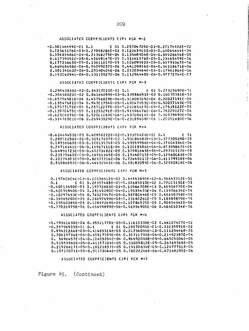
209

ASSOCIATED COEFFICIENTS CIP) FCR M=2

- 0 .30144499E-C1 0 .1 E 01 0 .25704705E-0 1 -0 .27174922E-02 0 .72363176E-03-O.27058286E-03 0 .12263915E-03-0 .Ô3064644E-D4 0 .35485486E-04-0 .21368275E-04 0 .13568 904E-04-0 .89928654E-05 0 .617 39392E-05-0 .4265914 7E-05 C .31661576E-05-0 .23465459E-06 0 .17723663E-05-0 . 13611817E-05 0 .1C609 55 2E-0 5 -0 .83793367E-06 0 .66968498E-06-0 .54099037E-06 0 .44129 816E-06-0 .36 318671E-06 0 .30134160E-06-0 .25190404E-06 C .21203464E-C6-0 .17 961864E-06 0 .153C6294E-06-0 .13115527E-06 C .11296440E-06-0 .97 772764E-C7

ASSOCIATED COEFFICIENTS C(P) FCR M=3

0 .29543835E-02-0 .34337C10E-01 0 . 1 E 01 0 . 27323690E- - ) ! - 0 .30458022E-02 0 .86164059E-03-0 .33936691E-03 0 .16070381E-03 -0 .85754581E-04 0 . 49 796829E-04 - 0 . 3 C 8 0 8 3 0 5E-04 0 . 20027191E-04 -0 .13547681E-04 0 .94 7C1754E-05-0 .68C47653E-05-0 .53057143E-05 -0 .3 75 7717 2E-05 0 . 2 8712277E-05-0 .2 2283 4 2 7 E -C5 - 0 . 175J5 I22E-05 -0 .13970475E-05 0 . 11255291E-05 - 0 . 9 I 596676E-C6 - 0 . 75229127E-06 -0 .623C6076E-06 0 . 5 2 0 C 1 C 6 9 E -C6 - 0 . 43 7 C 8 6 1 4 E - 0 6 0 . 36979493E - 0 6 -0 .31476501E-06 0 .26943829E-C6-C .23185608 E -C6 C .2 0 351830E-96

ASSOCIATED COEFFICIENTS CIP) FCR M=4

-0 .62449452E-03 0 .4C858 222E-02-C . 3 53C14C6E-01 0 .1 E 01 0 .28001258E-01-0 .31917837E-02 0 .93G8648 2E-03-D.377 30529E-03 0 .183 36660E-03-0 . ICO13974E-03 0 .59359956E-C4-0 .374C4334E-04 0 .24716441E-04-0 .1696711CE-04 0 .12C18306E-C4-0 .87395847E-05 0 .64991723E-05-0 .4Ç273482E-05 C .37991645E-05-C .29731117E-C5 0 .23575460E-C5-0 .18916345E-05 0 .1534CC15E-C5-0 .12560C63E-C5 0 .10374303E-05-0 .86377716E-06 0 .72449211E-06-0 .61179318E-06 0 .51986850 E-0 6? -0 .44432943E-06 0 . 3 81 83059E-06-0 . 32 982818E-06

ASSOCIATED COEFFICIENTS C(P) FOR M=5

0 .1976C8C4E-C3-0 . 1C038912E-02 0 = 4454 3 895E-02-0 .35643312E-01 0 .1 E 01 O .20357488E-OÎ -O .326850ÎOE-O2 0 .97CC3150E-03

-0 .40013490E-03 0 .19772883E-03-0 .10966708E-C3 0 .65938775E-04 -0 .4 2094540E-04 0 .28149Û90E-04-0 . 19535453E-04 0 .13976634E-04 -0 .10257493E-04 0 .76 92794 7E-05 -0 .58780446E-C5 0 .45650758E-05 -0 .35965200E-05 0 .28697499E-05-0 .2 3160261E-C5 0 .18883809E-05 -0 .15540385E-05 0 .12897269E-05-0 .10786575E-05 0 .90854362E-06 -0 .77026975E-06 0 .65 6S9899E-06-0 .5 63 54905E-06 0 .48601034E-06

ASSOCIATED COEFFICIENTS CIP) FOR M=6

-0 .79361630E-04 0 .35521770E-03-0 .11613338E-C2 0 .46127427E-02 -0 .35796933E-01 0 .1 E 01 0 .28572055E-C1-0 .33135591E-02

0 .99421266E-03-0 .41485314E-03 0 .2C734094E-C3-0 .11625446E-03 0 .70619 736E-04-0 .45517559E-04 0 .30711790E-04-0 .21492357E-04 0 . 5496457E-04-0 .11455354E-04 0 .86492048E-0 5 -0 .665C5004E-05 0 .5195394OE-O5-0 .41157104E-05 0 .33009812E-05-0 .26769768E-05 0 .21926417E-05-0 .18121837E-05 0 .15100634E-C5-C .12677731E-05 0 .10717071E-05-0 .91173064E-05 0 .78022248E-06-0 .67148290E-06

ASSOCIATED COEFFICIENTS CIP) FCR M=7

Figure 45. (Continued)

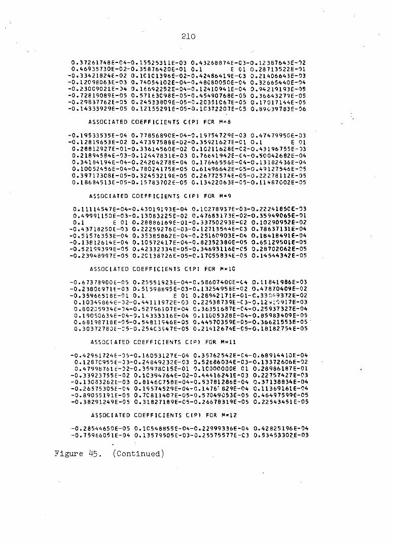
210

0 .37261748E-04-0 .15525311E-03 0 . 43268874E-03-0 .12387643E-02 0 .46935730E-02-0 .35876420E-01 0 .1 E 01 0 .28713522E-01

-0 .33421824E-02 0 . ICIC1396E-02-0 .42486419E-C3 0 .21406643E-03 -0 .12098063E-03 0 .74054102E-04-0 .4 8C80050E-04 0 .32665440E-04 -0 .23009021E-04 0 .16692252E-04-0 .12410941E-04 0 .94219193E-05 -0 .72819089E-05 0 .57163C98E-05-0 .45490768E-05 0 .36643279E-05 -0 .29837762E-05 0 .24 533809E-O5-O.2035ÎO6 7E-05 O .17017144E-05 -0 .14333929E-05 0 .12155291E-05-0 .1C372207E-C5 0 .89Û39783E-06

ASSOCIATED COEFFICIENTS CIP) FCR M=8

-0 .19533535E-04 0 .77856890E-04-0 .19754729E-03 0 .4747995CE-03 -0 .128 19653E-02 0 .47397588E-02-0 .35921627E-C1 0 .1 E 01

0 .28812927E-01-0 .33614560E-02 0 .10211628E-C2-0 .43196 7 55E-03 0 .21894584E-03-0 .12447831E-03 0 .76641942E-C4-0 .50042682E-04 0 .34184194E-04-0 .24204278E-04 0 .17646 55 6E-04 -0 .13 1 824 36E-04 0 .100 52456E-04-0 .78024175E-05 0 .6149664 2E-C5-0 .49127546E-05 0 .39717308E-05-0 .32453219E-05 0 .2 6772 574E-05-0 .22 278112E-05 0 .186 84513E-05-0 .15 78 3702E-05 0 .13422063E-C5-0 .11487002E-05

ASSOCIATED COEFFICIENTS CIP) FOR M=9

0 .11114547E-04-0 .43019193E-04 0 .10278937E-03-0 .2224185CE-03 0 .4 9991150E-0 3 -0 .13083225E-02 0 .47683Î7 3E-O2-O.35949O65E-OÎ 0 .1 E 01 0 .28886169E-01-0 .33750293E-C2 O .10290952E-02

-0 .43718250E-03 O .22259276E-03-0 .12713 544E-C3 0 .78637131E-04 -0 .51576353E-04 O .35385862E-04-C .2516C903E-04 O .18418491E-04 -0 .13612614E-04 0 .10572417E-04-0 .82352380E-05 0 .65129501E-05 -0 .52199399E-05 0 .42332334E-05-0 .34693H6E-E5 0 .28702062E-05 -0 .23948997E-05 0 .20138726E-05-0 .17C55834E-05 O .14544342E-05

ASSOCIATED COEFFICIENTS CIP) FCR M=1C

-0 .67378900E-C5 O .25551923E-04-C .58607400E-C4 O .11841986E-03 -0 .23806971E-03 0 .5159 8895E-03-0 .13254958E-02 0 .47870409E-02 -0 .3 5966518E-01 0 .1 , E 01 0 .28942171E-01-C .33049372E-02 0 . 103498641-32 -0 .44111972E-03 0 .22538739E-C3-0 .12Vl9917E-03 0 .80205934E-04-0 .52796107E-04 C .36351687E-C4-0 .25937327E-04 0 .190 50 634E-C4-9 .14333316E-04 0 .11Û05328E-04-0 .85 983409E-05 0 .68198718E-05-0 .54 811946E-05 0 .44570359E-05-0 .36621553E-05 0 .303 72780£- :5 -0 .2 54C3S47E-05 0 .21412674E-05-0 .18182754E-05

ASSOCIATED COEFFICIENTS CIP) FCR M=l l

- 0 .4 2961724E-05-0 .16053127E-04 0 .35762 542E-04-0 .68914410E-04 0 .128 7C95 5E-3 3 -0 .24 8492 32E-C3 0 .526 66034E-C3-0 .13 372606E-02 0 .47998761E-02-0 .35978C15E-01 0 .10000000E C l 0 .28986187E-01

-0 .33923755E-02 0 .1C394764E-02-0 .44416241E-03 0 .22757427E-03 -0 .13083262E-03 0 .8146C758E-04-0 .53781286E-04 0 .37138834E-04 -0 .26575305E-04 0 .19574529E-04-0 .1476 ' 829E-04 C .11369161E-04 -0 .890 55191E-0 5 0 .7C811407E-05-0 .57049C53E-05 0 .46497599E-05 -0 .38291249E-05 0 .31827189E-05-0 .26678319E-05 0 .22543451E-05

ASSOCIATED COEFFICIENTS C(P) FOR M=12

-0 .28544650E-05 0 .1C548855E-04-0 .22999336E-04 0 .42825196E-04 -0 .75966051E-04 0 .13579505E-03-0 .25575577E-C3 0 .53453302E-03

Figure 45. (Continued)

211

-0 .13456422E-02 0 .46089818E-02-0 .35965701E-01 0 . lOCCOOOOE 01 0 .29021695E-01-0 .33980977E-02 0 .10429749E-02-0 .44 656112E-03 0 .2 29 31673E-03-0 .13214688E-03 0 .82479564E-04-0 .54 58 7886E-04 0*37788104E-04-0 .271C5952E-04 0 .2CC12954E-04-0 .15133911E-04 0 .11677590E-04-0 .91674477E-05 0 .73C51651E-C5-0 .58 977524E-05 0 .481675876-0 5 -0 .39745737E-05 0 . 33102265E-05-0 .27813891E-05

ASSOCIATED COEFFICIENTS C(P t FCR M=13

0 .19626341 E-05 -0 .71918650E-05 0 .15425204E-04-0 .27 993602E-04 0 .4 7821288E-04-0 .8C965478E-04 0 .14C86290E-03-0 .261C0761E-03 0 .54013835E-03-0 .13518068E-02 0 .48156301E-C2-0 .35990990E-01 O. IOOOCOOOE 01 0 .29050810E-01-0 .34025912E-C2 0 .10457510E-02

-0 .44848398E-03 0 .23072670E-03-0 .13321953E-03 0 .83317597E-04 -0 .55255823E-04 0 .38330327E-04-0 .27551442E-C4 0 .20383396E-94 -0 .15445024E-04 0 .11941156E-04-0 .93924538E-05 0 .74985903E-05 -0 .6065C919E-05 0 .49624307E-05-0 .41C23165E-05 0 .34245103E-05

ASSOCIATED COEFFICIENTS C(P> FCR M=14

-0 .13890474E-05 0 .50563537E-05-0 .10707280E-C4 0 .19051064E-04 -0 .31631430E-04 0 .51455586E-04-0 .84623954E-C4 0 .14460400E-03 -0 .26492098E-03 0 . 54435031E-03-0 .13564598E-C2 0 .48205969E-02 -0 .35994631E-01 0 .1C0C0C00E 01 0 .29C75164E-C1-0 .34061812E-02

0 .10475890E-02-0 .4 5004845E-03 0 .23188334E-03-0 .13410599E-C3 0 .84C 14 217E-C4-0 . 55816C79E-04 0 .3 8787037E-04-0 .27929C25É-04 0 .206 99091E-04-0 .15711541E-04 0 .12166C69E-C4-0 .95 871155E-05 0 .7 6667429E-0 5 -0 .62113365E-05 0 .5C9C6970E-05-0 .42177319E-05

ASSOCIATED COEFFICIENTS CIP) FOR M=15

0 .10077435E-05-0 .36489735E-05 0 .764 89 719E-05-0 .13399319E-04 0 .21761378E-04-0 .34338916E-04 0 .54169883E-04-0 .87 374925E-04 0 .14743987E-03-0 .26791136E-03 0 .54 759C59E-0 3 -0 .13600495E-02 0 .48243789E-02-0 .35997185E-01 0 .1 E C l C .29C95802E-01

-0 .3409C9C1E-02 0 .10498186E-02-0 .45133797E-C3 0 .23284350E-C3 -0 .13484530E-03 0 .84601360E-04-0 .56289531E-04 0 .39175389E-04 -0 .28251759E-04 0 .20970263E-04-0 . I 5941564E-C4 0 .12364831E-04 -0 .97567150E-05 0 .78140442E-05-0 .63405374E-05 0 .52078293E-05

ASSOCIATED COEFFICIENTS CIP) FOR M=16

-0 .74695545E-06 0 .26930954E-05-0 .55991238E-C5 0 .96867273E-05 -0 .15458531E-04 O .2382O3Î9E-O4-O.36398462E-O4 0 .56245012E-04 -0 .89492177E-04 0 .14 963606E-03-0 .27C24 515E-03 0 .55013333E-03 -0 .13628701E-02 0 .48273081E-02-0 .3 5998904E-01 0 .1 E 01

0 .29113456E-01-0 .34114802E-02-0 .10513332E-C2-0 .45241273E-03 0 .23364605E-03-0 . I 3547191E-03 O .65099OÎ5E-04-0 .5669342OE-O4 0 .39508326E-04-0 .28529745E-04 0 .21204912E-04-0 .16141518E-04 0 .12536684E-04-0 .9S05697 3E-05 0 .79447284E-05-0 .64601957E-05

ASSOCIATED COEFFICIENTS CIP) FOR M=17

0 .5641330 5E-06-0 .2C26 7835E-05 0 .41855550E-C5-0 .71678680E-05 0 .11278003E-04-0 .17052052E-04 0 .2 5412805E-C4-0 .37996940E-04 0 .57864288E-04-0 .91154542E-04 0 .15137494E-C3-0 .27210006E-03 0 . 55216353E-03-0 .1365 1241E-02 0 .4 8296117E-02-0 .360C0149E-01

Figure 45. (Continued)

212

0 .1 E 01 0 .29128692E-01-0 .34134648E-C2 0 .10525993E-02 -0 .45331040E-03 0 .23433107E-03-0 .13600425E-03 0 .855249C8E-04 -0 .5704C727E-04 0 .3979 5927E-04-0 .2 877C952E-04 0 .214C9428E-04 -0 .16316639E-04 0 .12688131E-04-0 .10038572E-C4 0 .80680196E-05

ASSOCIATED COEFFICIENTS CIP) FOR M=18

- 0 .43316004E-06 0 .15516757F-05-0 .31865407E-05 0 .54113313E-05 -0 .8415S462E-05 0 .12530232E-04-0 .183C3362E-04 0 .26665894E-04 -0 .3926G037E-04 0 .591504 87E-04-0 .92482386E-C4 0 .15277CC1E-03 -0 .27359732E-03 0 .5538C770E-03-0 .13669463E-02 0 .48314315E-02 -0 .3600C891E-01 0 .1 E 01 0 .29142119E-01-0 .3415134CE-02

0 .10536476E-02-0 .45408621E-03 0 .23491401E-C3-0 .13 646138E-03 0 •85892279E-04-0 .57341636E-04 0 .4C046188E-C4-C .28981792E-94 0 .21589106E-C4-0 .16471570E-04 0 .12824130E-04-C .10167041E-04

ASSOCIATED COEFFICIENTS CIP) FCR M = 1 S

0 .33751637E-06-0 .1206C838E-05 0 .2 46 52327E-05-0 .4157C81CE-05 0 .64031727E-C5-0 .94132219E-05 0 .13527279E-04-0 .19 300516E-04 0 .27667611E-04-0 .40274136E-04 C .60188218E-04-0 .93559172E-04 0 .1539C682E-03-0 .27482273E-03 0 .55515693E-C3-0 .13684401E-02 0 .4 8328970E-02-0 .360C1385E-01 0 .1 E C l 0 .29153897E-01

-0 .34164425E-02 0 . IC545797E-02-0 .454 74496E-03 0 .23541590E-03 -0 .13685680E-03 0 .86211475E-04-0 .57604235E-C4 0 .40265607E-04 -0 .29167658E-04 0 .21748798E-04-0 .16611895E-04 0 .12959966E-04

ASSOCIATED COEFFICIENTS C tP ) FCR M=2C

-0 .26646988E-06 0 .95021808E-06-0 .19345302E-05 0 .32428381E-05 0 .49545886E-05 0 .72068757E-04-0 .10217464E-C4 0 .14331152E-04

-0 .20106259E-04 0 .28479900E-04-0 .41C99951E-04 0 .61037152E-04 -0 .94444104E-04 0 .15484524E-03-0 .27583800E-C3 0 .55627795E-03 -0 .136968C3E-03 0 .48340931E-02-0 .36001742E-G1 0 .1 E O l

0 .29162412E-01-0 .34177577E-02 0 .10553649E-02-0 .45 531456E-03 0 .2 35 85168E-0 3 -0 .1372C159E-03 0 .86491060E-04-0 .57835348E-04 0 .40459890E-04-0 .29333860E-04 0 .21895154E-04-0 .16758336E-04

PE*= PECLET NUMBER/2 = 5 .00

EIGENVALUES

-0 .3372C255E 01 -0 . 15383S55E 02 -0 .29751720E 02 -0 .44738275E 02 -0 .59986350E 02 -0 .75375C50E 02 -0 .9C848950E 02 -0 .10637875E 03 -0 .12195995E 0 3 -0 .1375585CE 03

EXPANSION COEFFICIENTS: A(K)

0 .19534415E 00 -0 .55077742E-01 0 .29345738E-01-C .18917481E-01 0 .13388522E-01-0 . ICO 61661 E-01 0 .7 89 568 85E-02-0 .64 048154E-02 0 .53379298E-0 2 -0 .464 85834E-02

2»A(NÏ / ( J1 IM)»J I (M) )=T0TAL COEFFICIENT

0 .14496020E 01 -0 .95141955E OC 0 .7965C410E 00 -0 .70016022E 00 0 .62766410E 00 -0 .571CC231E 00 0 .52600983E C0-C .48990088E 00 0 .46097861E 00 -0 .44 732701E 00

Figure 45. '(Continued)

213

ASSOCIATED COEFFICIENTS C(P) FCR M=1

0 . 1 E 01 0 .70453186E- 01 -0 .4 7637498E-0 2 0 . 11467747E-02 - 0 . 39173232E-03 0 . 16516730É- 03 - C .80155395E-C4 0 . 43037231E-04 - 0 . 24942905E-34 0 . 15349964E- 04 - 0 .99163851E-05 0 . 66696934E-05 - 0 . 4 6423813E-05 0 .3329G525E- 05 - 0 .24515176E- C5 0 . 18497097E-05 - 0 . 1427S936E—05 0 . 11273794E-05 - C .91C51523E-•06 0 . 75 328841E-06

ASSOCIATED COEFFICIENTS CIP) FCR M=2

- 0 . 1231181 IE 00 0 .1 E 01 0 .17203675E 00 -0 . 78375442E- 02 0 . 29563335E-02- 0 .11918939E-02 0 .56296335E- C3- 0 . 296954C9E-•03 0 . 169912C6E-03- 0 .1C348423E- 03 C .66220385E-•C4-•0 . 441C6C35E- 04 0 . 30362073E-04-•0 .21483353E- 04 0 .15555140E- 04- C . 11481765E-•04 0 . 86107743E-05-•0 .65398638E-05 0 .50130755E- 05-• c . 38627371E-•05

ASSOC I ATED COEFFICIENTS C(P) FCR M=3

0 . 31233951E—91-•0 .202C2309E 00 0 .1 E 01 0 . 22 820495E 00 - 0 . 6515C2S4E-02 0 .3S463332E-02-•C .17279009E-•02 0 . 87C08669E-•03 - 0 . 48262086E-03 0 .28765475E-03-•0 .1612328 3E-•C3 0 . 11933328E-•03 - 0 . 81444358E—04 0 .57255984E- 04-•0 .41257656E-•04 0 . 30349902E-•04 - 0 . 2 27 1228 7E-04 0 .17235178E-04-•0 .13219447E-•04 0 . 10211080E-•04

ASSOCIATED COEFFICIENTS C(P) FOR M = 4

- 0 . 96312291E-02 0 .53 573301E- 01 --0 .23737391Ê 00 0 . 1 E 01 0 . 2 5952025E 00 -•0 .451S3062E- 02 0 .45C60190E--02 -•0 . 20568179E-•02 0 . 10757189E—02-•0 .61536989E- 03 0 .37625343E--03 -•0 . 24211047E-•03 0 . 1621S057E-03--0 . 1122C986E- 03 0 .79671256E--04 -•0 . 57750621E-•04 0. 42533385E-04--0 .31676S57E- 34 0 .23726037E--04 -•9 . 17744C43E-•04

ASSOCIATED COEFFICIENTS , C (P ) FCR M=5

0. 34469133E-32--0 .17092418E-•01 0 .63S55504E--C 1 -- 0 . 25 668892 E "0 0. 1 E 01 0 .27874884E 00 --C .27C82954E--02 9 . 48 5G5916E-- n 2

— 0. 22671013E-02 3 . 12173903E- 02--C .71301311E--03 c. 44561982E--93 — 3 . , 29289268E-33 0 .2C044916E-•03 --0 .14183875E--03 0, 10 324587E-- n 3 -0. 77C25379E-04 0 .5874C284E-•34 --0 .45711667E--C4 0. , 3 6267835E--94

ASSOCIATED COEFFICIENTS C(P) FCR M=6

-0 . , 141U632E-02 0 .6419C212E--02 --0 .2C661104E--CI 0. , 69 753C06E--91 -0 . , 26887759E 00 0 .1 E 01 0 .29158686E CO--0. , 11799194E--02 0. , 50642078E-C2--0 .2 3947227E--02 0 . 13056534E--02 -- c . , 77412481E--93 0. . 48839948E-03--0 .32308333E--03 0 .221775G9E--C 3-- 0 , , 1567461CE--03 0 . . 1 13363C4E-03--0 .83443762E--04 C .62184818E--C4--9 , . 46 644227E--04

ASSOCIATED COEFFICIENTS C (P ) FCR M = 7

0 , . 65CC78C4E-C3--0 . 2 7 744867E--02 C .79357351E -02 --0 , . 22 646388E--91 0 , . 73464349E-01 -0 .27732773E 00 0 .1 E C 1 c , . 30C74747E 90 0, . 845653 8 9E-0 4 0 .52077111E--02 -0 .24778969E -C2 9 , . 13650436E -92

-0 . . 8 1595836E-0 3 0 .51786373E--03 -0 .3 43 73 62 3E -C 3 0, . 23 599508E -93 -0 . 16612124E-03 0 .118S5C12E--03 -0 .8593C404E -04 0, . 61986692E -04

ASSOCIATED COEFFICIENTS CIP) FCR M = 8

Figure 45. (Continued)

214

- 0 . 3 3 0 4 6 0 5 9 E - 0 3 0 . 1 3 4 7 4 4 2 4 E - 0 2 - 0 . 3 5 3 1 0 5 4 9 E - C 2 C . 8 8 o 1 8 5 2 3 E - 0 2 - 0 . 2 3 9 0 5 8 4 1 E - 0 1 0 . 7 6 0 7 9 1 9 3 E - 0 1 - 0 . 2 8 3 5 8 7 6 6 E C C C . 1 E " 1

0 . 3 0 7 6 6 1 9 5 E 0 0 0 . 1 1 1 7 1 4 1 4 E - C 2 C . 5 3 2 5 3 0 5 C E - C 2 - 0 . 2 5 4 6 7 5 6 8 E - 0 2 0 . 1 4 2 C C 9 C 0 E - 0 2 - 0 . 8 5 8 7 7 5 1 C E - 0 3 C . 5 5 1 9 2 9 5 3 E - 0 3 - 0 . 3 7 1 5 8 6 0 7 E - 0 3 0 . 2 5 9 4 2 2 5 6 E - 0 3 - 0 . 1 8 6 4 1 4 5 5 F - C 3 0 . 1 3 7 C 6 2 8 3 E - C 3 - 0 . 1 0 2 6 0 0 3 7 E - O 3

A S S O C I A T E D C O E F F I C I E N T S C ( P ) F C R M = 9

0 . 1 8 8 6 5 8 4 5 E - 0 3 - 0 . 7 4 2 5 3 2 5 2 E - 0 3 C . 1 6 1 8 4 4 1 8 E - C 2 - : . 4 0 7 4 l 4 3 6 E - 0 2 0 . 9 5 0 9 6 3 5 3 E - 0 2 - 0 . 2 5 0 4 9 8 0 0 F - G 1 0 . 7 d 5 0 0 2 8 3 E - G l - C . 2 8 9 1 2 1 3 J E " 0 0 . 1 E 0 1 0 . 3 1 4 4 6 C 5 3 E O C 0 . 1 5 3 7 6 8 0 C E - C 2 C . 5 8 3 7 5 6 2 6 E - 0 2

- 0 . 2 9 8 2 7 9 8 6 E - 0 2 0 . 1 8 2 2 6 2 5 2 E - 0 2 - 0 . 1 2 4 3 6 5 0 9 E - C 2 0 . 9 3 0 1 2 7 2 2 E - 0 3 - 0 . 7 5 2 1 S 4 1 4 E - 0 3 0 . 6 5 0 7 8 4 8 2 f c - C 3 - C . 5 9 7 0 7 0 9 6 E - C 3 0 . 5 7 6 6 5 6 7 4 E - C 3

A S S O C I A T E D C O E F F I C I E N T S C ( P ) F C R M = 1 C

- 0 . 1 1 3 1 5 0 7 1 E - 0 3 0 . 4 3 4 5 9 4 7 5 E - 0 3 - C . I C 1 5 3 6 3 C E - C 2 0 . 2 1 C 9 7 4 8 9 E - 0 2 - 0 . 4 * 0 4 6 6 1 6 6 - 0 2 0 . 9 9 4 2 6 5 8 3 E - 0 2 - C . 2 5 7 7 8 5 2 O E - 0 1 0 . 8 0 1 6 0 4 0 7 E - 0 1 - 0 = 2 9 3 1 7 \ 4 5 E 0 0 0 . 1 E 0 1 0 . 3 1 9 1 5 7 9 9 E C O 0 . 2 1 5 6 5 9 0 6 E - 0 2

0 . 6 0 1 8 7 4 C 4 E - 0 2 - 0 . 3 1 - 2 4 0 1 2 3 E - 0 2 C . 1 9 5 2 7 7 7 9 E - C 2 - 0 . I 3 6 7 4 C 3 C E - 0 2 0 . 1 C 5 2 C 1 6 1 E - 0 2 - 0 . 8 7 6 2 2 C 4 2 F - 0 3 C . 7 8 1 2 2 P 4 4 E - C 3 - 0 . 7 3 8 3 5 4 2 5 6 - ^ 3

P E » = P E C L E T N U M B E R / 2 = 5 0 . C O

E I C E N V A L U E S

- 0 . 3 6 5 3 4 5 4 5 E 0 1 - 0 . 2 2 1 6 1 6 6 5 E 0 2 - C . 5 5 9 9 6 3 0 0 E 0 2 - 0 . 1 0 4 1 8 C 4 0 E 0 3 - 0 . 1 6 5 4 3 4 2 5 E 0 3 - 0 . 2 3 8 3 2 3 5 5 E 0 3

E X P A N S I O N C O E F F I C I E N T S : A ( Y )

0 . 1 8 6 6 4 5 8 6 E 0 0 - 0 . 4 4 6 9 5 5 5 0 E - 0 1 C . 1 9 6 4 7 1 5 6 E - C 1 - C . 1 0 7 1 8 5 9 6 E - 0 1 0 . 6 3 2 9 8 0 9 7 E - 0 2 - 0 . 4 1 6 3 5 7 6 C E - 0 2

2 « A ( f ) / ( J l ( M ) » J l ( M J ) = T O T A L C O E F F I C I E N T

0 . 1 3 6 5 C 5 4 0 E 0 1 - 0 . 7 7 2 C 7 6 3 4 E 0 0 0 . 5 3 8 6 9 2 9 1 E 0 0 - 0 . 3 9 6 7 0 8 9 7 E C O 0 . 2 9 6 7 4 6 2 S E C O - O . 2 3 6 2 8 4 2 C E 0 0

A S S O C I A T E D C O E F F I C I E N T S C ( P ) F C R M = 1

0 . 1 0 0 0 C 0 0 0 E 0 1 0 . 7 6 1 3 5 6 8 6 E - 0 1 - 0 . 5 C 1 0 6 9 8 1 E - C 2 0 . 1 2 1 6 4 1 6 1 E - 0 2 - 0 . 4 1 7 5 7 6 1 7 E - 0 3 0 . 1 7 6 2 7 4 2 C C - C 3 - C . 6 5 6 8 7 3 4 4 E - C 4 0 . 4 6 C 4 2 0 5 8 E - 0 4 - 0 . 2 6 6 9 9 8 3 9 E - C 4 0 . 1 6 4 3 9 4 2 7 E - 0 4 - 0 . 1 C 6 2 5 3 9 C E - C 4 0 . 7 1 5 C 3 4 7 2 E - 0 5 - 0 . 4 9 8 0 C 2 2 4 E - 0 5 0 . 3 5 7 3 9 0 2 4 E - 0 5 - 0 . 2 6 3 4 3 7 4 7 E - 0 5 0 . 1 9 9 0 1 5 7 5 E - 0 5 - 0 . 1 5 3 8 5 0 2 4 E - 0 5 0 . 1 2 1 7 4 8 2 5 E - 0 5 - 0 . 9 8 5 9 3 9 1 7 E - C 6 0 . 8 1 8 5 0 3 6 9 E - 0 6

A S S O C I A T E D C O E F F I C I E N T S C t P ) F O R M = 2

- 0 . 1 6 7 C 9 2 2 1 E 0 0 0 . 1 C 0 C C C 0 C E 0 1 0 . 2 5 C 6 7 6 7 0 E 0 0 - 0 . 4 3 3 9 9 8 6 7 E - 0 2 0 . 3 4 5 8 C 2 8 8 E - 0 2 - 0 . 1 4 5 1 7 3 1 7 E - 0 2 C . 7 C 2 7 4 1 6 4 E - C 3 - 0 . 3 7 6 2 4 0 8 2 E - 0 3 0 . 2 1 7 3 7 9 2 3 E - 0 3 - 0 . 1 3 3 2 6 6 7 2 E - 0 3 0 . 8 5 6 5 9 3 5 7 E - 0 4 - 0 . 5 7 2 1 8 4 3 9 E - 0 4 0 . 3 9 4 5 1 3 5 7 E - 0 4 - 0 . 2 7 9 2 5 6 6 5 E - 0 4 0 . 2 C 2 0 2 4 9 1 E - 0 4 - 0 . 1 4 8 7 7 9 9 7 E - C 4 0 . 1 1 1 1 2 1 1 6 E - 0 4 - 0 . 8 3 8 4 5 5 2 0 E - 0 5 0 . 6 3 6 2 7 9 5 7 E - C 5 - 0 . 4 8 2 7 7 2 2 7 E - 0 5

A S S O C I A T E D C O E F F I C I E N T S C l " ) F O R M = 3

Figure 45. (Continued)

215

0 .79249083E-01-0 .378C1625E 00 0 .1CC0000CE 01 0 .46968541E 00 0 • 249 2 728 2E-01 0 .55214234E-02-0 .23134757E-02 0 .12449186E-02

-0 .71889666E-03 0 .44020C74E-03-0 .28257569E-03 0 .18849897E-C3 -0 .129 77783E-03 0 .9 1708236E-04-0 .66207236E-04 0 .48626573E-04 -0 .36186762E-04 0 .27167C08E-04-0 .20467306E-C4 0 .15361899E-04

ASSOCIATED COEFFICIENTS CIP) FOR M=4

-0 .533521C7E-01 0 .23073C58E 00 -0 .60378129E 00 0 .100C0003E 01 0 .75938792E 00 0 . 1C1C7609E 00 0 .11737787E-01-0 .30238288E-02 C .18299421E-0 2 -0 .11213488E-02 0 .7 2022138E-03-0 .48082737E-03 0 .33155399E-0 3 -0 .2 3491873E-03 0 .17030238E-03-0 .12585738E-03 0 .94509150E-04-0 .71887314E-04 0 .55207760E-C4-0 .42645244E-04

ASSOCIATED COEFFICIENTS CIP) FOR M=5

0 .44389109E-01-0 .16239449E 00 0 .45664506E 00 -0 .89319692E CO O . IOOOCOOOE CI 0 .11864647E 01 0 .26148466E CO 0 .32252085E-01

-0 .32528638E-02 0 .26574511E-02-0 .16955997E-C2 0 .11330081E-02 -0 .78221732E-C3 0 .55548809E-03-D.40422687E-C3 0 .30048702E-03 -0 .2276C150E-03 0 .17529721E-03-0 .13705655E-03 0 .10863663E-03

ASSOCIATED COEFFICIENTS CIP) FCR M=6

-0 .44551456E-C1 0 . 17761377E 00 -C .42957266E 00 0 .85766815E 00 - 0 . 135 37971E•01 0 .1C0CCC00E 01 0 . 19335786E C l 0 .60897143E 00

0 .93616880E-01-0 .95988033E-02 0 .42838939E-02-0 .27367629E-02 0 .18926288E-02-0 .12455332E-02 0 .98152633E-03-0 .73273285E-03 0 .5 58651C2E-0 3 -0 .43452C51E-03 0 .34449931E-03-0 .27 846669E-03

PE*= PECLET NUMBER/2 = 500 .00

EIGENVALUES -0 .36567615E 01 -0 .223C3265E 02 -0 .5695C45CE C2-0 .10758345E 03 -0 .17416390E 03 -0 .25672375E 03

EXPANSION COEFFICIENTS ' AIM)

0 . 186 34861E CO-O.44244C99R-01 0 . 192 25081E-C1-0 .1011328LE-01 0 .56339136E-02-0 .31545137E-02

2*A(K) / ( J1 (M)»J1 (M) S TOTAL COEFFICIENT O . Î3828482E 0 1 -0 . 76427792E CO C .52180851E CC-0 .37430549E 00 0 .26412215E 00 -0 .17901961E 00

ASSOCIATED COEFFICIENTS C(P) FCR M=1

0 . 1 E 01 0 .76202331E-01-0 .5C135100E-C2 0 .12192740E-02 -0 .4179C632E-C3 0 .17653353E-03-0 .85779575E-C4 0 .46103986E-04 -0 .26746633E-04 0 .16478 124E-04-0 .1C659593E-C4 0 . 71820747E-05 -0 .50135207E-05 0 .3604 0226E-05-C .26647685E-C5 0 .20213871E-05 -0 .15715141E-05 0 . 12520624E-05-0 .1C231713E-C5 C .85923652E-06

ASSOCIATED COEFFICIENTS C tP ) FCR M=2

Figure 45. (Continued)

216

-0 .16795844E 00 0 .1 E 01 0 .25233809E CO-O,42195644E-02 0 .346527C1E-02-0 .14557443E-02 0 .705C0 789E-0 3 -0 .37753847E-03 0 .21814358E-03-0 .13372649E-03 0 .85937557E-C4-0 .57 3 83559E-34 0 .39543030E-04-0 .27967522E-04 C .2C2C8 94 3E-04 -0 .14 857896E-04 0 .11C7C801E-04-0 .8 325CC17E-C5 3 .62862419E-05-0 .47 339559E-05

ASSOCIATED COEFFICIENTS CIP) FCR M=3

0 .8 13 01462E-01-0 .3E45168CE 00 0 .1 E C l 0 .47950482E 00 0 .26915782E-02-0 .56047859E-02-C .23241344E-02 0 .12539508E-02

-0 .72521561E-03 0 .4445 6 8 85E-03-C .28563919E-C3 0 .19C69761E-03 -0 .13139745E-03 0 .92934293E-04-C .67161819E-C4 0 .49391704E-04 -0 .36819055E-04 0 .2 77C6654E-04-0 .20943909E-C4 0 .15798489E-04

ASSOCIATED COEFFICIENTS CIP) FCR M=4

-Oc57569984E-01 0 .246C4651E 00 -0 .62922921E CO 0 .1 E 01 0 .79874798E 00 0 .11383225E 00 -0 .12887445E-C1-0 .30 310872E-02 0 .18648020E-C2-0 .11464502E-02 0 .73816353E-C3-0 .49367448E-03 0 .3 4C84013E-03-0 .2417C616E-03 C .17531468E-03-0 .129588C6E-03 0 .97297471E-04-0 .73968739E-04 0 .56746466E-C4-0 .43 7555 73E-04

ASSOCIATED COEFFICIENTS C(P) FCR M=5

0 .53403354E-01-0 .21618129E OC 0 .52594922E 00 -0 .98145866E 00 0 .1 E 01 0 .13321586E 01 0 .32378650E CO 0 .41340422E-01

-0 .29597653E-02 0 .2838 2161E-02-0 .18137270E-02 0 .12175939E-02 -0 .84332813E-03 0 .60019874E-03-0 .43733487E-03 0 .32525534E-03 -0 .24626918E-03 0 .18941672E-03-0 .14771403E-C3 0 .11659417E-03

ASSOCIATED COEFFICIENTS CIP) FCR N=6

-C .68555673E-01 0 .26851298E 00 -0 .62790596E CO 0 .11881177E 01 -0 .17207357E 01 0 .1 E 01 0 .25741054E 01 0 .93383319E CO

0 .15747775E 00 0 .32771113E-02 C .53810373E-02-0 .326 50519E-02 0 .22523017E-02-0 .15699959E-02 Of11C97368E-C2-0 .78988376E-C3 0 .56101482E-03-0 .39 217639E-03 0 .2 6329590E-C3-0 .16G80962E-^3 0 .2 37 32 326E-02-0 .16915610E-02 0 .12338 927E-C2-0 .91851774E -03 0 .696 12117E-03-0 .536C2196E-03 0 .41861926E-03-0 .331C8163E -03

Figure 45. (Continued)

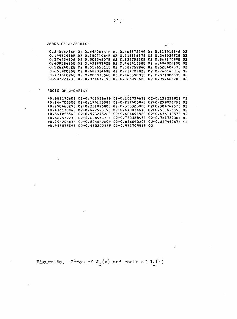
217

ZERCS OF J -ZERO(X)

c •24048256E 01 0 . 552C0781E 01 0 . 86537279E 01 0 . 11791534E 02 0 .1493C918E 02 0 . 18071C64E 02 0 . 2 1211637E 02 0 . 24352472E 02 0 .27493480E 02 0 . 3C634607E 02 C . 33775820E C2 O . 36917C99E 02 0 .40058426E 02 0 . 43199792E 02 0 . 46341188E 02 u . 49482610 E 02 0 .52624052E C 2 0 . 5576551 IE 02 0 . 589C6984E 02 0 . 62048469E 02 0 . 6519C035E 02 0 . 68331469E 02 0 . 7 1472982E C2 0 . 74614501E 02 0 . 77756026E 02 0 . 8C897556E 02 0 . 84C39091E C2 0 . 87180630E 02 0 . 90322173E 02 0 . 93463719E 02 0 . 96605268E 02 0 . 99746820E 02

ROOTS OF J -CNE(X)

+0 .38317060E 01*0 .70155367E 01+0 .10173463E +0 .164 7C630E 02+0 .19615858E 02+0 .2276C084E +0 .29C46829E 02+0 .32189680E 02+0 .35332308E +0 .41617094E 02+0 .44759319E 02+0 .47901461E +0 .54185554E 02+0 .57327526E C2+C.60469458E +0 .66753227E 02+0 .69895C72E 02+0 .73036895E +0 .7932C487E 02+0 .824È226CE 02+0 .8560402CE +0 .9 18 87 5C4É 02+0 .95029232E 02+0 .9817095 IE

02+0 .13323692E 02 C2+0 .259C3673E 02 C 2+0 . 384 74767E 02 02+0 .51043535E 02 02+0 .63611357E 02 C2+0 .76178700E 02 C2+0 .88745767E 02 02

Figure 46. Zeros of JQ(x) and roots of (x)