A Tensor Operations in Orthogonal Curvilinear Coordinate ...978-3-642-11594-3/1.pdf · A Tensor...

(A.1)

(A.2)

(A.3)

A Tensor Operations in Orthogonal CurvilinearCoordinate Systems

A.1 Change of Coordinate System

The vector and tensor operations we have discussed in the foregoing chapters wereperformed solely in rectangular coordinate system. It should be pointed out that wewere dealing with quantities such as velocity, acceleration, and pressure gradient thatare independent of any coordinate system within a certain frame of reference. In thisconnection it is necessary to distinguish between a coordinate system and a frame ofreference. The following example should clarify this distinction. In an absoluteframe of reference, the flow velocity vector may be described by the rectangularCartesian coordinate xi:

It may also be described by a cylindrical coordinate system, which is a non-Cartesiancoordinate system:

or generally by any other non-Cartesian or curvilinear coordinate i that describesthe flow channel geometry:

By changing the coordinate system, the flow velocity vector will not change. Itremains invariant under any transformation of coordinates. This is true for any otherquantities such as acceleration, force, pressure or temperature gradient. The conceptof invariance, however, is generally no longer valid if we change the frame ofreference. For example, if the flow particles leave the absolute frame of reference andenter the relative frame of reference, for example a moving or rotating frame, itsvelocity will experience a change. In this Chapter, we will pursue the concept ofquantity invariance and discuss the fundamentals that are needed for coordinatetransformation.

A.2 Co- and Contravariant Base Vectors, Metric Coefficients

As we saw in the previous chapter, a vector quantity is described in Cartesiancoordinate system xi by its components:

M.T. Schobeiri: Fluid Mechanics for Engineers, pp. 475–487. © Springer Berlin Heidelberg 2010

A Tensor Operations in Orthogonal Curvilinear Coordinate Systems476

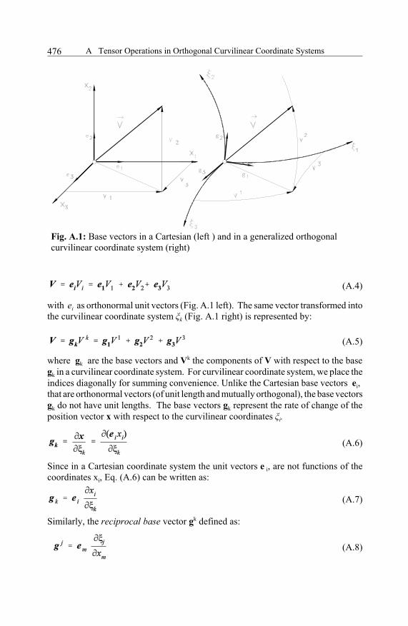
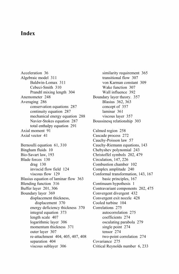
Fig. A.1: Base vectors in a Cartesian (left ) and in a generalized orthogonalcurvilinear coordinate system (right)

(A.4)

(A.5)

(A.6)

(A.7)

(A.8)

with ei as orthonormal unit vectors (Fig. A.1 left). The same vector transformed intothe curvilinear coordinate system k (Fig. A.1 right) is represented by:

where gk are the base vectors and Vk the components of V with respect to the basegk in a curvilinear coordinate system. For curvilinear coordinate system, we place theindices diagonally for summing convenience. Unlike the Cartesian base vectors ei,that are orthonormal vectors (of unit length and mutually orthogonal), the base vectorsgk do not have unit lengths. The base vectors gk represent the rate of change of theposition vector x with respect to the curvilinear coordinates i.

Since in a Cartesian coordinate system the unit vectors e i, are not functions of thecoordinates xi, Eq. (A.6) can be written as:

Similarly, the reciprocal base vector gk defined as:

A Tensor Operations in Orthogonal Curvilinear Coordinate Systems 477

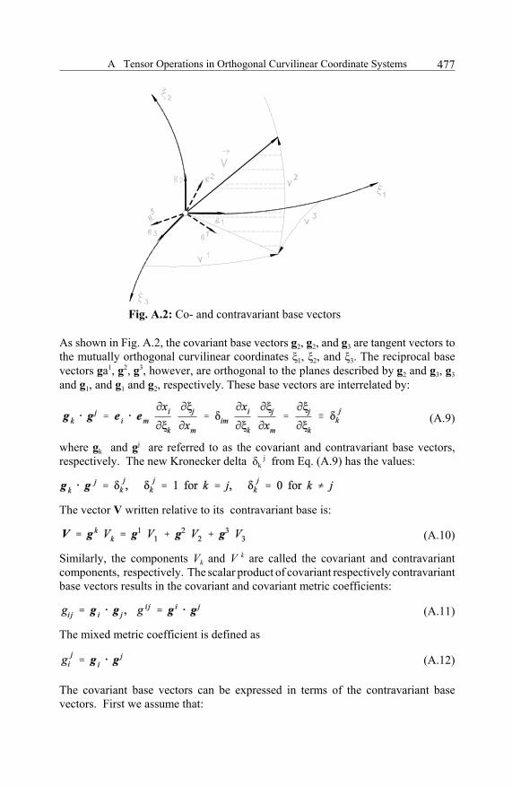
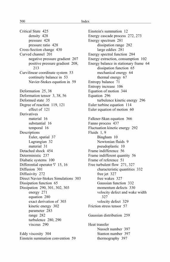
Fig. A.2: Co- and contravariant base vectors

(A.9)

(A.10)

(A.11)

(A.12)

As shown in Fig. A.2, the covariant base vectors g2, g2, and g3 are tangent vectors tothe mutually orthogonal curvilinear coordinates 1, 2, and 3. The reciprocal basevectors ga1, g2, g3, however, are orthogonal to the planes described by g2 and g3, g3and g1, and g1 and g2, respectively. These base vectors are interrelated by:

where gk and gj are referred to as the covariant and contravariant base vectors,respectively. The new Kronecker delta k

j from Eq. (A.9) has the values:

The vector V written relative to its contravariant base is:

Similarly, the components Vk and V k are called the covariant and contravariantcomponents, respectively. The scalar product of covariant respectively contravariantbase vectors results in the covariant and covariant metric coefficients:

The mixed metric coefficient is defined as

The covariant base vectors can be expressed in terms of the contravariant basevectors. First we assume that:


(A.13)

(A.14)

(A.16)

(A.17)

(A.18)

(A.19)

(A.20)

(A.21)

Generally the contravariant base vector can be written as

To find a direct relation between the base vectors, first the coefficient matrix Aij mustbe determined. To do so, we multiply Eq. (A.14) with gk scalarly:

This leads to . The right hand side is different from zero only if j = k.That means:

Introducing Eq. (A.16) into (A.14) results in a relation that expresses thecontravariant base vectors in terms of covariant base vectors:

The covariant base vector can also be expressed in terms of contravariant base vectorsin a similar way:

Multiply Eq. (A.l8) with (A.17) establishes a relationship between the covariant andcontravariant metric coefficients:

Applying the Kronecker delta on the right hand side results in:

A.3 Physical Components of a Vector

As mentioned previously, the base vectors gi or gj are not unit vectors.Consequently the co- and contravariant vector components Vj or V1 do not reflect thephysical components of vector V. To obtain the physical components, first thecorresponding unit vectors must be found. They can be obtained from:


(A.22)

(A.23)

(A.24)

(A.25)

(A.26)

(A.27)

(A.28a)

Similarly, the contravariant unit vectors are:

where gi* , represents the unit base vector, gi the absolute value of the base vector.

The expression (ii) denotes that no summing is carried out, whenever the indices areenclosed within parentheses. The vector can now be expressed in terms of its unitbase vectors and the corresponding physical components:

Thus the covariant and contravariant physical components can be easily obtainedfrom:

A.4 Derivatives of the Base Vectors, Christoffel Symbols

In a curvilinear coordinate system, the base vectors are generally functions of thecoordinates itself. This fact must be considered while differentiating the base vectors. Consider the derivative:

Similar to Eq. (A.7), the unit vector ek can be written:

Introducing Eq. (A.26) into (A.25) yields:

with ijn, and i jn as the Christoffel symbol of first and second kind, respectively

with the definition:


(A.30a)

(A.30b)

(A.31)

(A.32)

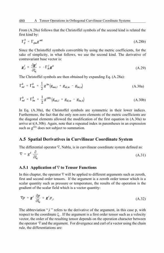
From (A.28a) follows that the Christoffel symbols of the second kind is related thefirst kind by:

Since the Christoffel symbols convertible by using the metric coefficients, for thesake of simplicity, in what follows, we use the second kind. The derivative ofcontravariant base vector is:

The Christoffel symbols are then obtained by expanding Eq. (A.28a):

In Eq. (A.30a), the Christoffel symbols are symmetric in their lower indices.Furthermore, the fact that the only non-zero elements of the metric coefficients arethe diagonal elements allowed the modification of the first equation in (A.30a) toarrive at t(A.30b). Again, note that a repeated index in parentheses in an expressionsuch as g(kk) does not subject to summation.

A.5 Spatial Derivatives in Curvilinear Coordinate System

The differential operator , Nabla, is in curvilinear coordinate system defined as:

A.5.1 Application of to Tensor Functions In this chapter, the operator will be applied to different arguments such as zeroth,first and second order tensors. If the argument is a zeroth order tensor which is ascalar quantity such as pressure or temperature, the results of the operation is thegradient of the scalar field which is a vector quantity:

The abbreviation “,i ” refers to the derivative of the argument, in this case p, withrespect to the coordinate i . If the argument is a first order tensor such as a velocityvector, the order of the resulting tensor depends on the operation character betweenthe operator and the argument. For divergence and curl of a vector using the chainrule, the differentiations are:

(A.29)

(A.28b)


(A.33a)

(A.33b)

(A.34a)

(A.34b)

(A.35)

(A.36)

(A.37)

(A.38)

(A.39)

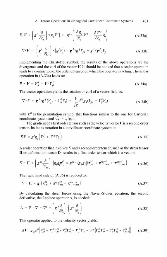
Implementing the Christoffel symbol, the results of the above operations are thedivergence and the curl of the vector V. It should be noticed that a scalar operationleads to a contraction of the order of tensor on which the operator is acting. The scalaroperation in (A.33a) leads to:

The vector operation yields the rotation or curl of a vector field as:

with as the permutation symbol that functions similar to the one for Cartesiancoordinate system and .

The gradient of a first order tensor such as the velocity vector V is a second ordertensor. Its index notation in a curvilinear coordinate system is:

A scalar operation that involves and a second order tensor, such as the stress tensor or deformation tensor D, results in a first order tensor which is a vector:

The right hand side of (A.36) is reduced to:

By calculating the shear forces using the Navier-Stokes equation, the secondderivative, the Laplace operator , is needed:

This operator applied to the velocity vector yields:


(A.40)

(A.41)

(A.42)

(A.43)

(A.44)

(A.45)

(A.46)

(A.47)

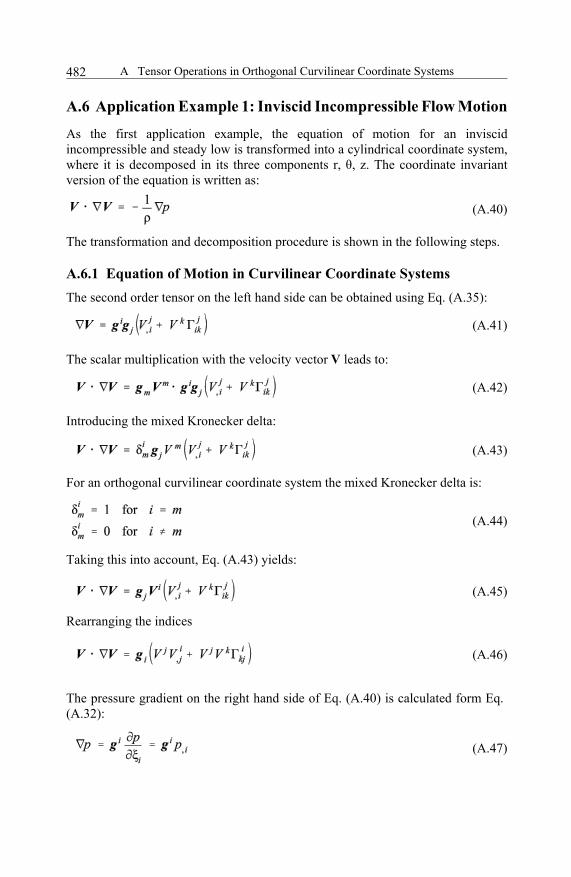
A.6 Application Example 1: Inviscid Incompressible Flow Motion

As the first application example, the equation of motion for an inviscidincompressible and steady low is transformed into a cylindrical coordinate system,where it is decomposed in its three components r, , z. The coordinate invariantversion of the equation is written as:

The transformation and decomposition procedure is shown in the following steps.

A.6.1 Equation of Motion in Curvilinear Coordinate SystemsThe second order tensor on the left hand side can be obtained using Eq. (A.35):

The scalar multiplication with the velocity vector V leads to:

Introducing the mixed Kronecker delta:

For an orthogonal curvilinear coordinate system the mixed Kronecker delta is:

Taking this into account, Eq. (A.43) yields:

Rearranging the indices

The pressure gradient on the right hand side of Eq. (A.40) is calculated form Eq. (A.32):


(A.48)

(A.49)

(A.50)

(A.51)

(A.52)

(A.53)

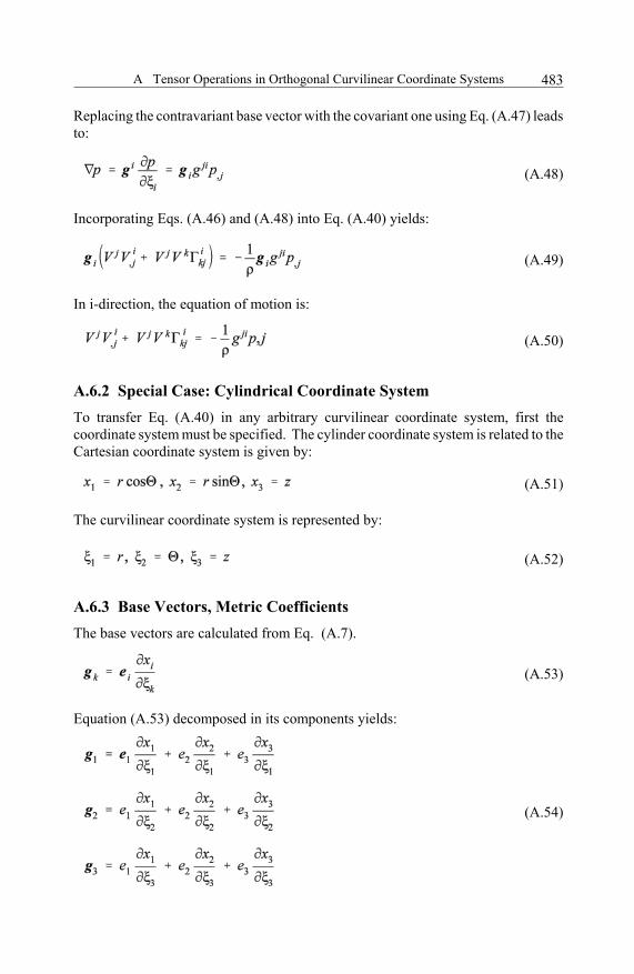
Replacing the contravariant base vector with the covariant one using Eq. (A.47) leadsto:

Incorporating Eqs. (A.46) and (A.48) into Eq. (A.40) yields:

In i-direction, the equation of motion is:

A.6.2 Special Case: Cylindrical Coordinate SystemTo transfer Eq. (A.40) in any arbitrary curvilinear coordinate system, first thecoordinate system must be specified. The cylinder coordinate system is related to theCartesian coordinate system is given by:

The curvilinear coordinate system is represented by:

A.6.3 Base Vectors, Metric CoefficientsThe base vectors are calculated from Eq. (A.7).

Equation (A.53) decomposed in its components yields:

(A.54)


(A.55)

(A.59)

(A.56)

(A.57a)

(A.57b)

(A.58)

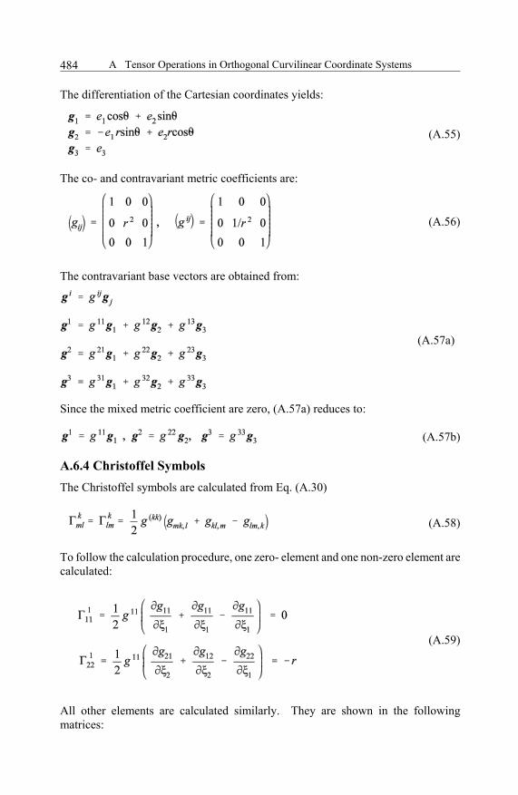
The differentiation of the Cartesian coordinates yields:

The co- and contravariant metric coefficients are:

The contravariant base vectors are obtained from:

Since the mixed metric coefficient are zero, (A.57a) reduces to:

A.6.4 Christoffel SymbolsThe Christoffel symbols are calculated from Eq. (A.30)

To follow the calculation procedure, one zero- element and one non-zero element arecalculated:

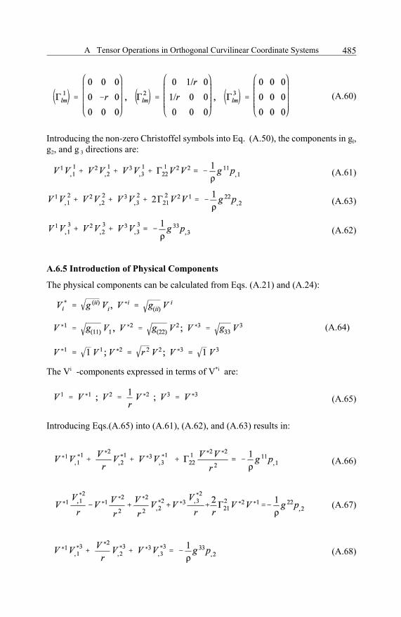
All other elements are calculated similarly. They are shown in the followingmatrices:


(A.60)

(A.61)

(A.62)

(A.63)

(A.64)

(A.65)

(A.66)

(A.67)

Introducing the non-zero Christoffel symbols into Eq. (A.50), the components in gl,g2, and g 3 directions are:

A.6.5 Introduction of Physical Components

The physical components can be calculated from Eqs. (A.21) and (A.24):

The Vi -components expressed in terms of V*i are:

Introducing Eqs.(A.65) into (A.61), (A.62), and (A.63) results in:

(A.68)


(A.69)

(A.73)

(A.70)

(A.71)

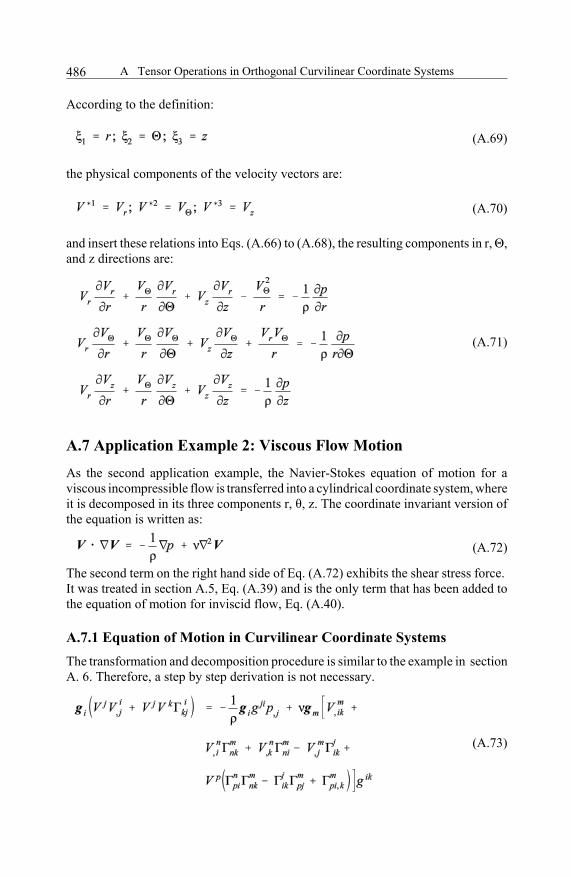
According to the definition:

the physical components of the velocity vectors are:

and insert these relations into Eqs. (A.66) to (A.68), the resulting components in r, ,and z directions are:

A.7 Application Example 2: Viscous Flow Motion

As the second application example, the Navier-Stokes equation of motion for aviscous incompressible flow is transferred into a cylindrical coordinate system, whereit is decomposed in its three components r, , z. The coordinate invariant version ofthe equation is written as:

The second term on the right hand side of Eq. (A.72) exhibits the shear stress force. It was treated in section A.5, Eq. (A.39) and is the only term that has been added tothe equation of motion for inviscid flow, Eq. (A.40).

A.7.1 Equation of Motion in Curvilinear Coordinate SystemsThe transformation and decomposition procedure is similar to the example in sectionA. 6. Therefore, a step by step derivation is not necessary.

(A.72)


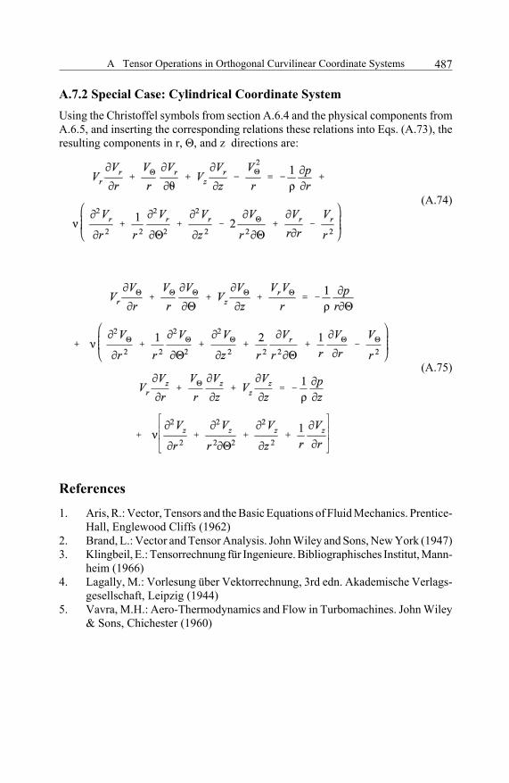
(A.74)

(A.75)

A.7.2 Special Case: Cylindrical Coordinate SystemUsing the Christoffel symbols from section A.6.4 and the physical components fromA.6.5, and inserting the corresponding relations these relations into Eqs. (A.73), theresulting components in r, , and z directions are:

References

1. Aris, R.: Vector, Tensors and the Basic Equations of Fluid Mechanics. Prentice-Hall, Englewood Cliffs (1962)

2. Brand, L.: Vector and Tensor Analysis. John Wiley and Sons, New York (1947)3. Klingbeil, E.: Tensorrechnung für Ingenieure. Bibliographisches Institut, Mann-

heim (1966)4. Lagally, M.: Vorlesung über Vektorrechnung, 3rd edn. Akademische Verlags-

gesellschaft, Leipzig (1944)5. Vavra, M.H.: Aero-Thermodynamics and Flow in Turbomachines. John Wiley

& Sons, Chichester (1960)

B Physical Properties of Dry Air

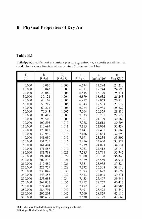
Table B.1

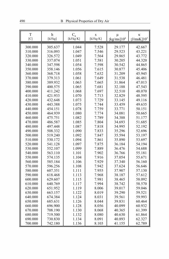
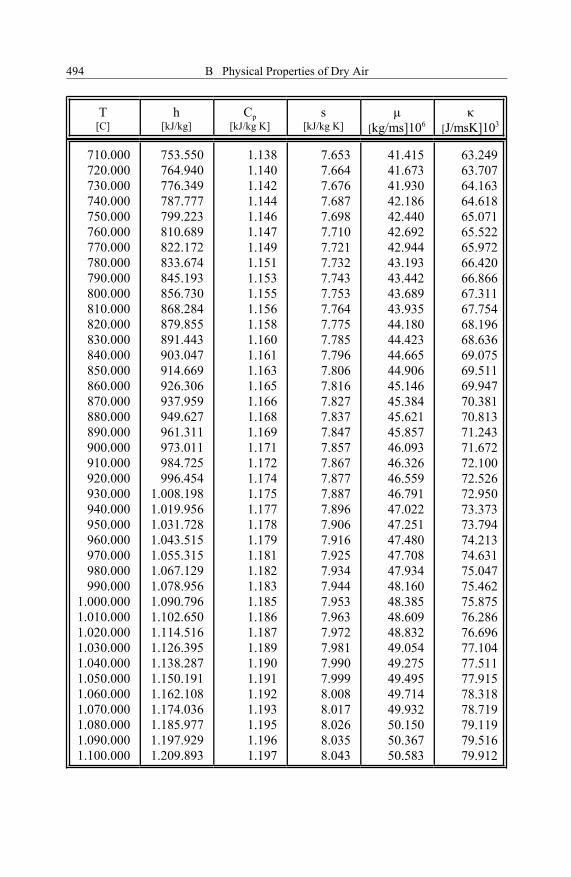
Enthalpy h, specific heat at constant pressure cp, entropy s, viscosity and thermalconductivity as a function of temperature T pressure p = 1 bar.

T[C]

h[kJ/kg]

Cp[kJ/kg K]

s[kJ/kg K] [kg/ms]106 [J/msK]103

0.00010.00020.00030.00040.00050.00060.00070.00080.00090.000

100.000110.000120.000130.000140.000150.000160.000170.000180.000190.000200.000210.000220.000230.000240.000250.000260.000270.000280.000290.000300.000

0.01010.04320.08030.12140.16750.21960.27770.34380.41790.500

100.593110.697120.812130.940141.080151.235161.404171.588181.788192.004202.238212.489222.759233.047243.355253.683264.032274.401284.791295.203305.637

1.0031.0031.0041.0041.0051.0051.0061.0071.0081.0091.0101.0111.0121.0131.0151.0161.0181.0191.0211.0221.0241.0261.0281.0301.0321.0341.0361.0381.0401.0421.044

6.7746.8116.8456.8796.9126.9436.9747.0047.0337.0617.0887.1157.1417.1667.1917.2167.2397.2637.2857.3087.3297.3517.3727.3937.4137.4337.4527.4727.4917.5097.528

17.29417.74418.19018.63219.06919.50319.93320.35920.78121.19921.61322.02422.43122.83423.23423.63024.02324.41224.79825.18025.55925.93526.30826.67727.04327.40727.76728.12428.47828.82929.177

24.21024.89325.57126.24326.91027.57228.22928.88029.52730.16930.80631.43932.06732.69033.30933.92434.53435.14035.74236.34036.93437.52438.11038.69239.27139.84640.41740.98541.54942.11042.667

M.T. Schobeiri: Fluid Mechanics for Engineers, pp. 489–497. © Springer Berlin Heidelberg 2010

B Physical Properties of Dry Air490

T[C]

h[kJ/kg]

Cp[kJ/kg K]


300.000310.000320.000330.000340.000350.000360.000370.000380.000390.000400.000410.000420.000430.000440.000450.000460.000470.000480.000490.000500.000510.000520.000530.000540.000550.000560.000570.000580.000590.000600.000610.000620.000630.000640.000650.000660.000670.000680.000690.000700.000

305.637316.093326.572337.074347.598358.146368.718379.313389.932400.575411.242421.933432.648443.388454.151464.939475.751486.587497.448508.332519.240530.172541.128552.107563.110574.135585.184596.256607.351618.468629.607640.769651.952663.157674.384685.631696.900708.190719.500730.830742.180

1.0441.0471.0491.0511.0541.0561.0581.0611.0631.0651.0681.0701.0731.0751.0781.0801.0821.0851.0871.0901.0921.0941.0971.0991.1011.1041.1061.1081.1111.1131.1151.1171.1191.1221.1241.1261.1281.1301.1321.1341.136

7.5287.5467.5647.5817.5987.6157.6327.6497.6657.6817.6977.7137.7297.7447.7597.7747.7897.8047.8187.8337.8477.8617.8757.8897.9027.9167.9297.9427.9557.9687.9817.9948.0068.0198.0318.0448.0568.0688.0808.0918.103

29.17729.52329.86530.20530.54230.87731.20931.53831.86432.18832.51032.82933.14533.45933.77134.08134.38834.69334.99535.29635.59435.89036.18436.47636.76637.05437.34037.62437.90738.18738.46538.74239.01739.29039.56139.83140.09940.36540.63040.89341.155

42.66743.22143.77244.32044.86545.40645.94546.48147.01347.54348.07048.59549.11649.63550.15150.66551.17751.68552.19252.69653.19753.69754.19454.68855.18155.67156.16056.64657.13057.61258.09258.57059.04659.52159.99360.46460.93261.39961.86462.32762.789

B Physical Properties of Dry Air 491

T[C]

h[kJ/kg]

Cp[kJ/kg K]


710.000720.000730.000740.000750.000760.000770.000780.000790.000800.000810.000820.000830.000840.000850.000860.000870.000880.000890.000900.000910.000920.000930.000940.000950.000960.000970.000980.000990.000

1.000.0001.010.0001.020.0001.030.0001.040.0001.050.0001.060.0001.070.0001.080.0001.090.0001.100.000

753.550764.940776.349787.777799.223810.689822.172833.674845.193856.730868.284879.855891.443903.047914.669926.306937.959949.627961.311973.011984.725996.454

1.008.1981.019.9561.031.7281.043.5151.055.3151.067.1291.078.9561.090.7961.102.6501.114.5161.126.3951.138.2871.150.1911.162.1081.174.0361.185.9771.197.9291.209.893

1.1381.1401.1421.1441.1461.1471.1491.1511.1531.1551.1561.1581.1601.1611.1631.1651.1661.1681.1691.1711.1721.1741.1751.1771.1781.1791.1811.1821.1831.1851.1861.1871.1891.1901.1911.1921.1931.1951.1961.197

8.1158.1268.1388.1498.1608.1728.1838.1948.2048.2158.2268.2378.2478.2588.2688.2788.2898.2998.3098.3198.3298.3398.3488.3588.3688.3778.3878.3968.4068.4158.4248.4348.4438.4528.4618.4708.4798.4888.4968.505

41.41541.67341.93042.18642.44042.69242.94443.19343.44243.68943.93544.18044.42344.66544.90645.14645.38445.62145.85746.09346.32646.55946.79147.02247.25147.48047.70847.93448.16048.38548.60948.83249.05449.27549.49549.71449.93250.15050.36750.583

63.24963.70764.16364.61865.07165.52265.97266.42066.86667.31167.75468.19668.63669.07569.51169.94770.38170.81371.24371.67272.10072.52672.95073.37373.79474.21374.63175.04775.46275.87576.28676.69677.10477.51177.91578.31878.71979.11979.51679.912


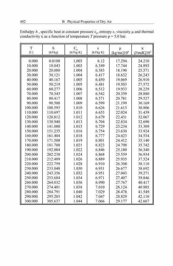
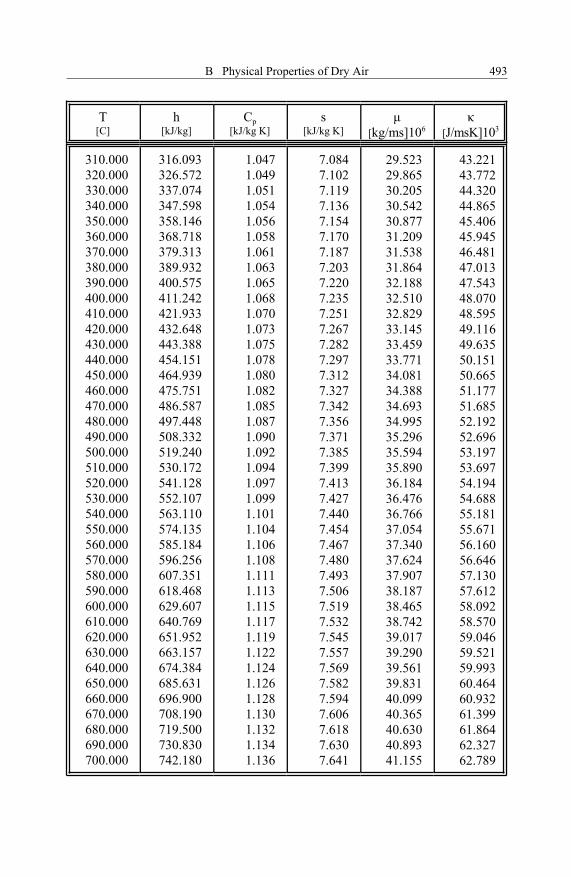
Enthalpy h , specific heat at constant pressure cp, entropy s, viscosity and thermalconductivity as a function of temperature T pressure p = 5.0 bar.

T[C]

h[kJ/kg]

Cp[kJ/kg K]


0.00010.00020.00030.00040.00050.00060.00070.00080.00090.000

100.000110.000120.000130.000140.000150.000160.000170.000180.000190.000200.000210.000220.000230.000240.000250.000260.000270.000280.000290.000300.000

0.010010.04320.08030.12140.16750.21960.27770.34380.41790.500

100.593110.697120.812130.940141.080151.235161.404171.588181.788192.004202.238212.489222.759233.048243.356253.684264.032274.401284.791295.203305.637

1,0031.0031.0041.0041.0051.0051.0061.0071.0081.0091.0101.0111.0121.0131.0151.0161.0181.0191.0211.0221.0241.0261.0281.0301.0321.0341.0361.0381.0401.0421.044

6.126.3496.3836.4176.4506.4816.5126.5426.5716.5996.6266.6536.6796.7046.7296.7546.7776.8016.8236.8466.8686.8896.9106.9316.9516.9716.9907.0107.0297.0477.066

17.29417.74418.19018.63219.06919.50319.93320.35920.78121.19921.61322.02422.43122.83423.23423.63024.02324.41224.79825.18025.55925.93526.30826.67727.04327.40727.76728.12428.47828.82929.177

24.21024.89325.57126.24326.91027.57228.22928.88029.52730.16930.80631.43932.06732.69033.30933.92434.53435.14035.74236.34036.93437.52438.11038.69239.27139.84640.41740.98541.54942.11042.667


T[C]

h[kJ/kg]

Cp[kJ/kg K]


310.000320.000330.000340.000350.000360.000370.000380.000390.000400.000410.000420.000430.000440.000450.000460.000470.000480.000490.000500.000510.000520.000530.000540.000550.000560.000570.000580.000590.000600.000610.000620.000630.000640.000650.000660.000670.000680.000690.000700.000

316.093326.572337.074347.598358.146368.718379.313389.932400.575411.242421.933432.648443.388454.151464.939475.751486.587497.448508.332519.240530.172541.128552.107563.110574.135585.184596.256607.351618.468629.607640.769651.952663.157674.384685.631696.900708.190719.500730.830742.180

1.0471.0491.0511.0541.0561.0581.0611.0631.0651.0681.0701.0731.0751.0781.0801.0821.0851.0871.0901.0921.0941.0971.0991.1011.1041.1061.1081.1111.1131.1151.1171.1191.1221.1241.1261.1281.1301.1321.1341.136

7.0847.1027.1197.1367.1547.1707.1877.2037.2207.2357.2517.2677.2827.2977.3127.3277.3427.3567.3717.3857.3997.4137.4277.4407.4547.4677.4807.4937.5067.5197.5327.5457.5577.5697.5827.5947.6067.6187.6307.641

29.52329.86530.20530.54230.87731.20931.53831.86432.18832.51032.82933.14533.45933.77134.08134.38834.69334.99535.29635.59435.89036.18436.47636.76637.05437.34037.62437.90738.18738.46538.74239.01739.29039.56139.83140.09940.36540.63040.89341.155

43.22143.77244.32044.86545.40645.94546.48147.01347.54348.07048.59549.11649.63550.15150.66551.17751.68552.19252.69653.19753.69754.19454.68855.18155.67156.16056.64657.13057.61258.09258.57059.04659.52159.99360.46460.93261.39961.86462.32762.789


T[C]

h[kJ/kg]

Cp[kJ/kg K]


710.000720.000730.000740.000750.000760.000770.000780.000790.000800.000810.000820.000830.000840.000850.000860.000870.000880.000890.000900.000910.000920.000930.000940.000950.000960.000970.000980.000990.000

1.000.0001.010.0001.020.0001.030.0001.040.0001.050.0001.060.0001.070.0001.080.0001.090.0001.100.000

753.550764.940776.349787.777799.223810.689822.172833.674845.193856.730868.284879.855891.443903.047914.669926.306937.959949.627961.311973.011984.725996.454

1.008.1981.019.9561.031.7281.043.5151.055.3151.067.1291.078.9561.090.7961.102.6501.114.5161.126.3951.138.2871.150.1911.162.1081.174.0361.185.9771.197.9291.209.893

1.1381.1401.1421.1441.1461.1471.1491.1511.1531.1551.1561.1581.1601.1611.1631.1651.1661.1681.1691.1711.1721.1741.1751.1771.1781.1791.1811.1821.1831.1851.1861.1871.1891.1901.1911.1921.1931.1951.1961.197

7.6537.6647.6767.6877.6987.7107.7217.7327.7437.7537.7647.7757.7857.7967.8067.8167.8277.8377.8477.8577.8677.8777.8877.8967.9067.9167.9257.9347.9447.9537.9637.9727.9817.9907.9998.0088.0178.0268.0358.043

41.41541.67341.93042.18642.44042.69242.94443.19343.44243.68943.93544.18044.42344.66544.90645.14645.38445.62145.85746.09346.32646.55946.79147.02247.25147.48047.70847.93448.16048.38548.60948.83249.05449.27549.49549.71449.93250.15050.36750.583

63.24963.70764.16364.61865.07165.52265.97266.42066.86667.31167.75468.19668.63669.07569.51169.94770.38170.81371.24371.67272.10072.52672.95073.37373.79474.21374.63175.04775.46275.87576.28676.69677.10477.51177.91578.31878.71979.11979.51679.912


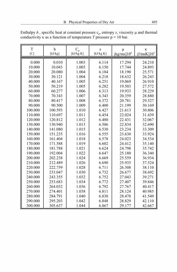
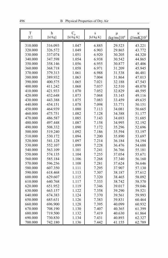
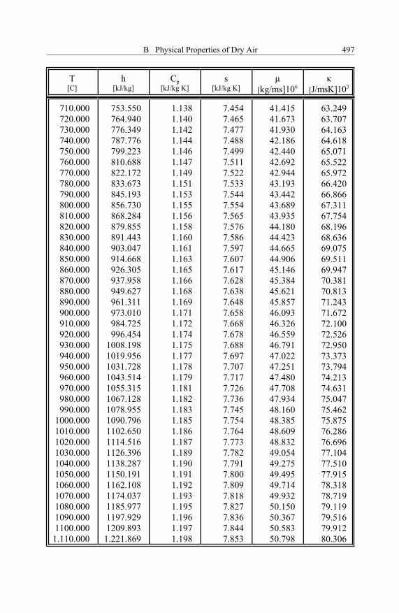
Enthalpy h , specific heat at constant pressure cp, entropy s, viscosity and thermalconductivity as a function of temperature T pressure p = 10 bar.

T[C]

h[kJ/kg]

Cp[kJ/kg K]


0.00010.00020.00030.00040.00050.00060.00070.00080.00090.000

100.000110.000120.000130.000140.000150.000160.000170.000180.000190.000200.000210.000220.000230.000240.000250.000260.000270.000280.000290.000300.000

0.01010.04320.08030.12140.16750.21960.27770.34380.41790.500

100.593110.697120.812130.940141.080151.235161.404171.588181.788192.004202.238212.489222.759233.047243.355253.683264.032274.401284.791295.203305.637

1.0031.0031.0041.0041.0051.0051.0061.0071.0081.0091.0101.0111.0121.0131.0151.0161.0181.0191.0211.0221.0241.0261.0281.0301.0321.0341.0361.0381.0401.0421.044

6.1146.1506.1846.2186.2516.2826.3136.3436.3726.4006.4276.4546.4806.5066.5306.5556.5786.6026.6246.6476.6696.6906.7116.7326.7526.7726.7926.8116.8306.8486.867

17.29417.74418.19018.63219.06919.50319.93320.35920.78121.19921.61322.02422.43122.83423.23423.63024.02324.41224.79825.18025.55925.93526.30826.67727.04327.40727.76728.12428.47828.82929.177

24.21024.89325.57126.24326.91027.57228.22928.88029.52730.16930.80631.43932.06732.69033.30933.92434.53435.14035.74236.34036.93437.52438.11038.69239.27139.84640.41740.98541.54942.11042.667


T[C]

h[kJ/kg]

Cp[kJ/kg K]


310.000320.000330.000340.000350.000360.000370.000380.000390.000400.000410.000420.000430.000440.000450.000460.000470.000480.000490.000500.000510.000520.000530.000540.000550.000560.000570.000580.000590.000600.000610.000620.000630.000640.000650.000660.000670.000680.000690.000700.000

316.093326.572337.074347.598358.146368.718379.313389.932400.575411.242421.933432.648443.388454.151464.939475.751486.587497.448508.332519.240530.172541.128552.107563.109574.135585.184596.256607.350618.468629.607640.768651.952663.157674.383685.631696.900708.190719.500730.830742.180

1.0471.0491.0511.0541.0561.0581.0611.0631.0651.0681.0701.0731.0751.0781.0801.0821.0851.0871.0901.0921.0941.0971.0991.1011.1041.1061.1081.1111.1131.1151.1171.1191.1221.1241.1261.1281.1301.1321.1341.136

6.8856.9036.9206.9386.9556.9716.9887.0047.0217.0377.0527.0687.0837.0987.1137.1287.1437.1587.1727.1867.2007.2147.2287.2417.2557.2687.2817.2957.3077.3207.3337.3467.3587.3707.3837.3957.4077.4197.4317.442

29.52329.86530.20530.54230.87731.20931.53831.86432.18832.51032.82933.14533.45933.77134.08134.38834.69334.99535.29635.59435.89036.18436.47636.76637.05437.34037.62437.90738.18738.46538.74239.01739.29039.56139.83140.09940.36540.63040.89341.155

43.22143.77244.32044.86545.40645.94546.48147.01347.54348.07048.59549.11649.63550.15150.66551.17751.68552.19252.69653.19753.69754.19454.68855.18155.67156.16056.64657.13057.61258.09258.57059.04659.52159.99360.46460.93261.39961.86462.32762.789


T[C]

h[kJ/kg]

Cp[kJ/kg K]


710.000720.000730.000740.000750.000760.000770.000780.000790.000800.000810.000820.000830.000840.000850.000860.000870.000880.000890.000900.000910.000920.000930.000940.000950.000960.000970.000980.000990.000

1000.0001010.0001020.0001030.0001040.0001050.0001060.0001070.0001080.0001090.0001100.000

1.110.000

753.550764.940776.349787.776799.223810.688822.172833.673845.193856.730868.284879.855891.443903.047914.668926.305937.958949.627961.311973.010984.725996.454

1008.1981019.9561031.7281043.5141055.3151067.1281078.9551090.7961102.6501114.5161126.3961138.2871150.1911162.1081174.0371185.9771197.9291209.893

1.221.869

1.1381.1401.1421.1441.1461.1471.1491.1511.1531.1551.1561.1581.1601.1611.1631.1651.1661.1681.1691.1711.1721.1741.1751.1771.1781.1791.1811.1821.1831.1851.1861.1871.1891.1901.1911.1921.1931.1951.1961.1971.198

7.4547.4657.4777.4887.4997.5117.5227.5337.5447.5547.5657.5767.5867.5977.6077.6177.6287.6387.6487.6587.6687.6787.6887.6977.7077.7177.7267.7367.7457.7547.7647.7737.7827.7917.8007.8097.8187.8277.8367.8447.853

41.41541.67341.93042.18642.44042.69242.94443.19343.44243.68943.93544.18044.42344.66544.90645.14645.38445.62145.85746.09346.32646.55946.79147.02247.25147.48047.70847.93448.16048.38548.60948.83249.05449.27549.49549.71449.93250.15050.36750.58350.798

63.24963.70764.16364.61865.07165.52265.97266.42066.86667.31167.75468.19668.63669.07569.51169.94770.38170.81371.24371.67272.10072.52672.95073.37373.79474.21374.63175.04775.46275.87576.28676.69677.10477.51077.91578.31878.71979.11979.51679.91280.306

Index

Acceleration 36Algebraic model 311

Baldwin-Lomax 311Cebeci-Smith 310Prandtl mixing length 304

Anemometer 248Averaging 286

conservation equations 287continuity equation 287mechanical energy equation 288Navier-Stokes equation 287total enthalpy equation 291

Axial moment 91Axial vector 41

Bernoulli equation 61, 310Bingham fluids 10Bio-Savart law, 193Blade forces 130

drag 130inviscid flow field 124viscous flow 129

Blasius equation of laminar flow 363Blending function 316Buffer layer 201, 306Boundary layer 369

displacement thickness,displacement 370

energy deficiency thickness 370integral equation 373length scale 407logarithmic layer 306momentum thickness 371outer layer 307re-attachment 404, 405, 407, 408separation 404viscous sublayer 306

similarity requirement 365transitional flow 307von Karman constant 309Wake function 307Wall influence 392

Boundary layer theory. 357Blasius 362, 363concept of 357laminar 361viscous layer 357

Boussinesq relationship 303

Calmed region 258Cascade process 272Cauchy-Poisson law 57Cauchy-Riemann equations, 143Chebyshev polynomial 243Christoffel symbols 202, 479Circulation, 147, 226Combustion chamber 102Complex amplitude 240Conformal transformation, 143, 167

basic principles, 167Continuum hypothesis 1Contravariant components 202, 475Convergent divergent 432Convergent exit nozzle 428Cooled turbine 104Correlations 275

autocorrelation 275coefficients 274osculating parabola 279single point 274tensor 274two-point correlation 274

Covariance 275Critical Reynolds number 6, 233

Index500

Critical State 425density 428pressure 428pressure ratio 428

Cross-Section change 430Curved channel 201

negative pressure gradient 207positive pressure gradient 208,

213Curvilinear coordinate system 53

continuity balance in 53Navier-Stokes equation in 59

Deformation 25, 38Deformation tensor 3, 38, 56Deformed state 35Degree of reaction 119, 121

effect of 121Derivatives

material 16substantial 16temporal 16

DescriptionsEuler, spatial 37Lagrangian 32material 31

Detached shock 454Deterministic 237Diabatic systems 100Differential operator 15, 16Diffusion 301Diffusivity 272Direct Navier-Stokes Simulations 303Dissipation function 65Dissipation 290, 301, 302, 303

energy 271equation 280exact derivation of 303kinetic energy 302parameter 283range 282turbulence 280, 290viscous 290

Eddy viscosity 304Einstein summation convention 59

Einstein's summation 12Energy cascade process 272, 273Energy spectrum 281

dissipation range 282large eddies 281

Energy spectral function 284Energy extraction, consumption 102Energy balance in stationary frame 64

dissipation function 65mechanical energy 64thermal energy 67

Entropy balance 71Entropy increase 106Equation of motion 344Equation 296

turbulence kinetic energy 296Euler turbine equation 114Euler equation of motion 60

Falkner-Skan equation 366Fanno process 437Fluctuation kinetic energy 292Fluids 1, 9

Bingham 10Newtonian fluids 9pseudoplastic 10

Frame indifference 56Frame indifferent quantity 56Frame of reference 51Free turbulent flow 271, 327

characteristic quantities 332free jet 327free wakes 327Gaussian function 332momentum defects 330velocity defect and wake width

327velocity defect 329

Friction stress tensor 57

Gaussian distribution 259

Heat transferNusselt number 397Stanton number 397thermography 397

Index 501

Helmholtzfirst theorem, 186second theorem, 186third theorem, 186

Holomorphic 143Homogeneous 1

gases 1liquids 1saturated 1superheated vapors 1unsaturated 1

Hot wire anemometry 391aliasing effect 393analog/digital converter 394constant current mode 391constant-temperature mode 391cross-wire 391folding frequency 394Nyquist-frequency 394sample frequency 393sampling rate 393signal conditioner 394single, cross and three-wire

probes 391single wire 391three-wire 391

Hugoniot relation 446Hypothesis

frozen turbulence 277G.I. Taylor 277Kolmogorov 272mixing length hypothesis 306

Incompressible 8, 202, 203, 210, 229Incompressibility condition 53Index notation 12Induced drag 195Induced velocity 190Integral balances

balance of energy 94balance of linear momentum 83balance of moment of momentum

88mass flow balance 81

Intermittency factor 6Intermittency function 390

Intermittency 6, 258averaged 259ensemble-averaged 259function 390maximum 259minimum 259

Inviscid 4, 208, 226, 227Inviscid flows, 139Irreversibility 106Irrotational flow 161, 140Irrotational 227, 228Isotropic turbulence 286Isotropy 273

Jacobianfunctional determinant 35transformation 32, 95

Joukowskiairfoil 172base profiles 172lift equation 163, 165transformation 169-171theorem 157

Kinetic energy 282, 285, 286, 292Kolmogorov 272

eddies 272first hypothesis 282hypothesis 272inertial subrange 281, 282length scale 281scales 281second hypothesis 283time scale 281universal equilibrium 272velocity scale 281

Kronecker tensor 57Kutta condition, 175Kutta-Joukowski

lift equation 163, 165transformation 169-171base profiles 172theorem 157

Laminar flow 4, 201Laminar flow stability 233

Index502

Laminar boundary layer 362Blasius equation 363Faulkner-Skan equation 366Hartree 366Polhausen approximate 367

Laminar-turbulent transition 234Laplace equation 144Laurent series 163Laval nozzle 431Lift coefficient 128Linear wall function 306

Mach number 423, 425Magnus effect 159Mass flow function 429Material acceleration 18Material derivative 32Mean free path 1Metric coefficients 203Mixing length hypothesis 304Momentum balance frame 53

Natural transition 236Navier-Stokes 295

equation 273, 274, 278, 287, 295, 296operator 295

Navier-Stokes equation 205for compressible fluids 58solution of 205Direct Navier Stokes DNS 303

Neutral stability 242Newtonian fluids 9, 57Normal shock 445Nusselt number 397

Oblique shock 432, 451Orr-Sommerfeld

eigenvalue problem 241stability equation 239

Oscillation frequency 240Osculating parabola 279

Pathline, streamline, streakline 44Peclet number 388

effective 389turbulent 388

Physical component 203Pohlhausen 368

profiles 369slope of the velocity profiles 369velocity profiles 369

Potential function 160Potential flows 139, 140Power law 385Prandtl boundary layer

experimental observations 357mixing length 388mixing length hypothesis 306mixing length model 390power law 385theory 357, 362

Prandtl number 387, 388effective Prandtl number 390molecular Prandtl number 388,

390turbulent Prandtl number 388

Principle of material objectivity 56

Radial flow 209Radial equilibrium 117Rayleigh process 437Reaction force 87Residue theorem 164Reynolds number 234

critical 234subcritical 234supercritical 234

Reynolds transport theorem 42, 89Richardson energy cascade 273Riemann mapping theorem, 143Rotating frame 74,

continuity equation in 74energy equation in 77equation of motion in 75

Rotation 25, 38Rotation tensor 56Rotational flow 218, 227, 228

Index 503

Scalar product of 19Scales of turbulence 273

length of the smallest eddy 273time scale 272, 273, 274

Separation 208, 209, 214, 215Shaft power 97Shear stress momenta 90Shear viscosity 58Similarity condition 365Small disturbance 237solution 364Spatial differential 16Spatial change 16Spatially periodic velocity distribution

255Specific total energy 95Specific lift force 159Spectral tensor 284Speed of sound 423Stable laminar flow 242Stage load coefficient 121Stagnation point 426Stanton number 397Stationary frame 51Statistically steady flow 237Steady flow 9Stream function 154Stress tensor 56

apparent 273Structure 1Substantial change 16Superposition principle 217Superposition of potential flows 150

complex potential 150Dipole 151Dipole and a vortex 154translational flow 151uniform flow, source, and sink

159Supersonic diffuser 432Supersonic flow 450

Taylor 279eddies 277frozen turbulence 277hypothesis 277

micro length scale 279time scale 279

Temporal change 16Tensor 11, 294

contraction 11, 15deformation 299eigenvalue 25eigenvector 25 first order 11friction stress 289product 13, 14Reynolds stress 294rotation 311second order 11zeroth-order 11

Tensor product of and V 21, 29Thermal turbomachinery stages 110Tollmien-Schlichting waves. 6, 236Total momentum 331Total pressure loss 106Transformation vector function 33Transition 260

bypass transition 237natural 260wake induced 260

Transitional region 6Translation 38Turbine 104

cooled 104uncooled 103

Turbo-shafts 102Turbochargers 110Turbomachinery stages

dimensionless parameters 115energy transfer in 110flow deflection 114flow forces 124

Turbulence 273anisotropic 281convective diffusion 301correlations 274diffusion 272free turbulence 271homogeneous 273isotropic 273, 282isotropy 273

Index504

kinetic energy 297length and time scales 273, 304production 301type of 271, 273viscous dissipation 301viscous diffusion 272wall turbulence 271

Turbulence model 271, 304algebraic model 304Baldwin-Lomax model 311Cebeci-Smith model 310One-Equation model 312Prandtl mixing length 304standard k- vs. k- 318two-equation k- model 313two-equation k- -model 315two-equation SST-model 316

Turbulent kinetic energy 297Turbulent flow, fully developed 307Types of free turbulent flows 327

Uncooled turbine 103Universal equilibrium 272Unsteady flow 9

ensemble averaging 9Unsteady boundary layer 409

Strouhal number 398wake generator 398

Unsteady compressible flow 458

Variation of length scale 407pressure gradient 408

Vector product 21

Vector 11cross product 13scalar product 13tensor product 14

Velocity 2, 36Velocity diagram 104Velocity gradient 38Velocity fluctuations 331Velocity momenta 86Velocity potential, 141Velocity scales 304Velocity spectrum 284Viscous sublayer 306Viscous diffusion 272Viscous 201, 202, 205, 208, 216, 226,

227Von Kármán constant 309Von Kármán 373

integral equation 373Vortex line 185Vortex filament 185Vortex 225-227, 273Vortex theorems

Helmholtz theorems 185Thomson 179

Vorticity 21Vorticity vector 40

Wake 327free wakes 328velocity defect 327width 327

Wavenumber space 284, 285Wavenumber vector 284Wavenumber 285

A Tensor Operations in Orthogonal Curvilinear Coordinate ...978-3-642-11594-3/1.pdf · A Tensor...

Documents

Transcript of A Tensor Operations in Orthogonal Curvilinear Coordinate ...978-3-642-11594-3/1.pdf · A Tensor...