A Tail-Index Analysis of Stochastic Gradient Noise in Deep Neural Networks

Umut Simsekli 1 Levent Sagun 2 Mert Gurbuzbalaban 3

AbstractThe gradient noise (GN) in the stochastic gra-dient descent (SGD) algorithm is often consid-ered to be Gaussian in the large data regime byassuming that the classical central limit theo-rem (CLT) kicks in. This assumption is oftenmade for mathematical convenience, since it en-ables SGD to be analyzed as a stochastic differ-ential equation (SDE) driven by a Brownian mo-tion. We argue that the Gaussianity assumptionmight fail to hold in deep learning settings andhence render the Brownian motion-based analy-ses inappropriate. Inspired by non-Gaussian nat-ural phenomena, we consider the GN in a moregeneral context and invoke the generalized CLT(GCLT), which suggests that the GN convergesto a heavy-tailed α-stable random variable. Ac-cordingly, we propose to analyze SGD as an SDEdriven by a Levy motion. Such SDEs can in-cur ‘jumps’, which force the SDE transition fromnarrow minima to wider minima, as proven byexisting metastability theory. To validate the α-stable assumption, we conduct experiments oncommon deep learning scenarios and show thatin all settings, the GN is highly non-Gaussian andadmits heavy-tails. We investigate the tail behav-ior in varying network architectures and sizes,loss functions, and datasets. Our results open upa different perspective and shed more light on thebelief that SGD prefers wide minima.

1. IntroductionContext and motivation: Deep neural networks have rev-olutionized machine learning and have ubiquitous use in

1LTCI, Telecom ParisTech, Universite Paris-Saclay, 75013,Paris, France 2Institute of Physics, Ecole Polytechnique Federalede Lausanne, 1015 Lausanne, Switzerland 3Department of Man-agement Science and Information Systems, Rutgers BusinessSchool, NJ 08854, USA. Correspondence to: Umut Simsekli<umut.simsekli@telecom-paristech.fr>.

Proceedings of the 36 th International Conference on MachineLearning, Long Beach, California, PMLR 97, 2019. Copyright2019 by the author(s).

many application domains (LeCun et al., 2015; Krizhevskyet al., 2012; Hinton et al., 2012). In full generality, manykey tasks in deep learning reduces to solving the followingoptimization problem:

w? = arg minw∈Rp

f(w) ,

1

n

∑n

i=1f (i)(w)

(1)

where w ∈ Rp denotes the weights of the neural net-work, f : Rp → R denotes the loss function that is typ-ically non-convex in w, each f (i) denotes the (instanta-neous) loss function that is contributed by the data pointi ∈ 1, . . . , n, and n denotes the total number of datapoints. Stochastic gradient descent (SGD) is one the mostpopular approaches for attacking this problem in practiceand is based on the following iterative updates:

wk+1 = wk − η∇fk(wk) (2)

where k ∈ 1, . . . ,K denotes the iteration number, η isthe step-size, and ∇fk denotes the stochastic gradient atiteration k, that is defined as follows:

∇fk(w) , ∇fΩk(w) ,1

b

∑i∈Ωk

∇f (i)(w). (3)

Here, Ωk ⊂ 1, . . . , n is a random subset that is drawnwith or without replacement at iteration k, and b = |Ωk|denotes the number of elements in Ωk.

SGD is widely used in deep learning with a great successin its computational efficiency (Bottou, 2010; Bottou &Bousquet, 2008; Daneshmand et al., 2018). Beyond effi-ciency, understanding how SGD performs better than itsfull batch counterpart in terms of test accuracy remains amajor challenge. Even though SGD seems to find zeroloss solutions on the training landscape (at least in certainregimes (Zhang et al., 2017a; Sagun et al., 2015; Keskaret al., 2016; Geiger et al., 2018)), it appears that the al-gorithm finds solutions with different properties dependingon how it is tuned (Sutskever et al., 2013; Keskar et al.,2016; Jastrzebski et al., 2017; Hoffer et al., 2017; Masters& Luschi, 2018; Smith et al., 2017). Despite the fact thatthe impact of SGD on generalization has been studied (Ad-vani & Saxe, 2017; Wu et al., 2018; Neyshabur et al., 2017),a satisfactory theory that can explain its success in a waythat encompasses such peculiar empirical properties is stilllacking.

A Tail Analysis of SGD in Deep Learning

A popular approach for investigating the behavior SGDis based on considering SGD as a discretization of acontinuous-time process (Mandt et al., 2016; Jastrzebskiet al., 2017; Li et al., 2017a; Hu et al., 2017; Zhu et al.,2018; Chaudhari & Soatto, 2018). This approach mainlyrequires the following assumption1 on the stochastic gradi-ent noise Uk(w) , ∇fk(w)−∇f(w):

Uk(w) ∼ N (0, σ2I), (4)

whereN denotes the multivariate (Gaussian) normal distri-bution and I denotes the identity matrix of appropriate size.The rationale behind this assumption is that, if the size ofthe minibatch b is large enough, then we can invoke theCentral Limit Theorem (CLT) and assume that the distri-bution of Uk is approximately Gaussian. Then, under thisassumption, (2) can be written as follows:

wk+1 = wk − η∇f(wk) +√η√ησ2Zk, (5)

where Zk denotes a standard normal random variable inRp. If we further assume that η is small enough, then thecontinuous-time analogue of the discrete-time process (5)is the following stochastic differential equation (SDE):2

dwt = −∇f(wt)dt+√ησ2dBt, (6)

where Bt denotes the standard Brownian motion. ThisSDE is a variant of the well-known Langevin diffusionand under mild regularity assumptions on f , one canshow that the Markov process (wt)t≥0 is ergodic with itsunique invariant measure, whose density is proportional toexp(−f(x)/(ησ2)) for any η > 0. (Roberts & Stramer,2002). From this perspective, the SGD recursion in (5) canbe seen as a first-order Euler-Maruyama discretization ofthe Langevin dynamics (see also (Li et al., 2017a; Jastrzeb-ski et al., 2017; Hu et al., 2017)), which is often referredto as the Unadjusted Langevin Algorithm (ULA) (Roberts& Stramer, 2002; Lamberton & Pages, 2003; Durmus &Moulines, 2015; Durmus et al., 2016).

Based on this observation, Jastrzebski et al. (2017) focusedon the relation between this invariant measure and the al-gorithm parameters, namely the step-size η and mini-batchsize, as a function of σ2. They concluded that the ratio oflearning rate divided by the batch size is the control pa-rameter that determines the width of the minima found by

1We note that more sophisticated assumptions than (4) havebeen made in terms of the covariance matrix of the Gaussian dis-tribution (e.g. state dependent, anisotropic). However, in all thesecases, the resulting distribution is still a Gaussian, therefore thesame criticism holds.

2 In a recent work with a similar critic taken on the recent the-ories on the SGD dynamics, some theoretical concerns have beenalso raised about the SDE approximation of SGD (Yaida, 2019).We believe that the SDE representation is sufficiently accurate forsmall step-sizes and a good, if not the best, proxy for understand-ing the behavior of SGD.

(a) Real (b) Gaussian (c) α-stable

Figure 1. (a)The histogram of the norm of the gradient noisescomputed with AlexNet on Cifar10. (b) and (c) the histograms ofthe norms of (scaled) Guassian and α-stable random variables.

SGD. Furthermore, they revisit the famous wide minimafolklore (Hochreiter & Schmidhuber, 1997): Among theminima found by SGD, the wider it is, the better it performson the test set. However, there are several fundamental is-sues with this approach, which we will explain below.

We first illustrate a typical mismatch between the Gaus-sianity assumption and the empirical behavior of thestochastic gradient noise. In Figure 1, we plot the his-togram of the norms of the stochastic gradient noise thatis computed using a convolutional neural network in a realclassification problem and compare it to the histogram ofthe norms of Gaussian random variables. It can be clearlyobserved that the shape of the real histogram is very differ-ent than the Gaussian and shows a heavy-tailed behavior.

In addition to the empirical observations, the Gaussianityassumption also yields some theoretical issues. The firstissue with this assumption is that the current SDE analy-ses of SGD are based on the invariant measure of the SDE,which implicitly assumes that sufficiently many iterationshave been taken to converge to that measure. Recent re-sults on ULA (Raginsky et al., 2017; Xu et al., 2018) haveshown that, the required number of iterations to achievethe invariant measure often grows exponentially with thedimension p. This result contradicts with the current prac-tice: considering the large size of the neural networks andlimited computational budget, only a limited number of it-erations – which is much smaller than exp(O(p)) – can betaken. This conflict becomes clearer in the light of the re-cent works that studied the local behavior of ULA (Tzenet al., 2018; Zhang et al., 2017b). These studies showedthat ULA will get close to the nearest local optimum inpolynomial time; however, the required amount of time forescaping from that local optimum increases exponentiallywith the dimension. Therefore, the phenomenon that SGDprefers wide minima within a considerably small numberof iterations cannot be explained using the asymptotic dis-tribution of the SDE given in (6).

The second issue is related to the local behavior of the pro-cess and becomes clear when we consider the metastabilityanalysis of Brownian motion-driven SDEs. These studies(Freidlin & Wentzell, 1998; Bovier et al., 2004; Imkeller

A Tail Analysis of SGD in Deep Learning

et al., 2010b) consider the case where w0 is initialized in aquadratic basin and then analyze the minimum time t suchthat wt is outside that basin. They show that this so-calledfirst exit time depends exponentially on the height of thebasin; however, this dependency is only polynomial withthe width of the basin. These theoretical results directlycontradict with the wide minima phenomenon: even if theheight of a basin is slightly larger, the exit-time from thisbasin will be dominated by its height, which implies thatthe process would stay longer in (or in other words, ‘pre-fer’) deeper minima as opposed to wider minima. The rea-son why the exit-time is dominated by the height is due tothe continuity of the Brownian motion, which is in fact adirect consequence of the Gaussian noise assumption.

A final remark on the issues of this approach is the ob-servation that landscape is flat at the bottom regardless ofthe batch size used in SGD (Sagun et al., 2017). In par-ticular, the spectrum of the Hessian at a near critical pointwith close to zero loss value has many near zero eigenval-ues. Therefore, local curvature measures that are used as aproxy for measuring the width of a basin correlates with themagnitudes of large eigenvalues of the Hessian which arefew. Besides, during the dynamics of SGD it has been ob-served that the algorithm does not cross barriers except per-haps at the very initial phase (Xing et al., 2018; Baity-Jesiet al., 2018). Such dependence of width on an essentially-flat landscape combined with the lack of explicit barriercrossing during the SGD descent forces us to rethink theanalysis of basin hopping under a noisy dynamics.

Proposed framework: In this study, we aim at addressingthese contradictions and come up with an arguably better-suited hypothesis for the stochastic gradient noise that hasmore pertinent theoretical implications for the phenomenaassociated with SGD. In particular, we go back to (3) and(4) and reconsider the application of CLT. This classicalCLT assumes that Uk is a sum of many independent andidentically distributed (i.i.d.) random variables, whose vari-ance is finite, and then it states that the law of Uk convergesto a Gaussian distribution, which then paves the way for(5). Even though the finite-variance assumption seems nat-ural and intuitive at the first sight, it turns out that in manydomains, such as turbulent motions (Weeks et al., 1995),oceanic fluid flows (Woyczynski, 2001), finance (Mandel-brot, 2013), biological evolution (Jourdain et al., 2012), au-dio signals (Liutkus & Badeau, 2015; Simsekli et al., 2015;Leglaive et al., 2017; Simsekli et al., 2018), brain signals(Jas et al., 2017), the assumption might fail to hold (see(Duan, 2015) for more examples). In such cases, the clas-sical CLT along with the Gaussian approximation will nolonger hold. While this might seem daunting, fortunately,one can prove an extended CLT and show that the law ofthe sum of these i.i.d. variables with infinite variance stillconverges to a family of heavy-tailed distributions that is

called the α-stable distribution (Levy, 1937). As we willdetail in Section 2, these distributions are parametrized bytheir tail-index α ∈ (0, 2] and they coincide with the Gaus-sian distribution when α = 2.

In this study, we relax the finite-variance assumption onthe stochastic gradient noise and by invoking the extendedCLT, we assume that Uk follows an α-stable distribution,as hinted in Figure 1(c). By following a similar ratio-nale to (5) and (6), we reformulate SGD with this new as-sumption and consider its continuous-time limit for smallstep-sizes. Since the noise might not be Gaussian anymore(i.e. when α 6= 2), the use of the Brownian motion wouldnot be appropriate in this case and we need to replace itwith the α-stable Levy motion, whose increments have anα-stable distribution (Yanovsky et al., 2000). Due to theheavy-tailed nature of α-stable distribution, the Levy mo-tion might incur large discontinuous jumps and thereforeexhibits a fundamentally different behavior than the Brow-nian motion, whose paths are on the contrary almost surelycontinuous. As we will describe in detail in Section 2,the discontinuities also reflect in the metastability proper-ties of Levy-driven SDEs, which indicate that, as soon asα < 2, the first exit time from a basin does not depend onits height; on the contrary, it directly depends on its widthand the tail-index α. Informally, this implies that the pro-cess will escape from narrow minima – no matter how deepthey are – and stay longer in wide minima. Besides, as αget smaller, the probability for the dynamics to jump in awide basin will increase. Therefore, if the α-stable assump-tion on the stochastic gradient noise holds, then the existingmetastability results automatically provide strong theoreti-cal insights for illuminating the behavior of SGD.

Contributions: The main contributions of this paper aretwofold: (i) we perform an extensive empirical analysis ofthe tail-index of the stochastic gradient noise in deep neuralnetworks and (ii) based on these empirical results, we bringan alternative perspective to the existing approaches for an-alyzing SGD and shed more light on the folklore that SGDprefers wide minima by establishing a bridge between SGDand the related theoretical results from statistical physicsand stochastic analysis.

We conduct experiments on the most common deep learn-ing architectures. In particular, we investigate the tail be-havior under fully-connected and convolutional models us-ing negative log likelihood and linear hinge loss functionson MNIST, CIFAR10, and CIFAR100 datasets. For eachconfiguration, we scale the size of the network and batchsize used in SGD and monitor the effect of each of thesesettings on the tail index α.

Our experiments reveal several remarkable results:

• In all our configurations, the stochastic gradient noise

A Tail Analysis of SGD in Deep Learning

-10 -5 0 5 1010

-4

10-3

10-2

10-1 =1.8

=2.0

0 1000 2000 3000-20

0

20

=1.8

=2.0

Figure 2. Left: SαS densities, right: Lαt for p = 1. For α < 2,SαS becomes heavier-tailed and Lαt incurs jumps.

turns out to be highly non-Gaussian and possesses aheavy-tailed behavior.

• Increasing the size of the minibatch has a very little im-pact on the tail-index, and as opposed to the commonbelief that larger minibatches result in Gaussian gradientnoise, the noise is still far from being Gaussian.

• There is a strong interaction between the network archi-tecture, network size, dataset, and the tail-index, whichultimately determine the dynamics of SGD on the train-ing surface. This observation supports the view that, thegeometry of the problem and the dynamics induced bythe algorithm cannot be separated from each other.

• In almost all configurations, we observe two distinctphases of SGD throughout iterations. During the firstphase, the tail-index rapidly decreases and SGD pos-sesses a clear jump when the tail-index is at its lowestvalue and causes a sudden jump in the accuracy. Thisbehavior strengthens the view that SGD crosses barriersat the very initial phase.

Our methodology also opens up several interesting futuredirections and open questions, as we discuss in Section 5.

2. Stable distributions and SGD as aLevy-Driven SDE

The CLT states that the sum of i.i.d. random variables witha finite second moment converges to a normal distributionif the number of summands grow. However, if the variableshave heavy-tail, the second moment may not exist. For in-stance, if their density p(x) has a power-law tail decreasingas 1/|x|α+1 where 0 < α < 2; only α-th moment existwith α < 2. In this case, generalized central limit theorem(GCLT) says that the sum of such variables will convergeto a distribution called the α-stable distribution instead asthe number of summands grows (see e.g. (Fischer, 2010).In this work, we focus on the centered symmetric α-stable(SαS) distribution, which is a special case of α-stable dis-tributions that are symmetric around the origin.

We can view the SαS distribution as a heavy-tailed gener-alization of a centered Gaussian distribution. The SαS dis-tributions are defined through their characteristic functionvia X ∼ SαS(σ) ⇐⇒ E[exp(iωX)] = exp(−|σω|α).Even though their probability density function does not

admit a closed-form formula in general except in spe-cial cases, their density decays with a power law tail like1/|x|α+1 where α ∈ (0, 2] is called the tail-index which de-termines the behavior of the distribution: as α gets smaller;the distribution has a heavier tail. In fact, the parameter αalso determines the moments: when α < 2, E[|X|r] < ∞if and only if r < α; implyingX has infinite variance whenα 6= 2. The parameter σ ∈ R+ is the scale parameter andcontrols the spread of X around 0. We recover the Gaus-sian distribution N (0, 2σ2) as a special case when α = 2.

In this study, we make the following assumption on thestochastic gradient noise:

[Uk(w)]i ∼ SαS(σ(w)), ∀i = 1, . . . , n (7)

where [v]i denotes the i’th component of a vector v. In-formally, we assume that each coordinate of Uk is SαSdistributed with the same α and the scale parameter σ de-pends on the state w. Here, this dependency is not crucialsince we are mainly interested in the tail-index α, whichcan be estimated independently from the scale parameter.Therefore, we will simply denote σ(w) as σ for clarity.

By using the assumption (7), we can rewrite the SGD re-cursion as follows (Simsekli, 2017; Nguyen et al., 2019):

wk+1 = wk − η∇f(wk) + η1/α(ηα−1α σ

)Sk, (8)

where Sk ∈ Rp is a random vector such that [Sk]i ∼SαS(1). If the step-size η is small enough, then we canconsider the continuous-time limit of this discrete-timeprocess, which is expressed in the following SDE drivenby an α-stable Levy process:

dwt = −∇f(wt)dt+ η(α−1)/ασ dLαt , (9)

where Lαt denotes the p-dimensional α-stable Levy motionwith independent components. In other words, each com-ponent of Lαt is an independent α-stable Levy motion in R.For the scalar case it is defined as follows for α ∈ (0, 2](Duan, 2015):

(i) Lα0 = 0 almost surely.

(ii) For t0 < t1 < · · · < tN , the increments (Lαti−Lαti−1)

are independent (i = 1, . . . , N ).

(iii) The difference (Lαt − Lαs ) and Lαt−s have the samedistribution: SαS((t− s)1/α) for s < t.

(iv) Lαt is continuous in probability (i.e. it has stochas-tically continuous sample paths): for all δ > 0 ands ≥ 0, p(|Lαt − Lαs | > δ)→ 0 as t→ s.

It is easy to check that the noise term in (8) is obtainedby integrating Lαt from kη to (k + 1)η. When α = 2, Lαtcoincides with a scaled version of Brownian motion,

√2Bt.

SαS and Lαt are illustrated in Figure 2.

A Tail Analysis of SGD in Deep Learning

The SDE in (9) exhibits a fundamentally different behaviorthan the one in (6) does. This is mostly due to the stochas-tic continuity property of Lαt , which enables Lαt to have acountable number of discontinuities, which are sometimescalled ‘jumps’. In the rest of this section, we will recall im-portant theoretical results about this SDE and discuss theirimplications on SGD.

For clarity of the presentation and notational simplicitywe focus on the scalar case and consider the SDE (9) inR (i.e. p = 1). Multidimensional generalizations of themetastability results presented in this paper can be found in(Imkeller et al., 2010a). We rewrite (9) as follows:

dwεt = −∇f(wεt )dt+ εdLαt (10)

for t ≥ 0, started from the initial point w0 ∈ R, where Lαtis the α-stable Levy process, ε ≥ 0 is a parameter and f isa non-convex objective with r ≥ 2 local minima.

When ε = 0, we recover the gradient descent dynamicsin continuous time: dw0

t = −∇f(w0t )dt, where the lo-

cal minima are the stable points of this differential equa-tion. However, as soon as ε > 0, these states become‘metastable’, meaning that there is a positive probabilityforwεt to transition from one basin to another. However, thetime required for transitioning to another basin strongly de-pends on the characteristics of the injected noise. The twomost important cases are α = 2 and α < 2. When α = 2,(i.e. the Gaussianity assumption) the process (wεt )t≥0 iscontinuous, which requires it to ‘climb’ the basin all theway up, in order to be able to transition to another basin.This fact makes the transition-time depend on the height ofthe basin. On the contrary, when α < 2, the process canincur discontinuities and do not need to cross the bound-aries of the basin in order to transition to another one sinceit can directly jump. This property is called the ‘transitionphenomenon’ (Duan, 2015) and makes the transition-timemostly depend on the width of the basin. In the rest of thesection, we will formalize these explanations.

Gradient-like flows driven by Brownian motion and weakerror for their discretization is well studied from a theoret-ical standpoint (see e.g. (Li et al., 2017b; Mertikopoulos &Staudigl, 2018)), however their Levy driven analogue (10)and the discrete-time versions (Burghoff & Pavlyukevich,2015) are relatively less studied. Under some assumptionson the objective f , it is known that the process (10) admits astationary density (Samorodnitsky & Grigoriu, 2003). Fora general f , an explicit formula for the equilibrium distribu-tion is not known, however when the noise level ε is smallenough, finer characterizations of the structure of the equi-librium density in dimension one is known. We next sum-marize known results in this area, which show that Levy-driven dynamics spends more time in ‘wide valleys’ in thesense of (Chaudhari et al., 2017) when ε goes to zero.

Assume that f is smooth with r local minima miri=1 sep-arated by r − 1 local maxima sir−1

i=1 , i.e.

−∞ := s0 < m1 < s1 < · · · < sr−1 < mr < sr :=∞.

Furthermore, assume that the local minima and maximaare not degenerate, i.e. f ′′(mi) > 0 and f ′′(si) < 0for every i. We also assume the objective gradient hasa growth condition f ′(w) > |w|1+c for some constantc > 0 and when |w| is large enough. Each local minimami lies in the (interval) valley Si = (si−1, si) of (width)length Li = |si − si−1|. Consider also a δ-neighborhoodBi := |x − mi| ≤ δ around the local minimum withδ > 0 small enough so that the neighborhood is containedin the valley Si for every i. We are interested in the firstexit time from Bi starting from a point w0 ∈ Bi and thetransition time T iw0

(ε) := inft ≥ 0 : wεt ∈ ∪j 6=iBj toa neighborhood of another local minimum, we will removethe dependency to w0 of the transition time in our discus-sions as it is clear from the context. The following resultshows that the transition times are asymptotically exponen-tially distributed in the limit of small noise and scales like1/εα with ε.Theorem 1 ((Pavlyukevich, 2007)). For an initial pointw0 ∈ Bi, in the limit ε→ 0, the following statements holdregarding the transition time:

Pw0(T i(ε) ∈ Bj) → qijq

−1i if i 6= j,

Pw0(εαT i(ε) ≥ u) ≤ e−qiu for any u ≥ 0.

where

qij =1

α

∣∣∣∣ 1

|sj−1 −mi|α− 1

|sj −mi|α

∣∣∣∣ , (11)

qi =∑j 6=i

qij . (12)

If the SDE (10) would be driven by the Brownian motioninstead, then an analogous theorem to Theorem 1 holdssaying that the transition times are still exponentially dis-tributed but the scaling εα needs to be replaced by e2H/ε2

where H is the maximal depth of the basins to be traversedbetween the two local minima (Day, 1983; Bovier et al.,2005). This means that in the small noise limit, Brownian-motion driven gradient descent dynamics need exponentialtime to transit to another minimum whereas Levy-drivengradient descent dynamics need only polynomial time. Wealso note from Theorem 1 that the mean transition time be-tween valleys for Levy SDE does not depend on the depthH of the valleys they reside in which is an advantage overBrownian motion driven SDE in the existence of deep val-leys. Informally, this difference is due to the fact that Brow-nian motion driven SDE has to typically climb up a valleyto exit it, whereas Levy-driven SDE could jump out.

The following theorem says that as ε → 0, up to a nor-malization in time, the process wεt behaves like a finite

A Tail Analysis of SGD in Deep Learning

state-space Markov process that has support over the setof local minima miri=1 admitting a stationary densityπ = (πi)

ri=1 with an infinitesimal generator Q. The pro-

cess jumps between the valleys Si, spending time propor-tional to probability pi amount of time in each valley in theequilibrium where the probabilities π = (πi)

ri=1 are given

by the solution to the linear system Qπ = 0.

Theorem 2 ((Pavlyukevich, 2007)). Let w0 ∈ Si, for some1 ≤ i ≤ r. For t ≥ 0, wεtε−α → Ym(t), as ε → 0, inthe sense of finite-dimensional distributions, where Y =(Ym(t))t≥0 is a continuous-time Markov chain on a statespace m1,m2, . . . ,mr with the infinitesimal generatorQ = (qij)

ri,j=1 with

qij =1

α

∣∣∣∣ 1

|sj−1 −mi|α− 1

|sj −mi|α

∣∣∣∣ , (13)

qii = −∑

j 6=iqij . (14)

This process admits a density π satisfying QTπ = 0.

A consequence of this theorem is that equilibrium proba-bilities pi are typically larger for “wide valleys”. To seethis consider the special case illustrated in Figure 3(a) withr = 2 local minima m1 < s1 = 0 < m2 separated by alocal maximum at s1 = 0. For this example, m2 > |m1|,and the second local minimum lies in a wider valley. Asimple computation reveals π1 = |m1|α/(|m1|α + mα

2 ),π2 = |m2|α/(|m1|α + |m2|α).

We see that π2 > π1, that is in the equilibrium the processspends more time on the wider valley. In particular, the

ratio π2

π1=(m2

|m1|

)αgrows with an exponent α when the

ratio m2

|m1| of the width of the valleys grows. Consequently,if the gradient noise is indeed α-stable distributed, theseresults directly provide theoretical evidence for the wide-minima behavior of SGD.

3. Experimental Setup and MethodologyExperimental setup: We investigate the tail behaviorof the stochastic gradient noise in a variety of scenarios.We first consider a fully-connected network (FCN) on theMNIST and CIFAR10 datasets. For this model, we vary thedepth (i.e. the number of layers) in the set 2, 3, . . . , 10,the width (i.e. the number of neurons per layer) in the set2, 4, 8, . . . , 1024, and the minibatch size ranging from 1to full batch. We then consider a convolutional neural net-work (CNN) architecture (AlexNet) on the CIFAR10 andCIFAR100 datasets. We scale the number of filters in eachconvolutional layer in range 2, 4, . . . , 512. We randomlysplit the MNIST dataset into train and test parts of sizes60K and 10K, and CIFAR10 and CIFAR100 datasets intotrain and test parts of sizes 50K and 10K, respectively. The

(a) (b)

Figure 3. (a) An objective with two local minima m1,m2 seper-ated by a local maxima at s1 = 0. (b) Illustration of the tail-indexestimator α.

order of the total number of parameters p range from sev-eral thousands to tens of millions.

For both fully connected and convolutional settings, we runeach configuration with the negative-log-likelihood (i.e.cross entropy) and with the linear hinge loss, and we re-peat each experiment with three different random seeds.The training algorithm is SGD with no explicit modifi-cation such as momentum or weight decay. The train-ing runs until 100% training accuracy is achieved or un-til maximum number of iterations limit is reached (thelatter limit is effective in the under-parametrized mod-els). At every 100th iteration, we log the full train-ing and test accuracies, and the tail estimate of the gra-dients that are sampled using the corresponding mini-batch size. The codebase is implemented in python us-ing pytorch and provided in https://github.com/umutsimsekli/sgd_tail_index. Total runtime is∼3 weeks on 8 relatively modern GPUs.

Method for tail-index estimation: Estimating the tail-index of an extreme-value distribution is a long-standingtopic. Some of the well-known estimators for this task are(Hill, 1975; Pickands, 1975; Dekkers et al., 1989; De Haan& Peng, 1998). Despite their popularity, these methods arenot specifically developed for α-stable distributions and ithas been shown that they might fail for estimating the tail-index for α-stable distributions (Mittnik & Rachev, 1996;Paulauskas & Vaiciulis, 2011).

In this study, we use a relatively recent estimator proposedin (Mohammadi et al., 2015) for α-stable distributions. Itis given in the following theorem.

Theorem 3 (Mohammadi et al. (2015)). Let XiKi=1 bea collection of random variables with Xi ∼ SαS(σ) andK = K1 × K2. Define Yi ,

∑K1

j=1Xj+(i−1)K1for i ∈

J1,K2K. Then, the estimator

1

α,

1

logK1

( 1

K2

K2∑i=1

log |Yi| −1

K

K∑i=1

log |Xi|). (15)

converges to 1/α almost surely, as K2 →∞.

A Tail Analysis of SGD in Deep Learning

As shown in Theorem 2.3 of (Mohammadi et al., 2015),this estimator admits a faster convergence rate and smallerasymptotic variance than all the aforementioned methods.

In order to verify the accuracy of this estimator, we conducta preliminary experiment, where we first generate K =K1 ×K2 many SαS(1) distributed random variables withK1 = 100,K2 = 1000 for 100 different values of α. Then,we estimate α by using α , ( 1

α )−1. We repeat thisexperiment 100 times for each α. As shown in Figure 3(b),the estimator is very accurate for a large range of α. Due toits favorable theoretical properties such as independence ofthe scale parameter σ, combined with its empirical stability,we choose this estimator in our experiments.

In order to estimate the tail-index α at iteration k, we firstpartition the set of data points D , 1, . . . , n into manydisjoint sets Ωik ⊂ D of size b, such that the union ofthese subsets give all the data points. Formally, for alli, j = 1, . . . , n/b, |Ωik| = b, ∪iΩik = D, and Ωik ∩ Ωjk = ∅for i 6= j. This approach is similar to sampling withoutreplacement. We then compute the full gradient ∇f(wk)and the stochastic gradients∇fΩik

(wk) for each minibatchΩik. We finally compute the stochastic gradient noisesU ik(wk) = ∇fΩik

(wk)−∇f(wk), vectorize each U ik(wk)and concatenate them to obtain a single vector, and com-pute the reciprocal of (15). In this case, we haveK = pn/band we setK1 to the divisor ofK that is the closest to

√K.

4. ResultsIn this section we present the most important and represen-tative results. We have observed that, in all configurations,the choice of the two loss functions and the three differentinitializations yield no significant difference. Therefore,throughout this section, we will focus on the negative-log-likelihood loss. Unless stated otherwise, we set the mini-batch size b = 500 and the step-size η = 0.1.

Effect of varying network size: In our first set of experi-ments, we measure the tail-index for varying the widths anddepths for the FCN, and varying widths (i.e. the number offilters) for the CNN. For very small sizes, the networks per-form poorly, therefore, we only illustrate sufficiently largenetwork sizes, which yield similar accuracies. For these ex-periments, we compute the average of the tail-index mea-surements for the last 10K iterations (i.e. when α becomesstationary) to focus on the late stage dynamics.

Figure 4 shows the results for the FCN. The first strikingobservation is that in all the cases, the estimated tail-indexis far from 2 with a very high confidence (the variance ofthe estimates were around 0.001), meaning that the distri-bution of the gradient noise is highly non-Gaussian. For theMNIST dataset, we observe that α systematically decreases

(a) MNIST

(b) CIFAR10

Figure 4. Estimation of α for varying widths and depths in FCN.The curves in the left figures correspond to different depths, andthe ones on the right figures correspond to widths.

(a) CIFAR10

(b) CIFAR100

Figure 5. The accuracy and α of the CNN for varying widths.

for increasing network size, where this behavior becomesmore prominent with the depth. This result shows that, forMNIST, increasing the dimension of the network results ina gradient noise with heavier tails and therefore increasesthe probability to end up in a wider basin.

For the CIFAR10 dataset, we still observe that α is far from2; however, in this case, increasing the network size doesnot have a clear effect on α: in all cases, we observe that αis in the range 1.1–1.2.

Figure 5 shows the results for the CNN. In this figure, wealso depict the train and test accuracy, as well as the tail-index that is estimated on the test set. These results show

A Tail Analysis of SGD in Deep Learning

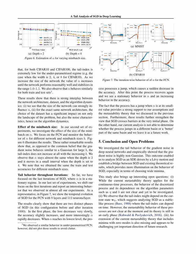
(a) Depth = 2 (b) Depth = 4

Figure 6. Estimation of α for varying minibatch size.

that, for both CIFAR10 and CIFAR100, the tail-index isextremely low for the under-parametrized regime (e.g. thecase when the width is 2, 4, or 8 for CIFAR10). As weincrease the size of the network the value of α increasesuntil the network performs reasonably well and stabilizes inthe range 1.0–1.1. We also observe that α behaves similarlyfor both train and test sets3.

These results show that there is strong interplay betweenthe network architecture, dataset, and the algorithm dynam-ics: (i) we see that the size of the network can strongly in-fluence α, (ii) for the exact same network architecture, thechoice of the dataset has a significant impact on not onlythe landscape of the problem, but also the noise character-istics, hence on the algorithm dynamics.

Effect of the minibatch size: In our second set of ex-periments, we investigate the effect of the size of the mini-batch on α. We focus on the FCN and monitor the behav-ior of α for different network and minibatch sizes b. Fig-ure 6 illustrates the results. These rather remarkable resultsshow that, as opposed to the common belief that the gra-dient noise behaves similar to a Gaussian for large b, thetail-index does not increase at all with the increasing b. Weobserve that α stays almost the same when the depth is 2and it moves in a small interval when the depth is set to4. We note that we obtained the same the train and testaccuracies for different minibatch sizes.

Tail behavior throughout iterations: So far, we havefocused on the last iterations of SGD, where α is in a sta-tionary regime. In our last set of experiments, we shift ourfocus on the first iterations and report an interesting behav-ior that we observed in almost all our experiments. As arepresentative, in Figure 7, we show the temporal evolutionof SGD for the FCN with 9 layers and 512 neurons/layer.

The results clearly show that there are two distinct phasesof SGD (in this configuration before and after iteration1000). In the first phase, the loss decreases very slowly,the accuracy slightly increases, and more interestingly αrapidly decreases. When α reaches its lowest level, the pro-

3We observed a similar behavior in under-parametrized FCN;however, did not plot those results to avoid clutter.

(a) MNIST

(b) CIFAR10

Figure 7. The iteration-wise behavior of of α for the FCN.

cess possesses a jump, which causes a sudden decrease inthe accuracy. After this point the process recovers againand we see a stationary behavior in α and an increasingbehavior in the accuracy.

The fact that the process has a jump when α is at its small-est value provides a strong support to our assumptions andthe metastability theory that we discussed in the previoussection. Furthermore, these results further strengthen theview that SGD crosses barriers at the very initial phase. Onthe other hand, our current analysis is not able to determinewhether the process jumps in a different basin or a ‘better’part of the same basin and we leave it as a future work.

5. Conclusion and Open ProblemsWe investigated the tail behavior of the gradient noise indeep neural networks and empirically showed that the gra-dient noise is highly non-Gaussian. This outcome enabledus to analyze SGD as an SDE driven by a Levy motion andestablish a bridge between SGD and existing theoretical re-sults, which provides more illumination on the behavior ofSGD, especially in terms of choosing wide minima.

This study also brings up interesting open questions: (i)While the current metastability theory applies for thecontinuous-time processes, the behavior of the discretizedprocess and its dependence on the algorithm parameterssuch as η and b are not clear and yet to be investigated.(ii) We observe that the tail-index might depend on the cur-rent state wk, which suggests analyzing SGD as a stable-like process (Bass, 1988) where the tail-index can dependon time. However, the metastability behavior of these pro-cesses are not clear at the moment and its theory is still inan early phase (Kuhwald & Pavlyukevich, 2016). (iii) Anextension of the current metastability theory that includesminima with zero modes is also missing and appears to bechallenging yet important direction of future research.

A Tail Analysis of SGD in Deep Learning

AcknowledgmentsThis work is partly supported by the French NationalResearch Agency (ANR) as a part of the FBIMATRIXproject (ANR-16-CE23-0014). Mert Gurbuzbalaban ac-knowledges support from the grants NSF DMS-1723085and NSF CCF-1814888.

ReferencesAdvani, M. S. and Saxe, A. M. High-dimensional dynamics

of generalization error in neural networks. arXiv preprintarXiv:1710.03667, 2017.

Baity-Jesi, M., Sagun, L., Geiger, M., Spigler, S., Arous,G. B., Cammarota, C., LeCun, Y., Wyart, M., and Biroli,G. Comparing dynamics: Deep neural networks versusglassy systems. In International Conference on MachineLearning, volume 80, pp. 314–323, Stockholm Sweden,10–15 Jul 2018.

Bass, R. F. Uniqueness in law for pure jump Markov pro-cesses. Probability Theory and Related Fields, 79(2):271–287, 1988.

Bottou, L. Large-scale machine learning with stochasticgradient descent. In Proceedings of COMPSTAT’2010,pp. 177–186. Physica-Verlag HD, 2010.

Bottou, L. and Bousquet, O. The tradeoffs of large scalelearning. In Advances in Neural Information ProcessingSystems, pp. 161–168, 2008.

Bovier, A., Eckhoff, M., Gayrard, V., and Klein, M.Metastability in reversible diffusion processes i: Sharpasymptotics for capacities and exit times. Journal of theEuropean Mathematical Society, 6(4):399–424, 2004.

Bovier, A., Gayrard, V., and Klein, M. Metastability in re-versible diffusion processes ii: Precise asymptotics forsmall eigenvalues. Journal of the European Mathemati-cal Society, 7(1):69–99, 2005.

Burghoff, T. and Pavlyukevich, I. Spectral analysis for adiscrete metastable system driven by levy flights. Jour-nal of Statistical Physics, 161(1):171–196, 2015.

Chaudhari, P. and Soatto, S. Stochastic gradient descentperforms variational inference, converges to limit cy-cles for deep networks. In International Conference onLearning Representations, 2018.

Chaudhari, P., Choromanska, A., Soatto, S., LeCun, Y.,Baldassi, C., Borgs, C., Chayes, J., Sagun, L., andZecchina, R. Entropy-sgd: Biasing gradient descent intowide valleys. In International Conference on LearningRepresentations (ICLR), 2017.

Daneshmand, H., Kohler, J., Lucchi, A., and Hofmann, T.Escaping saddles with stochastic gradients. In ICML, pp.1155–1164, 2018.

Day, M. V. On the exponential exit law in the small param-eter exit problem. Stochastics, 8(4):297–323, 1983.

De Haan, L. and Peng, L. Comparison of tail index estima-tors. Statistica Neerlandica, 52(1):60–70, 1998.

Dekkers, A. L. M., Einmahl, J. H. J., and De Haan, L. Amoment estimator for the index of an extreme-value dis-tribution. The Annals of Statistics, pp. 1833–1855, 1989.

Duan, J. An Introduction to Stochastic Dynamics. Cam-bridge University Press, New York, 2015.

Durmus, A. and Moulines, E. Non-asymptotic convergenceanalysis for the unadjusted Langevin algorithm. arXivpreprint arXiv:1507.05021, 2015.

Durmus, A., Simsekli, U., Moulines, E., Badeau, R., andRichard, G. Stochastic gradient Richardson-RombergMarkov Chain Monte Carlo. In NIPS, 2016.

Fischer, H. A history of the central limit theorem: Fromclassical to modern probability theory. Springer Science& Business Media, 2010.

Freidlin, M. I. and Wentzell, A. D. Random perturbations.In Random perturbations of dynamical systems, pp. 15–43. Springer, 1998.

Geiger, M., Spigler, S., d’Ascoli, S., Sagun, L., Baity-Jesi,M., Biroli, G., and Wyart, M. The jamming transition asa paradigm to understand the loss landscape of deep neu-ral networks. arXiv preprint arXiv:1809.09349, 2018.

Hill, B. M. A simple general approach to inference aboutthe tail of a distribution. The Annals of Statistics, pp.1163–1174, 1975.

Hinton, G., Deng, L., Yu, D., Dahl, G. E., Mohamed, A.-r., Jaitly, N., Senior, A., Vanhoucke, V., Nguyen, P.,Sainath, T. N., et al. Deep neural networks for acous-tic modeling in speech recognition: The shared views offour research groups. IEEE Signal processing magazine,29(6):82–97, 2012.

Hochreiter, S. and Schmidhuber, J. Flat minima. NeuralComputation, 9(1):1–42, 1997.

Hoffer, E., Hubara, I., and Soudry, D. Train longer, gener-alize better: closing the generalization gap in large batchtraining of neural networks. In Advances in Neural In-formation Processing Systems, pp. 1731–1741, 2017.

Hu, W., Li, C. J., Li, L., and Liu, J.-G. On the diffusionapproximation of nonconvex stochastic gradient descent.arXiv preprint arXiv:1705.07562, 2017.

A Tail Analysis of SGD in Deep Learning

Imkeller, P., Pavlyukevich, I., and Stauch, M. First exittimes of non-linear dynamical systems in rd perturbed bymultifractal Levy noise. Journal of Statistical Physics,141(1):94–119, 2010a.

Imkeller, P., Pavlyukevich, I., and Wetzel, T. The hierarchyof exit times of Levy-driven Langevin equations. TheEuropean Physical Journal Special Topics, 191(1):211–222, Dec 2010b.

Jas, M., Dupre La Tour, T., Simsekli, U., and Gramfort,A. Learning the morphology of brain signals usingalpha-stable convolutional sparse coding. In Advances inNeural Information Processing Systems, pp. 1099–1108,2017.

Jastrzebski, S., Kenton, Z., Arpit, D., Ballas, N., Fischer,A., Bengio, Y., and Storkey, A. Three factors influencingminima in sgd. arXiv preprint arXiv:1711.04623, 2017.

Jourdain, B., Meleard, S., and Woyczynski, W. A. Levyflights in evolutionary ecology. Journal of MathematicalBiology, 65(4):677–707, 2012.

Keskar, N. S., Mudigere, D., Nocedal, J., Smelyanskiy,M., and Tang, P. T. P. On large-batch training for deeplearning: Generalization gap and sharp minima. arXivpreprint arXiv:1609.04836, 2016.

Krizhevsky, A., Sutskever, I., and Hinton, G. E. Imagenetclassification with deep convolutional neural networks.In Advances in Neural Information Processing Systems,pp. 1097–1105, 2012.

Kuhwald, I. and Pavlyukevich, I. Bistable behaviour of ajump-diffusion driven by a periodic stable-like additiveprocess. Discrete & Continuous Dynamical Systems-Series B, 21(9), 2016.

Lamberton, D. and Pages, G. Recursive computation of theinvariant distribution of a diffusion: the case of a weaklymean reverting drift. Stochastics and dynamics, 3(04):435–451, 2003.

LeCun, Y., Bengio, Y., and Hinton, G. Deep learning. Na-ture, 521:436 EP –, 05 2015. URL https://doi.org/10.1038/nature14539.

Leglaive, S., Simsekli, U., Liutkus, A., Badeau, R., andRichard, G. Alpha-stable multichannel audio sourceseparation. In 2017 IEEE International Conference onAcoustics, Speech and Signal Processing (ICASSP), pp.576–580. IEEE, 2017.

Levy, P. Theorie de l’addition des variables aleatoires.Gauthiers-Villars, Paris, 1937.

Li, Q., Tai, C., and E, W. Stochastic modified equationsand adaptive stochastic gradient algorithms. In Proceed-ings of the 34th International Conference on MachineLearning, pp. 2101–2110, 06–11 Aug 2017a.

Li, Q., Tai, C., and Weinan, E. Stochastic modified equa-tions and adaptive stochastic gradient algorithms. In In-ternational Conference on Machine Learning, pp. 2101–2110, 2017b.

Liutkus, A. and Badeau, R. Generalized Wiener filteringwith fractional power spectrograms. In IEEE Interna-tional Conference on Acoustics, Speech and Signal Pro-cessing (ICASSP), pp. 266–270. IEEE, 2015.

Mandelbrot, B. B. Fractals and Scaling in Finance:Discontinuity, Concentration, Risk. Selecta Volume E.Springer Science & Business Media, 2013.

Mandt, S., Hoffman, M., and Blei, D. A variational anal-ysis of stochastic gradient algorithms. In InternationalConference on Machine Learning, pp. 354–363, 2016.

Masters, D. and Luschi, C. Revisiting small batchtraining for deep neural networks. arXiv preprintarXiv:1804.07612, 2018.

Mertikopoulos, P. and Staudigl, M. On the convergenceof gradient-like flows with noisy gradient input. SIAMJournal on Optimization, 28(1):163–197, 2018.

Mittnik, S. and Rachev, S. T. Tail estimation of the sta-ble index α. Applied Mathematics Letters, 9(3):53–56,1996.

Mohammadi, M., Mohammadpour, A., and Ogata, H. Onestimating the tail index and the spectral measure of mul-tivariate α-stable distributions. Metrika, 78(5):549–561,2015.

Neyshabur, B., Bhojanapalli, S., McAllester, D., and Sre-bro, N. Exploring generalization in deep learning. InAdvances in Neural Information Processing Systems, pp.5947–5956, 2017.

Nguyen, T. H., Simsekli, U., , and Richard, G. Non-asymptotic analysis of fractional Langevin Monte Carlofor non-convex optimization. In ICML, 2019.

Paulauskas, V. and Vaiciulis, M. Once more on comparisonof tail index estimators. arXiv preprint arXiv:1104.1242,2011.

Pavlyukevich, I. Cooling down levy flights. Journalof Physics A: Mathematical and Theoretical, 40(41):12299, 2007.

Pickands, J. Statistical inference using extreme order statis-tics. The Annals of Statistics, 3(1):119–131, 1975.

A Tail Analysis of SGD in Deep Learning

Raginsky, M., Rakhlin, A., and Telgarsky, M. Non-convexlearning via stochastic gradient Langevin dynamics: anonasymptotic analysis. In Proceedings of the 2017Conference on Learning Theory, volume 65, pp. 1674–1703, 2017.

Roberts, G. O. and Stramer, O. Langevin Diffusionsand Metropolis-Hastings Algorithms. Methodology andComputing in Applied Probability, 4(4):337–357, De-cember 2002. ISSN 13875841.

Sagun, L., Guney, V. U., Ben Arous, G., and LeCun, Y.Explorations on high dimensional landscapes. Interna-tional Conference on Learning Representations Work-shop Contribution, arXiv:1412.6615, 2015.

Sagun, L., Evci, U., Guney, V. U., Dauphin, Y., andBottou, L. Empirical analysis of the hessian of over-parametrized neural networks. ICLR 2018 WorkshopContribution, arXiv:1706.04454, 2017.

Samorodnitsky, G. and Grigoriu, M. Tails of solutions ofcertain nonlinear stochastic differential equations drivenby heavy tailed Levy motions. Stochastic Processes andtheir Applications, 105(1):69 – 97, 2003. ISSN 0304-4149.

Simsekli, U. Fractional Langevin Monte Carlo: Ex-ploring L\’e vy Driven Stochastic Differential Equa-tions for Markov Chain Monte Carlo. arXiv preprintarXiv:1706.03649, 2017.

Simsekli, U., Liutkus, A., and Cemgil, A. T. Alpha-stablematrix factorization. IEEE Signal Processing Letters, 22(12):2289–2293, 2015.

Simsekli, U., Erdogan, H., Leglaive, S., Liutkus, A.,Badeau, R., and Richard, G. Alpha-stable low-rankplus residual decomposition for speech enhancement.In 2018 IEEE International Conference on Acoustics,Speech and Signal Processing (ICASSP), pp. 651–655.IEEE, 2018.

Smith, S. L., Kindermans, P.-J., Ying, C., and Le, Q. V.Don’t decay the learning rate, increase the batch size.arXiv preprint arXiv:1711.00489, 2017.

Sutskever, I., Martens, J., Dahl, G., and Hinton, G. Onthe importance of initialization and momentum in deeplearning. In International conference on machine learn-ing, pp. 1139–1147, 2013.

Tzen, B., Liang, T., and Raginsky, M. Local optimalityand generalization guarantees for the langevin algorithmvia empirical metastability. In Proceedings of the 2018Conference on Learning Theory, 2018.

Weeks, E. R., Solomon, T. H., Urbach, J. S., and Swin-ney, H. L. Observation of anomalous diffusion and Levyflights. In Levy flights and related topics in physics, pp.51–71. Springer, 1995.

Woyczynski, W. A. Levy processes in the physical sci-ences. In Levy processes, pp. 241–266. Springer, 2001.

Wu, L., Ma, C., and Weinan, E. How sgd selects the globalminima in over-parameterized learning: A dynamicalstability perspective. In Advances in Neural InformationProcessing Systems, pp. 8289–8298, 2018.

Xing, C., Arpit, D., Tsirigotis, C., and Bengio, Y. A walkwith sgd. arXiv preprint arXiv:1802.08770, 2018.

Xu, P., Chen, J., Zou, D., and Gu, Q. Global convergence oflangevin dynamics based algorithms for nonconvex opti-mization. In Advances in Neural Information ProcessingSystems, pp. 3125–3136, 2018.

Yaida, S. Fluctuation-dissipation relations for stochasticgradient descent. In International Conference on Learn-ing Representations, 2019.

Yanovsky, V. V., Chechkin, A. V., Schertzer, D., and Tur,A. V. Levy anomalous diffusion and fractional Fokker–Planck equation. Physica A: Statistical Mechanics andits Applications, 282(1):13–34, 2000.

Zhang, C., Bengio, S., Hardt, M., Recht, B., and Vinyals,O. Understanding deep learning requires rethinking gen-eralization. International Conference on Learning Rep-resentations, 2017a.

Zhang, Y., Liang, P., and Charikar, M. A hitting time anal-ysis of stochastic gradient langevin dynamics. In Pro-ceedings of the 2017 Conference on Learning Theory,volume 65, pp. 1980–2022, 2017b.

Zhu, Z., Wu, J., Yu, B., Wu, L., and Ma, J. The anisotropicnoise in stochastic gradient descent: Its behavior of es-caping from minima and regularization effects. arXivpreprint arXiv:1803.00195, 2018.