Graduate Theses, Dissertations, and Problem Reports

2014

A Survey on the Microscopical and Chemical Analysis of Synthetic A Survey on the Microscopical and Chemical Analysis of Synthetic

Wig Fibers Wig Fibers

Theresa A. Joslin West Virginia University

Follow this and additional works at: https://researchrepository.wvu.edu/etd

Recommended Citation Recommended Citation Joslin, Theresa A., "A Survey on the Microscopical and Chemical Analysis of Synthetic Wig Fibers" (2014). Graduate Theses, Dissertations, and Problem Reports. 326. https://researchrepository.wvu.edu/etd/326

This Thesis is protected by copyright and/or related rights. It has been brought to you by the The Research Repository @ WVU with permission from the rights-holder(s). You are free to use this Thesis in any way that is permitted by the copyright and related rights legislation that applies to your use. For other uses you must obtain permission from the rights-holder(s) directly, unless additional rights are indicated by a Creative Commons license in the record and/ or on the work itself. This Thesis has been accepted for inclusion in WVU Graduate Theses, Dissertations, and Problem Reports collection by an authorized administrator of The Research Repository @ WVU. For more information, please contact researchrepository@mail.wvu.edu.

A Survey on the Microscopical and Chemical Analysis of Synthetic Wig Fibers

Theresa A. Joslin

Thesis submitted to the Eberly College of Arts and Sciences at West Virginia University

in partial fulfillment of the requirements for the degree of

Master of Science in Forensic and Investigative Science

Patrick Buzzini, Ph.D., Chair Jacqueline Speir, Ph.D.

Suzanne Bell, Ph.D.

Department of Forensic and Investigative Science

Morgantown, West Virginia 2014

Keywords: wig, fiber, trace evidence, principal component analysis, hierarchical clustering analysis

Copyright 2014 Theresa Joslin

ABSTRACT

A Survey on the Microscopical and Chemical Analysis of Synthetic Wig Fibers

Theresa Joslin

The goal of this study was to determine what characteristics of synthetic wigs are polymorphs; and to report the most discriminating analytical methods for microscopical and chemical examinations of wig fibers for the detection of the most variable features. Synthetic wig fibers are manufactured to take on the appearance of natural hair for either cosmetic or costume use. Subsequently, the characteristics of wig fibers, especially as a collective group within a single wig, can vary greatly from those synthetic fibers collected from garments and household items. A number of samples were collected from 50 brown, blonde and black wigs made of modacrylic, polyvinyl chloride, polypropylene, and nylon fibers. These samples were first studied with light microscopy using both bright field illumination and double polarization. The physical and optical properties of the fibers were documented including: color, longitudinal appearance, the density of the delustrant particles, the force of birefringence, and the sign of elongation. Feature vectors based upon cross-sectional shape and color were compared using cosine similarity measurements to show the high discrimination potential of these two characteristics. Fourier Transform infrared spectroscopy (FTIR) confirmed modacrylic to be the most popular fiber type. Further discrimination of modacrylic fibers based upon the presence of additives and solvent residue was achieved using principal component analysis (PCA) coupled with hierarchical clustering analysis (HCA). Thin-layer chromatography (TLC) indicated there is a wider range of complex dyes that are applied than previously expected.

TABLE OF CONTENTS

1. Introduction .............................................................................................................................................. 1

2. Materials and Methods ............................................................................................................................. 3

2.1 Polarized Light Microscopy and Cross-Sectional Shape Analysis ............................................... 3

2.2 Fourier Transform Infrared Spectroscopy (FTIR) ....................................................................... 6

2.3 Thin-Layer Chromatography (TLC) ............................................................................................. 8

3. Results ....................................................................................................................................................... 9

3.1 Polarized Light Microscopy and Cross-Sectional Shape Analysis ............................................... 9

3.2 Fourier Transform Infrared Spectroscopy (FTIR) ..................................................................... 12

3.3 Thin-Layer Chromatography (TLC) ........................................................................................... 19

4. Discussion ................................................................................................................................................ 21

4.1 Polarized Light Microscopy and Cross-Sectional Shape Analysis ............................................. 21

4.2 Fourier Transform Infrared Spectroscopy (FTIR) ..................................................................... 23

4.3 Thin-Layer Chromatography (TLC) ........................................................................................... 25

4.4 Suggested Protocol for Sampling and Analysis ........................................................................ 28

5. Conclusion ............................................................................................................................................... 29

6. References .............................................................................................................................................. 30

Appendix A – R scripts................................................................................................................................. 32

Appendix B – Representative photomicrographs of fibers ......................................................................... 38

Appendix C – Representative photomicrographs of cross-sections ........................................................... 41

Appendix D – Representative FTIR spectra ................................................................................................. 43

Appendix E – Representative TLC photographs .......................................................................................... 45

1. Introduction

The materials used to make wigs can be made of either synthetic fibers or human hair.

Synthetic wigs tend to be more popular as they are more affordable, more weather resistant, and easier

to maintain [1]. The synthetic fibers are manufactured to mimic the appearance of natural hair for

either cosmetic or costume use. Subsequently, the characteristics of wig fibers, especially as a collective

group within a single wig, can vary greatly from synthetic fibers recovered from garments and household

items. The overall quality of the wig varies due to its desired purpose, manufacturer, and fiber type [2].

Because each fiber type has its own select properties, manufacturers may prefer one fiber type

over another. Nylon and polyester, for instance, melt at high temperatures and can therefore withstand

the high heat of curling irons. In contrast, modacrylic and polyvinyl chloride have low melting

temperatures allowing them to be easily molded into different styles. Polypropylene is more resistant

to moisture and chemicals, which some customers may find easier for wig maintenance. According to

previous literature, nylon, polyester, modacrylic, polyvinyl chloride and polypropylene fibers are the

most commonly used fibers, with modacrylic being the most prevalent [2].

Acrylic fibers, by definition, contain over 85% acrylonitrile units, while modacrylic fibers must

contain between 35% and 85% of these units [3]. The greater the number of acrylonitrile units, the

greater the strength of the fiber. Modacrylic fibers can be considered a co-polymer of acrylonitrile with

a halogen containing co-monomer. The co-monomer enhances the fiber’s susceptibility to dyes and

increases flame resistance. Vinyl chloride and vinylidene chloride are the most commonly encountered

co-monomers [3].

Modacrylic fibers can be produced using either a wet or dry spinning method [2]. In the wet

spinning method, polymer resins are dissolved in a solvent and extracted directly into a chemical bath

[2]. In the dry spinning method, after the resins are dissolved in the solvent, fibers are subjected to a

flow of air [2]. This allows the solvent to evaporate and the fiber to solidify [2]. If the fibers are extruded

1

before all the resin dissolves, imperfections called “fisheyes” or “micropores” can be produced [2].

Solvents currently being used by manufacturers include nitric acid, acetone, dimethylformamide, and

dimethylacetamide [3]. The fibers are later dyed and delustered to mimic the appearance of natural

hair [2]. Sodium styrene sulphonate, sodium p-sulphophenylmethallylether, and the sodium salts of

methallylsulphonic acid and p-methallyloxybenzenesulphonic acid are all compounds used to provide

dye sites [3]. The dyed fibers are then measured and cut. Bundles of fibers are called “tow” [2]. Various

colors of tow can be collected to make one wig [2]. Repeatedly drawing the tow through a large metal

toothcomb, which is termed “hackling,” blends the different colored fibers [2]. The blended fibers are

sewn together in wefts and ultimately sewn to the wig cap [1]. If the manufacturer wishes to add curls

to the wig, the wefts of synthetic fibers are rolled onto various sized aluminum pipes and placed in large

ovens to set the curl [2].

Wigs are often worn to cover baldness, as a fashion statement, as a costume accessory, in legal

settings, or in theatrical productions. Additionally, wigs can be worn to conceal one’s identity in the

commission of a crime. In recent years, the forensic community has shown an increased interest in

synthetic wig fibers. In an example concerning wig fibers in a homicide case, out of the thirty hairs

examined from the victim’s hairbrush, one hair was found to be a synthetic wig fiber [2]. A search of the

suspect’s storage facility produced a supply of twenty-four wigs [2]. Through the use of several

microscopy techniques, one wig was found to exhibit the same characteristics as the questioned fiber

[2]. With this evidence, the suspect was convicted and sentenced to thirty years in prison [2]. More

recently, in 2014, the Minnesota Bureau of Criminal Apprehension has indicated a rising occurrence of

wig fibers submitted as hairs for DNA analysis and hair comparisons [4]. To mimic natural hair, the

characteristics of human hair were studied and crafted into synthetic structures [2]. These crafted

characteristics have oftentimes led to a wig fiber being overlooked and mistaken for human hair [2].

2

These recent cases highlight the necessity of further research into the subject of synthetic wig

fibers. The goal of this study was to determine what characteristics of synthetics wigs are polymorphs;

and to report the most discriminating analytical methods for microscopical and chemical examinations

of wig fibers for the detection of the most variable features. The author directed efforts toward the

exploitation of already established and accepted techniques for forensic fiber examination: polarized

light microscopy, cross-sectional shape analysis, the determination of fiber class and potential

subclasses through Fourier Transform infrared spectroscopy (FTIR), and a study of the dye content using

thin-layer chromatography (TLC). In a previous study by the author, cross-sectional shape had been

observed to be a variable feature between wigs. It was therefore hypothesized that this feature would

aid in a wig’s characterization. Once the fiber type was then determined through the use of FTIR,

additional spectral features would further divide the fibers into subclasses particularly when analyzing

modacrylic fibers due to the array of additives available to manufacturers. Lastly, because the fibers of

blonde, brown and black synthetics wigs are similar in apparent color, TLC would be advantageous as it

would separate the dyes into their components allowing for differentiation between samples.

2. Materials and Methods

2.1 Polarized Light Microscopy and Cross-Sectional Shape Analysis

All samples used in this research were collected through donations, the majority by several wig

manufacturers and retailers. The donations consisted of fifty synthetic wigs varying in both quality and

price: thirty-one brown, six black and thirteen blonde.

To initiate the study, five fibers from each wig were collected and mounted longitudinally on

plain microscope glass slides using Permount. Samples were visualized using an Olympus CX31

Polarizing Light microscope and a 40x objective lens under bright field and double polarization

conditions. Additionally, the microscope was attached to a Nikon D90 camera using an Optem clamp.

Photomicrographs were taken at 100x magnification through the use of DIY PhotoBits Software.

3

Representative photomicrographs can be found in Appendix B; additional are available upon request.

Physical and optical properties of each fiber were noted with reference to previous literature including:

color, longitudinal appearance, width, the density of delustrants, the force of birefringence, and the sign

of elongation [5].

By cutting at least ten strands from the wig, several cross sections were created using the Joliff

method as described by SWGMAT guidelines [6]. This method required the sample fibers to be gathered

alongside several strands of either black or white polyester thread known as filler fibers. The color of

these filler fibers was chosen to contrast with the color of the sample. The combined bundle of fibers

was threaded through the hole of a Joliff plate. A stainless steel razor was used to perpendicularly slice

through the extraneous fibers and leave several cross sections behind. The plate was trimmed and fixed

to a glass slide to be viewed under the microscope using a 10x objective lens. This process was repeated

for one sample from each of the fifty wigs. Representative photomicrographs of the cross-sections can

be found in Appendix C; additional are available upon request.

Two feature vectors were then developed for each wig based on the presence of selected

features in the cross sections. One feature vector considered the eleven shapes that were observed and

described by the literature [2]. These shapes are displayed in Figure 1: horseshoe, dog bone, lobular,

irregular lobular, trilobal, star, pentagon, y-shaped, flat wedge, circle and irregular circle [2]. The second

feature vector combined the cross-sectional shape and color of the fiber. Because color was determined

by a purely visual assessment, the color of the fiber was reduced to four general possibilities: brown,

blonde, black, and colorless. Any shade of yellow was listed as blonde, while all shades of orange and

red were identified as brown for the purposes of this study.

4

g h i j k

Figure 1: Examples of the eleven different cross-sectional shapes that were observed in synthetic wig fibers. a) Horseshoe; b) Dog bone; c) Lobular; d) Irregular Lobular; e) Trilobal; f) Star; g) Pentagon; h) Y-shaped; i) Flat wedge; j) Circle; k) Irregular Circle.

The vectors were populated based on the presence of the feature. A zero was listed if the

feature was not observed, a one was assigned if the feature was present, and a two was listed if the

shape was present in various sizes. As an example, the cross-section of a wig and the corresponding

feature vector based on shape are shown in Figure 2 and Table 1, respectively.

Figure 2: Cross-section of a brown wig made of a modacrylic and polyvinyl chloride blend.

Shape Wig 016 Horseshoe 1 Dog Bone 0 Lobular 2 Ir. Lobular 0 Trilobal 2 Star 1 Pentagon 0 Y-shaped 0 Flat Wedge 0 Circle 0 Ir. Circle 2

Table 1: This feature vector based on the presence of cross-sectional shapes was generated from the image of wig 016 shown in Figure 2.

a b c d e f

100 x

5

The cosine similarity in two-dimensional space between two feature vectors of the same type

was measured using the following calculation:

𝑠𝑠𝑠𝑠𝑠𝑠𝑠𝑠𝑠𝑠𝑠𝑠𝑠𝑠𝑠𝑠𝑠𝑠𝑠𝑠(𝐴𝐴, 𝐵𝐵) = cos(𝜃𝜃) = 𝐴𝐴 ∙ 𝐵𝐵

‖𝐴𝐴‖‖𝐵𝐵‖ = 𝐴𝐴𝑇𝑇 × 𝐵𝐵

�√𝐴𝐴𝑇𝑇 × 𝐴𝐴��√𝐵𝐵𝑇𝑇 × 𝐵𝐵�

where T indicates the transpose of the vector[7]

This calculation yields the angle in degrees which separates the two vectors [7]. The smaller the angle,

the more alike the two vectors are, and subsequently the wigs they represent [7]. For the purposes of

data interpretation, R statistical computing software, v 3.0.2, was used to develop a plot depicting the

density of the calculation results for cross-sectional shape as well as shape and color [8]. All R scripts

used in this study can be found in Appendix A.

2.2 Fourier Transform Infrared Spectroscopy (FTIR)

A total of five fibers, differing in a visual assessment of color, were taken from each of the fifty

wigs. A small portion of each fiber was flattened with a micro roller against the frosted end of a

microscope slide [9]. Flattening the fibers against frosted slides in comparison to plain microscope slides

increased the signal-to-noise ratio particularly in the case of modacrylic fibers [9]. The flattened fibers

were then transferred to a potassium bromide (KBr) disk. Fourier Transform infrared spectroscopy

(FTIR) was performed on three separate areas of each fiber, resulting in a total of fifteen spectra for

each wig [10]. The total of 750 FTIR spectra were generated in absorption mode using a Bruker Vertex

70 FTIR spectrometer coupled to a Bruker Hyperion 2000 infrared microscope and equipped with a

Mercury-Cadmium-Telluride detector. Sixteen scans were acquired at a resolution of 4cm-1 to yield a

spectrum from 4000cm-1 to 650cm-1. Representative spectra can be found in Appendix D; additional are

available upon request. The general polymeric class of each fiber was determined based on comparison

with FTIR spectra from the Forensic Fiber Reference Collection (Microtrace LLC in Elgin, Illinois, United

States) and through reference to previous literature [10].

6

OPUS Spectroscopy software, v 7.2, was used to analyze and preprocess the FTIR spectra. Pre-

processing steps included baseline correction, normalization to a maximum of one, and calculation of

the first derivative of each spectrum. Using R software, the correlation matrix was then determined for

the first derivatives of the 450 modacrylic and 105 polyvinyl chloride spectra [11]. Principal component

analysis (PCA) was next performed via Eigen decomposition [11]. PCA was utilized to reduce the number

of variables, and project the data on axes with higher variance which can increase the separability of the

data. The principal components and total amount of variance in the entire spectrum (4000-650cm-1),

the fingerprint region (1800-650cm-1), and the alkane region (4000-2600cm-1) were analyzed. The

spectrum was divided into these regions to more accurately observe any small absorption peaks that

may aid in differentiation between samples. The results were then projected into the space of the first

two principal components to generate a two-dimensional scatterplot.

PCA results may show groupings in the data, but this method does not explicitly define clusters

[11]. Therefore, it was decided to employ a clustering algorithm. K-means partitioning gives a single set

of clusters, with no particular organization or structure within them [12]. However, it is possible that

clusters could be more closely related or distantly related to other clusters [12]. Hierarchical clustering

analysis (HCA) was therefore chosen to show these relationships. This analysis involves an

agglomerative clustering algorithm where all clusters are initially singletons, clusters containing a single

spectrum [11]. Based on the chosen linkage method, the singletons are combined to form large clusters

[11]. Ward’s method was selected, as it performs cluster analysis with an analysis of variance, instead of

using distance metrics. To utilize Ward’s method, the initial distance between individual spectra must

be the squared Euclidean distance [12]. This distance is defined as:

2 𝐷𝐷𝑠𝑠(𝑥𝑥𝑞𝑞) = ‖𝑥𝑥𝑥𝑠𝑠 − 𝑥𝑥𝑞𝑞‖

where i is the ith class and q is the questioned spectrum [12]

7

A pair of singletons is then combined if the merger leads to the smallest possible increase in total within

cluster variance [11]. Alternatively, the pair of spectra that yield the smallest error sum of squares will

form a cluster [12]. The error sum of squares is defined as:

where xij is the jth spectrum in the ith cluster and ni is the number of spectra in the ithcluster [12]

The algorithm continues until all spectra are combined into a single large cluster. This leads to a

dendrogram showing the hierarchical structure of the data [11]. Cutting the diagram at a specified

height results in mutually exclusive clusters where all connected spectra exist within the same cluster

[11].

To perform HCA on the first derivatives of the modacrylic spectra, R software was once again

utilized. The Euclidean distance matrix of the dataset was first computed and squared. HCA was then

performed via the hclust function within R. The resulting dendrogram was plotted where the y-axis

indicates the distance between different groupings or how distantly related they are, whereas the

connections show which spectra are grouped together. The scatterplot of the linkage distances

between each spectrum was also graphed. Any gap within the curve shown in the scatterplot indicates

heights at which to cut the tree to form clusters. As a final step, ten spectra were selected from each of

subsequent clusters observed in the dendrogram. Together their average was computed to develop a

representative spectrum for the cluster. The representative spectra were later compared to identify key

differences causing the separation between clusters.

2.3 Thin-Layer Chromatography (TLC)

Six small tufts of fibers were cut from each wig and placed in separate plastic microtubes.

Exactly 300µl of formic acid was micropipetted into three microtubes, while 300µl of a pyridine, water

2:1 solution was added to the other three microtubes. All six tubes were vortexed for at least fifteen

8

seconds. A seventh tube containing 300µl of pyridine, water 2:1 solution was created as a blank. The

tubes were then exposed to twenty minutes of 200°F heat to extract the dye from the fibers. The dye

class was determined based upon the extraction results [13].

After extraction, F-254 silica gel HPTLC plates were spotted with a glass capillary tube. Two

spots were created per microtube to ensure reproducibility [13]. The plates were then placed into a TLC

chamber containing an eluent solution. The upper layer from a 4:1:5 solution of n-butanol, acetic acid,

water was used as an eluent for basic dye types on modacrylic fibers; and the ratio of those same

chemicals was brought to 2:1:5 for acidic dye types on nylon as these eluent systems have been found

to be the most favorable [14]. A control consisting of three dyes, Basic Blue 15, Basic Green 4, and Basic

Red 18, diluted with distilled water was utilized to ensure the efficiency of the eluent solution.

The final TLC plates were visualized using a Foster & Freeman Visual Spectral Comparator (VSC)

6000. Photographs were taken with both white light and ultraviolet light at 365nm. Ultraviolet light was

used to observe any fluorescent components. Representative photographs of the TLC results can be

found in Appendix E; additional are available upon request.

3. Results

3.1 Polarized Light Microscopy and Cross-Sectional Shape Analysis

Depending upon the nature of the wig, the fibers ranged from being fairly straight to having

tight curls or crimps. Under bright field conditions, the most variable physical feature other than color

was the density of delustrants and presence of fisheyes. Modacrylic fibers exhibited the highest number

of these two features as well as having the largest sized fisheyes. A low amount of these features were

apparent in the polypropylene fibers. In contrast, little to no delustrants and no fisheyes were observed

in both polyvinyl chloride fibers and nylon fibers. Longitudinal striations, however, could be seen in the

nylon fibers. When the fibers were exposed to double polarization, all were observed to be anisotropic

unless a heavy amount of dark-colored dye prevented the light from penetrating. The modacrylic and

9

polyvinyl chloride fibers had a low force of birefringence and a positive sign of elongation. The

polypropylene and nylon fibers instead exhibited a medium to high force of birefringence as expected.

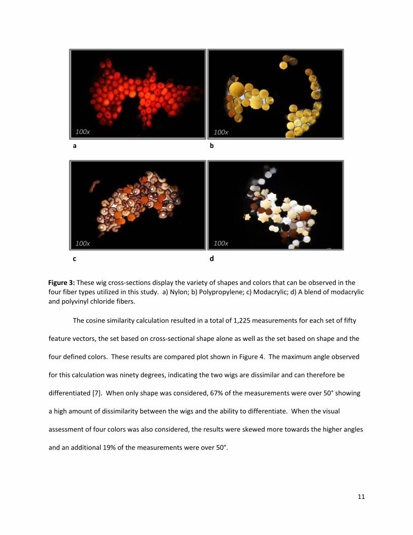
Through the use of the Joliff method, the cross-sectional shape analysis revealed shape to be

variable feature both between and within wigs. Figure 3 provides a representative example of the cross-

sections observed in each of the four possible fiber types: nylon, polypropylene, modacrylic, and a blend

of both modacrylic and polyvinyl chloride. As shown, wigs made of nylon exhibited irregular circles.

These cross-sections varied in size and shades of color. A small, dark core was also observed in a

number of the nylon fibers, potentially indicating a hollow core. Polypropylene wigs exhibited circular

cross-sections in various sizes. Only one of the four polypropylene wigs contained two distinct colors,

while the others consisted of a single color. Wigs made of either 100% modacrylic or a blend of

modacrylic and polyvinyl chloride fibers showed a range from one to as many as six different shapes

within a single wig, with a mode of two. The most popular cross-sectional shapes were horseshoe and

dog bone, followed by lobular.

10

c d

Figure 3: These wig cross-sections display the variety of shapes and colors that can be observed in the four fiber types utilized in this study. a) Nylon; b) Polypropylene; c) Modacrylic; d) A blend of modacrylic and polyvinyl chloride fibers.

The cosine similarity calculation resulted in a total of 1,225 measurements for each set of fifty

feature vectors, the set based on cross-sectional shape alone as well as the set based on shape and the

four defined colors. These results are compared plot shown in Figure 4. The maximum angle observed

for this calculation was ninety degrees, indicating the two wigs are dissimilar and can therefore be

differentiated [7]. When only shape was considered, 67% of the measurements were over 50° showing

a high amount of dissimilarity between the wigs and the ability to differentiate. When the visual

assessment of four colors was also considered, the results were skewed more towards the higher angles

and an additional 19% of the measurements were over 50°.

a b

100 x 100 x

100 x 100 x

11

Figure 4: The results of the cosine similarity calculations are compared for the two sets of feature vectors: cross-sectional shape alone, and shape and color combined. 3.2 Fourier Transform Infrared Spectroscopy (FTIR)

Four types of fibers were characterized by FTIR. A total of thirty-seven wigs out of fifty (74.0%)

were identified as modacrylic or a blend of modacrylic and polyvinyl chloride fibers. Nine wigs were

made of nylon and the last four of polypropylene.

Potential groupings for subsequent sub-classification were then determined by visual

assessment and statistical analyses of the infrared spectra. Utilization of the first derivatives of each

spectrum in the analyses, rather than raw data, displayed the rate of change in absorption across all

wavenumbers, ultimately providing better resolution of the spectral features.

Statistical analysis was first conducted on the 555 total spectra collected from both modacrylic

wigs and blended modacrylic and polyvinyl chloride wigs. By plotting the percent relative standard

deviation of the infrared absorbance at each wavenumber, it was found that the differences in the

spectra were driven by absorption peaks relative to the general polymeric class rather than subclasses.

This observation was confirmed when PCA was performed on this data. The strong absorption peak at

about 2240cm-1 found only in the modacrylic fibers accounted for the majority of the variance, followed

by peaks at 2850cm-1 and 1450cm-1 found only in the polypropylene fibers.

12

Hereafter, PCA was conducted on only the preprocessed, first derivatives of the 450 modacrylic

spectra to determine potential subclasses of modacrylics. When considering the entire spectrum from

4000-650cm-1, twenty-two principal components (PCs) described 90.3% of the total variance in the data

set. Thus, the 3,328 dimensions excluded from the original 3,350 only accounted for approximately 10%

of the data’s structure. Groupings were visible in a plot of the first two PCs, but clearer separation of

these groupings was achieved when the spectral data was further divided.

The dataset was first divided to consider only the fingerprint region from 1800-650cm-1.

Through PCA, the first eighteen PCs described 90.1% of the dataset’s total variance. The 18-dimensional

structure is obviously too high in dimensionality to plot, but it was informative to have a physical graph

of the data. Therefore, a plot of the first two PCs, accounting for 36.3% of the variance, is shown in

Figure 5 to give a better visual assessment of the subsequent groupings. Because only a small amount

of the total variance is shown, conclusions in regards to the number of groupings and the factors driving

their separation could not be drawn.

Figure 5: The first derivatives of the modacrylic spectra fingerprint region (1800-650cm-1), shown in a plot of the first two PCs (36.3% of the total variance). The numbers at each data point label the particular spectrum.

13

The modacrylic dataset was then divided to consider only the beginning alkane region from

4000-2600cm-1. With this final PCA, only ten PCs were needed to cover 90.5% of the total variance.

The first two PCs showing 60.9% is plotted in Figures 6. Once again, potential groupings can be

observed, but a higher amount of total variance should be observed in order to draw further

conclusions.

Figure 6: The first derivatives of the modacrylic spectra alkane region (4000-2600cm-1), shown in a plot of the first two PCs (60.9% of the total variance). The numbers at each data point label the particular spectrum.

After performing PCA, further analysis involving Ward’s Method of HCA was conducted to more

accurately define clusters and thereby define subsequent subclasses of modacrylic fibers. The

modacrylic dataset considering only the fingerprint region from 1800-650cm-1 was subject to HCA first.

The resulting cluster dendrogram is shown in Figure 7. The y-axis indicates the distance between

different groupings, whereas the connections show where successive splits take place between spectra.

Figure 8 was generated next as a plot of the linkage distances between each spectrum. The initial gap,

or jump, in successive linkage distances observed at a distance of ten indicates the height at which to cut

the tree to form clusters. Once the dendrogram was cut at a height of ten, three clusters were

indicated. These clusters are outlined in red in Figure 7.

14

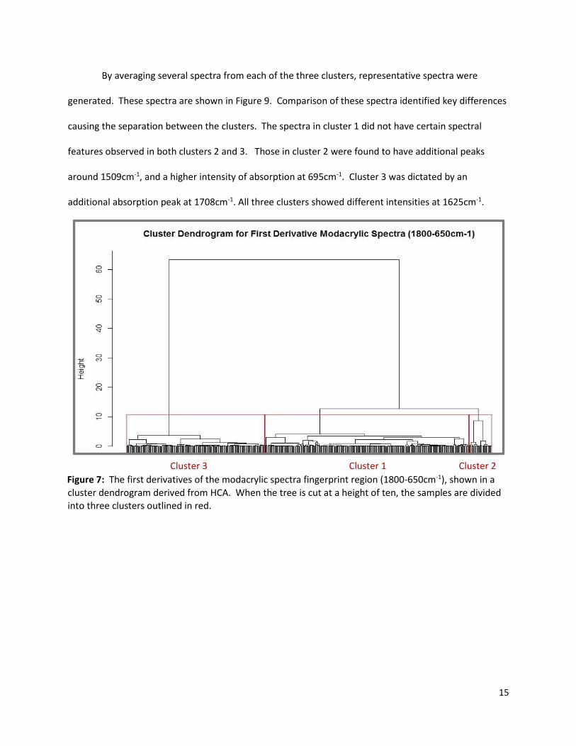
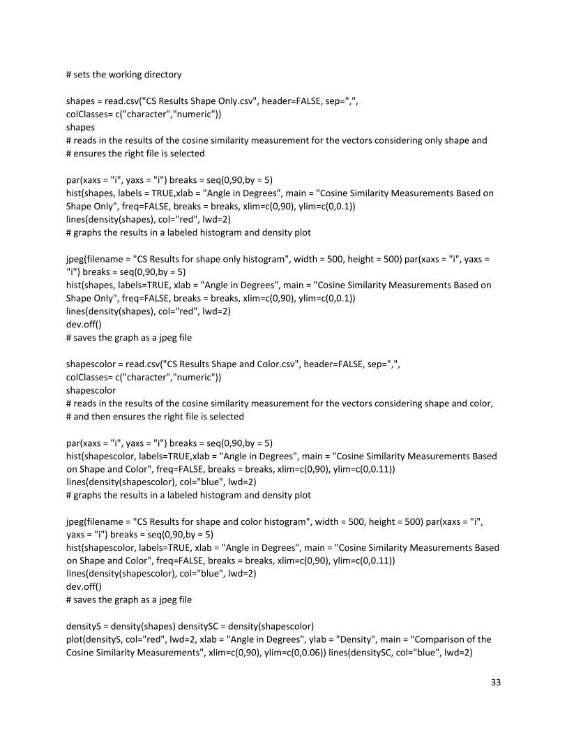
By averaging several spectra from each of the three clusters, representative spectra were

generated. These spectra are shown in Figure 9. Comparison of these spectra identified key differences

causing the separation between the clusters. The spectra in cluster 1 did not have certain spectral

features observed in both clusters 2 and 3. Those in cluster 2 were found to have additional peaks

around 1509cm-1, and a higher intensity of absorption at 695cm-1. Cluster 3 was dictated by an

additional absorption peak at 1708cm-1. All three clusters showed different intensities at 1625cm-1.

Cluster 3 Cluster 1 Cluster 2 Figure 7: The first derivatives of the modacrylic spectra fingerprint region (1800-650cm-1), shown in a cluster dendrogram derived from HCA. When the tree is cut at a height of ten, the samples are divided into three clusters outlined in red.

15

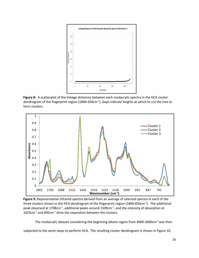
Figure 8: A scatterplot of the linkage distances between each modacrylic spectra in the HCA cluster dendrogram of the fingerprint region (1800-650cm-1). Gaps indicate heights at which to cut the tree to form clusters.

Figure 9: Representative infrared spectra derived from an average of selected spectra in each of the three clusters shown in the HCA dendrogram of the fingerprint region (1800-650cm-1). The additional peak observed at 1708cm-1, additional peaks around 1509cm-1, and the intensity of absorption at 1625cm-1 and 695cm-1 drive the separation between the clusters.

The modacrylic dataset considering the beginning alkane region from 4000-2600cm-1 was then

subjected to the same steps to perform HCA. The resulting cluster dendrogram is shown in Figure 10.

0

0.1

0.2

0.3

0.4

0.5

0.6

0.7

0.8

0.9

1

1801 1705 1608 1512 1416 1319 1223 1126 1030 933 837 741

Abso

rban

ce

Wavenumber (cm-1)

Cluster 1Cluster 2Cluster 3

16

The scatterplot of the linkage distances between spectra, Figure 11, showed a jump around a distance of

one. Therefore, the dendrogram was cut a height of one which revealed three clusters. These clusters

are outlined in red in Figure 10.

Representative spectra, shown in Figure 12, were generated in the same fashion and gave a

visual depiction of the differences between clusters. The three clusters were primarily separated by the

amount of absorption from 3700-3300cm-1, particularly by the intensity difference between the peaks at

3630cm-1 and 3530cm-1. Cluster 2 also seems to have a stronger peak at 3630cm-1 rather than a broader

curve.

Cluster 3 Cluster 1 Cluster 2 Figure 10: The first derivatives of the alkane region of the modacrylic spectra alkane region (40002600cm-1), shown in a cluster dendrogram derived from HCA. When the tree is cut at a height of one, the samples are divided into three clusters outlined in red.

17

Figure 11: A scatterplot of the linkage distances between each modacrylic spectra in the HCA cluster dendrogram of the alkane region (4000-2600cm-1). Gaps indicate heights at which to cut the tree to form clusters.

Figure 12: Representative infrared spectra derived from an average of selected spectra in each of the three clusters shown in the HCA dendrogram of the alkane region (4000-2600cm-1). The clusters were primarily separated by the amount of absorption from 3700-3300cm-1, particularly by the intensity difference between the peaks at 3630cm-1 and 3530cm-1.

0

0.1

0.2

0.3

0.4

0.5

0.6

0.7

0.8

0.9

1

3998 3901 3805 3708 3612 3516 3419 3323 3226 3130 3033 2937 2841 2744 2648

Abso

rban

ce

Wavenumber (cm-1)

Cluster 1Cluster 2Cluster 3

18

3.3 Thin-Layer Chromatography (TLC)

Observations confirmed that the fiber class dictated the type of chemical used to provide color.

All modacrylic and polyvinyl chloride fibers were found to contain basic dye types, while nylon fibers

contained acidic types as suggested by the literature [13]. The wigs made of polypropylene fibers were

pigmented as no color could be extracted.

The wigs made of modacrylic, as well as those having the modacrylic and polyvinyl chloride

blend, exhibited a number of colors on the corresponding TLC plates. The basic dyes contained two to

twelve spots. Both the brown and blonde wigs of these fiber types had a mode of three spots, while

wigs that appeared black surprisingly had a mode of six. The majority of the spots were shades of red,

yellow and blue. As expected, blonde wigs were observed to have more yellow than any other color. A

portion of the black and brown wigs also exhibited orange bands. Twenty-eight of the thirty-seven wigs

of these fiber types (75.7%) had a blue fluorescent band near the edge of the solvent front. Pink and

yellow fluorescent bands were less commonly observed, oftentimes in addition to the blue. An

example of the TLC results for a brown modacrylic wig is shown in Figure 13.

19

b Figure 13: The two replications that were done for each of the three samples cut from the same brown modacrylic wig. The control and blank are to the left of the plate. a) The plate viewed under white light. b) The same TLC plate viewed with ultraviolet light at 365nm showing additional blue and yellow fluorescent spots.

In relation to the nylon wigs, the acidic dyes contained as many as six spots with a mode of four,

regardless of the wig’s appeared color. Similarly to the modacrylic wigs, the majority of the contents

were shades of red, yellow and blue. The blonde nylon wigs were observed to have more red spots

rather than yellow in comparison to the modacrylics. Orange spots were often observed in the brown

wigs in addition to black ones. With regards to the blue fluorescent band often found in the modacrylic

wigs, only four of the nine nylon wigs had this spot. Pink, yellow, and green fluorescent bands were

` a

20

each observed once in separate wigs. An example of the TLC results for a brown nylon wig is shown in

Figure 14.

b Figure 14: The two replications that were done for each of the three samples cut from the same brown nylon wig. The control and blank are to the left of the plate. a) The plate viewed under white light showing red and yellow spots. b) The same TLC plate viewed with ultraviolet light at 365nm showing additional blue and green fluorescent spots. 4. Discussion

4.1 Polarized Light Microscopy and Cross-Sectional Shape Analysis

Results showed the modacrylic fiber had the most variation and highest density of delustrants

and fisheyes, factors which could be used for comparative purposes. These physical features, however,

cannot be used for fiber type identification [5]. With regards to optical properties, the literature

suggests both acrylic and modacrylic fibers had predominantly negative signs of elongation when

a

21

observed under double polarization conditions [5]. However, most modacrylics today are optically

positive as was observed in this study. This is due to a lower amount of polyacrylonitrile used in

production [5]. A modacrylic fiber is required to contain 35%-85% polyacrylonitrile to distinguish it from

acrylic fibers according to the United States Federal Trade Commission standards. The amount of

polyacrylonitrile is said to dictate the fiber’s sign of elongation and, although not observed in this study,

could be an additional source of variation among modacrylics [5].

Through the author’s previous research, there was found to be overlap in measurements of the

fibers’ width and cross-sectional surface area. Due to the overall high degree of intra-variability, and a

low degree of inter-variability, it was determined that both of these measurements were not useful in

the discrimination between wigs.

Cross-sectional shape, however, has been observed in the past and current study to be a

variable feature both within and between wigs which aids in the wig’s characterization. The fiber’s

shape is a result of one of three factors: engineering for a specific end use, an attribute in the

manufacturing process, or accidental causes such as crushing [3]. Certain cross-sectional shapes that are

difficult to make, and thus expensive, have been patented by various manufacturers [3]. These

research results have indicated that the shape is foremost dictated by the fiber type. Polypropylene

fibers are uniformly circular, while nylon fibers are irregular in shape. The highest degree of variability is

found in the modacrylic and blended wigs as combinations of eleven different shapes were observed. A

single wig was found to contain as many as six of these different shapes.

By using the presence of cross-sectional shapes to populate feature vectors and subsequently

measuring the angle of similarity between them, an objective method of differentiation was achieved.

However, it must be noted that the discriminating power of the described method may be weighted

heavily on sample size. The combination of shapes and colors within the wig greatly influences the

cosine similarity measurement. Therefore, a larger sample size is necessary to properly observe the

22

overall combination. At the same time, only four colors were used in this study to describe the cross

sections. Additional colors would increase the ability to differentiate between samples, which may

allow for a smaller sample size. A blind study could be conducted to further examine the overall

discrimination power of this proposed method.

Future research into this area of cross-sectional shape analysis may allow for the production of a

contextual search engine or searchable database similar to 'SoleMate', Foster + Freeman's footwear

database [15]. The database would help to identify a wig from synthetic fibers recovered from a crime

scene. Each record in the database would contain all relevant manufacturer information, several images

of the wig itself and its cross-section, and most importantly a set of feature codes that allow for search

operations [15]. To use the database, the scientist would identify the presence of shapes and colors in

the cross-section of the questioned sample. This process will develop a feature code similar to the

feature vectors used in this study. Upon submission, the system will then search the database for wigs

having similar feature codes and present the results that best match in descending order for the

scientist to examine [15]. The database would have to be updated periodically as new wigs are

introduced to the market.

4.2 Fourier Transform Infrared Spectroscopy (FTIR)

FTIR was used to determine the general polymeric class and subclass when possible [10]. The

infrared data confirmed modacrylic to be the most popular fiber type in wigs. It was unexpected,

though, to find so many wigs made of a blend of both modacrylic and polyvinyl chloride fibers. There

were, in fact, eight instances where the label indicated the material was 100% modacrylic or kanekalon,

but found to also contain polyvinyl chloride. Kanekalon is a trademark for a Japanese-manufactured

modacrylic fiber which is used extensively in making wigs and hairpieces. Kanekalon representatives

have indicated this blend is often created for aesthetic style and color purposes [4].

23

Because modacrylic fibers were the most common, this fiber type became the focus of further

assessment and statistical analyses. The infrared spectrum of a modacrylic fiber can be influenced by

the amount of acrylonitrile, the type of co-monomer, termonomers added to provide dye sites, the

presence of solvent residues, dyes, and additives like flame retardant materials [3].

The amount of acrylonitrile in the fiber is shown by a large absorption peak at about 2240cm-1.

This peak is indicative of acrylic and modacrylic fibers as it is influenced by the number of nitrile (C=N)

units [3]. Likewise, the smaller peak at 695cm-1 is indicative of C-Cl bonding [3]. This peak along with

the CH absorption stretch from 1254-1243cm-1 and the overall configuration from 1360-1214cm-1 reveal

the type of co-monomer is vinyl chloride (CH2=CHCl) [3]. All modacrylic fibers in this study contained

this same co-monomer, however, the differences observed in the intensity of absorption at 695cm-1 may

be due to resins containing different amounts of the vinyl chloride [3]. The presence of vinyl acetate is

illustrated by a peak at 1733cm-1 [3]. This ester is added to the fiber as a plasticizer, an additive that

increases the fiber’s plasticity or fluidity [3]. An aliphatic sulphonate, shown at 1038cm-1, is used as a

termonomer to produce dye sites [3]. Because this peak is coupled with another at 1003cm-1, the

termonomer in this study is specifically sodium styrene sulphonate [3]. These spectral features were

relatively similar across all of the modacrylic wig fibers.

Principal component analysis coupled with hierarchical clustering analysis, however, was able to

indicate subsequent groupings and possible areas within the spectra that can be used for more selective

characterization. When conducting statistical analyses on the fingerprint region (1800-650cm-1), the

modacrylics were primarily separated by the presence of a peak at 1708cm-1. This peak may be

attributed to residue from the acetone solvent used in the manufacturing process [3]. The samples

were also separated by the intensity of absorption at 1625cm-1 and 695cm-1, which is indicative of the

amount of water and the amount of CCl bonding within the fiber respectively [3]. The HCA dendrogram

24

clustered spectra from three wigs having small peaks at and around 1509cm-1. These are to be

considered dye peaks [16].

When PCA and HCA were carried out on the alkane region (4000-2600cm-1), the fibers were

separated by differences in the amount of absorption from 3700-3300cm-1. This stretch can be

attributed to the number of O-H bonds within the fiber [17]. Unfortunately, no other references to this

stretch can be found in previous literature in order to identify the source of the varying O-H bonds. It

must also be noted that the length of the y-axis in the HCA dendrogram for the alkane region was

considerably smaller than that of the fingerprint region. This fact indicates the differences observed

from 3700-3300cm-1 are much smaller in comparison to those observed from 1800-650cm-1 [12].

4.3 Thin-Layer Chromatography (TLC)

According to previous literature, a solution of formic acid, water 1:1 should be used to extract

basic dye from modacrylic fibers [13]. This extraction solution, however, was unsuccessful when applied

to these types of wigs as shown in Figure 15a. Only when formic acid alone was applied, did the dye

separate from the fiber. The higher concentration of formic acid was successful in extraction, but the

spots did not separate on the TLC plate as seen in Figure 15b. Multiple eluent solutions were applied at

this point in an attempt to achieve better separation, but they were found to be ineffective [13]. A

solution of pyridine, water 4:3 was then utilized, as illustrated in Figure 15c, as it is also a suggested

extraction solution [13]. This solution extracted the dye successfully, and gave better separation of the

spots. The best results were achieved, however, when a solution of pyridine, water 2:1 was introduced,

shown in Figure 15d. Subsequently, this solution was applied to each wig as well as straight formic acid

to continuously observe the differences in the results. A representative example of the TLC plates

developed for each sample is shown in Figure 16.

25

c d

Figure 15: The TLC results from a brown modacrylic wig when different extract solutions were used. a) A solution of formic acid,water 1:1; b) Formic acid; c) A solution of pyridine, water 4:3; d) A solution of pyridine, water 2:1.

Figure 16: A representative example of the TLC results achieved for each wig using both a) pyridine,water 2:1 and b) formic acid as an extraction solution. These particular results are from a brown modacrylic wig.

a b

a b

26

Pyridine, water 2:1 extraction solution is commonly used in the examination of pen and printer

inks [18]. Further research may find that the dyes applied to wig fibers have more in common with

writing inks, than with the dyes used on garments and household items. A difference in the dye

application process may also be possible.

Most textile fibers do contain multiple components to obtain the desired shade, but such

complex dye patterns were not expected in brown, blonde, and especially black wigs [19]. The dye was

observed to contain as many as twelve different spots of color, including those with fluorescent

properties. This high degree of intra-variability may again be contributed to the composition of the wig.

In addition to TLC, microspectrophotometry (MSP) is a widely accepted method for color

comparisons. Some scientists prefer MSP as it is a nondestructive method resulting in quantitative

results [19]. MSP has also been reported to distinguish fibers that were not previously differentiated by

TLC [19]. MSP, however, provides limited information where fibers are either extremely light or

extremely dark as in the case of blonde, dark brown and black wigs [19]. A study involving MSP analysis

of synthetic wig fibers was recently conducted and showed that twenty-six of the sixty-two fibers

sampled (42%) were left indistinguishable after MSP was performed [4]. Almost half of this

undetermined group was composed of brown and black fibers.

In comparison, seven of the thirty-seven modacrylic wigs (19%) could not be differentiated after

TLC in this study based on the location and color of the spots. These wigs came from a sampling of

brown, modacrylic wigs retailed by the same manufacturer. All nine of the nylon wigs, on the other

hand, could be differentiated. It may be possible to further differentiate between wigs dyes by

performing MSP on the individual bands on the TLC plates. Results may show differences in the various

shades of a single color.

27

4.4 Suggested Protocol for Sampling and Analysis

Observations indicated the wigs had a high degree of intra-variability. This intra-variability is due

to the nature of the wig’s composition. As mentioned, various types and colors of fibers may be

blended throughout one wig so that it may appear more natural looking for cosmetic use [2]. This fact

highlights the need to analyze multiple known fibers from the same wig, as a single fiber is not a

representative sample. A maximum of two different fiber types, four visually determined colors, and six

different cross-sectional shapes were observed within a single wig. Accordingly, a sample size of at least

ten known fibers should be taken. More fibers will be desirable particularly when attempting to

perform TLC analysis on blonde wigs as the resulting extract is rather light in color. When sampling from

a wig, fibers should be cut from various locations in order to properly observe its degree of variability.

Further research into the frequency and persistence of wig fibers would indicate the plausible sample

size at a crime scene and may help to estimate when the fibers were deposited.

As aforementioned, TLC results could not differentiate between seven brown modacrylic wigs

having the same manufacturer. However, HCA performed on the FTIR spectra was able to exclude one of

these wigs leaving instead a group of six. Upon the application of cross-sectional shape analysis, only

five of these wigs were left indifferentiable. This analysis was also able to further divide these five wigs

into a group of two and a group of three that could not be differentiated. Given these results, it can be

concluded that cross-sectional shape and color are a wig’s most variable features; therefore cross-

sectional shape analysis is the most discriminatory analytical method for synthetic wigs. Therefore,

once comparison microscopy techniques have been exhausted and if the sample size allows, cross-

sectional shape analysis should be conducted first. Fortunately, performing this method requires a

minimal amount of time and resources. If a conclusion cannot be drawn after this analysis or if

supporting evidence is desired, then FTIR should be applied followed by TLC.

28

5. Conclusion

This study identified microscopical and chemical features of synthetic wigs that trace evidence

examiners can use for characterization and comparison, by means of their currently available

instrumentation. The analysis of cross-sectional shape proved to be useful in the differentiation

between wigs due to the high amount of both inter- and intra-variability. This capability increased when

cross-sectional shape was coupled with a visual assessment of color. Infrared spectroscopy confirmed

modacrylic to be the most prominent fiber type in synthetic wigs. Principal component analysis in

agreement with hierarchical clustering analysis indicated subgroupings of modacrylics and specific areas

within their FTIR spectra where discriminating characteristics could be observed such as the presence of

solvent residue, dyes and the overall amount of other additives. With regards to the dye content of the

fiber, it was concluded that a solution of pyridine, water 2:1 served as the best extraction solution for

both modacrylic and nylon wig fibers. Final TLC results indicated there is a wider range of complex dyes

that are applied than previously expected. Due to the particular source of high variability, only seven of

the fifty wigs (14%) could not be differentiated after TLC was performed. Out of this group of seven,

only a group of two and a group of three wigs (10%)were left indifferentiable upon the application of

cross-sectional shape analysis. It is therefore concluded that these features are the most discriminatory

for synthetic wigs, and this analysis should be conducted first. The additional research suggested may

help to further individualize these wigs.

29

6. References

[1] Cheesbrough, M. J. "Wigs." British Medical Journal 299 (1989): 1455-456. Print.

[2] Ballou, Susan. "Wigs and the Significance of One Fiber." Mute Witnesses: Trace Evidence Analysis. By Max M. Houck. San Diego, CA: Academic, 2001. 21-46. Print.

[3] Grieve, M.c., and R.m.e. Griffin. "Is It a Modacrylic Fibre?" Science & Justice 39.3 (1999): 151-62. Print.

[4] Long, Holly, Sarah Walbridge-Jones, and Kacie Lundgren. “Synthetic Wig Fibers: Analysis & Differentiation from Human Hairs.” Journal of American Society of Trace Evidence Examiners 5.1. (2014): 2-21. Print.

[5] Palenik, Samuel J. "Chapter 7: Microscopical Examination of Fibres." Forensic Examination of Fibres. By James R. Robertson and Michael C. Grieve. 2nd ed. London: Taylor & Francis, 1999. 153-77. Print.

[6] Scientific Working Group on Materials Analysis Trace Evidence. Forensic Fiber Examinations Guidelines. 1999. Print.

[7] Varmuza, Kurt, and Peter Filzmoser. Introduction to Multivariate Statistical Analysis in Chemometrics. Boca Raton: CRC, 2009. Print.

[8] Murrell, Paul. R Graphics. Boca Raton: Chapman & Hall/CRC, 2006. Print.

[9] Tungol, Mary W., Edward G. Bartick, and Akbar Montaser. "The Development of a Spectral Database for the Identification of Fibers by Infrared Microscopy." Applied Spectroscopy 44.4 (1990): 543-49. Print.

[10] Kirkbride, Kenneth P., and Mary W. Tungol. "Chapter 8: Infrared Microspectroscopy of Fibres." Forensic Examination of Fibres. By Michael C. Grieve and James R. Robertson. 2nd ed. London: Taylor & Francis, 1999. 179-222. Print.

[11] Wehrens, Ron. Chemometrics with R: Multivariate Data Analysis in the Natural Sciences and Life Sciences. Heidelberg: Springer, 2011. Print.

[12] Murtagh, Fionn, and Pierre Legendre. "Ward's Hierarchical Clustering Method: Clustering Criterion and Agglomerative Algorithm." 2 (2011): 1-20. Cornell University Library. Web.

[13] Wiggins, Kenneth G. "Chapter 11: Thin-Layer Chromatographic Analysis for Fibre Dyes." Forensic Examination of Fibres. By Michael C. Grieve and James R. Robertson. 2nd ed. London: Taylor & Francis, 1999. 291-310. Print.

[14] Beattie, I.b., H.l. Roberts, and R.j. Dudley. "Thin-layer Chromatography of Dyes Extracted from Polyester, Nylon and Polyacrylonitrile Fibres." Forensic Science International 17.1 (1981): 57-69. Print.

30

[15] "50th SoleMate Footwear Database Released." Foster + Freeman. N.p., 11 July 2013. Web.

[16] Grieve, Michael C., R.m.e. Griffin, and R. Malone. “Characteristic Dye Absorption Peaks Found in the FTIR Spectra of Coloured Acrylic Fibers.” Science & Justice 38 (1998): 27-37. Print.

[17] Coates, John, and Robert A. Meyers. "Interpretation of Infrared Spectra, A Practical Approach." Encyclopedia of Analytical Chemistry: Applications, Theory, and Instrumentation. Chichester: Wiley, 2000. 10815-0837. Print.

[18] Tsutsumi, Kazuhiro, and Kazuya Ohga. "Analysis of Writing Ink Dyestuffs by TLC and FT-IR and Its Application to Forensic Science." Analytical Sciences 14.2 (1998): 269-74. Print.

[19] Goodpaster, John V., and Elisa A. Liszewski. "Forensic Analysis of Dyed Textile Fibers." Analytical and Bioanalytical Chemistry 394.8 (2009): 2009-018. Print.

31

Appendix A – R scripts

1. R-Script for computing the cosine similarity measurement between feature vectors developed from the cross-sections. File names were changed when the different sets of feature vectors were analyzed.

library(aspace) # this package is necessary to compute the cosine of the angle in degrees setwd("C:/Users/Theresa/Documents/Thesis/Wig Cross Sections") getwd() # sets the working directory shapes = read.csv("cross section feature vectors_shape only.csv", header=FALSE, sep=",", colClasses=c("character","numeric")) shapes # reads in the data for the cross sections vectors and ensures the right file is selected attach(shapes) # allows creation of subsets from the shapes file wig1 = shapes[2:12,2] wig1 wig2 = shapes[14:24,2] wig2 # specifies the data for each wig by indicating the row and column numbers and ensures we have the # right vectors mag1 = sqrt(t(wig1)%*%wig1) mag2 = sqrt(t(wig2)%*%wig2) # computes the magnitude for the wig vectors, by computing the square root of the transposed vector # multiplied by the original num1t2 = t(wig1)%*%wig2 # multiplies the transposed wig 1 vector by wig 2 vector and serves as the numerator for the cosine # similarity equation wig1wig2 = num1t2/(mag1%*%mag2) # divides the calculated numerator by the multiplied magnitudes of the vectors acos_d(wig1wig2) # computes the inverse cosine of the angle in degrees giving the end measurement of similarity 2. R-script for displaying the results of the cosine similarity measurements between cross-section

feature vectors in both histograms and density plot setwd("C:/Users/Theresa/Documents/Thesis/Stat Analysis") getwd()

32

# sets the working directory shapes = read.csv("CS Results Shape Only.csv", header=FALSE, sep=",", colClasses= c("character","numeric")) shapes # reads in the results of the cosine similarity measurement for the vectors considering only shape and # ensures the right file is selected par(xaxs = "i", yaxs = "i") breaks = seq(0,90,by = 5) hist(shapes, labels = TRUE,xlab = "Angle in Degrees", main = "Cosine Similarity Measurements Based on Shape Only", freq=FALSE, breaks = breaks, xlim=c(0,90), ylim=c(0,0.1)) lines(density(shapes), col="red", lwd=2) # graphs the results in a labeled histogram and density plot jpeg(filename = "CS Results for shape only histogram", width = 500, height = 500) par(xaxs = "i", yaxs = "i") breaks = seq(0,90,by = 5) hist(shapes, labels=TRUE, xlab = "Angle in Degrees", main = "Cosine Similarity Measurements Based on Shape Only", freq=FALSE, breaks = breaks, xlim=c(0,90), ylim=c(0,0.1)) lines(density(shapes), col="red", lwd=2) dev.off() # saves the graph as a jpeg file shapescolor = read.csv("CS Results Shape and Color.csv", header=FALSE, sep=",", colClasses= c("character","numeric")) shapescolor # reads in the results of the cosine similarity measurement for the vectors considering shape and color, # and then ensures the right file is selected par(xaxs = "i", yaxs = "i") breaks = seq(0,90,by = 5) hist(shapescolor, labels=TRUE,xlab = "Angle in Degrees", main = "Cosine Similarity Measurements Based on Shape and Color", freq=FALSE, breaks = breaks, xlim=c(0,90), ylim=c(0,0.11)) lines(density(shapescolor), col="blue", lwd=2) # graphs the results in a labeled histogram and density plot jpeg(filename = "CS Results for shape and color histogram", width = 500, height = 500) par(xaxs = "i", yaxs = "i") breaks = seq(0,90,by = 5) hist(shapescolor, labels=TRUE, xlab = "Angle in Degrees", main = "Cosine Similarity Measurements Based on Shape and Color", freq=FALSE, breaks = breaks, xlim=c(0,90), ylim=c(0,0.11)) lines(density(shapescolor), col="blue", lwd=2) dev.off() # saves the graph as a jpeg file densityS = density(shapes) densitySC = density(shapescolor) plot(densityS, col="red", lwd=2, xlab = "Angle in Degrees", ylab = "Density", main = "Comparison of the Cosine Similarity Measurements", xlim=c(0,90), ylim=c(0,0.06)) lines(densitySC, col="blue", lwd=2)

33

legend(10, 0.04, c("Shape Only", "Shape and Color"), col=c("red", "blue"), lwd=1, cex=1) # graphs the two density plots together in one for comparison purposes jpeg(filename = "CS Results comparison of density", width=500, height=500) plot(densityS, col="red", lwd=2, xlab = "Angle in Degrees", ylab = "Density", main = "Comparison of the Cosine Similarity Measurements", xlim=c(0,90), ylim=c(0,0.06)) lines(densitySC, col="blue", lwd=2) legend(10, 0.04, c("Shape Only", "Shape and Color"), col=c("red", "blue"), lwd=1, cex=1) # saves the graph as a jpeg file 3. R-script for performing PCA on the chosen FTIR data. File names were changed as analysis was

conducted on different regions of the data. setwd("C:/Users/Theresa/Documents/Thesis/FTIR") getwd() # sets the working directory library(scatterplot3d) # loads package needed for 3d plots raw.FTIR = read.csv("data_no2_MA fingerprint_first.csv", header=TRUE, sep=",", row.names=1) head(raw.FTIR) # reads in the file and confirms only the first 6 rows of each column rather than consuming the # workspace with the whole file sc.FTIR = apply(raw.FTIR,2,function(x) (x-mean(x))/sd(x)) # mean centers the data and divides it by the standard deviation to get unit variance (This step is # needed for the correlation matrix.) cor.FTIR = cor(sc.FTIR) head(cor.FTIR) # computes the correlation matrix eigen.FTIR = eigen(cor.FTIR) head(eigen.FTIR) # computes eigenvalues and eigenvectors FTIR.var = (eigen.FTIR$values/(nrow(raw.FTIR)-1)) FTIR.totalvar = sum(FTIR.var) FTIR.relvar = FTIR.var/FTIR.totalvar PC.var = 100*round(FTIR.relvar, digits = 3) PC.var[1:5] sum(PC.var[1:5]) # computes total and percent variance for data and each PC. Shows amount of variance in first 5 PCs. pc1.var = 100*(eigen.FTIR$values[1]/sum(eigen.FTIR$values)) pc1.var pc2.var = 100*(eigen.FTIR$values[2]/sum(eigen.FTIR$values)) pc2.var pc3.var = 100*(eigen.FTIR$values[3]/sum(eigen.FTIR$values)) pc3.var pc4.var = 100*(eigen.FTIR$values[4]/sum(eigen.FTIR$values)) pc4.var

34

pc5.var = 100*(eigen.FTIR$values[5]/sum(eigen.FTIR$values)) pc5.var pc1.var+pc2.var+pc3.var+pc4.var+pc5.var # double checks the variance codes: eigenvalue for the PC divided by total variance equals percent # variance in that PC par(mfrow= c(2,2)) barplot(FTIR.relvar[1:10], main = "PC Variances", names.arg = paste("PC", 1:10)) # creates a bar graph for amount of variance in first 10 PCs jpeg(filename = "PC Variances_no2_MA fingerprint_first.jpg", width = 256, height = 356) barplot(FTIR.relvar[1:10], main = "PC Variances", names.arg = paste("PC", 1:10)) dev.off() # saves PC variances bar graph as jpeg file loadings = eigen.FTIR$vectors scores = sc.FTIR %*% eigen.FTIR$vectors # computes the loadings and scores for PCA plot(scores[,1:2], type = "n", main = "PC1 v PC2", xlab = paste("PC 1(", PC.var[1], "%)", sep = ""), ylab = paste("PC 2(", PC.var[2], "%)", sep = "")) # points(scores[,1:2]) # creates a biplot for PC1 vs PC2 showing scores. The points function can be used instead of labeling the # spectra with text samples = read.csv("sample names_no2_MA spectrum_first.csv", header=TRUE, sep=",", colClasses=c("character")) text(scores[,1],scores[,2], rownames(samples), col="blue", cex=0.7) # plots the scores as samples using text. Each number represents a different spectrum scatterplot3d(scores[,1:3], main = "PCA plot for First Derivative Modacrylic Spectra (1800-650cm-1)", xlab = paste("PC 1(", PC.var[1], "%)", sep = ""), ylab = paste("PC 2(", PC.var[2], "%)", sep = ""), zlab = paste("PC 3(", PC.var[3], "%)", sep = ""),pch=16, highlight.3d=TRUE, type="h") # creates a 3d plot for PC1 vs PC2 vs PC3 samples = read.csv("sample names_no2_MA spectrum_first.csv", header=TRUE, sep=",", colClasses=c("character")) text(scores[,1],scores[,2],scores[,3], rownames(samples)) # plots the scores as samples using text for 3d plot jpeg(filename = "PC1vPC2_no2_MA fingerprint_first.jpg", width = 500, height = 500) plot(scores[,1:2], type = "n", main = "PC1 v PC2 for First Derivative Modacrylic Spectra (1800-650cm-1)", xlab = paste("PC 1(", PC.var[1], "%)", sep = ""), ylab = paste("PC 2(", PC.var[2], "%)", sep = "")) samples = read.csv("sample names_no2_MA spectrum_first.csv", header=TRUE, sep=",", colClasses=c("character")) text(scores[,1],scores[,2], rownames(samples), col="blue", cex=0.7)

35

dev.off() # saves biplot for PC1 v PC2 as jpeg file jpeg(filename = "3d PCA plot_no2_MA fingerprint_first.jpg", width = 500, height = 500) scatterplot3d(scores[,1:3], main = "PCA plot for First Derivative Modacrylic Spectra (1800-650cm-1)", xlab = paste("PC 1(", PC.var[1], "%)", sep = ""), ylab = paste("PC 2(", PC.var[2], "%)", sep = ""), zlab = paste("PC 3(", PC.var[3], "%)", sep = ""),pch=16, highlight.3d=TRUE, type="h") samples = read.csv("sample names_no2_MA spectrum_first.csv", header=TRUE, sep=",", colClasses=c("character")) text(scores[,1],scores[,2],scores[,3], rownames(samples)) dev.off() # saves 3d PCA plot as jpeg file 4. R-script for performing HCA on both the fingerprint region and alkane region of the FTIR data setwd("C:/Users/Theresa/Documents/Thesis/FTIR") getwd() # sets the working directory ##HCA on the fingerprint region FTIR = read.csv("data_no2_MA fingerprint_first.csv", header=TRUE, sep=",", row.names=1) head(FTIR) # reads in the file and confirms only the first 6 rows of each column rather than consuming the # workspace with the whole file dist.FTIR = dist(FTIR, method = "euclidean") # computes the distance matrix using Euclidean distance distsq.FTIR = dist.FTIR^2 # squares the distance matrix as needed for Ward's method hca.FTIR = hclust(distsq.FTIR, method = "ward") # performs HCA on distance matrix using Ward's method plot(hca.FTIR, labels = row.names(FTIR), main = "Cluster Dendrogram for First Derivative Modacrylic Spectra (1800-650cm-1)", lwd = 0.5, cex = 0.5) rect.hclust(hca.FTIR, h=10, border="red") # plots the HCA dendrogram with red borders around the clusters plot(1:448, hca.FTIR$height, xlab = "Wig Samples", ylab = "Linkage Distance", main = "Linkage Distances for First Derivative Modacrylic Spectra (1800-650cm-1) ", type = "p") # plots linkage distances to determine at what distance to cut the tree hca.table.FTIR = cutree(hca.FTIR, h=10) table(hca.table.FTIR, row.names(FTIR))

36

# gives table showing which cluster each samples belongs to. The number of clusters depends on the # the height tree is cut at. ##HCA on the alkane region FTIR = read.csv("data_no2_MA beginning_first.csv", header=TRUE, sep=",", row.names=1) head(FTIR) dist.FTIR = dist(FTIR, method = "euclidean") distsq.FTIR = dist.FTIR^2 hca.FTIR = hclust(distsq.FTIR, method = "ward") plot(hca.FTIR, labels = row.names(FTIR), main = "Cluster Dendrogram for First Derivative Modacrylic Spectra (4000-2600cm-1)", lwd = 0.5, cex = 0.5) rect.hclust(hca.FTIR, h=1, border="red") plot(1:448, hca.FTIR$height, xlab = "Wig Samples", ylab = "Linkage Distance", main = "Linkage Distances for First Derivative Modacrylic Spectra (4000-2600cm-1)", type = "p") hca.table.FTIR = cutree(hca.FTIR, h=1) table(hca.table.FTIR, row.names(FTIR))

37

Appendix B – Representative photomicrographs of fibers

Figures 1 and 2: Photomicrographs of a nylon fiber from wig 044 under bright field and double polarization conditions.

Figures 3 and 4: Photomicrographs of a nylon fiber from wig 042 under bright field and double polarization conditions.

Figures 5 and 6: Photomicrographs of a polypropylene fiber from wig 051 under bright field and double polarization conditions.

38

Figures 7 and 8: Photomicrographs of a polypropylene fiber from wig 003 under bright field and double polarization conditions.

Figures 9 and 10: Photomicrographs of a modacrylic fiber from wig 009 under bright field and double polarization conditions.

Figures 11 and 12: Photomicrographs of a modacrylic fiber from wig 031 under bright field and double polarization conditions.

39

Figures 13 and 14: Photomicrographs of a polyvinyl chloride fiber from wig 016 under bright field and double polarization conditions.

Figures 15 and 16: Photomicrographs of a polyvinyl chloride fiber from wig 025 under bright field and double polarization conditions.

40

Appendix C – Representative photomicrographs of cross-sections

Figures 1 and 2: Cross-sections of nylon wigs 043 and 036, respectively

Figures 3 and 4: Cross-sections of polypropylene wigs 051 and 052, respectively

Figures 5 and 6: Cross-sections of modacrylic wigs 017 and 033, respectively

41

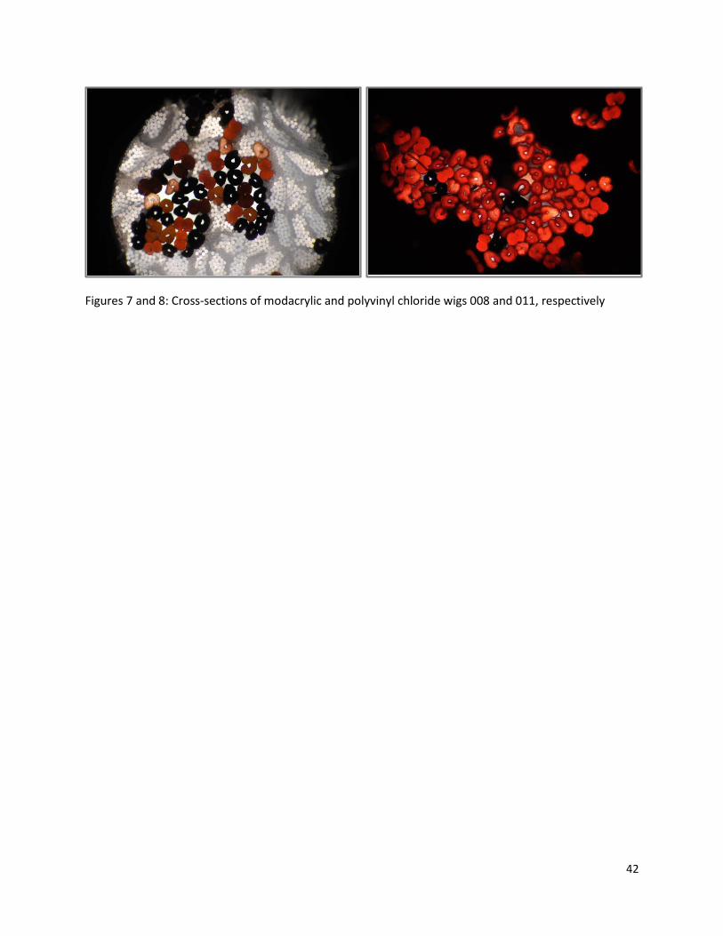
Figures 7 and 8: Cross-sections of modacrylic and polyvinyl chloride wigs 008 and 011, respectively

42

Appendix D – Representative FTIR spectra

Figure 1: FTIR spectra from nylon wigs 036 (top) and 039 (bottom)

Figure 2: FTIR spectra from polypropylene wigs 051 (top) and 005 (bottom)

43

Figure 3: FTIR spectra from modacrylic fibers in wigs 021 (top), 011 (middle), and 019 (bottom)

Figure 4: FTIR spectra from polyvinyl chloride fibers in wigs 014 (top) and 023 (bottom)

44

Appendix E – Representative TLC photographs

Figure 1: TLC results for nylon wig 043 viewed with white light

Figure 2: TLC results for nylon wig 043 viewed with ultraviolet light at 365nm

Figure 3: TLC results for nylon wig 044 viewed with white light

Figure 4: TLC results for nylon wig 044 viewed with ultraviolet light at 365nm

45

Figure 5: TLC results for modacrylic wig 001 viewed with white light

Figure 6: TLC results for modacrylic wig 001 viewed with ultraviolet let at 365

Figure 7: TLC results for modacrylic wig 035 viewed with white light

Figure 8: TLC results for modacrylic wig 035 viewed with ultraviolet let at 365

46